1
Report No. 5
The Hamburg
Ocean Carbon Cycle
Circulation Model
E. Maier-Reimer,
Max-Planck-Institut für Meteorologie,
Bundesstraße 55, D-2000 Hamburg 13
C. Heinze,
Institut für Meereskunde der Universität Hamburg,
Troplowitzstraße 7, D-2000 Hamburg 54
Edited by: Modellberatungsgruppe
Hamburg, January 1992
DKRZ OCEANIC CARBON CYCLE Model Documentation
Contents
1. SUMMARY PAGE . . . . . . . . . . . . . . . . . . . . . . . . . . . . 1
1.1 MAIN AUTHORS OF THE MODEL
. . . . . . . . . . . . . . . . . . . 1
1.2 PERSON(S) RESPONSIBLE FOR MODEL SUPPORT AT THE DKRZ . . . . . 1
2. MODEL DESCRIPTION (annually averaged version, Cycle 1)
. . . . . . . . . 3
2.1 DISSOLUTION/INORG. PRECIPITATION OF CACO3 . . . . . . . . . . . . . . 4
2.2 ORG. C AND CACO3 PRIMARY PRODUCTION . . . . . . . . . . . . . . 5
2.3 REMINERALIZATION OF ORG. C . . . . . . . . . . . . . . . . . . . . 6
2.4 GAS EXCHANGE OCEAN-ATMOSPHERE . . . . . . . . . . . . . . . . 6
2.5 TRANSPORT OF TRACERS WITH OCEAN VELOCITY FIELD
. . . . . . . 7
3. SYSTEM DESCRIPTION . . . . . . . . . . . . . . . . . . . . . . . . . 9
3.1 INPUT FILES . . . . . . . . . . . . . . . . . . . . . . . . . . . . . 9
3.2 OUTPUT FILES . . . . . . . . . . . . . . . . . . . . . . . . . . . . 10
3.3 COMMON-BLOCKS . . . . . . . . . . . . . . . . . . . . . . . . . . 11
3.4 THE PROGRAM
. . . . . . . . . . . . . . . . . . . . . . . . . . . 14
3.4.1 Main Program . . . . . . . . . . . . . . . . . . . . . . . . . . 14
3.4.2 Subroutines . . . . . . . . . . . . . . . . . . . . . . . .
3.4.2.1 Subroutine INITIA1 - initialization of physical fields . . . . .
3.4.2.2 Subroutine INITIA2 - initialization of geochemical fields . . .
3.4.2.3 Subroutine INIBIL - initialization of geochemical inventories .
3.4.2.4 Subroutine BILANZ - check of geochemical matter conservation
3.4.2.5 Subroutine POOLS - calculation of carbon pool sizes . . . . .
3.4.2.6 Subroutine LYSOCL - dissolution/inorg. precipitation of CaCO3
3.4.2.7
3.4.2.8
3.4.2.9
3.4.2.10
3.4.2.11
.
.
.
.
.
.
.
.
.
.
.
.
.
.
.
.
.
.
16
17
17
17
17
18
. . . . 18
Subroutine BIOSOF - org. C and CaCO3 primary production . . .
Subroutine OXYCON - remineralization of org. C . . . . . . .
Subroutine SURFCH - gas exchange ocean-atmosphere . . . . .
Subroutine BIOTUR - resuspension of sedimented matter . . . .
Subroutine ADVECT - transport of tracers with ocean velocity field
.
.
.
.
.
.
.
.
.
.
18
18
18
18
18
3.5 PARAMETERS . . . . . . . . . . . . . . . . . . . . . . . . . . . . 19
3.6 FLOW CHARTS
. . . . . . . . . . . . . . . . . . . . . . . . . . . 20
DKRZ OCEANIC CARBON CYCLE Model Documentation
4. USER’S MANUAL . . . . . . . . . . . . . . . . . . . . . . . . . . . . 23
4.1 HOW TO RUN THE MODEL . . . . . . . . . . . . . . . . . . . . . . 23
4.2 HOW TO GET OUTPUT (PLOTS) . . . . . . . . . . . . . . . . . . . . 23
5. REFERENCES
. . . . . . . . . . . . . . . . . . . . . . . . . . . . . 25
Appendix A JOB TO PERFORM A MODEL RUN
. . . . . . . . . . . . . . . 27
Appendix B JOB TO PERFORM PLOTS OF MODEL RESULTS . . . . . . . . . 29
Appendix C PLOT OUTPUT EXAMPLES . . . . . . . . . . . . . . . . . . . 35
Appendix D CODE NUMBERS USED BY POSTPROCESSING PACKAGE
. . . . 37
DKRZ OCEANIC CARBON CYCLE Model Documentation
1. SUMMARY PAGE
The carbon cycle model calculates the prognostic fields of oceanic geochemical carbon cycle tracers
making use of a "frozen" velocity field provided by a run of the LSG oceanic circulation model (see the
corresponding manual, LSG = Large Scale Geostrophic).
The carbon cycle model includes a crude approximation of interactions between sediment and bottom
layer water. A simple (meridionally diffusive) one layer atmosphere model allows to calculate the CO2
airborne fraction resulting from the oceanic biogeochemical interactions.
1.1 MAIN AUTHORS OF THE MODEL
• Ernst Maier-Reimer,
Max-Planck-Institut für Meteorologie, Hamburg, Federal Republic of Germany
• Robert B. Bacastow,
Scripps Institution of Oceanography, La Jolla, U.S.A.
• Christoph Heinze,
Institut für Meereskunde, Hamburg, Federal Republic of Germany
1.2 PERSON(S) RESPONSIBLE FOR MODEL SUPPORT AT THE DKRZ
• Michael Lautenschlager,
Deutsches Klimarechenzentrum, Hamburg, Federal Republic of Germany
PAGE 1
DKRZ OCEANIC CARBON CYCLE Model Documentation
PAGE 2
DKRZ OCEANIC CARBON CYCLE Model Documentation
2. MODEL DESCRIPTION (annually averaged version, Cycle 1)
The model simulates the inorganic carbon cycle and part of the organic carbon cycle of the World Ocean.
Aditionally to the ocean water carbon reservoir the carbon pools of the atmosphere and marine sediment
are considered.
The internal redistribution of tracers within the ocean water is based on the velocity field and the thermohaline fields of the dynamical Hamburg Large Scale Geostrophic (LSG) Ocean General Circulation
Model. This dynamical model is described by Maier-Reimer et al. (1991). The carbon cycle model uses
the same grid as the LSG model (see Maier-Reimer and Mikolajewicz, 1991). The velocity and thermohaline fields are taken from the input files and are not modified by the carbon cycle model.
The carbon cycle model’s basic structure is derived from the geochemical concept as described in the
work of Broecker and Peng (1982, pp. 2-11). The "biological carbon pump" is simulated with its two
components - the organic carbon pump and the calcium carbonate counterpump. Phytoplankton organisms grow in the ocean surface layer as a function of the concentration of dissolved biolimiting nutrients
in sea water. The soft tissue of the organisms is called particulate organic carbon. Besides organic soft
tissue the organisms produce hard parts in the form of calcium carbonate (CaCO3). The ratio of nutrients
to organically bound carbon ("Redfield ratio") and the ratio of calcium carbonate carbon to organically
bound carbon ("rain ratio") within the newly formed biogenic material are fixed. The remnants of the
planktonic biota sink through the water column. The organic material is remineralized parallel to oxygen
consumption. While most of the particulate organic carbon is remineralized within the upper 1000 m of
the ocean the CaCO3 hard parts sink to greater depth before they undergo enhanced degradation by inorganic solution. Superimposed on the production and degradation of biogenic matter is the transport of
dissolved and suspended matter by the oceanic velocity field.
Biogenic matter is partly lost to sediment pools for organic carbon and CaCO3. The cycling of matter in
the model is closed by resuspension of sedimented matter back into the water column.
The carbon cycle model includes a simple atmosphere model with only diffusive transport of CO2 and
only in meridonal directions. Gas transfer between ocean and atmosphere is performed via a simple bulk
formula.
PAGE 3
DKRZ OCEANIC CARBON CYCLE Model Documentation
2.1 DISSOLUTION/INORG. PRECIPITATION OF CACO3
Degradation of CaCO3 is controlled by the degree of undersaturation of seawater with respect to calcite.
The destruction of aragonite (the metastable modification of marine CaCO3) is accounted for in the
model by allowing partial destruction of CaCO3 even in cases of calcite supersaturation. After the vertical redistribution of newly produced CaCO3 particles, at first the deviation ∆CO3 from the saturation
concentration is calculated. (Since the calcium concentration in seawater is almost constant and much
higher than the CO32- concentration, the marine CaCO3 saturation is almost entirely determined by the
amount of CO32- ions in solution.) Then the amounts of total CaCO3 available in the respective grid box
that are dissolved (Dpot) or can be precipitated (E) are determined and the concentrations for ΣCO3 and
CaCO3 at the new time level are accordingly:
2- t
2-
∆CO 3 = [ CO 3 ] − [ CO 3 ] sat
(2.1.1)
∆CO 3
t
D pot = [ CaCO 3 ] ⋅ 0.5 ⋅ 1 −
c 1 + ∆CO 3
(2.1.2)
E = max ( 0, ∆CO 3 )
(2.1.3)
[ ∑ CO 2 ]
t + ∆t
= [ ∑ CO 2 ] + D pot − c 2 E
[ CaCO 3 ]
t + ∆t
= [ CaCO 3 ] − D pot + c 2 E
t
t
(2.1.4)
(2.1.5)
where
∆CO 3
2- t
[ CO 3 ]
2[ CO 3 ] sat
D pot
E
[ ∑ CO 2 ]
[ CaCO 3 ]
c 1, c 2
: deviation of carbonate concentration from the saturation value
: carbonate concentration at old time level
: saturation concentration of carbonate
: amount of CaCO3 that reenters solution
: amount of CaCO3 that can be precipitated
: total dissolved inorganic CO2 at new and old time levels respectively
: calcium carbonate concentration at new and old time levels respectively
: adjustable constants (here c1 = 10-4 µmol/L, c2 = 1 in bottom layer and zero else)
PAGE 4
DKRZ OCEANIC CARBON CYCLE Model Documentation
2.2 ORG. C AND CACO3 PRIMARY PRODUCTION
Here the CaCO3 production in the surface ocean is calculated. The CaCO3 production rate is coupled to
the particulate organic carbon (POC) new production calculated in the advection step (subroutine
ADVECT). After the production of biogenic particulate matter in the surface layer it is redistributed
within the water column. Biogenic particulate matter is produced only in the uppermost model layer and
is immediately redistributed within the water column in amounts decreasing with depth. The immediate
redistribution is a reasonable assumption, because the time scale for the particles sinking through the
water column is shorter (about 100 m/day [e.g., Suess, 1980]) than the time step of 1 year. 20% of the
CaCO3 production is assumed to fall immediately to the bottom layer, while the remainder is distributed
according to an exponentially decreasing vertical flux:
F CaCO ( z ) = ( P CaCO − S CaCO ) ⋅ e
3
3
( −z ⁄ dp)
3
+ S CaCO
3
(2.2.1)
where
z
P CaCO
3
S CaCO
3
dp
: depth
: annual production of CaCO3
: part of P CaCO that sinks immediately to the bottom layer (here 20%)
3
: e-folding-depth for CaCO3 flux (here 4000 m)
By this formulation of the vertical redistribution of newly formed CaCO3 no degradation of CaCO3 is
included yet, that is performed separately in another step (see below).
POC flux is assumed to follow the 1/z-law after Suess [1980], with a modification of distributing about
one third of the POC new production(28.7% = P POC − F 1 ( 50m ) , see below) like the newly formed
CaCO3. This addition is introduced to account for organic material coated by hard shells:
F POC = F 1 + F 2
(2.2.2)
with
F1 =
P POC
0.0238 ⋅ z + 0.212
F 2 = ( P POC − F 1 ( 50m ) − S POC ) e
( −z ⁄ dp)
(2.2.3)
+ S POC
(2.2.4)
where
z
P POC
S POC
dp :
: depth
: annual production of POC
: part of P POC that sinks immediately to the bottom layer (here 5.7%; that is 20% of
those 28.7% of total POC produced that are not considered by the 1/z-formulation
of Suess [1980])
: e-folding-depth for CaCO3 flux (here 4000 m)
PAGE 5
DKRZ OCEANIC CARBON CYCLE Model Documentation
2.3 REMINERALIZATION OF ORG. C
Remineralization of organic matter and corresponding oxygen consumption are modeled according to a
fixed Redfield ratio P:∆O2 of 1:-172 [Takahashi et al., 1985]. O2 concentration is not allowed to become
negative. In the case of full O2 consumption, POC degradation stops at the respective grid point. After
the determination of the amount of POC that is remineralized during one time step (∆POC) the POC,
PO4, and O2 concentrations for the new time level are calculated:
t
t
∆POC = r ⋅ min ( ( [ O 2 ] min − [ O 2 ] ) ⋅ R Red, [ POC ] )
(2.3.1)
[ POC ]
t + ∆t
= [ POC ] − ∆POC
(2.3.2)
[ PO 4 ]
t + ∆t
= [ PO 4 ] + ∆POC
t
(2.3.3)
[ O2 ]
t + ∆t
= [ O2 ] −
t
t
∆POC
R Red
(2.3.4)
where
∆POC
r
R Red
[ O2 ]
[ O 2 ] min
[ PO 4 ]
[POC]
: amount of POC that can be remineralized during one time step
: remineralization rate (here 1.0 year-1 in the surface layer, 0.05 year-1 elsewhere)
: Redfield ratio P:∆O2
: oxygen concentration at the new and old time step respectively
: threshold value of oxygen concentration for bacterial decomposition
: phosphate concentration at the new and old time step respectively (normalized to
a POC concentration by the Redfield ratio P:C)
: particulate organic carbon concentration at the new and old time step respectively
2.4 GAS EXCHANGE OCEAN-ATMOSPHERE
Gas exchange between ocean and atmosphere is performed with a simple bulkformula:
F = λ ⋅ ( pCO 2 ( air ) − pCO 2 ( water ) )
(2.4.1)
where F is the gas exchange flux and λ is the gas exchange coefficient. For λ a value of 19 mol m-2 yr-1
at 270 ppm is adopted [cf. Broecker et al., 1986].
PAGE 6
DKRZ OCEANIC CARBON CYCLE Model Documentation
2.5 TRANSPORT OF TRACERS WITH OCEAN VELOCITY FIELD
All tracers are transported with the ocean velocity field. An upstream formulation of the tracer equation
(continuity equation for amount of matter) is applied:
dp
= − div ( v ⋅ c ) − q
dt
t + ∆t
c
t
−c
= − ∑ vi ⋅
∆t
i
t + ∆t
ci
t + ∆t
−c
∆x i
− a Il
tracer equation
V max ( c
t + ∆t 2
t + ∆t
Ks + c
(2.5.1)
)
upstream formulation
(2.5.2)
where
c
v
q
vi
∆x i
ci
a
Il
V max
Ks
: tracer concentration
: velocity vector
: term for sources and sinks
: velocity component in the direction of grid point i
: distance to neighboring grid point i
: tracer concentration at neighboring grid point i
: 1 if c is nutrient concentration in the surface layer, 0 otherwise
: light factor (dependent on latitude)
: maximum velocity of nutrient uptake
: half saturation constant (PO4 concentration, where dc/dt = c ⋅ V max ⁄ 2 )
Uptake of PO4 as biolimiting nutrient by phytoplankton in the surface layer is the only additional process
included in the tracer transport equation (second term on the right-hand side of (2.5.2)). The advection
equation is solved iteratively by a single-level scheme. Uptake of nutrients by organisms is included in
this equation to allow a shorter time constant for phytoplankton growth compared to the time step of 1
year. All the other chemical interactions are calculated in separate routines (time splitting method).
The biological POC production is assumed to follow Michaelis-Menten kinetics for nutrient uptake (e.g.
Parsons and Takahashi, 1973). For the light factor Il the same latitudinal profile as in Bacastow and
Maier-Reimer (1990) is used. It is coherent with the latitudinal distribution of the annual sum of solar
radiation incident on the ocean surface layer. For uptake of inorganically dissolved carbon by phytoplankton a Redfield ratio of P/C = 1/122 [Takahashi et al., 1985] is prescribed.
CaCO3 production is set proportional to the production of POC according to the rain ratio
( C CaCO ⁄ C organic ) chosen. A maximum of 1/4 is used with strong reduction of calcite production
3
(close to zero) at temperatures below 2 oC.
PAGE 7
DKRZ OCEANIC CARBON CYCLE Model Documentation
PAGE 8
DKRZ OCEANIC CARBON CYCLE Model Documentation
3. SYSTEM DESCRIPTION
3.1 INPUT FILES
The model is started with initial conditions on four input files in the subroutines INITIA1 and INITIA2 :
1. velocity field (file "VELOCI")
2. geometry (file "DPHILA")
3. ocean identifiers (file "MONITO")
4. index file for control maps (file "INDLIS")
If the model is re-started an additional input file is needed:
5. re-start file (with actual values of concentrations) (file "RESTART")
The velocity field file contains all information about all three velocity components, convective adjustment (convective mixing), temperature, salinity, bottom topography (land/sea-distribution, velocity
points, pressure points), layer thicknesses (velocity points, pressure points) and ice cover (thickness).
In the geometry file the geographic variables for latitudinal and longitudinal size of the grid point boxes
are specified as given from the dynamical model (LSG).
In the input file with ocean identifiers every grid point has been assigned to a certain code that indicates
which grid point lies in which ocean. The code and the corresponding ocean regions are:
1
2
3
4
5
6
7
8
9
N
S
: northern Atlantic
: equatorial Atlantic
: southern Atlantic
: northern Pacific
: equatorial Pacific
: southern Pacific
: northern Indian Ocean
: equatorial Indian Ocean
: southern Indian Ocean
: Arctic Ocean and European Polar Seas
: Southern Ocean
The re-start file contains the result of the preceeding model integration with all basic geochemical fields
of all model reservoirs and an indicator for the last year of integration. A file with exactly the same format is produced at the end of the model run (result re-start file, see below).
PAGE 9
DKRZ OCEANIC CARBON CYCLE Model Documentation
3.2 OUTPUT FILES
Four output files are produced by the model and are saved after a run:
• job flow control file (dependent on run mode, standard output,
written on file "TAPE6" or "OUTPUT")
• result re-start file ("RESULT")
• postprocessor input file ("POSTIN")
• profile file ("PROFIL")
The job flow control file contains all control prints and all information about the job flow and the performance of the integration. All error messages are given here. During the integration continuous information about the conservation of the chemical inventories, the number of iterations (in the advection
algorithm), the year of integration, and the atmospheric CO2 partial pressure is provided. At the end of
the run the actual values for new production of particulate organic carbon and calcium carbonate and the
carbon pool inventories (atmosphere, ocean, sediment) are printed. Finally, line printer plots of three different meridional (western Atlantic, western Pacific, eastern Pacific) are produced that help to interprete
the result. Examples for plot output are given in Appendix C.
The result re-start file contains the result of the model integration with all basic geochemical fields of all
model reservoirs and an indicator for the last year of integration. From this basic file all relevant variables
of the simulation can be derived. This essential file is saved at the end of an integration.
The postprocessor input file contains the fields that can be analysed after a model run. Besides the
geochemical fields stored in ta similar way to the re-start file it includes derived quantities as e.g. the
primary production rate, the CO32- ion concentration, the difference in CO2 partial pressure between
atmosphere and ocean etc.... . One header line with basic information is preceeding every array. From
the postprocessor input file plots can be produced using of the postprocessor PLOFIL and the plot programs SECPLC and MAPPLC.
The profile file contains mean depth profiles of different geochemical quantities and specific ocean
regions. This file is the input file for program LYPROF which plots those depth profiles together with
corresponding observed depth profiles from the GEOSECS expedition.
PAGE 10
DKRZ OCEANIC CARBON CYCLE Model Documentation
3.3 COMMON-BLOCKS
The COMMON-blocks are summarized in four different COMDECKS:
COMDECK BLOCK
COMDECK V12MNMT
COMDECK V12MNM2
COMDECK CACO3C
Every variable of the COMMON-blocks is documented in the program header. Therefore a full list of
the variables is not repeated here.
In general following notation is used throughout the model:
• I: zonal direction
• J: meridional direction
• K: vertical direction
In COMDECK BLOCK the array boundaries for the model grid (horizontal and vertical resolution) and
the number of tracers (geochemical variables) are stored:
• IE: number of grid points in zonal direction (longitude bands)
• JE: total number of grid points in meridional direction (latitude bands)
• KE: number of grid points in vertical direction (layers)
The advection algorithm needs four latitude bands more (two at the northern and two at the southern
boundary) than are actually needed to describe the model region. The first (beginning from north to
south) and last latitude bands that are limiting the actual model domain and the geochemical variables
(without dummies) are specified by:
• JL1: first latitude band index (northern boundary of model domain) that contains valid
information for the chemical variables
• JLE: last latitude band index (southern boundary of model domain) that contains valid
information for the chemical variables
Finally, with parameter NV the number of geochemical key variables is specified.
Example:
If the model has a 72x72 grid points horizontal resolution, 11 layers, and 12
geochemical key variables we have to specify
IE = 72
JE = 76, JL1=3,
KE = 11
NV = 12
JLE=74
PAGE 11
DKRZ OCEANIC CARBON CYCLE Model Documentation
The geochemical key variables for ocean and atmosphere are contained in COMDECK V12MNMT. For
mnemotechnical reasons all variables have two different names (introduced by EQUIVALENCE statements): one that shows the actual meaning of the variable, and one that allows to handle the variables
easily in DO loops.
For atmospheric CO2 the three carbon isotopes 12CO2, 13CO2 and 14CO2 are specified by the mnemotechnical names and DO loop names:
Quantity
12
CO2
13
CO2
14
CO2
Variable
ATC12(I,J)
ATC13(I,J)
ATC14(I,J)
DO loop variable
ATC(I,J,1)
ATC(I,J,2)
ATC(I,J,3)
The geochemical variables for seawater are represented by the following mnemotechnical names and the
DO loop names:
Quantity
Σ12CO2
total alkalinity
dissolved phosphate
dissolved oxygen
POC (12C)
CaCO3 (12C)
Σ13CO2
Σ14CO2
POC (13C)
POC (14C)
CaCO3 (13C)
CaCO3 (14C)
Variable
SCO212(I,J,K)
ALKALI(I,J,K)
PHOSPH(I,J,K)
OXYGEN(I,J,K)
POC12(I,J,K)
CALC12(I,J,K)
SCO213(I,J,K)
SCO214(I,J,K)
POC13(I,J,K)
POC14(I,J,K)
CALC13(I,J,K)
CALC14(I,J,K)
DO loop variable
CA(I,J,K,1)
CA(I,J,K,2)
CA(I,J,K,3)
CA(I,J,K,4)
CA(I,J,K,5)
CA(I,J,K,6)
CA(I,J,K,7)
CA(I,J,K,8)
CA(I,J,K,9)
CA(I,J,K,10)
CA(I,J,K,11)
CA(I,J,K,12)
After having written these variables to the result re-start file after a model run further derived quantities
are calculated from these variables and stored in the same arrays that now get new mnemotechnical
names via an additional EQUIVALENCE statement according to COMDECK V12MNM2:
Old name
CA(I,J,K,1)
CA(I,J,K,2)
CA(I,J,K,3)
CA(I,J,K,4)
CA(I,J,K,5)
CA(I,J,K,6)
CA(I,J,K,7)
CA(I,J,K,8)
CA(I,J,K,9)
CA(I,J,K,10)
CA(I,J,K,11)
CA(I,J,K,12)
New name
SUPSAT(I,J,K)
PHVALU(I,J,K)
CARION(I,J,K)
SOLPRO(I,J,K)
PREPHO(I,J,K)
not used
not used
not used
not used
not used
not used
not used
PAGE 12
DKRZ OCEANIC CARBON CYCLE Model Documentation
Several calcium carbonate cycle relevant quantities and the CaCO3 and organic carbon sediment pool
values are found in the last COMDECK CACO3C :
Quantity
CO32- ion concentration
H+ ion concentration
CaCO3 (12C) sediment pool
CaCO3 (13C) sediment pool
CaCO3 (14C) sediment pool
POC (12C) sediment pool
POC (13C) sediment pool
POC (14C) sediment pool
Variable
CO2(I,J,K)
HI(I,J,K)
CCSD12(I,J,K)
CCSD13(I,J,K)
CCSD14(I,J,K)
OCSD12(I,J,K)
OCSD13(I,J,K)
OCSD14(I,J,K)
PAGE 13
DKRZ OCEANIC CARBON CYCLE Model Documentation
3.4 THE PROGRAM
Throughout this program the implicit type convention is used with variables beginning with
A-H, O-Z being of type REAL, and variables beginning with I-N being of type INTEGER.
Variables of type CHARACTER and LOGICAL are defined explicitly.
3.4.1 Main Program
The main program "RUN001"is divided into three parts:
• initialization
• time stepping loop
• output
Most of the computing time is consumed within the time stepping loop. The different biogeochemical
and physical processes are simulated subsequently in separate routines ("time splitting method") that are
all part of the time stepping loop. Only the advection algorithm (transport of substances with the ocean
velocity field) and the extraction of biolimiting nutrients from the surface layer are carried out parallel
in one subroutine.
The main program begins with a header containing basic general information about the program which
in part is also given in this manual. The header includes a schematic overview over the model grid, a flow
chart of the program, numbers of the input/output units, references of literature sources relevant for the
model, an index of all variables that are used in the main program and in the COMMON-blocks of the
COMDECKS with indication of the variable type.
At the beginning of the FORTRAN code the LOGICAL variable RSTART is defined. If RSTART is of
value .TRUE., the model run is a re-start run and a re-start file is needed as additional input file. If
RSTART is of value .FALSE. no values are read from a re-start file (even if it had been opened) and the
initial values of the integration are used as given in the subroutines INITIA1 and INITIA2.
The arrays UFF, TD, XX, XB, DLA, DLRO, and DLRU are needed for the meridional diffusive transport
of CO2 in the atmosphere.
Following files are opened for input and output:
•
•
•
•
•
•
unit No. 38 - file "VELOCI"
unit No. 36 - file "DPHILA"
unit No. 17 - file "MONITO"
unit No. 83 - file "RESTART"
unit No. 43 - file "INDLIS"
unit No. 87 - file "RESULT"
(input)
(input)
(input)
(input)
(input)
(output)
PAGE 14
DKRZ OCEANIC CARBON CYCLE Model Documentation
• unit No. 88 - file "POSTIN"
• unit No. 19 - file "PROFIL"
(output)
(output)
Several counters concerning the time of integration are set:
The counter for Julian years is initialized by setting the variable ANNU. This variable counts
every year of integration. Via ANNU certain input functions (anthropogenic CO2 input, e.g.)
can be activated at given years.
Time step counter NYETOT counts the total number of time steps of an integration. It is set to
zero at the start. NYETOT is overwritten during re-start runs when read from the re-start file.
Variable INTSTP specifyies the number of time steps to be integrated. For INTSTP=1 the time
loop (see below) is carried out only once.
The variable TIMAX sets the maximum cpu time in seconds that is allowed to be used during
the model run. By setting TIMAX to an appropriate value the integration is stopped properly in
the case that the run approaches the cpu time limit. The run may not reach the number of
integration time steps that are specified by variable INTSTP but saves that part of the required
integration that has been produced up to the cpu threshold value TIMAX. The rest of the
integration can be carried out afterwards by an additional re-start of the program.
With the statement DO 1111 ... the program enters the time loop and starts simulation of the various biogeochemical processes by subsequent call of subroutines for the different processes. Before the end of
the time stepping loop the meridional transport of the different isotopes of CO2 in the atmosphere is
performed.
After having finished the time loop (at statement 1111 CONTINUE) a final calculation of the various
carbon pool sizes (CALL POOLS) and the inventories (CALL BILANZ) is carried out and all geochemical key variables are written to the result re-start file .
The main program ends with CLOSE statements for the files attached during the run.
PAGE 15
DKRZ OCEANIC CARBON CYCLE Model Documentation
3.4.2 Subroutines
Two subroutines are called for initiation of variables and tunable parameters. In subroutine INITIA1 the
velocity field and the geometrical variables, in subroutine INITIA2 the biogeochemical variables are initialized.
The vertical velocity component is calculated newly from the horizontal velocities using the continuity
equation.
Now LOGICAL varibale RSTART is set. If RSTART is set .TRUE. the time step counter NYETOT and
all relevant geochemical key values are read from the re-start file. If RSTART is set .FALSE. a complete
new-start of the model is performed. Modifications in geochemical inventories can be made easily just
after the READ statement for the re-start file (i.e. before the radiocarbon production rate is calculated).
After having fixed all geochemical inventories after reading of the re-start values the production rate for
radiocarbon is calculated. It is set equal to the amount of radiocarbon that decays in the total model system during one time step.
The inventory check is initated by call of subroutine INIBIL where all chemical inventories are fixed at
the beginning of the model run without having modified one of the variables in any way by the simulation
of the various processes. The resulting inventories serve as a reference for subsequent checks of conservation of matter during the model run.
Variable IFULBI should be set to zero usually. In this case subroutine BILANZ, that checks conservation
of matter, will be called only once per time step. If IFULBI=1 is set, the model inventories are checked
after each subroutine.
Subroutine POOLS is called once before the time stepping loop. It prints actual values of the carbon pool
sizes for the different reservoirs. Aditionally it can be called at arbitrary positions of the main program.
Most useful is to call POOLS at the beginning or end of one or several time steps, at least once at the
beginning and at the end of an integration.
The postprocessor input file is prepared in subroutine TRN860. In this part of the program also derived
quantities are calculated based on the geochemical key variables and a suite of control output is produced
to provide a quicklook onto the model results (line printer plots). Subroutine POIPRO is called in order
to give depth profiles of geochemical tracers for special regions of the model ocean.
PAGE 16
DKRZ OCEANIC CARBON CYCLE Model Documentation
3.4.2.1 Subroutine INITIA1 - initialization of physical fields
The geometrical parameters (areas, volumes) are set.
The velocity field of the dynamical ocean model is read from the input file via subroutine REACIR. In
subroutine REACIR the velocity, layer thickness, convective adjustment, temperature, salinity, topography and ice thickness arrays are read from file VELOCI prepared by the standard I/O as described in
Maier-Reimer and Mikolajewicz (1991).
The values of ∆φ and ∆λ of the geographical boundaries of the grid point boxes are read from file
"DPHILA".
Furthermore the following parameters are specified in this routine: the time step (DT), the decay rate for
14
C during one time step (DECCON), and the diffusion coefficient (DIFF) for the advection routine (see
Subroutine ADVECT).
3.4.2.2 Subroutine INITIA2 - initialization of geochemical fields
Currently this routine performs the initialization of the meridional transport of CO2 in the atmosphere.
The biological parameters and chemical inventories are set in subroutine BIOINI.
The inorganic chemistry varibles and constants are initialized in subroutine CHEMIN.
3.4.2.3 Subroutine INIBIL - initialization of geochemical inventories
The model inventories for each geochemical variable and each reservoir as well the total model inventories for each substance (except oxygen) are calculated. These total inventories are used as reference for
the subsequent check of conservation of matter by subroutine BILANZ. The variables C12INV, C13INV,
C14INV, PHOINV, and ALKINV represent the total inventories of 12C, 13C, 14C, total alkalinity, and
phosphate in the model. These values have to be conserved during the integration. The oxygen inventory
is allowed to fluctuate according to the amount of oxygen needed for remineralization of organic matter
and according to the solubility at the see surface. The ocean oxygen inventories are assumed to be compensated by corresponding changes in the atmospheric oxygen content which is not modelled here.
3.4.2.4 Subroutine BILANZ - check of geochemical matter conservation
BILANZ can be called at any position of the program (of course NOT inside of I,J,K DO loops) to check
conservation of matter (12C, 13C, 14C, total alkalinity). If IFULBI:=1 in the main program BILANZ is
called after every subroutine call in the time loop (DO 1111) in the main program. If IFULBI:=0 in the
main program BILANZ is only called once in each time step (only after the ADVECT routine).
PAGE 17
DKRZ OCEANIC CARBON CYCLE Model Documentation
3.4.2.5 Subroutine POOLS - calculation of carbon pool sizes
POOLS calculates the actual values of new production of organic matter (POC) and calcite (CaCO3) and
the carbon contents of the various reservoirs. This routine can be called at any instance within the main
program.
3.4.2.6 Subroutine LYSOCL - dissolution/inorg. precipitation of CaCO3
Calculation dissolution and inorganic precipitation of CaCO3 according to section 2.1.
3.4.2.7 Subroutine BIOSOF - org. C and CaCO3 primary production
Here the CaCO3 production in the surface ocean is calculated. The CaCO3 production rate is coupled to
the POC new production calculated in the advection step (see Subr. ADVECT). After the production of
biogenic particulate matter in the surface layer it is redistributed within the water column. Biogenic particulate matter is produced only in the uppermost model layer and is immediately redistributed within
the water column in amounts decreasing with depth.
By this formulation of the vertical redistribution of newly formed CaCO3 no degradation of CaCO3 is
included yet, that is performed separately (see section 2.2).
3.4.2.8 Subroutine OXYCON - remineralization of org. C
Remineralization of organic matter and corresponding oxygen consumption are modeled according to a
fixed Redfield ratio . O2 concentration is not allowed to become negative. In the case of full O2 consumption, POC degradation stops at the respective grid point. After the determination of the amount of POC
that is remineralized during one time step (∆POC) the POC, PO4, and O2 concentrations for the new time
level are calculated.
3.4.2.9 Subroutine SURFCH - gas exchange ocean-atmosphere
Gas exchange between ocean and atmosphere is performed with the bulkformula (2.4.1).
3.4.2.10 Subroutine BIOTUR - resuspension of sedimented matter
The system of cycling constituents is closed here by resuspension of sedimented matter into the bottom
layer at a fixed rate proportional to the sediment content of the respective grid cell. Resuspension occurs
in reality due to bioturbation in the uppermost sediment.
3.4.2.11 Subroutine ADVECT - transport of tracers with ocean velocity field
Calculation of the advection of tracers with the 3-D ocean circulation field using an upstream formulation of the tracer equation (see section 2.5).
PAGE 18
DKRZ OCEANIC CARBON CYCLE Model Documentation
3.5 PARAMETERS
In namelist TUNE the following constants and variables can be set individually by the user:
• INTSTP(=3) : number of time steps (∆t = 1 year)
• TIMAX(=1200.) : maximum CPU-time in seconds
Changes in the geophysical parameters must be done very carefully in the model source code. Please
contact the authors for such changes, because a new spin-up of the carbon cycle model might be necessary.
PAGE 19
DKRZ OCEANIC CARBON CYCLE Model Documentation
3.6 FLOW CHARTS
RUN001
Main Program
1
Set Common-Blocks
INITIA1
Initiate horizontal velocities and
geometric variables
INITIA2
BIOINI
CHEMIN
Initiate chemical and
biological parameters
YES
RESTART ?
Read restart-values
NO
INIBIL
Initiate balances,
inventories of parameters
Continued with frame 2
Figure 1
Flow chart of the Hamburg Oceanic Carbon Cycle Model (Part 1)
PAGE 20
DKRZ OCEANIC CARBON CYCLE Model Documentation
2
Year = Year +1
LYSOCL
CaCO3 dissolution/precipit. according to saturation
BIOSOF
Production of soft tissue (POC)
OXYCON
Remineralization of soft tissue
SURFCH
pCO2 in surface layer and CO2 exchange ocean-atmosph.
BIOTUR (Bioturbation)
CaCO3 and POC re-entering solution from sediment
time
step
loop
ADVECT
Advection (num. Diff.) with 3-D ocean circulation field
Year=
between 1820
and 1984 ?
Input from anthropogenic
sources (Forest, Soil, Fuel)
2-D (meridional)
atmospheric transport
14
C- decay
BILANZ
Compares actual and basic inventories (for correction)
Close of balances
NO
Figure 2
Year=
Maximum ?
(INTSTP)
YES
continued with frame 3
Flow chart of the Hamburg Oceanic Carbon Cycle Model (Part 2)
PAGE 21
DKRZ OCEANIC CARBON CYCLE Model Documentation
3
BILANZ
Compare actual and basic
inventories (for correction)
RESTART
after this
run ?
YES
Write down restart-values
NO
Calculation of
Delta 13C, Delta 14C
TRN860
Prepare output files for
input to plot software
POIPRO
Print depth profiles for
regions of interest
END
Figure 3
Flow chart of the Hamburg Oceanic Carbon Cycle Model (Part 3)
PAGE 22
DKRZ OCEANIC CARBON CYCLE Model Documentation
4. USER’S MANUAL
4.1 HOW TO RUN THE MODEL
An example Bourne-Shell script is available on the Hamburg-CRAY2S. The full path for this script is
/pool/POST/carun.job
To perform this script, copy it wherever you like on your /pf-directory. After doing this you have to
change the outdir parameter, which should be the path to your personal output directory on the /mfdisk. For user m222222 a possible choice would be:
outdir=/mf/m/m222222/carbon_out
Beware that this directory exists. For further explanations look at the copy of the script, which is shown
in Appendix A.
4.2 HOW TO GET OUTPUT (PLOTS)
In principle, there is a vast number of possible applications of the model. So the output processing presented here is only a small part of many possible options that might be required. However, the way the
output is handeled here, should enable you to easily add your individual programs in analysing the
results. Three program(/-packages) are offered here:
1. lyprof produces mean depth profiles of δ14C (rel. to the model atmosphere value), PO4, dissolved
O2, ΣCO2, and alkalinity of the model provinces Tropical Pacific, Antarctica, Northern Atlantic,
Southern Atlantic, Northern Indian Ocean, Tropical Indian Ocean, Southern Indian Ocean,
Tropical Atlantic, Southern Pacific, and Northern Pacific and plots the respective mean profile of
the GEOSECS data for a quick look of the model results.
2. plofil11 is the interface between the main model postprocessor input file POSTIN and further
treatment of the model results. POSTIN contains all relevant parameters of the model run together
in one file using the same standard format as the LSG-model output (for code numbers of the
geochemical parameters see Appendix D). This file is written in binary form (Standard Fortran
unformatted I/O). The carbon isotope values are uncalibrated in this file. Program plofil11 cuts file
POSTIN into single formatted files (E10.4) for each parameter and calibrates the rare carbon
isotopes for atmospheric values of ∆14C = 0 0/00 and δ13C = -6.5 0/00. The resulting small parameter
files are preceeded by one header line. These files serve as input files for the plotting routines. You
may make use of these files for your individual treatment of the model results as well. The plot
routines now have to read only that parameter array that has to be plotted.
3. Plot routines for merdional cross sections sec11 and sec11_bw and for horizontal maps map11
and map11_bw (for colour and b+w plots). You have the choice of four different cross sections
close to the GEOSECS sections eastern/western Atlantic/Pacific. Every level of the model can be
plotted inidividually with the map routines.
PAGE 23
DKRZ OCEANIC CARBON CYCLE Model Documentation
All three postprocessing utilities reside as FORTRAN programs at the CRAY2S in the directory
/pool/POST/carbon
An example Bourne-Shell script is provided by
/pool/POST/capost.job
To perform this script, copy it wherever you like on your /pf-directory. After doing this you have to
change the outdir parameter, which should be the path to your personal output directory on the /mfdisk, as decribed in section 4.1.
For further explanations look at the copy of the script, which is shown in Appendix B.
PAGE 24
DKRZ OCEANIC CARBON CYCLE Model Documentation
5. REFERENCES
Bacastow, R. B. and E. Maier-Reimer, 1990:
Circulation model of the oceanic carbon cycle;
Clim. Dyn., 4
Broecker, W. S., and T.-H. Peng, 1982:
Tracers in the Sea, 690 pp.;
ELDIGIO Press, Lamont-Doherty Geological Observatory, Columbia University, Palisades, N. Y.
Broecker, W. S., J. R. Ledwell, T. Takahashi, R. Weiss, L. Merlivat, L. Memery, T.-H. Peng, B. Jähne,
and K. O. Münnich, 1986:
Isotopic versus micrometeorologic ocean CO2 fluxes: A serious conflict;
J. Geophy. Res., 91, 10517-10527
Heinze, C., 1990:
Zur Erniedrigung des atmosphärischen Kohlendioxidgehalts durch den Weltozean während der letzten Eiszeit (Dissertation);
Max-Planck-Institut für Meteorologie, Examensarbeit No. 3, 180 pp.
Maier-Reimer, E., and K. Hasselmann, 1987:
Transport and storage of CO2 in the ocean-an inorganic ocean-circulation carbon cycle model,
Clim. Dyn., 2, 63-90
Maier-Reimer, E., and R. Bacastow, 1990:
Modelling of geochemical tracers in the ocean, in Climate-Ocean Interaction,
edited by M. E. Schlesinger, pp. 233-267, Kluwer Acad. Publ., Dordrecht
Maier-Reimer, E., U. Mikolajewicz, and K. Hasselmann, 1991:
On the sensitivity of the global ocean circulation to changes in the surface heat flux forcing;
Max-Planck-Institut für Meteorologie, MPI-Report No. 68
Maier-Reimer, E., and U. Mikolajewicz, 1991:
The Hamburg Large Scale Geostrophic Ocean General Circulation Model (Cycle 1);
Deutsches Klimarechenzentrum, Technical Report No. 2
Parsons, T. R., and M. Takahashi, 1973:
Biological Oceanographic Processes, 186 pp.;
Pergamon, New York
PAGE 25
DKRZ OCEANIC CARBON CYCLE Model Documentation
Suess, E., 1980:
Particulate organic carbon flux in the oceans - Surface productivity and oxygen utilization;
Nature, 288, 260-263
Takahashi, T., W. S. Broecker, and S. Langer, 1985:
Redfield ratio based on chemical data from isopycnal surfaces;
J. Geophy. Res., 90, 6907-6924
PAGE 26
DKRZ OCEANIC CARBON CYCLE Model Documentation
Appendix A JOB TO PERFORM A MODEL RUN
# QSUB-q M4
# QSUB-eo
# standard error und output
# QSUB-r car
# process-name
# QSUB
set -x
outdir=/mf/b/k204002/outcarb
moddir=/pool/POST/carbon
cd $TMPDIR
#set -e
# execution of script will be aborted if error occurs
ja jacct
#
#
New start from quasi steady state produced with standard
#
velocity field
cp $moddir/RESTART1 RESTART
#
#
Restart from previous run
#cp $outdir/RESULT RESTART
#
#
Model forcing
#
#
standard output from lsg_ogcm1 (annual mean)
cp $moddir/ST5499M VELOCI
#
#
ocean basin identifiers
cp $moddir/MONITO MONITO
#
#
geometrical variables (from lsg_ogcm1)
cp $moddir/DPHILA DPHILA
#
#
indices and wet points
cp $moddir/INDLIS INDLIS
ls -l
#---------------------------------------------------------------#
namelist for model input
cat > INPUT1 << EOF1
&TUNE INTSTP=3,TIMAX=1200.,&END
EOF1
#
#
INTSTP - number of time steps in this run (DT= 1 year)
#
TIMAX - max. of CPU-time in sec. for this run
#---------------------------------------------------------------#
cp $moddir/cc_ogcm1.run .
cc_ogcm1.run < INPUT1 # start carbon cycle model
#
#
copy model output and restart file
#
PROFIL - mean GEOSECS profils
#
POSTIN - input for postprocessing
#
RESULT - restart file
cp PROFIL POSTIN RESULT $outdir
#
ls -l
ja -cfs jacct
cd $outdir
pwd
ls -l
exit
PAGE 27
DKRZ OCEANIC CARBON CYCLE Model Documentation
PAGE 28
DKRZ OCEANIC CARBON CYCLE Model Documentation
Appendix B JOB TO PERFORM PLOTS OF MODEL RESULTS
# QSUB-q S3
# zeit limit
# QSUB-eo
# standard error und output
# QSUB-r cap
# process-name
# QSUB
set -x
#
outdir=/mf/b/k204002/outcarb
moddir=/pool/POST/carbon
cd $TMPDIR
#-----------------------------------------------------------------------------#
split output of cc_ogcm1 into separate files (“plofil11”)
#
cp $moddir/POSTIN POSTIN # output corresp. to stand. restart
cp $moddir/plofil11.f plofil11.f
#
cf77 -Wf”-e mcx” plofil11.f -o plofil11.run
plofil11.run
# execute program
#
#cp ALKA $outdir/ALKA
#cp ATMOS $outdir/ATMOS
#cp BOTOPP $outdir/BOTOPP
#cp BOTOPU $outdir/BOTOPU
#cp CALC13 $outdir/CALC13
#cp CALC14 $outdir/CALC14
#cp CALCIT $outdir/CALCIT
#cp CALPRO $outdir/CALPRO
#cp CALSED $outdir/CALSED
#cp CO2SUR $outdir/CO2SUR
#cp CO3 $outdir/CO3
#cp DC13 $outdir/DC13
#cp DC14 $outdir/DC14
#cp DDZINT $outdir/DDZINT
#cp DISC3 $outdir/DISC3
#cp DISS3 $outdir/DISS3
#cp DMIN3 $outdir/DMIN3
#cp KSP $outdir/KSP
#cp O2 $outdir/O2
#cp OADIFF $outdir/OADIFF
#cp ORGSED $outdir/ORGSED
#cp PH $outdir/PH
#cp PHSURF $outdir/PHSURF
#cp PO4 $outdir/PO4
#cp PO40 $outdir/PO40
#cp POC $outdir/POC
#cp POCC13 $outdir/POCC13
#cp POCC14 $outdir/POCC14
#cp S $outdir/S
#cp SATCO3 $outdir/SATCO3
#cp SCO2 $outdir/SCO2
#cp SEALAN $outdir/SEALAN
#cp SOFPRO $outdir/SOFPRO
#cp T $outdir/T
#cp U $outdir/U
#cp V $outdir/V
#cp W $outdir/W
#cp PM $outdir/PM
#cp C14AGE $outdir/C14AGE
PAGE 29
DKRZ OCEANIC CARBON CYCLE Model Documentation
#cp SIO4 $outdir/SIO4
#
#----------------------------------------------------------------------------------------------#
PLOTTINGPART
#
DEVICE=SUNC # versat,PK1,ecolor,tcolor,SUN,SUNC,psm2,pscm1,psz1
#
#----------------------------------------------------------------------------------------------#
case $DEVICE in
SUN|sun|SUNC|sunc) cp /pf/m/m211021/plot/calc_cg calc
cp /pf/m/m211021/plot/mpaint_SUN.o mpaint ;;
*) cp /pf/m/m211021/plot/calc_cg calc ;;
esac
#
#
get plot-library for ocan data
#
cp /pf/m/m211021/plot/oplib6 oplib
#
#
get definition-library.
#
case $DEVICE in
tcolor|ecolor|SUNC|sunc|pscm1) cp /pf/m/m211021/plot/deflibcn deflib ;;
*) cp /pf/m/m211021/plot/deflib deflib ;;
esac
#
#
compile, link and run the plot program
#
#-------------------------------------------------------------------#
Plot GEOSECS profiles (“lyprof”) --> quicklook
#
cp $moddir/PROFIL PROFIL
cp $moddir/lyprof.f PLOPRG
cp $moddir/lyprof.dat INP
cft77 PLOPRG
case $DEVICE in
SU*|su*) segldr -o runplo1 PLOPRG.o -lgksg -lncarg -lncarg_no calc mpaint oplib deflib ;;
*) segldr -o runplo1 PLOPRG.o -lgksg -lncarg -lncarg_no calc oplib deflib ;;
esac
#
runplo1 < INP
#
# result: gksm77.txt
cat PROTOK
cat GKS_ERROR
#----------------------------------------------------------------------#
#----------------------------------------------------------------------#
Plot GEOSECS cross sections (“sec11/sec11_bw”)
#
cat > SECINP << EOF1
INPUT FILE FOR PLOTTING VERTICAL CROSS SECTIONS FROM OUTPUT OF CMODEL
--------------------------------------------------------------------TITLE=’TEST ‘
TYPE OF CROSS SECTION
: YES=1, NO=0
ATLANTIC1
:1
(WESTERN ATLANTIC)
ATLANTIC2
:0
(EASTERN ATLANTIC)
PACIFIC1
:1
(WESTERN PACIFIC)
PACIFIC2
:0
(EASTERN PACIFIC)
PARAMETER
: YES=1, NO=0
PAGE 30
DKRZ OCEANIC CARBON CYCLE Model Documentation
CNAME( 1)=’TOTAL CO2 [(MOLES/LITER)*10**-6] ‘
:1
CNAME( 2)=’ALKALINITY [(EQUIVALENTS/LITER)*10**-6] ‘ : 0
CNAME( 3)=’PHOSPHATE [(MOLES/LITER)*10**-6] ‘
:1
CNAME( 4)=’DISSOLVED OXYGEN [(MOLES/LITER)*10**-6] ‘ : 0
CNAME( 5)=’POC [(MOLES/LITER)*10**-6]
:0
CNAME( 6)=’CALCITE [(MOLES/LITER)*10**-6] ‘
:0
CNAME( 7)=’DELTA 13C ‘
:1
CNAME( 8)=’DELTA 14C ‘
:1
CNAME( 9)=’POC DELTA 13C ‘
:0
CNAME(10)=’POC DELTA 14C ‘
:0
CNAME(11)=’CALCITE DELTA 13C ‘
:0
CNAME(12)=’CALCITE DELTA 14C ‘
:0
CNAME(13)=’DEGREE OF [CO3--] SATURATION [PERCENT] ‘ : 0
CNAME(14)=’PH-VALUE ‘
:0
CNAME(15)=’[CO3--] [(MOLES/LITER)*10**-6] ‘
:0
CNAME(16)=’SOLUBILITY PRODUCT ‘
:0
CNAME(17)=’PREFORMED PO4 [(MOLES/LITER)*10**6] ‘
:0
CNAME(18)=’TEMPERATURE [DEG C] ‘
:1
CNAME(19)=’SALINITY [PSS78] ‘
:0
CNAME(20)=’SIO4 [(MOLES/LITER)*10**6] ‘
:0
EOF1
#
#
compile, link and run the plot program
#
#
case $DEVICE in
tcolor|ecolor|SUNC|sunc|pscm1) cp $moddir/sec11.f secplo.f ;;
*) cp $moddir/sec11_bw.f secplo.f ;;
esac
#
cft77 secplo.f
case $DEVICE in
SU*|su*) segldr -o runplo2 secplo.o -lgksg -lncarg -lncarg_no calc mpaint oplib deflib ;;
*) segldr -o runplo2 secplo.o -lgksg -lncarg -lncarg_no calc oplib deflib ;;
esac
#
runplo2
#
# result : gksm18.txt
cat PROTOK
cat GKS_ERROR
#
#-------------------------------------#
#-------------------------------------#
Plot horizontal maps (“map11/map11_bw”)
#
cat > MAPINP << EOF1
INPUT FILE FOR PLOTTING HORIZONTAL PATTERNS FROM OUTPUT OF CMODEL
----------------------------------------------------------------TITLE=’TEST ‘
LAYER(S) TO BE PLOTTED
: YES=1, NO=0
25 M LAYER 1
:1
75 M LAYER 2
:0
150 M LAYER 3
:0
250 M LAYER 4
:0
450 M LAYER 5
:0
700 M LAYER 6
:0
1000 M LAYER 7
:0
2000 M LAYER 8
:1
PAGE 31
DKRZ OCEANIC CARBON CYCLE Model Documentation
3000 M LAYER 9
:0
4000 M LAYER10
:0
5000 M LAYER11
:0
PARAMETER
: YES=1, NO=0
CNAME( 1)=’TOTAL CO2 [(MOLES/LITER)*10**-6] ‘
:0
CNAME( 2)=’ALKALINITY [(EQUIVALENTS/LITER)*10**-6] ‘
:0
CNAME( 3)=’PHOSPHATE [(MOLES/LITER)*10**-6] ‘
:1
CNAME( 4)=’DISSOLVED OXYGEN [(MOLES/LITER)*10**-6] ‘
:0
CNAME( 5)=’POC [(MOLES/LITER)*10**-6] ‘
:0
CNAME( 6)=’CALCITE [(MOLES/LITER)*10**-6] ‘
:0
CNAME( 7)=’DELTA 13C ‘
:1
CNAME( 8)=’DELTA 14C ‘
:1
CNAME( 9)=’POC DELTA 13C ‘
:0
CNAME(10)=’POC DELTA 14C ‘
:0
CNAME(11)=’CALCITE DELTA 13C ‘
:0
CNAME(12)=’CALCITE DELTA 14C ‘
:0
CNAME(13)=’DEGREE OF [CO3--] SATURATION (PERCENT) ‘
:0
CNAME(14)=’PH-VALUE ‘
:0
CNAME(15)=’[CO3--] [(MOLES/LITER)*10**-6] ‘
:0
CNAME(16)=’SOLUBILITY PRODUCT ‘
:0
CNAME(17)=’PREFORMED PO4 [(MOLES/LITER)*10**6] ‘
:0
CNAME(18)=’TEMPERATURE [DEG C] ‘
:1
CNAME(19)=’SALINITY [PSS78] ‘
:0
CNAME(20)=’DISSOLVED GASEOUS CO2 (SURFACE) ‘
:0
CNAME(21)=’OCEAN-ATMOSPHERE DIFFERENCE IN PCO2 ‘
:0
CNAME(22)=’PRIMARY PRODUCTION [G/(M**2 MONTH)] ‘
:0
CNAME(23)=’CALCITE PRODUCTION [G/(M**2 MONTH)] ‘
:0
CNAME(24)=’ORG. C SEDIMENT POOL CONTENT [MOLE/M**2]’ : 0
CNAME(25)=’CACO3 SEDIMENT POOL CONTENT [MOLE/M**2] ‘: 0
CNAME(26)=’SIO4 [(MOLES/LITER)*10**6] ‘
:0
CNAME(27)=’NN ‘
:0
CNAME(28)=’NN ‘
:0
CNAME(29)=’NN ‘
:0
CNAME(30)=’NN ‘
:0
EOF1
#
#
compile, link and run the plot program
#
#
case $DEVICE in
tcolor|ecolor|SUNC|sunc|pscm1) cp $moddir/map11.f mapplo.f ;;
*) cp $moddir/map11_bw.f mapplo.f ;;
esac
#
cft77 mapplo.f
case $DEVICE in
SU*|su*) segldr -o runplo3 mapplo.o -lgksg -lncarg -lncarg_no calc mpaint oplib deflib ;;
*) segldr -o runplo3 mapplo.o -lgksg -lncarg -lncarg_no calc oplib deflib ;;
esac
#
runplo3
#
# result : gksm20.txt
cat PROTOK
cat GKS_ERROR
#
#-------------------------------------set +e
PAGE 32
DKRZ OCEANIC CARBON CYCLE Model Documentation
pwd
ls -l
LLL=”‘ls | grep gksm‘”
for GKSFIL in $LLL
do
case $DEVICE in
SUN|sun|SUNC|sunc) rcp $GKSFIL iceage:/home/k204002 ;;
tcolor|ecolor|pscm1) spl f=$GKSFIL d=$DEVICE\
scale=18.9 p=/pf/m/m211021/perm/palettyn ;;
psz1|psm2) spl f=$GKSFIL d=$DEVICE scale=19.4 ;;
versat) spl f=$GKSFIL d=$DEVICE scale=18.9;;
esac
done
#
exit
PAGE 33
DKRZ OCEANIC CARBON CYCLE Model Documentation
PAGE 34
DKRZ OCEANIC CARBON CYCLE Model Documentation
Appendix C PLOT OUTPUT EXAMPLES
In this section a subset of plots created by the capost.job shell script (see Appendix B) is shown.
Figure 4
Example for a plot output showing the GEOSECS cross section of the
Western Atlantic for the total CO2 concentration [10-6 moles/liter].
PAGE 35
DKRZ OCEANIC CARBON CYCLE Model Documentation
Figure 5
Example for a plot output showing the world map of the total
CO2 concentration [10-6 moles/liter] for a depth of 25 meters.
Figure 6
Example for a plot output showingthe world map of the total
CO2 concentration [10-6 moles/liter] for a depth of 2000 meters.
PAGE 36
DKRZ OCEANIC CARBON CYCLE Model Documentation
Appendix D CODE NUMBERS USED BY POSTPROCESSING PACKAGE
Code
1
2
3
4
5
6
7
8
9
10
11
12
13
14
15
16
17
18
19
20
21
22
23
24
25
26
27
28
29
30
31
32
33
34
35
36
Quantity
12
CO2
CO2
14
CO2
Σ12CO2
total alkalinity
dissolved phosphate
dissolved oxygen
POC (12C)
CaCO3 (12C)
Σ13CO2
Σ14CO2
POC (13C)
POC (14C)
CaCO3 (13C)
CaCO3 (14C)
pCO2 at the ocean surface
pCO2 (air) - pCO2 (water)
pH-value at the ocean surface
new production of POC
new production of CaCO3
POC (12C) sediment pool
CaCO3 (12C) sediment pool
depth at topography scalar points
CO3 supersaturation
PH-value
CO32- ion concentration
CaCO3 solubility product
preformed PO4
land/sea distribution
actual thickness at topography scalar points
zonal velocity component u
meridional velocity component v
potential temperature
salinity
depth at topography vector points
vertical velocity component w
13
PAGE 37
DKRZ OCEANIC CARBON CYCLE Model Documentation
PAGE 38