Download Using Time Division Multiplexing to support Real

Using Time Division Multiplexing to support Real-time
Networking on Ethernet
by
Hariprasad Sampathkumar
B.E. (Computer Science and Engineering), University of Madras, Chennai, 2002
Submitted to the Department of Electrical Engineering and Computer Science and the
Faculty of the Graduate School of the University of Kansas in partial fulfillment of the
requirements for the degree of Master of Science
Dr. Douglas Niehaus, Chair
Dr. Jeremiah James, Member
Dr. David Andrews, Member
Date Thesis Accepted
c Copyright 2004 by Hariprasad Sampathkumar
All Rights Reserved
Dedicated to my parents Radha and Sampathkumar
Acknowledgments
I would like to thank Dr. Douglas Niehaus, my advisor and committee chair, for
providing guidance during the work presented here. I would also like to thank Dr.
Jeremiah James and Dr. David Andrews for serving as members of my thesis committee.
I especially thank Badri for his support and help throughout the course of the thesis
work. It has been great working with him on this project.
I would like to thank Tejasvi, Hariharan, Deepti, Noah and Ashwin for their assistance in completing my thesis.
I am grateful to Marilyn Ault, Director, ALTEC for having funded me through the
course of my thesis. I also acknowledge the support from my ALTEC colleagues Abel
and Koka in the completion of my thesis work.
I would like to thank my family and friends for their support and encouragement
throughout my graduate study.
Abstract
Traditional Ethernet with its inevitable problems of collisions and exponential backoff is unsuitable to provide deterministic transmission. Currently available solutions
are not able to support the Quality of Service requirements expected by the real-time
applications without employing specialized hardware and software. The thesis aims
to achieve determinism on Ethernet by employing Time Division Multiplexing with
minimal modifications to the existing KURT-Linux kernel code.
Contents
1
2
Introduction
1
1.1
The CSMA/CD Protocol . . . . . . . . . . . . . . . . . . . . . . . . . . . .
1
1.2
Existing Approaches . . . . . . . . . . . . . . . . . . . . . . . . . . . . . .
2
1.3
Proposed Solution . . . . . . . . . . . . . . . . . . . . . . . . . . . . . . . .
3
Related Work
5
2.1
Hardware Approaches . . . . . . . . . . . . . . . . . . . . . . . . . . . . .
5
2.1.1
Token Bus and Token Ring . . . . . . . . . . . . . . . . . . . . . .
6
2.1.2
Switched Ethernet . . . . . . . . . . . . . . . . . . . . . . . . . . .
7
2.1.3
Shared Memory Networks . . . . . . . . . . . . . . . . . . . . . .
7
Software Approaches . . . . . . . . . . . . . . . . . . . . . . . . . . . . . .
8
2.2.1
RTnet - Hard Real Time Networking for Linux/RTAI . . . . . . .
9
2.2.2
RETHER protocol . . . . . . . . . . . . . . . . . . . . . . . . . . . .
10
2.2.3
Traffic Shaping . . . . . . . . . . . . . . . . . . . . . . . . . . . . .
11
2.2.4
Master/Slave Protocols . . . . . . . . . . . . . . . . . . . . . . . .
12
2.2
3
Background
14
3.1
UTIME - High Resolution Timers . . . . . . . . . . . . . . . . . . . . . . .
14
3.2
Datastreams Kernel Interface . . . . . . . . . . . . . . . . . . . . . . . . .
15
3.3
Group Scheduling . . . . . . . . . . . . . . . . . . . . . . . . . . . . . . . .
16
3.3.1
Execution Context . . . . . . . . . . . . . . . . . . . . . . . . . . .
17
3.3.2
Computational Components . . . . . . . . . . . . . . . . . . . . .
17
3.3.3
Scheduling Hierarchy . . . . . . . . . . . . . . . . . . . . . . . . .
19
i
3.3.4
Scheduling Model . . . . . . . . . . . . . . . . . . . . . . . . . . .
19
3.3.5
Linux Softirq Model under Group Scheduling . . . . . . . . . . .
20
3.4
Time Synchronisation with modifications to NTP . . . . . . . . . . . . . .
21
3.5
Linux Network Stack . . . . . . . . . . . . . . . . . . . . . . . . . . . . . .
22
3.5.1
Important Data Structures in Networking Code . . . . . . . . . .
23
3.5.2
Packet Transmission in Linux Network Stack . . . . . . . . . . . .
23
3.5.3
Packet Reception in the Linux Network Stack . . . . . . . . . . .
28
NetSpec . . . . . . . . . . . . . . . . . . . . . . . . . . . . . . . . . . . . . .
34
3.6
4
5
6
Implementation
35
4.1
Reducing Latency in Packet Transmission . . . . . . . . . . . . . . . . . .
36
4.2
Packet Transmission in Softirq Context . . . . . . . . . . . . . . . . . . . .
37
4.3
The TDM Model under Group Scheduling . . . . . . . . . . . . . . . . . .
40
4.4
The Time Division Multiplexing Scheduler . . . . . . . . . . . . . . . . .
42
4.5
User Interface . . . . . . . . . . . . . . . . . . . . . . . . . . . . . . . . . .
45
4.5.1
The /dev/tdm controller Device . . . . . . . . . . . . . . . .
45
4.5.2
TDM Master-Slave configuration . . . . . . . . . . . . . . . . . . .
45
4.5.3
The TDM Slave Daemon . . . . . . . . . . . . . . . . . . . . . . . .
46
4.5.4
The TDM Master . . . . . . . . . . . . . . . . . . . . . . . . . . . .
46
4.5.5
Starting the TDM schedule . . . . . . . . . . . . . . . . . . . . . .
50
4.5.6
Stopping the TDM schedule . . . . . . . . . . . . . . . . . . . . . .
50
Evaluation
51
5.1
Determining Packet Transmission Time . . . . . . . . . . . . . . . . . . .
52
5.2
Time interval between successive packet transmissions . . . . . . . . . .
55
5.3
Setting up the TDM based Ethernet . . . . . . . . . . . . . . . . . . . . . .
56
5.4
TDM schedules for varying packet sizes . . . . . . . . . . . . . . . . . . .
59
5.5
Summary . . . . . . . . . . . . . . . . . . . . . . . . . . . . . . . . . . . . .
62
Conclusions and Future Work
63
ii
List of Tables
5.1
Theoretical Transmission times for 10Mbps and 100Mbps Ethernet . . .
5.2
Observed Average Transmission times for 10Mbps and 100Mbps Ethernet 55
5.3
Transmission time-slots for 100Mbps Ethernet . . . . . . . . . . . . . . .
iii
53
62
List of Figures
3.1
Vanilla Linux Softirq Model under Group Scheduling . . . . . . . . . . .
21
3.2
Packet Transmission in the Linux Network Stack . . . . . . . . . . . . . .
24
3.3
Packet Reception in the Linux Network Stack . . . . . . . . . . . . . . . .
30
4.1
Network Packet Transmission in Vanilla Linux . . . . . . . . . . . . . . .
38
4.2
Modified Network Packet Transmission for TDM . . . . . . . . . . . . . .
39
4.3
TDM Model Scheduling Hierarchy . . . . . . . . . . . . . . . . . . . . . .
41
5.1
Transmission time for packets with 64 bytes of data in 10Mbps Ethernet
54
5.2
Transmission time for packets with 64 bytes of data in 100Mbps Ethernet
54
5.3
Transmission time for packets with 256 bytes of data in 10Mbps Ethernet
54
5.4
Transmission time for packets with 256 bytes of data in 100Mbps Ethernet 54
5.5
Transmission time for packets with 1472 bytes of data in 10Mbps Ethernet 56
5.6
Transmission time for packets with 1472 bytes of data in 100Mbps Ethernet 56
5.7
Global TDM Transmission Schedule with Buffer Period . . . . . . . . . .
57
5.8
Ethernet with TDM . . . . . . . . . . . . . . . . . . . . . . . . . . . . . . .
58
5.9
Experiment setup with two sources and a sink . . . . . . . . . . . . . . .
59
5.10 Visualization of Transmission slots in TDM Ethernet . . . . . . . . . . . .
60
5.11 Collision Test Experiment setup . . . . . . . . . . . . . . . . . . . . . . . .
61
iv
List of Programs
4.1
Pseudo-Code for the Timer handling routine invoked at the start of a
transmission slot . . . . . . . . . . . . . . . . . . . . . . . . . . . . . . . .
4.2
4.3
43
Pseudo-Code for the Timer handling routine invoked at the end of a
transmission slot . . . . . . . . . . . . . . . . . . . . . . . . . . . . . . . .
44
Pseudo-Code for the TDM Scheduling Decision Function . . . . . . . . .
44
v
Chapter 1
Introduction
Ethernet remains one of the dominant technologies for setting up local area networks
that provide access to data and other resources in the office environment. However,
with the growing requirement to support services like video conferencing and streaming media, it becomes necessary that Ethernet be capable of providing Quality of Service(QoS) to such applications. With its low cost and ease of installation, it appears as
an ideal technology for industrial automation, where applications requiring time constrained QoS need to be supported. This is possible only if it can offer the determinism
required to support real-time applications.
1.1 The CSMA/CD Protocol
Ethernet is based on CSMA/CD (Carrier Sensing Multiple Access / Collison Detection) which is a contention-based protocol used to control access to the shared media.
’Carrier Sensing’ means all the nodes in the network listen to the common channel
to see if it is clear before attempting to transmit. ’Multiple Access’ means that all the
nodes in the network have access to the same cable. ’Collision Detection’ is the means
by which the nodes in the network find out that a collison has occured.
In this scheme, a node which wants to transmit a packet uses the carrier sensing
signal to see if any other node is transmitting at that time. If it finds the channel to be
free, it goes ahead and starts transmitting the packet. However if the carrier-sensing
1
signal detects another workstation’s transmittal, this node waits before broadcasting.
This scheme works as long as the network traffic is not heavy and the LAN cables
are not longer than their ratings. When two nodes try to transmit data at the same
time, a collsion occurs. In case of a collision, the two nodes involved choose a random
interval after which they try to retransmit. They use an exponential backoff algorithm
allowing upto 16 trials to retransmit after which both the nodes have to wait and give
other nodes a chance to transmit.
Thus we can see that the CSMA/CD protocol is not designed to prevent occurrence of collisions, but it just tries to minimise the time that collisions waste. Due to
this uncertainity in transmission, Ethernet cannot provide the determinism required to
support real-time applications.
1.2 Existing Approaches
The issue of avoiding collisions in Ethernet and making it more deterministic has been
tackled both from the hardware and software point of view. In the hardware perspective, switches offer a solution of splitting the collision domains into smaller regions,
thereby reducing the probability of occurrence of collisions. But it does not completely
solve the problem of determinism, as it is possible that a number of machines in a LAN
can try sending messages to a particular machine and these messages can queue up in
the switch causing unknown delays in transmission.
It is also possible to consider other alternative LAN technologies such as Token
bus and Token ring architectures, as a means for solving this problem. Though these
technologies completely avoid collisions and can offer deterministic transmission of
messages, the need for specialized equipment and software for their installation makes
them an economically infeasible solution.
Shared memory networks can be used as a means for obtaining deterministic and
fast transfer of data. SCRAMNet [6] is one such implementation of a shared memory
network where each node in a network has a network card sharing a common memory
with all other nodes in the network. A transfer is as simple as writing to this shared
2
memory. The underlying protocol takes care of synchronising the data stored in the
memory of the network cards. But this technology is more suitable for applications
requiring small and frequent transmission of data.
Software approaches to solve the problem require real-time support in the underlying operating systems of the machines forming the LAN. One such approach is RTnet
[10], a hard real-time network protocol stack for Linux/RTAI (Real-Time Application
Interface). RTnet avoids collisions in the Ethernet by means of an additional layer
called RTmac, which is used to control the media access by using time division multiplexing.
Though RTnet does achieve a collision free Ethernet, its implementation is quite
complex. Based on RTAI, its real-time support is external to the Linux kernel and
the interface is through a Hardware Abstraction Layer. The normal Linux is run as a
best effort, non-real-time task of the Real-Time kernel. Due to this dual OS approach,
the entire network stack has been re-implemented to support the real-time processes.
Furthermore, a tunneling mechanism is required to support non-real-time traffic on
top of RTmac.
1.3 Proposed Solution
Our solution is to implement Ethernet Time Division Multiplexing within KURT-Linux.
Unlike Linux/RTAI, KURT-Linux is a single-OS real-time system, where the modifications to support real-time are made to the Linux kernel itself. The UTIME [7] subsystem provides the fine grain resolution (on order of microseconds) needed to support
real-time processes under KURT-Linux. The Datastreams Kernel Interface (DSKI) [5]
provides a means for recording and analysing performance data relating to the functioning of the operating system. It is a useful tool to identify control points in kernel.
In addition, KURT-Linux has Group Scheduling [8], a unified scheduling model
which can be used to schedule OS computational components such as hardirqs, softirqs
and bottom halves in addition to the normal processes and threads. This provides an
effective framework for manipulating the control points that affect the transmission of
3
packets and to associate the packet transmission with an explicit schedule that would
ensure transmission only during specific intervals of time. This approach does not
have the overhead of re-implementing the network stack and also can support the
different network and transmission protocols with only minor modifications .
Modifications done to NTP [17] provide the time synchronization necessary among
machines, for setting up a TDM schedule. NetSpec [9] [12] helps to automate scheduling of experiments in a distributed network.
The rest of the report is organized as follows. In Chapter 2 we discuss the different
approaches and techniques that are currently available to solve the problem and their
limitations. Chapter 3 provides the background on UTIME, DSKI, the Group Scheduling framework, time synchronization using modified NTP, control flow through the
kernel code for transmission and reception of a packet, and NetSpec. Chapter 4 discusses the steps in implementing the proposed solution using the framework provided
by KURT-Linux. Chapter 5 presents the experimental results demonstrating how the
Time Division Multiplexing scheme can provide determinism to Ethernet, and finally
Chapter 6 presents conclusions and discusses future work.
4
Chapter 2
Related Work
With the advent of new services like Voice over IP, Video conferencing, remote monitoring and streaming media it has become necessary that the underlying networks must
be capable of providing Quality of Service requirements as needed by these services.
Ethernet being the primary technology used in access networks, needs development
of efficient QoS control mechanisms in order to support such real-time applications.
Each of the different real-time applications will have a different set of requirements
to be satisfied. Here we are concentrating on applications relating to abstract industrial
automation, which have the call/response communication pattern. Here we compare
and contrast approaches for other problems to our approcach.
The need to achieve real-time support on Ethernet has led to development of numerous methods and techniques. These techniques can be broadly classified as Hardware approaches and Software approaches. It is to be noted here that some hardware
approaches may also require some software support in order to provide their necessary
solutions. The following is a discussion on some of these approaches.
2.1 Hardware Approaches
The Hardware approaches primarily involve the use of an alternate technology for controlling access to the transmission media, or propose the use of specialized equipment
that can handle the network media access for existing Ethernet based networks.
5
2.1.1 Token Bus and Token Ring
The source of non-determinism on Ethernet is due to its use of the contention based
CSMA/CD (Carrier Sensing Multiple Access with Collision Detection) protocol. This
is responsible for the possibility of collisions and unbounded transmission times. An
ideal solution would be a scheme that would arbitrate the transmission of packets and
control the access provided to the transmission media while providing acceptable performance at an acceptable cost.
Token bus and token ring networks are two media access control techniques other
than Ethernet used in Local Area Networks. Both use a token-passing mechanism for
transmitting in the network and only differ in the network topology, where the end
points of a token bus do not form a physical ring.
Token-passing networks circulate a special frame called as ’token’ around the network. The possession of the token grants a node the permission to transmit. Each node
can hold the token only for a finite amount of time. Nodes which do not have information to transmit simply pass on the token to the next node. Any node which needs
to transmit, waits until it acquires the token, alters it as an information frame, appends
data to be transmitted and sends it to the next node in the ring. Since the token is no
longer available in the network, no other node can transmit at this time. When the
transmitted frame reaches the destination node, the information is copied for further
processing. The frame continues until it reaches the sending station, which checks if
the information was delivered. It then releases the token to the next node in the network. This method of providing access to the media based on a token is deterministic,
as it is possible to determine the maximum amount of time that will pass before any
node will be capable of transmitting. This relability and determinism makes token ring
networks ideal for applications requiring predictable delay and fault tolerance.
Though these networks provide deterministic and collision free transmission, the
need for specialized hardware and software for their installation make these an economically infeasible solution for many applications, including many industrial automation scenarios. In addition these token-passing schemes suffer from the drawbacks of the protocol overhead and inability to transmit due to token loss.
6
2.1.2 Switched Ethernet
Switches are specialized hardware, widely used as a means to improve the performance of the shared Ethernet. Traditional Ethernet based LANs comprised of nodes
connected to each other using hubs, which provided access to the common transmission media. Unlike hubs which have a single collision domain, switches provide a
private collision domain for the destination machines on each of its ports. When a
message is transmitted by a node, it is received by the switch and is added to the
queue for the port where the destination machine is connected. If several messages are
received by one port, the messages are queued and transmitted sequentially. Priority
based scheduling schemes are also available to transmit packets buffered in a port.
However, the mere addition of a switch to an Ethernet LAN does not provide realtime capabilities to the underlying network. In the absence of collisions the queuing
mechanism in the switches cause additional latency. Also the deterministic nature of
the Ethernet is maintained only under controlled loads. The buffer capacity for queuing packets may be limited in some switches which can lead to packet loss under heavy
load conditions. For hard real-time traffic appropriate admission control policies must
be added.
2.1.3 Shared Memory Networks
Shared Common Random Access Memory Network (SCRAMNet) [6] is a replicated
shared memory network, where each card stores its own copy of the network’s shared
memory set. The host machine using the SCRAMNet card accesses the shared network
memory as if it were its own. Any time a memory cell changes in one of the SCRAMNet’s memory, the network protocol immediately broadcasts the changes to all other
nodes in the network. Its transmission speed and a unidirectional ring topology reduce
the data latency and provides network determinism.
The speed of transmission is due to the fact that it acts like a hardware communications link. Once the network node is properly configured there is no need for
additional software like real-time drivers. There is no protocol overhead involved for
packing, queuing, transmitting, dequeuing and unpacking it, as all of this is supported
7
in hardware. The ring transmission methodology automatically sends all updates to
every node on the network, and all SCRAMNet nodes can write to the network simultaneously. This eliminates overhead such as node addressing and network arbitration
protocols, and reduces system latency.
Real-Time Channel based Reflective Memory (RT-CRM) [16] tries to overcome some
of the drawbacks of the SCRAMNet approach. In SCRAMNet, any data sent to one
machine is received by all the machines in the network. This method would waste the
available bandwidth in a scenario where a machine may want to communicate only
with a subset of the exisiting machines. RT-CRM suggests a producer-consumer approach, using a ’write-push’ data reflection model. A virtual channel is established
between the writer’s memory and the reader’s memory on two different nodes in a
network with a set of protocols for memory channel establishment and data update
transfer. The data produced remotely in the writer is actively pushed through the network and written into the reader’s memory without the reader explicitly requesting
the data at run time.
The shared memory technology is ideally suited for applications having critical
control loop timing requirements, like flight and missile simulation systems where the
data transmitted are usually small and frequent. This scheme may be unsuitable in a
network providing access to a large media file repository.
2.2 Software Approaches
Software approaches to achieve determinism on Ethernet involve either modification
to the existing Medium Access Control (MAC) layer or addition of a new protocol
layer above the Ethernet layer to control the transmission. The primary advantage
of the software approaches over the hardware ones is that they can be used with the
existing networking hardware.
Modifications to the Ethernet MAC layer protocol try to achieve a bounded access
time to the transmission media. The major drawback with this approach is that it
requires modification to the firmware in the network interfaces and hence does not
8
provide the economy of using commonly available Ethernet hardware. Moreover the
modifications do not avoid the occurrence of collisions, instead they try to achieve
a bounded time for transmission in the event of a collision. This results in underutilization of the available bandwidth.
Approaches which involve addition of a new transmission control layer above the
Ethernet try to achieve determinism by eliminating the possibility of occurrence of
collisions. Several different transmission control schemes are available, namely, Time
Division Multiple Access (TDMA), Token-passing protocols, Traffic shaping and Master/Slave protocols. Some of the implementations based on these schemes are discussed below.
2.2.1 RTnet - Hard Real Time Networking for Linux/RTAI
RTnet [10] is an Open source hard real-time network protocol stack for Linux/RTAI
(Real-Time Application Interface). RTAI is a real-time extension to the Linux kernel.
RTnet avoids collisions on the Ethernet by means of an additional protocol layer called
RTmac, which controls media access. RTmac employs a Time Division Multiplexing
Access (TDMA) scheme to control the access to the transmission media. In TDMA,
nodes transmit at pre-determined disjoint intervals in time in a periodic fashion. This
is a suitable method for controlling access to the physical media as it is not contention
based and does not have the overhead present in token-based protocols. Due to these
features TDM is employed as our solution for achieving determinism on Ethernet.
RTAI involves modifications to the interrupt handling and scheduling policies in
order to make the standard Linux kernel suitable to support real-time applications.
It primarily consists of an interrupt dispatcher which traps the peripheral interrupts
and if necessary reroutes them to Linux. It uses the concept of a Hardware Abstraction
Layer (HAL) to get information from Linux and trap some fundamental functions. The
normal Linux is run as a process when there are no real-time processes to be scheduled.
RTnet provides a separate network stack for processing real-time applications. As
TCP by nature is not deterministic, RTnet only supports UDP over IP traffic. RTnet
defines its own data structures analogous to the network device and socket buffer data
9
structures in Linux, in order to support real-time applications. A real-time Ethernet
driver is used to control the off-the-shelf network adapter. In order to support nonreal-time process and other legacy applications the RTnet framework defines a Virtual
Network Interface Card (VNIC) device, which tunnels the non-real-time traffic through
the real-time network driver. It provides an API library which is to be used by real-time
applications in order to make use of the real-time capabilities offered by RTnet.
RTnet also provides independent buffer pools for real-time processes. Separate
buffer management for the real-time socket buffers, NICs and VNICs is available. The
socket buffers are used to hold the packets of information transferred in the network.
Unlike the socket buffers in the normal Linux stack, the real-time buffers have to be
allocatable in a deterministic way. For this purpose the real-time socket buffers are
kept pre-allocated in multiple pools, one for each producer or consumer of packets.
Though with these modifications RTnet is able to achieve a collision free Ethernet,
its implementation is quite complex. With its two kernel approach it requires a separate protocol stack to support the real-time applications and a tunneling mechanism
to support non-real-time and TCP traffic over the underlying real-time network driver.
Each network adapter must require a driver that is capable of interfacing with the realtime semantics of RTnet.
In contrast our approach also employs TDM to achieve determinism to support
real-time applications but with minimal changes. Both the real-time and non-real-time
processes can be supported by the same networking stack. With no modifications done
to the MAC layer, our solution can be supported by any common Ethernet hardware.
2.2.2 RETHER protocol
RETHER [19] is a software based timed-token protocol that provides real-time performance guarantees to multimedia applications without requiring any modifications to
the existing Ethernet hardware. It allows applications to reserve bandwidth and reserves the bandwidth over the lifetime of the application. It adopts a hybrid scheme in
which the network operates using a timed-token bus protocol when real-time sessions
exist and using the original Ethernet protocol during all other times.
10
The network operates using CSMA/CD until a request for a real-time session arrives. When this happens it switches to the token bus mode. In this mode the real-time
data is assumed to be periodic (like streaming audio and video) and the time is divided
into cycles of one period. For example, to support transmission of 30 video frames per
second, the period is set to 33.33 ms. For every cycle, the access to the transmission
media for both real-time and non-real-time applications is controlled by a token. The
real-time traffic is scheduled to be sent out first in each cycle and the non-real-time
traffic may use the remaining time if available.
This approach assumes the real-time traffic to be periodic in nature and hence is
not suitable for real-time sporadic traffic. Also it involves a high protocol overhead
in maintaining the state of the network and in switching between the two modes of
operation.
2.2.3 Traffic Shaping
This approach is based on the statistical relationship between the network utilization
and collision probability. By keeping the bus utilization below a given threshold it is
possible to obtain a desired collision probability. [11] presents an implementation of
this technique. In this implementation two adaptive traffic smoothers are designed,
one at the kernel level and the other at the user level. The kernel-level traffic smoother
is installed between the IP layer and the Ethernet MAC layer for better performance,
and the user-level traffic smoother is installed on top of the transport layer for better
portability.
The kernel-level traffic smoother first gives Real-Time (RT) packets priority over
non-RT packets in order to eliminate contention within the local node. Second, it
smoothes non-RT traffic so as to reduce collision with RT packets from the other nodes.
This traffic smoothing can dramatically decrease the packet-collision probability on
the network. The traffic smoother, installed at each node, regulates the node’s outgoing non-RT traffic to maintain a certain rate. In order to provide a reasonable non-RT
throughput while providing probabilistic delay guarantees for RT traffic, the non-RT
traffic-generation rate is allowed to adapt itself to the underlying network load condi11
tion.
This approach controls the transmission of a packet in the Linux Traffic Control
layer [3] in the Linux kernel. It is very similar to our approach except for the algorithm
which controls the packet transmission. In this case the packets are transmitted based
on the network utilization, while in our approach the packets are transmitted at specific
intervals in time. As this approach provides statistical guarantees, it is suitable only
for soft real-time traffic.
2.2.4 Master/Slave Protocols
The Master/Slave protocols try to achieve determinism by employing a model in which
a node can transmit messages only upon receiving an explicit control message from
a particular node called the Master. This guarantees deterministic transmission of a
packet and completely avoids collisions.
The Flexible Time Triggered (FTT) Ethernet protocol [13] is one such Master/Slave
protocol. The protocol tries to achieve flexibility, timeliness and efficiency by relying on
two main features: centralized scheduling and master/multi-slave transmission control. The former feature allows having both the communication requirements as well
as the message scheduling and dispatching policy localized in one single node called
the Master, facilitating on-line changes to both. As a result, a high level of flexibility is
achieved. On the other hand, such centralization also facilitates the implementation of
on-line admission control in the Master node to guarantee the traffic timeliness upon
requests for changes in the communication requirements. The master-slave transmission control enforces traffic timeliness, which is the time when a node gets to transmit
in the network. Since the master explicitly tells each slave when to transmit, traffic
timeliness is strictly enforced and it is possible to achieve high bandwidth utilization
with this scheme. This approach is also efficient due to the fact that, instead of using a
master-slave transmission control in a per message basis, the same master message is
used to trigger several messages in several slaves, thus reducing the number of control
messages and consequently improving the bandwidth utilization.
A key concept in the protocol is the Elementary Cycle (EC) which is a fixed dura12
tion time-slot, used for allocating traffic on the bus. The bus time is then organized as
an infinite succession of ECs. Within each EC there can exist several windows reserved
to different types of messages. Particularly, two windows are considered, synchronous
and asynchronous, dedicated to time-triggered and event-triggered traffic respectively.
The former type of traffic, synchronous, is subject to admission control and thus its
timeliness is guaranteed, i.e. real-time traffic. The latter type, asynchronous, is based
on a best effort paradigm and aims at supporting event-triggered traffic. In each EC,
the synchronous window only takes the duration required to convey the synchronous
messages that are scheduled for that and the remaining time is absorbed by the asynchronous window. Consequently, limiting the maximum bandwidth available for the
synchronous traffic implicitly causes a minimum bandwidth that is guaranteed to be
available for the asynchronous traffic.
Though these protocols can maintain precise timeliness, they are beset with the
considerable protocol overhead this imposes on their functionality, and the need to
address issues such as fault tolerence when the Master machine goes down. If they
do support an option of having backup masters, then issues relating to presence of
multiple masters need to be addressed. Also these protocols are inefficient in handling
event-triggered traffic.
13
Chapter 3
Background
This section gives some background information on the different components of KURTLinux that have been used to implement Time Division Multiplexing on Ethernet. Section 3.1 talks about the role of UTIME [7] in supporting the real-time applications on
KURT-Linux. Section 3.2 talks about the Datastreams Kernel Interface (DSKI) [5] that
was used to instrument the Linux Networking code. Section 3.3 explains about the
Group Scheduling framework [8] in achieving the desired execution semantics for the
various computational components in obtaining the time based transmission characteristics required by TDM. The scheme for achieving time synchronisation using modifications to NTP [17] is presented in Section 3.4. Section 3.5 presents the control flow
of a packet through the Linux kernel during transmission and reception. Finally, an
overview of NetSpec [9] [12], a tool to conduct distributed experiments is discussed in
Section 3.6.
3.1 UTIME - High Resolution Timers
The standard Linux kernel makes use of a Programmable Interval Timer chip to maintain the notion of time. This timer chip is programmed by the kernel to interrupt 100
times in a second, which provides a timing resolution of 10ms. Though this is in sufficient granularity for a majority of applications to employ in interval timers, some
real-time applications do require much finer resolutions. Also since the invocation of
14
the timer handling routines is done by the bottom halves that may be executed a long
time after they have been activated, it is not possible for the kernel to ensure that timer
routines will start precisely at their expiration times. For these reasons standard Linux
timers are inappropriate to support real-time applications, which require strict adherence to execution of computations at scheduled times.
UTIME [7] is a modification to the Linux kernel that supports timing resolution on
the order of tens of microseconds. In addition UTIME provides offset timers, which
offer accurate expiration times required to support real-time processes. The UTIME
kernel patch adds two fields to the existing timer list data structure : subexpires
and flags. The subexpires field is used to specify expiration time at the subjiffy
resolution provided by UTIME, which is typically in microseconds. The expires field
specifies expiration time in units of jiffies. The flags field allows for specifying the
type of timers supported by UTIME.
The UTIME offset timers, specified by setting the UTIME OFFSET flag bit, take into
account the overhead of the timer interrupt, which is the offset value, and are programmed to expire early. The offset is determined by using the UTIME calibration
utilities. Once the timer interrupt for the event is triggered, the kernel performs its
standard timer handling work and locates the current timer. When it finds that it is
an UTIME offset timer it busy waits until the exact time at which the timer was originally supposed to occur. Thus at an expense of a small overhead it is able to support
accurately scheduled timer events.
UTIME also provides for a privileged timer, specified by setting the UTIME PRIV
flag bit, which allows timer handling routines to be executed in interrupt context,
rather than being handled by the bottom halves. These modifications allow for support
of real-time applications on Linux.
3.2 Datastreams Kernel Interface
The DataStreams Kernel Interface (DSKI) [5] is a method for gathering data relating to
the operating system’s status and performance. It is used to log and time-stamp events
15
as they happen inside the kernel. The collected data is then presented to the user in a
standard format. The event data can be post-processed to determine how much time
is spent in the different parts of the kernel. DSKI also supports visualization of events,
that have been gathered on different machines in a distributed network, on a global
timescale.
Data sources are defined in various places in the kernel and an event is generated
when the thread of execution control crosses the data source in the code. The data
generated can be either time-stamped event records or in the form of counters and
histograms. One of the important features offered by DSKI is the ability to associate a
32-bit field called as the ’Tag’ to store information relating to a particular event. This
feature is extremely useful in post-processing where the collected events can be further
analysed based on the values in the Tag field. For example, the Tag field can be used
to store the port numbers associated with a network packet. The Tag value can then be
used to trace the flow of the packet through the network stack in the kernel.
In addition to the Tag field, the DSKI also allows for specifying extra data for every
event source, which can be used to store more descriptive information. Analysis of the
data collected from the Tag and extra data field of the events can be done by employing
post-processing filters on these values.
The DSKI is accessed using the standard device driver conventions by the utility
programs which can be configured to collect only those events in which the user is
interested. DSKI can also act as a very good debugging utility, as it can be used to trace
the flow of control sequence through the kernel. Thus it can be used to investigate a
wide range of interactions between the operating system and the software layer using
its services. However, its effective use depends upon identifying points of execution in
the code that influence the state and performance of the system.
3.3 Group Scheduling
Group Scheduling [8] is a framework in which the different computational components
of a system can be configured into a hierarchic decision structure that is responsible for
16
deciding which computation should be executed on a particular CPU. Each computation is represented as a part of a decision structure and the scheduling semantics
associated with the decision structure is responsible for deciding when the different
computations must be executed.
Groups are represented by nodes within the scheduling hierarchy and are responsible for directing the decision path that is taken through the scheduling hierarchy.
Each group has a name and a scheduler associated with it. The group is comprised
of members which can be computational components or other groups. The associated
scheduler determines the scheduling semantics that the group will impose on its members.
3.3.1 Execution Context
The Linux kernel consists of many kinds of computational components, each of which
has a unique set of scheduling and execution semantics. The primary factor influencing the scheduling and execution of these components is their context. The context of
a computation is comprised of an address space, kernel stack, user stack (if the computation needs to execute in user space) and the register set.
The code in the Linux kernel runs in one of the three contexts : Process, Bottomhalf and Interrupt. User level processes execute in the Process context. Even system
calls made by a process are executed in the Process context. For multi-threaded user
programs the context contains of independent stacks but a shared address space. Interrupt service routines are simply executed in the context they were when the interrupt
occurred. Softirqs, tasklets and bottom-halves [20] are executed in Bottom-half context.
3.3.2 Computational Components
Below we discuss some of the computational components that can be brought under
the Group Scheduling control :
Processes :
Processes are scheduled based on a dynamic priority policy. Each process
is assigned a priority value specified by the user, which along with other factors is
17
used as a metric for selection by the scheduler. The scheduler picks a process that has
a highest ’goodness’ value for execution.
Hardirqs :
These are basically hardware interrupt service routines that need to be ex-
ecuted as soon as possible. The interrupts are usually disabled during this context and
critical operations such as transfer of data from the interrupting device to the kernel
memory are carried out in this context.
Softirqs :
Softirqs are a means of delayed execution of non-critical computations as-
sociated with interrupt processing. These are process intensive computations that cannot be carried out with interrupts disabled. A softirq is designated for execution by
setting the corresponding bit in a bit field structure used to store the pending softirqs.
The pending bit field is surveyed for softirqs that have been set and a routine that processes these softirqs is invoked. This routine takes a snapshot of the pending bits and
executes the softirqs in ascending bit field order. Thus the priority of a softirq is determined by its position in the bit field. After one iteration through the snapsot, it is
again compared with the pending bit field, if any softirqs have been marked that have
not been executed in the earlier iteration, then the snapshot is updated and the softirq
execution is repeated. After the second pass through the bit field, in case any softirqs
are pending, a kernel thread called as ksoftirqd that executes softirqs in the same
manner is marked as runnable and may be selected by the process scheduler. The bit
field can be used to support a maximum of 32 softirqs. The 2.4.20 Vanilla Linux kernel defines 4 softirqs (in decreasing order of priority): HI SOFTIRQ, NET TX SOFTIRQ,
NET RX SOFTIRQ and TASKLET SOFTIRQ.
Tasklets :
Tasklets are also a means of performing delayed execution in the Linux
kernel. They differ from softirqs in the following ways : tasklets can be dynamically allocated and a tasklet can run on only one CPU at a time. However, it is possible that different tasklets can run simultaneously on different CPUs. The tasklet scheduling and
execution is implemented as a softirq. The kernel provides two interfaces for executing the tasklets. Normally the device drivers can make use of the tasklet schedule
18
interface to assign a tasklet for execution. In this case the tasklet is executed when the
scheduler chooses to execute the TASKLET SOFTIRQ. In case the tasklets need to execute some low latency tasks immediately, then the tasklet hi schedule interface
is to be used. This interface executes the tasklets when HI SOFTIRQ is executed by the
scheduler.
Bottom Halves : Bottom halves are a deprecated type of deferrable function whose
scheduling and execution are carried out as a softirq. Although they are considered
obsolete, they are still being used for some integral kernel tasks. Bottom halves need
to be completely serialised as only one bottom half can be executed, at a time, even on
a SMP machine.
3.3.3 Scheduling Hierarchy
The Group Scheduling hierarchy is composed of a set of computational components
and special entities called ’Groups’. The scheduler associated with the group is used
to determine which of the child nodes must be chosen, if any. The child nodes in turn
may be comprised of groups or computations. The hierarchy is traversed when the
scheduler of the parent node invokes the scheduler of the child node.
The scheduling hierarchy is employed by first calling the scheduler associated with
the group at the root of the hierarchy. This in turn may invoke the scheduler associated
with any of the groups that are members of the root group. Each of these children
groups may also call the schedulers associated with their constituent groups. Each
parent group’s scheduler may incorporate the decision of its member groups into its
own decision making process. Finally the decision of the root group is returned to the
calling function, which is then responsible for executing the computation chosen by
the hierarchy.
3.3.4 Scheduling Model
A scheduling model is composed of a hierarchic decision structure and an associated
set of schedulers used to control the scheduling and execution of the member compu19
tational components. The Group Scheduling framework offers the flexibility to define
one’s own scheduling model in which only the computational components of interest are controlled with customised scheduling decisions. The components which are
not part of the hierarchy are handled by the default Vanilla Linux semantics. This
is achieved by means of function pointer hooks specified by the Group Scheduling
framework.
The framework defines function pointer hooks for the various routines relating to
the scheduling and execution of the different computational components. By default
these hooks refer to the regular scheduling and execution routines specified with the
Vanilla Linux semantics. When a new model is defined the user has the option of either using the default semantics or of specifying a customised schedule and execution
routine for each of the computational components.
Thus the default model provided by the Group Scheduling framework does not
have any hierarchic decision structure and the scheduling hooks refer to the default
Linux handling routines.
3.3.5 Linux Softirq Model under Group Scheduling
The Linux Softirq Model uses the flexibility provided by the Group Scheduling framework to define customised scheduling and execution handling of the different softirqs.
The Group Scheduling framework provides hooks to the following softirq handling
functions: open softirq - used when a new softirq is added, do softirq - used
for executing the softirqs and wakeup softirqd - used to enable/disable the kernel
thread that executes the softirqs.
In the default Linux do softirq routine, first a snapshot of the pending softirqs
is taken and the pending flags are reset. The snapshot is then checked for the enabled
softirqs, which are then executed sequentially in decreasing order of their priorities.
When a large number of softirqs are pending to be processed, usually a kernel thread
is scheduled to do the processing so that the user programs get a chance to run.
Figure 3.1 gives the scheduling hierarchy implementing this model. It is composed
of a top group at the root of the hierarchy which in turn consists of the 4 softirqs:
20
Figure 3.1: Vanilla Linux Softirq Model under Group Scheduling
HI SOFTIRQ, NET TX SOFTIRQ, NET RX SOFTIRQ and TASKLET SOFTIRQ added in
order of their priority of execution. The top group is associated with a sequential scheduler which sequentially picks the members of the top group and uses the decision function to see if they need to be scheduled for execution.
The function pointer hooks provided by the Group Scheduling framework are used
to specify the custom softirq handling routine and to turn off the kernel ksoftirqd
thread. This custom routine invokes the group scheduler, which sequentially returns
the members of the top group. The routine then checks if the member returned happens to be a softirq whose pending flag bit is set, if so the routine then executes that
particular softirq.
Thus the Linux Softirq Model demonstrates the flexibility provided by the Group
Scheduling framework in changing the scheduling and execution semantics of the different computational components and in customizing them to suit our needs.
3.4 Time Synchronisation with modifications to NTP
In order to conduct and gather performance data of real-time applications over a distributed network, it is necessary that the nodes in the distributed system are time synchronised. The precision offered by the time synchronisation scheme should allow for
gathering of data relating to real-time events that occur on the order of microseconds.
The Network Time Protocol (NTP) [2] is a popular internet protocol used to synchro21
nize the clocks of computers to a time reference. NTP was originally developed by
Professor David L. Mills at the University of Delaware. It offers a precision of about
a few milliseconds for nodes in a LAN. However, this precision is not sufficient for
conducting distributed experiments and gathering data about real-time events.
[17] presents a scheme to achieve time synchronizaton on the order of tens of microseconds by making modifications to NTP. NTP calculates time offsets of a machine
with respect to a time server based on the timestamps it records in the NTP packets. NTP contains timestamps taken when a packet is sent from a node, received by
the time server, sent by the time server and then received back by the node. As these
timestamps are taken at the application layer, the offset determined based on these values cannot provide precision in the order of microseconds. [17] improves the precision
by taking timestamps at a layer more closer to when the packet is actually transmitted.
This modification provides time synchronisation of about +/- 5 s on an average for
machines in a LAN.
The above scheme, which is used for gathering real-time performance data over
a distributed network, is employed in our solution to achieve time synchronisation
among nodes in a LAN to support a global transmission schedule based on TDM.
3.5 Linux Network Stack
This section covers some important data structures used in the networking code of the
Linux kernel and the path taken by a packet as it traverses the network protocol stack
through the Linux kernel. First the data structures are discussed followed by the packet
transmission and then finally packet reception. The names of functions and their location in the kernel code are presented in the following format : function name
[file name]. All the file names specified are relative to the base installation directory of Linux.
22
3.5.1 Important Data Structures in Networking Code
The networking part of the linux kernel code primarily makes use of two data structures : socket buffers denoted as sk buff and sockets denoted as sock.
The socket buffer (sk buff) data structure is defined in include/linux/skbuff.h. When a packet is processed by the kernel, coming either from the user space or
from the network card, one of these data structures is created. Changing a field in
a packet is achieved by updating a field of this data structure. This structure contains
pointers to the headers of the different protocol layers. Processing of a packet in a layer
is done by manipulating the header in the socket buffer for that corresponding layer.
Thus passage of a network packet through the different layers is achieved by passing
a pointer to this structure to the handling routines in the different protocol layers.
The socket (sock) data structure is used to maintain the status of a connection. The
sk buff structure also contains a pointer to the sock structure denoting the socket
that owns the packet. It should be noted that when a packet is received from the network, the socket owner for that packet will be known only at a later stage. The sock
data structure keeps data about the state of a TCP connection or a virtual UDP connection. This structure is created when a socket is created in the user space. The sock
structure also contains protocol specific information, which store the state information
of each layer.
3.5.2 Packet Transmission in Linux Network Stack
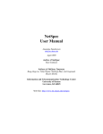
Packet transmission from the application starts in the process context. It continues in
the same context until the net device layer, where the packet gets queued. The network
device is checked to see if it is available for transmission. If the device is available, the
packet is transmitted in the process context, otherwise the packet is requeued and the
transmission is carried out in softirq context. Figure 3.2 gives the control flow through
the different layers when a packet is transmitted. The following section describes the
different steps in transmission.
23
Figure 3.2: Packet Transmission in the Linux Network Stack
24
Application Layer
Step 1:
The journey of a network packet starts from the application layer where a
user program may write to a socket using a system call. There many system calls that
can be used to write or send message from a socket. Some of these are send, sendto,
sendmsg, write and writev(). Here the execution of the system calls occur in the
process context.
Step 2:
It is worth mentioning that irrespective of the type of system call used, the
control finally ends up in the sock sendmsg [net/socket.c] function, which is used
for sending messages. This function checks if the user buffer space is readable, if so it
gets the sock structure using the file descriptor available from the user program. It
then creates a message header based on the message to be transmitted and a socket
control message containing information like the uid, pid and gid of the process. These
operations are also carried out in the process context.
Step 3:
The control then moves on to the layer implementing the socket interface.
This is normally the INET layer which maps the socket layer on to the underlying
transport layer. This INET layer extracts the socket pointer from the sock structure
and verifies if the sock structure is functional. It then verifies the lower layer protocol pointer and invokes the appropriate protocol. This function is carried out in the
inet sendmsg [net/ipv4/af inet.c] function.
Transport Layer (TCP/UDP)
Step 4 :
In the transport layer depending on the protocol being used, i.e., either TCP
or UDP the appropriate functions are invoked. These functions are also executed in
the process context.
In case of TCP, the control flows to the tcp sendmsg [net/ipv4/tcp.c] routine.
Here the socket buffer sk buff structure is created to store the messages to be transmitted. First the status of the TCP connection is checked and the control waits until
25
the connection is complete, if not completed previously. The previously created socket
buffer is checked to see if it has any tail space remaining to fit in the current data. If
available, the current data is appended to the previous socket buffer, otherwise a new
socket buffer is created to store the data. The data from the user space is copied to the
appropriate socket buffer and the checksum of the packet is calculated.
In case of UDP the control flows to the udp sendmsg [net/ipv4/udp.c] routine.
The routine checks the packet length, flags and the protocol used and builds the UDP
header. It verifies the status of the socket connection. If it is a connected socket, the
system sends the packet directly to the lower layer, else it does a route lookup based
on the IP address and then passes the packet to the lower layers.
Step 5 :
For a TCP packet the tcp transmit skb [net/ipv4/tcp output.c] rou-
tine is invoked which builds the TCP header and adds it to the socket buffer structure.
The checksum is counted and added to the header. Along with the ACK and SYN
bits, the status of the connection, the IP address and port numbers of the source and
destination machines are verified in the TCP header.
For a UDP packet, the udp getfrag[net/ipv4/udp.c] routine is invoked which
copies the data from the user space to the kernel space and calculates the checksum.
This function is called from the IP Layer, where the socket buffer for the packet is
initialized.
These functions are also executed in the process context.
Network Layer (IP)
Step 6 : The packet sent from the transport layer is received in the network layer
which is the IP layer. The IP layer receives the packet, builds the IP header for it and
calculates the checksum.
For a TCP connection, based on the destination IP address, it does a route lookup
to find out the output route the packet has to take. This is done in the user context in
the routine ip queue xmit [net/ipv4/ip output.c].
In case of a UDP connection, the IP layer creates a socket buffer structure to store
26
the packet. It then calls the udp getfrag() function mentioned above, to copy the
data from the user space to the kernel. Once this is done it directly goes to the link
layer without getting into the next step of fragmentation. These operations are done in
the ip build xmit [net/ipv4/ip output.c] routine.
Step 7 : In case of a TCP packet the ip queue xmit2 [net/ipv4/ip output.c]
routine checks to see if fragmentation is required in case the packet size is greater than
the permitted size. If fragmentation is needed, then the packets are fragmented and
sent to the link layer. This routine is executed in process context and is not required by
the UDP packets.
Link Layer
Step 8 :
From the link layer there is no difference in the nature of processing between
a TCP and a UDP packet. The link layer recieves the packet through the dev queue xmit [net/core/dev.c] routine. This completes the checksum calculation if it is not
already done in the above layers or if the output device supports a different type of
checksum calculation. It checks if the output device has a queue and enqueues the
packet in the output device. It also initiates the scheduler associated with the queuing
discipline to dequeue the packet and send it out. In this step the execution is carried
out in the process context.
Step 9 : The dev queue xmit routine invokes the qdisc run [include/net/pkt sched.h] routine which checks the device queue to see if there are any packets
to be sent out. If present, it initiates the sending of a packet. This function runs in the
process context the first time it comes through this flow of control, however if the device is not free or if the process is not able to send the packet out for some other reason,
this function is executed again in a softirq context.
Step 10 :
The qdisc run routine invokes the qdisc restart [net/sched/sch -
generic.c] function to check if the device is free to transmit. If so, the packet is sent
27
out to be transmitted through the driver specific routines.
Step 11 : In case the network device is not free to transmit the packet, the packet
is requeued again for processing at a further time. The scheduler calls the netif schedule [include/linux/netdevice.h] function which raises the NET TX SOFTIRQ, which would take care of the packet processing at the earliest available time.
Network Device Driver Layer
Step 12 :
The hard start xmit [drivers/net/device.c] function is an inter-
face to the device driver specific implementation used to prepare a packet for transmission and send it out.
Step 13 :
The device specific routines are then invoked to do the transmission. The
packet is sent out to the output medium by calling the I/O instructions to copy the
packet to the hardware and start the transmission. Once the packet is transmitted, it
also frees the socket buffer space occupied by the packet and records the time when
the transmission took place.
Step 14 :
Once the device finishes sending the packet out it raises an interrupt to
inform the system that it has finished sending the packet. If the socket buffer is not free
at this point in time, then it is freed. It then calls the netif wake queue [include/linux/netdevice.h], which is basically to inform the system that the device is free
for sending further packets. This function in turn invokes netif schedule to raise
the transmit softirq to schedule the transmission of the next packet.
3.5.3 Packet Reception in the Linux Network Stack
The control flow for receiving a packet from the network stack follows two flows of
execution. One from the user program in the application layer to the transport layer,
where the process blocks waiting to read from the queue of incoming packets. The execution in this flow is carried out in the process context. The other is the flow from the
28
arrival of a packet in the physical layer up to the transport layer, where the received
packets are put into the queue of the blocked process. This is carried out in a combination of hardirq and softirq contexts. Figure 3.3 gives the control flow of the different
steps in the reception of a packet which are discussed below.
Application Layer
Step 1 :
The user process reads data from a socket using the read or the variants of
the socket’s receive API calls like (recv and recvfrom). These functions are mapped
onto the sock read, sock readv, sys recvfrom and sys recvfrom system calls
which are defined in the net/socket.c file.
Step 2 : The system calls set up the message headers and call the sock recvmsg
[net/socket.c] function, which calls the receive function for the specific socket type.
In case of the INET socket type the inet recvmsg [net/ipv4/af inet.c] function
is called.
Step 3 : The inet recvmsg checks if the socket is accepting data and calls the corresponding protocol’s receiver function depending on the transport protocol used by
the socket. For TCP it is tcp recvmsg [net/ipv4/tcp.c] and for UDP it is udp recvmsg [net/ipv4/udp.c].
Transport Layer (TCP/UDP)
Step 4 : The TCP receive message routine checks for errors in the socket connection
and waits until there is at least one packet available in the socket queue. It cleans up
the socket if the connection is closed. It calls memcpy toiovec [net/core/iovec.c]
to copy the payload from the socket buffer into the user space.
Step 5 : The UDP receive message routine gets the UDP packet from the queue by
calling skb recv datagram [net/core/datagram.c]. It calls the skb copy datagram iovec routine to move the payload from the socket buffer into the user space.
29
Figure 3.3: Packet Reception in the Linux Network Stack
30
It also updates the socket timestamp, fills in the source information in the message
header and frees the packet memory.
This control flow from the application layer is blocked until data is available to
be read by the user process. The following section gives the flow of control from the
arrival of a packet in the network interface card up to the transport layer in the network
stack, where the user process is blocked waiting for data.
Step 6 : A packet arriving through the medium to the network interface card is checked
and stored in its memory. It then transfers the packet to the kernel memory using
DMA. The kernel maintains a receive ring-buffer rx ring which contains packet descriptors pointing to locations where the received packets can be stored. The network
interface card then interrupts the CPU to inform about the received packets. The CPU
stops its current operation and calls the core interrupt handler to handle the interrupt.
The interrupt handling occurs in two phases : hardirq and softirq. The hardirq
context performs the critical functions which need to be performed when an interrupt
occurs. The core interrupt handler invokes the hardirq handler of the network device
driver.
Net Device Layer
Step 7 :
This interrupt handling routine, which is device dependent, creates a socket
buffer structure to store the received data. The interrupt handler then calls the netif rx schedule [include/linux/netdevice.h] routine, which puts a reference to
the device in a queue attached to the interrupted CPU known as the poll list and
marks that further processing of the packet needs to be done as a softirq by calling
the cpu raise softirq [kernel/softirq.c] function to set the NET RX SOFTIRQ
flag. The control then returns from the interrupt handling routine in the Hardirq context.
In case of kernels which do not support NAPI [15] (for kernels before 2.4.20), the
interrupt handler calls the netif rx [net/core/dev.c] function which appends the
31
socket buffer structure to the backlog queue and marks that further processing of the
packet has to be done as a softirq by enabling the NET RX SOFTIRQ. If the backlog
queue is full the packet is dropped. For network drivers that do not make use of the
NAPI interface the backlog queue is still used by the 2.4.20 kernel for backward compatibility.
Step 8 :
When the NET RX SOFTIRQ is scheduled, it executes its registered handler
net rx action [net/core/dev.c]. Here the CPU polls the devices present in its
poll list to get all the received packets from their rx ring or from the backlog
queue, if present. Further interruptions are disabled until all the received packets
present in the rx ring are handled by the softirq. The process backlog [net/core/dev.c] function is assigned as the poll method of each CPU’s socket queue’s
backlog device. The backlog device is added to the poll list (if not already present)
whenever netif rx is called. This routine is called from within the net rx action
receive softirq routine, and in turn dequeues packets and passes them for further processing to netif receive skb [net/core/dev.c].
For kernel version prior to 2.4.20, net rx action polls all the packets in the backlog queue and calls the ip rcv procedure for each of the data packets. For other types
of packets (ARP, BOOTP, etc.), the corresponding ip xx routine is called.
Step 9 : The main network device receive routine is netif receive skb [net/core/dev.c] which is called from within NET RX SOFTIRQ softirq handler. It checks
the payload type, and calls any handler(s) registered for that type. For IP traffic, the
registered handler is ip rcv. This gets executed in Softirq context.
Network Layer (IP)
Step 10 :
The main IP receive routine is ip rcv [net/ipv4/ip input.c] which is
called from netif receive skb when an IP packet is received on an interface. This
function examines the packet for errors, removes padding and defragments the packet
32
if necessary. The packet then passes through a pre-routing netfilter hook and then
reaches ip rcv finish which obtains the route for the packet.
Step 11 :
If it is to be locally delivered then the packet is given to ip local deliver
[net/ipv4/ip input.c] function which in turn calls the ip local deliver finish
[net/ipv4/ip input.c] function to send the packet to the appropriate transport
layer function (tcp v4 rcv in case of TCP and udp rcv in case of UDP). If the packet
is not for local delivery then the routine to complete packet routing is invoked.
Transport Layer (TCP/UDP)
Step 12 :
The tcp v4 rcv [net/ipv4/tcp ipv4.c] function is called from the ip -
local deliver function in case the packet received is destined for a TCP process on
the same host. This function in turn calls other TCP related functions depending on
the TCP state of the connection. If the connection is established it calls the tcp rcv established [net/ipv4/tcp input.c] function which checks the connection status and handles the acknowledgements for the received packets. It in turn invokes
the tcp data queue [net/ipv4/tcp input.c] function which queues the packet
in the socket receive queue after validating if the packet is in sequence. This also updates the connection status and wakes the socket by calling the sock def readable
[net/core/sock.c] function. The tcp recvmsg copies the packet from the socket
receive queue to the user space.
Step 13 : The udp rcv [net/ipv4/udp.c] function is called from the ip local deliver routine, if the packet is destined to an UDP process in the same machine.
This function validates the received UDP packet by checking its header, trimming
the packet and verifying the checksum if required. It calls udp v4 lookup [net/ipv4/udp.c] to obtain the socket to which the packet is destined. If no socket is
present it sends an ICMP error message and stops, else it invokes the udp queue rcv skb [net/ipv4/udp.c] function which updates the UDP status and invokes
sock queue rcv skb [include/net/sock.h] to put the packet in the socket re33
ceive queue. It signals the process that data is available to be read by calling sock def readable [net/core/sock.c]. The udp recvmsg copies packet from the socket
queue to the user space.
3.6 NetSpec
NetSpec [9] [12] is a software tool developed by researchers at the University of Kansas
for the ACTS ATM Internetwork (AAI) project. It is used to automate the schedule of
experiments consisting of several machines over a distributed network.
NetSpec was originally intended to be a traffic generation tool for large-scale data
communication network tests with a variety of traffic source types and modes. It provides a simple block structured language for specifying experimental parameters and
support for controlling experiments containing an arbitrary number of connections
across a LAN or WAN.
Experiments to be carried out are specified as commands in a script file. One of
the nodes in the network acts as the NetSpec Controller which has the schedule of
experiments to be carried out. Daemon processes are initiated in the other nodes which
get the experiment schedule from the NetSpec Controller and perform the operations
specified in the script.
The single point of control and the ease of automating the experiments make NetSpec a valuable tool for conducting distributed experiments. It also supports transfer
of files both to and from the NetSpec controller machine. This feature is used to transfer configuration files for carrying out the experiment and for collecting the results at
the end of the experiment. The tests discussed in the Chapter 5 were carried out under
NetSpec control.
34
Chapter 4
Implementation
In order to transmit packets with a deterministic schedule it becomes necessary to identify the possible sources of delay within the kernel and to find out schemes to avoid
such delays during the transmission of a packet. One such scenario is in the handling
of the NET TX SOFTIRQ where the memory allocated for the packets that have completed transmission is freed before actually going on to process the transmission of the
next packet. Section 4.1 presents a scheme for removing this latency and its variance.
Section 3.5.2 discussed the control flow of the code performing packet transmission.
Its execution can occur in process context when the network device is free or can be set
to be carried out in the softirq context in case the network device is not available. In
order to control the packet transmissions it becomes necessary that we have the section
of code which handles packet transmissions to be executed only in the softirq context.
Section 4.2 discusses the modifications done to handle all packet transmissions in the
softirq context.
Controlling packet transmissions at specific instants of time requires scheduling
of the softirq, that handles packet transmission as and when it is required. This is
achieved by creating a new scheduling hierarchy using the Group Scheduling framework. Section 4.3 discusses the new Group Scheduling model required to support
Time Division Multiplexing and Section 4.4 describes about the scheduler required to
perform packet transmissions at specific instants of time.
Section 4.5 discusses the user level programs which are used to interact with the
35
kernel in creating the global transmission schedule and the command line utilities
available for controlling the TDM schedule.
4.1 Reducing Latency in Packet Transmission
In a Time Division Multiplexing scheme, each machine is provided with a specific time
slot for transmission. During the time slot, the machine must be involved only in
transmitting packets as much as possible. Any other non-critical operations are to be
delayed to a later time.
The handling routine for NET TX SOFTIRQ is net tx action [net/core/dev.c].
This routine is invoked whenever the NET TX SOFTIRQ is set and the do softirq
routine is invoked to service the pending softirqs. The net tx action routine goes
through the list of completion queues associated with the network devices, which contain socket buffers of packets that have been transmitted. The routine frees the memory
allocated for these socket buffers. Once this is done, the next packet to be transmitted is
dequeued from the queuing discipline associated with the network device, from which
the packet is to be transmitted. If the device is free, it invokes the transmitting routine
of the Ethernet driver to transmit the packet. In case the device is not available for
transmission, the packet is requeued and the NET TX SOFTIRQ is set to transmit the
packet next time this softirq is scheduled.
In this routine, clearly the initial step of freeing the memory allocated for transmitted packets can be delayed until a time, when it is not the time slot for transmission.
This will reduce the latency caused in packet transmission.
To achieve this, the handling routine of the NET TX SOFTIRQ is accordingly modified so as not to carry out this garbage collection process. Instead, we define a new
softirq called as NET KFREE SKB SOFTIRQ, which is used to free the socket buffers of
the transmitted packets. This is appended to the list of softirqs defined in the kernel.
(Softirqs are defined as an enumerated list in the include/linux/interrupt.h
file). Being the last softirq in the list, it is scheduled with the lowest priority, but functions effectively without affecting the packet transmission.
36
4.2 Packet Transmission in Softirq Context
In Section 3.5.2, we had seen the control flow in transmission of a packet through the
network stack in the kernel. The transmission of a packet starts from the application
layer where the process initiates sending of a packet. The packet transmission continues through the protcol stack until the network device layer, in process context, where
the packet gets enqueued in the Traffic Control layer queue.
Beyond this point, the execution can take place in either of the two contexts :
process context or softirq context. First the kernel starts to transmit the packet in
process context. In case the network device is not free to transmit the packet, the
NET TX SOFTIRQ is raised to handle the transmission. This carries out the transmission in softirq context. Figure 4.1 gives the control flow for the transmission of a packet
in the Vanilla Linux kernel.
Since we need to perform packet transmissions only at specified time instants, it
becomes necessary to control the computation that performs the transmission. Instead
of controlling the processes that need to transmit, modifications can be done in the
kernel so that packet transmissions are always carried out in softirq context from the
net device layer.
In order to achieve this, the control flow after enqueuing the packet is modified,
such that, the dev queue xmit routine invokes netif schedule through the send packet interface. The netif schedule routine enables NET TX SOFTIRQ, which is
then used to handle packet transmissions.
With the packet transmission being handled only by the softirq, the flexibility offered by the Group Scheduling framework to control the scheduling and execution of
softirqs can be used to have time triggered transmission of packets. Figure 4.2 gives
the modified control flow for packet transmission using TDM.
This modification can cause a slight delay in packet transmissions, as now the packets have to wait till the NET TX SOFTIRQ is scheduled for execution. However, the
ability to control the packet transmissions gained by this modification, offsets the small
delay incurred in its processing.
37
Figure 4.1: Network Packet Transmission in Vanilla Linux
38
Figure 4.2: Modified Network Packet Transmission for TDM
39
4.3 The TDM Model under Group Scheduling
The Group Scheduling model supported by KURT-Linux provides a generic framework which can be used to customise the way the interrupt servicing is handled. With
the flexibility to control the execution of hardirqs, softirqs, bottom-halves and processes, this framework allows the designer to specify a model with customised routines
for handling the execution of the different computational components.
Section 3.3.5 discussed the Vanilla Linux Softirq model which was used to mimic
the scheduling and execution semantics of softirqs in the Vanilla Linux kernel. This
section discusses the Group Scheduling model that would be required to support timetriggered transmission of packets implementing a Time Division Multiplexing scheme.
The scheduling hierarchy for the TDM model, shown in Figure 4.3, is comprised
of a Top group associated with a sequential scheduler. Under the Time Division Multiplexing scheme the transmission of packets is to be controlled based on time. For
this, the clocks on all the machines which are part of the TDM setup, need to be synchronized. This synchronization is achieved by using the modifications done to the
Network Time Protocol [17]. In order to maintain the time synchronization between
the machines and achieve a global schedule for transmission, it is necessary that time
related updates provided to each machine is reflected immediately by the machine’s
clock. The updates to the system time are carried out in the timer bottom half. Normally the timer bottom half is executed as a softirq by setting the HI SOFTIRQ bit. As
the accuracy of following a schedule within a machine is a prerequisite for handling
time triggered transmissions, we first need to have the timer bottom half executed before scheduling the transmit softirq. For this purpose, we have the timer bottom-half
added as the first member of the Top group.
As packet transmissions need to occur at specific instants of time, it is clear that the
transmit softirq NET TX SOFTIRQ must be provided with a higher priority for execution. For this purpose we define a new group called as the ’Transmit group’ and add it
as the second member of the Top group. This group is associated with a special TDM
scheduler. The NET TX SOFTIRQ is added to this Transmit group and is invoked based
on the decision made by the TDM scheduler.
40
Next, we need to process the remaining softirqs. For this, we create a new group
called as ’Softirq group’ which is associated with a sequential scheduler. The softirqs
defined in the kernel are added in order of their priority. So, the HI SOFTIRQ , NET TX SOFTIRQ, NET RX SOFTIRQ and the TASKLET SOFTIRQ are added in sequence. In
addition, the softirq which we created to free the socket buffers, namely NET KFREE SKB SOFTIRQ, is added as the fifth softirq in this group.
We have the NET TX SOFTIRQ present in two groups in this scheduling hierarchy.
When TDM is enabled, the packet transmission is carried out by the NET TX SOFTIRQ
member present in the Transmit group. When TDM is disabled, the transmission is
handled by the NET TX SOFTIRQ member present in the Softirq group.
Figure 4.3: TDM Model Scheduling Hierarchy
A global state variable named tdm status is used to maintain the status of the
TDM schedule in the kernel. Initially, when the kernel is booted, the tdm status
41
is initialised to TDM DISABLED. When the TDM schedule is submitted to the TDM
scheduler, the status is changed to TDM SCHEDULE SET. This reflects a state wherein a
TDM schedule is provided, but the TDM has not yet started on the machine. Once the
timer denoting the beginning of the transmission time-slot expires for the first time,
the TDM status is changed to TDM ENABLED.
4.4 The Time Division Multiplexing Scheduler
The Transmit group in the TDM model hierarchy is associated with a TDM scheduler, which is used to select the instants of time when the NET TX SOFTIRQ has to be
scheduled for transmitting the packets. In order to schedule packet transmissions at
periodic intervals in time, the kernel has to know the transmission start time, stop time
and interval period. Section 4.5 discusses how these values are provided to the kernel
from the user space. Once the start time is provided to the TDM scheduler, it creates a
UTIME kernel timer which is made to expire at the specified time. The UTIME timer
is made to operate in a privileged mode by setting the UTIME PRIV flag. This ensures
that the timer bottom-half is executed in the hardirq context.
The set transmit bit routine is the handling function when the timer expiration is used to denote the start of the transmission slot. When this routine is invoked for
the first timer expiration, it checks if the value of tdm status is TDM SET SCHEDULE,
if so it sets the state to TDM ENABLED, denoting the start of the TDM schedule. Then
this routine sets a local flag variable called as time to transmit to TRUE, which
allows the scheduler to schedule the softirq for transmission. The routine also sets
another kernel timer to expire when the transmission slot is supposed to end. The
reset transmit bit routine is used as the handler function for these timers denoting the end of a transmission slot. Program 4.1 gives the pseudo-code for the
set transmit bit handling routine.
The reset transmit bit routine as the name implies sets the time to transmit flag to FALSE, denoting the end of the transmission slot. This routine then calculates the expiration values for the beginning and the end of the time slots for the
42
Program 4.1 Pseudo-Code for the Timer handling routine invoked at the start of a
transmission slot
1 void set_transmit_bit(data)
2 {
3
if(tdm_status == TDM_SCHEDULE_SET){
4
tdm_status = TDM_ENABLED;
5
}
6
time_to_transmit = TRUE;
7
kernel_timer.expiration_jiffy = end_time_jiffies;
8
kernel_timer.expiration_subjiffy = end_time_subjiffies;
9
kernel_timer.handling_function = reset_transmit_bit;
10
set_kernel_timer(kernel_timer);
11 }
next transmission cycle. This is done by simply adding the transmission cycle jiffy
values to the current time-slot’s begin and end time values. It then sets up the kernel
timer to expire at the start time of the next interval. Now the set transmit bit routine is set as the timer handling routine. Program 4.2 gives the pseudo-code for the
reset transmit bit handling routine.
The TDM scheduler follows a simple policy of sequentially selecting its members
for execution. In this model the NET TX SOFTIRQ is the only member belonging to the
Transmit group. When the TDM Scheduler is invoked by the Top Group’s scheduler, it
selects the NET TX SOFTIRQ and performs the following checks. First, it checks if TDM
is enabled. If so, it checks if it is the time-slot for transmission. If that also happens to
be true, it verifies if there are any packets to be transmitted by checking the NET TX SOFTIRQ bit in the pending softirq flag field. Only when this condition evaluates to
true, does the TDM scheduler return the NET TX SOFTIRQ member to be scheduled. If
the either of these conditions fail, the scheduler returns a global pass member, denoting
that it doesn’t have any member to be scheduled. Program 4.3 gives the pseudo code
for the Scheduling Decision Function associated with the TDM scheduler.
43
Program 4.2 Pseudo-Code for the Timer handling routine invoked at the end of a transmission slot
1 void reset_transmit_bit(data)
2 {
3
time_to_transmit = FALSE;
4
5
begin_time_jiffies += period_jiffies;
6
begin_time_subjiffies += period_subjiffies;
7
while (begin_time_subjiffies >= subjiffies_per_jiffy) {
8
begin_time_jiffies++;
9
begin_time_subjiffies -= subjiffies_per_jiffy;
10
}
11
12
end_time_jiffies += period_jiffies;
13
end_time_subjiffies += period_subjiffies;
14
while (end_time_subjiffies >= subjiffies_per_jiffy) {
15
end_time_jiffies++;
16
end_time_subjiffies -= subjiffies_per_jiffy;
17
}
18
19
kernel_timer.expires = begin_time_jiffies;
20
kernel_timer.subexpires = begin_time_subjiffies;
21
kernel_timer.function = set_transmit_bit;
22
set_kernel_timer(kernel_timer);
23 }
Program 4.3 Pseudo-Code for the TDM Scheduling Decision Function
1 group_member tdm_scheduler (previous_task_struct, this_cpu,
2
group_member)
3 {
4
group_member = get_member_from_member_list();
5
if(group_member == NET_TX_SOFTIRQ){
6
if(tdm_status == TDM_ENABLED){
7
if(time_to_transmit == TRUE){
8
if(net_tx_softirq_is_pending){
9
return group_member;
10
}
11
}
12
}
13
}
14
return global_pass_member;
15 }
44
4.5 User Interface
A pseudo-device driver based approach is provided for the user space programs to
interact with the kernel. Section 4.5.1 presents the TDM controller pseudo device and
its associated driver, used for passing TDM schedule parameters to the kernel space.
Section 4.5.2 discusses the master-slave configuration for setting up the global TDM
schedule. The functionality of the TDM Slave Daemon and the TDM Master process are
discussed in Sections 4.5.3 and 4.5.4 respectively. The operations involved in starting
and stopping TDM are discussed in Sections 4.5.5 and 4.5.6.
4.5.1 The /dev/tdm controller Device
A pseudo device called /dev/tdm controller is created to provide interactions
with the kernel. A device driver built as a loadable kernel module interfaces this device with the user program. The device driver defines a set of I/O controls to the
tdm controller device. The I/O controls include options to submit a TDM schedule to the kernel and to stop the schedule. Special data structures are defined to pass
the parameters from the user space to the kernel.
4.5.2 TDM Master-Slave configuration
The network setup in which TDM is configured, is comprised of a TDM Master machine, which is used to form the global schedule and pass each slave machine its schedule for transmission. The slave machines in the network use this schedule provided
by the master for transmitting packets. One of the major hurdles in forming the global
schedule is that the number of machines that are going to be a part of the setup must be
known before-hand so that the transmission times for each machine can be determined.
This issue of determining the machine count can be achieved by either hardwiring a set
of machines to act as a part of the network or by using a configuration file to store the
list of machines that are to be a part of the TDM setup. These schemes have drawbacks
with addition and removal of machines from the TDM network. The selected approach
is to dynamically determine the number of machines before TDM schedule is formed.
45
This is achieved by having an initial handshake between the daemon processes in the
slave machines and the master program. The following sections describe in detail the
operation of the TDM Slave Daemon and the TDM Master process.
4.5.3 The TDM Slave Daemon
The TDM slave daemon process, tdmd, is started in the machines that are part of the
TDM Ethernet. The daemon process opens a socket connection and listens for a request
from the TDM Master. The machine which is acting as the TDM Master is provided
with the values regarding the TDM start time and the total transmission cycle, which
includes the transmission time-slots of all the machines in the setup.
The time-slot available for each machine in the Ethernet depends upon the number
of machines present in the network. Hence, before deciding upon the time-slot, it is
necessary that the TDM Master machine is aware of this number. In order to do this an
initial handshake is used between the TDM Master and the slave machines.
The daemon program sets up a UDP socket on a predefined port number listening
for the initial request from the TDM Master. Once it receives the first handshake from
the master, it responds back by sending its hostname. Once this is done, the UDP
socket is closed and a TCP socket is opened on a predefined port by the daemon. This
TCP connection then waits until it receives the schedule for that machine from the
TDM Master. The schedule is presented to the slave machines as a set of propertyvalue pairs which are then written into a configuration file, called tdm config. Once
this file is created, the daemon process uses the values present in the file to start the
TDM schedule. It invokes the ioctl call of the tdm controller device to submit the
schedule to the kernel.
4.5.4 The TDM Master
The TDM Master program is initiated in a machine which is to act as the master machine that forms the global TDM schedule. Any machine can be configured to act as
the TDM Master. The syntax for starting the TDM Master process is as follows :
46
tdm master <broadcast address> <minutes> <seconds> <total transmission cycle> where
<broadcast address> is the broadcast address of the LAN segment where
TDM is to be configured
<minutes> is the time in minutes from now when TDM is to be started
<seconds> is the time in seconds from now when TDM is to be started
<total transmission cycle> is the time in nanoseconds which includes
the transmission time-slots of all machines in the TDM network.
The first requirement of the master process is to determine the number of slave machines that are going to be a part of this TDM setup. This is achieved as a part of the
initial handshake between the master and the slave machines. The Master program
starts by creating a UDP socket and sends out a broadcast message to all the machines
in the network. The broadcast address used is the one specified in the command line,
when starting the TDM Master. The master then waits for a reply from the other machines in the network to respond to the broadcast message. Each of the machine that
has the TDM daemon running will reply to this broadcast message with their respective hostname. A reply period of 5 seconds is assumed for the client machines to reply
back. The replies received during that period decides the set of machines that will be a
part of the TDM setup.
Once the number of machines is determined, the master program forms the TDM
schedule. The total transmission cycle specified on the command line is used to calculate the individual time-slots available for each machine to transmit. Ideally the
time-slot size for each machine can be obtained by dividing the total transmission cycle by the total number of machines in the TDM setup. But in reality we need to take
into account the precision offered by the time synchronisation scheme in calculating
the transmission period within the time-slot. With unsynchronised clocks the transmission time-slots of two machines can overlap, which may result in collisions due to
the simultaneous transmissions. In order to avoid this we would need to provide some
47
safety separation between the transmission time-slots of the machines. This inter-timeslot gap can be defined as the ’buffer period’. The size of the gap will approximately
be twice the precision offered by the time synchronisation scheme employed. Section
5.2 discusses about the identification of an appropriate buffer period. When forming
the schedule, half of the buffer period value is removed from the start and end of a
transmission time-slot. This will provide disjoint intervals of transmission for each of
the machines in the network.
Each machine is provided information about when TDM is to be started in the
network, along with the expiration times for the start and end of the transmission slot
in that machine. This information is conveyed to the machines by means of a set of
property-value pairs defined as follows :
TDM START SEC - Wall clock time in seconds when the TDM schedule must start.
TDM START NSEC - Wall clock time in nanoseconds when the TDM schedule
must start.
TDM BEGIN SEC - Time in seconds when the time slot for transmission must start
relative to the start of cycle.
TDM BEGIN NSEC - Time in nanoseconds when the time slot for transmission
must start relative to the start of cycle.
TDM END SEC - Time in seconds when the time slot for transmission must stop
relative to the start of cycle.
TDM END NSEC - Time in nanoseconds when the time slot for transmission must
stop relative to start of cycle.
TDM PERIOD SEC - Total time period in seconds for each transmission cycle.
TDM PERIOD NSEC - Total time period in nanoseconds for each transmission cycle.
In order to obtain the actual start time values for TDM START SEC and TDM START NSEC, the master process first uses the gettimeofday system call to obtain the cur48
rent time in seconds and nanoseconds. The minute and second value provided in
the command line for starting the TDM Master are converted in order of seconds and
nanoseconds and added to the values obtained from the gettimeofday call. These
values denote when TDM is to be started in the network.
Depending upon the ordinality of the replies of the initial handshake received from
the slave machines, the time-slot’s begin and end times can be calculated. For this, first
the ideal time-slot size
is obtained by dividing the total transmission cycle
by the number of machines .
(4.1)
Taking into account the buffer period the effective time-slot size
"!$#&%'
for
transmission is given by
(' "!$#)%""*,+-
/.102
(4.2)
So for a machine with ordinality ’3 ’, where 3
+
begin time would be 340657.98
(:
;
varies between 1 and , the time-slot
. Half of the buffer period mentioned earlier
is included both in the beginning and the end of a time-slot. This correction is applied
to obtain the actual time-slot begin time
(<=?>A@
and end time
@B
for a machine of
ordinality 3 as follows :
<=?>C@D,+"+
( @J,+
3K8
3E0F57.B8
G
-"
(
.L0
.(H
+ = I
.
+ = I
.
(4.3)
(4.4)
Next the value for the time period after which the global transmission schedule repeats
is to be given to the machines. This will be the value of the total transmission cycle
specified in the command line when invoking the TDM Master process.
The master process ends after sending the schedule to all the machines. The slave
process on receiving the property-value pairs from the master, writes it to a configuration file called as tdm config.
49
4.5.5 Starting the TDM schedule
When the kernel is loaded with the TDM module, initially the TDM status, denoted
by the global variable tdm status is set to TDM DISABLED. Once the schedule is obtained by the daemon process it invokes an ioctl call through the device driver to submit the schedule to the TDM model in the kernel. The kernel timer which is to be
programmed needs to be provided with the expiration values for the beginning and
end of the time-slot. The TDM model validates the start time specified and submits
the expiration values and the transmission cycle period to the TDM scheduler, which
handles setting the timers. Once the schedule is submitted to the TDM scheduler, the
TDM status is changed to TDM SCHEDULED SET. This is an intermediate state denoting
that the schedule is provided and that TDM will be started depending on the start time
value specified in the command line.
Inside the TDM scheduler, the expiration times obtained in terms of seconds and
nanoseconds are converted into jiffies and subjiffies. Then the scheduler sets up a
UTIME kernel timer with the expiration values provided. On the expiration of this
timer the set transmit bit handling routine is invoked which sets the TDM status
to TDM ENABLED and thereby starts packet transmission using TDM.
4.5.6 Stopping the TDM schedule
The tdm user level program can be used to stop the TDM schedule using the stop
option. The syntax is as follows:
tdm stop
This is used to stop the TDM schedule in a particular machine. This option uses
the ioctl of the device driver to inform the kernel that TDM needs to be stopped. On
receiving this message the TDM model sets the TDM status to TDM DISABLED and
informs the TDM scheduler which removes the kernel timer.
50
Chapter 5
Evaluation
This chapter discusses the tests performed to evaluate our claim that, with Time Division Multiplexing it is possible to support real-time networking on Ethernet. The tests
carried out here are used to demonstrate that, by using Time Division as a scheme to
control access to the transmission medium, it is possible to make Ethernet deterministic
and achieve collision free packet transmission.
In order to employ TDM, it is required to select a transmission time slot for each
machine in the network. To do this, first we need to know the time taken to transmit
packets from a machine. Section 5.1 discusses the tests carried out to determine the
time taken for packet transmissions and its dependency on the packet size. The precision offered by the synchronising mechanism must also be taken into account while
forming the TDM schedule for each machine. Section 5.2 discusses the selection of
a suitable buffer period between two successive transmissions. The results obtained
from the above two sections are used in forming the TDM schedule for a set of machines in the network. Section 5.3 describes the steps in synchronizing the machines
and setting up the TDM Ethernet. The schedules formed are tested to show that collision free transmission is supported by TDM. Section 5.4 discusses these tests, for TDM
schedules of 3 different packet sizes. Finally, Section 5.5 presents a summary of the
results obtained. DSKI events and histograms where used to collect the data for the
tests and NetSpec was used to carry out the distributed tests.
51
5.1 Determining Packet Transmission Time
In order to decide upon the time-slot for transmission, we first need to determine the
time taken for transmitting a packet from a machine to another in an Ethernet. This
transmission time largely depends on the size
, of the packet being transmitted and
the link capacity , provided by the transmission medium. It is also affected by the
length of the physical link, which connects the two machines and the speed of light
in that medium. Theoretically the total time taken for packet transmissions,
#?#;
,
based on the above factors can be calculated as follows :
L#?#; ((!@%# (<G#$$:# >"@
H
: >
#@L9'
(5.1)
where
!@1%#L<G#$ L# >"@9 - (5.2)
and
L > ?#@: G' (5.3)
In most cases the distance between machines in a LAN is about a few meters and
hence the propagation delay is on the order of tens of nanoseconds, which is negligible
in this context. Thus the major factor determining the time for transmission is the time
taken to convert the message bits to signals in the physical medium.
For Ethernet, common link capacities are 10Mbps and 100 Mbps. The size of an
Ethernet frame can vary between 64 to 1518 bytes. The minimum size of an Ethernet
frame is 64 bytes including the Ethernet header and trailer of 18 bytes. Thus the minimum data payload supported by the Ethernet frame is 46 bytes. Payloads of smaller
size are padded up to get this minimum value. Of the 46 bytes, 20 bytes is taken by the
IPv4 header. Depending on the transport protocol used, TCP header takes a minimum
of 20 bytes and UDP takes 8 bytes. The remaining is the size of the actual data. The
52
maximum data payload size for the Ethernet frame is 1500 bytes.
For the experiment, we consider packet transmissions from a UDP based application. The minimum data size for a UDP application will be 46 - 20(IPv4 header) 8 (UDP header) = 18 bytes. Similarly the maximum data size will be 1500 - 20 - 8 =
1472 bytes. Table 5.1 gives the theoretical transmission times for an UDP application
of varying data sizes over 10Mbps and 100Mbps Ethernet.
Size of Data
(in bytes)
upto 18
64
128
256
512
1024
1472
Total Packet Size
(in bytes)
64
110
174
302
558
1070
1518
10Mbps Ethernet
(in s)
51.2
88
139.2
241.6
446.4
856
1214.4
100Mbps Ethernet
(in s)
5.12
8.8
13.92
24.16
44.64
85.6
121.44
Table 5.1: Theoretical Transmission times for 10Mbps and 100Mbps Ethernet
The experiment setup consisted of two 500MHz machines running the KURT-Linux
kernel, without any modifications to the network stack. The machines were connected
through a hub. In order to determine the transmission time, DSKI instrumentation
was used to collect histograms, measuring the time difference between two successive
reception of packets in the destination machine. A stream of about 400,000 packets
from an UDP application was transmitted from the source machine to the destination
machine. The experiment was carried out for both 10Mbps and 100Mbps Ethernet
with varying message sizes. The average transmission times measured for the varying
message sizes are presented as histograms.
Figures 5.1, 5.3 and 5.5 display the histograms for the packet transmission times
in a 10Mbps Ethernet. Figures 5.2, 5.4 and 5.6 display the histograms for the packet
transmission times in a 100Mbps Ethernet.
From the results shown in Table 5.2, it can be seen that the observed average transmission times for packets in a 10Mbps Ethernet are in agreement with the theoretical
values. In case of the 100 Mbps Ethernet, it can be seen that the average transmission
53
Packet_Transmission_Histogram_for_64_bytes_of_data_over_10_Mbps
Packet_Transmission_Histogram_for_64_bytes_of_data_over_100_Mbps
1e+06
1e+06
Min Value=82.9,Max Val=1971773.5;Underflow=0,Overflow=1
Total number of values : 414961
Min Value=74.6,Max Val=1333177.6;Underflow=0,Overflow=50
Total number of values : 414912
100000
No of values in each bucket <log scale>
No of values in each bucket <log scale>
100000
10000
1000
100
10
10000
1000
100
10
1
1
0
40
80
120
160
200
240
280
Bucket ranges in us (in us on a 497 Mhz machine)
320
360
399.987
0
Figure 5.1: Transmission time for packets
with 64 bytes of data in 10Mbps Ethernet
40
80
320
360
399.987
Figure 5.2: Transmission time for packets
with 64 bytes of data in 100Mbps Ethernet
Packet_Transmission_Histogram_for_256_bytes_of_data_over_10_Mbps
Packet_Transmission_Histogram_for_256_bytes_of_data_over_100_Mbps
1e+06
1e+06
Min Value=71.0,Max Val=142955.1;Underflow=0,Overflow=1
Total number of values : 414964
Min Value=57.8,Max Val=4145858.9;Underflow=0,Overflow=48
Total number of values : 414914
100000
No of values in each bucket <log scale>
100000
No of values in each bucket <log scale>
120
160
200
240
280
Bucket ranges in us (in us on a 497 Mhz machine)
10000
1000
100
10
10000
1000
100
10
1
1
0
50
100
150
200
250
300
350
Bucket ranges in us (in us on a 497 Mhz machine)
400
450
499.999
0
Figure 5.3: Transmission time for packets
with 256 bytes of data in 10Mbps Ethernet
54
40
80
120
160
200
240
280
Bucket ranges in us (in us on a 497 Mhz machine)
320
360
399.987
Figure 5.4: Transmission time for packets
with 256 bytes of data in 100Mbps Ethernet
Size of Data
(in bytes)
upto 18
64
128
256
512
1024
1472
Total Packet Size
(in bytes)
64
110
174
302
558
1070
1518
10Mbps Ethernet
(in s)
100.05
100.49
140.11
274.95
450.03
850.04
1275.14
100Mbps Ethernet
(in s)
95.17
94.94
96.31
96.01
98.87
99.64
122.51
Table 5.2: Observed Average Transmission times for 10Mbps and 100Mbps Ethernet
time is almost same for the smaller sized packets and increases for larger sizes. It can
be inferred that there is a minimum threshold limit on the time required for processing
a packet, which is independent of its size. This causes a more noticeable effect in case
of 100Mbps Ethernet than the 10Mbps. This is because the variation in transmission
times due to the packet size in case of 10Mbps Ethernet is more than the variation in
case of 100Mbps. So the fixed processing times influence the transmission times in case
of 100Mbps Ethernet, while the variable time to transfer bits into the media based on
the message size influences the transmission times in case of 10Mbps.
5.2 Time interval between successive packet transmissions
In order to have a global schedule with each machine transferring at a given point of
time, it is necessary that the machines in the network be synchronized with respect
to a common Time reference. Without synchronization, the transmission interval of
machines may overlap, resulting in collisions. The time synchronization scheme presented in [17] is used to achieve sychronization between machines in the Ethernet.
The precision offered by this clock synchronisation scheme is used to determine the
time interval between two consecutive transmissions so that the transmission timeslots of the machines do not overlap. The clock synchronisation scheme provides a
synchronisation of about 5 s difference from the global time for an average case and
about 16
s in the worst case. With a precision of +/- 5
55
s it is possible that two
Packet_Transmission_Histogram_for_1472_bytes_of_data_over_10_Mbps
Packet_Transmission_Histogram_for_1472_bytes_of_data_over_100_Mbps
1e+06
1e+06
Min Value=-3364563.3,Max Val=1670.6;Underflow=25,Overflow=0
Total number of values : 414960
Min Value=-1727457.7,Max Val=1438961.4;Underflow=1,Overflow=10
Total number of values : 414954
100000
No of values in each bucket <log scale>
No of values in each bucket <log scale>
100000
10000
1000
100
10
1000
100
10
1
500
10000
1
650
800
950
1100
1250
1400
1550
Bucket ranges in us (in us on a 497 Mhz machine)
1700
1850
2000
0
Figure 5.5: Transmission time for packets
with 1472 bytes of data in 10Mbps Ethernet
40
80
120
160
200
240
280
Bucket ranges in us (in us on a 497 Mhz machine)
320
360
Figure 5.6: Transmission time for packets
with 1472 bytes of data in 100Mbps Ethernet
machines can be apart by 10 s. So for an average case, the buffer period between two
consecutive time-slots must be atleast 10 s and in the worst case it may have to be as
high as 32 s. Following a cautious approach we settle on a value of 40 s for the buffer
period.
Figure 5.7 gives the formation of the global schedule for transmissions with the time
slots for transmissions of individual machines separated by the 40 s buffer period.
5.3 Setting up the TDM based Ethernet
The first step in setting up a TDM based Ethernet is to synchronize the clocks in the
machines forming the LAN. The time synchronization scheme presented in [17] is used
achieve synchronization between the machines. This is done in two steps : clock calibration and then clock synchronization. Each machine which is to be a part of the
TDM based Ethernet, is first calibrated to determine its clock tick rate. Then, one of the
machines in the network is configured as the Time Server. All other machines in the
network are synchronized with respect to this machine. The modified NTP daemon
56
399.987
Figure 5.7: Global TDM Transmission Schedule with Buffer Period
is started in the Time Server and time synchronisation daemons are run in the other
machines in the network. Synchronization updates are sent every 5 minutes to keep
the machines synchronized.
Once the time synchronisation is achieved, the user programs discussed in Section
4.5 are used to set up the TDM schedule. The tdmd daemon is initiated in all the
slave machines and the tdm utility is used to create the global schedule in the TDM
Master machine. The TDM Master sends each slave its transmission schedule. The
TDM schedule to be formed depends upon the number of machines in the Ethernet,
the transmission time for each machine and the buffer period discussed in Section 5.2.
Figure 5.8 gives our TDM setup composed of four 500MHz machines(A-D) connected by a 10Mbps Hub. Machine D was configured to act as the Time Server and
also as the TDM Master in this network. However, it is to be noted that any machine in
the Ethernet can act as the TDM Master. Based on the measured average transmission
times from Section 5.1, the time-slot for transmitting packets with a payload of 1500
bytes was chosen to be 1300 s. The TDM schedule hence formed consisted of 4 such
time slots separated by a 40 s buffer period.
The above setup was tested as follows. Two of the slave machines acted as Data
sources and third one as a Data sink. The parameters influencing the system are the
57
Figure 5.8: Ethernet with TDM
transmission queue length and the Maximum Transfer Unit (MTU) size of the network
interface. The transmission queue length was set to one to allow only one packet to be
transferred during a time slot. The MTU was left unaltered at 1500 bytes. The number
of collisions in each network interface is the metric to be measured. This is obtained
by using the ifconfig utility. A stream of 10,000 packets was generated from TCP
applications in both the Source machines to the Sink. This being a TCP application the
Sink machine transmits acknowledgement packets to both the Sources during its time
slot. Figure 5.9 gives the setup for this test.
After the test the network interfaces were found to have recorded no collisions
during the testing period. DSKI was used to collect packet reception events in the Sink
machine. The Tag field in the DSKI events was used to record the port number of the
packets received. From the DSKI events recorded on the Sink machine it was observed
that the Source machines transmitted packets alternatively in accordance with their
time slots. From the above experiment it was observed that with TDM it was possible
to achieve collision free transmissions on Ethernet.
58
Figure 5.9: Experiment setup with two sources and a sink
Based on the framework provided by [17] it was possible to collect events on different machines in the LAN and merge these based on a global timeline. DSKI instrumentation was used to collect the events denoting the start and end of the transmission
time slots in each of the machines in the TDM setup. The Datastreams postprocessing
was employed to merge these events on a global timeline and obtain intervals between
these events.
Figure 5.10 gives a screenshot of the transmission intervals for the three machines in
the TDM based Ethernet obtained from the Datastreams postprocessing visualization
having a time-slot of 220 s and a buffer period of 40 s. The lines above the interval
regions denote the start and stop events for the corresponding time-slot.
5.4 TDM schedules for varying packet sizes
As the transmission time varies with respect to the packet sizes it is possible to setup
TDM schedules suitable to the nature of the packet size being transmitted in the net59
Figure 5.10: Visualization of Transmission slots in TDM Ethernet
work. In this section we setup and evaluate TDM schedules for packets with payload
sizes of 64, 256 and 1500 bytes. The average transmission times give us a good starting
point in forming these time-slots. Our goal is to find time-slots suitable for transmitting
packets of the above mentioned sizes.
The first two sections determined the average time for transmission of a packet and
the buffer period to be used to take into account the precision offered by the time synchronisation scheme. Now based on these values we have the necessary information
to set up a TDM schedule and test its functionality.
The setup involves four 500MHz machines connected by 100Mbps hub, configured
to support TDM on Ethernet as described above. The parameters that affect the system
performance here include the transmission queue length and the MTU of the network
device. The transmission queue length is set to 1 so that only one packet is transmitted
during a given time-slot and the MTU size is set to a value which includes the sum
of the IP header, UDP header and the payload sizes. Multiple UDP applications of
varying load are run simultaneously to generate about a million packets. The test was
automated and run under NetSpec control. The number of collisions would indicate
how suitable the TDM schedule was to support transmission at high loads for a specific
packet size. Figure 5.11 gives the experiment setup.
60
Figure 5.11: Collision Test Experiment setup
61
The tests were repeated with varying timeslots until collision free transmission was
achieved. The following table lists the suitable time-slot values for transmission of
UDP packets of the given sizes.
Size of Data
(in bytes)
64
256
1472
Total Packet Size
(in bytes)
110
302
1518
Time slot in 100Mbps Ethernet
(in s)
220
260
440
Table 5.3: Transmission time-slots for 100Mbps Ethernet
5.5 Summary
We have shown that by employing Time Division Multiplexing scheme it is possible
to achieve determinism in Ethernet by having collision free transmisssions. We have
studied the transmission times for packets of various sizes for both 10Mbps and 100
Mbps Ethernet and have determined suitable time-slots for transmission for the different packet sizes in 100 Mbps Ethernet.
We have been able to achieve this with minimal modifciations to the existing KURTLinux code. Unlike [10], no modifications were done to the network stack to support
real-time applications. Time Division is an effective scheme for achieving contention
free access to the transmission media. The requirement to maintain time synchronization among the machines has often been the drawback for this scheme. However,
with the modified NTP Daemon [17] we have been able to achieve synchronization
within few tenths of microseconds which is suitable to support Time Division. Also
the modifications done are entirely in software and will be suitable to be used in any
Commercial-of-the-shelf Ethernet hardware.
Switches have replaced hubs offering double the bandwidth with no collisions. But
they do have issues of transmission latency due to the queuing in the output ports and
packet loss under high load. Our modifications can be applied for switched Ethernet
in order to avoid the queuing latency and packet loss.
62
Chapter 6
Conclusions and Future Work
Traditional Ethernet with its inevitable collisions and exponential backoff is not capable of supporting real-time applications present in industrial automation. Currently
available methods are not able to support the Quality of Service requirements of such
applications without employing special hardware and software. The requirement is to
provide a deterministic framework which can used to support the Quality of Service
requirements of the real-time applications on Ethernet.
The solution presented here is to employ Time Division Multiplexing on Ethernet.
With each machine in the LAN being given a disjoint time interval for transmission,
the possiblity of collisions is avoided. With no collisions, the random delay in packet
transmission due to the exponential backoff is also avoided and packet transmission
becomes deterministic. This provides a suitable framework for supporting real-time
applications over the Ethernet.
The solution is achieved entirely in software, with minimal changes to the existing
KURT-Linux kernel. There are no modifications to the network or transmission protocols, so the existing programs will continue to work as such. Both the real-time and
non real-time applications are supported by the same network stack, unlike [10] where
separate network stacks were required to support the two. This being a software solution, can be applied to any common Ethernet hardware and is suitable for real-time
applications used in industrial automation.
The modifications done here will provide deterministic access to the medium for
63
each of the machines in the network. With this deterministic access, it is possible to
develope Quality of Service schemes to be provided for the real-time applications.
With Linux 2.6 kernel, the timer bottom half handling is done as a Softirq. This
would require modifications to the existing Group Scheduling model for TDM in which
it is handled as a Bottom Half. In this case the modified Group Scheduling hierarchy
would consist of the TIMER SOFTIRQ as the first member instead of the TIMER BH.
Currently the schedules formed provide each machine in the network the same
fixed time for transmission. It is possible to construct a TDM schedule server which
would take into account many other constraints and form the schedule based on that.
For example, a machine which has larger volume of data to be transferred can be provided a longer time-slot for transmission. Thus the schedule formed will depend on
the QoS requirements for each of the machines in the network.
64
Bibliography
[1] Linux Cross Reference. http://lxr.linux.no/source.
[2] Network Time Protocol. http://www.ntp.org.
[3] Werner Almesberger. Linux Network Traffic Control - Implementation
Overview. Technical report, EPFL ICA, April 1999.
[4] Daniel P. Bovet and Marco Cesati. Understanding the Linux Kernel. O’Reilly, 2002.
[5] B. Buchanan, D. Niehaus, G. Dhandapani, R. Menon, S. Sheth, Y. Wijata, and
S. House. The Datastream Kernel Interface (Revision A). Technical Report
ITTC-FY98-TR-11510-04, Information and Telecommunication Technology
Center, University of Kansas, 1994 June.
[6] Curtiss-Wright Controls Embedded Computing. SCRAMNet+ Shared Memory
Speed, Determinism, Reliability, and Flexibility for Distributed Real-Time
Systems. http://www.systran.com/ftp/literature/sc/scsmwp.pdf.
[7] Will Dinkel, Douglas Niehaus, Michael Frisbie, and Jacob Woltersdorf.
KURT-Linux User Manual, 2002.
[8] Michael Frisbie. A Unified Scheduling Model Framework. Master’s thesis,
University of Kansas, March 2004.
[9] R. Jonkman. NetSpec: Philosophy, Design and Implementation. Master’s thesis,
University of Kansas, February 1998.
[10] Jan Kiska. RTnet - Hard Real-Time protocol for RTAI/Linux.
www.rts.uni-hannover.de/rtnet/index.html.
65
[11] Seok-Kyu Kweon, Min gyu Cho, and Kang G. Shin. Soft Real-Time
Communication over Ethernet with Adaptive Traffic Smoothing. In IEEE
Transactions on Parallel and Distributed Systems, October 2004.
[12] Radhakrishnan R. Mukkai. Design of the new and improved Netspec Controller.
Master’s thesis, University of Kansas, December 2003.
[13] Paulo Pedreiras, Lus Almeida, and Paolo Gai. The FTT-Ethernet Protocol:
Merging Flexibility, Timeliness and Efficiency. In 14th Euromicro Conference on
Real-Time Systems, 2002.
[14] Miguel Rio, Mathieu Goutelle, Tom Kelly, Richard Hughes-Jones, Jean Philippe
Martin-Flatin, and Yee-Ting Li. A Map of the Networking code in Linux Kernel
2.4.20, DataTAG-2004-1. Technical report, DataTAG, March 2004.
[15] Jamal Hadi Salim, Robert Olsson, and Alexey Kuznetsov. Beyond Softnet. In
Proceedings of the 5th Annual Linux Showcase and Conference, November 2001.
[16] Chia Shen and Ichiro Mizunuma. RT-CRM: Real-Time Channel-based Reflective
Memory. In 3rd IEEE Real-Time Technology and Applications Symposium, June 1997.
[17] Hariharan Subramanian. Systems Performance Evaluation Methods for
Distributed Systems Using Datastreams. Master’s thesis, University of Kansas,
2004.
[18] Andrew S. Tanenbaum. Computer Networks 3rd Edition. Prentice Hall, 1996.
[19] Chitra Venkatramani and Tzi cker Chiueh. Supporting Real-Time Traffic on
Ethernet. In Proceedings of IEEE Real-Time Traffic Systems Symposium, December
1994.
[20] Matthew Wilcox. I’ll Do It Later : Softirqs, Tasklets, Bottom Halves, Task
Queues, Work Queues and Timers. Linux.conf.au, 2003.
66