Download IN-PARALLEL PASSIVE COMPLIANT COUPLER FOR ROBOT

IN-PARALLEL PASSIVE COMPLIANT COUPLER FOR ROBOT FORCE CONTROL
By
CHAD M. TYLER
A THESIS PRESENTED TO THE GRADUATE SCHOOL
OF THE UNIVERSITY OF FLORIDA IN PARTIAL FULFILLMENT
OF THE REQUIREMENTS FOR THE DEGREE OF
MASTER OF SCIENCE
UNIVERSITY OF FLORIDA
2000
ACKNOWLEDGMENTS
The author greatly acknowledges the support of the Center for Intelligent
Machines and Robotics at the University of Florida for providing a Research
Assistantship, as well as the facility and equipment to carry out this work. The
Department of Energy is also gratefully acknowledged for its support via grant through
the University Research Program in Robotics.
ii
TABLE OF CONTENTS
page
ACKNOWLEDGMENTS .................................................................................................. ii
LIST OF TABLES ............................................................................................................. iv
LIST OF FIGURES..............................................................................................................v
ABSTRACT....................................................................................................................... vi
INTRODUCTION................................................................................................................1
SYSTEM PERFORMANCE SPECIFICATIONS AND DESIGN .....................................5
Platform and Robot Performance Tasks .............................................................................5
Design of the Platform ........................................................................................................8
Kinematic Model of the Platform .....................................................................................17
Software Algorithm ..........................................................................................................18
EXPERIMENTAL RESULTS...........................................................................................21
Potentiometer Calibration ..................................................................................................21
Force/Torque Measurements..............................................................................................22
Joystick Application...........................................................................................................24
CONCLUSIONS/FUTURE WORK..................................................................................25
APPENDIX A COMPUTER CODE .................................................................................27
APPENDIX B PCCFC PART DRAWINGS .....................................................................59
LIST OF REFERENCES ...................................................................................................88
BIOGRAPHICAL SKETCH .............................................................................................89
iii
LIST OF TABLES
Table
1
2
3
4
page
Steel Sheet Dimensions..............................................................................................14
Desired Load and Compliance Characteristics. .........................................................17
Potentiometer Calibration Values. .............................................................................20
Wrench Comparison Data..........................................................................................21
iv
LIST OF FIGURES
Figure
1
2
3
4
5
6
7
8
9
page
Passive In-Parallel Platform on a Serial Robot. ..........................................................2
System Loop. ..............................................................................................................6
In-Parallel Mechanism. ...............................................................................................8
Top view of 3-3 Parallel mechanism structure. ........................................................10
Compliant Platform Simulation Software. ................................................................12
Section of Captive Ball Joint with Teflon Plates. .....................................................13
Connector Springs. ....................................................................................................14
Leg Assembly/ RRRP Mechanism. ...........................................................................16
PCCFC Computer Rendering. ..................................................................................26
v
Abstract of Thesis Presented to the Graduate School
of the University of Florida in Partial Fulfillment of the
Requirements for the Degree of Master of Science
ROBOT FORCE CONTROL USING AN IN-PARALLEL PASSIVE COMPLIANT
COUPLER
By
CHAD M. TYLER
AUGUST 2000
Chairman: Dr. Carl D. Crane III
Major Department: Mechanical Engineering
This thesis presents the design of a Passive Compliant Coupler for Force Control
(PCCFC) as well as the method for controlling the contact force and orientation of a robot
manipulator with the coupler. To accomplish these tasks, a compliant parallel platform
was designed and built and then connected through both physical hardware and computer
software to a Puma industrial robot. The platform consists of six connectors that are
linearly compliant structures of known spring rate with a mechanism in each that allows
its change in length to be measured.
A forward displacement analysis is performed using the connector length values.
This analysis provides the position and orientation of the top platform with respect to the
base. Line coordinates can be computed for each connector from these values. The
wrench being applied to the platform is then computed using the their line coordinates
and connector lengths. This wrench is then used to modify the robot end effector position
vi
and orientation in order to get a force and orientation combination acceptable to the
particular task being performed.
vii
CHAPTER 1
INTRODUCTION
The use of an in-parallel passive compliant force-torque sensor can improve the
capabilities of a serial manipulator by allowing for the control of position and contact
force. This is done by taking readings from the force-torque sensor in the form of analog
voltage data from six rotary potentiometers. The data is then transformed into the lengths
of the six platform connectors. The data is then used to compute the pose of the top plate
of the platform with respect to the bottom plate and then to modify the path for the serial
robot to follow. The goal of this modification is to allow the serial robot manipulator to
maintain a desired force and contact orientation with objects in the workspace.
In order to get six degrees of control, the force-torque sensor must have the
geometry such that we can compute the twist it is experiencing as a result of the serial
robot movement. Further, to control the torque being generated through the sensor by the
serial robot, the stiffness properties of the sensor device must be known. With the twist
and stiffness known, the wrench being applied to the sensor can be computed [Griffis and
Duffy 1991]. The desire to have six degrees of freedom leads to the use of an in-parallel
mechanism.
The in-parallel mechanism has a high load bearing capacity and the geometric
properties of load distribution. This is due to the fact that the connectors sustain the load
in a parallel fashion. Further, the geometry of the parallel mechanism allows for a
compact design. For these reasons, the parallel mechanism is a good candidate to use in a
1
2
serial manner with a serial robot without changing the workspace of the serial robot or the
robot's normal operating procedures. The small size will allow the parallel mechanism to
be attached as the end effector of the robot arm and the lightweight nature of the
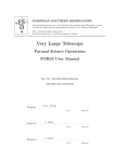
mechanism will not adversely affect the robot arm performance. A drawing of a passive
in-parallel platform connected at the end of a serial robot is shown in figure 1.
Fig 1. Passive In-Parallel Platform on a Serial Robot
There are advantages to using a passive compliant structure to control force and
displacement simultaneously as opposed to active compliant force control methods.
When the lengths of the connectors of the parallel platform are adjusted using servos, a
linear relationship between the force and displacement can be computed [Sugar and
Kumar 1998]. This active method does not allow for the simultaneous control of both
force and displacement. There are other methods to control forces by controlling
positions or controlling positions and forces together, such as compliant control,
3
compliance and force control and hybrid control. These methods require more
complicated means of control than the passive compliance control.
On the other hand passive compliance motion control can accommodate the
misalignments that exist between the robot manipulator and the object it is manipulating
due to geometrical uncertainties and manufacturing tolerance of the parts. Passive
compliance is therefore qualified to sustain the required contact force between two
interacting surfaces and most importantly would assist in the smooth transition of forces
from the no contact mode region to contact with the environment. The simple and realtime response of passive control avoids the complex controller and sophisticated
instrumentation required in some industrial applications. The in-parallel mechanism
offers a straightforward and easy method to reconstruct the wrench applied on one of the
plates from calculated connector forces, therefore the Passive Compliant Coupler for
Force Control (PCCFC) can provide force feedback control of the robot. It is different
from commercially available Remote Center Compliance (RCC) devices that are open
loop systems and not meant to sense the applied wrench and hence cannot provide force
feedback control of the robot.
Gaillet and Reboulet [1983] developed the first sensor of this kind based on the
octahedral structure of the Stewart platform. Nguyen et al [1991] reported the
development of a Stewart platform based sensor with LVDT’s mounted along the legs for
wrench measurement in the presence of a passive compliance. Bhaumick et al [1997]
reported the development of a stiff force-torque sensor based on the Stewart Platform
with shape optimization of the legs to minimize the Noise to Signal ratio. Various
authors carried out theoretical investigations of the behavior of the Stewart platform
4
sensor. Svinin and Uchiyama [1995] have considered the optimality of the condition
number of the force transformation matrix. The optimum condition number criterion has
to be exercised with utmost care. Though the optimum configuration appears to present
an isotropic solution, the neighborhood solutions (configurations) may deteriorate very
fast and could be close to singularity. Therefore the condition number criteria can be at
best limited to stiff Stewart Platform Sensors [Dasgupta, et al 1994, Bhaumick et al 1997]
where change in structural configurations is not anticipated and the condition number
remains the same. Lee et al [1996] defined the problem of ‘closeness’to a singularity
measure by defining what is known as Quality Index (QI) for planer in-parallel devices.
Lee et al [1998] extended the definition of Quality Index to spatial 3-3 in-parallel devices.
The quality index is the ratio of the absolute value of the determinant of the Jacobean of
the platform in some arbitrary position to the maximum absolute value of the determinant
that is possible for the same in-parallel mechanism. However there is no proper
mathematical basis to compare the performance of the two in-parallel systems as yet. The
practical implementation of the parallel device based on theoretical studies present
numerous problems. Hunt and McAree [1998] present an in-depth implication of such
constraints and realistic design ideas.
CHAPTER 2
SYSTEM PERFORMANCE SPECIFICATIONS AND DESIGN
Platform and Robot Performance Tasks
The goal of this project was to develop a system that uses real-time data from the
PCCFC to modify the movements of a PUMA700 industrial robot. This was done using
5V potentiometers as the output devices from the PCCFC that send their data to an ADC
card that was installed in an IBM-PC running MS-DOS. The PC is also connected via
two serial ports to the PUMA700. One of these ports allows the PC to take over control
of the robot terminal program used to initialize the robot and transmit commands back
and forth. The other terminal is attached to the robots "alter" port. This port's function is
to allow the PC to send path modification data to the robot in real time. The PC is also
used to run the software necessary to receive the real-time data from the PCCFC,
transform it to usable connector length values, and then perform a forward analysis of the
PCCFC in order to obtain the wrench that is acting on the PCCFC. This wrench is then
used to calculate a modification to the robot end effector pose, which is then transmitted
via the serial connection to the PUMA700. The data being transmitted contains six
numerical values which represent the x, y and z translations and the rotations about those
three axis of the top plate with respect to the bottom plate. Therefore, a loop is created
starting from the PCCFC on to the PC then to the PUMA700 and finally back to the
PCCFC, as shown in figure 2.
5
6
Fig 2. System Loop
The objective of this thesis was to design a small passive compliant coupler based
on an in-parallel mechanism for force control. The desired load supporting ranges and
compliance characteristics are given in Table 1. The resolution of the platform in
measuring forces and torques are also listed in the table. The values shown in the table
are with respect to a right handed co-ordinate system (xyz) defined at the center of the
bottom plate, such that z is parallel to Z and x passes through a point O (see fig. 3).
Table 1: Desired Load and Compliance Characteristics
Sensing Axis
Ranges
Compliance
Resolution
Fx
±25 N
±4 mm
0.25 N
Fy
±25 N
±4 mm
0.25 N
Fz
±60 N
±8 mm
0.25 N
Mx
±500 N-mm
18 0
2.5 N-mm
My
±500 N-mm
18 0
2.5 N-mm
Mz
±1000 N-mm
18 0
2.5 N-mm
7
The desired size of the platform was less than four inches tall and a base diameter
of about six inches, so that it would be a good size to fit onto the end of the PUMA700
robot arm. The actual platform is only 3.5 inches tall and has a base diameter of 6.75
inches. The platform had to be light enough to not greatly impact the performance of the
PUMA700, which can support a 50 pound load during normal operation. The final
platform weight was between one and two pounds. More importantly than the actual
values for the load supporting and compliance characteristics of the platform is that the
platform can actually improve the capabilities of the PUMA700, which will be shown in
chapter 3 of this thesis.
Several experiments were done prior to getting to the point of controlling the
robot in real time with the PCCFC mounted on the PUMA700 end effector. The first of
these experiments was a sampling of the potentiometer outputs. The data was collected
with the platform under zero load conditions several times to get a range of values. The
values were then used to calibrate the individual potentiometers and eventually set the
zero value for each potentiometer in the control program.
The second experiment was a wrench calibration of the PCCFC using weights of
known mass. The weights were place on the top plate of the PCCFC and then data was
taken using the PCCFC software. The wrench generated in the platform was then
compared to the theoretical values for the force and torques that the weights would apply
over the given geometry. This allowed the platform to be calibrated for output of the
wrench data.
The third experiment was very similar to the final system, the difference being
that the PCCFC was mounted to a table rather than the PUMA700 end effector. With the
8
PCCFC mounted to a table, a wrench was applied to the top platform. The computer
software then took that wrench and applied an opposite scaled twist to the robot end
effector. The result is a sort of "joystick" application that allows the user to move the
robot end effector anywhere in the workspace. The next step would be to mount the
PCCFC on the PUMA700 and develop some tasks for the robot to perform using it's new
capabilities.
Design of the Platform
The six-degree of freedom in-parallel mechanism has six connectors, they are
connected through spherical joint balls in a pair wise manner at the top and at the base.
The top and bottom surfaces are planar for the sake of simplicity. The in-parallel
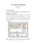
mechanism in its best form should be fully triangulated to form a 3-3 octahedron. A
schematic sketch of the in-parallel mechanism is given in figure 3. This simple kinematic
structure is complex to design. One, because of the problem of designing concentric
R
S
T
X
Q
P
Z
Y
Fig 3. 3-3 In-Parallel Mechanism
joint balls and the other is due to the mechanical interference of closely arranged legs.
9
Concentric ball joints could have been used in this application, however they
would have required a large amount of development and design time to produce. The
problems of using concentric joint balls were overcome by separating the center of the
joint balls by a small distance as to avoid possible interference problems. The overall
size of the platform was adjusted as needed to avoid connector to connector and
connector to platform interferences.
To overcome the interference of connectors, various ways of locating a leg along
intended line coordinates were considered. One way was to separate the balls by moving
them an equal distance away from and towards the center of the platform. A second way
was to keep one ball joint at the optimal location and moving the other ball joint either
towards or away from the center of the platform. In this case, the joint ball pairs were
separated by locating one at the optimal position at each corner of the top and bottom
platform and then moving the other joint balls in a counter-clockwise fashion along the
sides of the triangles that connect the optimal positions. The legs were connected from
the outside to inside and inside to outside positions going from the bottom to the top
platform. The distance between the centers of each pair of ball joints was dependent on
maintaining enough clearance between ball joints once the entire platform was built so
that the legs could have a range of motion suitable to the platforms intended workspace.
The distance between the ball joints was not the only factor to consider to configure the
platform for optimum range of motion. The actual size of the bottom and top platform
triangles had to be decided along with the separation or height of the top plate with
respect to the bottom plate.
10
The kinematic structure and the relative dimensions of the platform mechanism
were obtained by applying the optimal Quality Index criteria [Lee, et. al, 1998]. The
Quality index (QI) is defined by the following dimensionless expression
λ=
DetJ
(1)
DetJ m
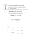
where, DetJ is the determinant of the Jacobean. The 6 by 6 matrix formed by the line coordinates of the 6 legs gives the Jacobean matrix of the mechanism. The normalized
determinant of the Jacobean, DetJ, at the central position and when both base and
platform are parallel (as shown in figure 4) is given by
a
b
Fig 4. Top view of 3 – 3 Parallel mechanism structure
3 3a 3b 3 h 3
(2)
3
 a 2 − ab + b 2

4
+ h2 


3


Where a and b are the sides of the equilateral triangle of the platform and the base
DetJ =
respectively, h is the height of the platform measured from center of the base plate to the
center of platform along z axis (see figure 3). The above expression is optimized to find
11
the expression for maximum |DetJ|. The maximum QI occurs when either of the
following two parametric relationships is satisfied.
b = 2 a;
h = a;
or
a = 2b;
h = b;
(3)
With these maximized values in mind, the platform was designed so the length of
a side of the bottom triangle is equal to twice that of the top triangle and the height at the
home(unloaded) position is equal to the length of a side of the top triangle. Given those
geometric ratios, there was still the matter of deciding what the size of the bottom triangle
would be and also what the separation distance of the ball joints would be. The approach
taken to solve this problem was a graphical one. A program was written using a
Microsoft Windows interface with OpenGL 3d graphics being displayed in that interface.
The program displays a 3d model of the platform which changes as data is altered
through various user input toggles and sliders on the interface. The program was setup so
that the user can change both the side length of the base triangle, which would in turn
change the top triangle and height dimensions, and the separation distance of the ball
joints. The program also allows the user to modify the pose of the top plate of the
platform by setting the value of the x, y and z translations and any combination of
rotations about any axis in the x-y plane that passes through the center of the top plate.
This important fact allows the user to see if the platform components will interfere with
each other inside of the platforms usable workspace. The parts of the platform that were
dimensionally fixed were the size of all the parts of each of the legs except for the lengths
of the parts that connect the spherical balls to the middle section of the legs. In this
manner, the overall lengths of the legs were also adjusted as changes were made to the
12
platform dimensions. There are numerical outputs on the program interface that display
the length of each leg that can be used for the final design length of each leg once the
other dimensions are satisfactorily selected. These leg lengths were also used to test the
forward analysis program, since this was a quick way to get six leg lengths for the
platform in different poses. The program allows the user to quickly adjust the important
Fig 5. Compliant Platform Simulation Software
dimensional parameters of the platform and to immediately get a visual display of what
the platform will look like in a wide range of poses(see Figure 5). The use of the program
led to the following dimensions of the platform:
b = 123.0 mm;
a = 61.5 mm;
ball joint separation distance = 14.0 mm;
long leg length = 83.0 mm;
short leg length = 77.7 mm;
13
Each of the six legs is a serial SPS (spherical-prismatic-spherical) chain. The leg
has a ball at either end that is held captive by a socket on the platform. The socket is a
captive arrangement of thin Teflon plates surrounded by aluminum plates, both with
counterbored holes in them that encapsulate each of the joint balls on two sharp edges
and allow for a large range of motion(figure 6). This construction was used to get a low
friction and predictable spherical joint.
Fig 6. Section of Captive Ball Joint with Teflon Plates
The mechanism in the middle of the leg consists of some thin sheets of spring
steel arranged in a serial and parallel way in order to get as much compliance as possible
in a small space, while maintaining enough lateral stiffness to prevent the leg from
buckling(figure 7(b)). The outer four sheets of steel are thinner than the two sheets in the
middle of the leg assembly. The spring constant of each connector was calculated by
assuming that each of the thin sheets of steel behaves as two cantilever beams(one beam
on either side of the middle parts of the leg assembly) in pure bending and then
calculating the force contained in each individual sheet given the maximum allowable
14
displacement and adding them together according to the serial/parallel way that they are
connected(figure 7(a)). Therefore, there are eight outer beams and four inner beams.
Fig 7. Connector Springs
7(a) Elastic elements of the leg
7(b) Compact arrangement of elastic elements
The steel sheets have the dimensions given in Table 1. These dimensions are then put
into the following equation for the deflection of a beam.
Fl3
δ=
3EI
(4)
bd 3
I=
12
(5)
E= 200000 MPa
(6)
The outer and inner springs are then combined into a total deflection of the connector.
δtotal = 8δinner + 4δouter
(7 )
δtotal = 0.0508F + 0.0241F
(8)
15
The variable F in equation 8 has units of Newtons and δ
total has units of millimeters. The
relationship between the spring constant of the outer and inner springs and the force and
deflection is known, so the overall spring constants were computed as
K connector =
(9)
2 K outer K inner
2 K outer + K inner
where,
K inner = 41.5 N / mm
K outer = 19.7 N / mm
Thus, the calculated overall spring constant for each connector was determined to be
Kconnector = 20.2N/mm. This value was used to compute the stiffness matrix for the
platform in order to do the wrench calculations.
Table 2: Steel Sheet Dimensions
Position
Height
Width
Bendable Length
Quantity
Outside
0.010"(0.254mm)
4 mm
11.0 mm
8
Inside
0.015"(0.381mm)
5 mm
11.0 mm
4
Attached to the body of the leg is a RRRP(R represents a revolute joint and P
represents a prismatic joint) planar mechanism where the spring section serves as a
compliant variable length link(figure 8). The motion of the 3-link mechanism is used to
rotate the shaft of a rotary potentiometer that is mounted into one of the pieces of the
middle section of the leg. The potentiometer has +/-5Vdc output, which can be used to
16
produce a range of values for the rotation that can be then be transformed into a change in
the overall length of the leg, utilizing the given geometry of the 3-link mechanism. The
compliance of the leg allows it to change length up to +/-4mm. This amount of length
change translates to +/-30o of rotation of the potentiometer shaft. The calculated change
in length can be added to the original length of the leg and therefore the platform will
produce six leg length values in real-time.
Fig 8. Leg Assembly/ RRRP Mechanism
The detailed design of the PCCFC was done in AutoDesk Mechanical Desktop.
Detailed part drawings of all of the parts needed to manufacture the platform are included
in Appendix-B. Also included at the beginning of Appendix-B is a list of all those
drawings and the quantities and material type of each part needed.
17
Kinematic Model of the Platform
r
To make a static force analysis, an external wrench W0 = [ Fx, Fy, Fz, Mx, My, Mz ]
(a force acting through the origin, together with a general couple M) is applied to the
movable platform. The external wrench is in static equilibrium with the six leg forces,
the equation representing this is given by
6
r
W0 = ∑ f i sˆi
(10)
i =1
where f i (i =1,..,6 ) are the magnitudes of the axial reaction forces experienced by the legs
and sˆi ( i =1,..,6) are the line co-ordinates of the legs. The system of forces remains in static
equilibrium as the moveable platform twists relative to ground. To account for the twist,
the external wrench changes as the platform moves. The mapping of the change in
wrench to the twist of the platform is given by
δWˆ = [ K ]δDˆ
(11)
r r
f ;δ
m0 ] is the change in wrench, which is mapped via 6 ×6 stiffness matrix
where δWˆ = [δ
[K] to the twist of the movable platform relative to the ground. The six twist co-ordinates
r r
give the twist δDˆ = [δx0 ; δφ] . The expression for the global stiffness is given by Griffis
and Duffy [1991] as
T
T
[K ]= []
j[
k i ][]
j + [
δjθ ][
k i (1 − ρ )][
δjθ ] + [
δjα ][
k i (1 −
T
T
+ [
δjθ ][
k i (1 − ρ )][
vθ ] + [
δjθ ][
k i (1 − ρ )][
vα ]
ρ )][
δjα ]
T
(12)
18
Where the columns of the 6 ×6 matrices [j], [
δjθ ]and [
δjα ]are line coordinates.
The i th column of [j] is the line co-ordinate for the line $ i for the i th leg, the i th column
δjθ ]is the line coordinate of the derivative δ$θi with respect to the appropriate θ .
of [
θi defines the elevation angle of the plane of the triangle, which is formed by the end
points of the i th connector with the adjacent connector that shares the base edge, from the
XY plane. ρi is the ratio of free length to the new length of the i th leg ( l 0i li ). The i th
δjα ]is the line coordinate of the derivative δ$αi with respect to the
column of [
appropriate α i . The α i defines the oriented angle of the i th connector measured from the
base edge. [
vθ ]and [
vα ]are 6 ×6 matrix moment vectors and are explained in Griffis and
Duffy [1991]. From equation 10, the wrench acting on the top platform can be calculated
from the six individual leg forces. Equations 11 and 12 can then be used to determine
what infinitesimal twist(of the top platform with respect to the base) is required in order
to achieve some infinitesimal change in the wrench applied to the top platform. A
simpler form of equation 3, which was used in the PCCFC software, is
δWˆ = J [ K ]δl
(13)
where J is the platform jacobian, K a 6X6 matrix with the spring constants of each
connector along the diagonal and δl is the change in length of each connector. This
equation is valid near the home position of the platform.
Software Algorithm
The software to perform the tasks outlined in the above section was written using
a Borland C compiler in an MS-DOS environment. For this example consider the case
19
where the in-parallel platform is attached to the end effector of the PUMA robot. Also
assume that the top of the platform is rigidly connected to ground. A user will specify a
desired wrench that is to be experienced by the top platform. The objective is to
determine how to move the PUMA end effector in order to realize this wrench. The flow
of the software is as follows:
1- Initialize the robot
2- Send starting message to the robot
3- Receive starting message reply from robot
4- Begin running in "absolute alter" mode
5- Obtain 6 potentiometer readings and transform them to 6 leg lengths
6- Reduce the special 6-6 geometry to the 3-3 geometry
7- Calculate the equivalent 3-3 leg lengths
8- Send the 3-3 leg lengths to the forward analysis program
9- Compute all real solutions for the platform pose
10- Select best pose solution according to which is closest to previous pose
11- Use the pose to calculate the twist and wrench of the top platform
12- Calculate the error wrench, i.e. the difference between the desired wrench and
the measure wrench
13- Determine the infinitesimal twist to move in order to reduce the error wrench
14- Scale the translation and rotation data according to the wrench
15- Send the transformation data to the robot through the alter port
Repeat starting at step 5
20
The process to calculate the stiffness matrix and wrench in the platform was
outlined in the preceding section. The geometric reduction was done using an algorithm
explained in Griffis[1993]. There were two corrections to the equations listed in this
Patent publication. Equation 33 on page 27 should read as,
(o0r1)2 = K0 + K1(o0o1)2 + K3(p0p1)2 + K4… … .
In Equations 35 on page 28, the 3rd and 4th equations should read as follows:
(p0t1)2 = k2 + m2(p0p1)2 - B(p0s1)2
(q0t1)2 = k5 + m5(t0t1)2 - E(p0t1)2
The computer code equivalent of the reduction equations are listed in the computer code
listing in Appendix-A, in the function "solve_georedux".
The forward analysis was done using the function "solve_platform", also listed in
the computer code listing in Appendix-A. The algorithm for this forward solution was
taken from Griffis and Duffy[1989].
CHAPTER 3
EXPERIMENTAL RESULTS
Potentiometer Calibration
The potentiometers were calibrated after final assembly of the platform. This was
done by taking 5000 samples from each potentiometer, while the platform was in its
home(unloaded) position, and writing them directly to a file. The readings were taken in
groups of 500 samples, 10 times for each potentiometer in order to get a wide range of
data. In between each data acquisition the top plate of the platform was moved/rotated
and then allowed to return to its home position. This was done to identify the dead zones
of the potentiometers. The maximum unassembled sample range of the potentiometers is
from 2048 to 4096 counts, corresponding to 300 degrees of rotation. In order to utilize
the full range of sampling capability of the potentiometers, the voltage sent to the
potentiometers had to be increased inversely proportional to the amount of the rotation
range being used. When the potentiometers are in the platform they can only rotate +/30o, which is one fifth of the total range. Therefore, the potentiometers were given 25V
of power to utilize their entire sample range. The averages of all the data taken are listed
in Table-3, along with their standard deviations.
The value of the standard deviation for each potentiometer was used to set up the
range of values considered to be zero for each potentiometer. This range was calculated
21
22
by setting any sample taken that was within the standard deviation to zero. The length of
the platform connectors can change 8mm overall. The change in length was divided by
the
Table 3: Potentiometer Calibration Values
Pot.
1
2
3
Average
Reading
91.9
Standard
Deviation
31.4
Measurement
Range
2048(+/-1024)
Percent of
Range(%)
1.5
Resolution
(mm/count)
0.0039
128.1
35.3
2048
1.7
0.0039
-116.4
34.0
2048
1.6
0.0039
4
5
54.9
50.5
2048
2.4
0.0039
-280.7
34.4
2048
1.7
0.0039
6
247.8
47.2
2048
2.3
0.0039
measurement range to get the resolution of each connector. The resolution of each
connectors is 0.0039mm/count. The main reasons for the large standard deviations of the
potentiometer data are: considerable amount of friction inside the potentiometer and
slipping between the potentiometer shaft and the RRRP mechanism. The difficulty of
which to get very accurate measurements from the potentiometers in this sort of platform
configuration is a definite reason to pursue use of other types of sensing devices in future
platform devices.
Force/Torque Measurements
In order to test out the platform software wrench calculations, weights were
placed on the top plate of the platform and readings were taken using the PCCFC
software. The weights were placed directly over the center of the top plate. The
coordinate system used to calculate the wrench has it's origin at one corner of the bottom
23
plate, refer to Figure 3. Therefore, a mass placed on the center of the top plate generates
force mainly in the direction of the Z-axis and torques over the X-Y plain. The wrench
data taken for several different loads is given in Table-4, along with theoretical values of
the forces and torques that would be generated by the given load and geometry.
Table 4: Wrench Measurement Data
Load
(lbs.)
14
10
5
Wrench
Component
Fx
Fy
Fz
Mx
My
Mz
Fx
Fy
Fz
Mx
My
Mz
Fx
Fy
Fz
Mx
My
Mz
PCCFC software
(lbs. and in.-lbs.)
0.114
-3.518
-15.984
-11.724
38.386
-12.542
-0.295
-0.318
-10.703
-13.539
25.404
-3.160
0.784
-0.638
-4.248
-3.950
12.16
-4.218
Theoretical
(lbs. and in.-lbs.)
0.0
0.0
-14.0
-19.6
33.9
0.0
0.0
0.0
-10.0
-14.0
24.2
0.0
0.0
0.0
-5.0
-7.0
12.1
0.0
Direct Error
0.114
3.518
1.984
7.88
4.486
12.542
0.295
0.318
0.703
0.461
1.204
3.16
0.784
0.638
0.752
3.05
0.06
4.218
The wrench measurement data shows a good correlation between the theoretical
force being placed in the Z-direction and the platforms wrench output of that force.
Forces along the X and Y-axis did not change much as expected under the vertical load.
The moments produced by the weights about the X and Y-axis corresponds closely to the
theoretical values. The worst part of the data is the large measurement discrepancies in
the data of the moment about the Z-axis as compared to the theoretical values.
24
Joystick Application
The software listed in Appendix-A was written to communicate with a PUMA700
industrial robot in real-time. The software controls the movement of the robot by sending
it values for the twist that is placed on the top plate of the PCCFC. The result of this is
the ability to move and orient the end effector of the robot in 6 degrees of freedom, in a
much faster and more natural way than previously possible using either a computer
terminal or the PUMA700 Teach Pendant. The compliant nature of the PCCFC coupled
with the ability to do a forward analysis using its connector lengths makes this application
possible.
CHAPTER 4
CONCLUSIONS/FUTURE WORK
This thesis has presented the design of an In-parallel passive compliant force
torque sensor and it's ability to be used to control an industrial robot. During the design
of the platform many of the important design issues associated with parallel platforms
have been addressed. There is the compact arrangement of elastic elements in the
platform connectors that allow a large compliance in a small space. The use of 3D
visualization during the design process was introduced to further assist in making the
platform as compact as possible. The need for a ball joint that had very low friction while
maintaining strength under dynamic loads led to the design of the captive Teflon ball
joints. Measuring the change in length of the connectors was accomplished using rotary
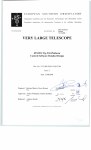
potentiometers and a 3-link mechanism. A computer rendering of the final design of the
PCCFC is presented in figure 9.
The ability of the platform to measure a wrench in a compliant manner is crucial
to the future use of such a device. The compliance will allow the platform to be used as a
compliant wrist element on a serial robot. This will allow the robot to encounter
obstacles in its workspace without immediately damaging those objects. The platforms
wrench output could be used to maintain a desired wrench on such an object. This can be
done by modifying the code in Appendix-A so that it uses the wrench calculations to
modify the twist data that is sent to the PUMA700 in a way that will maintain the desired
wrench. The code will also have to be altered to include instructions for the desired robot
25
26
task, currently the code only modifies the position of the robot from whatever position it
starts out at when the program is run. If the platform is used in this manner it will
improve the capabilities of the serial robot.
Fig 9. PCCFC Computer Rendering
In summary, the primary objective of designing and fabricating an in-parallel
platform that met the performance criteria listed in Table 2 was attained. This design is
documented in detail in Appendix B. In addition the methodology is presented as to how
the device could be used in the future as an attachment at the end of an industrial robot in
order to control contact forces. This implementation represents the significant work to be
accomplished in the future.
APPENDIX A
COMPUTER CODE
/*
Program: PCCFC Software
Programmers: Chad Tyler
Date: June 30, 2000
This program computes the geometric reduction
of the special 66 parallel platform to the 33
and then performs a forward analysis on the 33
platform leg lengths. The program then calculates
the wrench in the platform.
*/
#include
#include
#include
#include
#include
#include
#define
#define
#define
#define
#define
#define
#define
#define
#define
<stdio.h>
<conio.h>
<dos.h>
<stdlib.h>
<math.h>
<string.h>
BASE_ADC
CHAN
BASE_ALTER
BASE_TERM
CR 13
DEL 0xff
DLE 0x90
STX 0x82
ETX 0x83
0x220
6
0x3f8
0x2f8
/*
/*
/*
/*
/*
/*
base address of DT8214 ADC card
number of channels to convert
base address of ALTER serial port
base address of terminal serial port
carriage return
control characters ...
#define TRUE 1
#define FALSE 0
#ifndef D2R
#define D2R
#endif
0.01745329
#ifndef R2D
#define R2D 57.29577951
#endif
#define Sqrt(x)
#define Fabs(x)
sqrt((double)(x))
fabs((double)(x))
typedef struct Polyy{
int deg;
double coef[37];
double eval(double x);
} Poly ;
double Poly::eval(double x)
{
int i ;
27
*/
*/
*/
*/
*/
*/
28
double result = coef[0] ;
double val ;
if (deg > 0)
result += coef[1]*x ;
for (i=2 ; i<=deg ; i++)
{
val = pow (x, (double)i) ;
result += val * coef[i] ;
}
return (result) ;
}
void
void
void
void
pmult( Poly a, Poly b, Poly *c );
psub( Poly a, Poly b, Poly *c );
padd( Poly a, Poly b, Poly *c );
pscale( Poly a, double s, Poly *as );
void sample(int *, int);
/* ADC sampling function */
void setport(int address,int baud);
/* initialise serial port
int ALTER_recve(unsigned char *rx_msg,char initflag);
/* receive ALTER message
*/
void ALTER_tran(int *data_word,char initflag);
/* transmit ALTER message */
void rx(int address,int no,unsigned char *ch);
/* receive array over serial port */
void tx(int address,int no,unsigned char *ch);
/* transmit array over serial port*/
void transmit(unsigned char *string, int base, int count);
/* transmit to VAL terminal */
*/
void get_leglengths (double Ladc[6], int ad_value[6]);
void solve_georedux (double L_o0o1,double L_s0s1,double L_p0p1,double
L_t0t1, double L_q0q1,double L_r0r1,double Lsfor33[6]) ;
void solve_platform (int *pnum_solutions, double T_2_1[8][4][4],
double p_x_1, double q_x_1, double q_y_1,
double s_x_2, double t_x_2, double t_y_2,
double L_or, double L_os, double L_ps,
double L_pt, double L_qt, double L_qr) ;
int solve_bestsolution (int pnum_solutions, double r_1[8][4],
double s_1[8][4], double t_1[8][4], double movexyz[3]);
void matmult(double ans[4][4], double matrix1[4][4],
double matrix2[4][4]);
void matmult66(double bans[6][6],double bmatrix1[6][6],
double bmatrix2[6][6]);
void matvecmult6616(double cwrench[6], double cmat[6][6],
double ctwist[6]);
void vecmult(double ans1[4], double matrix1[4][4], double vector1[4]);
double dotproduct(double vector1[3], double vector2[3]);
void crossproduct(double ans[3], double vector1[3], double vector2[3]);
double vecmag(double vector[3]);
int valuenear (double x, double goal, double tol) ;
void Inverse(double matdata[], int numcol, double *det,
double invary[]);
void MatSwap(double *s1, double *s2);
void Transpose(double *a, double *b, int m, int n);
void findangles(double T_2_1[8][4][4], double newang[3], int bestanswer,
int rotx);
void findwrench(double jac[6][6], double jactp[6][6], double k[6][6],
29
double wrench[6], double movexyz[3],double newang[3]);
void wrench2(double jac[6][6],double Knew[6], double wrench[6]);
void setjac(double s[3][6], double jac[6][6]);
void main()
{
/* base points are o, p, and q
// 1st coordinate system origin is at o, p is
// on x axis, q is in xy plane
// upper platform points are r, s, and t
// 2nd coordinate system origin is at r, s is
// on x axis, t is in xy plane
// input items*/
double p_x_1, q_x_1, q_y_1 ;
double s_x_2, t_x_2, t_y_2 ;
double L_or, L_os, L_ps, L_pt, L_qt, L_qr, //virtual 33 leg lengths
L_oo, L_ss, L_pp, L_tt, L_qq, L_rr;//reassigned 66 leg lengths
double Ladc[6], Lsfor33[6];
//virtual 33 leg lengths
/* output items*/
double T_2_1[8][4][4];
int num_solutions ;
double movexyz[3], newang[3];
FILE *fpout;
fpout = fopen ("out6l.dat","w");
/******************************************************************/
/*
*/
/*
ALTER_9.C
- This program runs External ALTER in
*/
/*
absolute mode, using VAL program ALTERCUM, and makes use
*/
/*
of an external potentiometer connected to a DT8214 ADC
*/
/*
whose base address is set at 0x220. A single channel
*/
/*
is used to drive the selected axis of the robot
*/
/*
*/
/*
Set up to transmit with line ALTER(0,23) as follows:
*/
/*
The decimal mask value - ALTER input data enabled (16),
*/
/*
transmit matrix back to host (4), ALTER input data is in
*/
/*
World coordinates (2), ALTER input data is cumulative (1).
*/
/*
[See Table 3-1, Part 3 of VAL manual]
*/
/*
*/
/*
Uses COM1 (on PC) and the ALTER port (J123) on the VAL
*/
/*
controller, and uses an external ascii file (try X5.dat)
*/
/*
with path modification data to modify X & Y coordinates
*/
/*
to 'draw' a small circle in the X-Y plane.
*/
/*
*/
/*
Before running this program you must ensure that the robot
*/
/*
has been calibrated, the arm-power is on, and the arm is
*/
/*
at the #PSTART location - and away from any obstacles.
*/
/*
Use program TERMINAL.C to do this.
*/
/*
*/
/*
When ALTER is running hit any key to abort!
*/
/*
*/
/*
R.Bicker August 1999
*/
/******************************************************************/
unsigned char tran_char1[30],ch;
unsigned char rx_msg[19];
/* Bytes received from ALTER */
int ALTER_data[6] = {0,0,0,0,0,0}; /* 16-bit ALTER data
*/
int count=0;//,loopcount=0;
int ad_value[CHAN];
30
/* Initialize both serial ports */
setport(BASE_ALTER,0x3);
// baud rate set at 38400
setport(BASE_TERM,0x0c);
// baud rate set at 9600
strcpy(tran_char1,"ex altercum"); // Tranmit string via terminal
transmit(tran_char1, BASE_TERM ,11);// to execute ALTER program in
VAL
outportb(BASE_TERM ,CR);
delay(1);
// Send Carriage return!
printf("ALTER should now be running\n");
printf("check 0\n ");
if(ALTER_recve(rx_msg,1) == 1) exit(0); // Check initial ALTER
message,
delay(1);
printf("check 3 \n ");
// abort if error in received message
ALTER_tran(ALTER_data,1);
// Transmit initial PC
message.
delay(1);
while(!kbhit()) /* continuous loop - communication with ALTER */
{
//
count++;
//
printf("count = %5d \n",count);
sample(ad_value,CHAN);
get_leglengths(Ladc,ad_value);
L_oo
L_ss
L_pp
L_tt
L_qq
L_rr
=
=
=
=
=
=
Ladc[0];
Ladc[1];
Ladc[2];
Ladc[3];
Ladc[4];
Ladc[5];
solve_georedux(L_oo,L_ss,L_pp,L_tt,L_qq,L_rr,Lsfor33);
p_x_1 = 123.0 ;
/*location of p along x-axis*/
q_x_1 = 61.5 ;
/*location of q along x-axis*/
q_y_1 = 123.0*sin(60.0*D2R) ;/*location of q along y-axis*/
s_x_2 =
t_x_2 =
t_y_2 =
L_or
L_os
L_ps
L_pt
L_qt
L_qr
=
=
=
=
=
=
61.5 ;
/*location of s along x-axis*/
30.75 ;
/*location of t along x-axis*/
61.5*sin(60.0*D2R) ;/*location of t along y-axis*/
Lsfor33[0]
Lsfor33[5]
Lsfor33[4]
Lsfor33[3]
Lsfor33[2]
Lsfor33[1]
;
;
;/*33 leg lengths*/
;
;
;
solve_platform (&num_solutions, T_2_1, p_x_1, q_x_1, q_y_1,
s_x_2, t_x_2, t_y_2,
L_or, L_os, L_ps, L_pt, L_qt, L_qr) ;
int i, j, k, bestanswer ;
double r_1[8][4], s_1[8][4], t_1[8][4];
double vr2[4], vs2[4], vt2[4];
for(i=0; i<num_solutions ; ++i)
31
{
for(j=0; j<4 ; ++j)
{
r_1[i][j] = 0.0;
s_1[i][j] = 0.0;
t_1[i][j] = 0.0;
}
}
vr2[0] = 0.0 ;
vs2[0] = s_x_2 ;
vt2[0] = t_x_2 ;
vr2[1] = 0.0 ;
vr2[2] = 0.0 ; vr2[3] = 1.0 ;
vs2[1] = 0.0 ;
vs2[2] = 0.0 ; vs2[3] = 1.0 ;
vt2[1] = t_y_2 ; vt2[2] = 0.0 ; vt2[3] = 1.0 ;
for (i=0 ; i<num_solutions ;
{
for (j=0 ; j<4 ; ++j)
{
for (k=0 ; k<4 ; ++k)
{
r_1[i][j] +=
s_1[i][j] +=
t_1[i][j] +=
}
}
}
++i)
T_2_1[i][j][k]*vr2[k];
T_2_1[i][j][k]*vs2[k];
T_2_1[i][j][k]*vt2[k];
bestanswer = solve_bestsolution (num_solutions, r_1, s_1, t_1, movexyz);
int rotx;
if ((r_1[bestanswer][3]-t_1[bestanswer][3])<0.0)
rotx = 1;
else
rotx = -1;
findangles(T_2_1, newang, bestanswer, rotx);
double jac[6][6], Knew[6];
Knew[0]
Knew[1]
Knew[2]
Knew[3]
Knew[4]
Knew[5]
=
=
=
=
=
=
10.2*(Ladc[0]-83.0);
10.2*(Ladc[1]-77.7);
10.2*(Ladc[2]-83.0);
10.2*(Ladc[3]-77.7);
10.2*(Ladc[4]-83.0);
10.2*(Ladc[5]-77.7);
setjac(s, jac);
double wrench[6];
wrench2(jac, Knew, wrench);
fprintf(fpout,"%8.3f %8.3f %8.3f %8.3f %8.3f %8.3f \n",
wrench[0]*0.2248, wrench[1]*0.2248, wrench[2]*0.2248, wrench[3]*0.00885,
wrench[4]*0.00885, wrench[5]*0.00885);
printf("%7f %7f %7f %7f %7f %7f \n", wrench[0]*0.2248,
wrench[1]*0.2248, wrench[2]*0.2248, wrench[3]*0.00885,
wrench[4]*0.00885, wrench[5]*0.00885);
printf("check4 %d \n ", count);
if(ALTER_recve(rx_msg,0) == 1) //exit(0); // Abort if error in
received message
{
printf("Err check5 \n ");
32
exit(0); // Abort if error in received message
}
ALTER_tran(ALTER_data,0);
// Transmit ALTER data
// update ALTER_data[0] to ALTER_data[5] - 6-axis channel
data
ALTER_data[0]
ALTER_data[1]
ALTER_data[2]
ALTER_data[3]
ALTER_data[4]
ALTER_data[5]
=
=
=
=
=
=
-movexyz[0];
movexyz[1];
movexyz[2];
newang[0]*3;
newang[1]*3;
-newang[2]*3;
}
}
/*
Function to get the 6 leg lengths from the Analog-to-Digital
converter card.
*/
void get_leglengths (double Ladc[6], int ad_value[6])
{
Ladc[0] = 83.0
Ladc[1] = 77.7
Ladc[2] = 83.0
Ladc[3] = 77.7
lengths, 3072
Ladc[4] = 83.0
Ladc[5] = 77.7
+
+
+
+
(((ad_value[0]-3072)/10)-55.0)/25;
(((ad_value[1]-3072)/10)-7.0)/25;
(((ad_value[2]-3072)/10)+13.0)/25;
(((ad_value[3]-3072)/10)-3.0)/25;//set new leg
+ (((ad_value[4]-3072)/10)+28.0)/25;
+ (((ad_value[5]-3072)/10)-19.0)/25;
}
/*
Function to reduce the special 66 platform geometry to the
33 geometry in order to calculate the 33 leg lengths to send
to the "solve_platform" function to do a forward analysis
*/
void solve_georedux(double L_o0o1,double L_s0s1,double L_p0p1,
double L_t0t1,double L_q0q1,double L_r0r1,
double Lsfor33[6])
{
double o0p0, o0s0, p0q0, p0t0, q0o0, q0r0, s0p0, t0q0, r0o0,
r1s1, r1o1, s1t1, s1p1, t1r1, t1q1, o1s1, p1t1, q1r1,
A, B, C, D, E, F, k1, k2, k3, k4, k5, k6,
K0, K1, K2, K3, K4, K5, K6,
m1, m2, m3, m4, m5, m6;
o0p0
o0s0
p0q0
p0t0
q0o0
q0r0
s0p0
t0q0
r0o0
r1s1
r1o1
s1t1
s1p1
=
=
=
=
=
=
=
=
=
=
=
=
=
123;
109;
123;
109;
123;
109;
14;
14;
14;
61.5;
47.5;
61.5;
47.5;
33
t1r1
t1q1
o1s1
p1t1
q1r1
A
B
C
D
E
F
=
=
=
=
=
=
=
=
=
=
=
61.5;
47.5;
14;
14;
14;
o1s1/r1o1;
p1t1/s1p1;
q1r1/t1q1;
s0p0/o0s0;
t0q0/p0t0;
q0r0/r0o0;
k1
k2
k3
k4
k5
k6
=
=
=
=
=
=
(o1s1*r1o1)
(p1t1*s1p1)
(q1r1*t1q1)
(s0p0*o0s0)
(t0q0*p0t0)
(r0o0*q0r0)
m1
m2
m3
m4
m5
m6
=
=
=
=
=
=
r1s1/r1o1;
s1t1/s1p1;
t1r1/t1q1;
o0p0/o0s0;
p0q0/p0t0;
q0o0/r0o0;
+
+
+
+
+
+
(o1s1*o1s1);
(p1t1*p1t1);
(q1r1*q1r1);
(s0p0*s0p0);
(t0q0*t0q0);
(q0r0*q0r0);
K0 = (k6 - k3 + C*k5 - C*E*k2 + B*C*E*k4 - B*C*D*E*k1)/(F A*B*C*D*E);
K1 = (-B*C*D*E*m1)/(F - A*B*C*D*E);
K2 = (B*C*E*m4)/(F - A*B*C*D*E);
K3 = (-C*E*m2)/(F - A*B*C*D*E);
K4 = (C*m5)/(F - A*B*C*D*E);
K5 = (-m3)/(F - A*B*C*D*E);
K6 = (m6)/(F - A*B*C*D*E);
Lsfor33[0] = sqrt(fabs(K0 + K1*L_o0o1*L_o0o1 + K2*L_s0s1*L_s0s1 +
K3*L_p0p1*L_p0p1 + K4*L_t0t1*L_t0t1 +
K5*L_q0q1*L_q0q1 + K6*L_r0r1*L_r0r1));//or
Lsfor33[1] = sqrt(fabs(k1 + m1*L_o0o1*L_o0o1 A*Lsfor33[0]*Lsfor33[0]));//os
Lsfor33[2] = sqrt(fabs(k4 + m4*L_s0s1*L_s0s1 D*Lsfor33[1]*Lsfor33[1]));//ps
Lsfor33[3] = sqrt(fabs(k2 + m2*L_p0p1*L_p0p1 B*Lsfor33[2]*Lsfor33[2]));//pt
Lsfor33[4] = sqrt(fabs(k5 + m5*L_t0t1*L_t0t1 E*Lsfor33[3]*Lsfor33[3]));//qt
Lsfor33[5] = sqrt(fabs(k3 + m3*L_q0q1*L_q0q1 C*Lsfor33[4]*Lsfor33[4]));//qr
}
/*
Function to perform forward analysis of 33 stewart platform
*/
void solve_platform (int *pnum_solutions,
double T_2_1[8][4][4],
double p_x_1, double q_x_1, double q_y_1,
double s_x_2, double t_x_2, double t_y_2,
34
double L_or, double L_os, double L_ps,
double L_pt, double L_qt, double L_qr)
{
int poly_solve(double root_r[], double root_c[], int d, double
coeff[]) ;
int i ;
double
p_1[0]
p_1[1]
p_1[2]
q_1[0]
q_1[1]
q_1[2]
vk[0]
vk[1]
vk[2]
p_1[3], q_1[3], vk[3];
= p_x_1;
= 0.0;
= 0.0;
= q_x_1;
= q_y_1;
= 0.0;
= 0.0;
= 0.0;
= 1.0;
double L_op, L_pq, L_oq ;
L_op = vecmag(p_1);//sqrt(p_1[0]*p_1[0] + p_1[1]*p_1[1] +
p_1[2]*p_1[2]);//!p_1 ;
L_oq = vecmag(q_1);//sqrt(q_1[0]*q_1[0] + q_1[1]*q_1[1] +
q_1[2]*q_1[2]);//!q_1 ;
L_pq = sqrt(fabs((p_1[0] - q_1[0])*(p_1[0] - q_1[0])
+(p_1[1] - q_1[1])*(p_1[1] - q_1[1])
+(p_1[2] - q_1[2])*(p_1[2] - q_1[2])));//!(p_1 - q_1) ;
double
s_2[0]
s_2[1]
s_2[2]
t_2[0]
t_2[1]
t_2[2]
s_2[3], t_2[3];
= s_x_2;
= 0.0;
= 0.0;
= t_x_2;
= t_y_2;
= 0.0;
double L_rs, L_rt, L_st ;
L_rs = vecmag(s_2);//sqrt(s_2[0]*s_2[0] + s_2[1]*s_2[1] +
s_2[2]*s_2[2]);//!s_2 ;
L_rt = vecmag(t_2);//sqrt(t_2[0]*t_2[0] + t_2[1]*t_2[1] +
t_2[2]*t_2[2]);//!t_2 ;
L_st = sqrt(fabs((s_2[0] - t_2[0])*(s_2[0] - t_2[0])
+(s_2[1] - t_2[1])*(s_2[1] - t_2[1])
+(s_2[2] - t_2[2])*(s_2[2] - t_2[2])));//!(s_2 - t_2) ;
double
double
double
double
c41, s41, c34, s34, c12, s12, c23 ;
c41_o, s41_o ;
c41_p, s41_p ;
pxq[3];//cross product of p_1 and q_1
/* four bar at point O ////////////////////////////////////////*/
c41_o = c41 = dotproduct(p_1,q_1)/(L_op*L_oq);
crossproduct(pxq,p_1,q_1);
s41_o = s41 = (pxq[2]/(L_op*L_oq))*vk[2];
c23 = (L_or*L_or + L_os*L_os - L_rs*L_rs) / (2.0*L_or*L_os) ;
c34 = (L_os*L_os + L_op*L_op - L_ps*L_ps) / (2.0*L_os*L_op) ;
s34 = sin(acos(c34)) ;
35
c12 = (L_oq*L_oq + L_or*L_or - L_qr*L_qr) / (2.0*L_oq*L_or) ;
s12 = sin(acos(c12)) ;
/* First equation
AA1 y^2 x^2 + BB1 x^2 + CC1 y^2 + DD1 x y + EE1 = 0
double AA1, BB1, CC1, DD1, EE1 ;
AA1
BB1
CC1
DD1
EE1
=
=
=
=
=
s12 *
s12 *
s12 *
4.0 *
-s12*
(s41*c34 - c41*s34)
(c41*s34 + s41*c34)
(c41*s34 - s41*c34)
s12 * s34 ;
(c41*s34 + s41*c34)
*/
+ c12*(c41*c34+s41*s34) - c23 ;
+ c12*(c41*c34-s41*s34) - c23 ;
+ c12*(c41*c34+s41*s34) - c23 ;
+ c12*(c41*c34-s41*s34) - c23 ;
/* four bar at point P ////////////////////////////////////////*/
double v_pq[3], v_po[3];
v_pq[0] = q_1[0] - p_1[0];
v_pq[1] = q_1[1] - p_1[1];
v_pq[2] = q_1[2] - p_1[2];
v_po[0] = -p_1[0];
v_po[1] = -p_1[1];
v_po[2] = -p_1[2];
c41 = dotproduct(v_pq,v_po)/(vecmag(v_po)*vecmag(v_pq));
crossproduct(pxq,v_pq,v_po);
s41 = (pxq[2]/(vecmag(v_po)*vecmag(v_pq)))*vk[2];
c41_p = -c41 ;
s41_p = s41 ;
c23 = (L_pt*L_pt + L_ps*L_ps - L_st*L_st) / (2.0*L_pt*L_ps) ;
c34 = (L_pq*L_pq + L_pt*L_pt - L_qt*L_qt) / (2.0*L_pq*L_pt) ;
s34 = sin(acos(c34)) ;
c12 = (L_op*L_op + L_ps*L_ps - L_os*L_os) / (2.0*L_op*L_ps) ;
s12 = sin(acos(c12)) ;
/* Third equation
AA3 y^2 z^2 + BB3 y^2 + CC3 z^2 + DD3 y z + EE3 = 0 */
double AA3, BB3, CC3, DD3, EE3 ;
AA3
BB3
CC3
DD3
EE3
=
=
=
=
=
s12 *
s12 *
s12 *
4.0 *
-s12*
(s41*c34 - c41*s34)
(c41*s34 + s41*c34)
(c41*s34 - s41*c34)
s12 * s34 ;
(c41*s34 + s41*c34)
+ c12*(c41*c34+s41*s34) - c23 ;
+ c12*(c41*c34-s41*s34) - c23 ;
+ c12*(c41*c34+s41*s34) - c23 ;
+ c12*(c41*c34-s41*s34) - c23 ;
/* four bar at point Q ////////////////////////////////////////*/
double v_qp[3], v_qo[3];
v_qp[0] = - v_pq[0] ;
v_qp[1] = - v_pq[1] ;
v_qp[2] = - v_pq[2] ;
v_qo[0] = - q_1[0] ;
v_qo[1] = - q_1[1] ;
v_qo[2] = - q_1[2] ;
c41 = dotproduct(v_qo,v_qp)/(vecmag(v_qo)*vecmag(v_qp));
crossproduct(pxq,v_qo,v_qp);
s41 = (pxq[2]/(vecmag(v_qo)*vecmag(v_qp)))*vk[2];
36
c23 = (L_qt*L_qt + L_qr*L_qr - L_rt*L_rt) / (2.0*L_qt*L_qr) ;
c34 = (L_qr*L_qr + L_oq*L_oq - L_or*L_or) / (2.0*L_qr*L_oq) ;
s34 = sin(acos(c34)) ;
c12 = (L_pq*L_pq + L_qt*L_qt - L_pt*L_pt) / (2.0*L_pq*L_qt) ;
s12 = sin(acos(c12)) ;
/* Second equation
AA2 z^2 x^2 + BB2 z^2 + CC2 x^2 + DD2 z x + EE2 = 0 */
double AA2, BB2, CC2, DD2, EE2 ;
AA2
BB2
CC2
DD2
EE2
=
=
=
=
=
s12 *
s12 *
s12 *
4.0 *
-s12*
(s41*c34 - c41*s34)
(c41*s34 + s41*c34)
(c41*s34 - s41*c34)
s12 * s34 ;
(c41*s34 + s41*c34)
+ c12*(c41*c34+s41*s34) - c23 ;
+ c12*(c41*c34-s41*s34) - c23 ;
+ c12*(c41*c34+s41*s34) - c23 ;
+ c12*(c41*c34-s41*s34) - c23 ;
/* Form up the i/o equation.*/
Poly a1, b1, c1, a2, b2, c2,
temp1, temp2, a1a2, c1c2, a1c2, a2c1,
b1b1, b2b2, b1b2, a2c2, c2c2, a1c1, a1a1, c1c1, a2a2,
DD, p32, p33, p34, p35, p36, alpha, beta, rho1, rho2, ioeqn;
a1.deg=2; a2.deg=2; c1.deg=2; c2.deg=2; b1.deg=1; b2.deg=1;
a1.coef[0]=CC1;
a1.coef[1]=0.0;
a1.coef[2]=AA1;
a2.coef[0]=BB2;
a2.coef[1]=0.0;
a2.coef[2]=AA2;
c1.coef[0]=EE1;
c1.coef[1]=0.0;
c1.coef[2]=BB1;
c2.coef[0]=EE2;
c2.coef[1]=0.0;
c2.coef[2]=CC2;
b1.coef[0]=0.0;
b1.coef[1]=0.5*DD1;
b2.coef[0]=0.0;
b2.coef[1]=0.5*DD2;
/*
for(i = 0;
{
cout
cout
cout
cout
}
i<3; ++i)
pmult(
pmult(
pmult(
pmult(
pmult(
pmult(
pmult(
a2,
c2,
c1,
c2,
c2,
c2,
a2,
<<
<<
<<
<<
"a1.coef[i]
"a2.coef[i]
"c1.coef[i]
"c2.coef[i]
*/
a1,
c1,
a2,
a1,
a2,
c2,
a2,
&a1a2
&c1c2
&a2c1
&a1c2
&a2c2
&c2c2
&a2a2
);
);
);
);
);
);
);
=
=
=
=
"
"
"
"
<<
<<
<<
<<
a1.coef[i]
a2.coef[i]
c1.coef[i]
c2.coef[i]
<<
<<
<<
<<
"\n";
"\n";
"\n";
"\n";
37
pmult(
pmult(
pmult(
pmult(
pmult(
pmult(
a1,
c1,
a1,
b1,
b2,
b1,
c1,
c1,
a1,
b1,
b2,
b2,
&a1c1
&c1c1
&a1a1
&b1b1
&b2b2
&b1b2
);
);
);
);
);
);
pscale( a2c1, 2.0*AA3*BB3, &temp1);
pmult(temp1, c1c2, &temp1);
//pmult(temp1, c1c2, &p1);
/*
cout << AA3 << "\n";
cout << BB3 << "\n";
cout << a2c1.coef[0] << " " << a2c1.coef[1] << " " <<
a2c1.coef[2] << " " << a2c1.coef[6] << "\n";
cout << temp1.coef[0] << " " << temp1.coef[1] << " " <<
temp1.coef[2] << " " << temp1.coef[6] << "\n";
cout << c1c2.coef[0] << " " << c1c2.coef[1] << " " <<
c1c2.coef[2] << " " << c1c2.coef[6] << "\n";
cout << p1.coef[0] << " " << p1.coef[1] << " " << p1.coef[2] <<
" " << p1.coef[6] << "\n";
*/
pscale( c1c1, 4.0*AA3*BB3, &temp2);
pmult(temp2, b2b2, &temp2);
psub( temp1, temp2, &DD );
pscale( a1c1, 2.0*AA3*CC3, &temp1);
pmult(temp1, c2c2, &temp2);
padd( DD, temp2, &DD );
pscale( c2c2, 4.0*AA3*CC3, &temp1);
pmult(temp1, b1b1, &temp2);
psub( DD, temp2, &DD );
pscale( a1a2, 2.0*AA3*EE3, &temp1);
pmult(temp1, c1c2, &temp2);
psub( DD, temp2, &DD );
pscale( a1c1, 4.0*AA3*EE3, &temp1);
pmult(temp1, b2b2, &temp2);
padd( DD, temp2, &DD );
pscale( a2c2, 4.0*AA3*EE3, &temp1);
pmult(temp1, b1b1, &temp2);
padd( DD, temp2, &DD );
pscale( b1b1, 8.0*AA3*EE3, &temp1);
pmult(temp1, b2b2, &temp2);
psub( DD, temp2, &DD );
pscale( c1c2, 2.0*AA3*DD3, &temp1);
pmult(temp1, b1b2, &temp2);
38
psub( DD, temp2, &DD );
pscale( a1a2, 2.0*BB3*CC3, &temp1);
pmult(temp1, c1c2, &temp2);
psub( DD, temp2, &DD );
pscale( a1c1, 4.0*BB3*CC3, &temp1);
pmult(temp1, b2b2, &temp2);
padd( DD, temp2, &DD );
pscale( a2c2, 4.0*BB3*CC3, &temp1);
pmult(temp1, b1b1, &temp2);
padd( DD, temp2, &DD );
pscale( b1b1, 8.0*BB3*CC3, &temp1);
pmult(temp1, b2b2, &temp2);
psub( DD, temp2, &DD );
pscale( a1a2, 2.0*BB3*EE3, &temp1);
pmult(temp1, a2c1, &temp2);
padd( DD, temp2, &DD );
pscale( a2a2, 4.0*BB3*EE3, &temp1);
pmult(temp1, b1b1, &temp2);
psub( DD, temp2, &DD );
pscale( a2c1, 2.0*BB3*DD3, &temp1);
pmult(temp1, b1b2, &temp2);
psub( DD, temp2, &DD );
pscale( a1a1, 2.0*CC3*EE3, &temp1);
pmult(temp1, a2c2, &temp2);
padd( DD, temp2, &DD );
pscale( a1a1, 4.0*CC3*EE3, &temp1);
pmult(temp1, b2b2, &temp2);
psub( DD, temp2, &DD );
pscale( a1c2, 2.0*CC3*DD3, &temp1);
pmult(temp1, b1b2, &temp2);
psub( DD, temp2, &DD );
pscale( a1a2, 2.0*DD3*EE3, &temp1);
pmult(temp1, b1b2, &temp2);
psub( DD, temp2, &DD );
pscale( a1a2, DD3*DD3, &temp1);
pmult(temp1, c1c2, &temp2);
psub( DD, temp2, &DD );
39
pscale( c1c1, AA3*AA3, &temp1);
pmult(temp1, c2c2, &temp2);
psub( DD, temp2, &DD );
pscale( a2a2, BB3*BB3, &temp1);
pmult(temp1, c1c1, &temp2);
psub( DD, temp2, &DD );
pscale( a1a1, CC3*CC3, &temp1);
pmult(temp1, c2c2, &temp2);
psub( DD, temp2, &DD );
pscale( a1a1, EE3*EE3, &temp1);
pmult(temp1, a2a2, &temp2);
psub( DD, temp2, &alpha );
pscale( b1b2, 4.0*AA3*EE3, &temp1);
pscale( c1c2, AA3*DD3, &temp2);
padd(temp1, temp2, &beta);
pscale( a1a2, DD3*EE3, &temp1);
padd(beta, temp1, &beta);
pscale( b1b2, 4.0*BB3*CC3, &temp1);
psub(beta, temp1, &beta);
pscale( a2c1, BB3*DD3, &temp1);
psub(beta, temp1, &beta);
pscale( a1c2, CC3*DD3, &temp1);
psub(beta, temp1, &beta);
psub(b1b1, a1c1, &rho1);
psub(b2b2, a2c2, &rho2);
/*
pmult(alpha, alpha, &p32);
pmult(beta, beta, &p33);
pmult(rho1, rho2, &p34);
pscale(p33, 4.0, &p35);
pmult(p35, p34, &p36);
psub(p32, p36, &ioeqn);
for (i=0; i<17; ++i)
{
cout << "ioeqn[i] = " << ioeqn.coef[i] << "\n";
}
*/
double unitval, tempunitval ;
unitval = ioeqn.coef[16] ;
tempunitval = 1.0/unitval;
pscale(ioeqn, tempunitval, &ioeqn);
double coef2[9] ;
for (i=8 ; i>=0 ; --i)
{
coef2[i] = ioeqn.coef[2*i] ;
/*
cout << "coef2[i] = " << coef2[i] << "\n";*/
}
double xsq_r[8], xsq_c[8] ;
40
int OK ;
OK = poly_solve(xsq_r, xsq_c, 8, coef2) ;
if (OK != 1)
{
//
cout << "\nERROR in poly_solve\n\n" ;
exit(9) ;
}
int num_real = 0 ;
double xx[8], yy[8], zz[8] ;
for (i=0 ; i<8 ; ++i)
if (valuenear(xsq_c[i], 0.0, 0.0001) && (xsq_r[i] >= 0.0))
{
xx[num_real] = sqrt(fabs(xsq_r[i])) ;
num_real++ ;
}
*pnum_solutions = num_real ;
/* Find corresponding values for thetay and thetaz.*/
double y_candidate[2], z_candidate[2] ;
double aa1, bb1, cc1, aa2, bb2, cc2 ;
double aa3, bb3, cc3, dd3 ;
double discr ;
int badone[8]={0,0,0,0,0,0,0,0} ;
double cand_value[4] ;
double ang, cos_ang ; // fold angles
/* Get coordinates of points r, s, and t in the 1st coord. system
(get the coordinates in the 1st system, then fold the triangles)
get point s coordinates before folding */
double sx_prefold, sy_prefold ;
double sx, sy, sz ;
cos_ang = (L_op*L_op + L_os*L_os - L_ps*L_ps) / (2.0*L_op*L_os) ;
ang = acos(cos_ang) ;
sx_prefold =
L_os*cos_ang ;
sy_prefold = - L_os*sin(ang) ;
/* get point r in xtra coordinate system before folding*/
double rx_prefold, ry_prefold ;
double rx, ry, rz ;
cos_ang = (L_or*L_or + L_oq*L_oq - L_qr*L_qr) / (2.0*L_or*L_oq) ;
ang = acos(cos_ang) ;
rx_prefold =
L_or*cos_ang ;
ry_prefold =
L_or*sin(ang) ;
/* get point t in xtra2 coordinate system before folding*/
double tx_prefold, ty_prefold ;
double tx, ty, tz ;
cos_ang = (L_pt*L_pt + L_pq*L_pq - L_qt*L_qt) / (2.0*L_pt*L_pq) ;
ang = acos(cos_ang) ;
tx_prefold =
L_pt*cos_ang ;
ty_prefold = - L_pt*sin(ang) ;
double thetax, thetay, thetaz ;
double sin_x, cos_x, sin_y, cos_y, sin_z, cos_z ;
/*
double xvec[3], yvec[3], zvec[3], tempvec[3];
cdc_vector xvec(3L), yvec(3L), zvec(3L), tempvec(3L) ;*/
41
/*
/*
/*
/*
/*
/*
//
//
for (i=0 ; i< *pnum_solutions ; ++i)
{
aa1 = a1.eval(xx[i]) ;
cout << "\naa1 = " << aa1;*/
bb1 = b1.eval(xx[i]) ;
cout << "\nbb1 = " << bb1;*/
cc1 = c1.eval(xx[i]) ;
cout << "\ncc1 = " << cc1;*/
aa2 = a2.eval(xx[i]) ;
cout << "\naa2 = " << aa2;*/
bb2 = b2.eval(xx[i]) ;
cout << "\nbb2 = " << bb2;*/
cc2 = c2.eval(xx[i]) ;
cout << "\ncc2 = " << cc2;*/
discr = 4.0*bb1*bb1 - 4.0*aa1*cc1 ;
if (discr < 0)
{
badone[i] = TRUE ;
cout << "bady"<< discr << endl ;
continue ;
}
y_candidate[0] = (-2.0*bb1 + sqrt(discr)) / (2.0*aa1) ;
y_candidate[1] = (-2.0*bb1 - sqrt(discr)) / (2.0*aa1) ;
discr = 4.0*bb2*bb2 - 4.0*aa2*cc2 ;
if (discr < 0)
{
badone[i] = TRUE ;
cout << "badz"<< discr <<endl ;
continue ;
}
z_candidate[0] = (-2.0*bb2 + sqrt(discr)) / (2.0*aa2) ;
z_candidate[1] = (-2.0*bb2 - sqrt(discr)) / (2.0*aa2) ;
aa3
bb3
cc3
dd3
=
=
=
=
4.0*AA3*bb1*bb2 + DD3*aa1*aa2 ;
2.0*AA3*bb1*cc2 - 2.0*BB3*aa2*bb1 ;
2.0*AA3*bb2*cc1 - 2.0*CC3*aa1*bb2 ;
AA3*cc1*cc2 + EE3*aa1*aa2 - BB3*aa2*cc1 - CC3*aa1*cc2 ;
cand_value[0] = fabs(aa3*y_candidate[0]*z_candidate[0]
+ bb3*y_candidate[0] + cc3*z_candidate[0] + dd3) ;
cand_value[1] = fabs(aa3*y_candidate[1]*z_candidate[0]
+ bb3*y_candidate[1] + cc3*z_candidate[0] + dd3) ;
cand_value[2] = fabs(aa3*y_candidate[0]*z_candidate[1]
+ bb3*y_candidate[0] + cc3*z_candidate[1] + dd3) ;
cand_value[3] = fabs(aa3*y_candidate[1]*z_candidate[1]
+ bb3*y_candidate[1] + cc3*z_candidate[1] + dd3) ;
if ((cand_value[0] < cand_value[1]) && (cand_value[0] <
cand_value[2])
&& (cand_value[0] < cand_value[3]))
{
yy[i] = y_candidate[0] ;
zz[i] = z_candidate[0] ;
}
else if ((cand_value[1] < cand_value[0]) &&
(cand_value[1] < cand_value[2]) && (cand_value[1] <
cand_value[3]))
42
{
yy[i] = y_candidate[1] ;
zz[i] = z_candidate[0] ;
}
else if ((cand_value[2] < cand_value[0]) &&
(cand_value[2] < cand_value[1]) && (cand_value[2] <
cand_value[3]))
{
yy[i] = y_candidate[0] ;
zz[i] = z_candidate[1] ;
}
else if ((cand_value[3] < cand_value[0]) &&
(cand_value[3] < cand_value[1]) && (cand_value[3] <
cand_value[2]))
{
yy[i] = y_candidate[1] ;
zz[i] = z_candidate[1] ;
}
thetax = 2.0*atan(xx[i]) ;
thetay = 2.0*atan(yy[i]) ;
thetaz = 2.0*atan(zz[i]) ;
sin_x = sin(thetax) ;
sin_y = sin(thetay) ;
sin_z = sin(thetaz) ;
cos_x = cos(thetax) ;
cos_y = cos(thetay) ;
cos_z = cos(thetaz) ;
sx = sx_prefold ;
sy = cos_y * sy_prefold ;
sz = -sin_y * sy_prefold ;
rx = c41_o * rx_prefold - s41_o * cos_x * ry_prefold ;
ry = s41_o * rx_prefold + c41_o * cos_x * ry_prefold ;
rz = sin_x * ry_prefold ;
tx = c41_p * tx_prefold - s41_p * cos_z * ty_prefold + L_op ;
ty = s41_p * tx_prefold + c41_p * cos_z * ty_prefold ;
tz = -sin_z * ty_prefold ;
/* Enter origin of 2nd coord system as seen in 1st*/
T_2_1[i][0][3] = rx ;
T_2_1[i][1][3] = ry ;
T_2_1[i][2][3] = rz ;
T_2_1[i][3][3] = 1.0 ;
/*
/* Enter x axis of 2nd coord system as seen in 1st*/
xvec[0] = sx - rx ;
xvec[1] = sy - ry ;
xvec[2] = sz - rz ;
double tempmag;
tempmag = vecmag(xvec);
xvec[0] = xvec[0]/tempmag;
xvec[1] = xvec[1]/tempmag;
xvec[2] = xvec[2]/tempmag;
xvec = ~xvec ;*/
T_2_1[i][0][0] = xvec[0] ;
T_2_1[i][1][0] = xvec[1] ;
T_2_1[i][2][0] = xvec[2] ;
T_2_1[i][3][0] = 0.0 ;
43
/*
/*
/* Enter z axis of 2nd coord system as seen in 1st*/
tempvec[0] = tx - rx ;
tempvec[1] = ty - ry ;
tempvec[2] = tz - rz ;
zvec = xvec ^ tempvec;*/
crossproduct(zvec,xvec,tempvec) ;
tempmag = vecmag(zvec);
zvec[0] = zvec[0]/tempmag;
zvec[1] = zvec[1]/tempmag;
zvec[2] = zvec[2]/tempmag;
zvec = ~zvec ;*/
T_2_1[i][0][2] = zvec[0] ;
T_2_1[i][1][2] = zvec[1] ;
T_2_1[i][2][2] = zvec[2] ;
T_2_1[i][3][2] = 0.0 ;
/* Enter y axis of 2nd coord system as seen in 1st*/
crossproduct(yvec,zvec,xvec);
tempmag = vecmag(yvec);
yvec[0] = yvec[0]/tempmag;
yvec[1] = yvec[1]/tempmag;
yvec[2] = yvec[2]/tempmag;
/*
/*
yvec = zvec ^ xvec ;*/
yvec = ~yvec ;*/
T_2_1[i][0][1] = yvec[0] ;
T_2_1[i][1][1] = yvec[1] ;
T_2_1[i][2][1] = yvec[2] ;
T_2_1[i][3][1] = 0.0 ;
}
}
/*////////////////////////////////////////////////////////////////
//Function to decide which position solution set is closest to //
// the prior position of the platform.
//
////////////////////////////////////////////////////////////////*/
int solve_bestsolution (int pnum_solutions, double r_1[8][4],
double s_1[8][4], double t_1[8][4], double
movexyz[3])
{
int i, max;
double distance_r[8], distance_s[8],
distance_t[8], totaldistance[8], totaldistancemin;
static double r_1o[4]={30.75, 53.26, 61.44, 1.0} ;
static double s_1o[4]={61.5, 0.0, 61.44, 1.0} ;
static double t_1o[4]={92.25, 53.26, 61.44, 1.0} ;
totaldistancemin = 10000.0;
/*
for (i=0 ; i<pnum_solutions ; ++i)
{
cout << "r_1 = " << r_1[i][0] << ", "
<< r_1[i][1] << ", " << r_1[i][2]
<< ", " << r_1[i][3] << "\n";
cout << "s_1 = " << s_1[i][0] << ", "
<< s_1[i][1] << ", " << s_1[i][2]
<< ", " << s_1[i][3] << "\n";
cout << "t_1 = " << t_1[i][0] << ", "
<< t_1[i][1] << ", " << t_1[i][2]
<< ", " << t_1[i][3] << "\n\n";*/
44
distance_r[i] = sqrt(fabs((r_1[i][0] - r_1o[0])*(r_1[i][0]
r_1o[0])+(r_1[i][1] - r_1o[1])*(r_1[i][1] - r_1o[1])
+(r_1[i][2] - r_1o[2])*(r_1[i][2] - r_1o[2])));
distance_s[i] = sqrt(fabs((s_1[i][0] - s_1o[0])*(s_1[i][0] s_1o[0])+(s_1[i][1] - s_1o[1])*(s_1[i][1] - s_1o[1])
+(s_1[i][2] - s_1o[2])*(s_1[i][2] - s_1o[2])));
distance_t[i] = sqrt(fabs((t_1[i][0] - t_1o[0])*(t_1[i][0] t_1o[0])+(t_1[i][1] - t_1o[1])*(t_1[i][1] - t_1o[1])
+(t_1[i][2] - t_1o[2])*(t_1[i][2] - t_1o[2])));
totaldistance[i] = distance_r[i] + distance_s[i] +
distance_t[i];
if (totaldistance[i] < totaldistancemin)
{
max = i;
totaldistancemin = totaldistance[i];
}
}
movexyz[0] += r_1[max][0] - r_1o[0];
movexyz[1] += r_1[max][1] - r_1o[1];
movexyz[2] += r_1[max][2] - r_1o[2];
r_1o[0] = r_1[max][0];
r_1o[1] = r_1[max][1];
r_1o[2] = r_1[max][2];
r_1o[3] = r_1[max][3];
s_1o[0] = s_1[max][0];
s_1o[1] = s_1[max][1];
s_1o[2] = s_1[max][2];
s_1o[3] = s_1[max][3];
t_1o[0] = t_1[max][0];
t_1o[1] = t_1[max][1];
t_1o[2] = t_1[max][2];
t_1o[3] = t_1[max][3];
return max;
}
/**********************************************************
Finds the rotation angles of the platform
**********************************************************/
void findangles(double T_2_1[8][4][4], double newang[3], int bestanswer,
int rotx)
{
double rotatexyz[3][4], comprotxyz[3][4], ang[3];
rotatexyz[1][0] = rotatexyz[1][1] = rotatexyz[1][2] =
rotatexyz[1][3] = rotx*(asin(T_2_1[bestanswer][0][2])*R2D);
rotatexyz[2][0] = asin(T_2_1[bestanswer][0][1]/(cos(rotatexyz[1][0]*D2R)))*R2D;
rotatexyz[2][1] = 180 - asin(T_2_1[bestanswer][0][1]/(cos(rotatexyz[1][0]*D2R)))*R2D;
rotatexyz[2][2] =
acos(T_2_1[bestanswer][0][0]/(cos(rotatexyz[1][0]*D2R)))*R2D;
rotatexyz[2][3] = 360 acos(T_2_1[bestanswer][0][0]/(cos(rotatexyz[1][0]*D2R)))*R2D;
45
rotatexyz[0][0] = asin(T_2_1[bestanswer][1][2]/(cos(rotatexyz[1][0]*D2R)))*R2D;
rotatexyz[0][1] = 180 - (asin(T_2_1[bestanswer][1][2]/(cos(rotatexyz[1][0]*D2R)))*R2D);
rotatexyz[0][2] =
acos(T_2_1[bestanswer][2][2]/(cos(rotatexyz[1][0]*D2R)))*R2D;
rotatexyz[0][3] = 360 acos(T_2_1[bestanswer][2][2]/(cos(rotatexyz[1][0]*D2R)))*R2D;
for (int i = 0; i<3 ; i++)
{
for(int j = 0; j<4; j++)
{
if (rotatexyz[i][j] < 0.0)
comprotxyz[i][j] = 360 + rotatexyz[i][j];
else
comprotxyz[i][j] = rotatexyz[i][j];
}
}
for ( i = 0; i<3 ; i++)
{
if(valuenear(comprotxyz[i][0] - comprotxyz[i][1], 0.0, 0.1)==1)
{
ang[i] = rotatexyz[i][0];
}
else if(valuenear(comprotxyz[i][0]-comprotxyz[i][2], 0.0, 0.1)==1)
{
ang[i] = rotatexyz[i][0];
}
else if(valuenear(comprotxyz[i][0]-comprotxyz[i][3], 0.0, 0.1)==1)
{
ang[i] = rotatexyz[i][0];
}
else if(valuenear(comprotxyz[i][1]-comprotxyz[i][2], 0.0, 0.1)==1)
{
ang[i] = rotatexyz[i][1];
}
else if(valuenear(comprotxyz[i][1]-comprotxyz[i][3], 0.0, 0.1)==1)
{
ang[i] = rotatexyz[i][1];
}
else if(valuenear(comprotxyz[i][2]-comprotxyz[i][3], 0.0, 0.1)==1)
{
ang[i] = rotatexyz[i][2];
}
}
newang[0] += ang[0] - newang[0];
newang[1] += ang[1] - newang[1];
newang[2] += 60 + ang[2] - newang[2];
}
/**********************************************************
Set up the Jacobian for the platform
**********************************************************/
void setjac(double s[3][6], double jac[6][6])
{
46
double op[3], oq[3], s2[3], s3[3], s4[3], s5[3], opxs2[3],
opxs3[3], oqxs4[3], oqxs5[3];
op[0]
op[1]
op[2]
oq[0]
oq[1]
oq[2]
=
=
=
=
=
=
123.0;
0.0;
0.0;
61.5;
123.0*sin(60.0*D2R);
0.0;
s2[0]
s2[1]
s2[2]
s3[0]
s3[1]
s3[2]
s4[0]
s4[1]
s4[2]
s5[0]
s5[1]
s5[2]
=
=
=
=
=
=
=
=
=
=
=
=
s[0][1];
s[1][1];
s[2][1];
s[0][2];
s[1][2];
s[2][2];
s[0][3];
s[1][3];
s[2][3];
s[0][4];
s[1][4];
s[2][4];
crossproduct(opxs2,op,s2);
crossproduct(opxs3,op,s3);
crossproduct(oqxs4,oq,s4);
crossproduct(oqxs5,oq,s5);
jac[0][0]
jac[1][0]
jac[2][0]
jac[3][0]
jac[4][0]
jac[5][0]
jac[0][1]
jac[1][1]
jac[2][1]
jac[3][1]
jac[4][1]
jac[5][1]
jac[0][2]
jac[1][2]
jac[2][2]
jac[3][2]
jac[4][2]
jac[5][2]
jac[0][3]
jac[1][3]
jac[2][3]
jac[3][3]
jac[4][3]
jac[5][3]
jac[0][4]
jac[1][4]
jac[2][4]
jac[3][4]
jac[4][4]
jac[5][4]
jac[0][5]
jac[1][5]
jac[2][5]
=
=
=
=
=
=
=
=
=
=
=
=
=
=
=
=
=
=
=
=
=
=
=
=
=
=
=
=
=
=
=
=
=
s[0][0];
s[1][0];
s[2][0];
0.0;
0.0;
0.0;
s[0][1];
s[1][1];
s[2][1];
opxs2[0];
opxs2[1];
opxs2[2];
s[0][2];
s[1][2];
s[2][2];
opxs3[0];
opxs3[1];
opxs3[2];
s[0][3];
s[1][3];
s[2][3];
oqxs4[0];
oqxs4[1];
oqxs4[2];
s[0][4];
s[1][4];
s[2][4];
oqxs5[0];
oqxs5[1];
oqxs5[2];
s[0][5];
s[1][5];
s[2][5];
47
jac[3][5] = 0.0;
jac[4][5] = 0.0;
jac[5][5] = 0.0;
}
/**********************************************************
Finds the wrench in the platform
**********************************************************/
void wrench2(double jac[6][6], double Knew[6],double wrench[6])
{
matvecmult6616(wrench,jac,Knew);
}
/*Function to multiply two matrices and return the answer*/
void matmult(double ans[4][4],double matrix1[4][4], double
matrix2[4][4])
{
int i,j,k;
for(i=0;i<4;i++)
{
for(j=0;j<4;j++)
{
ans[i][j] = 0.0;
}
}
for(i=0;i<4;i++)
{
for(j=0;j<4;j++)
{
for(k=0;k<4;k++)
{
ans[i][j]+=matrix1[i][k]*matrix2[k][j];
}
}
}
}
void matmult66(double bans[6][6],double bmatrix1[6][6], double
bmatrix2[6][6])
{
int i, j, k;
for(i=0;i<6;i++)
{
for(j=0;j<6;j++)
{
bans[i][j] = 0.0;
}
}
for(i=0;i<6;i++)
{
for(j=0;j<6;j++)
{
for(k=0;k<6;k++)
{
bans[i][j]+=bmatrix1[i][k]*bmatrix2[k][j];
}
}
}
48
//
}
printf("%7.2f \n",bans[0][6]);
void matvecmult6616(double cwrench[6], double cmat[6][6], double
ctwist[6])
{
int i, j;
for(i=0;i<6;i++)
{
cwrench[i] = 0.0;
}
for(i=0;i<6;i++)
{
for(j=0;j<6;j++)
{
cwrench[i]+=cmat[i][j]*ctwist[j];
}
}
}
/*Function to multiply a matrix times a vector and return the answer*/
void vecmult(double ans1[4], double matrix1[4][4], double vector1[4])
{
int i,j;
for(i=0;i<4;i++)
ans1[i] = 0;
for(i=0;i<4;i++)
{
for(j=0;j<4;j++)
{
ans1[i]+=matrix1[i][j]*vector1[j];
}
}
}
double dotproduct(double vector1[3], double vector2[3])
{
double ans = 0;
int i;
for(i=0;i<3;i++)
{
ans += vector1[i]*vector2[i];
}
return ans;
}
void crossproduct(double ans[3], double vector1[3], double vector2[3])
{
ans[0] = vector1[1]*vector2[2]-vector1[2]*vector2[1];
ans[1] = vector1[2]*vector2[0]-vector1[0]*vector2[2];
ans[2] = vector1[0]*vector2[1]-vector1[1]*vector2[0];
}
double vecmag(double vector[3])
{
double ans;
49
ans = sqrt(vector[0]*vector[0] + vector[1]*vector[1] +
vector[2]*vector[2]);
return ans;
}
int valuenear (double val, double goal, double tol)
{
if ((val > goal-tol) && (val < goal+tol))
return 1 ;
else
return 0 ;
}
int _INT[100];
char _CHAR[50];
void MatSwap(double *s1, double *s2)
{
double temp;
temp = (*s1);
(*s1) = (*s2);
(*s2) = temp;
}
void Transpose(double *a, double *b, int m, int n)
{
int i,j;
for(i=0 ; i<m ; i++)
for(j=0 ; j<n ; j++)
*(b+(j*m)+i) = *(a+(i*n)+j);
}
/**********************************************************************/
/*
Function to initialize serial ports
*/
void setport(int address, int baud)
{
/* set serial port parameters ....*/
outportb(address+3,0x80);
/* line contr reg to take baud settings */
outportb(address,baud);
/* baud rate */
outportb(address+3,3);
/* 8 bits,no parity, 1 stop */
outportb(address+4,0x3);
/* modem control reg std setting */
if ((inportb(address+5) & 1)==1) inportb(address); /* clear RDR */
}
/*******************************************************/
int poly_solve (double root_r[], double root_c[], int d, double xcof[])
/* This routine will evaluate the roots of a polynomial of
degree "d" ("d" must be less than or equal to 36).
"root_r" and "root_c" are the real and complex parts of the
'd' solutions to the original equation.
"xcof" is an array of coefficients, ordered from smallest
to largest power.
xcof[16] x^16 + xcof[15] x^15 + ... + xcof[1] x + xcof[0] = 0 */
50
{
double coef[37], dis, X, Y, Z[37], X0, XX[40],YY[40],
U, V, dUx, dUy, den , dX, dY, dXY, XY, C, B[40] ;
int i, k, deg, cnt ;
int lst, lflip, ltry ;
if (d > 36)
return (0) ;
for (i=0 ; i<=d ; ++i)
coef[i] = xcof[i] ;
deg = d ;
while (coef[deg] == 0.0)
deg-- ; /*The leading coefficient was zero.*/
if (deg <1)
return (-1) ;
cnt = 0 ;
/*The polynomial must be at least of degree 1.*/
/*cnt keeps track of the number of roots found */
if (deg == 1)
goto solve_linear ;
if (deg == 2)
goto solve_quad ;
/**************************/
/* Set initial values.
*/
/**************************/
L30:
lst = 0 ;
/*lst counts the number of different starting values*/
lflip = 0 ; /*lflip determines whether the inverse polynomial is
being considered */
X = 0.00608 ;
Y = 0.2939 ;
L35:
X0 = X ;
X = -5.0*Y ;
Y = 2.0*X0 ;
ltry = 0 ;
/*ltry counts the # of interations for a starting value*/
lst++ ;
L38:
XX[0] = 1.0 ;
YY[0] = 0.0 ;
for (i=1 ; i<=deg ; ++i)
/*Evaluate x^16, x^15, etc where x is complex*/
{XX[i] = X * XX[i-1] - Y * YY[i-1] ;
YY[i] = X * YY[i-1] + Y * XX[i-1] ;
/*line 40*/
}
U = coef[0] ;
V = 0.0 ;
51
for (i=1 ; i<=deg ; ++i) /*Evaluate the polynomial. */
{U += coef[i] * XX[i] ;
V += coef[i] * YY[i] ;
}
dUx = 0.0 ;
dUy = 0.0 ;
for (i=1 ; i<=deg ; ++i)
{dUx += i*coef[i] * XX[i-1] ;
dUy -= i*coef[i] * YY[i-1] ;
}
den = dUx*dUx + dUy*dUy ;
/*line 60*/
dX = (V*dUy - U*dUx)/den ;
dY = -(U*dUy + V*dUx)/den ;
X += dX ;
Y += dY ;
/*Next try for root. */
if (Fabs(X) < 40.0)
{dXY = Sqrt(dX*dX + dY*dY) ;
XY = Sqrt(X*X + Y*Y) ;
if (Fabs(dXY/XY) > 0.0000000002)
{ltry++ ;
if (ltry<400)
/*was 300*/
goto L38 ;
else
goto flip_poly ;
}
else
goto reduce_poly ;
}
flip_poly:
lflip++ ;
ltry = 0 ;
/*was 0.0000001 */
for (k=0 ; k<=deg ; ++k)
Z[k] = coef[deg-k] ;
for (k=0 ; k<=deg ; ++k)
coef[k] = Z[k] ;
if (lflip ==1)
{X = 0.189 ;
Y = -0.132 ;
goto L38 ;
}
if (lflip ==2)
if (lst < 4 )
goto L35 ;
return (-300) ;
/*A solution was not found for 300 iterations
for 4 starting values. */
/**************************/
reduce_poly:
if (Fabs(Y) < 0.000006)
Y = 0.0 ;
/*was 0.0000005*/
52
cnt++ ;
if (lflip ==1)
{for (k=0 ; k<=deg ; ++k)
Z[k] = coef[deg-k] ;
for (k=0 ; k<=deg ; ++k)
coef[k] = Z[k] ;
/*flip it back*/
den = X*X + Y*Y ; /*The root to the orig. eqn is 1/(X+iY)*/
root_r[cnt-1] = X = X/den ;
root_c[cnt-1] = Y = Y/den ;
}
else
{root_r[cnt-1] = X ;
root_c[cnt-1] = Y ;
}
if (Y==0.0)
{/*Reduce the equation by one degree.*/
C = X ;
B[deg] = 0.0 ;
for (k=deg-1 ; k>=0 ; --k)
B[k] = coef[k+1] + C * B[k+1] ;
deg-- ;
/*115*/
/*Reduce the degree of the polynomial by 1*/
for (k=0 ; k<=deg ; ++k)
coef[k] = B[k] ;
if (deg ==2)
goto solve_quad ;
else if (deg ==1)
goto solve_linear ;
else
goto L30 ;
}
else
{/*Reduce the equation by the complex conjugates.*/
cnt++ ;
root_r[cnt-1] = X ;
root_c[cnt-1] = -Y ;
B[deg-2] = coef[deg] ;
B[deg-3] = coef[deg-1] + 2.0* X * B[deg-2] ;
for (k=deg-4 ; k>=0 ; --k)
{B[k] = coef[k+2] - (X*X+Y*Y) * B[k+2] + 2.0 * X * B[k+1] ;
}
deg -= 2 ;
for (k=0 ; k<=deg ; ++k)
coef[k] = B[k] ;
if (deg==2)
goto solve_quad ;
if (deg==1)
goto solve_linear ;
53
else
goto L30 ;
}
/**************************/
solve_quad:
dis = coef[1]*coef[1] - 4.0*coef[2]*coef[0] ;
X = -coef[1] / (2.0*coef[2]) ;
if (dis>= 0.0)
{Y = Sqrt(dis)
root_r[cnt] =
root_r[cnt+1]
root_c[cnt] =
}
/ (2.0*coef[2]) ;
X+Y ;
= X-Y ;
root_c[cnt+1] = 0.0 ;
else
{Y = Sqrt(-dis)/ (2.0*coef[2]) ;
root_r[cnt] =
root_r[cnt+1] = X ;
root_c[cnt] = -(root_c[cnt+1] = Y) ;
}
return (1) ;
solve_linear:
root_r[cnt] = -coef[0] / coef[1] ;
root_c[cnt] = 0.0 ;
return (1) ;
}
/*******************************************************/
/**********************************************************
multiplies two Polynomials:
a[]={ a0, a1, a2, ..., a(da) }
b[]={ b0, b1, b2, ..., b(db) }
ab[]={ ab0, ab1, ab2, ..., ab(da+db) }
**********************************************************/
void pmult( Poly A, Poly B, Poly *AB )
{
int i, j, da, db;
double *a, *b, *ab;
da=A.deg;
db=B.deg;
a=A.coef;
b=B.coef;
ab=AB->coef;
AB->deg=da+db;
for(i=0; i<da+db+1; i++)
ab[i]=0.;
for(i=0; i<=da; i++)
for(j=0; j<=db; j++)
54
ab[i+j] += a[i] * b[j];
}
/**********************************************************
subtract two Polys:
**********************************************************/
void psub( Poly A, Poly B, Poly *A_B )
{
int i, ds, db;
double *a=A.coef, *b=B.coef, *a_b=A_B->coef;
if( A.deg > B.deg ) {
db=A.deg;
ds=B.deg;
for(i=0; i<=db; i++)
if( i<=ds )
a_b[i] =
else
a_b[i] =
}
}
else {
db=B.deg;
ds=A.deg;
for(i=0; i<=db; i++)
if( i<=ds )
a_b[i] =
else
a_b[i] =
}
}
{
a[i] - b[i];
a[i];
{
a[i] - b[i];
-b[i];
A_B->deg=db;
}
/**********************************************************
adds two Polys:
ba= b + a;
**********************************************************/
void padd( Poly A, Poly B, Poly *A_B )
{
int i, ds, db;
double *a=A.coef, *b=B.coef, *a_b=A_B->coef;
if( A.deg > B.deg ) {
db=A.deg;
ds=B.deg;
for(i=0; i<=db; i++) {
if( i<=ds )
a_b[i] = a[i] + b[i];
else
a_b[i] = a[i];
}
}
else {
db=B.deg;
55
ds=A.deg;
for(i=0; i<=db; i++) {
if( i<=ds )
a_b[i] = a[i] + b[i];
else
a_b[i] = b[i];
}
}
A_B->deg=db;
}
/**********************************************************
scales a Poly:
**********************************************************/
void pscale( Poly A, double s, Poly *AS )
{
int i;
double *a=A.coef, *as=AS->coef;
for(i=0; i<=A.deg; i++)
as[i] = s*a[i];
AS->deg=A.deg;
}
/**********************************************************************/
/* function to receive ALTER message - initial & steady-state message */
/* determined by 'initflag' ie. initflag=1 means initial message.
*/
/* Returns value of error_flag.
*/
/*
*/
/* For further information on ALTER communications see Part 3 of VAL */
/* user manual.
*/
int ALTER_recve(unsigned char *rx_msg,char initflag)
{
int rx_bytes,
/* no of bytes actually received from VAL */
i;
unsigned char
chksum=0,
/* check sum byte */
error_flag=0,
/* signals error in received data */
rx_tplate_head[3]={DEL,DLE,STX},/* 1st 3 bytes of healthy received
message */
rx_tplate_tail[3]={DLE,ETX,0};
/* penumltimate 2 bytes of
healthy rx message */
if(initflag == 1) rx_bytes = 8 ;
// Initial message from ALTER is
only 8 bytes long.
else rx_bytes = 36; // Subsequent message length
determined by ALTER
// mode. [as set in VAL ALTER program]
rx(BASE_ALTER,rx_bytes,rx_msg);
// get message from ALTER
/* check 1st 3 bytes against template.....*/
56
for (i=0;i<3;i++) if (rx_msg[i] != rx_tplate_head[i]) error_flag=1;
/* calculate checksum */
for (i=3;i<(rx_bytes-3);i++) chksum+=rx_msg[i];
rx_tplate_tail[2] = -chksum;
/* check last 3 bytes against template ....*/
for (i=0;i<3;i++)
{
if (rx_msg[rx_bytes-3+i] != rx_tplate_tail[i])
{
error_flag=1;
//
printf(" check2 in rx \n");
}
}
/* if(initflag == 0) {print_recve(rx_msg);getch();}*/
return(error_flag);
}
/**********************************************************************/
/* function to receive array of bytes from ALTER - note byte stuffing */
void rx(int address,int no,unsigned char *ch)
{
int i;
unsigned char byte_last=0;
for (i=0;i<no;i++)
{
if(i != 0) byte_last=ch[i-1];
do{} while (((inportb(address+5) & 1)==0) && !kbhit());
ch[i]=inportb(address);
// printf("%x",ch[i]);
// Enable this line to display received
characters
// %c - ASCII character, %x Hex code
if((ch[i] == DLE) && (byte_last == DLE)) i--;
}
// printf(" check1 in rx \n");
}
/***********************************************************************
*/
/* Function to assemble array of bytes to transmit to ALTER.
*/
void ALTER_tran(int *data_word,char initflag)
{
int i,
/* counter
*/
tx_bytes;
/* number of bytes being transmitted */
unsigned char
tx_msg[20]={DEL,DLE,STX,
/* head of normal message to
VAL */
0,0,0,0,0,0,0,0,0,0,0,0,0,0, /* body of normal message to
VAL */
DLE,ETX,0},
/* tail of normal message to VAL */
chksum;
/* check sum byte
*/
/* see if initial or normal message transmission is required */
57
if(initflag == 1)
// If initial message from PC only send 7 bytes
{
tx_msg[3] = 0
; tx_msg[4] = DLE ;
tx_msg[5] = ETX ; tx_msg[6] = 0 ; tx_bytes = 7
;
}
else
// Normal message from PC - length depends on
{
// no of coordinates sent (see VAL user mannual)
tx_bytes=20;
tx_msg[4] = 0x3f;
/* ALTER select bits */
/* 0x3f for 6-axis operation (all 6 bits) */
/* construct normal message.....*/
/* first construct bytes containing ALTER data */
for(i=0;i<=5;i++)
{
tx_msg[2*i+5] = data_word[i];
tx_msg[2*i+6] = data_word[i] >> 8;
}
/* the body of the message should be checked for byte stuffing during
construction but previous problems observed with the PC version
have
shown that it is better to just ensure that a DLE byte cannot be
sent
by sending DLE+1 instead. */
chksum=0;
for (i=3;i<=16;i++)
{
if(tx_msg[i] == DLE) tx_msg[i]++;
chksum+=tx_msg[i];
}
tx_msg[19]=-chksum;
}
/* now send it */
/* if(initflag == 0) {print_tran(tx_msg);getch();}*/
tx(BASE_ALTER,tx_bytes,tx_msg);
}
/***********************************************************************
*/
/* Function to transmit array of bytes to ALTER
*/
void tx(int address,int no,unsigned char *ch)
{
int i;
for (i=0;i<no;i++)
{
do {} while ((inportb(address+5) & 0x20)==0);
//
printf("%x",ch[i]);
// Activate line to display character string
outportb(address,ch[i]);
}
// printf("\n");
}
/***********************************************************************
*/
/*
Function to tranmit string of characters via VAL terminal
*/
void transmit(unsigned char *string, int base, int count)
{
int i;
for(i=0;i<=count;i++)
{
58
outportb(base,string[i]);
delay(5);
}
}
/***********************************************************************
****/
/* ADC Sampling function using Data Translation ADC DT 8214 card
*/
/* Number of channels to convert are selected using 'CHAN'
*/
/***********************************************************************
****/
void sample(int *value, int chan)
{
int i;
for (i=0;i<chan;i++)
{
outp(BASE_ADC, i);
// start conversion on selected channel
do{} while((inp(BASE_ADC) & 0x80)==0);
// then wait until
conversion done
value[i] = inp(BASE_ADC+1)*16+(inp(BASE_ADC+1)>>4); //Justify &
format adc value
//
printf("%7d ",value[i]);
}
//
printf("\n");
}
APPENDIX B
PCCFC PART LIST
The following is a list of all the drawing numbers, material descriptions and quantities needed To
machine all of the parts for one PCCFC platform. Not included in this list are all of the fasteners and 6
potentiometers:
Part #
Cimarasm_1
Cimar_1
Cimar_2
Cimar_3
Cimar_4
Cimar_5
Cimar_6
Cimar_7
Cimar_8
Cimar_9
Cimar_14
Cimar_15
Cimar_17
Cimar_18
Cimar_19
Cimar_20
Cimar_21
Cimar_22
Cimar_23
Cimar_24
Cimar_25
Cimar_26
Cimar_27
Cimar_28
Cimar_29
Cimar_30
Cimar_31
Cimar_32
Material
Assembly of parts: cimar_1,4,5,7,8 and MSC part
#35380427 or equivalent(2 bearings per assembly, 12
total)
Al-6061 or comparable
Al-6061 or comparable
Al-6061 or comparable
Al-6061 or comparable
Al-6061 or comparable
302-SS ball
0.055”SS wire
0.055”SS wire
#5-40 SS threaded rod
0.015”SS shim stock
0.010”SS shim stock
#5-40 SS threaded rod
Al-6061 or comparable
Al-6061 or comparable
Al-6061 or comparable
Al-6061 or comparable
1/16" Teflon sheet
1/16" Teflon sheet
1/16" Al-6061 or comparable
1/16" Teflon sheet
1/16" Teflon sheet
1/16" Al-6061 or comparable
1/16" Teflon sheet
1/16" Teflon sheet
1/16" Al-6061 or comparable
1/8" Al-6061
1/8" Al_6061
59
Quantity
6
6
6
6
6
6
12
6
6
6
12
24
6
36
3
3
6
3
3
3
3
3
3
6
6
6
1
1
LIST OF REFERENCES
Crane, C. D., and Duffy, J., 1998, "Kinematic analysis of robot manipulators".
Duffy, J., 1996, "Statics and Kinematics with Applications to Robotics".
Dwarakanath, T. A., Crane, C. D., Duffy, J. and Tyler, C., 2000, "In-parallel passive
compliant coupler for robot force control", DETC2000/MECH-14114.
Griffis, M., 1993, "Method and apparatus for controlling geometrically simple parallel
mechanisms with distinctive connections", United States Patent 5,179,525.
Griffis, M. and Duffy, J., 1989, "A Forward Displacement Analysis of a Class of Stewart
Platforms", Journal of Robotic Systems, Vol. 6, no. 6, pp. 703-720.
Griffis, M. and Duffy, J., 1991, "Kinestatic Control: A Novel Theory for Simultaneously
Regulating Force and Displacement", Trans. ASME, Journal of Mechanical
Design, vol. 113, pp. 508-515.
Hunt, K. H., and McAree, P. R., 1998, "The octahedral manipulator: geometry and
mobility", International Journal of Robotic Research, Vol. 17, no. 8, pp. 868-885.
Lee, J., Duffy, J., and Hunt, K. H., 1998,"A Practical quality index based on the
octahedral manipulator", International Journal of Robotic Research, Vol. 17, no.
10, pp. 1081-1090.
Sugar, T., and Kumar, V., 1998, "Design and control of a compliant parallel manipulator
for a mobile platform", published on CDROM, 98-DETC/MECH-5863, Atlanta
Georgia, USA.
88
BIOGRAPHICAL SKETCH
Chad Tyler received a Bachelor of Science in Mechanical Engineering from The
Florida State University in the spring of 1997. Following that he worked at the National
High Magnetic Field Laboratory in Tallahassee Florida as a Mechanical Engineer on the
900 MHz NMR Magnet Project until the end of 1998. He will receive his Master of
Science in Mechanical Engineering from the University of Florida in August of 2000.
89
I certify that I have read this study and that in my opinion it conforms to
acceptable standards of scholarly presentation and is fully adequate, in scope and quality,
as a thesis for the degree of Master of Engineering.
_________________________________
Carl D. Crane III, Chairman
Professor of Mechanical Engineering
I certify that I have read this study and that in my opinion it conforms to
acceptable standards of scholarly presentation and is fully adequate, in scope and quality,
as a thesis for the degree of Master of Engineering.
_________________________________
Joseph Duffy
Professor of Mechanical Engineering
I certify that I have read this study and that in my opinion it conforms to
acceptable standards of scholarly presentation and is fully adequate, in scope and quality,
as a thesis for the degree of Master of Engineering.
_________________________________
John Ziegert
Professor of Mechanical Engineering
This thesis was submitted to the Graduate Faculty of the College of Engineering
and to the Graduate School and was accepted as partial fulfillment of the requirements for
the degree of Master of Engineering.
August 2000
__________________________________
M.J. Ohanian
Dean, College of Engineering
_________________________________
Winfred M. Phillips
Dean, Graduate School