1
User’s Manual to SPRESSO
Supreet Singh Bahga
January 2013
1. Download and Installation
1) SPRESSO is a MATLAB based open source, nonlinear electrophoresis solver. The
source code and its executable binary file can be downloaded for free at:
http://microfluidics.stanford.edu/spresso.
2) Download the code and unzip the file to a desired directory. To run SPRESSO using
the source code, first navigate to the directory containing the file Spresso.m. Then run
Spresso.m by opening the file in MATLAB editor and hitting the run command (F5).
Alternatively, SPRESSO can be run by giving Spresso command on the MATLAB
command line. Running SPRESSO will cause a graphical user interface (GUI) to appear,
as shown in Figure 1.
Figure 1: Graphical user interface of SPRESSO code. The screenshot was taken after
loading a sample input file Case1_ITPDemo.m provided in Input Files directory.
1
3) To run SPRESSO using the executable version, double click on Spresso.exe file.
Executable version of the code works only on the Microsoft Windows platform. Note
that, for running the executable version it is necessary to install the Matlab Component
Runtime (MCR) library. MCR is available for free download on the SPRESSO download
page. Whenever possible, we suggest running the code using the source code so as to
avoid machine and operating system specific issues.
2. Introduction to GUI and input variables
As described in Section 1, running SPRESSO causes a GUI to appear on the
computer screen. The GUI can be used to create and run input files, and visualize
simulation results in real time. We provide several example cases in the Input Files
directory, to help users familiarize with GUI and the input parameters. Throughout this
manual we will refer to a model ITP problem described in the Case1_ITPDemo.m file
in the Input Files directory. To load the input file, click Load file on GUI and select the
above mentioned input file. Loading the input file populates various fields in the GUI.
Figure 1 shows screenshot of the GUI after loading Case1_ITPDemo.m input file.
The input file can also be viewed by opening it in the MATLAB editor. Below we
discuss various simulation parameters in a typical input file, and the corresponding fields
in GUI.
1) IonicEffectFlag
Description: Determines whether ionic strength corrections on electrophoretic
mobility and ionic activity are applied or not.
Usage: Takes on values 0 (ionic strength corrections disabled), or 1 (ionic
strength corrections enabled).
GUI: Select Yes or No from the Ionic Strength Correction drop
down menu to switch between 1 and 0, respectively.
2
2) PcentIonicChange
Description: Controls the change in local ionic strength during simulation after
which ionic strength corrections are applied. This option is applicable only if
ionic strength effects are activated using IonicEffectFlag.
Usage: Takes on non-negative values in terms of percentage change. For
example, PcentIonicChange=10, indicates that ionic strength effects will be
evaluated if ionic strength of solution changes by more than 10% during
simulation.
GUI: Input value in the % Ionic Strength Change box. Input is available
only if Yes is selected in the Ionic Strength Dependence drop down menu.
3) L1
Description: Leftmost coordinate of the computational domain.
Usage: Default value is 0, and we suggest not changing this parameter in the
input file.
GUI: Not available in GUI.
4) L2
Description: Rightmost coordinate of the computational domain.
Usage: Value corresponds to the length of computational domain in meter unit.
GUI: Input value in the Domain Length box.
5) N
Description: Number of grid points.
Usage: Takes on non-negative integer values. Typical values range from 100 to
1000 grid points.
GUI: Input value in the Grid Points box.
3
6) DChannel
Description: Width of the separation channel for D-shaped cross-section, and
diameter for circular cross-section.
Usage: Takes on non-negative values in meter unit.
GUI: Input value in the Dim 2 box.
7) hChannel
Description: Depth of the separation channel for D-shaped cross-section, and
diameter for circular cross-section
Usage: Takes on non-negative values in meter unit.
GUI: Input value in the Dim 1 box.
8) ChannelShape
Description: Describes whether channel cross-section is D-shaped or circular.
Usage: Takes on values 1 for circular channel, and 2 for D-shaped channel.
GUI: Choose the cross-section shape in the Channel Shape drop down menu.
9) Current
Description: Current applied through the system.
Usage: Takes on positive and negative values in ampere unit. Positive values of
Current signify rightwards pointing electric field, and negative values for electric
leftward pointing electric field.
GUI: Input value in the Current box.
10) tEnd
Description: Physical time for which problem is simulated.
Usage: Takes on positive values in seconds.
GUI: Input value in the Simulation time box.
4
11) SteadyStateFlag
Description: Indicates whether simulation is solved in a moving reference frame
or stationary laboratory frame.
Usage: Takes on values 0 and 1. The value 1 indicates that simulation is solved in
a frame of reference moving with the first species mentioned in the
InputTable. The value 0 indicates that simulation is performed in a stationary
laboratory frame.
GUI: Choose Yes or No from the Moving Frame drop down menu.
12) PrepareGridStage
Description: Indicates whether grid should be refined prior to the application of
electric field.
Usage: Takes on values 0 and 1. The value 1 enables adaptive grid refinement,
and value 0 disables grid refinement.
GUI: Choose Yes or No from the Prepare Grid drop down menu.
13) AdaptGrid.Coeff
Description: Controls the speed of grid adaptation.
Usage: Takes on non-negative values. Speed of grid adaptation increases with
increase in value of AdaptGrid.Coeff. Typical values range from 0-10. The
value 0 indicates no grid adaptation. Typical value for ITP problems is 1, and for
CZE problems is 0.1.
GUI: Input value in the Adaptive Grid Speed box.
14) AdaptGrid.PointsAtInterface
Description:
Controls the clustering of grid points during adaptive grid
refinement.
Usage: Takes on non-negative values. Higher values lead to greater clustering of
grid points at regions with large gradients. Typical values range from 0-10. The
5
value 0 indicates no grid adaptation. Typical value for ITP problems is 1, and for
CZE problems is 0.1.
GUI: Input value in the Clustering Level box.
15) DeltaCounterNextPlot
Description: Controls the number of simulation time steps after which data are
saved and plotted on GUI. Data are saved in the directory containing the input
file. The data file has the same name as input file but with .mat extension.
Usage: Takes on positive integer values. Typical value is 100. Smaller values will
slow the simulation as more resources will be required for plotting the data.
GUI: Input value in the Plotting Interval box.
16) SpatialDiscFlag
Description: Indicates the spatial discretization scheme.
Usage: Use 'SLIP' for finite volume SLIP scheme; 'Compact' for sixth-order
compact scheme; 'Upwind' for first order upwind scheme; and '2nd' for
centered second order scheme. Note that only the SLIP scheme allows solving
problems with variable cross-sectional area channels.
GUI: Select desired numerical scheme from the Spatial Discretization
box.
17) InjLen
Description:
Thickness of the initial concentration boundary at the sample
injection point.
Usage: Takes on positive values in millimeter. The value must be chosen to
ensure that the concentration boundary lies completely inside the computation
domain, and there are no concentration gradients at the domain boundaries. This
ensures proper imposition of boundary conditions.
GUI: Input value in the Injection width box. Note that the GUI allows
only one injection point. However, multiple sample injection points can be
6
inserted by manually customizing the input file, e.g., using the MATLAB text
editor.
18) InjLoc
Description: Location of the initial concentration boundary.
Usage: Takes on positive values in millimeter. The value must be chosen to
ensure that the concentration boundary lies completely inside the computation
domain, and there are no concentration gradients at the domain boundaries. This
ensures proper imposition of boundary conditions.
GUI: Input value in the Injection width box. Note that the GUI allows
only one injection point. However, multiple sample injection points can be
inserted by manually customizing the input file, e.g., using the MATLAB text
editor.
19) Pressurehead
Description: Pressure head across the length of computational domain to include
hydrodynamic flow.
Usage: Takes on negative and positive values in millimeters of water column.
GUI: Click the Pressure/Dispersion button and then input the value in
Pressure head box.
20) bPressure
Description: Hydraulic resistance coefficient in Poiseuille's Law.
Usage: Dimensionless parameter that takes on positive values. Use value of 32 for
channels with circular cross-section.
GUI: Click the Pressure/Dispersion button and then input the value in b
(coeff) box.
21) betaDispersion
Description: Taylor-Aris dispersion coefficient described by Bercovici et al. [63]
7
Usage: Dimensionless parameter that takes on positive values.
GUI: Click the Pressure/Dispersion button and then input the value in
beta (coeff) box.
22) zVec, phiVec, AnalyteVec, TEVec, LEVec, BackgroundVec
Description: Vectors that define initial distribution of analytes, trailing electrolyte
and leading electrolyte.
Usage: Vectors normalized with the highest term, i.e., maximum term should be
1. User can change these vectors and save the input file using a text editor. Saving
the input file from GUI will overwrite the user defined vectors with default
values.
GUI: Default values are used when the input file is saved from GUI.
23) AreaFunctionText
Description: Function defining axial variation of channel cross-sectional area.
Usage: The function must be defined in the following format: '@(x) f(x)' .
Here f(x) is a user-defined function written in a form to allow vectorized
arithmetic operations. Default value is '@(x) 1 + 0*x' which corresponds to
axially uniform cross-section. This function is later automatically scaled such that
the cross-sectional area of left channel inlet is that given by DChannel and
hChannel dimensions.
GUI: Input the desired function in the Area Variation box.
24) A and AreaRatio
Description: Variables to evaluate cross-sectional area variation defined by
AreaFunctionText.
Usage: Use the values initialized by GUI. We suggest not changing these
parameters.
8
GUI: Default values are used when the input file is saved from GUI. These
variables cannot be changed though the GUI.
25) InputTable
Description: Describes chemical species, their ionization states, mobilities, acid
dissociation constants, and concentrations.
Usage: Example input from Case1_ITPDemo.m is as follows:
InputTable =
{'LE','[-1
80e-009
2.756]',0.05,'LE';
'TE','[-1
25e-009
4.756]',0.02,'TE';
'BG','[1
20e-009
6.756]',0.13,'Background';
'Analyte1','[-1 7e-008
2.756]',0.07,'Analyte';
'Analyte2','[-1 6e-008
2.756]',0.03,'Analyte';
'Analyte3','[-1 5e-008
4.756]',0.05,'Analyte';
'Analyte4','[-1 4e-008
4.756]',0.01,'Analyte';
'Analyte5','[-1 3e-008
4.756]',0.06,'Analyte';};
The first entry in every row of InputTable is the name of chemical
species. The species names are shown in GUI to aid data visualization, but they
do not affect the actual simulation. The second entry in each row should be in the
following format:
'[valence mobility
(acid dissociation constant)]'.
Multivalent species can be handled using the following format:
'[...] [...]'
The third entry in each row of the InputTable is the species
concentration in molar units. The last entry of each row describes the initial
concentration distribution of species. The available options for concentration
distributions are: 'LE', 'TE', 'Background' and 'Analyte'.
GUI: InputTable
can be generated using the GUI by either manually
inputting the table rows in the above mentioned format, or by using Add and
Remove buttons to insert required species from the chemical database.
9
26) cMat(:,1), etc.
Description: Initial concentration distribution of all species constructed using the
values defined in InputTable and vectors discussed in (21).
Usage: Use default values determined by the GUI. Unless customized species
distributions are required, we suggest not editing these lines in the input file.
GUI: Default values are used when input file is saved from the GUI. These
variables cannot be changed though GUI.
27) Miscellaneous features available in GUI
Load mat: Checking this option allows starting simulation from the point where
last simulation ended.
Stop/Save: Stops the simulation and saves the data. The data are automatically
saved if the simulation reaches time tEnd.
Stop/Discard: Stops the simulation without saving the data.
Pause: Temporarily stops the simulation to allow data visualization. Hitting the
Pause button for the second time will restart the simulation from the point where
it was paused.
Plot: This drop down menu allows visualization of axial variations in species
concentration, pH, effective mobility, electric field, conductivity, grid density,
and cross-sectional area.
Caution: Saving the input file through GUI will overwrite any manual changes
made to the input file. For manually customized input file, the GUI can still be
used to run and visualize the simulation as usual.
3. Using SPRESSO to explore electrolyte chemistries for ITP
SPRESSO allows fast simulations of ITP and thereby minimizes the time required
for selection of optimal electrolyte chemistries. When the goal of simulations is to
explore LE-TE electrolyte systems for focusing given analytes in ITP, we suggest using
the dissipative SLIP scheme without adaptive grid refinement. Although, this approach
yields relatively dispersed concentration gradients, it correctly predicts zone orders and
10
sample accumulation. Moreover, the SLIP scheme being unconditional stable, even
without adaptive grid refinement, yields significant reduction in computational time.
Below, we provide guidelines for performing fast and approximate ITP simulations to
explore electrolyte chemistries.
Step 1: One of the simplest methods for setting up SPRESSO simulation is by loading
and editing an existing input file in the GUI. In this example, we will use the input file
named Case1_ITPDemo.m. Figure 1 shows screenshot of GUI after loading this input
file.
Step2: Edit the input file by choosing the following simulation parameters on GUI:
Grid Points = 250
Spatial Discretization = SLIP
Moving Frame = Yes
Prepare Grid = No
Adaptive Grid Speed = 0
Clustering Level = 0
These are the typical numerical parameters that are required for fast, but
approximate ITP simulations. Disabling adaptive grid refinement yields significant
reduction in computation time. Also simulating ITP in moving frame of reference allows
use of smaller computational domain and lesser number of grid points.
Step 3: Save the input parameters to a different input file by clicking the Save As
button, and then click Start to run the simulation. Figure 2 shows the GUI with
updated simulation parameters along with simulated concentration profiles. This
simulation took less than 15 s on a standard desktop computer. Note that the zone
boundaries are significantly diffused. Nevertheless, the simulation shows that the model
electrolyte chemistry enables focusing of analytes ITP.
11
Figure 2: Screenshot of SPRESSO GUI showing typical parameters for performing fast
and approximate ITP simulations, discussed in Section 3. Such simulations yield
dispersed zone boundaries but correctly predict ITP zone orders and sample
accumulation.
4. Using SPRESSO for high-fidelity simulations of ITP
There are two approaches to obtain high-accuracy numerical solutions using
SPRESSO: (1) using the dissipative SLIP scheme with adaptive grid refinement to
minimize numerical diffusion, and (2) using the non-dissipative sixth-order compact
scheme with adaptive grid refinement to avoid non-physical oscillations. While SLIP
scheme yields robust simulations with no oscillations, it requires careful choice grid
density to minimize numerical diffusion. Whereas, the non-dissipative compact scheme
yields high-resolution solutions with minimal numerical diffusion, provided that a nonoscillatory solution is achieved. Unlike the SLIP scheme, the sixth-order compact scheme
is not unconditionally stable, and therefore it is necessary to vary the grid density (by
changing the number of grid points, and/or varying adaptive grid parameters) to ensure a
non-oscillatory solution.
12
For unsteady ITP problems either of the above approach can be used. Whereas,
for steady state ITP problems, a hybrid approach based on SLIP and compact schemes
can allow faster simulations. In this hybrid approach, we first simulate the ITP problem
using the SLIP scheme (without adaptive grid) in a moving frame of reference. Once an
approximate steady state is attained, we stop the simulation, save the data, and restart the
simulation using the compact scheme. This approach yields faster simulations because
the first step involving the SLIP scheme (without adaptive grid) gets past the initial
transients with relative ease. Simulating such transients with compact scheme would take
significantly longer duration. Whereas, the second step involving compact scheme starts
with an initial condition resembling the actual steady state solution. Better initial starting
condition for the steady state simulation speedup up convergence to actual solution.
Below, we discuss an example of steady state ITP simulation using hybrid SLIP and
compact scheme approach:
Step 1: Follow the steps outlined in Section 3 to solve the required ITP problem with
SLIP scheme and no adaptive grid refinement. Figure 2 shows screenshot of the GUI
with necessary simulation parameters and simulated concentration profiles. Next, save
the simulation data by clicking the Stop/Save button.
The simulation data are
automatically saved if the simulation reaches completion.
Step2: Edit the input file by choosing the following simulation parameters on GUI:
Grid Points = 250
Spatial Discretization = Compact
Moving Frame = Yes
Prepare Grid = Yes
Adaptive Grid Speed = 2
Clustering Level = 2
Step 3: Save the input parameters to the same input file by clicking Save. Also, turn on
the Load mat option on GUI to load data saved from the previous simulation. The
simulated data from Step 1 will then be used as the initial condition for next simulation.
Next, click Start to run the simulation.
Figure 3 shows screenshot of the GUI with simulation parameters discussed in
Step 2, along with simulated concentration profiles. This simulation took approximately
13
60 s to attain steady state on a standard desktop computer. Combined with 15 s of
computational time taken by Step 1, the hybrid approach leveraging the SLIP and
compact schemes takes approximately 75 s of computational time. Whereas, simulating
the same problem with compact scheme alone takes over 120 s. We note that for
simulations involving complex transients, the hybrid approach will yield further speed
enhancement.
Figure 3: Screenshot of SPRESSO GUI showing typical parameters for performing a
high-fidelity simulation of ITP using compact scheme. For this particular simulation data
from the simulation shown in Figure 2 was used as the initial condition. Simulating a
steady state ITP problem with an initial condition resembling the final solution yields
significant computational efficiencies.
5. Analyzing simulation data
Simulation data is saved by SPRESSO in MAT-file format of MATLAB. For a
simulation based on an input file named Input.m, simulation data are saved as
Input.mat in the directory containing the corresponding input file. Data are usually
saved automatically at the completion of simulation. However, users can also terminate
the simulation before completion, and save the data by clicking Stop/Save button.
14
Table 1 describes the variables in data file corresponding to different physicochemical
quantities.
Table 1: Important variables in SPRESSO data file corresponding to various
physicochemical quantities. Data are saved at all N grid points and different time steps.
The number of times steps at which data are saved is given by
Ntimes=length(tVecOut), and the number of species is given by Nspecies.
Variable in Data
Physicochemical
File
Quantity
Data Type and Usage
phiVecAllTimes Coordinates of grid
points in physical
Matrix Size: N×2×Ntimes
Coordinates in moving frame
domain
= phiVecAllTimes(:,1,:)
at different time
steps.
tVecOut
Coordinates in stationary frame
= phiVecAllTimes(:,2,:)
Vector Length: N
Physical time
at which data are
saved
pHVecAllTimes
Matrix Size: N×Ntimes
pH at all grid points
at different time
steps
SigVecAllTime
Matrix Size: N×Ntimes
Electrical
conductivity
at all grid points at
different time steps
cMatAllTimes
Species
Matrix Size:
N×(Nspecies+1)×Ntimes
concentrations
at all grid points at
Concentration of species
j={1,2,...,Nspecies}
different time steps
=cMatAllTimes(:,j,:)
Hydronium ion concentration
=cMatAllTimes(:,end,:)
15
6. Routinely encountered issues with SPRESSO
Several runtime issues with SPRESSO have been reported over the past, and we
have done our best to address them in the latest version of code. Issues with SPRESSO
often stem from erroneous user inputs. We here document routinely committed input
errors, and their remedies.
1) Problem: The most commonly committed error is to input the species concentrations
in millimolar (mM) units in the InputTable. This might be the due to common
usage of millimolar units in electrophoresis community.
Solution: Input species concentrations in molar (M) units.
2) Problem: MATLAB gives the following error on clicking GUI buttons:
Undefined function 'SpressoGUI' for input arguments of
type 'struct'. Error in guidemfile/@(hObject,eventdata)
SpressoGUI ('StartButton_Callback' ,hObject,eventdata,
guidata(hObject))
Error while evaluating uicontrol Callback.
Solution: Such runtime errors are caused when users navigate to a different working
directory in MATLAB and try using SPRESSO GUI. To run SPRESSO, it is
necessary that the present working directory in MATLAB is the one containing
Spresso.m file.
3) Problem: ITP zones are not stationary while simulating in a moving frame of
reference.
Solution: SPRESSO uses the electromigration speed of the first species defined in
InputTable to define the speed of moving frame of reference. Therefore, for ITP
simulations with moving frame of reference, the first species in the InputTable
should be the leading electrolyte (LE).
4) Problem: Simulation of ITP shows zone boundaries dispersing over time, and not
sharpening as expected.
Solution: Switch the current direction by changing the sign of input current.
16
5) Problem:
Simulations
take
extremely
long
time
to
complete.
Solution: This issue usually results while using large number of points (1000 or
more). SPRESSO includes adaptive grid refinement scheme which enables faster
simulations with order 100 grid points, without compromising accuracy. Also, using
extreme grid adaptation (i.e., with high grid adaptation parameters) can decrease
simulation speed. We encourage users to run numerical experiments to find optimal
number of grid points and adaptive grid refinement parameters to achieve shorter
simulation times. Numerical parameters are often problem specific and we provide
typical values of these parameters in Section 1.
6) Problem: Simulations with sixth-order compact scheme yield oscillatory solutions.
Solution: The sixth-order compact scheme is not unconditionally stable and can yield
oscillatory solutions due to insufficient grid density. Oscillatory solutions can be
avoided by increasing the number of grid points, or increasing the value of adaptive
grid parameters. Also, for fast and approximate simulations we suggest using the
unconditionally stable SLIP scheme which does not yield oscillations.
7) Problem:
GUI
overwrites
manually
customized
input
file.
Solution: When input file is saved through GUI, the code uses input values in GUI to
write a new input file. This overwrites manual changes made to the input file.
Therefore, we suggest saving the customized input file through a text editor and not
the GUI.
8) Problem: While using a customized input file, GUI plots incorrect initial conditions.
Solution: The code in its current form uses the inputs from GUI to plot initial
conditions using a set of predefined concentration distributions. However, this does
not affect simulations or real time data visualization. While using manually
customized input files, the GUI plots correct concentration profiles upon starting the
simulation.
17