1
Manual – 3D Lattice-Boltzmann Parallel code
Author: Mike Sukop, Danny Thorne and Haibo Huang
Manual – 3D Lattice-Boltzmann Parallel code................................................................... 1
1. Pre-processing (create the ‘.raw’ format) ....................................................................... 2
1.1. Creating Simple Domains .................................................................................... 2
1.2. Some useful Matlab files and how to create complex domain ............................ 7
2. Post-processing (Brief introduction of Tecplot) ........................................................... 15
2.1 Introduction of Tecplot ....................................................................................... 15
2.2 How to view 2D data files using Tecplot............................................................ 15
2.2 Source code to output above 2D data files in Tecplot Format............................ 19
2.3 How to view 3D data files using Tecplot............................................................ 20
2.4 Source code to output above 3D data files in Tecplot Format............................ 26
3. Structure and functions in the LB3D program.............................................................. 29
3.1 Basic flowchart of LB3D program ..................................................................... 29
3.2 Data structure and main functions of each source file........................................ 30
3.3 Flags.h File for Compiler Directives .................................................................. 34
3.4 Memory Issues .................................................................................................... 35
4. Run LB3D parallel version in Tesla-128 CPU parallel supercomputer ....................... 39
4.1. Introduction of Tesla, a 128-CPU parallel supercomputer ................................ 39
4.2. How to run LB3D in the parallel supercomputer............................................... 41
5. Examples....................................................................................................................... 42
5.1. Permeability measurement (single-component flow) ........................................ 42
5.2. Non-wetting fluid displacing wetting fluid and vice-versa................................ 44
5.3. Relative permeability for non-wetting and wetting fluids ................................. 49
Reference .......................................................................................................................... 51
1. Pre-processing (create the ‘.raw’ format)
1.1. Creating Simple Domains
For simple geometry, first we can begin by opening Microsoft Paint or another similar
program to draw each slice and using ImageJ to put all slices together and create a raw
file as a input geometry for LBM 3D simulations. For example, we create a 83x83 slice
with wall (with lines, Notice: in all of our 3D geometries, white is solid, black is pore
space) surrounded and then run Matlab “duct.m”, then after Matlab run “duct”, 100 bmp’
s named “duct_0001” to “duct_0100” are created.
duct.bmp
content of “duct.m”
“
slice = 0
a=imread(sprintf('duct','.bmp'),'bmp');
for i=1:100
imwrite(a,sprintf('duct_%04d%s',i,'.bmp'),'bmp');
end
”
After the above 100 slices are created, we using the ImageJ to import all these slices as
following figures illustrated:
then browse for the created slices, choosing the first file “duct_0001.bmp”, then the next
step if filling a form :
The above steps can be described as: File ->Import ->Image Sequence -> Browse for one
file ->Enter number of slices ->Enter unique part of file name
after click “ok”, it will looks like as followin:
That means our import is successful and all of 100 slices are imported. Then we can
export a file as “83x83x100.raw” in the following way.
As the “save as 83x83x100.raw”, a 3D duct of “83x83x100.raw” is successfully created.
The next step is to view the 3D duct using the Volsuite or 3D view,
For example, using Volsuite,
File->Load Object ->Regular Volume-> Raw Volume as following:
Browse file name, Header 0, Enter width, height, depth, input 1 channel as the
following:
Then click “Import”, it appears as following and we click “view->3D Data Viewer”:
The we can view the 83x83x100 duct as following. The “white” is the ‘solid’ object.
Use the mouse, left-click and moving mouse in the geometry area, we can have a better
view.
1.2. Some useful Matlab files and how to create complex domain
Some useful “*.m” file are listed in the following part.
File “read.m”, the function of this Matlab file can duplicate each of a series frames.
clear('all')
close('all')
% A(:,:,i)=imread(['ML-01_',sprintf('%04d',i),'.jpg']);
w_or_b=0; %white = 255, black = 0
i=1
for slice=1:128
a=imread(sprintf('del%04d%s',slice,'.bmp'),'bmp');
for r=1:2
imwrite(a,sprintf('new256_%04d%s',i,'.bmp'),'bmp');
i=i+1;
end
slice
end
“fence2.m” Matlab file’s function is adding walls (white lattice node) to each slice.
Notice: the raw files have data scaled to integers in a range from 0 to 255.
X=81;
LY=81;
LX1=LX+2;
LY1=LY+2;
w_or_b=255; %white = 255, black = 0
i=1
for slice=1:81
a=imread(sprintf('newlay%04d%s',slice,'.bmp'),'bmp');
b(1:LX1,1:LY1)= 0;
b(:,1) = w_or_b;
b(:,LY1) = w_or_b;
b(1,:) = w_or_b;
b(LX1,:) = w_or_b;
for col=1:LX;
for row=1:LY;
b(1+col,1+row)=a(col,row);
end
end
imwrite(b,sprintf('fence_%04d%s',slice,'.bmp'),'bmp');
slice
end
The following file “construct_fence.m”, the function of this Matlab file is make several
additional slices of pore space at the inlet and outlet end (top and bottom of the object) to
accommodate simulation pressure boundary conditions in LBM simulations. Notice, in
the following description, the file “newlay0000.bmp” was created by Microsoft Paint,
filled with whole slice area with “black” which means pore space.
clear('all')
close('all')
i1=7
slice = 0
a=imread(sprintf('fence_%04d%s',slice,'.bmp'),'bmp');
for i=1:i1
imwrite(a,sprintf('del_%04d%s',i,'.bmp'),'bmp');
end
for i=1:8
imwrite(a,sprintf('del_%04d%s',i+i1+81,'.bmp'),'bmp');
end
i=i1+1
k=0;
for slice=1:81
a=imread(sprintf('fence_%04d%s',slice,'.bmp'),'bmp');
for row=2:82
for col=2:82
if( a(row,col) == 0)
k=k+1;
end
end
end
imwrite(a,sprintf('del_%04d%s',i,'.bmp'),'bmp');
i=i+1;
slice
end
k
m=k/81/81/81
Mike’s menger sponge generation Matlab code “SPONGE_TEST_MINPORE.m” can
generate a series bmp files of all slices, homogeneously, heterogeneously or regularly.
Here we give an example of how to create a regular menger sponge 81cube with
minimum pore size b=3 and prepare a 81x81x96 raw file (with 7 and 8 appended pore
slices to the top and bottom to accommodate the boundary conditions).
In the Matlab screen, we input the following parameter: b=3, p=7/27, iteration=4,
minimum pore size =b, non-random generate method [1 1 1, 1 0 1, 1 1 1, 1 0 1, 0 0 0, 1 0
1, 1 1 1, 1 0 1, 1 1 1], where 1 means solid and 0 means pore. As shows in the following:
Then 81 slices from newlay0001 to newlay0081 are generated in the same work folder,
we can use ImageJ to make them together and see the 3D view in Volsuite or 3Dview.
Use ImageJ we create a 81x81x81.raw file and using Volsuite, we can see the figures as
following:
Then we’d like to introduce how to create a 81x81x96 raw file with 7 and 8 appended
pore slices to the top and bottom to accommodate the boundary conditions.
The procedure is illustrated as following step by step:
1. on the same work directory, run “fence2” (the file “fence2.m” is illustrated in
above section), as a result, we obtained a series fence_00** files (** is from 01 to
81)
2. Using Microsoft Paint to create a bmp file named fence_0000.bmp, click the
menu: Image->attributes, filling the dialogue, “width 83, height 83”, click ok, and
in the color board choose the black, and filling the whole area 83x83 with black
color and save as fence_0000.bmp
3. run the Matlab file construct_fence.m (illustrated in the above part) with
command “construct_fence” and as a results we got the a series del_00**.bmp
files (** is from 1 to 96), the porosity m=0.5936 will also output in the screen.
4. Using the ImageJ to put the above 96 bmp files together and obtain the
83x83x96.raw which is the Menger sponge 81 cube bounded with wall in its sides
and 7 and 8 pore slices were appended to the top and bottom. It looks like the
following picture:
We can also using Mike’s Menger Sponge generation method to generate the randomly
porous medium and construct raw files as the above procedure with minor changes in
relevant parameters. In the section 4.1 we would give an example to show how to run
LB3D program and obtain the permeability of above Menger Sponge Sample.
The alternative way is create the 3D *.raw directly using C or Fortran code. That’s easy
and directly.
Here we give an example of mirroring scheme to create a bigger domain from a small
domain. The mirroring examples were introduced in Peter’s master’s thesis. The
following C++ program is named “mirror.c”
#include <stdio.h>
#include <stdlib.h>
#define ROUND floor
#define NCHAR 132
void skip_label( FILE *in);
void main( )
{
int size,size2, frame, subs, NumNodes, size_read;
int i, n, id, LX, LY, LZ, LX2, LY2, LZ2,j, k, L, BKL;
int *rho;
unsigned char *raw, *raw2 ;
FILE *in, *fd, *fd2;
char filename[1024];
char filename2[1024];
char line[NCHAR];
BKL = 0;
LX= 336;
LY= 336;
LZ= 336;
LX2 = 576;
LY2 = 576;
LZ2 = 576;
frame = 0;
subs = 0;
in = fopen("mirror.in","r+");
if( !in)
{
printf(" ERROR: Can't open file \"%s\". (Exiting!)\n", "param.dat");
exit(1);
}
skip_label( in); fscanf( in, "%d", &( LX)
);
skip_label( in); fscanf( in, "%d", &( LY)
);
skip_label( in); fscanf( in, "%d", &( LZ)
);
skip_label( in); fscanf( in, "%d", &( LX2)
);
skip_label( in); fscanf( in, "%d", &( LY2)
);
skip_label( in); fscanf( in, "%d", &( LZ2)
);
skip_label( in); fscanf( in, "%d", &( BKL)
);
fclose(in);
printf("LX=%d\n", LX);
printf("LY=%d\n", LY);
printf("LZ=%d\n", LZ);
printf("LX2=%d\n", LX2);
printf("LY2=%d\n", LY2);
printf("LZ2=%d\n", LZ2);
printf("BKL=%d\n", BKL);
NumNodes = LX2 *LY2 *LZ2;
size2 = NumNodes*sizeof(unsigned char);
if(!(raw2 = (unsigned char *)malloc(size2)) )
{
printf("%s %d >> ERROR: Can't malloc rho. (Exiting!)\n",
exit(1);
}
__FILE__,__LINE__);
sprintf(filename , "%dx%dx%d.raw", LX,LY,LZ);
fd = fopen( filename, "r+");
if( !fd)
{
printf("%s %d >> ERROR: Can't open file \"%s\". (Exiting!)\n",
exit(1);
}
__FILE__,__LINE__, filename);
size = LX*LY*LZ*sizeof(unsigned char);
if( !( raw = (unsigned char *)malloc(size)))
{
printf("%s %d >> read_solids() -- "
"ERROR: Can't malloc image buffer. (Exiting!)\n", __FILE__, __LINE__);
}
printf("%s %d >> Reading %d bytes from file \"%s\".\n",
__FILE__, __LINE__, size, filename);
size_read = fread( raw, 1, size, fd);
fclose(fd);
sprintf(filename2, "./%dx%dx%d.raw",
LX2,LY2,LZ2 );
printf("%s %d >> Writting data from file \"%s\"\n", __FILE__,__LINE__,
fd2 = fopen( filename2, "w");
n = 0;
exit(1);
filename2);
for(k=0; k<BKL; k++)
{
for(j=0; j<LY2; j++)
{
for(i=0; i<LX2; i++)
{
raw2[n]=0;
n++;
}
}
}
/*
#define N2X(N,NX,NY,NZ) (N)%(NX)
#define N2Y(N,NX,NY,NZ) (int)floor((double)((N)%((NX)*(NY)))/(double)(NX))
#define N2Z(N,NX,NY,NZ) (int)floor((double)(N)/(double)((NX)*(NY)))
*/
for(k=BKL; k<BKL+LZ; k++)
{
for(j=0; j<LY2; j++)
{
for(i=0; i<LX2; i++)
{
if(i==0 || i==LX2-1 || j==0 || j==LY2-1) raw2[n]=255;
else
{ L = (k-BKL)*LX * LY + (j-1)*LX + (i-1) ;
if(i<=LX && j<=LY ) raw2[n] = raw[L];
if(i>LX && j<=LY) raw2[n] = raw[(k-BKL)*LX * LY + (j-1)*LX + ((LX*2-i)-1)];
if(i<=LX && j>LY) raw2[n] = raw[(k-BKL)*LX * LY + ((LY*2-j)-1)*LX + (i-1)];
if(i>LX && j>LY) raw2[n] = raw[(k-BKL)*LX * LY + ((LY*2-j)-1)*LX + ((LX*2-i)-1)];
}
n++;
}
}
}
for(k=BKL+LZ; k<LZ2-BKL; k++)
{
for(j=0; j<LY2; j++)
{
for(i=0; i<LX2; i++)
{
L = (2*(BKL+LZ-1)-k) * LX2 * LY2 + j * LX2 + i ;
raw2[n] = raw2[L];
n++;
}
}
}
for(k=LZ2-BKL; k<LZ2; k++)
{
for(j=0; j<LY2; j++)
{
for(i=0; i<LX2; i++)
{
raw2[n]=0;
n++;
}
}
}
printf("n=%d, LX2*LY2*LZ2=%d \n", n, LX2*LY2*LZ2);
fwrite( raw2, 1, size2, fd2);
fclose(fd2);
} /* void main( ) */
void skip_label( FILE *in)
{
char c;
int done;
c = fgetc( in);
if( ( c >= '0' && c <='9') || c == '-' || c == '.')
{
// Digit or Sign or Decimal
ungetc( c, in);
}
else
{
while( ( c = fgetc( in)) != ' ');
while( ( c = fgetc( in)) == ' ');
ungetc( c, in);
}
} /* void skip_label( FILE *in) */
The content of input file “mirror.in” is given in the following:
LX
LY
LZ
LX2
LY2
LZ2
BLK
336
336
336
576
576
576
0
The parameter “BLK” is useless.
Firstly we should compile “mirror.c” with command “gcc mirror.c –o mirror.exe” in the
Cygwin command window, after the executable file “mirror.exe” are created, we can
execute the file in the Cygwin command window.
Notice, in the above parameter file we want to create a 576 cube from a 336 cube by
mirroring scheme. The source raw file 336x336x336.raw should be in the same the folder
of the executable file, after the executable file executed, file 576x576x576.raw appears in
the same folder.
The source raw file 336x336x336.raw (left) and output 576x576x576.raw (right) are
looks like the following picture, it clear that the 576x576x576.raw obtained from
mirroring through the top surface and the red sides labeled in the left image.
2. Post-processing (Brief introduction of Tecplot)
2.1 Introduction of Tecplot
Tecplot 360 and Tecplot 10 are CFD & Numerical Simulation Visualization Software. It
combines vital engineering plotting with advanced data visualization in one tool.
With one tool you can:
* Analyze and explore complex datasets
* Arrange multiple XY, 2- and 3-D plots
* Create animations
* Communicate your results with brilliant, high-quality output.
For more information, you can view Tecplot website :
http://www.tecplot.com/products/360/360_main.htm
Download of Tecplot User's Manual and Tecplot Reference Manual is also available in
the above website : http://www.tecplot.com/support/360_documentation.htm
2.2 How to view 2D data files using Tecplot
The Tecplot for 2D flow field should including the Tecplot title, zone, etc.
To output a data file according to the Tecplot format, we should add some code into the
source code to output a file as following:
variables =x, y, rho1, u1, v1, rho2, u2, v2, upx, upy, uwx, uwy
zone i=200, j=100, f=point
0 0 -1.0000 0.0000 -0.0676 -1.0000 0.0000 -0.0362 0.0000 -0.0236 0.0000 -0.0236
1 0 -1.0000 -0.0000 -0.0677 -1.0000 -0.0000 -0.0363 -0.0000 -0.0236 -0.0000 -0.0236
2 0 -1.0000 0.0000 -0.0677 -1.0000 0.0000 -0.0363 0.0000 -0.0236 0.0000 -0.0236
…………….
…………….
There are 200x100 lines
Click “file->load data file(s)”, then choose the “Tecplot data loader”, then choose the
correct folder and the data file (usually we name the data file with appendix name “dat”
or “plt”) as following
After open the file, a pop-up dialogue would appear, usually it can detect the data
dimension automatically, here our data is “2D Cartesian”, so click “ok”.
Then there appears the mesh domain x[0,199] and y[0,99] as following:
If we want to see the density contours, we should check the “contour” in the upper-left
area of the GUI (Graphic User Interface) as following figure. To set the contour levels
etc. , please click the box just on the right of “contour”, put mouse here it appears “launch
the contour details dialogue”.
The n we can see the contours looks like the following:
To view the vectors, check the item “Vector”, then select the vector component variables
as following:
we can also change the vector relative “length” or “variables”, etc. as following:
Then we get the vector plot of the flow field, in the following we can see that in the
interface area of the two components, there are spurious velocities.
2.2 Source code to output above 2D data files in Tecplot Format
The following source code segment is about how to output Tecplot-format data using C
code. This function is serving for NUM_FLUID_COMPONENTS==2 cases. For single
component flow, it is much simpler.
void write_plt( /*{{{*/
struct lattice_struct *lattice,
double *a, double *b,
char *filename)
{
int size;
int n, ni, nj;
FILE *infile;
ni = lattice->param.LX;
nj = lattice->param.LY;
size = ni*nj*sizeof(double);
if (!(infile = fopen(filename,"w")))
{
printf("Can't creat file\n"); exit(-1);
}
fprintf( infile, "variables =x, y, rho1, u1, v1, rho2, u2, v2, upx,upy, uwx, uwy\n" );
fprintf( infile, "zone i=%d, j=%d, f=point\n", ni, nj );
for( n=0; n<ni*nj; n++)
{
if( lattice->bc[0][n].bc_type & BC_SOLID_NODE)
{
a[3*n] = -1.;
lattice->macro_vars[1][n].rho = -1.;
}
fprintf( infile, " %4d %4d %7.4f %7.4f %7.4f %7.4f %7.4f %7.4f %7.4f %7.4f %7.4f
%7.4f\n", n%ni, n/ni, a[/*stride*/ 3*n], a[3*n+1], a[3*n+2], b[/*stride*/ 3*n], b[3*n+1],
b[3*n+2], lattice->upr[n].u[0], lattice->upr[n].u[1],
lattice->uwho[n].u[0], lattice->uwho[n].u[1]
);
}
fclose(infile);
printf(" write_tecplot_file() -- Wrote to file \"%s\".\n", filename);
} /* void write_plt( lattice_ptr lattice, double *a, ... *//*}}}*/
2.3 How to view 3D data files using Tecplot
Here we give an example to show how to use Tecplot to view the velocity vectors,
streamlines, etc. This 3D data file obtained from a LB3D simulation of domain
338x338x336, which originally come from the USGS aquifer data sample ML-01 in
Miami area.
The data file is about 256M, the content in the file is :
variables = x, y, z, rho, u, v, w, solid
zone i=169, j=169, k=168, f=point
1 1 1 0.9910 -0.00011 -0.00001 -0.00043 0
3 1 1 0.9910 -0.00003 -0.00025 -0.00147 0
5 1 1 0.9909 0.00005 -0.00043 -0.00242 0
…………….
…………….
There are totally 169x169x168 lines, noticed here to make output data file as small as
256M, in x,y,z direction, index skip is 2. If we do not skip, the output-file of totally
338x338x336 lines is about 256x2x2x2=1,024M, it may be too big to open using Tecplot.
Notice that in the data file, the variable “solid=1” for solid node and “solid=0” for pore
node.
After we import the data, it looks like the following 3D huge mesh.
Then uncheck the item “mesh”, click the right button of “Contour”, change the contour
variable to the “solid”, then,
Check the item “Iso-Surface”, and click the right button and do a setting in the dialogue.
Then we can see the image of the aquifer sample.
Since in the source code, the variable “rho” set as -1 for solid node, while for pore nodes
the “rho” is the fluid density at that point, we can also view the image of the sample
through set Contour variable as “rho” and “Iso-Surface” contour value as -1.
Then we may like to view the flow field, the velocity vector plot. We uncheck the “IsoSurface”, and check the “vector” item in the panel.
When we have a view, we can use the tools in the top which was circled by red pens to
zoom in, zoom out, move or to rotate.
However, it is obvious that the above view is not so good, it seem that only the velocity
vectors in top and bottom area shows. To show all the velocity vectors, we click the
button “Zone Style”, then “Zone Style” appear, click the item “Points”, change the option
of “Points To Plot” “Nodes on surfaces” to “All nodes”, and then click “Index Skip” and
filling the skip as following figure.
Change the vector length and k-skip value (for example k-skip=7) and rotate the object,
we can enjoy the view.
Then we’d like to introduce how to view the streamlines using the Tecplot.
Uncheck the “vector”, firstly we’d like to use the almost the same method introduce just
above to show the solid background, as following, it should be noticed that the
“Translucency” =70, which means 70% transparency are used in the following figure.
Then we check the item “Streamtraces” in the left panel and click the right button, then
Dialogue of “Streamtrace Details” appear, to make the streamline more obvious, we
change the “Line” -> “Line thickness” to 0.3%, and if we want to create a streamline
which passing through point (272.2, 3.09, 238), we just fill up the “Streamtrace Starting
point” and click the button of “Create Streams”. Then the streamline(s) are created.
In this way, we can create more streamlines, the following figure is a good example.
If we want to save the view we obtained, just click “File->Export”, then in the Dialogue,
we can choose in what format to save the view.
2.4 Source code to output above 3D data files in Tecplot Format
The following source code segment is about how to output 3D Tecplot-format data using
C code. This function is serving for NUM_FLUID_COMPONENTS==1 case for single
component flow.
void write_plt_single(
lattice_ptr lattice,
double *a,
char *filename)
{
int size;
int n, ni, nj, nk, basek;
double v_in, v_out;
FILE *infile, *FL1, *FL2;
ni = lattice->param.LX;
nj = lattice->param.LY;
nk = lattice->param.LZ;
basek = 0;
#if PARALLEL
basek = get_g_SZ( lattice);
#endif
size = ni*nj*nk*sizeof(double);
printf("get_num_proc=%d", get_num_procs(lattice));
if(lattice->time==0 && get_proc_id(lattice) == get_num_procs(lattice)-1)
{
if (!(FL1 = fopen("./out/in_vels.dat","w+")))
{
printf("Can't creat file\n");
exit(-1);
}
fprintf(FL1, "time integration in \n" );
}//endif if(get_proc_id(lattice) == get_num_procs(lattice)-1)
if(lattice->time!=0 && get_proc_id(lattice) == get_num_procs(lattice)-1)
{
if (!(FL1 = fopen("./out/in_vels.dat","a+")))
{
printf("Can't creat file\n");
exit(-1);
}
}//endif if(get_proc_id(lattice) == get_num_procs(lattice)-1)
if (lattice->time==0 && get_proc_id(lattice) == 0)
{
if (!(FL2 = fopen("./out/out_vels.dat","w+")))
{
printf("Can't creat file\n");
exit(-1);
}
fprintf(FL2, "time integration in \n" );
}
if (lattice->time!=0 && get_proc_id(lattice) == 0)
{
if (!(FL2 = fopen("./out/out_vels.dat","a+")))
{
printf("Can't creat file\n");
exit(-1);
}
}
if (!(infile = fopen(filename,"w")))
{
printf("Can't creat file\n");
exit(-1);
}
fprintf( infile, "variables = x, y, z, rho1, u, v, w, solid\n" );
fprintf( infile, "zone i=%d, j=%d, k=%d, f=point\n", ni, nj, nk );
v_in = 0.;
v_out = 0.;
for( n=0; n<ni*nj*nk; n++)
{
if( lattice->solids[0][n].is_solid)
{
a[4*n] = -1.;
}
else
{
if( (get_proc_id(lattice) == get_num_procs(lattice)-1) &&
N2Z(n,ni,nj,nk)+basek == get_num_procs(lattice) *lattice>param.LZ-1) v_in= v_in + a[4*n+3];
if( (get_proc_id(lattice) == 0) && N2Z(n,ni,nj,nk)+basek ==1) v_out= v_out
+ a[4*n+3];
}
fprintf( infile, "%4d %4d %4d %7.4f %8.5f %8.5f %8.5f %2d\n",
N2X(n,ni,nj,nk),N2Y(n,ni,nj,nk), N2Z(n,ni,nj,nk)+basek,
a[/*stride*/ 4*n], a[/*stride*/ 4*n+1], a[/*stride*/ 4*n+2], a[/*stride*/ 4*n+3], lattice>solids[0][n].is_solid/255 );
}
if(get_proc_id(lattice) == get_num_procs(lattice)-1)
{
fprintf(FL1, "%8d %12.7f\n", lattice->time, v_in );
fclose(FL1);
}
if(get_proc_id(lattice) == 0)
{
fprintf(FL2, "%8d %12.7f\n", lattice->time, v_out );
fclose(FL2);
}
fclose(infile);
printf("%s %d %04d >> write_tecplot_file() -- Wrote to file \"%s\".\n",
__FILE__, __LINE__, get_proc_id(lattice), filename);
} /* void write_plt( lattice_ptr lattice, double *a, ... */
3. Structure and functions in the LB3D program
3.1 Basic flowchart of LB3D program
Overall procedure of the lb_3D code is: (lb3d_prime.c)
---------------------------------------------------------------------------------------------------construct_lattice( &lattice, argc, argv);
init_problem( lattice);
output_frame( lattice);
for( frames = 0, time=1; time<=lattice->NumTimeSteps; time++)
{
lattice->time = time;
stream( lattice);
if( !lattice->param.GZL && (!lattice->param.AllBoundaryPeriodic)) bcs( lattice);
compute_macro_vars( lattice);
#if SAVE_MEMO
//feq was calculated in collide_save(lattice)
#else
compute_feq( lattice);
#endif
collide( lattice);
if( lattice->param.GZL && (!lattice->param.AllBoundaryPeriodic)) bcs( lattice);
//compute_feq( lattice);
if( !(time%lattice->param.FrameRate)) { output_frame( lattice); frames++;}
} /* for( time=1; time<=lattice->NumTimeSteps; time++) */
destruct_lattice( lattice);
-------------------------------------------------------------------------------------------------------
The above procedure can be illustrated in the following flowchart.
3.2 Data structure and main functions of each source file
Our LB3D program package including 9 C source file
lb3d_prime.c, lbio.c, latman.c, compute.c, bcs.c, collide.c, process.c, stream.c, lattice.c
and 6 head files
lattice.h, params.h, flags.h, lb3d_prime.h, forward_declarations.h, process.h.
The other files under ./src/ are junk files can be discarded when do compile.
-------------------------------------------------------------------------------------------------lattice.c is not important, it introduced some minor functions:
int get_LX( lattice_ptr lattice)
int get_LY( lattice_ptr lattice)
int get_LZ( lattice_ptr lattice)
void set_LX( lattice_ptr lattice, const int arg_LX)
void set_LY( lattice_ptr lattice, const int arg_LY)
void set_LZ( lattice_ptr lattice, const int arg_LZ)
int get_NumNodes( lattice_ptr lattice)
void set_NumNodes( lattice_ptr lattice)
int is_solid( lattice_ptr lattice, const int n)
int is_not_solid( lattice_ptr lattice, const int n)
double get_rho( lattice_ptr lattice, const int subs, const int n)
double get_ux( lattice_ptr lattice, const int subs, const int n)
double get_uy( lattice_ptr lattice, const int subs, const int n)
double get_uz( lattice_ptr lattice, const int subs, const int n)
----------------------------------------------------------------------------------------------------lbio.c is important, the main functions are:
void dump_frame_summary( struct lattice_struct *lattice)
void dump_macro_vars( struct lattice_struct *lattice, int time)
The most important part in this function is writing TECPLOT file in the following way
for single component and two-component flows.
-------------------------------------------------------------------------#if WRITE_PLOT_FILE
if(NUM_FLUID_COMPONENTS == 2)
{
sprintf( filename, "./out/plt_%dx%dx%d_frame%04d_proc%04d.dat",
ni, nj, nk, frame, get_proc_id( lattice));
sprintf( filename2, "./out/R2_%dx%dx%d_frame%04d_proc%04d.dat",
ni, nj, nk, frame, get_proc_id( lattice));
printf("Huang tecplot 2 component\n");
write_plt(
lattice,
&(lattice->macro_vars[0][0].rho),
&(lattice->macro_vars[1][0].rho),
filename, filename2);
//get saturation
basek = 0;
#if PARALLEL
basek = get_g_SZ( lattice);
#endif
sprintf( fn3, "./out/saturation_proc%04d.dat",
if(frame ==0)
{
get_proc_id( lattice));
if( !( sat = fopen(fn3, "w+")))
{
printf(" %04d>> ERROR: " "fopen(\"%s\",\"r\") = NULL. Bye, bye!\n",
__FILE__, __LINE__, get_proc_id( lattice), fn3);
exit(1);
}
}
if(frame !=0)
{
if( !( sat = fopen(fn3, "a+")))
{
printf(" %04d>> ERROR: " "fopen(\"%s\",\"r\") = NULL. Bye, bye!\n",
__FILE__, __LINE__, get_proc_id( lattice),
fn3);
exit(1);
}
}
count =0;
count1 =0;
count2 =0;
for( n=0; n<ni*nj*nk; n++)
{
if( (N2Z(n,ni,nj,nk)+basek >lattice->param.z1 &&
N2Z(n,ni,nj,nk)+basek <lattice->param.z2
))
{
count++;
if ( lattice->macro_vars[0][n].rho> (lattice->param.rho_A[0]+lattice>param.rho_A[1])/2.) count1 ++;
if ( lattice->solids[0][n].is_solid) count2++;
}
}
fprintf( sat, " %7d, %7d, %7d, %7d\n", count, count2, count-count2, count1 );
fclose(sat);
}
else
{
sprintf( filename, "./out/plt_%dx%dx%d_frame%04d_proc%04d.dat",
ni, nj, nk, frame, get_proc_id( lattice));
printf("Huang tecplot 1 component\n");
write_plt_single(
lattice,
&(lattice->macro_vars[0][0].rho),
filename);
}
#endif
------------------------------------------------------------------------In the function void write_raw, the most important formula is Xpix1[n] = (unsigned
char)ROUND(1.+254.*(rho-a_min)/(a_max-a_min)); which is prepared for two
component flows. Normalize the density of fluid. Raw file, integer [0,255].
--------------------------------------------------------------------------void write_plt_single, the most important segment:
fprintf( infile, "variables = x, y, z, u, v, w\n" );
fprintf( infile, "zone i=%d, j=%d, k=%d, f=point\n", ni, nj, nk );
fprintf( infile, "%4d %4d %4d %7.4f %8.5f %8.5f %8.5f %2d\n",
N2X(n,ni,nj,nk),N2Y(n,ni,nj,nk), N2Z(n,ni,nj,nk)+basek,
a[/*stride*/ 4*n], a[/*stride*/ 4*n+1], a[/*stride*/ 4*n+2], a[/*stride*/ 4*n+3], lattice>solids[0][n].is_solid/255 );
----------------------------------------------------------------------------
3.3 Flags.h File for Compiler Directives
A very important file is flags.h. To use this LBM 3D code efficiently a comprehensive
knowledge of this file is required.
Flags.h is best explained as an include file that contains compile-time switches for
various options of LB3D. Thus, if any changes are made to flags.h, the program must be
recompiled (type ‘make’ in cygwin for PC version or “make mpi” for parallel version).
The first option is “save_memo”, if save_memo=0, then in the program, then the most
memory consuming mode was set. Three set of distribution functions “f”, “feq”, “ftemp”
would all be used in simulation, the advantage of this mode is that it is very easy to
realize the “streaming step” which is one of the two most important steps (steaming and
collision step) in LBM. Using this mode, the “ftemp” value used to calculate the macro
variables so as to perform next collision step in a lattice node can be easily obtained from
the “f” value which is record for the “post-collision” state. While if save_memo=1, then
in this lb3d program, the most memory-saving mode was set. “feq” of all lattice nodes
would not be remembered in simulation procedure. “f” would also be discard. The “postcollision” state of each node record in “ftemp” array in whole procedure, here performing
“streaming step” is somewhat complex than mode of save_memo=0, because we must
ensure ftemp(x + ei ) = ftemp(x ) is implemented correctly. Obviously, some intermediate
variables must used to finish this task. For more information please refer to the following
section “memory issure”.
‘verbosity level’. This option is mainly for troubleshooting. It controls how much output
is given or ‘printed’ during program execution. For example if it is set at 0 nothing will
be printed, if it is set to 1 only items outside of loops will be displayed, if it is set to 2,
items inside the first level of loops will be printed, and so on.
Another method of troubleshooting is the ‘say hi’ function. If this is on, some routines
will display "hi" and "bye" messages. If there is a problem with the simulation this toggle
allows the user to see how far the program has run before it failed.
Flags.h needs to be told how many components are involved in a particular simulation.
This number can be either 1 or 2, and is set in the ‘num_fluid_components’ setting.
“SPONGE” is only meaningful for two component fluid flows. If define SPONGE (1 &&
NUM_FLUID_COMPONENTS==2), the total computational domain firstly initiallized
as randomly distributed fluid1 and fluid2 (volume ration “cut” was set in file
./in/params.in) , however, the upper and lower computational domain controlled by
lattice->param.z1 (<), and lattice->param.z2 (>) will be re-initiallized as uniform fluid1
(Wetting). SPONGE==1 usually used for measure the relative permeability.
If define SPONGE (0 && NUM_FLUID_COMPONENTS==2), the upper and lower
computational domain would not be re-initiallized.
Presently, ‘inamuro_sigma_component’ is always set =0, it’s not used in our LB3D
program. It is useless.
Presently “porous media=0” , it’s not used in the LB3D program.
The ‘store_ueq’ is set to 1 when there is a multiphase and multicomponent system.
Therefore, if this is to be used, not only does it need to be on, but also there must be two
components.
If your flow area is small compared to the total size of the area, it would be beneficial to
have ‘do_not_store_solids’ option on. This will reduce the storage requirements.
However this option is not yet functional in the main distribution.
Usually we define COMPUTE_ON_SOLIDS 1
If COMPUTE_ON_SOLIDS is on, macroscopic variables and feq will be computed
on solid nodes, even though they are not conceptually meaningful there. This can be
helpful for debugging purposes.
‘Non_local_forces’ turns on/off methods for calculating interaction forces, thus it is
important when modeling multiphase separation and surface interactions.
‘WM’ and ‘WD’ are weighting factors, for D3Q19 LBM, WM=1/18, WD=1/36. These
values should not be changed.
Since we used D3Q19 model, we define Q 19
If the simulation can be analyzed by only *.plt (using Tecplot) (set
WRITE_PLOT_FILE=1) and Matlab slice files then is may be useful to turn off
write_macro_var_dat_files and write_pdf_dat_files. This will save time and memory.
Another useful tool for debugging is using the write_rho_and_u_to_txt and
write_rho_and_u_to_txt. This function should only be used when the simulation requires
a very small lattice since it will give density and velocity data at every node of the lattice.
3.4 Memory Issues
In the file of lattice.c,
We need to open the following structures which consuming the memory:
struct pdf_struct
*pdf[
NUM_FLUID_COMPONENTS];
struct macro_vars_struct *macro_vars[ NUM_FLUID_COMPONENTS];
struct solids_struct *solids[ NUM_FLUID_COMPONENTS];
struct force_struct
*force[ NUM_FLUID_COMPONENTS];
struct ueq_struct
*ueq;
These above structures are defined as:
struct pdf_struct
{
double feq[ /*NUM_DIRS*/ 19];
double f[ /*NUM_DIRS*/ 19];
double ftemp[ /*NUM_DIRS*/ 19];
};
struct macro_vars_struct
{
double rho;
double u[ /*NUM_DIMS*/ 3];
};
struct solids_struct
{
unsigned char is_solid;
};
struct force_struct
{
double force[ /*NUM_DIMS*/3];
double sforce[ /*NUM_DIMS*/3];
};
struct ueq_struct
{
double u[ /*NUM_DIMS*/ 3];
};
NOTICE: 1 double occupies 8 bytes while not 4 bytes.
For the pdf_struct, for Single component per lattice node, it occupies 19*3*8
For the macro_vars_struct, for Single component per lattice node, it need 4*8
For the solid_struct, for Single component per lattice node, it need
1*8
For the force_struct, for Single component per lattice node, it need
6*8
bytes
bytes
bytes
bytes
For the ueq_struct, for Multi-component per lattice
3*8 bytes
Hence for a domain 64*64*72, Nonwetting displacing wetting problem, it need
64*64*72*((19*3 +4 +1 +6) *2 (components) +3 ) *8 = 312M
In our simulation we observed the case need 317M, our calculation is very accurate!
If we using only “ftemp” in our code, and we are able to discard “f ” and “feq”, then in
the “pdf_struct”, we only use “ double ftemp[ /*NUM_DIRS*/ 19];”, Hence, , for
Single component per lattice node, it occupies 19*1*8 bytes
Then for a domain 64*64*72, Nonwetting displacing wetting problem, it only need
64*64*72*((19*1 +4 +1 +6) *2 (components) +3 ) *8 = 141.1M
In our simulation we observed the case need 142M, our calculation is very accurate!
Table: Memory Usage ( 2 component 2 phase cases)
Case
(domain)
Mode
My calculation (Mb)
! save_memo mode
30.0
Observation in 3D
simulation (Mb)
30.8
save_memo mode
13.6
14.78
! save_memo mode
312
317
save_memo mode
141
142
30x30x30
30x30x30
64x64x72
64x64x72
By using our new streaming subroutine , we are able to discard “f” and “feq”,
We can save (317-142)/317= 55% memory!!
For 128x128x128 SAVE_MEMO mode will use memory:
128*128*128*((19*1 +4 +1 +6) *2 (components) +3 ) *8 =1.05G
For 256x256x256 SAVE_MEMO mode will use memory:
256*256*256*((19*1 +4 +1 +6) *2 (components) +3 ) *8 =8.4G
CPU time:
Case 64x64x72
PC (1 CPU)
Parallel 3D 8 CPU
Parallel 3D 24 CPU
120,000
120,000
120,000
50hrs
12hrs
4.8hrs
10,000
24mins
Case 128x128x144
Parallel 3D 24 CPU
Parallel 3D 36 CPU
10,000
10,000
3hrs30min
2hrs30min
Case 256x256x256
Parallel 3D 32 CPU
25,000
35hrs20min
10,000
14.133hr
!save_memo mode (using “feq” , “f”, and “ftemp”)
Hence for a domain 64*64*72, Single component problem, it need
64*64*64*((19*3 +4 +1 ) *1 (components) ) *8 = 130M
maximum cube size:
2G per node, 48 node available.
48*2G=48*2,000,000,000= x3*(19*3+ 4 +1) *8, we obtain x=578
2G per node, 24 node (48 CPU) available.
24*2G=24*2,000,000,000= x3*(19*3+ 4 +1) *8, we obtain x=459
2G per node, 64 node (128 CPU) available.
64*2G=64*2,000,000,000= x3*(19*3+ 4 +1) *8, we obtain x=636
----------------------------------------------------------------------------------------save_memo mode (using “ftemp” only)
If we using only “ftemp” in our code, and we are able to discard “f ” and “feq”, then in
the “pdf_struct”, we only use “ double ftemp[ /*NUM_DIRS*/ 19];”, Hence, , for
Single component per lattice node, it occupies 19*1*8 bytes
Then for a domain 64*64*64, Nonwetting displacing wetting problem, it only need
64*64*64*((19*1 +4 +1) *1 (components) ) *8 = 50M
maximum cube size:
2G per node, 48 node available.
48*2G=48*2,000,000,000= x3*(19*1+ 4 +1) *8, we obtain x=793
2G per node, 24 node (48 CPU) available.
24*2G=24*2,000,000,000= x3*(19*1+ 4 +1) *8, we obtain x=629
2G per node, 64 node (128 CPU) available.
64*2G=64*2,000,000,000= x3*(19*1+ 4 +1) *8, we obtain x=873
SAVE_MEMO & 2 component fluid flow:
2G per node, 64 node (128 CPU) available.
64*2G=64*2,000,000,000= x3*((19*1+ 4 +1+6)*2+3) *8, we obtain x=633
4. Run LB3D parallel version in Tesla-128 CPU parallel
supercomputer
4.1. Introduction of Tesla, a 128-CPU parallel supercomputer
Our parallel LBM code made it possible to run a sample as large as 873 pixel cube
(SAVE_MEMO==1 and single component flow). This code was run on the MAIDROC
cluster “TESLA-128” located at Florida International University’s Applied Engineering
Center (http://maidroc.fiu.edu).
The MAIDROC computing laboratory at FIU is equipped with a secure network
consisting of one SGI R10000 workstation, six 3.0GHz PCs, two laser printers and a high
intensity projector for PowerPoint presentations. The centerpiece of the MAIDROC Lab
is the new 128-processor parallel computer. The parallel machine uses a variant of MPI
and Linux operating system. The MAIDROC cluster was designed, assembled, and tuned
in January of 2004. This machine is composed of 64 nodes that were assembled and
tested by Alienware. Each node has a Tyan S2882G3NR (Thunder SK8) motherboard
with two AMD Opteron 1.6 GHz CPU's, 80 GB ATA IDE Seagate hard drive and 2GB
RAM per node. Each of the nodes has an Intel® 82551QM 10/100 fast Ethernet
controller and two Broadcom® BCM5704C Gigabit Ethernet controllers. Two Dell
PowerConnect 5224 24-port Gigabit Ethernet switches and one HP ProCurve 5400zl 72port switch are used to connect the nodes. The ProCurve switch features a 76.8 Gbps
switching fabric. All communication within the cluster is on a 1 Gbps network. The
Linux operating system (RedHat Taroon 64-bit beta) is used on all nodes. We are
currently running kernel 2.4.21-4 compiled for a 64-bit SMP. The MPI message passing
library LAM 7.0.4 and 64-bit Portland Group compilers are currently used for all MPI
programs. A dual 2.4 GHz Xeon processor based PC is used as the NFS server and DQS
queue master. This cluster has a peak performance of more than 288 Gigaflops/sec.
However, the largest measured sustained speed achieved was 112 Gigaflops/sec using the
high performance Linpack benchmark on 64 processors over the Gigabit network.
You can down load the WinSCP3 from the following website:
http://www.cs.csustan.edu/resources_files/WinSCPDownload-frame.htm
When you open the WinSCP3, if you are the new user and have an account in the
MAIDROC cluster “TESLA-128”, you can click “new” as the following figure:
and then fill up the items in the pop-up dialogue as the following figure, and leave the
Private key file as unfilled. Then click the “login” button and input your password,
Then you can log into the cluster “TESLA-128” and see the interface of WinSCP, left
column is the local file system, right column is the file systems in cluster “TESLA-128”.
Then you can upload and download files to (form) cluster “TESLA-128” easily. If you
want to input command to the cluster “TESLA-128”, you should click the icon “open
session in PuTTY (Ctrl+P)”.
4.2. How to run LB3D in the parallel supercomputer
After you should click the icon “open session in PuTTY (Ctrl+P)” in WinSCP3 and you
input your password, then you can input command to edit or compile files in “TESLA128”.
We should compile the source files in folder ./src, after we make some revision or
changes, we should re-compile the source files again to get the executable file ./lb3d.
In the “maidroc” screen, we should input “make mpi”, as
huangh@maido:~/B> make mpi
Notice: the source files in folder ~/B/src
After the executable file “./lb3d” is created, we can execute and perform our parallel LB
3D simulations. If it is using 64 CPUs to do simulation, Just input
huangh@maido:~/B> qsub 64.sh
your job 675788 has been submitted
We can check whether the job was performed using the command: qstat
The screen may show the information as following:
cassian cass-g1 maido01
675763 0:1 r
huangh B_LB3D maido01
675788 0:1
huangh B_LB3D maido02
675788 0:1
huangh B_LB3D maido03
675788 0:1
huangh B_LB3D maido04
675788 0:1
…………………………………….
r
r
r
r
RUNNING 09/13/07 07:40: 1
RUNNING 09/14/07 16:27:51
RUNNING 09/14/07 16:27:51
RUNNING 09/14/07 16:27:51
RUNNING 09/14/07 16:27:51
………………………………………..
The displayed information tells us the job who submitted (huangh), the job name
(B_LB3D), the node used (maido01), job number (675788) and when the job was
submitted.
If we want to kill the submitted job using the command: “qdel 675788”
The 64.sh was written as following:
#!/bin/sh
#$ -cwd
#$ -l qty.eq.64
//number of CPUs requested.
#$ -N B_LB3D
//name of job: B_LB3D
#$ -V
PATH=/usr/local/lam/bin:/usr/lib:$PATH
export PATH
LD_LIBRARY_PATH=/usr/lam/lib:$LD_LIBRARY_PATH
export LD_LIBRARY_PATH
mdo_mpi_fast ./lb3d
The above 64.sh is used for the parallel run using 64 CPUs. For example, if we want to
use 100 CPUs, we should change the parameter 64 into 100, and we’d better rename the
.sh file as 100.sh.
Some useful command may used in Unix system:
Edit a file *.*,
Remove a file *.*,
Remove a folder and all folder and files under it,
Make a copy
Copy whole folder A to B
vi *.*
rm *.*
rm –R ./folder
cp A/*.* B/**.*
cp –R ./A ./B
5. Examples
5.1. Permeability measurement (single-component flow)
-----------------------------------------------------------------------------------------------------------When we simulate the permeability of porous media, the single-component should be set
in flags.h and initial condition==0 (uniformly initialized), the rho_in and rho_out should
be set in ./in/params.in.
The most important parameters should be set are listed as following, the parameter value
is depend on different case but their correct values must be set before perform correct
simulations:
LX
LY
LZ
characteristic_length
NumFrames
FrameRate
tau[0]
rho_A
GZL
PressureBC
AllBoundaryPeriodic
rho_in
83
83
96
81
8
2000
1.0
8.0
0
1
0
8.05
rho_out
initial_condition
7.95
0
Notice: the above setting is for mode of SAVE_MEMO==0, if SAVE_MEMO =1 was
set in flags.h, then here GZL = 1.
The simulations use pressure boundaries on the top and bottom that impose a
gradient across the fractal domain. In the calculations for k, L = 81 lu. In a convenient
form for the LBM, Darcy’s law, is
q=
k
Δp
,
ρc (τ − 0.5)Δt L
(1)
2
s
where q is the Darcy flux (the average velocity of fluid exiting the entire face – including
solid areas where the velocity is zero), cs2 (τ – 0.5) is the kinematic viscosity, and Δp/L is
the pressure gradient. Note that the average density is used in the denominator of Eq. (1).
Two cases were simulated. In the first case, the average fluid density was ρ = 8
mu lu-3 with inlet and outlet pressure of pin = 2.6833 and pout = 2.65 mu lu-1ts-2,
respectively. Under those conditions, the observed flow through the system was 6.87 lu3
ts-1. The Darcy flux q is the flow divided by the cross-sectional area q = 6.87 / (81 × 81) . It
can be used to determine the permeability via Darcy’s Law written in terms of the density
gradient: q =
8.05 − 7.95
Δρ
k
k
. Solving for k, we get
=
ρ (τ − 1 / 2 )Δt L 8 × (1 − 1 / 2 ) × 1
81
k = 3.39 lu 2. If we take the mean pore water velocity u =
Reynolds number as Re =
uL
ν
=
q
φ
, we can compute an average
uL
6.87 /(81 × 81 × 0.594)
=
= 0.01 ; departures
c (τ − 1 / 2 )Δt
1 / 3 × (1 − 1 / 2) × 1
2
s
from Darcy’s law behavior should be very small at this Re. The second case used ρ = 2
mu lu-3, with pin = 0.6833 and pout = 0.65 mu lu-1ts-2. The observed flow was 27.25 lu3 ts1
and
with
the
Darcy
q = 27.25 / (81 × 81) =
Δρ
k
k
2.05 − 1.95
,
=
ρ (τ − 1 / 2 )Δt L 2 × (1.0 − 1 / 2 )
81
permeability
as
Re =
uL
ν
=
k = 3.36 lu
2
.
In
flux
we
obtain
this
the
case,
uL
27.25 /(81 × 81 × 0.594)
=
= 0.067 and some minor deviation
c (τ − 1 / 2 )δt
1 / 3 × (1 − 1 / 2) × 1
2
s
from Darcy’s law might be observed. This would be expected to lead to a smaller
apparent permeability because head is being dissipated through inertial processes.
Thus, the best current LBM estimate of the saturated permeability of the
deterministic Menger Sponge is 3.39 lu2. Conversion to real units is trivial. To convert
‘lu2’ to real permeability units, multiply by the scale conversion factor as follows:
k
physical
sat
=k
LBM
sat
⎛ L physical ⎞
⎜⎜
⎟⎟
L
⎝ LBM ⎠
2
(2)
where the L's are the length of any comparable feature in physical and LBM units.
More details and more cases simulation can be found in reference of paper2 and paper3.
5.2. Non-wetting fluid displacing wetting fluid and vice-versa
The four packed balls domain 100x100x150 as following, there are two plates with very
small pore sizes in the top and bottom of the simulation domain. The 3D raw file is
created by the C program directly since it is very convenient. The source code of the C
program is also illustrated in the following:
#include <stdio.h>
#include <stdlib.h>
#define ROUND floor
#define NCHAR 132
void main( )
{
int size,size2, frame, subs, NumNodes, size_read, cons;
int i, n, id, LX, LY, LZ, LX2, LY2, LZ2,j, k, L;
int LZ3, LY3, LX3, R2, R3, R4, R5,LZ4, LY4, LX4,LZ5, LY5, LX5;
int LXC[9],LYC[9],LZC[9];
int *rho;
unsigned char *raw2 ;
FILE *in, *fd, *fd2;
char filename[1025 ];
char filename2[1025 ];
char line[NCHAR];
LX= 100;
LY= 100;
LZ= 150;
cons = 25;
for(i=1; i<5; i++)
{
LZC[i]= 25 +cons;
}
LXC[1] = 25 ;
LYC[1] = 25 ;
LXC[2] = 25 +50;
LYC[2] = 25 ;
LXC[3] = 25 ;
LYC[3] = 25 +50;
LXC[4] = 25 +50;
LYC[4] = 25 +50;
for(i=5; i<9; i++)
{
LZC[i]= 25 +50+cons;
}
LXC[5] = 25 ;
LYC[5] = 25 ;
LXC[6] = 25 +50;
LYC[6] = 25 ;
LXC[7] = 25 ;
LYC[7] = 25 +50;
LXC[8] = 25 +50;
LYC[8] = 25 +50;
R2 = 25;
frame = 0;
subs = 0;
printf("LX=%d\n", LX);
printf("LY=%d\n", LY);
printf("LZ=%d\n", LZ);
printf("LX2=%d\n", LX2);
printf("LY2=%d\n", LY2);
printf("LZ2=%d\n", LZ2);
NumNodes = LX *LY *LZ;
size2 = NumNodes*sizeof(unsigned char);
if(!(raw2 = (unsigned char *)malloc(size2)) )
{
printf("%s %d >> ERROR: Can't malloc rho. (Exiting!)\n",
exit(1);
}
__FILE__,__LINE__);
sprintf(filename2, "./%dx%dx%d.raw", LX,LY,LZ );
printf("%s %d >> Writting data from file \"%s\"\n", __FILE__,__LINE__, filename2);
fd2 = fopen( filename2, "w");
n = 0;
for(k=0; k<LZ; k++)
{
for(j=0; j<LY; j++)
{
for(i=0; i<LX; i++)
{
raw2[n] = 0;
if((k==20 || k==130) && (j%2)==0 && (i%2)==0) raw2[n] =255;
//create the top bottom plate;
for(L=1; L<9; L++)
{
if((i-LXC[L])*(i-LXC[L])+(j-LYC[L])*(j-LYC[L])+(k-LZC[L])*(k-ZC[L])<R2*R2 )
raw2[n]=255;
}
n++;
}
}
}
printf("n=%d, LX*LY*LZ=%d \n", n, LX*LY*LZ);
fwrite( raw2, 1, size2, fd2);
fclose(fd2);
} /* void main( ) */
The created 100x100x150 is domain looks like the following figure:
When use the LB3D to do simulation, for the case of wetting displacing non_wetting
fluid, the main parameters in the params.in should be:
LX
LY
LZ
NumFrames
FrameRate
tau[0]
tau[1]
rhow
rho_A
rho_B
GZL
PressureBC
AllBoundaryPeriodic
rho_in
rho_out
big_V0
big_V0_solid[0]
big_V0_solid[1]
initial_condition
cut
cut2
100
100
150
6
2000
1.0
1.0
4.0
8.0
0.16
0
1
0
8.02
7.98
.30
-0.15 //contact angle =0, wetting displacing
0.15
// non-wetting
2
0.9
-10000. //any negative value is ok.
x1
x2
y1
y2
z1
z2
0
100
0
100
130
150
If we simulate the case of non-wetting displacing wetting fluid, some parameters in the
params.in should be, here the fluid 0 is the non-wetting fluid.
big_V0
big_V0_solid[0]
big_V0_solid[1]
.30
0.15 //contact angle =0, non-wetting displacing
-0.15
// wetting
-----------------------------------------------------------------------------------------------------------When simulate the nonwetting fluid displacing the wetting fluid or in versa, the contact
angle of fluid 0 can be determined by cos(theda)=(G_ads2- G_ads1)/G_c, then “the initial
Condition ==2”, and the top area of the domain MUST be initialized as the fluid 0, if the
fluid 0 on the top is displacing the fluid 1 under the top area.
The rho_in and rho_out should be set.
The top area should be initialized as the fluid 0, because in the code:
#if (SPONGE==0)
if(subs==0)
{
hua = (lattice->param.rho_in -lattice->param.rho_A[0])/(5000.);
rho_in = lattice->param.rho_A[0] + hua *(double)lattice->time;//
if( lattice->time >5000) {rho_in = lattice->param.rho_in;}
}
if(subs==1) rho_in = 0.001 ; //lattice->param.uz_in; subs= 1 Wetting
#else
if(subs==0)
{
rho_in = lattice->param.rho_in;
}
if(subs==1) rho_in = lattice->param.rho_A[subs] ; //lattice->param.uz_in; subs=
1 Wetting
//lattice->param.rho_A[subs]
#endif
Notice: The SPONGE should be set as 0.
The wetting fluid displacing non-wetting fluid simulation results are illustrated in the
following figure:
2,000steps
4,000 steps,
6,000 steps
5.3. Relative permeability for non-wetting and wetting fluids
-----------------------------------------------------------------------------------------------------------When we simulate the two-phase flow in porous media and measure the relative
permeability that depend on fluid saturation, we should set SPONGE==1 and initial
condition ==1 (Randomly distributed in an area), z<z1, and z>z2 will be re-initialized as
fluid 0 after the initial condition==1 performed.
Notice: SPONGE==1
The input file of this case is :
LX
LY
LZ
NumFrames
FrameRate
tau[0]
tau[1]
rhow
rho_A
rho_B
GZL
PressureBC
AllBoundaryPeriodic
rho_in
rho_out
big_V0
big_V0_solid[0]
big_V0_solid[1]
initial_condition
cut
cut2
x1
x2
y1
100
100
150
6
2000
1.0
1.0
4.0
8.0
0.16
0
1
0
8.02
7.98
.30
0.15
-0.15
//fluid 0 is non-wetting
1
0.9
-10000. //any negative value is ok.
0
100
0
y2
z1
z2
100
30
120
In this case the fluid 0 is the non-wetting fluid, the domain between z=30 and z=120 is
randomly initialized as the fluid 0 occupied 90% volume. Since the SPONGE==1,
domain of z<30 and z>120 will be initialized as fluid 0. The 3D isosurfaces of contour
rho= 6 may looks like the following Figure, the wetting fluid was attach to the solid wall.
If the fluid 0 is the wetting fluid, the result of 3D isosurfaces of contour rho= 6 may
looks like the following, we can see that the some non-wetting bubbles stuck in between
the area of the 4 sphere and space between the plates and balls.
big_V0_solid[0]
big_V0_solid[1]
-0.15
0.15
//fluid 0 is non-wetting
Reference
Sukop, M.C. and D.T. Thorne, Jr., 2006. Lattice Boltzmann Modeling: An introduction
for geoscientists and engineers. Springer, Heidelberg, Berlin, New York.
Haibo Huang, Marcel Schaap, Jr. Thorne Daniel T., Michael C. Sukop,
Proposed approximation for contact angles in Shan-and-Chen-type multi-component
multiphase lattice Boltzmann models, Physical Review E, in press
Paper1: Michael C. Sukop, Haibo Huang, Chen Luh Lin, Milind D. Deo, Kyeongseok
Oh, and Jan D. Miller, Validation of Lattice Boltzmann Modeling of Multiphase Fluids in
Porous Media with Micro-X-ray Tomography Data, 2007
Paper2: Michael C. Sukop, Haibo Huang, Pedro F. Alvarez, Kevin J. Cunningham, and
Christian D. Langevin, Investigating Non-Darcy Flow in Highly Porous Aquifer
Materials with Lattice Boltzmann Methods
Paper3: ANALYTICAL AND LATTICE BOLTZMANN PREDICTIONS OF
SATURATED PERMEABILITY FOR RANDOMIZED MENGER SPONGES
Initialize the problem
Streaming
Parallel?
Boundary
condition
Get_macro_vars
Get_feq
Collision
T<=tmax ?
Output data
Lb_mpi_communicate
MPI tech. is used.