Download Learning-Tool - Neural Micro circuits

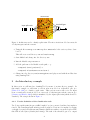
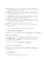
Learning-Tool : Analysing the
Computational Power of neural
microcircuits
Version 1.0
User Manual
c
2002
The IGI LSM Group
www.lsm.tugraz.at
June 11, 2006
This document is part of Learning-Tool Version 1.0
Copyright 2002 The IGI LSM group
Learning-Tool is free software; you can redistribute it and/or modify it under the terms of the GNU General Public
License as published by the Free Software Foundation; either version 2, or (at your option) any later version.
Learning-Tool is distributed in the hope that it will be useful, but WITHOUT ANY WARRANTY; without even the
implied warranty of MERCHANTABILITY or FITNESS FOR A PARTICULAR PURPOSE. See the GNU General
Public License for more details.
To get a copy of the GNU General Public License point your browser to http://www.gnu.org/copyleft/gpl.html.
The IGI LSM group
Institute for Theoretical Computer Science
Graz University of Technology
Inffeldgasse 16/b, A-8010 Graz, AUSTRIA
[email protected], www.lsm.tugraz.at
Contents
1 Introduction
3
1.1
What is Learning-Tool ? . . . . . . . . . . . . . . . . . . . . . . . . . . . . . .
3
1.2
About this manual . . . . . . . . . . . . . . . . . . . . . . . . . . . . . . . . .
3
1.3
Features of the current version . . . . . . . . . . . . . . . . . . . . . . . . . .
3
1.4
Getting and Installing Learning-Tool . . . . . . . . . . . . . . . . . . . . . . .
3
2 An Introductory example
4
2.1
Algorithm for offline training of the threshold gate . . . . . . . . . . . . . . .
5
2.2
Basic Concepts . . . . . . . . . . . . . . . . . . . . . . . . . . . . . . . . . . .
5
2.3
Implementation with Learning-Tool . . . . . . . . . . . . . . . . . . . . . . . .
6
3 Function reference
8
2
1
Introduction
1.1
What is Learning-Tool ?
Learning-Tool is a set of Matlab scripts that allows to asses the the real-time computing capability of neural microcircuit models. Learning-Tool is based on a new theoretical framework for
analysing real time computations in neural microcircuits: the Liquid State Machine (Sec. ??).
To get a thorough understandig of Learning-Tool it is a good idea to read the paper describing
the basic ideas[Maass et al., 2002] as well as the paper which describes on a higher level this
software package[Natschläger et al., 2002a].
1.2
About this manual
This manual is intended to describe how to use the Matlab scripts provided by Learning-Tool
to perform computer experiments within the LSM framework.
We assume that the reader has Matlab programming knowledge.
Although a short introtuction into the basic concept of the LSM (Sec. ??) is given we strongly
recommend to read [Maass et al., 2002, Natschläger et al., 2002b].
This manual is also available in HTML format either online via http://www.lsm.tugraz.
at/learning/usermanual or locally at your computer as file:<somepath>/lsm/learning/
documentation/usermanual/index.html if you have installed (unzipped) Learning-Tool in
the directory <somepath>.
1.3
Features of the current version
Matlab interface Learning-Tool is mainly written in Matlab and hence
Runs under Unix (Linux) and Windows
Object oriented design All the Learning Algorithms (Sec. ??), target functions (Sec. ??),
and readouts (Sec. ??) are implemented as Matlab classes.
Parallel Processing Usually the training of a readout (Sec. ??) involves many simulations
of the same microcircuit with different inputs and training of several readouts. This
can easily be run in parallel. Learning-Tool provides means to do this in a convinient
way (by employing the Parallel Matlab Toolbox [Svahn, 2001]).
1.4
Getting and Installing Learning-Tool
Learning-Tool is distributed under the GNU General Public License and can be downloaded
from http://www.igi.tugraz.at/learning.
To install Learning-Tool perform the following steps:
1. Donwload Learning-Tool from http://www.igi.tugraz.at/learning
3
microcircuit
threshold gate
input spike train
Figure 1: Architecture used to classify a spike train. The microcircuit is modeled as a network
of leaky-integrate-and-fire neurons.
2. Unzip the file learning-tool-VER.zip where VER stands for the version you have downloaded.
This will create a subdirectory lsm and lsm/learning
3. Start Matlab and change into the directory lsm
4. Run the Matlab script install.m.
5. Add the path lsm to the Matlab search path; e. g.
• addpath(’/home/jack/lsm’)} or
• addpath(’C:\Work\Neuroscience\lsm’).
6. Change into the directory lsm/learning/demos and play around with them. Have fun
using Learning-Tool !
2
An Introductory example
In this section we will introduce Learning-Tool by means of an introductory example. In
this simple example we will train a readout neuron modeled as a threshold gate (see
[Hertz et al., 1991]) to classify a spike train. This readout neuron will receive its input
from a neural microcircuit modeled as a network of leaky-integrate-and-fire neurons (see
[Gerstner and Kistler, 2002]) which is stimulated by the input spike train (which should be
classified). The setup is shown in Figure 1.
2.0.1
Precise definition of the classification task
Two Poisson spike trains (freqency 20 Hz, length 0.5 sec) are generated, and fixed as templates
0 and 1. The actual input spike train is generated as jittered versions of a template by varying
each spike by a random drawn amount (Gaussion distribuion with zero mean and a given STD;
this STD is called jitter (default jitter=4 ms)). The task of the threshold gate is to output
4
the number (0 or 1) of the (random choosen) template from which the input spike train was
generated.
2.1
Algorithm for offline training of the threshold gate
Here we just outline the main body of the procedure which we will use to train the readout.
This will be discussed in more detail in Section ??.
1. Define the neural microcircuit to be analyzed
2. Record spike responses of the neural microcircuit caused by different training inputs
drawn from an appropriate input distribution.
3. Convert the spike responses into states x(tk ) at various sample time points tk by some
low-pass filtering to get a somewhat smoothed signal. This mimics the effect of spike
transmission through a synapse to its postsynaptic neuron. This transformation can
also be dropped if one can cope directly with the spike response.
4. Apply a supervised learning algorithm to a set of training examples of the form h state
x, target-value yi to train a readout function f (a threshold gate in the case of this
example) such that the actual outputs f (x) are as close as possible to the target values
y given by the target function.
5. Evaluate the performance of the trained readout (i.e. the threshold gate) on an independent set of test inputs (which are usually drawn from the same distribution as the
training inputs).
2.2
Basic Concepts
The above description of the basic algorithm (Sec. 2.1) implicitly introduced all the basic
concepts we need to know to understand how Learning-Tool works:
Input Distribution The distribution from which the training (and test) inputs are drawn.
In our example the input distributio is defined byt the following simple procedure (for
fixed templates 0 and 1):
1. Randomly choose template 0 or 1
2. Add noise (jitter) to each spike in the template
Neural Microcircuit The circuit which receives the input and whos response is recorded
and analysed (in our example this a network of 135 leaky-integrate-and-fire neurons).
Response of the Microcircuit The response (output) of the neural microcircuit (in our
example the 135 spike trains produced by the microcircuit model).
State of the Microcircuit The transformed (smoothed) response (output) of the neural
microcircuit (in this examples this corresponds to a low-pass filtered (30 ms) version of
the spike trains). This transformation can also be dropped if one can cope directly with
the spike response.
5
Sample Time Points Since we can only handle finite sets of training examples we must
define time points at which we want to sample the state of the microcircuit (in this
example we will sample the states every 25 ms).
Readout Function A parameterized function/device which gets as input the circuit states
(or in some cases directly the circuit response) an computes the outputs of the system
(n this example a threshold gate).
Target Function/Filter A function which defines for each input time series the target
output time series of a readout function. In mathematical terms this should be a target
filter since we are talking about computations on time series.
Supervised Learning Algorithm By means of such algorithm the paramters of the readout — and only the readout — are adjusted such that the actual output of the readout
matches as close as possible the target output.
Training Set Set of inputs used to determine the parameter of the readout.
Test Set Set of inputs different to the training set which is used to asses the performance of
the trained readout.
As we will see each of this terms has its corresponding element within Learning-Tool .
2.3
Implementation with Learning-Tool
The full Matlab code is contained in lsm/learning/demos/spike train classification/spike class.m.
Defining the input distribution
Several input distributions are readly imlemented as Matlab objects.
The class
jittered templates (Sec. ??) provides the kind of input we need for our task. The followin code line generates a jittered templates object which produces single spike trains
from 2 patterns with a jitter of 4 ms:
InputDist = jittered_templates(’nChannels’,1,’nTemplates’,2,...
’Tstim’,0.5,’jitter’,4e-3);
Creating the neural microcircuit model
The following code generates a sparsely connected network of leaky-integrate-and-fire neurons.
The details of the network creation are the topic of the Circuit-Tool User Manual and thus
not described here.
% init the model
nmc = neural_microcircuit;
% add a pool of 135 leaky-integrate-and-fire neurons
6
[nmc,p1] = add(nmc,’Pool’,’origin’,[1 1 1],’size’,[3 3 15]);
[nmc,pin] = add(nmc,’Pool’,’origin’,[0 0 0],’size’,[1 1 1],...
’type’,’SpikingInputNeuron’,’frac_EXC’,1);
% connect the input to the pools/pools
nmc = add(nmc,’Conn’,’dest’,p1,’src’,pin,’Cscale’,0.9,...
’type’,’StaticSpikingSynapse’,’rescale’,0,’Wscale’,0.15,’lambda’,Inf);
% add recurrent connections within the pools
nmc = add(nmc,’Conn’,’dest’,p1,’src’,p1,’lambda’,2);
% define the respones (i.e. what to record)
nmc = record(nmc,’Pool’,p1,’Field’,’spikes’);
Creating the Training and Test inputs
Since we have defined the circuit model and the input distribution we can now simulate the
circuit with inuts drawn from this distribution an collect a training and test set. After the
simulations the spike responses are lowpass fitered and the states are samples every 25 ms.
% collect stimulus/response pairs for training
[train_response,train_stimuli] = collect_sr_data(nmc,InputDist,500);
% apply low-pass filter to spikes
train_states = response2states(train_response,[],[0:0.025:Tmax]);
% collect stimulus/response pairs for testing
[test_response,test_stimuli] = collect_sr_data(nmc,InputDist,200);
% apply low-pass filter to spikes
test_states = response2states(test_response,[],[0:0.025:Tmax]);
Setting up to train the threshold gate
Everything which has to do with the training of a readout is encapsulated in the class
external readout (Sec. ??). This object allows you to specify the target function (target filter) and the training algorithm (and several options for preprocessing). In our example
we use pseudo invers methode (implemented in the class linear classification (Sec. ??)
to determine the parameters of the threshold gate. The target function which outputs 0
(1) for all sample times (see definition of the task (Sec. 2)) is implemented in the class
segment classification (Sec. ??). Hence the code for setting up to train the threshold
gate is rather short:
readout{1} = external_readout(...
’description’,’with linear classification’,...
’targetFunction’,segment_classification,...
7
’algorithm’,linear_classification);
Do the training of the threshold gate
After everyting is set up properly we just need to start the training. Note that in the code
below the function function train readouts (Sec. ??) also measures the performance on the
tes set.
[trained_readouts, perf_train, perf_test] = train_readouts(...
readout,...
train_states,train_stimuli,...
test_states,test_stimuli);
Evaluation of the performance
After training we want to see how the network performs on indinivual test inputs:
plot_readouts(trained_readouts,test_states,test_stimuli);
3
Function reference
References
[Gerstner and Kistler, 2002] Gerstner, W. and Kistler, W. (2002). Spiking Neuron Models.
Cambridge University Press. See also http://diwww.epfl.ch/~gerstner/BUCH.html.
[Hertz et al., 1991] Hertz, J., Krogh, A., and Palmer, R. G. (1991). Introduction to the Theory
of Neural Computation. Addison-Wesley.
[Maass et al., 2002] Maass, W., Natschläger, T., and Markram, H. (2002). Real-time computing without stable states: A new framework for neural computation based on perturbations.
Neural Computation, 14(11):2531–2560.
[Natschläger et al., 2002a] Natschläger, T., Maass, W., and Markram, H. (2002a). The ”liquid computer”: A novel strategy for real-time computing on time series. Special Issue on
Foundations of Information Processing of TELEMATIK, 8(1):39–43.
[Natschläger et al., 2002b] Natschläger, T., Markram, H., and Maass, W. (2002b). Computer
models and analysis tools for neural microcircuits. In Kötter, R., editor, A Practical Guide
to Neuroscience Databases and Associated Tools, chapter 9. Kluver Academic Publishers
(Boston). in press.
[Svahn, 2001] Svahn, E. (2001). Parallel matlab toolbox: User documentation. Master’s
thesis, Chalmers University of Technology, Sweden. To get a copy of the toolbox contact
E. Svahn (email: [email protected], [email protected]) or get it via
ftp://ftp-at.e-technik.uni-rostock.de/pub/pm/.
8