1
AMS : An Integrated Simulator for Open Systems
Atika COHEN and Radouane MRABET
Université Libre de Bruxelles,
Service Télématique et Communication
Bd du Triomphe, CP 230 Brussels, Belgium
[email protected] and [email protected]
C=be; ADMD=rtt; PRMD=iihe; O=helios; S=cohen or S=mrabet
ABSTRACT The main objective of the OSISIM
project (Open System Integrated Simulator) is to set up
an atelier for the modelization of communication
networks and the analysis of their performances. The
atelier gives the end-user powerful tools to edit a
communication system in a graphical environment.
The representation of a system to be simulated is based
on models of several standard networks available in
the library which is the kernel of the atelier.
Each model implements uniform and well-defined sets
of functions, while having clearly specified interfaces.
This article describes the architecture of the atelier,
and focuses on the internal structure of basic models.
Introduction
The main objective of the OSISIM project is to set
up an atelier for the modelization of
communication networks and the analysis of their
performances. In the literature, we find the
description of different toolkits dedicated to this
field, as TOPNET [1], which is based on PROT
net, a class of Petri nets; NETMOD [2], which is
based on simple analytical models; BONeS [3],
which is based on block-oriented modeling
paradigm. On the other hand, our approach is
based on queueing networks.
Our atelier, named AMS (Atelier for Modelization
and Simulation), has to integrate the facilities and
the tools in such a way as to be easy to use by the
end-user. It gives the end-user some powerful
tools to easily edit a new communication system
in a graphical environment. The major facilities
are :
• basic library that includes the models of
several standard networks studied separately;
• tools for editing communication systems and
their characteristics;
• tools for visualizing simulation results;
• tools for simulation control.
The AMS will be based on the latest techniques in
software engineering such as : graphics,
windowing, pop-up menus and the object-oriented
programming paradigm. QNAP2 [6,7] (Queueing
Network Analysis Package 2) and GSS4 [8]
(Graphical Support System 4)1 are the main
software packages that will be used to operate the
AMS.
One component of this atelier is a library of basic
models including most of the standard networks
such as LANs (Ethernet, Token Ring, FDDI, etc),
WANs (X25, TCP/IP), satellite and radio
networks. It is obvious that the usefulness of the
atelier heavily depends on the number of available
models necessary to make up transmission
systems and networks.
The end-user of the AMS is not expected to be a
specialist in modeling or performance analysis;
however, he or she should be a communication
system designer. He or she will use the AMS to
build and validate an architectural choice, or to
compare several possible ways of solving a
problem.
Models have to be constructed in a very modular
fashion. That is why we have to build basic
models, which will make up other models of more
complex systems. Each basic model implements
uniform and well-defined sets of functions, while
having clearly specified interfaces.
This paper describes, in the first section, the
architecture of the AMS [4]. The second section
focuses on the internal structure of a basic model
[5], and the ways to reduce the code related to its
behavior.
I. Description of AMS
I.1. AMS architecture
Figure 1 shows the architecture of AMS. The
components of this architecture are arranged in
three principal groups : the objects that can be
manipulated by end-users (i.e. basic models) in
order to describe the communication system to be
1
These packages are trademarks of SIMULOG, a
French company specialized in the field of simulation.
simulated, the processes for editing and
generating code, and the set of files containing the
internal representation of the system under study.
Scenario_Element
Draw_Element
Scenario_Def
Arch_Draw
Arch
Descrip
Scenario
Descrip
Result_Element
Result_View
Basic Models
Result
Descrip
I.1.3 Files containing the description of the system
to be simulated.
Code_Generator
Simul
Descrip
Data +
Simulation
Control
Processor
Result
figure 1 : The architecture of the AMS
Hereafter follows
components.
a
description
c) Result_View : This process allows the end-user
to choose the types of simulation results he wants.
d) Code_Generator : This process generates the
code that describes the modelization of the global
system by means of the elements edited by the
end-user. This code is mainly written in the
QNAP2 language. The efficiency of this code
depends upon the internal structure of the basic
models. Before the code is generated, the validity
of the whole system is checked.
e) Processor : This process compiles and executes
the generated code. It requires the description of
the simulation experiment which includes a
number of data for simulation control (example :
simulation time length).
of
these
I.1.1 Objects manipulated by the user
a) Basic Models : The core of the AMS is the
library of basic models. A basic model is mainly a
communication entity such as a standard network,
protocol, gateway, etc. Each basic model is
characterized by a definite number of parameters
and an exhaustive list of measurements; in fact,
only a sub-list is provided by default.
In order to facilitate the use of these models, their
interconnection and their maintenance, a unified
internal architecture for basic models is defined
(see the following section) and used to structure
each of them.
b) Draw_Elements : Design objects for basic
models interconnection.
c) Scenario_Elements : These objects define the
scenario which will be followed during the
simulation.
d) Result_Elements : These objects define the
type and the form of results the end-user wants to
obtain after the simulation.
I.1.2 AMS processes
a) Arch_Draw : It is the process that allows the
end-user to edit his system graphically. It
generates the description of the edited system. The
validity of the system is checked during the
edition such as the connectivity between basic
models.
b) Scenario_Def : This process helps the end-user
to define the scenario he has chosen.
a) Arch_Descrip : A file which contains the
description of the system edited. This file is
generated by the Arch_Draw process.
b) Scenario_Descrip : This file contains the
functional description of the simulation steps. It is
generated by the Scenario_Def process.
c) Result_Descrip : This file contains the
description of the results. It is generated by the
Result_View process.
d) Simul_Descrip : This file contains code that
describes the modelization of the whole system. It
is generated by the Code_Generator process.
e) Results : This file corresponds to simulation
results The results are presented under the form
specified by the end-user
I.2. Functional description of AMS
The AMS is composed of four processes which
are Arch_Draw, Scenario_Def, Result_View and
Code_Generator. These processes, except the last
one, execute their codes in parallel. They
manipulate the files described above concurrently.
Let us describe how an end-user works with the
AMS. First of all, he executes the Arch_Draw
process. Using the basic models and the
Draw_Element, he prepares the system to be
modeled. For each basic model, he can modify the
predefined values of parameters while taking into
account the variation limits of the parameters.
With regard to measurements, the end-user can
either just ask for the default list of measurements,
or, for specific measurements he can choose from
the exhaustive list.
When the description of the system is complete,
he executes the Scenario_Def process, and uses
Scenario_Element to elaborate different scenarios
based on the parameters of the basic models. He
also executes the Result_View process in order to
determine the results he wants in accordance with
the measurements of each basic model.
Behavior Engine
Interface 1
The end-user can call these processes in any
order. The process Code_Generator can be called
only if all the elements required to generate the
code are edited.
Calling the Code_Generator process blocks up the
three other processes. It is going to validate the
different editions done by the end-user. If the
process detects some contradiction or omission, it
signals to the end-user what the problem is, stops
its execution, and releases the three other
processes, in order to allow the end-user to correct
or complete his description.
To launch the simulation the end-user has to
execute the processor.
II. Basic Models
II.1 Internal structure of basic models
Each basic model is to be detailed so as to reflect
its exact behavior. Hence, we have to specify the
functions performed by the basic model as exactly
as possible. Hereafter, basic models will be called
Detailed Basic Models (DBMs). The primary
advantage of this approach is to have accurate
measurements and to highlight the largest possible
number of parameters to characterize the system.
As a rule, a DBM can't be used alone, it must be
connected with one or several other DBMs, in
order to make up a complex system. That's why
each DBM needs one or more interfaces so as to
be connected to other DBMs.
Figure 2 shows the structure of a DBM code.
There are three blocks : Behavior Engine (BE),
Interfaces (Int) and Measurement Block (MB).
In the BE block, we find a modelization of the
behavior of the DBM. The behavior is controlled
by a set of parameters so that the end-user can
choose the values he wants to allocate to each
parameter.
Interface 2
Interface N
Measurement Block
figure 2 : Internal structure of a DBM code
A DBM can have several interfaces, N in figure 2.
That number N can either be a fixed value known
during the modelization phase (for instance, an
optical fiber cable can connect two workstations
and therefore N=2); or N can vary so that the
modeler can specify only the minimal and the
maximal values (for instance, an Ethernet cable
can connect several workstations).
The validity of the interconnection between
several DBMs is not checked by the DBMs
themselves but with tools belonging to the AMS.
Figure 3 shows how an interface, using messages,
reacts with its BE and with the outside world (i.e.
another interface belonging to another DBM).
Another
DBM
I
n
t
e
r
f
a
c
e
Behavior
Engine
DBM
figure 3 : A DBM with its BE and one Interface
Figure 4 represents a standard interface with its
two internal queues. Qio receives messages from
the outside, to be sent later to the BE. Qii receives
messages from the BE to be sent later to another
DBM which it is connected to.
Qii
BE
Another
DBM
Qio
figure 4 : A standard interface
Seen from the outside, all the interfaces are
similar but they differ in the way they interact
with their BEs. An interface doesn't play any
active role, its main function is to convey
messages from a BE to the outside and vice versa.
Each DBM has an identifier on which we find the
exhaustive list of parameters and their default
values, the measurement list, and a few text lines,
summarizing the main functions of the DBM.
II. 2 Reduced Basic Models (RBM)
Each basic model is to be detailed so as to reflect
its exact behavior. Namely, the functions
performed by the basic model are to be specified
as exactly as possible. The reasons why we have
chosen this approach are that we want :
• to have a model behavior close to a real
behavior;
• to derive accurate measurements from the
simulation runs.
However, this approach has some drawbacks
because of the large size of the code resulting
from the description of the DBM. These
drawbacks are :
• the compilation is very time consuming;
• the simulation is also very time consuming;
• the code describing a system is, of course, very
long, because the system is composed of
several DBMs, each of them having a long
code;
• during the simulation run, a large-sized
memory is needed;
• the end-user will be submerged with details, so
that his work for editing will be difficult.
In order to soften the effects of these drawbacks,
we suggest reducing the DBM code, by
eliminating, for example less significant details.
The code so obtained will be called RBM for
Reduced Basic Model. To do this, we are faced
with new problems, such as :
• how can less significant details be chosen ?
• during the construction of the system code, the
question that arises is : for which component is
the DBM required ? and for which one is the
RBM sufficient ?; the choice may be made
even more difficult, because each DBM can
have several RBMs associated to it.
The primary drawback of reducing DBMs is that
the simulation measurements are less accurate,
because the RBMs do not reflect the whole
behavior of the real system. An RBM has the
same internal structure as a DBM.
There are several methods to reduce a DBM code,
some of them are presented hereafter :
II.2.1. Physically reducing the size of the code
In order to reduce the size of a code, each DBM
will have several parts of its code deleted
physically. These parts may represent more or less
significant parts of the whole behavior, yet,
deleting them does not significantly change the
behavior, in so far as the remaining code is still
coherent.
Remarks:
• Unless deleting a part of the behavior entails
deleting the measurements associated with that
part, the end-user is not aware of the existence
of RBMs and DBMs, all that he knows, is that
there are basic models.
• The same DBM code can be broken down into
several RBMs, depending on which part is to
be deleted. That is why the DBM code has to
be analyzed carefully prior to deleting
anything.
For the deletion to be efficient, the DBM code
must be written in such a way as to facilitate this
task. In other words, the different parts of the
DBM behavior must be coded in a modular
fashion and be easily identifiable.
II.2.2 Logically reducing the size of the code
With this method, no part of the DBM's code is
deleted physically but some parts of it will not be
executed when the simulation is running.
The model builder (modeler) adds a set of
predicates in the DBM's code. Each predicate
governs a part of the code and when this predicate
is true, the code associated with it will be
executed, whereas if this predicate is false the
code related to it will not be run.
Each predicate is a combination of elementary
conditions : let C=(c1, c2,...,cn) be the elementary
conditions vector, with ci equal to 1 or 0, and
P=(p1, p2,..., pm) the predicate vector with pi=f(C),
i=1, 2,..., m, fi is a logical function using
operators such as AND, OR, NOT, etc. We can
have 2n different vectors C and k vectors P with
k≤ 2min(n,m). We can have k different versions of
the DBM code.
II.2.3. Using assumptions to simplify the DBM
code
The third method consists of simplifying the
DBM's code by making assumptions aimed at
reducing the complexity of some algorithms
which describe the behavior. This can be done by
physically replacing the complex algorithms with
other less complex ones.
II.2.4. The problems which arise when we want to
reduce DBMs
The following choices have to be made by a
competent modeler who has to decide which part
of code is to be deleted, which algorithm is to be
replaced, etc. Besides, he has to determine which
parts of the DBM's code significantly influence
the performance and which do not.
To achieve this, the modeler can be helped in
three ways : either by experts in the field of
network communications; or by researchers'
theoretical and experimental studies; or he can
make a simulation, called local simulation, for a
specific DBM, possibly interconnecting it to the
minimum number of DBMs required to have a
coherent system.
The modeler will often use the hybrid method
(when several methods are used to reduced one
DBM) because it gives him much flexibility, but
this flexibility involves building several RBMs
from the same DBM. This proliferation of RBMs
entails several problems which are fairly hard to
resolve. The first problem can be phrased as
follows : "Given a DBM to be reduced, which
RBM will serve as a substitute ? ".
II.3. Generic Models (GeMs)
In order to classify basic models, we define what
we call the Generic Models (GeMs), which are
model classes. Each Basic model belongs to one
or several GeMs according to the functionalities
which it handles. This classification will allow us
to use a tool to verify the validity of a system
edited by the end-user of the AMS.
The classification of the basic models will be done
on the basis of several criteria, for instance, the
largest possible number of links between one
basic model and the other ones; the OSI stack
layer a basic model belongs to; the fact that a
basic model is terminal or not, namely generating
or consuming messages.
Conclusion
The paper describes briefly the atelier AMS,
designed to evaluate the performance of open
systems. It comprises a library of basic models.
An internal structure is proposed for these models.
The description of a basic model have to be
reduced, in order to diminish the impact of some
drawbacks such as the CPU time and memory
size. These drawbacks appear when the system
under study is more or less complex.
References
[1] M. A. Marsan, G. Balbo, G. Bruno, F. Neri,
"TOPNET : A Tool for the Visual Simulation of
Communication Networks". IEEE Journal on Selected
Areas in Comm., Vol. 8, no 9, 1735-1747, Dec. 90.
[2] D. W. Bachmann, M. E. Segal, M. M. Srinivasan,
and T. J. Teorey, "NetMod: A Design Tool for LargeScale Heterogeneous Campus Networks", IEEE
Journal on Selected Areas in Comm., Vol. 9, no 1,
1735-1747, pp 15-24, January 91.
[3] K. S. Shanmugan, V. S. Frost, W. LaRue, "A
block-Oriented Network Simulator", Simulation, 8394, February 92.
[4] A. Cohen and R. Mrabet, "AMS : Atelier for
Modeling and Simulation", Internal Report,
IIHE/HELIOS-B-113-92, August 1992.
[5] A. Cohen and R. Mrabet, "AMS : Internal structure
for Basic Models", Internal Report, IIHE/HELIOS-B115-92, October 1992.
[6] "QNAP2 User's Manual", Simulog S.A. 1992.
[7] "QNAP2 Reference Manual", Simulog S.A. 1992.
[8] "GSS4 User's Guide", Simulog S.A. 1992.
II.4. Local and Global Measurements
Acknowledgments
As we said earlier, each basic model is
characterized by an exhaustive list of
measurements, called local measurements (LMs).
A default list is also defined for each basic model.
In general, the defaults lists are defined in the
same manner for all basic models and contain
typical measurements which are related to the
information handled by basic models or to the use
of a basic model.
Although typical measurements are defined in the
same way, they are processed differently because
basic models behave in different manners.
We wish to express our gratitude to SAIT
Electronics with whom we are colaborating on the
OSISIM project. We also gratefully acknowledge
the financial support granted by IRSIA.
The end-user is not only interested in LMs, but
also in measurements related to the whole system
which (s)he has edited. These measurements are
called the global measurements (GMs). The AMS
gives the end-user the means to define a GM in
function of LMs, but the semantic of the GMs has
to be defined by the end-user, except for some
verifications which are done by the AMS in
accordance with the type of LMs.