Download postscript (gz) - Artificial Intelligence Group

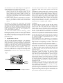
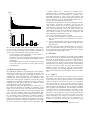
Combining Shallow Text Processing and Machine Learning
in Real World Applications
Günter Neumann
DFKI GmBH
Stuhlsatzenhausweg 3
66123 Saarbrücken
Germany
Abstract
In this paper, we present first results we
achieved and experiences we had combining
shallow text processing methods with machine
learning tools. In two research projects, where
DFKI and industrial partners are involved, German real world texts have to be classified into
several predefined categories. We will point out
that decisions concerning questions such as how
deep the texts have to be analysed linguistically
and how ML tools must be parameterized are
highly domain and data dependent. On the other
hand, there are some constants or heuristics
which may show in the right direction for future
applications.
1 Introduction
The world-wide exponential growth of information
brings along the need of tools helping not to loose a
general overview. In industry categorial systems in which
documents are classified according to themes are often
used. This helps to organize information and handle it
much more efficiently. Most of the time the classification
process itself is done manually which brings about enormous costs both time- and moneywise. Therefore automatic classification systems are very desirable. These
systems work mainly in two directions. The first direction makes extensive use of natural language processing
tools bringing about high costs in analysing and modelling the application domain but on the other hand promising a very high classification recall/precision value or
accuracy. The second direction makes use of statistical
methods such as machine learning promising low costs at
the expense of a lower accuracy. The idea now is to
combine both methodologies in the following way. A
shallow text processing (STP) system first extracts main
information from texts, then a machine learning (ML)
tool either tries to generalize this information for each
category and to build a representation for this, i.e. rules
or decision trees or simply stores this information and
uses distance measures in order to classify new texts.
In this approach several questions come to mind:
Sven Schmeier
DFKI GmBH,
Stuhlsatzenhausweg 3
66123 Saarbrücken
Germany
1) How deep do we have to analyse texts ?
2) Which learning algorithm is the best and how many
training examples do we need ?
3) What can we expect for resulting accuracy ?
There is one answer to all these questions:
It all depends on the data but our results give some heuristics and hints that might help in other application domains.
1.1 Shallow Text Processing Sof tw are
Linguistically based preprocessing of text documents is
performed by SMES, an information extraction core
system for real world German text processing [Neumann
et al, 1997]. The basic design criterion of the system is
to provide a set of basic powerful, robust, and efficient
natural language components and generic linguistic
knowledge sources which can easily be customized to
process different tasks in a flexible manner. The essential
abstract data types used in SMES are:
- dynamic Tries1 for lexical processing:
Tries are used as the sole storage device for all sorts of
lexical information (e.g., for stems, prefixes, inflectional
endings). Beside the usual functions (insertion, retrieval,
deletion), a number of more complex functions are available, most notably a regular Trie matcher, and a robust
recursive Trie traversal which supports recognition of
(longest matching) substrings. The latter is the basic
algorithm for on-line decomposition of German compounds.
- weighted finite state transducers (WFST):
WFST are used in order to represent cascades of grammar modules, e.g., proper name grammars (e.g. organizations, complex time/date expressions, person names),
generic phrasal grammars (nominal and prepositional
phrases, and verb groups) and clause level grammars.
Using WFST supports efficient and robust representation
of each individual grammar modul. Fig1 displays the
overall architecture of the SMES system.
1
A Trie (also known as letter tree) is an tree-based datastructure for efficiently storing common prefixes of words [Aho et
al, 1982].
Shallow Text
Processor
Lexical DB
> 120.000
stems;
> 12.000 verb
frames;
special
name lexica;
Tokenization
Text
Lexical processor
• Morphology
• Compounds
• Tagging
Grammars (FST)
general (NPs,
PPs, VG);
special (lexiconpoor,
Time/Date/Names)
;
general sentence
Chunk Parser
• phrases
• sentences
• gram. fct.
Set of
(partial)
parse trees
Fig1
It consists of two major components the Linguistic
Knowledge Pool (LKP) and STP, the core shallow text
processor of SMES. STP consists of three major components:
1) text tokenizer:
Each file at first is preprocessed by the text scanner.
Applying regular expressions, the text scanner identifies
some text structure (e.g., paragraphs, indentations),
word, number, date and time tokens (e.g, “1.3.96”,
“12:00 h”), and expands abbreviations. The output of the
text scanner is a stream of tokens, where each word is
simply represented as a string of alphabetic characters
(including delimiters, e.g. “Daimler-Benz”). Number,
date and time expressions are normalized and represented as attribute values structures. For example the
character stream “1.3.96” is represented as “(:date ((:day
1)(:mon 3)(:year 96)”, and “13:15 h'' as “(:time ((:hour
13)(:min 15)))”.
2) lexical processor:
Each token that has been identified as a potential wordform is lexically processed by the lexical processor.
Lexical processing includes morphological analysis,
recognition of compounds, retrieval of lexical information (where retrieval supports robust processing through
component based substring matching), and tagging that
performs word-based disambiguation.Text scanning is
followed by a morphological analysis of inflections and
the processing of compounds. The capability of efficiently processing compounds is crucial since compounding is a very productive process of the German
language. The output you receive after the morphological
analysis is the word form together with all its readings. A
reading is a triple of the form “(stem,inflection,pos)”,
where stem is a string or a list of strings (in the case of
compounds), inflection is the inflectional information,
and pos is the part of speech. Currently, the morpholgical
analyzer is used for German and Italian. It has an excellent speed (5000 words/sec without compound handling,
2800 words/sec with compound processing where for
each compound all lexically possible decompositions are
computed).
3) chunk parser:
The chunk parser is subdivided into three components.In
the first step phrasal fragments are recognized, like general nominal expressions and verb groups or specialized
expressions for time, date, and named entity. The structure of potential phrasal fragments is defined using
weighted finite state transducers (WFST). As a second
stage, the dependency-based structure of the fragments of
each sentence is analysed using a set of specific sentence
patterns. These patterns are also expresssed by means of
WFST. At the final step, the grammatical functions are
determined for each dependency-based structure on the
basis of a large subcategorization lexicon.
SMES has very broad linguistic knowledge source, i.e. a
huge lexical data base (more than 120.000 stem entries,
more than 12,000 subcategorization frames as well as
basic lexica for proper names). It has a broad coverage
of special subgrammars for recognizing unknow propername and general grammars for nominal, prepositional
and verb phrases. Complete processing of a text with 400
words takes about 1 second. Very important in the context of this paper is SMES's high degree of modularity:
each component can be used in isolation. Thus, it is possible to run only a subset of the components, e.g. to peform term extraction by using only the specialized subgrammars or/and the phrasal grammars.
1.2
Machine Learning Sof tw are
Several Machine Learning Tools, which stand for different learning paradigms, have been selected and evaluated
in different settings of our domains. First, we made use
of the MLC++ Library [Kohavi and Summerfield, 1996]
which contains several algorithms, i.e. ID3 [Quinlan,
1986], the mother of all decision tree based algorithms;
MC4 which combines ID3 and pruning methods of C4.5
[Quinlan, 1993]; IB [Aha, 1992], an Instance Based
Learner, equivalent to nearest neighbor learning. We
tried out the RIPPER Algorithm [Cohen, 1995] and its
boosted version, which both are rule learning algorithms.
We did not experiment with Naive Bayes [Langley et al
1992, Good 1965] algorithms2 because of our data format (see 2.1), this is one of our main focus in the current
research.
Other systems, such as ROCCHIO [Lewis et al, 1996] or
SVM-LIGHT [Joachims, 1998], have not been used yet
in our scenario because they produce only binary classi2
Our implementation of the Naive Bayes algorithm uses
wordfrequencies for computing propabilities.
fiers which have several disadvantages in our application
domain described by the following two points:
1) The number of classifiers is equal to the number of
classes you have in your category system. As we
plan the system to be an overnight learning system in
order to improve the system’s quality over time, we
depend on the statements of our future users whether
the system is fast enough to learn several classifiers
instead of only one.
2) There is also a problem in determining a representative set of negative examples for one category3
Maybe a great number of tests will be needed to find
this set.
The clerk then just selects one or more of the proposed
possibilities, adds some flowery phrases and sends the
reply.
In SCEN2 we intend to build a more “classical” textcategorization system which associates press releases with
several categories without human interaction. Both scenarios consist of the same general system architecture
(Fig.2). In an offline step, texts from an example corpus
are passed through our STP module. Its output is then
fed to the ML module which creates the categorizer
(CAT). In the online step, new texts are again passed
through the STP module, its output is given to the CAT
which returns the –hopefully right- category.
Nevertheless we expect new corpus data that should
solve the second problem concerning the number and the
distribution of training examples over the categories. The
first point can only be solved or answered in the beta
testphase (to be started in September 1999) by the future
users. Nevertheless we plan our next experiments to
cover binary learning systems too.
We also tried neuronal network technology, SNNS
[Zell,95] but neuronal networks need too much adjusting
knowledge especially if there are many input neurons
(the number of features in the input vector) and many
output neurons (the number of categories). So we didn’t
pursue this route.
2.1 Data
2
Application Areas
We use the STP and ML techniques in two different
industrial research projects. In SCEN1 -ICC (Innovation
at the Call Center)- we built an assistance system helping
a clerk in a call center with answering questions of a
customer. In this call center answers are not formulated
spontanously but they consist of preformulated texts
which are associated with certain categories. These categories are comparable to a category system used in faq
lists. The system’s task is to assign new incoming emails
to one or more categories and to propose the preformulated answers.
Fig2
OFFLINE
vector
text
STP
ML
creates
vector
CAT
category
ONLINE
3
The numbers of positive and negative examples should not
differ too much.
The kind of data is essential for STP and ML systems.
For STP, the depth of analysis depends very much on the
quality of the data. This means that if for example the
scanner makes use of punctuation marks to seperate one
sentence from another, we must be sure that these marks
are set at the right places. Furthermore recognizing
whether a point indicates an abbreviation or the end of a
sentence is not a trivial task. Morphological information
about words is dependent on the lexicon used so we must
be sure that the words used in the texts are covered by
our lexicon. Further parsing can only succeed if the texts
are formed according to grammatical rules or if the
parser is very robust.
In our examples, the texts in SCEN2 are of a much better
quality than the texts in SCEN1. In emails, punctuation
marks are used very loosely, we have to cope with a
large amount of misspellings and most emails lack
grammatical correctness. See the following example:
“ Wie mache ich zum mein Programm total deinstalieren,
und wieder neu instalierem, mit, wen Sie mir senden
Version 4.0 ??????????????” which roughly translates
to: “How do I make to mine program totally deinstal, and
again new reinstall, with, who you send to me version 4.0
??????????????”.
Here we have problems with wrong placed commas,
misspellings (which can hardly be solved by fuzzy
matching methods) and the whole sentence is grammatically incorrect (but understandable for persons). In general, the decision on how deep you will do linguistic
preprocession depends on the data (because of the pure
recall expected). If you go too deep you might not get
any results, whereas if you decide to stay on the surface,
you will probably get problems in detecting structural
similarities in data.
Switching over to the ML part, two main issues come
into mind: the number of categories and training examples available (and their distribution among the categories) and the length of the texts.
In SCEN1 there are 2350 training examples and 44 categories (see Fig3 for distribution). The emails contain 60
words on average. In SCEN2 there are 824 training examples and 6 categories (see Fig4 for distribution). The
press releases contain 578 words on average.
Fig3
# E x a m p le s
300
250
200
150
100
50
C a ts
0
Fig4
350
# E x a m p le s
300
250
200
150
100
50
0
1
2
3
4
5
6
C a ts
We will see that these information have important effects
on our results. One last point to mention concerns the
noisyness of data. It turned out that the data of SCEN1 is
noisier than that of SCEN2 in the following sense:
- in some emails several problems are mentioned, i.e.
several categories are appropriate
- the category system is ambigous by offering several
classes for the same problems (highlighting several
subthemes)
- the example corpus has been “created” by the clerks
in the call center and has not been supervised by
some expert(s).
2.2 Data Preprocessing
We studied the influence of non linguistic and linguistic
preperation on data that is fed to the ML programs. We
tried simple letter trigrams, morphological analysis of
substantives, verbs and adjectives, and shallow parsing
methods that extract domain specific information. The
main issue of the “deeper” linguistic preprocessing is the
combination of domain knowledge with pure statistical
methods of the ML part so that we are enabled to avoid
counterproductive rules resp. branches.
We studied the effects of different input vector sizes i.e.
the connection between the number of attributes in the
input vector and the texts and expected the following
relationship: the more data you have and the longer each
text is the more attribute values you should expect. Besides, the use of letter trigrams should enlarge the number of attribute values compared to stemming. However
you have to make sure that you do not to run into problems associated with overfitting. So far there is very little
agreement on which circumstances determine the length
of vectors. Therefore we made several experiments with
a smaller dataset, e.g. 5 categories in SCEN1 and a
smaller amount of examples in SCEN2 to get a clue to
the borders where we could expect a, possibly local,
maximum of accuracy. This was the case between 300
and 1000 attributes for SCEN1, and 500 to 6000 attributes for SCEN2. If we go beyond these borders the accuaracy of the performance will decrease.
Furthermore we decided not to use wordfrequency measures because –especially in SCEN1- the texts are not
long enough and we do not have enough examples to
concatenate several texts. So the ML algorithms have to
learn “keyword-spotting” rules resp. trees. Notice that
extracted tokens have to be reordered in the way that the
same tokens occuring in the texts are assigned to the
same attributes in the feature vectors.
Two ways of reordering come into mind:
1) Use the extracted tokens as attribute names and assign a positive value to this attribute if it occurs in
the text.
2) The second algorithm uses the extracted tokens as
attribute values and reorders them according to their
apperearences.
In general both algorithms should produce the same results, we used the second way which gave us the possibility to determine the “degree of generalization”4 simply
by changing the length of the vector.
3
Results
Now we present our sometimes surprising results ordered
by scenario, kinds of preprocessing and ML algorithms.
The kind of measurement is “accuracy” which means in
average X percent of incoming new texts will be classified into the right category. We preferred this kind of
measurement to classical precision/recall measurements
because it provides a better overview. We consider it is
difficult to have any idea of what 44 precision/recall
values of SCEN1 say about the usefullness of the system.
All measurements were done using 10 fold cross validation.
3.1
SCEN1
The results we achieved in this project seem to be very
bad at first sight. This is due to the fact that the category
system does not clearly seperate emails. This means an
email can belong to more than one class. As we build an
assistance system we do not only take positive solutions
into account that are proposed to be the right category
with the highest propability but we go down to solutions
that are above some threshold. This threshold is defined
as follows: During the learning phase we build a confusion matrix, i.e., for each test and for each category the
decisions of the categorizer are documented and entered
into a table. Each line in this table represents all documents belonging to one category, the values in this line
denote the associated classes by the categorizer. In
SCEN1 we noticed a close relation between the right
4
i.e., determining a token to be unimportant for a class.
categories and the most frequent chosen “wrong” classes.
In most cases these classes form a superset of the missing
categories needed for multi-class problems which is acceptable for the users. Unfortunately we have not found a
way expressing this fact directly in our accuracy values.
Empiric measurements tell us that we should add about
20 percent accuracy to each outcome.
3 . 1 . 1 Letter Trigrams
We start our test series with letter trigrams. This means
you take a window of three letters and shift it over the
whole text. For each position you get a token which is
appended to the ML input vector.
So the sentence “John loves Mary” expands to (“Joh”
“ohn” “hn “ “n l” “ lo” ......).
Now the results:
IB
ID3
MC4
RIPPER
Boosted R
300
500
28.12
25.12
25.23
41.09
49.39
30.58
27.27
26.65
44.72
50.03
1000 Number of
Attributes (#A)
27.28
28.93
28.93
46.54
51.98
We observed that if we increase the number of attributes
beyond 1000 the accuracy values would dercrease. We
have tested several different vector sizes (600, 750, 900
attributes) just for boosted RIPPER but we never got
over 52.5 %.
3 . 1 . 2 M o rpho lo g ica l Ana ly sis
In this test we removed all the words except unknown
words5, nouns, verbs, adjectives and adverbs. Additionally only the stems of the remaining words – of course
unknown words were not stemmed - were put into ML
input vector.
IB
ID3
MC4
RIPPER
Boosted R
300
500
1000 #A
31.85
46.01
46.96
52.03
54.76
37.01
46.52
46.43
55.97
58.31
38.15
46.48
46.44
53.95
56.11
This testseries show that in order to analyse short German texts stemming seems to a better choice than simple
trigramming. In our opinion this is due to the fact, that
the German language has got many different word forms.
Furthermore we see that it is not always advantagous to
enlarge the number of the vector’s attributes too much
without considering which ML algorithm is used. Again
the difficulty is to find out which is the optimal length.
3 . 1 . 3 Sha llo w Pa rsing
We now switch over from morphological analysis to
shallow text processing. This means that by adding domain specific knowledge to the process we shift from the
pure statistic approach to a more knowledge based approach. What we have to do now is to detect the main
information inside the texts. We found out the main information of the texts in SCEN1 is to be found in sentences containing negation and special words as well as
in questions. We extract such information and add it to
the vectors of the previous chapter simply by adding a
special character to the words found in these sentences
(this method has to be refined and we expect better results by using more suitable representations):
IB
ID3
MC4
RIPPER
Boosted R
300
500
1000
22.09
41.17
41.90
49.17
51.12
25.55
42.05
43.12
56.90
59.64
27.01
43.45
44.09
56.14
59.09
#A
We see some very surprising results. Although the first
four ML algorithms performed worse compared to the
previous experiment, RIPPER and its boosted version are
slightly improved. The reason for this behaviour has to
be explored in future work.
3.2
SCEN2
In contrast to the results in SCEN1 we now obtain concrete results which prognose the future behavior of the
system because we are only interested in the categorizer’s favourate category per example data. Again we
begin with letter trigramming and go on to morphological anlysis. We didn’t proceed to deeper STP yet but we
intend do this in future researches. Remember we now
have only 6 categories and rather long, well formulated
texts.
3 . 2 . 1 Letter Trigrams
Again our first test consists of trigramming the texts and
developing the input vectors from these values. We
achieve the following results6:
IB
ID3
MC4
RIP
BoR
500
1000 2000 3000 4000 5000 6000
74.74
70.66
69.69
68.19
75.10
76.05
71.85
69.69
69.74
76.09
76.92
72.01
70.21
69.98
76.12
76.75
71.65
68.71
70.12
76.43
77.01
error
error
68.43
75.98
75.71
error
error
68.89
75.46
75.12
error
error
68.22
75.89
5
Due to the very large lexical source we can expect that unknown words are either domain specific expressions or spelling errors.
6
ID3 and MC4 ran out of memory on our Sparc Ultra 4 with
4 cpus and 4096 mByte RAM.
Notice that the results are a lot better in this scenario
than in SCEN1. This is so mainly because of the smaller
number of categories and the kind of categories as they
ar not overlapping.
3 . 2 . 2 M o rpho lo g ica l Ana ly sis
As in SCEN1 we analyse the texts morphologically and
filter out all words except unknown words, nouns, verbs,
adjectives and adverbs. The results are:
IB
ID3
MC4
RIP
BoR
500
1000 2000 3000 4000 5000 6000
68.78
68.10
67.42
66.23
78.42
67.93
70.44
68.32
66.83
78.66
67.38
75.24
71.04
66.37
79.14
67.92
72.84
70.36
69.18
79.14
67.33
error
error
69.22
79.22
68.05
error
error
69.78
78.78
68.73
error
error
68.56
79.43
Also in this scenario we see that morpholgical analysis
raises the overall performance. Again we see the reason
for this in the great numbers of different wordforms in
the German language.
A second very interesting result is the huge jump of increasing accuracy by using the boosted version of
RIPPER. It seems that with longer texts we have a massive amount of overgenerated rules or branches which
turn out to be very contraproductive. This point too, is an
unsolved secret so far.
4
Summary and Outlook
In this paper we presented a system for text categorization consisting of a combination of a STP module and
different ML algorithms and evaluated its performance
for two different scenarios. We showed many results,
attempts to explain them and some unsolved problems,
too. We pointed out that different scenarios need different processing methods and learner parameterizations to
get the best results. We also saw two constant factors:
1) Linguistic based preprocessing raised the system’s
overall performance in both scenarios. We also think that
in particular shallow text processing with its high degree
of robustness and efficiency is an appropriate means to
combine domain knowledge with statistical categorization algorithms.
2) The boosted version of RIPPER promises the best
results even under different data preprocessing circumstances. We do not claim that this algorithm works best
in general but it worked best compared to the ML algorithms chosen in our scenarios.
Our future work will concentrate on both, the linguistic
and the statistic modules, i.e., we will define more domain specific parsing rules and we will experiment with
further ML algorithms, for example the first order version of RIPPER namely FLIPPER, or WHIRL [Cohen,
1998].
References
[Aha, 1992] David W. Aha. Tolerating noisy, irrelevant
and novel attributes in instance based learning algorithms. International Journal of Man-Machine Studies,
36(1):267-287, 1992
[Aho et al., 1982] Alfred V. Aho, John E. Hopcroft,
Jeffrey D. Ullman. Data Structures and Algorithms
1982: Addison-Wesley
[Cohen, 1995] William W. Cohen. Fast Effective Rule
Inductionl In ML95, 1995
[Cohen, 1998] William W. Cohen. Joind that generalize:
Text Classification Using WHIRL .In KDD-98.
[Good, 1965] I.J. Good. The Estimation of Probabilities.
An Essay on Modern Bayesian Methods. MIT-Press,
1965
[Joachims, 1998] Thorsten Joachims. Text Categorization with Support Vector Machines. European Conference on Machine Learning (ECML),1997
[Kohavi and Sommerfield, 1996] Ronny Kohavi and
Dan Sommerfield. MLC++ Machine Learning library in
C++. User Manual.
http://www.sgi.com/Technology/mlc
[Langley et al, 1992] P. Langley, W. Iba & K. Thompson. An analysis of bayesian classifiers. Proceedings of
National Conference on Artificial Intelligence. AAAI
Press and MIT-Press, 1992.
[Lewis, 1991] David D. Lewis. Evaluating Text Categorization. Proceedings of the Speech and Language Workshop, 1991
[Lewis et al, 1996] David D. Lewis, Robert Shapire,
James P. Callan and Ron Papka. Training Algortihms for
Linear Text Classifiers. SIGIR, 1996
[Neumann et al, 1997] G. Neumann, R. Backofen, J.
Baur, M. Becker, C. Braun. An Information Extraction
Core System for Real World German Text Processing. In
Proceedings of 5th ANLP, Washington, March, 1997.
[Quinlan, 1986] J.R. Quinlan. Induction of Decision
Trees. Machine Learning, 1:81-106, 1986.
[Quinlan, 1992] J.R.Quinlan. C4.5: Programs for Machine Learning. Morgan Kaufmann, Los Alto, California
, 1992.
[Zell, 1995] A. Zell et al. SNNS: Stuttgart Neural Network Simulator. IPVR - Applied Computer Science -Image Understanding, Report No. 6/95, 1995