Download CS 5604 Information Retrieval and Storage Spring

CS 5604 Information Retrieval and Storage
Spring 2015
Final Project Report
Feature Extraction & Selection, Classification
Project Members:
Xuewen Cui
Rongrong Tao
Ruide Zhang
Project Advisor:
Dr. Edward A. Fox
05/06/2015
Virginia Tech, Blacksburg, Virginia 24061, USA
1
Executive Summary
Given the tweets from the instructor and cleaned webpages from the Reducing Noise team, the planned
tasks for our group were to find the best: (1) way to extract information that will be used for document
representation; (2) feature selection method to construct feature vectors; and (3) way to classify each
document into categories, considering the ontology developed in the IDEAL project. We have figured out
an information extraction method for document representation, feature selection method for feature vector
construction, and classification method. The categories will be associated with the documents, to aid
searching and browsing using Solr. Our team handles both tweets and webpages. The tweets and
webpages come in the form of text files that have been produced by the Reducing Noise team. The other
input is a list of the specific events that the collections are about. We are able to construct feature vectors
after information extraction and feature selection using Apache Mahout. For each document, a relational
version of the raw data for an appropriate feature vector is generated. We applied the Naïve Bayes
classification algorithm in Apache Mahout to generate the vector file and the trained model. The
classification algorithm uses the feature vectors to go into classifiers for training and testing that works
with Mahout. However, Mahout is not able to predict class labels for new data. Finally we came to a
solution provided by Pangool.net [19], which is a Java, low-level MapReduce API. This package provides
us a MapReduce Naïve Bayes classifier that can predict class labels for new data. After modification, this
package is able to read in and output to Avro file in HDFS. The correctness of our classification
algorithms, using 5-fold cross-validation, was promising.
2
Table of Contents
I. Introduction ............................................................................................................................. 5
II. Literature Review ................................................................................................................... 7
1. Textbook ......................................................................................................................... 7
1.1 What is Classification? ........................................................................................... 7
1.2 Feature Selection ................................................................................................... 8
1.3 Naïve Bayes Classification ..................................................................................... 8
1.4 Vector Space Classification.................................................................................... 9
1.5 Support Vector Machine ........................................................................................10
2. Papers ...........................................................................................................................11
3. Tools and Packages.......................................................................................................12
III. User Manual.........................................................................................................................13
1. Attachment Description ..................................................................................................13
2. Usage of Package ..........................................................................................................13
2.1 Generate Mahout Naïve Bayes Classification Model .............................................13
2.2 Predict Class Label for New Data Using Mahout Naïve Bayes Classifier ..............14
2.3 Pangool: MapReduce Naïve Bayes Classification and Class Label Prediction ......14
IV. Developer Manual................................................................................................................16
1. Algorithms ......................................................................................................................16
1.1 Classification Algorithms in Mahout .......................................................................16
1.2 Classification Configuration ...................................................................................18
2. Environment Setup ........................................................................................................20
2.1 Installation.............................................................................................................20
2.2 Data Import ...........................................................................................................22
2.3 Upload Tweets and Webpages of Small Collection to Solr ....................................24
2.4 Load Webpages of Small Collection to HDFS .......................................................27
3. Naïve Bayes Classification .............................................................................................28
3.1 Transform Tweets to Sequence File and Feature Vector on Our Own Machine ....28
3.2 Commands for Classification with Mahout Naïve Bayes Algorithm ........................32
3.3 Applying Mahout Naïve Bayes Classifier for Our Tweet Small Collection ..............33
3.4 Using Mahout Naïve Bayes Classifier for Tweet Small Collections from Other
Teams.........................................................................................................................37
3.5 Generate Class Label for New Data Using Mahout Naïve Bayes Model................37
3.5 Using Pangool to Predict Class Label for New Data ..............................................41
4. Evaluation ......................................................................................................................44
4.1 Cross Validation ....................................................................................................44
4.2 Summary of Results ..............................................................................................44
V. Timeline/Schedule ................................................................................................................47
VI. Conclusion ...........................................................................................................................48
VII. Future Work ........................................................................................................................49
VII. Acknowledgements.............................................................................................................49
VIII. References ........................................................................................................................50
3
List of Figures
Figure 1: Solr Installation………………………………………………………………………21
Figure 2: Cloudera Virtual Machine Installation……………………………………………….22
Figure 3: Data CSV file modification example………………………………………………...23
Figure 4: Schema.xml modification example…………………………………………………..23
Figure 5: Import CSV file to Solr…………………………………………………………........24
Figure 6: Tweets and webpages uploaded to Solr……………………………………………...27
Figure 7: LongURLs from the new tweets…………………………………………………..…27
Figure 8: Nutch finished crawling the webpages………………………………………………28
Figure 9: Print out message from text file to sequence file…………………………………….29
Figure 10: Generated sequence file…………………………………………………………….30
Figure 11: Print out message from sequence file to vectors……………………………………31
Figure 12: Generated tf-idf results……………………………………………………………...31
Figure 13: Generate word count results………………………………………………………...32
Figure 14: Confusion Matrix and Accuracy Statistics from Naïve Bayes classification……….33
Figure 15: Error message when generating classification labels for new unlabeled test data….38
Figure 16: Using Mahout Classification Model and Additional Program to Predict Class Labels
of New Unlabeled Test Data……………………………………………………………………41
Figure 17: Example of Training Set…………………………………………………………….42
List of Tables
Table 1: Comparison between Mahout and non-Mahout approach……………………………..16
Table 2: Characteristics of the Mahout learning algorithms used for classification…………….17
Table 3: Options of Mahout feature vector generation………………………………………….19
Table 4: Results of Small Collections of Tweets………………………………………………..45
Table 5: Results of Large Collections of Tweets………………………………………………..45
Table 6: Results of Small Collections of Webpages…………………………………………….46
Table 7: Results of large Collections of Webpages……………………………………………..46
4
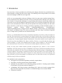
I. Introduction
Our team aims to classify provided tweets collections and webpage collections into pre-defined classes,
which ultimately can help with Solr search engine. The Reducing Noise team provided us the cleaned
tweets and webpages in HDFS for us to begin with.
At first, we are recommended to make use of Mahout, which is an open source machine-learning library.
For text classification task, Mahout will be able to help us encode the features and then create vectors out
of the features. It also provides techniques to set up training and testing sets. Specifically, Mahout can
convert the raw text files into Hadoop's SequenceFile format. It can convert the SequenceFile entries into
sparse vectors and modify the labels. It can split the input data into training and testing sets and run the
built-in classifiers to train and test. Existing classification algorithms provided in Mahout include: (1)
Stochastic
gradient
descent
(SGD):
OnlineLogisticRegression,
CrossFoldLearner,
AdaptiveLogisticRegression; (2) Support Vector Machine (SVM); (3) Naive Bayes; (4) Complementary
Naive Bayes; (5) Random Forests. We tried our collections with Naïve Bayes classification algorithm
since it is simple and very suitable for text classification tasks.
However, we find that Mahout Naïve Bayes classification algorithm is not able to predict class labels for
new data. This means that we can only generate Naïve Bayes classifiers but we are not able to label new
data. In order to solve this problem, we looked into available books and online tutorials and finally found
a package from “Learning Apache Mahout Classification” [20], which could be used to predict class
labels for new data using Mahout Naïve Bayes classifiers. However, we noticed that this package only
works for Hadoop 1.1.1 and is not compatible with our cluster, which is Hadoop 2.5. We tried to modify
the code and talk to the TAs, however, we did not successfully adapt this solution to our cluster.
Finally we came across another solution provided by Pangool.net [19], which is a Java, low-level
MapReduce API. This package provides us a MapReduce Naïve Bayes classification algorithm and it can
also predict class labels for new data. The most important thing is that this package is compatible with all
versions of Hadoop. This package is modified to be able to read in and write to Avro files in HDFS. We
used this package to generate Naïve Bayes classifiers for small collections of tweets and webpages, and
large collections of tweets and webpages, for different teams. We showed the accuracy of our generated
classifiers using 5-fold cross validations.
Our contribution can be summarized as:
 Investigation of classification algorithms provided by Apache Maout
 Naïve Bayes classifiers generated using Apache Mahout
 Prediction for class labels for new data using package provided in “Learning Apache Mahout
Classificaiton” [20], but only works for Hadoop 1.1.1
 A MapReduce Naïve Bayes package called Pangool [19], which can be used to generate Naïve
Bayes classifiers and predict for new data. It is modified to adapt to Avro format in HDFS.
 Evaluation of classfiers
5
Here is a list of what we are going to cover in the following sections. Section II gives an overview of
related literature. More about the packages used is given in Section III. Section IV chronicles our
development efforts. Section IV.1 gives an overview of Apache Mahout for classification. Section IV.2
gives our end-to-end handling of classification in conjunction with a small collection and searching with
Solr. Section IV.3.5 gives our ultimate solution for predicting classes using Pangool [19], following
discussion earlier in Section IV.3 about attempts to use Mahout. Section IV.4 describes evaluation tests.
Section V summarizes our schedule while Section VI summarizes our efforts and conclusions, leading to
Section VII which gives future plans.
6
II. Literature Review
1. Textbook
1.1 What is Classification?
From [15] chapter 13, we learn that many users have ongoing information needs. For example, a user
might need to track developments in multi-core computer chips. One method of doing this is to issue the
query multi-core AND computer AND chip against an index of recent newswire articles each morning.
How can this repetitive task be automated? To this end, many systems support standing queries. A
standing query is like any other query except that it is periodically executed on a collection to which new
documents are incrementally added over time.
If the standing query is just multicore AND computer AND chip, the user will tend to miss many relevant
new articles which use other terms such as “multicore processors”. To achieve good recall, standing
queries thus have to be refined over time and can gradually become quite complex. In this example, using
a Boolean search engine with stemming, the user might end up with a query like (multi core OR multicore) AND (chip OR processor OR microprocessor).
To capture the generality and scope of the problem space to which standing queries belong, we now
introduce the general notion of a classification problem. Given a set of classes, we seek to determine
which class a given object belongs to. In the example, the standing query serves to divide new newswire
articles into the two classes: documents about multicore computer chips and documents not about
multicore computer chips. We refer to this as two-class classification.
A class need not be as narrowly focused as the standing query multicore computer chips. Often, a class
describes a more general subject area like China or coffee. Such more general classes are usually referred
to as topics, and the classification task is then called text classification, text categorization, topic
classification, or topic spotting. Standing queries and topics differ in their degree of specificity, but the
methods for solving routing, filtering, and text classification are essentially the same.
Apart from manual classification and hand-crafted rules, there is a third approach to text classification,
namely, machine learning-based text classification. It is the approach that we focus on in our project. In
machine learning, the set of rules or, more generally, the decision criterion of the text classifier, is learned
automatically from training data. This approach is also called statistical text classification if the learning
method is statistical. In statistical text classification, we require a number of good example documents (or
training documents) for each class. The need for manual classification is not eliminated because the
training documents come from a person who has labeled them – where labeling refers to the process of
annotating each document with its class. But labeling is arguably an easier task than writing rules. Almost
anybody can look at a document and decide whether or not it is related to China. Sometimes such labeling
is already implicitly part of an existing workflow. For instance, the user may go through the news articles
returned by a standing query each morning and give relevance feedback by moving the relevant articles to
a special folder like multicore-processors.
7
1.2 Feature Selection
Feature selection is the process of selecting a subset of the terms occurring in the training set and using
only this subset as features in text classification. Feature selection serves two main purposes. First, it
makes training and applying a classifier more efficient by decreasing the size of the effective vocabulary.
This is of particular importance for classifiers that, unlike NB, are expensive to train. Second, feature
selection often increases classification accuracy by eliminating noise features. A noise feature is one that,
when added to the document representation, increases the classification error on new data. Suppose a rare
term, say arachno-centric, has no information about a class, say China, but all instances of arachno-centric
happen to occur in China documents in our training set. Then the learning method might produce a
classifier that wrongly assigns test documents containing arachno-centric to China. Such an incorrect
generalization from an accidental property of the training set is called over-fitting.
We combine the definitions of term frequency and inverse document frequency, to produce a composite
weight for each term in each document.
The tf-idf weighting scheme assigns to term t a weight in document d given by
tf-idft,d = tft,d × idft.
In other words, tf-idft,d assigns to term t a weight in document d that is
a. highest when t occurs many times within a small number of documents (thus lending high
discriminating power to those documents);
b. lower when the term occurs fewer times in a document, or occurs in many documents (thus offering a
less pronounced frequency relevance signal);
c. lowest when the term occurs in virtually all documents.
At this point, we may view each document as a vector with one component corresponding to each term in
the dictionary, together with a weight for each component that is given by the previous equation. For
dictionary terms that do not occur in a document, this weight is zero. This vector form will prove to be
crucial to scoring and ranking. As a first step, we introduce the overlap score measure: the score of a
document d is the sum, over all query terms, of the number of times each of the query terms occurs in d.
We can refine this idea so that we add up not the number of occurrences of each query term t in d, but
instead the tf-idf weight of each term in d.
1.3 Naïve Bayes Classification
The first supervised learning method introduced is the multinomial Naive Bayes or multinomial NB
model, a probabilistic learning method. The probability of a document d being in class c is computed as
P(c|d) ∝ P(c) ∏ P(tk|c) 1 ≤ k ≤ nd where P(tk|c) is the conditional probability of term tk occurring in a
document of class c. We interpret P(tk|c) as a measure of how much evidence tk contributes that c is the
correct class. P(c) is the prior probability of a document occurring in class c. If a document’s terms do not
provide clear evidence for one class versus another, we choose the one that has a higher prior probability.
8
⟨t1, t2, . . . , tnd ⟩ are the tokens in d that are part of the vocabulary we use for classification and nd is the
number of such tokens in d.
1.4 Vector Space Classification
Chapter 14 in the textbook gives an introduction about vector space classification. Each document is
represented as a vector and each component is for a term or word. Term are axes in the vector space, thus,
vector spaces are high dimensionality. Generally vectors are normalized to unit length. Chapter 14 covers
two vector space classification methods, Rocchio and kNN. Rocchio divides the vector space into regions
centered on centroids or prototypes. kNN assigns the majority class of k nearest neighbors to a test
document. This chapter talks about the difference between linear and nonlinear classifiers. It illustrates
how to apply two-class classifiers to problems with more than two classes.
Rocchio classification uses standard TF-IDF weighted vectors to represent text documents. For training
documents in each category, it computes the centroid of members of each class. It assigns test documents
to the category with the closest centroid based on cosine similarity. The centroid of a class is computed as
the vector average or center of mass of its members. The boundary between two classes in Rocchio
classification is the set of points with equal distance from the two centroids. However, Rocchio did worse
than Naive Bayes classifier in many cases. One reason is that Rocchio cannot handle nonconvex,
multimodal classes.
kNN classification is interpreted as k nearest neighbor classification. To classify a document into a class,
we need to find k nearest neighbors of the document, count number of documents in k nearest neighbors
of the document that belong to the class, estimate the probability that the document belongs to the class
and choose the majority class. One problem here is how to choose the value of k. Using only the closest
example (1NN) to determine the class is subject to errors since there exists noise in the category label of a
single training example. The more robust way is to find the k most similar examples and return the
majority category of these k examples. The value of k is typically odd to avoid ties, however, we can
break the ties randomly. 3 and 5 are the most common values to be used for k, but large values from 50 to
100 are also used. The nearest neighbor method depends on a similarity or distance metric. Simplest for
continuous m-dimensional instance space is Euclidean distance. Simplest for m-dimensional binary
instance space is Hamming distance, which counts number of features values that differ. Cosine similarity
of TF-IDF weighted vectors is typically most effective for text classification. Feature selection and
training are not necessary for kNN classification. kNN also scales well with a large number of classes,
however, the scores can be hard to convert to probabilities.
Chapter 14 also introduces the bias-variance tradeoff. Bias is the squared difference between the true
conditional probability of a document being in a class and the prediction of the learned classifier average
over training sets. Thus, bias is large if the learning method produces classifiers that are consistently
wrong. Variance is the variation of the prediction of learned classifier. It is calculated as the average
squared difference between the prediction of the learned classifier and its average. Thus, variance is large
if different training sets give rise to very different classifiers while variance is small if the training set has
a minor effect on the classification decisions. Variance measures how inconsistent the decisions are, not
9
whether they are correct or incorrect. The bias-variance tradeoff can be summarized as follows: linear
methods like Rocchio and Naive Bayes have high bias for nonlinear problems because they can only
model one type of class boundary (a linear hyperplane) and low variance because most randomly drawn
training sets produce similar decision hyperplanes; however, nonlinear methods like kNN have low bias
and high variance. High-variance learning methods are prone to over-fitting the train data. Since learning
error includes both bias and variance, we know there is not a learning method that is optimal among all
text classification problems because there is always a tradeoff between bias and variance.
Chapter 14 also talks about the difference between linear classifiers and nonlinear classifiers. Linear
classifiers will classify based on a simple linear combination of the features. Such classifiers partition the
space of features into regions separated by linear decision hyperplanes. Many common text classifiers are
linear classifiers such as Naive Bayes, Rocchio, logistic regression, support vector machine with linear
kernel and linear regression. If there exists a hyperplane that perfectly separates the two classes, then we
call the two classes linearly separable.
Classification with more than two classes has two methods: any-of classification and one-of classification.
When classes are not mutually exclusive, a document can belong to none, exact one, or more than one
classes and the classes are independent of each other. This is called any-of classification. When classes
are mutually exclusive, each document can belong to exactly one of the classes. This is called one-of
classification. The difference is that when solving any-of classification task with linear classifiers, the
decision of one classifier has no influence on the decisions of the other classifiers while when solving
one-classification task with linear classifiers, we will assign the document to the class with the maximum
score, or the maximum confidence value, or the maximum probability. We commonly use a confusion
matrix to evaluate the performance, which shows for each pair of classes, how many documents from one
class are incorrectly assigned to the other classes.
In summary, when choosing which classification method to use, we need to consider how much training
data is available, how simple/complex is the problem, how noisy is the problem and how stable is the
problem over time.
1.5 Support Vector Machine
Chapter 15 gives an introduction of support vector machine (SVM) classification method. Assume that
we have a two-class linear separable train set. We want to build a classifier to divide them into two
classes. For a 2D situation, the classifier is a line. When it comes to high dimensions, the decision
boundary comes to be a hyperplane. Some methods find a separating hyperplane, but not the optimal one.
Support Vector Machine (SVM) finds an optimal solution. It maximizes the distance between the
hyperplane and the “difficult points” close to the decision boundary. That is because first, if there are no
points near the decision surface, then there are no very uncertain classification decisions. Secondly, if you
have to place a fat separator between classes, you have less choices, and so the capacity of the model has
been decreased.
10
So the main idea of SVMs is that it maximizes the margin around the separating hyperplane. That is
because the larger margin we have, the more confidence we can get for our classification. Obviously,
there should be some points at the boundary. Otherwise we can continue to expand the margin to make it
larger until it reaches some points. These points are called the support vectors. So our job is to find the
hyperplane with maximized margin with support vector on the two boundaries. If we have the training set,
this problem comes to be a quadratic optimization problem.
Most of the time, we have noise data that we have to ignore because we want to build a hyperplane that is
far away from all the data points. If we do not ignore these noise points, we may get a hyperplane with
very “small margin” or we even cannot build a hyperplane. So in this case, SVM also allows some noise
data to be misclassified.
To use the SVMs for classification, given a new point x, we can score its projection onto the hyperplane
normal. We can also set threshold t such as:
Score > t: yes
Score < -t: no
Else: don’t know
This solution works great for the datasets that are linearly separable. But sometimes, the dataset is too
hard to separate. SVM also handles these datasets. What SVM does is trying to define a mapping function
to transform the data from low dimension to higher dimension to make the data linearly separable in the
high dimension, which is called the kernel trick. So instead of complicated computation, we can use
kernels to stand for inner product, which will make our calculation easier.
In summary, SVM chooses hyperplane based on support vectors. It is a powerful and elegant way to
define similarity metric. Based on our evaluation results, perhaps it is the best performing text classifier.
2. Papers
[6] takes advantages of data-mining techniques to get metadata from tweets gathered from the Internet.
They discover the relationship of tweets. In this paper, they separate the method into 5 different steps,
which are (1) selecting keywords to gather an initial set of tweets to analyze; (2) importing data; (3)
preparing data; (4) analyzing data (topic, sentiment, and ecologic context); and (5) interpreting data. We
find the steps in this paper extremely helpful to our project. We can use similar steps to play with our own
CSV file. We can directly get data from others so we do not need the first step. But when it comes to
importing and preparing data we can apply the method in this paper. The original contents in the tweets
are not well prepared for data analysis. So we must stem the data, like excluding the punctuation and
transforming verbs to their original term. Then we go to the fourth step, which is to analyze the tweets to
find features. Finally, in this paper, it uses a method other than machine learning to build up the
classification, but in our project we will apply machine-learning algorithm (MLA) to the classification
problem.
Similarly, in [7], they apply a model-based method to deal with tweets and get the geo-locating
11
information purely by the contents of the tweets. They have similar processing structure as [6]. They also
import the data and make a metric to model the data and get the conclusion. Our structure for extracting
features and classifying tweets should be based on the procedure mentioned above.
3. Tools and Packages
Mahout is an open source machine-learning library from Apache. The algorithms it implements fall under
the broad umbrella of machine learning or collective intelligence. This can mean many things, but at the
moment for Mahout it means primarily recommender engines (collaborative filtering), clustering, and
classification. It is a Java library. It doesn’t provide a user interface, a prepackaged server, or an installer.
It’s a framework of tools that intended to be used and adapted by developers.
It’s also scalable. Mahout aims to be the machine-learning tool of choice when the collection of data to be
processed is very large, perhaps far too large for a single machine. In its current incarnation, these
scalable machine learning implementations in Mahout are written in Java, and some portions are built
upon Apache’s Hadoop distributed computation project.
Mahout supports Stochastic gradient descent (SGD), which is a widely used learning algorithm in which
each training example is used to tweak the model slightly to give a more correct answer for that one
example. An experimental sequential implementation of the support vector machine (SVM) algorithm has
recently been added to Mahout. The behavior of the SVM algorithm will likely be similar to SGD in that
the implementation is sequential, and the training speed for large data sizes will probably be somewhat
slower than SGD. The Mahout SVM implementation will likely share the input flexibility and linear
scaling of SGD and thus will probably is a better choice than Naive Bayes for moderate-scale projects.
The Naive Bayes and complementary Naive Bayes algorithms in Mahout are parallelized algorithms that
can be applied to larger datasets than are practical with SGD-based algorithms. Because they can work
effectively on multiple machines at once, these algorithms will scale to much larger training data sets than
will the SGD-based algorithms. Mahout has sequential and parallel implementations of random forests
algorithm as well. This algorithm trains an enormous number of simple classifiers and uses a voting
scheme to get a single result. The Mahout parallel implementation trains the many classifiers in the model
in parallel.
Pangool [19] is a framework on top of Hadoop that implements Tuple MapReduce. Pangool is a Java,
low-level MapReduce API. It aims to be a replacement for the Hadoop Java MapReduce API. By
implementing an intermediate Tuple-based schema and configuring a Job conveniently, many of the
accidental complexities that arise from using the Hadoop Java MapReduce API disappear. Things like
secondary sort and reduce-side joins become extremely easy to implement and understand. Pangool's
performance is comparable to that of the Hadoop Java MapReduce API. Pangool also augments Hadoop's
API by making multiple outputs and inputs first-class and allowing instance-based configuration. It
provides an implementation of M/R Naïve Bayes classification algorithm.
12
III. User Manual
1. Attachment Description
MRClassify-master/: A package that can use Naïve Bayes model we trained using Mahout to classify
new unlabeled data. This package works fine with Hadoop 1.1.1, but it is not compatible with Hadoop 2.5.
generate.py: It can generate an individual text file for each tweet in the CSV file.
mr-naivebayes.jar: The MapReduce Naïve Bayes classifier is provided by Pangool [19]. It can generate
Naïve Bayes classifier and label new data. It is modified for our project to read in and write to Avro
format.
 NaiveBayesClassifier.java: This class can generate Naïve Bayes classifier. It can be modified
for classifiers that have better performance.
 NaiveBayesGenerate.java: This class can label new data using the generated classifier. It can be
modified to have different scoring technique for new data.
print_webpage.py: This script can generate plain text from AVRO file for webpages.
tweet_shortToLongURL_File.py: This script is provided by TA.
tweet_URL_archivingFile.py: This script is provided by TA and can be used to generate seed URLs for
webpages to be crawled using Nutch.
2. Usage of Package
2.1 Generate Mahout Naïve Bayes Classification Model
Create a working directory for the dataset and all input/output:
export WORK_DIR=/user/cs5604s15_class/
Convert the full dataset into a <Text, Text> SequenceFile:
mahout seqdirectory -i ${WORK_DIR}/test -o ${WORK_DIR}/test-seq -ow
Convert
and
preprocess
the
dataset
into
a
<Text,
VectorWritable>
SequenceFile containing term frequencies for each document:
mahout seq2sparse -i ${WORK_DIR}/test-seq -o ${WORK_DIR}/test-vectors -lnorm -nv -wt tfidf
Split the preprocessed dataset into training and testing sets:
mahout split -i ${WORK_DIR}/test-vectors/tfidf-vectors --trainingOutput ${WORK_DIR}/test-trainvectors --testOutput ${WORK_DIR}/test-test-vectors
--randomSelectionPct 40 --overwrite -sequenceFiles -xm sequential
Train the classifier:
mahout trainnb -i ${WORK_DIR}/test-train-vectors
${WORK_DIR}/labelindex -ow -c
-el
-o
${WORK_DIR}/model
-li
Test the classifier:
13
mahout
testnb
-i
${WORK_DIR}/test-test-vectors
-m
${WORK_DIR}/labelindex -ow -o ${WORK_DIR}/test-testing –c
${WORK_DIR}/model
-l
2.2 Predict Class Label for New Data Using Mahout Naï
ve Bayes Classifier
Note: This method only work for Hadoop 1.1.1.
Get the scripts and Java programs:
git clone https://github.com/fredang/mahout-naive-bayes-example.git
Compile:
mvn –version
mvn clean package assembly:single
Upload training data to HDFS:
hadoop fs -put data/tweets-to-classify.tsv tweets-to-classify.tsv
Run the MapReduce job:
hadoop jar target/mahout-naive-bayes-example2-1.0-jar-with-dependencies.jar model tweetsvectors/dictionary.file-0 tweets-vectors/df-count/part-r-00000 tweets-to-classify.tsv tweet-category
Copy the results from HDFS to the local file system:
hadoop fs -getmerge tweet-category tweet-category.tsv
Read the result by a file reader:
java
-cp
target/mahout-naive-bayes-example2-1.0-jar-with-dependencies.jar
com.chimpler.example.bayes2.ResultReader data/tweets-to-classify.tsv [label index path] tweetcategory.tsv
2.3 Pangool: MapReduce Naï
ve Bayes Classification and Class Label Prediction
Download Pangool:
git clone https://github.com/datasalt/pangool.git
Install:
mvn clean install.
NaiveBayesGenerate.java: This class is used to generate the Naïve Bayes classifier model.
NaiveBayesClassifier.java: This class will use the model we generated to predict and label the new data.
We used the Naïve Bayes example under target/pangool-examples-0.71-SNAPSHOT-hadoop.jar
Train the classifier:
hadoop
jar
target/pangool-examples-0.71-SNAPSHOT-hadoop.jar
LDA/train_lda.txt lda-out-bayes-model
naive_bayes_generate
14
Testing the classifier:
hadoop jar target/pangool-examples-0.71-SNAPSHOT-hadoop.jar naive_bayes_classifier lda-out-bayesmodel/p* LDA/test_lda.txt out-classify-lda
Using the modified classifier to handle input file and output file in AVRO format
hadoop
jar
mr-naivebayes.jar
lda-out-bayes-model/p*
/user/cs5604s15_noise/TWEETS_CLEAN/suicide_bomb_attack_S
classified_tweets_LDA_afghanistan_small
15
IV. Developer Manual
1. Algorithms
1.1 Classification Algorithms in Mahout
Mahout can be used on a wide range of classification projects, but the advantage of Mahout over other
approaches becomes striking as the number of training examples gets extremely large. What large means
can vary enormously. Up to about 100,000 examples, other classification systems can be efficient and
accurate. But generally, as the input exceeds 1 to 10 million training examples, something scalable like
Mahout is needed.
Table 1: Comparison between Mahout and non-Mahout approach [16]
The reason Mahout has an advantage with larger data sets is that as input data increases, the time or
memory requirements for training may not increase linearly in a non-scalable system. A system that slows
by a factor of 2 with twice the data may be acceptable, but if 5 times as much data input results in the
system taking 100 times as long to run, another solution must be found. This is the sort of situation in
which Mahout shines.
In general, the classification algorithms in Mahout require resources that increase no faster than the
number of training or test examples, and in most cases the computing resources required can be
parallelized. This allows you to trade off the number of computers used against the time the problem takes
to solve.
16
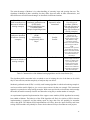
The main advantage of Mahout is its robust handling of extremely large and growing data sets. The
algorithms in Mahout all share scalability, but they differ from each other in other characteristics, and
these differences offer different advantages or drawbacks in different situations.
Size of data set
Small to medium (less
than tens of millions of
training examples)
Mahout algorithm
Stochastic gradient descent
(SGD) family:
OnlineLogisticRegression,
CrossFoldLearner,
AdaptiveLogisticRegression
Executive model
Sequential, online.
incremental
Characteristics
Uses all types of
predictor variables;
sleek and efficient over
the appropriate data
range (up to millions of
training examples)
Medium to large
(millions to hundreds
of millions of training
examples)
Support Vector Machine
(SVM)
Naïve Bayes
Complementary Naïve
Bayes
Sequential
Small to medium (less
than tens of millions of
training examples)
Random forests
Parallel
Experimental still: sleek and
efficient over the
appropriate data range
Strongly prefers text-like
data; medium to high
overhead for training;
effective and useful for data
sets too large for SGD or
SVM
Somewhat more expensive
to train than naïve Bayes;
effective and useful for data
sets too large for SGD, but
has similar limitations to
naïve Bayes
Uses all types of predictor
variables; high overhead for
training; not widely used
(yet); costly but offers
complex and interesting
classifications, handles
nonlinear and conditional
relationships in data better
than other techniques
Parallel
Parallel
Table 2: Characteristics of the Mahout learning algorithms used for classification [16]
The algorithms differ somewhat in the overhead or cost of training, the size of the data set for which
they’re most efficient, and the complexity of analyses they can deliver.
Stochastic gradient descent (SGD) is a widely used learning algorithm in which each training example is
used to tweak the model slightly to give a more correct answer for that one example. This incremental
approach is repeated over many training examples. With some special tricks to decide how much to nudge
the model, the model accurately classifies new data after seeing only a modest number of examples.
An experimental sequential implementation of the support vector machine (SVM) algorithm has recently
been added to Mahout. The behavior of the SVM algorithm will likely be similar to SGD in that the
implementation is sequential, and the training speed for large data sizes will probably be somewhat
slower than SGD. The Mahout SVM implementation will likely share the input flexibility and linear
scaling of SGD and thus will probably be a better choice than naive Bayes for moderate-scale projects.
17
The naive Bayes and complementary naive Bayes algorithms in Mahout are parallelized algorithms that
can be applied to larger datasets than are practical with SGD-based algorithms. Because they can work
effectively on multiple machines at once, these algorithms will scale to much larger training data sets than
will the SGD-based algorithms.
The Mahout implementation of naive Bayes, however, is restricted to classification based on a single textlike variable. For many problems, including typical large data problems, this requirement isn’t a problem.
But if continuous variables are needed and they can’t be quantized into word-like objects that could be
lumped in with other text data, it may not be possible to use the naive Bayes family of algorithms.
In addition, if the data has more than one categorical word-like or text-like variable, it’s possible to
concatenate your variables together, disambiguating them by prefixing them in an unambiguous way.
This approach may lose important distinctions because the statistics of all the words and categories get
lumped together. Most text classification problems, however, should work well with naive Bayes or
complementary naive Bayes.
Mahout has sequential and parallel implementations of the random forests algorithm as well. This
algorithm trains an enormous number of simple classifiers and uses a voting scheme to get a single result.
The Mahout parallel implementation trains the many classifiers in the model in parallel.
This approach has somewhat unusual scaling properties. Because each small classifier is trained on some
of the features of all of the training examples, the memory required on each node in the cluster will scale
roughly in proportion to the square root of the number of training examples. This isn’t quite as good as
naive Bayes, where memory requirements are proportional to the number of unique words seen and thus
are approximately proportional to the logarithm of the number of training examples. In return for this less
desirable scaling property, random forests models have more power when it comes to problems that are
difficult for logistic regression, SVM, or naive Bayes. Typically these problems require a model to use
variable interactions and discretization to handle threshold effects in continuous variables. Simpler
models can handle these effects with enough time and effort by developing variable transformations, but
random forests can often deal with these problems without that effort.
1.2 Classification Configuration
For classification of text, this primarily means encoding the features and then creating vectors out of the
features, but it also includes setting up training and test sets. The complete set of steps taken is:
(1) Convert the raw text files into Hadoop's SequenceFile format.
(2) Convert the SequenceFile entries into sparse vectors and modify the labels.
(3) Split the input into training and test sets:
bin/mahout split --input $SEQ2SPLABEL --trainingOutput $TRAIN --testOutput $TEST
--randomSelectionPct 20 --overwrite –sequenceFiles
(4) Run the naive Bayes classifier to train and test:
18
a. bin/mahout trainnb -i $TRAIN -o $MODEL -extractLabels --labelIndex $LABEL
b. bin/mahout testnb -i $TEST -m $MODEL --labelIndex $LABEL
The two main steps worth noting are Step (2) and Step (4). Step (2)a is the primary feature-selection and
encoding step, and a number of the input parameters control how the input text will be represented as
weights in the vectors.
Table 3: Options of Mahout feature vector generation [16]
The analysis process in Step (2)a is worth diving into a bit more, given that it is doing much of the heavy
lifting needed for feature selection. A Lucene Analyzer is made up of a Tokenizer class and zero or more
TokenFilter classes. The Tokenizer is responsible for breaking up the original input into zero or more
tokens (such as words). TokenFilter instances are chained together to then modify the tokens produced by
the Tokenizer. For example, the Analyzer used in the example:
<1> Tokenizes on whitespace, plus a few edge cases for punctuation.
<2> Lowercases all tokens.
<3> Converts non-ASCII characters to ASCII, where possible by converting diacritics and so on.
<4> Throws away tokens with more than 40 characters.
<5> Removes stop words.
<6> Stems the tokens using the Porter stemmer.
The end result of this analysis is a significantly smaller vector for each document, as well as one that has
removed common "noise" words (the, a, an, and the like) that will confuse the classifier. This Analyzer
was developed iteratively by looking at examples and then processing it through the Analyzer and
examining the output, making judgment calls about how best to proceed.
19
Step (2)b does some minor conversions of the data for processing as well as discards some content so that
the various labels are evenly represented in the training data.
Step (4) is where the actual work is done both to build a model and then to test whether it is valid or not.
In Step (4)a, the --extractLabelsoption simply tells Mahout to figure out the training labels from the input.
(The alternative is to pass them in.) The output from this step is a file that can be read via the
org.apache.mahout.classifier.naivebayes.NaiveBayesModel class. Step (4)b takes in the model as well as
the test data and checks to see how good of a job the training did.
2. Environment Setup
2.1 Installation
Install Solr:
Installation progress:
1: Download the Java SE 7 JDK and export environment variables. Check “java -version”.
2: Download the Apache Ant binary distribution (1.9.4) from http://ant.apache.org/ and export
environment variable ANT_HOME. Use “ant -version” to check.
3: Download the Apache Solr distribution (Source code) and extract to C:\solr\
4: Navigate to the Solr directory and use “ant compile” to compile Solr. (Use the ant ‘ ivy-bootstrap’
command to install ivy.jar before installing Solr)
5: Successfully installed Solr.
Or you can directly download the binary version of Solr and then launch Solr.
A screenshot of the Solr client webpage is shown in Figure 1.
20
Fig. 1: Solr Installation
Install Cloudera virtualbox VM:
1. Download latest version of Virtualbox and install.
2. Download cloudera-quickstart-vm-5.3.x.zip and then unzip to your virtualbox machine folder.
3. Run virtualbox and run “import applicance” in the File menu.
4. Find your Cloudera unzipped file and click open.
5. Click “Continue”.
6. Click “import”
7. Click “Continue”
8. Successfully import the virtualbox.
21
Fig. 2: Cloudera Virtual Machine Installation
9. Click “start” to start the virtual machine OS.
Install Mahout:
Prerequisites:
1. Java JDK 1.8
2. Apache Maven
Checkout the sources from the Mahout GitHub repository either via
git clone https://github.com/apache/mahout.git
Compiling
Compile Mahout using standard maven commands
mvn clean compile
2.2 Data Import
2.2.1 Approach
We renamed the test data CSV file to books.csv, put it at example/exampledocs/books.csv and uploaded it
to the Solr example server.
We used HTTP-POST to send the CSV data over the network to the Solr server:
cd example/exampledocs
curl http://localhost:8983/solr/update/csv --data-binary @books.csv -H 'Content-type:text/plain;
22
charset=utf-8'
2.2.2 Steps
a. Modify the data CSV file
We added a row describing each column at the beginning of the data CSV file.
Figure 3 shows what we have added to the existing data CSV file:
Fig. 3: Data CSV file modification example
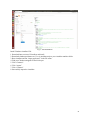
b. Change schema.xml to define properties of the fields.
The schema declares what kinds of fields there are, which field should be used as the unique/primary key,
which fields are required and how to index and search each field. For each new field, we add name, type,
indexed and stored attribute. Name is mandatory and it is the name for the field. Type is mandatory and it
is the name of a previously defined type from the <types> section. Indexed is set to true if this field
should be indexed. Stored is set to true if this field should be retrievable.
Figure 4 shows what we have added to the existing schema.xml:
Fig. 4: Schema.xml modification example
c. Upload the CSV
d. Restart Solr
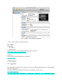
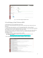
2.2.3 Results
We conducted a query without any keyword and the result was captured as shown in Figure 5, which
shows we have successfully imported books.csv to Solr:
23
Fig. 5: Import CSV file to Solr
2.3 Upload Tweets and Webpages of Small Collection to Solr
a. Download our small collection. We use the accident data (z356t.csv) as our small collection.
b. Download the script from TA. We use the tweet_URL_archivingFile.py to deal with our z356.csv file.
It extracts the URL of all the tweets. Then it calculates the frequency of each URL and then gives out a
sorted result for the URL with its frequency in the file shortURLs_z356.txt. At this time, we can set a
threshold and takes the URLs whose frequency is higher than the threshold. The
tweet_URL_archivingFile.py will translate URLs in abbreviation version to their complete version. Then
it will output a translation form, which includes the full version URLs with its corresponding abbreviation
version in file short_origURLsMapping_z356.txt. Also, the script will download the real webpage of
these URLs and save it as *.txt file.
c. We can see that from our threshold, we can only get 12 webpages. They totally appear 952 times.
d. We tried to upload the tweets with webpages to Solr. We discussed with our TA about how to upload
them to Solr.
We think about 2 approaches:
1) Use the post.jar. But we still have to do preprocessing to merge the webpages and tweets.
2) Write our own script using Python/Java/C to do the preprocessing and then use an API library to
connect to Solr inside the script and then upload our results to Solr.
24
We finally choose the second method to finish this job since we tried many times and still could not
figure out how to successfully use the post.jar to upload the webpages and tweets at the same time.
e. We choose the solrpy library to connect to Solr inside the script and then use the script to preprocess
the script and upload to Solr.
f. We first tested the solrpy library. This is the test code from the solrpy website.
# create a connection to a Solr server
s = solr.SolrConnection('http://example.org:8083/solr')
# add a document to the index
doc = dict(
id=1,
title='Lucene in Action',
author=['Erik Hatcher', 'Otis Gospodneti'],
)
s.add(doc, commit=True)
Here we came across a problem. This example does not work for our Solr. Finally we searched the
internet and found that we should use s.add(_commit=True,**doc) instead of s.add(doc, commit=True).
The key of the dic structure should be included in the schema of Solr.
g. Then we do the preprocessing for the metadata.
To be short, we need to read all the tweets in the z356.csv. For each tweet, we should extract the URL.
Next, check if the URLs are selected because of their high frequency. Then we form a dictionary structure,
which includes the ID, date, and its corresponding webpages as content. At last we upload the dictionary
structure to Solr. This below is the code with annotation.
import solr
# create a connection to a Solr server
psolr = solr.SolrConnection('http://localhost:8983/solr')
# connect with Solr
f=open('z356t.csv',"rb")
text = [line.decode('utf-8').strip() for line in f.readlines()]
f.close ( )
pid=[]
pdate=[]
pcontent=[]
pwebpage=[]
pname=[]
for row in text:
t=row.split("\t")
pcontent.append(t[0])
pname.append(t[1])
25
pid.append(t[2])
pdate.append(t[3])
#read the tweets
f=open('short_origURLsMapping_z356t.txt',"rb")
text = [line.decode('utf-8').strip() for line in f.readlines()]
f.close ( )
maap=dict([])
i=1;
for row in text:
t=row.split("--") #split the full version URL and its corresponding abbreviation version
q=t[1].split(",")
for o in q:
maap[o]=i
i=i+1
page=[]
page.append("blank")
for j in range(1,13):
s=str(j)+".txt"
f=open(s,"rb")
page.append(f.read().decode('utf-8').strip())
f.close()
# read webpage
for i in range(0,len(pid)):
t=-1
print i
for j in maap.keys():
if pcontent[i].find(j)>-1:
t=maap[j] #Find the corresponding webpage number.
if t==9:
t=8
if t>-1:
print "upload"+str(t)
upload=dict([])
upload["id"]=pid[i]
upload["mcbcontent"]=page[t]
upload["mcbposttime"]=pdate[i]
psolr.add(_commit=True,**upload)
#upload to Solr
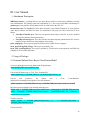
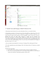
h. Figure 6 shows that we have successfully uploaded the tweets and their corresponding webpages to
Solr.
26
.
Fig. 6: Tweets and webpages uploaded to Solr
2.4 Load Webpages of Small Collection to HDFS
a. Download the new CSV file and Python script from TA
Hint: use pip to install Beautifuloap4 and requests which are used in the script. Otherwise the script
cannot run.
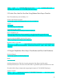
b. Use the script to deal with the new csv file. The generated long URLs is shown in Figure 7.
c. Install Nutch (follow the Nutch tutorial provided by TA). Because we do not need Nutch to upload the
new webpages to Solr, we need to modify the crawl script in Nutch.
d. We comment the code after “# note that the link inversion - indexing routine can be done within the
main loop # on a per segment basis” until the end of the script in order to prevent this code from
uploading data to Solr.
e. Use Nutch to crawl the webpages and upload them to HDFS:
 We put the URL seed we got from the script and save them to the directory “urls”.
 We run the command:
bin/crawl urls testcrawl/ TestCrawl/ http://localhost:8983/solr/ 1
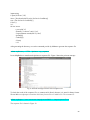
The screenshot after Nutch finished crawling the webpages is shown in Figure 8.
27
Fig. 7: LongURLs from the new tweets
Fig. 8: Nutch finished crawling the webpages
f. After we get the webpages data from Nutch, we uploaded it to HDFS for reducing noise team. We put
them under the directory /user/cs5604s15_class/pages/.
3. Naï
ve Bayes Classification
3.1 Transform Tweets to Sequence File and Feature Vector on Our Own Machine
In this section, we use Python and Mahout to transform our small collection CSV file to sequence file and
vectors. So we can use the command line of Mahout to get the word count and tf-idf vector file for our
small collection.
Mahout has utilities to generate vectors from a directory of text documents. Before creating the vectors,
we first convert the documents to SequenceFile format. Sequence File is a Hadoop class which allows us
to write arbitrary (key, value) pairs into it. The document vectorizer requires the key to be a text with a
unique document ID, and value to be the text content in UTF-8 format.
After searching online, we still cannot figure out an approach to generate the CSV format tweet to
sequence file. The only solution is what we found on the VTTECHWORK
(https://vtechworks.lib.vt.edu/bitstream/handle/10919/47945/Mahout_Tutorial.pdf?sequence=11).
In order to transform the CSV format tweet to sequence file, we developed another way. We first use
Python to read the CSV file and store each row into a separate text file with its row number being the file
name. We put these text files into one directory.
The Python code is like this:
28
import string
f=open('z356t.csv',"rb")
#text = [line.decode('utf-8').strip() for line in f.readlines()]
text = [line for line in f.readlines()]
f.close ( )
i=0;
for row in text:
t=row.split("\t")
filename="./rawtext/"+str(i)+".txt"
f=open(filename.encode('utf-8'),"wbr")
#print(t[0])
f.write(t[0])
f.close()
i=i+1
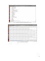
After generating the directory, we use the command provide by Mahout to generate the sequence file.
mahout seqdirectory -c UTF-8 -i plaintext/ -o pt_sequences/
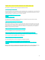
It uses MapReduce to transform the plaintext to sequence file. Figure 9 shows the print out message.
Fig. 9: Print out message from text file to sequence file
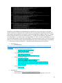
To check the result of the sequence file, we cannot read it directly because it is stored in binary format.
We use Mahout seqdumper to transform this binary format file to a readable file. The command is:
mahout seqdumper -i /user/<user-name>/output/part-m-00000 -o ~/output/sequencefile.txt
The sequence file is shown in Figure 10.
29
Fig. 10: Generated sequence file
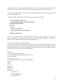
From the result, we can see that we are on the right track. The key is the file name, which is the row
number of the tweets and the values are the content of the tweets.
After that we try to create the vector file, which needs the word count and tf-idf. We also use the abovementioned commend to transform the binary vector file to readable file.
This will take any plain text files in the directory “inputdirectory” and convert them to sequence files.
We specify the UTF8 character set to make sure each file inside the input directory is processed using the
same set rather than being able to specify individual character sets. These sequence files must next be
converted to vector files that Mahout can then run any number of algorithms on. To create these vector
files, you will need to run the command:
mahout seq2sparse -i sequences -o outputdirectory –ow –chunk 100 –x 90 –seq –ml 50 –n 2 -nv
The ‘-nv’ flag means that we use named vectors, so that the data files will be easier to inspect by hand.
The ‘-x 90’ flag means that any word that appears in more than 90% of the files is a stop word, or a word
is too common and thus is filtered out (i.e. articles such as ‘the’, ‘an’, ‘a’, etc.).
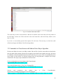
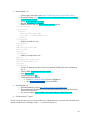
Figure 11 shows the print out message when we have successfully generated the vectors. Figure 12 shows
the generated tf-idf results while Figure 13 shows the generated word count results.
30
Fig. 11: Print out message from sequence file to vectors
Fig. 12: Generated tf-idf results
31
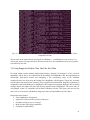
Fig. 13: Generate word count results
The reason why we show word count here is that the row number of the word is that of the key number in
the tf-idf table. So there are 5999 words here in the word count table, and the tf-idf key number varies
from 1 to 5999.
Up to now, we successfully generate the sequence file and vector. The next step is to label the small
collection and apply the Mahout Classification algorithms.
3.2 Commands for Classification with Mahout Naï
ve Bayes Algorithm
We have two folders for tweets: one folder contains 100 text files of positive tweets that are related to the
topic; the other folder contains 100 text files of negative tweets that are not related to the topic. All tweets
are randomly selected using Python from the small collection we are given. Then we uploaded the tweets
to the cluster. On the cluster, we followed example from [2] and performed a complete Naïve Bayes
classification. The step-by-step commands are listed as below.
Create a working directory for the dataset and all input/output:
export WORK_DIR=/user/cs5604s15_class/
Convert the full dataset into a <Text, Text> SequenceFile:
mahout seqdirectory -i ${WORK_DIR}/test -o ${WORK_DIR}/test-seq -ow
Convert
and
preprocess
the
dataset
into
a
<Text,
VectorWritable>
SequenceFile containing term frequencies for each document:
mahout seq2sparse -i ${WORK_DIR}/test-seq -o ${WORK_DIR}/test-vectors -lnorm -nv -wt tfidf
32
Split the preprocessed dataset into training and testing sets:
mahout split -i ${WORK_DIR}/test-vectors/tfidf-vectors --trainingOutput ${WORK_DIR}/test-trainvectors --testOutput ${WORK_DIR}/test-test-vectors
--randomSelectionPct 40 --overwrite -sequenceFiles -xm sequential
Train the classifier:
mahout trainnb -i ${WORK_DIR}/test-train-vectors
${WORK_DIR}/labelindex -ow -c
-el
-o
Test the classfier:
mahout
testnb
-i
${WORK_DIR}/test-test-vectors
-m
${WORK_DIR}/labelindex -ow -o ${WORK_DIR}/test-testing –c
${WORK_DIR}/model
-li
${WORK_DIR}/model
-l
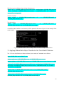
A confusion matrix and the overall accuracy will be printed on the screen. Figure 14 is an example of the
sample output.
Fig. 14: Confusion Matrix and Accuracy Statistics from Naïve Bayes classification
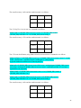
3.3 Applying Mahout Naïve Bayes Classifier for Our Tweet Small Collection
Test 1: Tweets classification, no feature selection, test on train set. Commands are as follows:
export WORK_DIR=/user/cs5604s15_class
mahout seqdirectory -i ${WORK_DIR}/tweets -o ${WORK_DIR}/tweets-seq -ow
mahout seq2sparse -i ${WORK_DIR}/tweets-seq -o ${WORK_DIR}/tweets-vectors -lnorm -nv -wt tfidf
mahout split -i ${WORK_DIR}/tweets-vectors/tfidf-vectors --trainingOutput ${WORK_DIR}/tweetstrain-vectors --testOutput ${WORK_DIR}/tweets-test-vectors --randomSelectionPct 20 --overwrite -sequenceFiles -xm sequential
mahout trainnb -i ${WORK_DIR}/tweets-train-vectors -el -o ${WORK_DIR}/model -li
${WORK_DIR}/labelindex -ow -c
mahout testnb -i ${WORK_DIR}/tweets-train-vectors -m ${WORK_DIR}/model -l
${WORK_DIR}/labelindex -ow -o ${WORK_DIR}/tweets-testing -c
33
The overall accuracy is 96% and the confusion matrix is as follows:
Positive
Negative
Positive
86
3
Negative
4
95
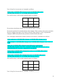
Test 2: Using Test 1, test on test set. Command is as follows:
mahout testnb -i ${WORK_DIR}/tweets-test-vectors -m ${WORK_DIR}/model -l
${WORK_DIR}/labelindex -ow -o ${WORK_DIR}/tweets-testing –c
The overall accuracy is 70% and the confusion matrix is as follows:
Positive
Negative
Positive
7
3
Negative
0
0
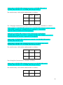
Test 3: Tweets classification, using feature selection, test on train set. Commands are as follows:
mahout seq2sparse -i ${WORK_DIR}/tweets-seq -o ${WORK_DIR}/tweets-vectors --norm 2 --weight
TFIDF --namedVector --maxDFPercent 90 --minSupport 2 --analyzerName
org.apache.mahout.text.MailArchivesClusteringAnalyzer
mahout split -i ${WORK_DIR}/tweets-vectors/tfidf-vectors --trainingOutput ${WORK_DIR}/tweetstrain-vectors --testOutput ${WORK_DIR}/tweets-test-vectors --randomSelectionPct 20 --overwrite -sequenceFiles -xm sequential
mahout trainnb -i ${WORK_DIR}/tweets-train-vectors -el -o ${WORK_DIR}/model -li
${WORK_DIR}/labelindex -ow -c
mahout testnb -i ${WORK_DIR}/tweets-train-vectors -m ${WORK_DIR}/model -l
${WORK_DIR}/labelindex -ow -o ${WORK_DIR}/tweets-testing -c
The overall accuracy is 99% and the confusion matrix is as follows:
Positive
Negative
Positive
78
1
Negative
1
98
34
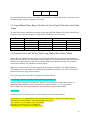
Test 4: Using Test 3, test on test set. Command is as follows:
mahout testnb -i ${WORK_DIR}/tweets-test-vectors -m ${WORK_DIR}/model -l
${WORK_DIR}/labelindex -ow -o ${WORK_DIR}/tweets-testing –c
The overall accuracy is 100% and the confusion matrix is as follows:
Positive
Negative
Positive
18
0
Negative
0
0
We can observe that feature selection for tweets can help improve accuracy.
We use the script from TA to download some of the webpages. Then we choose some positive (related to
the topic) webpages and negative (not related to the topic) pages manually. At last, we upload these
webpages to HDFS and repeat the same procedure as what we did for the tweets.
Test 5: Webpages classification, no feature selection, test on train set. Commands are as follows:
mahout seqdirectory -i ${WORK_DIR}/webpages -o ${WORK_DIR}/webpages-seq -ow
mahout seq2sparse -i ${WORK_DIR}/webpages-seq -o ${WORK_DIR}/webpages-vectors -lnorm -nv wt tfidf
mahout split -i ${WORK_DIR}/webpages-vectors/tfidf-vectors --trainingOutput
${WORK_DIR}/webpages-train-vectors --testOutput ${WORK_DIR}/webpages-test-vectors -randomSelectionPct 20 --overwrite --sequenceFiles -xm sequential
mahout trainnb -i ${WORK_DIR}/webpages-train-vectors -el -o ${WORK_DIR}/model -li
${WORK_DIR}/labelindex -ow -c
mahout testnb -i ${WORK_DIR}/webpages-train-vectors -m ${WORK_DIR}/model -l
${WORK_DIR}/labelindex -ow -o ${WORK_DIR}/webpages-testing –c
The overall accuracy is 100% and the confusion matrix is as follows:
Positive
Negative
Positive
55
0
Negative
0
28
Test 6: Using Test 5, test on test set. Command is as follows:
35
mahout testnb -i ${WORK_DIR}/webpages-test-vectors -m ${WORK_DIR}/model -l
${WORK_DIR}/labelindex -ow -o ${WORK_DIR}/webpages-testing –c
The overall accuracy is 94% and the confusion matrix is as follows:
Positive
Negative
Positive
14
0
Negative
1
2
Test 7: Webpages classification, using feature selection, test on train set. Commands are as follows:
mahout seq2sparse -i ${WORK_DIR}/webpages-seq -o ${WORK_DIR}/webpages-vectors-fs --norm 2 -weight TFIDF --namedVector --maxDFPercent 90 --minSupport 2 --analyzerName
org.apache.mahout.text.MailArchivesClusteringAnalyzer
mahout split -i ${WORK_DIR}/webpages-vectors-fs/tfidf-vectors --trainingOutput
${WORK_DIR}/webpages-train-vectors-fs --testOutput ${WORK_DIR}/webpages-test-vectors-fs -randomSelectionPct 20 --overwrite --sequenceFiles -xm sequential
mahout trainnb -i ${WORK_DIR}/webpages-train-vectors-fs -el -o ${WORK_DIR}/model -li
${WORK_DIR}/labelindex -ow -c
mahout testnb -i ${WORK_DIR}/webpages-train-vectors-fs -m ${WORK_DIR}/model -l
${WORK_DIR}/labelindex -ow -o ${WORK_DIR}/webpages-testing –c
The overall accuracy is 84% and the confusion matrix is as follows:
Positive
Negative
Positive
58
0
Negative
13
12
Test 8: Using Test 7, test on test set. Command is as follows:
mahout testnb -i ${WORK_DIR}/webpages-test-vectors-fs -m ${WORK_DIR}/model -l
${WORK_DIR}/labelindex -ow -o ${WORK_DIR}/webpages-testing –c
The overall accuracy is 65% and the confusion matrix is as follows:
Positive
Positive
Negative
11
0
36
Negative
6
0
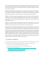
We concluded that the accuracy of webpage is not good here is mainly due to that we did not use the
cleaned webpages. Original webpages is very noisy.
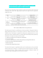
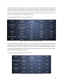
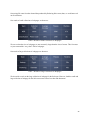
3.4 Using Mahout Naïve Bayes Classifier for Tweet Small Collections from Other
Teams
We used the training tweet datasets from other groups and applied the Mahout Naive Bayes classification
algorithm. If the results are not good, we apply feature selection to revise our model.
Team
LDA
Hadoop
NER
Reducing Noise
No Feature Selection
Test on Train Set
Test on Test set
99%
95%
95%
76%
100%
100%
99%
93%
Feature Selection
Test on Train Set
Test on Test Set
99%
81%
3.5 Generate Class Label for New Data Using Mahout Naï
ve Bayes Model
We are able to use Mahout to train and test our classification model. However, the test data provided to
Mahout has to be labeled. The next problem is how to apply the classification model to new unlabeled test
data. However, Mahout does not provide any function to label new unlabeled test data. The generated
classification model given by Mahout is in binary format.
Right now we find an article [17] about applying the Naive Bayes classifier to new unlabeled datasets.
This method is also recommended in “Learning Apache Mahout Classification” [20]. We tried to follow
the tutorial and try to apply the new classifier.
First of all, we get the scripts and Java programs used in the tutorials.
git clone https://github.com/fredang/mahout-naive-bayes-example.git
Then we want to compile the Java programs. However, our system does not have Maven. Thus, we
downloaded and installed the latest version of Maven, which is Maven 3.3.1. We exported the
JAVA_HOME. We can use this command to check if Maven is successfully installed.
mvn –version
Messages we get are as follows and we can see that Maven is successfully installed.
Apache Maven 3.3.1 (cab6659f9874fa96462afef40fcf6bc033d58c1c; 2015-03-13T16:10:27-04:00)
Maven home: /home/cs5604s15_class/maven/apache-maven-3.3.1
Java version: 1.7.0_55, vendor: Oracle Corporation
Java home: /usr/java/jdk1.7.0_55-cloudera/jre
Default locale: en_US, platform encoding: UTF-8
37
OS name: "linux", version: "2.6.32-504.8.1.el6.x86_64", arch: "amd64", family: "unix"
We continue to compile the code by running the command as follows.
mvn clean package assembly:single
We got some JAR files in the target directory after running the above command and we can use these files
to generate labels for new data sets. To repeat the same procedure as described in the tutorial, we tried to
use the same dataset. To get the tweets, we use these command:
git clone https://github.com/tweepy/tweepy.git
cd tweepy
sudo python setup.py install
We change the file script/twitter_fetcher.py with our new consumer keys/secrets and access token
key/secrets to use the API to download tweets.
python scripts/twitter_fetcher.py 5 > tweets-train.tsv
The tweet files contains a list of tweets in a tab separated value format. The first number is the tweet ID
followed by the tweet message, which is identical to our previous format. We want to use this method to
generate labels for new tweets. We have the tweet-to-classify.tsv in our data directory. We upload it to
HDFS by using the following command:
hadoop fs -put data/tweets-to-classify.tsv tweets-to-classify.tsv
We run the MapReduce job by using the following command:
hadoop jar target/mahout-naive-bayes-example2-1.0-jar-with-dependencies.jar model tweetsvectors/dictionary.file-0 tweets-vectors/df-count/part-r-00000 tweets-to-classify.tsv tweet-category
We can copy the results from HDFS to the local filesystem:
hadoop fs -getmerge tweet-category tweet-category.tsv
Our result should be able to read by a filereader by running the command:
java -cp target/mahout-naive-bayes-example2-1.0-jar-with-dependencies.jar
com.chimpler.example.bayes2.ResultReader data/tweets-to-classify.tsv [label index path] tweetcategory.tsv
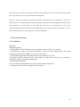
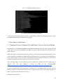
However, on our cluster, we come across the error shown in Figure 15. We are still working on this issue.
We hope that we can generate labels for new unlabeled test tweets when we solve this problem.
38
Fig. 15: Error message when generating classification labels for new unlabeled test data
We discussed with Mohamed and Sunshin about our problem. We also tried to come up with other
possible solutions for classification label prediction, such as using Python and Hadoop streaming API,
using Apache Spark and MLlib, or using other classification algorithms in Mahout. However, we found
the only difference between our trial and the tutorial [17] was the version of Hadoop. The tutorial [17]
was using Hadoop 1.1.1 and our cluster was using Hadoop 2.5. Thus, we tried to install Hadoop 1.1.1 on
our own machine and this actually solved the problem. Our current progress is that we are able to predict
labels for new unlabeled test data using trained Mahout Naïve Bayes classification model using Hadoop
1.1.1. We state our efforts on Hadoop 1.1.1 installation and label prediction result as follows.

Install Java 1.6
o Download from
http://www.oracle.com/technetwork/java/javaee/downloads/java-ee-sdk-6u3-jdk-6u29-downloads523388.html
o Uncompress jdk-6u35-linux-x86-64.bin
 chmod u+x jdk-6u35-linux-x64.bin
 ./jdk-6u35-linux-x64.bin
o Copy the directory jdk-1.6.035 to /usr/lib
 sudo mkdir -p /usr/lib/jvm
 sudo cp -r jdk1.6.0_35 /usr/lib/jvm/jdk1.6.0_35
o Setup environment variable
 sudo gedit /etc/profile
 export JAVA_HOME=/usr/lib/jvm/jdk1.6.0_35
 export JRE_HOME=${JAVA_HOME}/jre
 export CLASSPATH=.:${JAVA_HOME}/lib:${JRE_HOME}/lib
 export PATH=${JAVA_HOME}/bin:${JRE_HOME}/bin:$PATH
 source /etc/profile
o Test installation of Java
 java –version

Install Maven
o Download from: https://maven.apache.org/download.cgi
o Since version 3.3.1 is not compatible with Java 1.6, we changed to version 3.2.1
39

Install Hadoop 1.1.1
o
o
Following the instructions from: http://6341986.blog.51cto.com/6331986/1143596
Download Hadoop 1.1.1: wget http://mirror.bit.edu.cn/apache/hadoop/common/hadoop1.1.1/hadoop-1.1.1.tar.gz
o Unzip: tar zxvf hadoop-1.1.1.tar.gz
o Rename: mv hadoop-1.1.0 hadoop
o Modify conf/core-site.xml: gedit conf/core-site.xml and add:
conf/core-site.xml:
<configuration>
<property>
<name>fs.default.name</name>
<value>hdfs://localhost:9000</value>
</property>
</configuration>
o Modify conf/hdfs-site.xml:
<configuration>
<property>
<name>dfs.replication</name>
<value>1</value>
</property>
</configuration>
o Modify conf/mapred-site.xml:
<property>
<name>mapred.job.tracker</name>
<value>localhost:9001</value>
</property>
</configuration>
o In order for Hadoop to be able to find Java, add path of JDK at the end of conf/hadoopenv.sh
o Format HDFS: bin/hadoop namenode -format
o Start: bin/start-all.sh
o Check start progress: jps
o Check installation of Hadoop
 Open http://localhost:50030 for status of MapReduce
 Open http://localhost:50070 for status of HDFS

Install Mahout 0.8
o Download Mahout 0.8 from https://archive.apache.org/dist/mahout/0.8/
o Download mahout-distribution-0.8.tar.gz and mahout-distribution-0.8.pom and convert
this pom file to pom.xml
o Use mvn to compile: mvn clean && mvn compile && mvn -DskipTests install

Follow tutorial [17] again
We can see for each tweet, we give the tweet ID, tweet content and its score for each class and final result
in terms of which class it belongs to (with “=>”) as shown in Figure 16.
40
Fig. 16: Using Mahout Classification Model and Additional Program to Predict Class Labels of New
Unlabeled Test Data
We can work on the small collections using our own Hadoop 1.1.1 and Mahout 0.8 now; however, we
will run out of space for large collections. We then moved on for new method that can be used to predict
class labels for new data.
3.5 Using Pangool to Predict Class Label for New Data
We found another Apache Hadoop implementation library, Pangool [19]. Pangool is a Java, low-level
MapReduce API. It aims to be a replacement for the Hadoop Java MapReduce API. By implementing an
intermediate Tuple-based schema and configuring a Job conveniently, many of the accidental
complexities that arise from using the Hadoop Java MapReduce API disappear. Things like secondary
sort and reduce-side joins become extremely easy to implement and understand. Pangool's performance is
comparable to that of the Hadoop Java MapReduce API. Pangool also augments Hadoop's API by making
multiple outputs and inputs first-class and allowing instance-based configuration. The reason why we
used Pangool is that it is compatible with all kinds of Hadoop versions. This library does not have the
same issue we come across with Mahout. Pangool provides an implementation of Naïve Bayes.
Pangool has some features:
 Easier MapReduce development.
 Support for Tuples instead of just Key/Value pairs.
 Secondary sorting as easy as it can get.
 Built-in reduce-side joining capabilities.
 Performance and flexibility.
41




Configuration by object instance instead of classes.
First-class multiple inputs & outputs.
Built-in serialization support for Thrift and ProtoStuff.
100% Hadoop compatibility. 0.20.X, 1.X, 2.X and YARN.
We download Pangool using: git clone https://github.com/datasalt/pangool.git. To install Pangool, we
should use maven. The version we used here is maven 3.3.1, and the Java version we used is 1.7.0_55.
After installation of maven, we just simple use this command: mvn clean install.
The
Naïve
Bayes
implementation
is
under
pangool/examples/src/main/java/com/datasalt/pangool/examples/naivebayes/.
the
directory
It has two classes:
NaiveBayesGenerate.java: This class is used to generate the Naïve Bayes classifier model.
NaiveBayesClassifier.java: This class will use the model we generated to predict and label the new data.
We used the Naïve Bayes example under target/pangool-examples-0.71-SNAPSHOT-hadoop.jar
Now we will give an example of the classification process.
First, we will label our data to generate the training set. For tweets, we will add a POSITIVE before the
tweets that are related to this topic. We will add a NEGATIVE before the tweets that are not related to
this topic. The label and the content of tweet are separated by a TAB. An example of the training set is as
shown in Figure 17.
42
Fig. 17: Example of Training Set
When we are done with labeling, we use the NaïveBayesGenerate.java class to generate the model. The
command is as follows:
hadoop
jar
target/pangool-examples-0.71-SNAPSHOT-hadoop.jar
LDA/train_lda.txt lda-out-bayes-model
naive_bayes_generate
The naive_bayes_generate is the class from Pangool. The LDA/train_lda.txt is the training data we
showed in Figure . The lda-out-bayes-model is the Naï
ve Bayes model we generated.
Then we used the labeled data to test the accuracy of our classifier. We split the labeled data into train set
and test set (80% and 20%). The train set was used in last step. The test set was used without the label.
We used the model and the NaiveBayesClassifier.java class to classify the testing data. We compared the
manually assigned label and the predicted label and calculated the accuracy. The command is shown as:
hadoop jar target/pangool-examples-0.71-SNAPSHOT-hadoop.jar naive_bayes_classifier lda-out-bayesmodel/p* LDA/test_lda.txt out-classify-lda
We used the naïve_bayes_clasifier class with our model lda-out-bayes-model/p* to apply classification
for the LDA/test_lda.txt and outputed the labeled data, out-classify-lda. We conducted 5-fold cross
validation to make sure that our model works fine for this text classification task. We will show our
summary of accuracy in Section IV.4.
We used this classifier to classify new data (small tweets, small webpages, large tweets and large
webpages).
However, the input file and output file we used and generated are plain text. However, we need to read
cleaned data from Reducing Noise team, which is in AVRO format. We should also have our output file
in AVRO format in order for Hadoop team to upload to HBase. We give our thanks to Jose Cadena from
Hadoop team. He helped us to modify the code and finally we can read in the AVRO file and generate the
AVRO file with the correct schema. The command for labeling new data is shown as:
hadoop
jar
mr-naivebayes.jar
lda-out-bayes-model/p*
43
/user/cs5604s15_noise/TWEETS_CLEAN/suicide_bomb_attack_S
classified_tweets_LDA_afghanistan_small
We used our new JAR file to classify the new data, which has already been cleaned by Reducing Noise
team and generated the AVRO file that could be uploaded to HBase. In this project, we have other teams
to label their own small collection of tweets. For small webpages, large tweets, and large webpages, we
manually labeled some of the topics to compare the performance.
4. Evaluation
4.1 Cross Validation
Learning the parameters of a prediction function and testing it on the same data is a methodological
mistake: a model that would just repeat the labels of the samples that it has just seen would have a perfect
score but would fail to predict anything useful on yet-unseen data. This situation is called overfitting. To
avoid it, it is common practice when performing a supervised machine learning experiment to hold out
part of the available data as a test set. However, by partitioning the available data into sets, we drastically
reduce the number of samples which can be used for learning the model, and the results can depend on a
particular random choice for the pair of (train, validation) sets. A solution to this problem is a procedure
called cross-validation (CV for short). A test set should still be held out for final evaluation, but the
validation set is no longer needed when doing CV. In the basic approach, called k-fold CV, the training
set is split into k smaller sets (other approaches are described below, but generally follow the same
principles). The following procedure is followed for each of the k “folds”:
●
A model is trained using k – 1 of the folds as training data;
●
The resulting model is validated on the remaining part of the data (i.e., it is used as a test set
to compute a performance measure such as accuracy).
The performance measure reported by k-fold cross-validation is then the average of the values computed
in the loop. This approach can be computationally expensive, but does not waste too much data (as it is
the case when fixing an arbitrary test set), which is a major advantage in problems such as inverse
inference where the number of samples is very small.
KFold divides all the samples in k groups of samples, called folds of equal sizes. The prediction function
is learned using k – 1 folds, and the fold left out is used for testing.
4.2 Summary of Results
To summarize our classification results, we listed the collection we worked on, the average accuracy
44
among the 5-fold cross validation, the size of new file for prediction, and the runtime of prediction. We
can see that the accuracy is generally good. Although some of the new file is pretty large, the runtime is
still acceptable. We noticed that the runtime would not increase linearly with respect to the filesize. This
is because we found the number of mappers involved was different among the programs. Thus, for a
larger file, the program will use more computing resources.
Our results of small collections of tweets are shown as:
Table 4: Results of Small Collections of Tweets
Since the performance of Hadoop team’s collection, we looked into their data and found that the data
contains many Arabic words. We thought that’s the reason that causes the accuracy to not be good. We
found the accuracy of NER team’s data is 100%. We looked into their data and found that their negative
tweets are selected from other collections. We did no further work on their data since the trained classifier
would not be able to classify their collection.
Our results of large collections of tweets are shown as:
Table 5: Results of Large Collections of Tweets
45
Our testing file came from the cleaned data produced by Reducing Noise team; thus, we could not work
on all collections.
Our results of small collections of webpages are shown as:
Table 6: Results of Small Collections of Webpages
We can see that the sizes of webpages are not necessarily larger than the sizes of tweets. This is because
we just extracted the “text_clean” field of webpages.
Out results of large collections of webpages are shown as:
Table 7: Results of Large Collections of Webpages
We also tried to work on the large collection of webpage for the Solr team. However, both the small and
large collection of webpage for the Solr team seems to have less than 200 documents.
46
V. Timeline/Schedule
This table shows our schedule for this project.
Time
Work progress
Week 1
Literature Review
Week 2
Environment setup (JAVA, Solr, Python), data import (Solr).
Test Python library scikit-learn and preprocessing the data. (for single node testing)
Week 3
Environment setup (Cloudera, Hadoop, Mahout).
Test Mahout classification tool (Random Forest and Naive Bayes) for cluster
Draft final report
Week 4
Test creating vectors from text using mahout.
Week 5
1. Use TA’s script to play with the small collection.
2. Download the corresponding webpage for each tweet and process the URLs, then
select tweets with high frequency and then upload them to Solr.
3. Finish documenting the schema that describes the specific output our team will produce for
each of the web pages.
Week 6
Spring break
Week 7
Use Mahout to do feature selection for our example data (aircraft accident).
1.Converting directory of documents to SequenceFile format
2.Creating Vectors from SequenceFile
3.Creating Normalized TF-IDF Vectors from a directory of text documents
4.Converting existing vectors to Mahout's format
Week 8
1. Upload webpages to HDFS.
2. Further investigate into Mahout classification.
Week 9
1. Finished using Nutch to crawl webpages
2. Apply classification for tweets and webpages
3. Compare performance between without feature selection and with feature selection
Week 10
Apply classification on tweet datasets provided by LDA, RN, NER and Hadoop team
Week 11
Work on methods to generate classification labels for unlabeled test data
Work on methods to apply classification to help searching in Solr
Week 12
Able to predict classification labels for new unlabeled test data using Hadoop 1.1.1
Week 13
Produce classification model and label predictions for tweets and webpages, for both
small collections and large collections
Week 14
Submitting
47
VI. Conclusion
In this project, our task is to classify tweet and webpage collections into pre-defined classes in order to
help with Solr search engine. We reviewed existing techniques and attempted to apply Apache Mahout
Naïve Bayes classification algorithm at the beginning. Apache Mahout Naïve Bayes classification
algorithm was able to provide accurate classifiers, however, it cannot predict labels for new data using the
model. “Learning Apache Mahout Classification” [20] provided a solution package to predict class labels
for new data using the classifiers generated by Mahout. However, this package was only able to work on
Hadoop 1.1.1, and it was not compatible with our cluster, which is Hadoop 2.5. We finally decided to use
another MapReduce Naïve Bayes package, Pangool [19], which was able to generate Naïve Bayes
classifiers and predict class labels for new data. We finished prediction of small collections of tweets for
our team, LDA team, Reducing Noise team, Solr team, and Hadoop team. We finished prediction of large
collections of tweets for our team, LDA team, Reducing Noise team, and Hadoop team. We finished
prediction of small collections of webpages for our team and NER team. We finished prediction of large
collections of webpages for Hadoop team and Clustering team. The accuracy of our Naïve Bayes model
was validated using 5-fold cross validation. Overall, The accuracy is satisfactory but still can be improved,
and the running time for the predictions is reasonable.
48
VII. Future Work
For performance improvement, future researchers should consider using larger training sets. Currently
due to the time limit, we are only able to label one hundred positive samples and one hundred negative
samples for each collection to be used as training set. Future researchers can still work on developing a
new package to label new data with the model generated by Apache Mahout. Future researchers can also
work on modifying the prediction package provided in “Learning Apache Mahout Classification” [20] to
make it compatible with higher versions of Hadoop, not just only Hadoop 1.1.1. Additional work is
needed on the Pangool package [19] to build more accurate classifiers. Trying to use tf-idf values instead
of word count in the feature vector, and using more representative features in feature selection, also may
improve the accuracy.
VII. Acknowledgements
We would like to thank our instructor Dr. Edward A. Fox, who brought us into this interesting project.
We would like to thank our TAs, Mohamed Magdy and Sunshin Lee, for their continued support and
valuable suggestions throughout the project. We would also give special thanks to Jose Cadena from the
Hadoop team, who helped us with input and output formatting problems. Further, we thank the Reducing
Noise team, which provided cleaned tweets and webpages for us to work on. Finally, thanks go to the
support of NSF grant IIS - 1319578, III: Small: Integrated Digital Event Archiving and Library (IDEAL).
49
VIII. References
[1] Apache Mahout: Scalable machine learning for everyone.
https://www.ibm.com/developerworks/library/j-mahout-scaling/, accessed on 02/12/2015.
[2] Twenty Newsgroups Classification Example.
https://mahout.apache.org/users/classification/twenty-newsgroups.html, accessed on 02/12/2015.
[3] Creating vectors from text.
http://mahout.apache.org/users/basics/creating-vectors-from-text.html, accessed on 02/12/2015.
[4] Classifying with random forests.
http://mahout.apache.org/users/classification/partial-implementation.html, accessed on 02/12/2015.
[5] Mahout 1.0 Features by Engine.
http://mahout.apache.org/users/basics/algorithms.html, accessed on 02/12/2015.
[6] Yoon, S., Elhadad, N., & Bakken, S. (2013). A Practical Approach for Content Mining of Tweets.
American Journal of Preventive Medicine, 45(1), 122–129. doi:10.1016/j.amepre.2013.02.025
[7] Cheng, Z., Caverlee, J., & Lee, K. (2010, October). You are where you tweet: a content-based
approach to geo-locating twitter users. In Proceedings of the 19th ACM international conference on
Information and knowledge management (pp. 759-768). ACM.
[8] Naive Bayes.
http://scikit-learn.org/stable/modules/naive_bayes.html, accessed on 02/05/2015.
[9] Random Forest.
http://scikit-learn.org/stable/modules/ensemble.html#random-forests, accessed on 02/05/2015.
[10] Cross validation.
http://scikit-learn.org/stable/modules/cross_validation.html, accessed on 02/05/2015.
[11] Update CSV.
https://wiki.apache.org/solr/UpdateCSV, accessed on 02/05/2015.
[12] Write schema.xml.
http://www.solrtutorial.com/schema-xml.html, accessed on 02/05/2015.
[13] NLTK.
http://www.nltk.org/, accessed on 02/05/2015.
[14] scikit-learn.
http://scikit-learn.org/stable/, accessed on 02/05/2015.
[15] An introduction to Information Retrieval, written by Christopher D. Manning, Prabhakar Raghavan,
Hinrich Schutze.
[16] Mahout in Action, written by Sean Owen, Robin Anil, Ted Dunning, Ellen Friedman.
[17] Using the Mahout Naï
ve Bayes classifiers to automatically classify twitter messages.
https://chimpler.wordpress.com/2013/03/13/using-the-mahout-naive-bayes-classifier-to-automaticallyclassify-twitter-messages/, accessed on 04/19/2015.
[18] Integrating the Mahout Bayes classifier with Solr.
http://www.oracle.com/technetwork/community/join/member-discounts/523387, accessed on 04/19/2015.
[19] Pangool Package.
http://pangool.net/overview.html, accessed on 05/06/2015.
[20] Learning Apache Mahout Classification
50