Download The visrock user manual

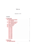
The visrock user manual
Daniel Lübbert
July 23, 2006
(Id: visrockManual.tex,v 1.1 2005/08/02 14:54:41 luebbert Exp )
Contents
1 Introduction - what the visrock program can be used for
1.1 Structure of this manual . . . . . . . . . . . . . . . . . . . . . . . . . . . .
3
5
2 Preconditions to using visrock
2.1 Obtaining visrock . . . . . .
2.2 License policy . . . . . . . . .
2.3 System requirements . . . . .
2.4 Installation . . . . . . . . . .
2.5 Launching visrock . . . . . .
.
.
.
.
.
6
6
6
6
7
7
.
.
.
.
9
9
11
14
15
.
.
.
.
.
.
.
.
.
16
16
16
18
18
22
23
23
24
29
.
.
.
.
.
.
.
.
.
.
.
.
.
.
.
3 Using visrock, I: Basic functionality
3.1 Data input (reading images) . . . .
3.2 Image analysis options . . . . . . .
3.3 Saving the results to disk . . . . . .
3.4 Terminating the program . . . . . .
.
.
.
.
.
.
.
.
.
.
.
.
.
.
.
.
.
.
.
.
.
.
.
.
.
.
.
.
.
.
.
.
.
.
.
.
.
.
.
.
.
.
.
.
.
.
.
.
.
.
.
.
.
.
.
– for beginners
. . . . . . . . . . .
. . . . . . . . . . .
. . . . . . . . . . .
. . . . . . . . . . .
.
.
.
.
.
.
.
.
.
.
.
.
.
.
.
.
.
.
.
.
.
.
.
.
.
.
.
.
.
.
.
.
.
.
.
.
.
.
.
.
.
.
.
.
.
.
.
.
.
.
.
.
.
.
.
.
.
.
.
.
.
.
.
.
.
.
.
.
.
.
.
.
4 Using visrock, II: Advanced functionality – for experienced users
4.1 Curve analysis options . . . . . . . . . . . . . . . . . . . . . . . . . .
4.2 Curve plotting options . . . . . . . . . . . . . . . . . . . . . . . . . .
4.3 Image Plotting options . . . . . . . . . . . . . . . . . . . . . . . . . .
4.4 Axis units . . . . . . . . . . . . . . . . . . . . . . . . . . . . . . . . .
4.5 Histogram display . . . . . . . . . . . . . . . . . . . . . . . . . . . . .
4.6 Line profile extraction from images . . . . . . . . . . . . . . . . . . .
4.7 Correlations . . . . . . . . . . . . . . . . . . . . . . . . . . . . . . . .
4.8 Noise reduction . . . . . . . . . . . . . . . . . . . . . . . . . . . . . .
4.9 Image processing options - sharpening, smoothing and peak detection
1
.
.
.
.
.
.
.
.
.
.
.
.
.
.
.
.
.
.
.
.
.
.
.
.
.
.
.
.
.
.
.
.
.
.
.
.
5 Using visrock, III: Special functions for specific applications
5.1 Functions for Rocking Curve Imaging . . . . . . . . . . . . . . .
5.2 Functions for Tomography . . . . . . . . . . . . . . . . . . . . .
5.3 Functions for Fine-Slicing . . . . . . . . . . . . . . . . . . . . .
5.4 Functions for Small-angle scattering and general Crystallography
5.5 Functions for Detector Calibration . . . . . . . . . . . . . . . .
.
.
.
.
.
.
.
.
.
.
.
.
.
.
.
.
.
.
.
.
.
.
.
.
.
.
.
.
.
.
32
32
33
34
35
35
6 Planned future developments of visrock
38
7 List of known bugs
7.1 Bugs . . . . . . . . . . . . . . . . . . . . . . . . . . . . . . . . . . . . . . .
7.2 Not bugs - features . . . . . . . . . . . . . . . . . . . . . . . . . . . . . . .
39
39
39
8 Impressum
41
9 Literature references
42
2
1
Introduction - what the visrock program can be
used for
The visrock program was written to facilitate the interactive handling and analysis of digital X-ray images. It was originally developed for applications in Rocking Curve Imaging,
but was later extended to several other fields of X-ray imaging. It can be useful in various
applications that are based on linear sequences of 2D images (”sequential imaging”):
Rocking Curve Imaging (RCI): Visualizing the spatial distribution of mosaicity and
lattice quality by a series of plane-wave X-ray diffraction topographs recorded along
the rocking curve of a single crystal [LBH00, MLK03]
X-ray tomography: 3D image reconstruction from a series of projection radiographs
[Her80]. visrock cannot do the reconstruction, but can perform a few tasks for
preparing experimental data for reconstruction and for checking data integrity.
Fine-Slicing (or ”Super-fine Φ slicing”): Measuring the mosaicity of (mostly protein)
crystals along all directions of reciprocal space by simultaneously recording rocking
curves from a great number of crystallographic reflections, using a CCD camera
covering a wide range of exit angles [BSL00].
Diffraction-enhanced imaging (DEI): Recording projection radiographs of a (possibly
non-crystalline) sample with a crystal analyzer as an additional optical element in
the exit beam, at a series of angular positions along the rocking curve of the analyzer
crystal (see e.g. [Pag03]).
Reticulography: Visualizing lattice irregularities in a crystal by monitoring the distortion
of a rectangular grid pattern in X-ray diffraction topographs recorded at several
different sample-camera distances [LM96].
Detector calibration: visrock includes features for testing and quantifying the characteristics of CCD cameras (and other digital area detectors) in terms of reproducibility
and noise level, linearity, sensitivity, and spatial homogeneity of response. These can
be determined from various series of dark field and flat field images.
The visrock program is a graphical user interface (GUI) – it is entirely based on a
point-and-click strategy. The main aim is to simplify tasks that occur frequently and
repetitively in image sequence analysis. No keyboard input of any kind is required – a
simple mouse will suffice as an input device. Among the functions that can be executed in
this way are (sorted roughly from simple to more complex):
• Reading image data from a large variety of file formats.
• Color plotting of (scalar, i.e. intrinsically ”black-and-white”) images to screen or to
postscript output files
3
• Interactively adjustable color scales, either linear or logarithmic
• Plot range selection based on absolute numbers or on percentile values
• Playing movies of image sequences
• Format conversion of grayscale images (e.g. from *.edf to *.png, from *.tif to *.edf,
and many more) – for single images or entire image series
• Interactive zooming (specifying areas of interest with the mouse)
• Monitoring the evolution of the intensity value in individual pixels along an image
sequence (file series), or of the average intensity of a group of pixels (Interactive
extraction of local or regional ”Rocking Curves”)
• Automatic peak detection in extracted profiles
• Determination of peak half widths (FWHM) in profiles
• Gaussian fitting of profile peaks
• Line profile extraction from images, in horizontal or vertical direction
• Horizontal and vertical projections (summation) of image contents
• Image rotations, by arbitrary angles
• Image statistics
• Dark field and flat field corrections
• Renormalization of an image sequence, based on the intensity statistics in a small
region of interest/ROI (e.g. to compensate for a decay in primary intensity)
• Rebinning (in 1, 2 or 3 dimensions)
• Sharpening and smoothing of images
• Noise reduction
• 2D peak detection in images
• Fourier transforms of images (in 2 dimensions)
4
1.1
Structure of this manual
The remainder of this manual is divided into 4 main chapters:
Chapter 2 describes how to prepare for the first use of visrock.
Chapter 3 discusses a first complete round of using visrock, from data input to result
output. It is limited to the absolute essentials, and meant to be short and easy to read. It
should be considered as obligatory reading by every new user of the program.
Chapter 4 provides guidance to the more advanced features of the visrock program.
It covers in detail all the available image analysis, processing and plotting options, and
serves as a reference to those users who want to get the most out of the program.
Finally, chapter 5 covers a few very specific functions related to single scientific applications. It shows how individual task occurring repetitively in some fields of X-ray imaging
may be carried out by visrock.
5
2
2.1
Preconditions to using visrock
Obtaining visrock
The visrock software can be obtained directly from the author, based on a personal
collaboration agreement.
2.2
License policy
The visrock software may be used free of cost and for an unlimited time. However, it
must not be redistributed, nor made publicly available on the internet, on an intranet or
on any other publicly available storage space.
The author will be happy to receive suggestions for new collaborators and users of the
visrock project.
2.3
2.3.1
System requirements
Software requirements
visrock was written in the IDL programming language (see http://www.rsinc.com). The
software is distributed as an IDL *.sav file, which requires a working IDL installation in
order to be run. Ideally, the user’s institution should have an IDL license – which is the
case at almost all synchrotrons, many universities and other research institutions. However,
from IDL version 6.0 on, *.sav files can also be run from unlicensed IDL installations (the
so-called ”IDL Virtual Machine“).
By default, visrock is optimized for the latest version of IDL (version 6.0, as of July
2004).
2.3.2
Operating system
IDL runs on almost any modern operating system (Linux, Unix’es, all kinds of Windows,
Apple, ...). visrock can therefore be run on any type of computer. Only some special
conveniences realized by calls to external programs are limited to Linux/UNIX systems.
The concerns in particular the input of compressed data and the display on screen of
postscript files.
2.3.3
Hardware requirements
RAM: visrock assumes that the entire sequence of images can be loaded into RAM
simultaneously. This is sometimes a very severe restriction to the allowed number of
images and/or pixels.
An example: Even for a well-equipped computer with 2 GB RAM and for images
of 20482 pixels à 2 Bytes (typical case for ESRF-Frelon cameras), this means that
6
no more than 200–230 images can be analyzed at once (leaving some RAM for IDL
itself and other system applications).
Larger sequences can either be analyzed piecewise (e.g. in four ”quadrants”), or on
systems with even more memory (such as the ESRF-indigo machines with 16 GB
of RAM).
Screen: visrock can be run on screens having at least 1024×768 pixels, but is optimized
for larger screens (1600×1200 is ideal).
2.4
Installation
visrock does not need to be installed in any way. Just copy the downloaded file visrock.sav
to the directory of your choice - that’s it.
2.5
Launching visrock
2.5.1
With an IDL license
Start IDL by typing ”idl” on the Unix prompt, or by clicking on the appropriate icon under
Windows.
On the IDL command line, type
restore,’<path>/visrock.sav’
where < path > is the path to the directory where you saved visrock.sav.
Provided that you have correctly set the IDL PATH environment variable, you should
now see the visrock GUI (see Fig. 1).
2.5.2
Without an IDL license
Starting from IDL version 6.0 on, precompiled IDL programs (such as visrock.sav) may
be run in the ”IDL Virtual Machine (VM)” even without an IDL license. For further explanations, see the file idlvm.pdf provided in the help subdirectory of your IDL distribution.
To start visrock in the IDL VM, proceed as follows:
Under Linux: On your command line, type
idl -vm=<path>/visrock.sav
where < path > is the directory where you stored visrock.sav.
7
Figure 1: Appearance of the visrock GUI, in Linux style. The two plot areas are for image
display (left) and curve display (right). The meaning of the remaining buttons and fields
will be explained in subsections 3 and 4.
Under Windows: Drag-and-drop the visrock.sav program onto the IDL-VM icon on
your desktop.
In both cases, you will have to click away the IDL-VM splash screen.
Please be aware that a few limitations exist in the unlicensed mode of IDL, as described
in idlvm.pdf. In particular, IDL’s execute function will not work, which means that
commands entered via the ”execute” text field at the bottom of the visrock window
cannot be carried out.
8
3
Using visrock, I: Basic functionality – for beginners
Basic usage of visrock usually includes three steps: Data input, image analysis, and
output of results (most often as postscript plots).
3.1
Data input (reading images)
The visrock program works on a 3D data set (intensity data as function of e.g. x, y and ω).
These are usually read into memory as a sequence of 2D images (intensity data as a function
of x and y, for one value of ω at a time).
3.1.1
Reading individual images
Single images can be read from hard disk by clicking on the Read CCD-files button, in
the upper right of the visrock GUI. Multiple images can be selected by using the SHIFT
and/or CTRL keys, and will be read in sequence after clicking OK.
3.1.2
Reading large series of images
When reading large series of images, it may be more convenient to specify the images to
be read via a *.txt file containing the names of all the image files, in a single column.
This can be done by clicking on the Read File list button.
3.1.3
Supported image formats
The format of the image files will be automatically analyzed by visrock from the file name
extension. The following image formats are understood by visrock:
*.tiff: Standard digital image format.
*.jpg: Standard digital image format.
*.gif: Standard digital image format.
*.png: Standard digital image format.
*.edf: Esrf Data Format, produced by 2D detectors such as the ”Frelon” cameras. ASCII
header, plus uncompressed binary image data.
*.mccd: Image format produced by MarReserach CCD cameras, in widespread use in
protein crystallography. Regular tiff format, plus extra binary header.
*.b16: Slightly exotic digital image format, apparently produced by CCD cameras from
PCO.
*.gqe: Binary image format produced by the Spectra program, developed by Thorsten
Kracht and used at many HASYLAB beamlines.
9
*.xdr: Even more exotic general file format, somehow device-independent, read and written by older IDL programs (in use at BW4@HASYLAB).
In addition to the above (and as a default, if the file name matches the standard for
none of the above), visrock can analyze a general binary image format, consisting of a
H-Byte header (which will be ignored) plus a rectangular array of N×M pixels, with L
Bytes per pixel. The integer numbers H, N, M and L will be requested interactively until
the expected number of Bytes (N*M*L+H) matches the actual file size.
As an extra feature, visrock can read compressed (zipped) copies of all available
image formats. This will work primarily on Linux systems; it may or may not work under
Windows. It is particularly useful with *.edf images, which are uncompressed in their
native form (unlike *.jpg or *.png) and therefore waste enormous amounts of hard disk
space.
Currently, *.gz and *.bz2 compressed formats are supported. When visrock encounters a compressed image, it is first uncompressed to a temporary file, and then read as
usual. Decompression is usually rather fast (some tenths of a second), even if the original
compression took considerably longer.
Note that for this to work, two conditions must be fulfilled:
• The appropriate decompression program must be found in the PATH (gunzip or
bunzip2).
• You must have write permission on the /tmp directory.
3.1.4
Input details
After selection of the files to be read, a few more details of the reading process can be
specified in a separate window (see Fig. 2). From top to bottom, the most important
choices are (all parameters must be integer numbers):
bin factor: Rebin original images, i.e. reduce their number of pixels via averaging, by
this factor. The x- and y- dimension will be treated alike, i.e. reduced by the same
factor. Must be an integer.
use every Nth file only: Read only image files nr. 0, N, 2N,... and disregard files nr.
1 − (N − 1) etc. Helps to save RAM, and considerably speeds up the reading process
(by at least a factor N). Must be an integer.
wait time: If the next file to be read is not found on hard disk (e.g. because it is just being
read out from the camera), wait x seconds and try again before giving up. Helpful
when starting a reading process while the series of images is still being recorded.
x-start, x-stop, y-start, y-stop: Keep only a restricted area of the original images
in memory, and discard the outer regions. Helpful in order to save memory space
when the features of interest occupy only parts of the image surface. Values must be
∈ [0, N − 1].
10
Figure 2: Popup window allowing to specify details of the image reading process.
The remaining fields of the window shown in Fig. 2 will be discussed in Chapter 5.
3.2
Image analysis options
In the left drawing area, 2D maps can be plotted which represent sections or projections
from the 3D data block that resides in the program’s memory. A large number of options is
available, as can be seen from the list below. The first three options represent sections from
the original data, whereas all the remaining options represent composite images generated
from the entire stack of data, mostly by projection along the third (angular) dimension.
x-y (Single images): Show one of the original images. Its number is selectable via the
slider at the bottom of the GUI.
x-z (x-omega): Show a section from the 3D data block, perpendicular to the original
image planes. This is a sinogram in the case of tomography with vertical rotation
axis (along y).
11
y-z (y-omega): Show a section from the 3D data block, perpendicular to the original
image planes. This is a sinogram in the case of tomography with vertical rotation
axis (along x).
integrated Intensity: For each pixel, show the sum of intensities across the entire image
stack.
maximum Intensity: For each pixel, show the maximum intensity reached anywhere
across the entire image series.
maxpos: For each pixel, show the angular position (or image number) where the miaximum is reached.
minimum Intensity: For each pixel, show the minimum of intensity reached anywhere
across the image series. Rarely used; sometimes useful with tomography images.
minpos: For each pixel, show the angular position (or image number) where the minimum
is reached.
Int and Pos: Under development, no documentation yet. Don’t use.
FWHM: For each pixel, calculate the full-width-at-half-maximum of the main peak in
the local intensity curve.
FW percent M: For each pixel, calculate the full width at x% of peak height, with
selectable percentage x. For x = 50, the result is identical to FWHM. Sometimes more
representative than the FWHM map in case of multiple peaks or peaks with broad tails.
ratio FWHM / FW percent M: Quotient of the latter two quantities. Sometimes useful to detect regions with different numbers of peaks (overlapping grains in RCI).
I integr.d-restricted range: Summation of intensity across a restricted range of image
numbers only, rather than the entire series. Will ask for numbers of first and last
image. Useful when multiple peaks exist for each pixel.
maximum-restricted range: Similarly for maximum intensity.
maxpos-restricted range: Similarly for position of maximum.
FWHM-restricted range: Similarly for peak FWHM.
Angular center of mass: For each pixel, calculate the center of mass of the associated
intensity distribution as a function of angle or image number (the I(ω) distribution).
Result is in units of angle. Alternative to maxpos, statistically more robust: The
resulting angle is slightly less sensitive to noise than maxpos.
12
Angular standard deviation: For each pixel, calculate the standard deviation of the
local I(ω) distribution. Result is in units of angles, and is a measure of peak width.
It is a statistically more robust alternative to FWHM, which may be preferable in case
of noisy data, multiple peaks, and/or peaks with broad tails.
N peaks: Calculate the number of peaks in each local intensity curve. Calculation based
on the algorithm described in [Sil96].
Average: For each pixel, calculate the average intensity across the image series.
Median: For each pixel, calculate the median intensity across the image series.
max-min: For each pixel, calculate the difference between maximum and minimum intensity across the image series. Sometimes useful for tomography data.
Standard deviation: For each pixel, calculate the standard deviation of the associated
vector of intensity values. Result is in terms of intensities. High values indicate that
something changes somewhere in the entire series.
I over sigma: Ratio of average intensity over intensity standard deviation for each pixel.
noise <=> Poissonian?: Intensity standard deviation divided by square root of average
intensity, for each pixel. Useful when evaluating the homogeneity of a series of flat
field images.
wafer present yes no: Binary image (yes/no) indicating which pixels “looked” on diffracting material (yes) or air (no). Calculation based on selectable upper/lower limits for
FWHM and max Int. Must have been calculated before using the mask wafer area
button, located on the right side of the visrock GUI.
threshold: Binary image (yes/no) showing where maximum Intensity exceeded a selectable threshold.
Gauss fit max Int: Apply Gaussian fit to (highest) peak in each pixel’s intensity distribution, and display the peak height of the fitted curve. Robust alternative to
max Int, less sensitive to noise.
Gauss fit max Pos: Similarly, display angular peak position of fitted curve.
Gauss fit FWHM: Similarly, display half width of fitted curve. Very interesting alternative to FWHM: less sensitive to noise, and less prone to errors due to discrete scan
step width.
Linear fit: Background: Apply linear fit to local intensity distribution, and display
residual (fitted intensity for ω = 0). Useful mainly for detector calibration purposes.
Linear fit: Slope: Similarly, display slope of linear curve.
13
Linear fit: Chi2 : Display chi-square for local fit. High values indicate deviations from
linear local curve shape.
Linear fit: Status: Check result of local fit (0 for success, 1 for error, 2 for inaccurate
result).
3D-Intensity: Display the entire 3D data block, similarly to volume data in tomography.
3D-Peak locations: Undocumented feature.
Principal components: Apply principal components analysis to the image stack. This is
a standard procedure in multivariate (multi-dimensional) statistics: A new, rotated
coordinate system is introduced in such a way that the first components of the (new)
data vectors contain a maximum of the total variance of the data, and the last
component a minimum.
For application to an image series, the image number is regarded as the “component
index” of the data “vector”, and each pixel as an independent measure of the same
“vectorial” quantity. The “coordinate transformation” creates a new set of images,
the first of which has a maximum of contrast, whereas the last ones are rather “flat”.
This algorithm is a rather efficient method for contrast enhancement, but somehow
dissatisfactory for quantitative imaging in the sense that the intensity values of the
resulting images do not have any clearly defined unit.
3.3
3.3.1
Saving the results to disk
Postscript output
As soon as satisfactory plots of the relevant quantities have been obtained in the two plot
areas in the visrock GUI, the images can be output almost identically to postscript files.
To that end, click the Map− > ∗.ps and/or Curve− > ∗.ps buttons in the top row of the
visrock GUI. A default filename wil be suggested, containing quite detailed information
on the kind of plot. The type of postscript plot (encapsulated yes/no) will be adapted to
the final filename chosen (*.ps or *.eps).
On appropriate operating systems (Linux/UNIX), the newly created postscript file will
be opened in ghostview for immediate checking/printing.
3.3.2
Data output
The results displayed in the plotting areas may as well be saved as raw data, for later
display with other programs than visrock. To that end, click the Map− > ∗.img and/or
Curve− > ∗.dat buttons in the top row of the visrock GUI. Maps can be stored in
(almost) any of the image formats discussed in section 3.1.3. Curves will be saved as ascii
files, with two data columns and one row for each image in the series.
14
3.4
Terminating the program
When your work is done, terminate the program by clicking either the Quit or the Exit
button in the upper left of the visrock GUI. The former will close the GUI, but leave the
IDL session open, with the values of various variables still in memory. The latter will close
the IDL program as well and exit to the Linux shell / Windows desktop.
15
4
4.1
Using visrock, II: Advanced functionality – for experienced users
Curve analysis options
When the user clicks on a pixel in the map plotting area, a curve plot (intensity versus
angle/image number) will be displayed in the second (right) plotting area. The scaling
of the x axis of the curve can be selected via the ”Delta-omega” input field in the top
row of the visrock GUI: If a value of 1 is entered, the x axis can be interpreted as image
numbers; if the angular increment used in the scan is entered, the x axis can be interpreted
as angles. The ”Start omega” input field can be used to select an angular offset (i.e. a
shift of the entire x axis).
The exact meaning of the y-axis of the curve depends on the setting of the option
selected in the curve analysis droplist just below the plot. The following functions are
available:
orig data: Plot the intensity data contained at the respective pixel position in the original
images, as a function of image number/angular position.
ROI-integral: Plot the sum of intensity values in all pixels visible in the map plotting
area. When the map is in the completely unzoomed state, the sum of intensities in
the entire image(s) is plotted.
ROI-min: Plot the minimum intensity value reached in any pixel across the current zoom
area, as a function of image number/angular position.
ROI-max: Plot the maximum intensity value reached in any pixel across the current zoom
area, as a function of image number/angular position.
spatial stddev: Plot the standard deviation of intensity values in a local surrounding of
the pixel selected by clicking, as a function of image number. Useful e.g. for investigating whether the ”noisyness” of a camera image changes with time or temperature.
When this option is selected, an additional ”stddev radius” input field will appear
below the plot, allowing to select the width of the local surrounding (with a standard
value of 1 pixel to the right and left).
sum x( -log( data)) for ROI: Expert feature, undocumented so far.
sum y( -log( data)) for ROI: Expert feature, undocumented so far.
4.2
Curve plotting options
The appearance of the Intensity-versus-angle curves displayed in the right drawing area
can be changed via the buttons below the plot.
16
Figure 3: Curve plotting options
4.2.1
Plot range selection
The button labeled ”log” allows to change back and forth between linear and logarithmic
intensity scale.
The button labeled ”Full range” determines the range of values shown on the y (intensity) axis: When the button is not pressed, the y range is individually adapted to the
actual curve, thus maximizing the visible ”contrast”. When the button is pressed, the y
range is determined from the minimum and maximum values in the entire 3D data block.
This facilitates the comparison (on an absolute scale) of several different extracted curves,
obtained by clicking in sequence on different pixels in the map.
4.2.2
Peak detection
The button ”show peaks”, when pressed, will activate auomatic peak detection in the
current curve. ”Real” peaks (as opposed to local absolute maxima) will be marked by a
sign. This serves mainly as a control mechanism for the ”N peaks” analysis option in map
display.
Peak detection is based on a curve sharpening algorithm (see [Sil96]) followed by a
search for local maxima in the sharpened curve. Maxima must be higher than adjacent
minima by a factor that can be regulated via the ”peak detect.max ratio” input field.
The sharpened curve as an intermediate step towards peak detection can additionally be
displayed by pressing the ”show sharp” button.
17
4.2.3
Curve shape analysis
Curve shapes can be analyzed either by a phenomenological determination of half-widhts
(button FWHM) or by fitting with a linear (button ”Lin.Fit”) or Gaussian (button ”Gauss-Fit”)
model. In all three cases, the resulting parameters will be displayed in a corner of the plot.
4.2.4
Noise reduction
The ”median filter” button will apply a one-dimensional median filter to the current
extracted curve. This will smoothen local spikes and reduced noise, but also flatten ”real”
peaks and (slightly) reduce resolution along the x direction. The width of the filter window
can be regulated via the ”smooth-/median-width” input field.
The ”Dezinger” button will try to reduce noise from extreme intensity values in individual positions (”zingers”) by applying a statistical criterion [BTG99]. This is mainly
meant as a control facility for the ”Dezinger” option in map plotting, which works according
to the same algorithm.
4.2.5
Other plot options
Pressing the ”oplot” button allows to plot a new curve without erasing the old one. This
facilitates comparison of curves extracted from several different pixels.
When the ”VBar” button is activated, a vertical red line in the curve plot indicates the
angular position (image number in the series) at which the picture presently displayed in
the map plot area was taken.
4.3
Image Plotting options
4.4
Axis units
The x and y axes in the map display can be labeled by physical units rather than pixel
numbers. To this end, select ”Edit plot options” from the Extra-functions menu. In
the extra window that appears (see Fig. 4), select appropriate values for the variables
”X UNIT NAME” and ”X SCALE FACTOR” (the length of one pixel, in the unit defined by
X UNIT NAME), and similarly for y.
The same window also allows to select the character size to be used in the two displays
and in the legends, and to switch on (1) or off (0) the display of various titles and subtitles.
Finally, the nature and format of the map legend display can be influenced via this window.
4.4.1
Color scale / Plot range selection
The color scale in the maps can be adjusted so as to maximize contrast and highlight
specific features. Three mechanisms are available: One can either enter lower and upper
limit values manually in the fields labeled ”Minimum value:” and ”Maximum value:”. As
a consequence, any pixel values beyond these limits will be represented with the same
18
Figure 4: The ”Edit Plot Options” window, allowing to define axis units, among others.
color as the limits themselves. In this way, the entire range of available colors (contrast)
is concentrated on this interval of values.
As an alternative, the values can be defined interactively by using the two vertical
sliders to the left of the map plotting area.
The third, most ”automatic” way is to define min and max values in terms of percentiles: After entering the required numbers in the fields labeled ”Minimum percentile”
and ”Maximum percentile” (see Fig. 5) the program will automatically translate these
into limits in terms of absolute pixel values. Percentile values must lie between 0 and
100. As an example, min and max percentiles of 5 and 90 mean that the lowest 5% and
the highest 10% of pixel values will be ”flattened” (mapped to the corresponding limiting
color). This is particularly useful when a small number of outlier pixels (”zingers”) would
otherwise spoil the automatic selection of color scales.
19
Figure 5: Map plotting options (selection).
4.4.2
Linear/logarithmic scaling. Aspect ratio
When the button ”Map: log” is pressed, the color scale of the map shown in the left
plotting area is chosen on a logarithmic scale. This allows to obtain more image contrast
in regions of weak intensity. Choosing log-scaling will cause problems when parts or all of
the map are in the negative-value range (as may happen for position-of-maximum maps,
for example).
When the button is not active, the color scale is chosen linearly; this will enhance the
visibility of the strongest peaks.
The button just below it, labeled ”1:1”, will activate the ”maintain-aspect-ratio” function. This means that images with different numbers of pixels along the x and y axes will
be plotted in a rectangular area, with dimensions on the screen (roughly) proportional to
the respective number of pixels.
When this button is not active, images will be plotted in a quadratic regions on screen,
often making better use of the available display space.
4.4.3
Zooming and unzooming
By default, all of the available image information is represented in the display. Details can
be magnified by choosing an area of interest (AOI). An AOI is defined interactively by
clicking with the mouse: Place the mouse pointer over one of the corners of a rectangular
AOI, press the middle mouse button (or, in case your mouse has only two buttons, the
left and right buttons simultaneously), move the mouse pointer to the diagonally opposed
corner of the AOI to be defined while keeping the button(s) pressed, and release. During the
move, the present size of the AOI just being defined will be visible as a bright rectangle
overlaid on the image. After releasing, the new (magnified) plot will automatically be
displayed on screen.
The center of the zoomed area can be shifted in the horizontal, vertical or any diagonal
direction by using the ”transfer buttons” (see block of 3 × 3 buttons in the lower right of
Fig. 3). This will leave the magnification (zoom factor) unchanged. An exception is the
central button (labeled ”o”), which will not shift, but increase magnification by a factor 2
in both directions.
The inverse operation – unzooming, i.e. demagnification by a factor of 2 – is performed
by clicking once with the middle mouse button.1 The clicked pixel will become the center
1
More exactly: Clicking and releasing on the same pixel, without intervening motion.
20
of the new image, which will be twice as wide and high as before (provided that enough
data are available).
A double-click with the middle mouse button will perform a complete unzoom, i.e. all
of the available data will be displayed on screen.
Figure 6: Arrow buttons for shifting the region of interest
In order to shift the region of interest to an adjacent area without changing the scale
(magnification factor), use the ”arrow” buttons (Fig. 6). The outer 8 buttons allow to
shift the region horizontally, vertically or diagonally. The central button (labeled ”o”) will
zoom in by a factor of 2.
4.4.4
Mirroring / Image inversion
The map display can be mirrored in either the x- or the y-direction by activating the
”Invert x” and/or ”Invert y” buttons (see Fig. 5).2
4.4.5
Image rotation
The map display can be rotated by an arbitrary angle, by entering a value in the field
labeled ”Rotate by (deg):” – see Fig. 5.
Note that in the case of rotation by ”odd” angles parts of the display area may be void
for lack of data, will parts of the available data disappear beyond the border of the plotting
area.
4.4.6
2D Fourier transforms
Instead of the ”original” data, their 2D Fourier transform data can be displayed in the
map plotting area. Fourier data are complex numbers, so the user can choose to plot the
real or imaginary part, or their absolute values. This choice is made via a droplist on the
right of the map plotting options (see Fig. 5). TODO: Fourier-droplist abbilden.
2
Note that when any one of these two buttons is active, value and profile extraction from the map by
mouse clicking will not work (at least in the present version of visrock).
21
4.5
Histogram display
Figure 7: Histogram display
The ”Show histogram” button (see Fig. 1) allows to display a statistic of pixel values
and their frequency of occurrence in the current image (i.e. a histogram of pixel values
in the plotting area). The histogram is taken only over the currently zoomed region, and
thus changes with the zoom state (center and magnification factor). A separate window
(see Fig. 7) containing the histogram plot will be opened, which can be kept open for later
use if required since it does not block action in the main window. A few buttons allow to
manipulate the histogram plot:
”Save this plot”: Output the plot to a postscript file. A default filename of ”tmp.ps”
will be suggested, but can be changed before final confirmation.
”Save these data”: Store the plot data to an ASCII data file. A default filename of
”tmp.dat” will be suggested, but can be changed before final confirmation. The file
will contain two columns of data, and one row for each data point in the plot.
”Real data”: Plot the original histogram data (default).
”Fourier data”: Plot the 1D Fourier transform of the original data (rarely useful for
histogram data).
xlog: Logarithmic x-axis (axis of pixel values).
ylog: Logarithmic y-axis (axis of frequency of occurrence).
22
Figure 8: Some map analysis functions.
FWHM: Automatically analyze the width of the highest peak in the plot, and write the result
to a corner of the plot
”min” and ”max”: Specify a restricted range for the y-axis, in absolute frequency-ofoccurrence numbers.
4.6
Line profile extraction from images
One-dimensional value profiles can be extracted interactively from the 2D map plots via
mouse clicks: A double-click with the left mouse button will extract a horizontal line profile
(z values as a function of x coordinate) from the map, crossing the clicked pixel. A doubleclick with the right mouse button will extract a vertical line profile (z values as a function
of y coordinate).
4.7
Correlations
Correlation coefficients measure the degree of similarity between two images. They can
have values between 0 (no similarity) and 1 (complete correspondence).
Correlation functions are a more general concept, telling whether two images can be
made to be similar after a lateral (2D) shift.
4.7.1
Correlation coefficients and R-values
The button labeled ”Correlation coefficients” will trigger the calculation of correlation coefficients between any pairs of images in the series of N images currently loaded into
memory. The result is a (real and symmetric) N × N matrix of correlation coefficients,
which will be displayed as a 2D map in a separate window (see Fig. 9).
This function is useful e.g. when inspecting a series of flat field images in tomography,
which should all be representing the identical distribution. Considerable ”breaks” in the
2D field of correlation coefficients may indicate an uncontrolled change in experimental
conditions during exposure of the flat field series.
A similar concept, well-known to crystallographers, are the so-called ”R-values” between pairs of images. They are calculated by pixel-wise summation of relative differences
between pixel values in the two images. One of the images is defined as a reference, while
the other is the ”sample”. Therefore, the resulting N × N matrix is asymmetric. Apart
from this, the result is mostly equivalent to the case of correlation coefficients, with the
difference that R-values are additionally sensitive to changes in overall intensity values.
23
This function may therefore be useful to detect e.g. a sudden partial beam loss during
exposure of a flat field image series.
4.7.2
Correlation functions
A correlation coefficient between a pair of images is a single (scalar) number, whereas a
correlation function for a pair of digital images is again a 2D distribution, with the same
number of pixels in x and y as the original images. The central element has the same value
(between 0 and 1) as the ”trivial” correlation coefficient, while the value of all other pixels
indicate how much similarity could be achieved by shifting one of the two images by the
corresponding number of pixels with respect to the other.
Clicking on the button labeled ”Correlation functions” allows to calculate a correlation function between the currently selected image and a second one, to be selected
from a list of filenames presented in a new window (see Fig. 11). After confirmation and
calculation (which may take some time), the resulting 2D correlation function is saved as a
postscript file, which will be displayed on screen using ghostview (on Linux/UNIX only).
As the correlation function has complex values, there will be several plots presenting the
real and imaginary components as well as the absolute values as 2D distributions, and
several 1D projections of the same data (see Fig. 12).
4.8
Noise reduction
Fig. 13 shows the various options available for suppressing noise in 2D images inside
visrock.
4.8.1
2D Median filtering
Median filtering is a well-known technique for suppressing ”extreme” pixel values in 2D
images. Every pixel value is replaced by the median of all pixel values inside a square box
surrounding the respective pixel. The width of this box can be selected via the field labeled
”Median: x/y=”, and must have a value of 2 or higher. The default value of 0 indicates
that no median filtering will be applied.
Median filtering is rather efficient at eliminating spurious features (single outliers or
small groups of outlier pixels). It has the additional advantage of having rather limited
”collateral effects”, as compared to other averaging and smoothing techniques. It will,
however, slightly degrade the lateral resolution in the image, especially at larger box widths.
2D median filtering is a reversible technique inside visrock in the sense that it is
applied ”on-the-fly” only to the intermediate data just being plotted to screen (or saved
to file), i.e. to the image analysis results, and not to the original image data residing in
memory. Therefore, reverting to a width value of 0 will reproduce exactly the original,
noisy data.
This convenience comes at a price in terms of efficiency: The median filtering operation
is carried out anew every time that the image is being plotted. This takes a little time (on
24
Figure 9: Map of correlation coefficients between pairs of images from a series of 10 primary
beam images. Both the x and the y axis are in terms of image numbers, defined from 0 to
N − 1. Note that the distribution is symmetric, and that values on the diagonal are equal
to 1.00 – simply indicating that each image is identical to itself. The non-diagonal values
show that images nr. 0–7 are rather similar to each other, whereas images 8 and 9 deviate
more strongly. The 2×2 fields in the upper right corner show that these last 2 images are
again rather similar to each other. In summary, beam conditions stayed constant until
image nr. 7, after which an (unknown) sudden slight change occurred. The nature of
this change may be further elucidated by other functions of the visrock program. As an
example,the correlation function between e.g. images 6 and 8 may give hints whether a
(lateral or vertical) shift of beam or camera gave rise to the change.
25
Figure 10: Map of ”spatial R-values” between pairs of images from a series of 12 dark
field images. Note again that values on the diagonal are trivial – with an R-value of 0.00
being equivalent to a correlation coefficient of 1.00, both indicating identity. Note also that
unlike the previous figure, this distribution is not symmetric.
26
Figure 11: File selection widget, allowing to select a second image with which the one
presently displayed is to be correlated.
the order of seconds). To accelerate the procedure, the median filtering can alternatively
be applied to the original image data by pressing the ”Apply to all data” button after
entering the appropriate box width values. Be aware that this operation is irreversible
(unless you are willing to read all the images again from hard disk).
4.8.2
3D median filtering
When using ”Apply to all data” for median filtering of the original image data, an
additional and independent box width can be entered into the field labeled ”z=”. When
a value ≥ 2 is entered, an additional 1D median filtering operation will be applied to the
pixel value array along the z direction (the ”rocking curve”) at each 2D pixel location.
This operation relates the values in adjacent images to each other, unlike the 2D filtering
operation that is applied to each image separately (and is carried out first).
4.8.3
”Dezingering”
The field labeled ”Dezinger”, when filled with a value > 0, will activate the ”Dezingering”
function. This is a noise reduction technique that tries to eliminate spurious high pixel
values (”zingers”) based on a standard deviation criterion. The value entered roughly represents a multiple of standard deviations that can be tolerated as ”statistical” deviations;
more highly deviating values will be eliminated.
For this to work, a set of N (at least 2) independent images theoretically representing the identical ”true” image, but distinct due to noise, are required. This function is
particularly useful for treating dark field or primary beam images.
The algorithm is based on [BTG99], assumes spatial homogeneity of ”noisyness”, and
works iteratively until convergence is achieved and a best compromise image is found. The
calculation works independently for each pixel in the images; adjacent pixels are not related
to each other.
27
Correlation function, real part (lin. scale)
Correlation function, absolute value (lin. scale)
300
300
200
200
−0.1332
−0.1023
−0.07131
−0.04034
−0.009372
0.02160
0.05256
0.08353
0.1145
0.1455
0.1764
100
0
1.053E−07
0.01764
0.03529
0.05293
0.07057
0.08822
0.1059
0.1235
0.1411
0.1588
0.1764
100
0
−100
−100
−200
−200
−300
−300
−200
−100
0
100
200
−200
−100
0
100
200
Correlation function of /home/luebbert/Data/1999/06_99/caf−C.0006.edf.gz vs. /home/luebbert/Data/1999/06_99/caf−C.0008.edf.gz
Correlation function of /home/luebbert/Data/1999/06_99/caf−C.0006.edf.gz vs. /home/luebbert/Data/1999/06_99/caf−C.0008.edf.gz
Sum of correlation values (real part) over y
Correlation map, projected onto x shift axis
60
40
20
0
−20
−40
−200
−100
0
100
200
x
Correlation function of /home/luebbert/Data/1999/06_99/caf−C.0006.edf.gz vs. /home/luebbert/Data/1999/06_99/caf−C.0008.edf.gz
Figure 12: Result of calculation of correlation function between a pair of images: Full
correlation function (real part), full correlation function (absolute value), and projection
onto the horizontal axis.
4.8.4
3D variance filter
Unlike Dezingering, the ”3D variance filter” function for noise reduction will combine the
values of several spatially adjacent pixels: For each pixel, the average and the standard
deviation of pixel values in a local environment (cube of 3 pixels side length) is calculated
and compared to the central pixel. If the pixel value deviates from the average by more
than and (interactively entered) tolerance value times the standard deviation, then it is
replaced by the mean.
This algorithm is realized in two alternatives: The ”parallel” version treats all pixels
identically, and always takes the original pixel values when calculating the local environment values. The ”serial” version immediately takes the new values into consideration
when treating the local environements for the next pixel, as it works its way through the
entire data array.
Both variants are rather efficient at eliminating ”real” outliers (and only those). However, they are pretty demanding in terms of computing time and (particulary) working
memory: Saving of intermediate results will require a maximum of 6.5 times the memory
space occupied by the original image data. As an example, if you are treating an image
28
Figure 13: Noise reduction options.
series with 100 MB of data, and you don’t have at least 650 MB of RAM, better don’t use
this function.
4.8.5
3D smoothing
A more basic way of 3D noise reduction is realized by the ”Smooth:” fields: 3 numbers can
be entered here, which represent the lengths along the 3 coordinate axes of a box around
each pixel. Values inside this box are averaged, and the average value assigned as a new
value to the central pixel. The result of this function is similar to using the ”3D variance
filter” with a tolerance level of 0, but more efficient in terms of execution time and memory
requirements.
4.8.6
3D rebinning
When the ”rebin” option rather than the ”smooth” option is selected, the same smoothing
mechanism will result in a new data block with reduced dimensions, i.e. smaller numbers
of pixels along the three axes (by factors corresponding to the values entered into the three
fields).
Note that these last two functions are irreversible, unless you are willing to read the
original images again from hard disk.
4.9
Image processing options - sharpening, smoothing and peak
detection
visrock can perform a number of image processing options on the data to be displayed in
the map plotting area:
Original data: No image processing operation.
Deriv x: Show (discrete) derivative of image data along the horizontal axis, instead of
the original image. In other words, replace pixel value ui,j by ∂x u = ui+1,j − ui,j .
Deriv y: Similarly for the vertical direction
Modulus of Gradient:
Absolute value of the 2D vector constructed from the two derivaq
2
(∂x u) + (∂y u)2 . Good for detecting areas of fast changes in image
tives, i.e.
contents.
Phase of Gradient: Direction of the same vector, in [0, 2π]. Often not very useful.
29
Laplace 1: Convolution of original image with a

0 −1
−1 4
0 −1
3×3 kernel given by

0
−1 .
0
Good for detecting (local) peaks in the image.
Laplace 2: Convolution of original image with a

−1 −1
−1 8
−1 −1
3×3 kernel given by

−1
−1 .
−1
Also good for detecting (local) peaks in the image.
Laplace 3: Convolution of original image with a

1 −2
−2 4
1 −2
3×3 kernel given by

1
−2 .
1
A third way of detecting (local) peaks in the image. For details on the relevant
differences between the three, see e.g. [Pra91].
Peaks: Smooth+Laplace1: First smooth image by a median filter of a given width,
then perform peak detection (as in “Laplace 1”). Good for distinguishing noisy and
spurious local peaks (which will be levelled out by the smoothing operation) from
“real” ones.
mean-local: Convolution of original image with

1 1
1
1 0
8
1 1
a 3×3 kernel given by

1
1 .
1
Replaces each pixel by the average value of its 8 nearest neighbours. Good for image
smoothing, and as a preparation for the signal-mean-local operation.
signal-mean-local: Similar, but additionally subtracting the value of the central pixel
itself. Good for detecting prominent pixels that are very different from their local
surroundings.
stddev-local: For each pixel, calculate the standard deviation of values of the 8 nearest
neighbours, again by convolution. Good for detecting areas of strong local changes,
and as a preparation for SNR-local.
30
SNR-local: For each pixel, calculate the local signal-to-noise ratio by dividing signal-mean-local
by stddev-local. Helps to identify “real” (local) peaks in noisy images, by showing
which pixels exceed their surroundings by more than the local noise level.
This list is of course very incomplete, compared to the many miraculous procedures
contained in books like [Jäh02]. A few additions, like high-pass and low-pass filters, will
be inserted in the near future. Further suggestions from users are always welcome.
31
5
Using visrock, III: Special functions for specific applications
visrock contains a few functions which are individually optimized for very specific applications, and may well be ignored by general users.
5.1
5.1.1
Functions for Rocking Curve Imaging
Dark field correction
In rocking curve imaging (as in tomography, and presumably most other fields of X-ray
imaging) it is important to subtract an image of ”dark counts” – caused by camera dark
current, readout noise, intentional offset etc. – from each one of the actual experimental
images. This task can be automated by using the field labeled ”Dark field:” in the upper
left of the visrock GUI.
The name of an image file containing a dark field image can either be entered directly
into this field via the keyboard, or selected interactively from a list of files on hard disk
via the button on the right. The dark field filename must be entered before reading the
actual (non-dark) image files. The dark field data will be read into memory and displayed
on screen for immediate check. Upon completion of the reading process of the main list
of images, the dark field data will then be automatically subtracted from each and every
image in the series before further processing. This may take some time, depending on the
computer system being used.
Instead of a single dark field file, the user can alternatively specify a set of N dark
field files simultaneously (e.g. by holding the SHIFT and/or CTRL-buttons pressed while
selecting files). These will be understood as several (noisy) instances of the same basic
image, and will be merged into a single ”denoisified” dark field using the ”Dezingering”
algorithm described in section 4.8.3.
5.1.2
Masking sample areas
In Rocking Curve Imaging, the diffracting sample areas often cover only part of the
camera’s field of view. The non-diffracting parts appear very noisy, particularly in the
position-of-maximum and FWHM maps (since the analysis is carried out on spurious peaks).
To mask out these areas (i.e. plot them in the background colour), the ”Mask wafer area”
can be used.
In order for this to work, the ”wafer present yes no” analysis option must have been
selected first. This will carry out an analysis of each local rocking curve and decide
whether it corresponds to diffracting material, based on two criteria: maximum Intensity
and FWHM. These two quantities must lie between respective minimum and maximum
values, which can be entered interactively. As a result, a binary map (1 = diffracting, 0 =
non-diffracting) of the sample area will be displayed.
32
The limiting values can optionally be changed and analysis repeated (e.g. by pressing
the ”replot” button) until the binary image matches expectations. When this is the case,
these data can be used for embellishing other plots by pressing the ”Mask wafer area”
button and then selecting the corresponding analysis option.
5.1.3
Correction of maxpos maps for dispersion effects
The position-of-maximum maps in Rocking Curve Imaging only partly reflect the sample
curvature, since they also contain instrumental effects. In order to correct for this, the ”Do
corr. resol.” button can be used. Note that this button is available only when the
”maxpos” analysis option is active.
After activating the correction option, the program will ask for input data describing
the experimental circumstances (monochromator, sample, reflections, geometry...). After
confirmation, visrock will calculate a correction map, display it as a postscript file, and
subtract it from the raw maxpos map. The correction can be undone by pressing the
”Don’t corr. resol.” button.
The calculation is based on the following formulae:
(To be completed).
TODO: Explain angular correction
TODO: Bild einbinden
Figure 14: Input window for parameters describing the experimental geometry.
5.2
Functions for Tomography
visrock does not perform 3D reconstruction from projections. This can be done by programs like HST. However, visrock can be used for preparing experimental projection images
for reconstruction by HST. This is particularly useful when working at beamlines which are
not (yet) optimized for tomography, where unexpected misbehaviour of optics, rotation
axes and/or detectors may may prevent successful reconstruction unless it is diagnosed
and documented.
5.2.1
Flat field calibration
A flat field correction can be performed automatically, similarly to the case of dark field
correction described above. The name of one or several primary beam images must be
entered into the field labeled ”Prim. beam:” before reading the main series of images.
After reading and (possibly) dark field correction, the experimental images will then be
divided by the primary beam data. Note that this entails a change of data type, which in
many cases means increased memory requirements (e.g.: changing from unsigned short
to float means a doubling of RAM space).
33
5.2.2
Correction for primary beam decay
At most synchrotron sources, the primary beam intensity slowly decays between injections.
To correct for this decay in the series of projection images, proceed as follows:
Select an area in the images which is illuminated by the beam, but never ”sees” the
sample. This can most easily be verified by switching to minimum Intensity analysis
mode. Zoom to exactly this area, and switch to ROI-Integral curve analysis option. If
the curve displayed in the curve drawing area is rougly constant, no correction is necessary.
Otherwise, use ”Normalize to ROI as background” function (in the ”extra functions”
droplist) to correct the entire set of images for the visible decay. After this, the curve on
display should be exactly horizontal.
5.2.3
Sinogram display
Sinograms can be displayed by using the x-ω image display mode (for vertical rotation
axis), or y ω-mode (in the case of a horizontal rotation axis). Starting from an individual
projection image, click anywhere into the image with the left mouse button. This will have
the effect of fixing the y position (for x − ω-mode, or the x position for y − ω-mode) at
which the sinogram is to be taken. Then, switch to the appropriate image analysis mode.
Note that in these modes, the image-number slider (at the bottom of the visrock GUI)
will change values and function, now allowing to switch to different x (or y) positions /
sinogram numbers.
5.2.4
Finding the location of the rotation axis
To find the location (in pixel units) of the rotation axis (horizontal or vertical) in a stack
of tomographic projections, proceed as follows:
In sinogram display, identify one strongly absorbing feature. Take the average between
the x (or y) positions at ω = 0◦ and ω = 180◦.
5.2.5
Zero padding
In case the illuminated area in the experimental projections is not symmetrical around
the (newly found) rotation axis, the image area can be extended by filling with zeroes
(in logarithmic absorption mode, or equivalently ones in transmission mode). TODO:
Explain how!
5.2.6
Detecting axis wobble
TODO: Discuss the extra functions in curve analysis (expert features...).
5.3
Functions for Fine-Slicing
The Fine-Slicing part of visrock is in many ways similar to the Beamish program [LSP00],
although it is based on xds rather than on mosflm).
34
The main idea of the method is to collect rocking curves for many crystallographic
reflections simultaneously. This is done by recording diffraction patterns with the standard
rotation method and a CCD camera, but using a very small step width.
Each of the many Bragg spots needs to be located and indexed. This is done by an
initial indexing step using the xds program [Kab02]. The remaining task carried out by
visrock is to extract the rocking curve for each reflection from the individual images,
apply the Lorentz correction and an additional geometry correction, output the reflection
profiles, plus a big data array containing HKL, FWHMs, and many more.
After some initial enthousiasm, the Fine Slicing project was abandoned because it was
found that the method did not provide more information than a set of classical rocking
curves, but wasted more beam time (given an appropriate multi-circle diffractometer), hard
disk space and processing resources. The documentation will therefore not be completed
(although the corresponding functions in visrock do work).
5.4
Functions for Small-angle scattering and general Crystallography
For scattering patterns recorded either by the rotation method (in crystallographic data
collection for structure determination) or by small-angle x-ray scattering (SAXS), it is
often interesting to overlay the experimental images with resolution rings. These are circles
around the primary beam spot, labeled with the value of their associated reciprocal-space
resolution (in Å−1 ).
To activate the display of resolution rings in visrock, simply press the button labeled
”show resolution rings”. In order to obtain reasonable results, you should additionally
define the appropriate scattering parameters by using the function ”Edit resolution
ring paramters” from the ”Extra-functions” menu. This will open up an extra window
(see Fig. 15) allowing to define the following values:
ORIG X / ORIG Y: Location of the primary beam spot in the image, in pixel units.
WAVELENGTH: X-ray wavelength used for recording the scattering pattern (in Å).
DISTANCE MM: Distance from sample to camera (in mm).
PIXEL SIZE MM: Size of one detector pixel (in mm).
5.5
Functions for Detector Calibration
Linear fitting - residual (dark field), slope (sensitivity), CHI2 (linearity), stddev (reproducibility/noise)
Various types of X-ray cameras differ from each other not only in terms of pixel size,
data format and readout speed, but also in terms of dark current, sensitivity, uniformity,
linearity, and noise. The latter group of parameters can be determined experimentally from
35
Figure 15: Defining parameters for resolution ring display.
a series of pictures recorded with the camera in question, either under constant conditions
or with variable X-ray intensity, exposure time, temperature etc.
This is a software manual, not a camera characterization handbook. We will therefore
restrict the discussion to a few hints on how visrock can help in the analysis of such data,
assuming that the appropriate measurements have already been performed.
The noise level in a series of theoretically identical images (e.g. a set of primary beam
images recorded under identical conditions) can be evaluated by using the ”standard
deviation” image analysis option (see also p. 13). Probably even more useful is the
option ”noise <=> Poissonian?”, which compares the experimental variance in the
data to the one expected when assuming Poissonian noise. The resulting map will show
where the variance is ”real”, i.e. caused by the incident beam statistics, and where it is
”artificial”, i.e. caused by deficient/noisy camera pixels.
Camera sensitivity, linearity and dark current can all be quantified from a series of
36
primary beam images recorded with increasing exposure time (or decreasing attenuation
factor). The analysis of such data is then performed with the ”Linear fit: ...” image
analysis options. The following result maps are of interest:
Linear fit: Slope: This shows how the camera pixels react to increasing incident X-ray
dose – i.e. the sensitivity, and its uniformity across the field of view.
Linear fit: Background: This option extrapolates the camera signal to zero incident
intensity – i.e. it shows an alternative form of dark field, to be compared to the one
recorded with closed shutter.
Linear fit: Chi2 : This option shows whether or not the data set for each individual
pixel could be fitted by a linear slope. If yes (low values of CHI 2 ), the respective
pixel shows a linear reaction to increasing incident dose – which is most likely to be
the desired behaviour.
37
6
Planned future developments of visrock
Here is an incomplete list of things that could, and maybe will, be implemented in visrock
in the future:
• RC and extraction even for maps in inverted mode.
• More automatic normalization to monitor counts from *.edf file headers.
• Save memory space by cropping: Display first file of series, let user zoom to ROI,
allocate space only for ROI
• 2D lattice tilt analysis (à la [MLK03]).
• Detector calibration: Check/correction for spatial distortion of tapered CCD cameras.
• Advanced 3D rendering of the entire data stack
• Multi-peak analysis (beyond the mere number of peaks per pixel).
• Segmentation of 3D data (identifying coherent crystallites, even if overlapping in
space).
38
7
List of known bugs
7.1
Bugs
IDL crashes after you selected a large (≥ 200) number of individual files (via the
”Read CCD files” button).
This appears to be an IDL bug, which occurs quasi predictably for file numbers above
250-300, at least on Linux systems. No solution has been found so far. A workaround
is to select large series not manually, but via a text file containing the names of the
image files (via the ”Read file list” button).
Program stops while reading image series . The problem is currently under study.
A workaround is not to touch the entire computer during reading (in particular, don’t
change between windows or virtual desktops).
Histogram display won’t work, or percentile ranges are not translated into absolute displ
In both cases, the histogram of map values cannot be calculated correctly by IDL.
This problem is related to some IDL-internal functions. The reason for this failure
is currently under study.
Solved with version of September 2004 - no longer a problem.
Program stops while producing an output file (postscript) Sometimes visrock stops
working while writing a result image to postscript file, or (most often) while opening
the postscript file for display on screen using ghostview. This is not really IDL
crashing, but rather the gv child process that does not terminate. Unfortunately, the
child process cannot be terminated externally, and IDL cannot be told to not wait
for it either. The only solution: kill the entire IDL process, and start again.
To avoid this kind of crash, be a little patient: Take half a second between consecutive
mouse clicks, and give the program time to ”digest” your requests. This clearly helps
to minimize problems of this kind.
7.2
Not bugs - features
In some cases please note that ”It’s not a bug – it’s a feature”. Known restrictions of this
kind are:
• There is no way to stop a running movie – once you have started it, you must watch
it till the end. If you want to save time, switch to linear (non-log) mode.
• Line extraction from maps does not work when the ”invert x/y” buttons are active.
• Line extraction does not work when using physical length scales for the x/y axes,
rather than pixel numbers.
39
• It is not possible to add new images to a series already in memory. Rather, one has
to read the entire series again.
• There is no way to output a series of images as a movie (*.mpg or *.avi format,
for example). Although this is theoretically very easy in IDL, it requires a special
license.
An alternative: Movie creation is very simple on Linux using the tools from the
ImageMagick suite (convert), in conjunction with zimg for initial conversion from
*.edf to other formats.
Generally, please be aware that this program was written by a single scientist, not
a group of professional programmers. The focus is on some advanced data processing
functions and innovative scientific applications, not on extreme user-friendliness, routine
application and ultimate stability.
Therefore, it may happen that the program behave in unforeseen ways, or even crashes.
Watch the IDL output window (on Linux, this is identical to the terminal window from
which you started visrock). Some program errors cause error messages to be output here
– but some others don’t. If you observe an error message, please copy-and-paste it into an
email to the author, also describing as much as possible of the circumstances. If you get
an error, but no message – then be patient and try again. If (and when) you are convinced
that it is a reproducible bug, please send a short email to the author so it can added to
the list of known bugs.
40
8
Impressum
Author: Daniel Lübbert, [email protected]
Send your comments and remarks, questions (if any), suggestions for improvement and
donations directly to the author.
Send your complaints to /dev/null3 .
3
If you are not a Linux guru, please note: This is a joke.
41
9
Literature references
References
[BSL00] H. D. Bellamy, E. H. Snell, J. Lovelace, M. Pokross, and G. E. O.
Borgstahl. The high-mosaicity illusion: revealing the true physical characteristics of macromolecular crystals. Acta Cryst. D 56(8), p. 986–995 (2000).
[BTG99] S. L. Barna, M. W. Tate, S. M. Gruner, and E. F. Eikenberry. Calibration procedures for charge-coupled device x-ray detectors. Rev. Sci. Instr. 70(7),
p. 2927–2934 (1999).
[Her80]
G. Herman. Image reconstruction from projections. Academic Press New York
(1980).
[Jäh02]
B. Jähne. Digital Image Processing. Springer Heidelberg 5th edition (2002).
[Kab02] W. Kabsch.
XDS Program package (2002).
Available online at
http://www.mpimf-heidelberg.mpg.de/~kabsch/xds/.
[LBH00] D. Lübbert, T. Baumbach, J. Härtwig, E. Boller, and E. Pernot.
µm-resolved high resolution X-ray diffraction imaging for semiconductor quality
control. Nucl. Instr. Meth. B 160(4), p. 521–527 (2000).
[LM96]
A. R. Lang and A. P. W. Makepeace. Reticulography: a simple and sensitive
technique for mapping misorientations in single crystals. J.Synchrotron Rad.
3(6), p. 313–315 (1996).
[LSP00] J. Lovelace, E. H. Snell, M. Pokross, A. S. Arvai, C. Nielsen, N.-H.
Xuong, H. D. Bellamy, and G. E. O. Borgstahl. BEAM-ish: a graphical user interface for the physical characterization of macromolecular crystals.
J.Appl.Cryst. 33(4), p. 1187–1188 (2000).
[MLK03] P. Mikulı́k, D. Lübbert, D. Korytár, P. Pernot, and T. Baumbach. Synchrotron area diffractometry as a tool for spatial high-resolution threedimensional lattice misorientation mapping. J.Phys.D:Appl.Phys. 36(10), p.
A74–A78 (2003).
[Pag03]
E. Pagot. Diffraction Enhanced Imaging applied to Breast Tissue (?). PhD
thesis Université Joseph Fourier, Grenoble (2003).
[Pra91]
W. Pratt. Digital Image Processing. Wiley New York 2nd edition (1991).
[Sil96]
Z. Silagadze. A new algorithm for photopeak searches. Nucl. Instr. Meth. A
376, p. 451–454 (1996).
42