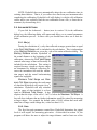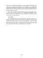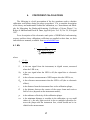
1
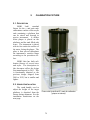
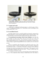
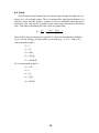
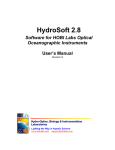
Backscattering Sensor Calibration Manual Revision P, January 2013 Hydro-Optics, Biology & Instrumentation Laboratories Lighting the Way in Aquatic Science www.hobilabs.com [email protected] Revisions Rev P, Jan 2013: Change photos to show new fixture design. Rev O, Aug 22, 2010: Formatting; revise sections 3.4.1, 3.5.3 and 3.6 to include instructions for instruments with non-flat faces (such as Series 250 HydroScat-6); correct Photflo dilution ratio in 2.4 from 1/100 to 1/200. Rev N, Oct 30, 2008: Revise recommended plaque wetting procedure (2.4), add “Final Steps” section (3.8) Rev M, May 1, 2008: Minor edits and formatting improvements. Change “target” to “plaque” in most cases. Rev L, July 3, 2006: Add note about lubrication. Rev K, June 15, 2006: Add note about Photo-Flo wetting agent and other notes about target maintenance (2.4) Rev J, July 24, 2003: Add reference to washers in fixture assembly Rev I, May 30, 2003: Add Target section (2.2) expand target maintenance section (2.4) add Coefficient Calculations section (4), include a-Beta and c-Beta in title and overview, some minor editorial changes. Rev H December 9, 2002: HydroSoft 2.6 Changes (advanced settings, section 3.9) and new recommendation for Rho in calibration (section 3.5.4). Rev G June 27, 2002: Complete revision to incorporate HydroSoft 2.5 calibration functions. Earlier revisions not tracked ii TABLE OF CONTENTS 1. OVERVIEW.......................................................................................................................................... 1 1.1. 1.2. 1.3. 1.4. 1.5. 1.6. 2. CALIBRATION FIXTURE................................................................................................................. 3 2.1. 2.2. 2.3. 2.4. 3. MU COEFFICIENTS ............................................................................................................................ 1 DARK OFFSETS ................................................................................................................................. 1 GAIN RATIOS .................................................................................................................................... 1 SEQUENCE OF PROCEDURES ............................................................................................................. 2 HYDROSOFT SOFTWARE ................................................................................................................... 2 CALIBRATION RESULTS .................................................................................................................... 2 DESCRIPTION .................................................................................................................................... 3 HANDLE INSTALLATION ................................................................................................................... 3 CALIBRATION PLAQUE ..................................................................................................................... 4 PLAQUE MAINTENANCE ................................................................................................................... 4 PROCEDURES..................................................................................................................................... 6 3.1. GENERAL PREPARATION ................................................................................................................... 6 3.1.1. Computer .................................................................................................................................. 6 3.1.2. Environment.............................................................................................................................. 6 3.1.3. Calibration Fixture and Plaque................................................................................................ 6 3.1.4. Instrument Setup ....................................................................................................................... 6 3.2. STARTUP........................................................................................................................................... 6 3.3. BASELINE CALIBRATION .................................................................................................................. 7 3.4. DARK OFFSET MEASUREMENT ......................................................................................................... 7 3.4.1. Preparation............................................................................................................................... 8 3.4.2. Data Collection......................................................................................................................... 8 3.5. MU MEASUREMENT.......................................................................................................................... 9 3.5.1. Preparation............................................................................................................................... 9 3.5.2. Setting the Channel Gains ........................................................................................................ 9 3.5.3. Measuring the Response Curves ............................................................................................ 9 3.5.4. Plaque Reflectivity .................................................................................................................. 10 3.5.5. Loading a File......................................................................................................................... 11 3.6. GAIN RATIO MEASUREMENT .......................................................................................................... 11 3.6.1. Setup ....................................................................................................................................... 11 3.6.2. Basic Procedure...................................................................................................................... 12 3.6.3. Setup and Procedure for HydroScat-6P ................................................................................. 12 3.6.4. Direction of Motion ................................................................................................................ 12 3.6.5. Continuing Procedure............................................................................................................. 13 3.7. STORING CALIBRATION RESULTS ................................................................................................... 14 3.8. FINAL STEPS ................................................................................................................................... 14 3.9. ADVANCED SETTINGS..................................................................................................................... 15 3.9.1. Mu ( ) ..................................................................................................................................... 15 3.9.2. Gain ........................................................................................................................................ 15 3.9.3. Offset....................................................................................................................................... 16 4. COEFFICIENT CALCULATIONS.................................................................................................. 17 4.1. 4.2. 4.3. 4.4. MU ................................................................................................................................................. 17 SIGMA ............................................................................................................................................ 18 DARK OFFSETS ............................................................................................................................... 19 GAINS ............................................................................................................................................. 20 iii 1. OVERVIEW HOBI Labs’ HydroScats (HydroScat-2, -4 and –6), a-Beta and c-Beta are instruments for measuring optical backscattering* in natural waters. For detailed information about these instruments, see their individual User’s Manuals, available from www.HOBILabs.com. One of their key features is the capability for a rigorous calibration that is robust enough to be performed by users in their labs or in the field. The calibration requires a fixture, described in section 2, which can be purchased from HOBI Labs. HOBI Labs’ HydroSoft software (versions 2.5 and later) guides users through the calibration to make it as straightforward as possible. The calibration has three primary parts: ratios, described below. coefficients, dark offsets, and gain 1.1. MU COEFFICIENTS Mu ( ) is the overall coefficient of sensitivity for a channel, which allows converting its normalized electronic response to absolute backscattering. This is measured by continuously moving a target plaque with known reflectivity through a range of distances in front of the sensor. The resulting curve is integrated and weighted by known geometric factors in order to calculate . 1.2. DARK OFFSETS Because of electronic factors, the instrument may produce a non-zero signal even when no scattering signal is present. These offsets (which vary from channel to channel and with gain setting) are measured by blocking the face of the instrument to prevent any light from the LEDs from entering the receivers. The dark offsets are measured out of water. The HydroScat uses the dark offset measurements internally, subtracting them in real time from the “raw” data it produces. 1.3. GAIN RATIOS HydroScats have five different gain settings. These are different levels of signal amplification, which allow automatic operation in a wide variety of conditions. The lower gain settings also make possible the method of using a highly reflective plaque for the calibration. The ratios between adjacent gain settings are * a-Beta and c-Beta also measure attenuation; this document only applies to calibration of their backscattering measurements. 1 measured by recording the signal value while a channel is set to a certain gain, changing the gain by one step, and recording the new signal value. 1.4. SEQUENCE OF PROCEDURES For a complete calibration the most convenient sequence is usually to measure the dark offsets first, since this is done outside the calibration fixture, then perform the calibration, then the gains. However it is not necessary always to perform all three steps, and their sequence is also not fixed. Because the gain ratios are the most time-consuming to measure, and also the most stable of the instrument’s characteristics, you may not wish to measure them as often. The calibration and dark offset measurements are independent of each other and can be performed by themselves at any time. The gain ratio calibration requires that the dark offsets also be measured. It is most intuitive to measure them before performing the gain ratio procedure, but it is also acceptable to reverse the sequence. HydroSoft will remind you if offsets are required to complete a gain 1.5. HYDROSOFT SOFTWARE HydroSoft (version 2.5 and later; 2.72 or later recommended) guides users through the necessary calibration procedures, collects and processes the data, and stores finished calibration results. HydroSoft is also used for routine operation of the sensors, so this document presumes your familiarity with it, and discusses the details of HydroSoft that pertain strictly to calibration. For further introduction to HydroSoft and its other features, consult the HydroSoft User’s Manual and also the manual for the instrument to be calibrated. 1.6. CALIBRATION RESULTS Finished calibration data are stored in structured text files on a computer, and also stored in each HydroScat’s internal memory. Normally the calibration stored in the instrument is considered authoritative and is downloaded from the instrument whenever HydroSoft communicates with it. However HydroSoft can also be instructed to ignore the instrument’s internal calibration and use a file instead. 2 2. CALIBRATION FIXTURE 2.1. DESCRIPTION HOBI Labs’ standard fixture for the and gain ratio calibrations consists of an acrylic tank containing a platform that can be raised and lowered in precise increments. A diffuse white plaque is placed on the platform, and the tank filled with water. The instrument is placed with its face under the surface of the water, facing the plaque. The plate is then moved throughout the instrument’s sensitive range according to the procedures below. HOBI Labs has built calibration fixtures of several sizes and styles. The descriptions in this document reflect the design first manufactured in 2013. This is functionally identical to the previous design shipped from 2001 to 2012, but is smaller and lighter. 2.2. HANDLE INSTALLATION The crank handle, used to adjust the height of the target platform, is detached from the fixture during shipment. See the installation instructions on the next page. Fixture with HydroScat-6P, ready for calibration (plaque not shown). 3 Crank handle installation: thread the handle onto the protruding rod, until about 6mm of thread protrudes above the top. Then lock it in place with the supplied nut. 2.3. CALIBRATION PLAQUE HOBI Labs’ recommended calibration plaque is a 10-inch square of Spectralon™, available from Labsphere, Inc., North Sutton, NH (www.labsphere.com) as part number SRT-99-100. 2.4. PLAQUE MAINTENANCE Spectralon plaques must be carefully handled and cleaned to maintain their calibrated reflectivity. Do not touch the calibrated surface with bare hands. Also see the maintenance instructions from Labsphere that come with the material. If you purchased your plaque directly from LabSphere, note that LabSphere plaques are held in their frames with steel screws that rust in water and may eventually stain the Spectralon. We recommend you either remove the Spectralon from the frame for use, or replace the screws with plastic or stainless steel versions. Plaques supplied through HOBI Labs have stainless steel screws that will not rust. When it is completely clean, Spectralon very effectively repels water. This means air may cling to it when it is immersed, which can seriously compromise the calibration accuracy. To determine if the plaque is properly wetted, submerge it in clean water and view the plaque from various angles. When properly wetted, it should appear uniformly white from any angle. A shiny or splotchy grey appearance indicates inadequate wetting. To avoid this it may be necessary to rinse the plaque with a wetting agent before use. We recommend a dilute solution of Kodak Photo-Flo™ 200, which is 4 available from suppliers of photographic equipment. Note that Photo-Flo is supplied in highly concentrated form and must be diluted for safe use. The best way to wet the plaque is to prepare a 1/200 dilution of Photo-Flo 200 in a spray bottle, then spray a light layer onto the plaque. Submerge it to test whether it wets properly. Continue applying more and testing as necessary. Apply only the minimum necessary, and after submerging the wetted plaque in the calibration fixture, flow additional clean water over its surface. Wetting may also be improved by letting the plaque soak in clean water for several hours after cleaning and rinsing with the wetting solution, but do not leave the plaque in water for more than a day. After removing the plaque from the calibration fixture, stand it up vertically in a sink or tank, rinse it thoroughly with clean water, and let it air-dry. 5 3. PROCEDURES 3.1. GENERAL PREPARATION 3.1.1. Computer You will need a computer with HydroSoft 2.72 or later installed, and a free RS232 serial port (or USB-serial adapter), in order to collect the calibration data. For information on setting up and using HydroSoft, see the HydroSoft User’s Manual. For the and gain calibrations you should locate the computer near the calibration fixture, in a position that allows you to view the screen and type on the keyboard while turning the crank handle on the fixture. 3.1.2. Environment Avoid bright AC lighting, and especially fluorescent lights, during the gain calibration. On high gain settings, AC lights can cause substantial excess noise. 3.1.3. Calibration Fixture and Plaque For the procedure, be sure the calibration fixture is clean and filled with clean water. The water need not be perfectly pure, but distilled, deionized or otherwise purified water will give the most accurate results. Check the plaque for cleanliness and for bubbles or any film of air clinging to its surface. A gray or shiny appearance indicates that the plaque is not completely wetted (see also section 2.4). It is preferable to fill the tank by placing the outlet of a hose near the bottom of the tank, under the water, to avoid generating bubbles. 3.1.4. Instrument Setup Be sure that the instrument either has external power supplied, or its internal batteries have enough charge to operate it during the calibration. It is best not to power the instrument from its battery charger during the calibration, as this raises the instrument’s internal temperature. Using the fast-charging circuitry in the HydroScat-6 can also cause noise in the measurements. Allow the instrument to stabilize for several minutes before beginning the calibration procedure. 3.2. STARTUP 6 In HydroSoft, connect to the instrument and verify that it is communicating properly. Except in special circumstances, you should check the Load Calibration From Instrument option in the connection dialog box. This will ensure that the revised calibration you generate contains the correct configuration information about the instrument. Select Calibrate… from the HydroScat menu, which will display the following dialog box. This contains four tabs that control the different calibration processes. 3.3. BASELINE CALIBRATION HydroSoft builds new calibration files by combining newly measured data with “baseline” data from the instrument or from a file. Data that are not revised during the calibration procedures are copied directly from the baseline to the revised calibration. Baseline data include channel names, wavelengths and other aspects of the instrument configuration, so it is very important that the baseline match the instrument being calibrated. Usually the instrument’s internal calibration is used as the baseline. When you first open the Calibrate dialog box, the calibration that is in effect in the data window from which it was opened is adopted as the baseline. Therefore it is not usually necessary to explicitly select a baseline. However you can load the baseline from a file using the From File… button, or from the instrument’s internal calibration with the From Instrument button. Whenever you select a new baseline, baseline data are immediately copied to the revised calibration, but they will not overwrite any new calibration data you have collected. Clicking the View… button will open a window in which you can browse the contents of the baseline calibration. You can leave this window open while proceeding with the calibration, in order to compare the baseline and revised data. 3.4. DARK OFFSET MEASUREMENT This procedure does not require use of the calibration fixture. It is not required for the calibration, but it is advisable to update it every time the calibration is performed. It is required whenever the gain calibration is performed. 7 3.4.1. Preparation Set the HydroScat face down on several layers of black felt or similar material. Be sure the HydroScat is on a flat surface and that its face is in contact with the covering material, so that no light can possibly travel between the windows. If the HydroScat does not have a flat face, for example a HydroScat-6P in its deployment cage, use the supplied cover that presses directly against the windows. 3.4.2. Data Collection On the Dark Offsets tab of the Calibration window, click Start. HydroSoft will proceed to measure the offsets on each of the instruments channels and gains, displaying the results in a table. It will also display the raw data in the graph window. HydroSoft calculates the standard deviation of the data while it samples the offsets and continues averaging on each gain until the maximum uncertainty falls below the value entered in the Advanced Settings dialog box (section 3.9). While sampling, it highlights the values that exceed the uncertainty goal, as shown in the illustration. Occasionally an outlying point or some disturbance to the setup may prevent the uncertainty goal from being met. In this case (or for any other reason) you can click the Undo button to back up to a previous step in the procedure. The Quit button halts the offset measurements and discards all the results. When the measurement procedure is complete, HydroSoft will ask whether you wish to save the raw data in a file. The calibration results will not be affected by whether or not you save the raw data. The saved file cannot be used to directly reproduce the results of the measurements; it is only useful for 8 trouble-shooting. 3.5. MU MEASUREMENT 3.5.1. Preparation Clean the windows, attach the mounting collar, and place the HydroScat in the calibration tank filled with clean water. To calibrate a HydroScat-4 with an integrated anti-fouling shutter, remove the shutter blade. The face of the instrument should be fully submerged and it should be level in the tank (the face of the instrument should be parallel to the plaque). Make sure there are no bubbles on the HydroScat windows, and continue to monitor the windows during the procedure to be sure that no bubbles accumulate. Also make sure that the plaque is well saturated with water, and there are no bubbles on the plaque. If bubbles begin to accumulate in either place before the calibration is complete, they must be wiped away, and the calibration must be restarted. 3.5.2. Setting the Channel Gains The first step in calibration is to determine which gain best matches each channel’s sensitivity to the calibration plaque. This requires monitoring the signals while moving the plaque through the sensor’s peak-response zone. To do this, click the Start button, then follow the on-screen instructions. 3.5.3. Measuring the Response Curves After the gains have been properly set, HydroSoft will instruct you to move the calibration plaque (“target”) to its starting position. For instruments with flat faces, move the platform until the plaque is as close as possible to the face of the instrument without actually touching it, and leave the Start Distance set to its default value of 0 cm. For a Series 250 HydroScat-6 with its deployment frame installed, set the Start Distance to 1.3 cm and move the plaque until it almost touches the frame ring. For other instruments with non-flat faces, for example a HydroScat-4 with an integrated anti-fouling shutter, measure the length of the longest protrusion for the face, and enter that value as the Start Distance. For all instruments, confirm that the Distance Step entered in the form is appropriate, normally 1.27 mm. When the target is set to its starting position, click the First Step button. HydroSoft will open a new graph in the data window, and perform some other initializations that may take a few seconds. When this process is complete, turn the crank handle one turn if your calibration fixture has 1.27 mm thread pitch (fixtures 9 manufactured before June 2002), or ½ turn if it has 2.54 mm pitch (fixtures made since June 2002), then click Next Step or press the enter key. Continue, clicking Next Step after each turn or half-turn. HydroSoft will display the evolving curves in the data window, and automatically determine when adequate data have been collected (see section 3.9.1 for details). At that time it will beep, and display a message informing you that you can either continue collecting further data, or click the Finish button to calculate the final results and transfer them to the revised calibration. 3.5.4. Plaque Reflectivity You can directly enter reflectivity values in the Rho column of the results table, either before or after collecting the data curves. The values will be recalculated each time you change Rho. For Spectralon plaques you normally use the default value of 1.10 for all channels. Note that the Rho value of 1.10 was introduced in December, 2002. The default value of reflectivity in previous HydroSoft versions was 0.98, based on irradiance reflectivity measurements provided by Labsphere. HOBI Labs revised this based on careful measurements of the radiance reflectivity, in water and at angles appropriate to the HydroScat measurement geometry. HydroSoft remembers values you enter, so previous values may still appear even after you upgrade the program. Once you enter a new value, it becomes the default. Because the previous Rho value was low, previous calibrations based on that value, and the backscattering values based on them, are also low. To compare data based on old and new rho values, you should multiply the old data by 1.12 (that is, 1.10/0.98). 10 3.5.5. Loading a File You can load curves from a previously saved file, and recalculate their values, by clicking the From File… button and selecting a suitable file. 3.6. GAIN RATIO MEASUREMENT This procedure is the most involved of the three, but because the gain values are normally extremely stable it is also not required very often. Note that the gain ratio calculations require that you also perform the dark offset calibration before saving the gain values. 3.6.1. Setup It is usually most convenient to perform this procedure in the same fixture as the calibration. However the target can be any object that can be set to stable positions, and the measurements need not be done in water. If you use water, beware of bubbles or particles that might move during the measurements. This procedure should be performed in subdued lighting, preferably with no fluorescent lights, to avoid excessive noise when measuring the higher gains. 11 3.6.2. Basic Procedure To measure the gain ratios, you move the target to a position that causes a near-peak response from one or more channels on a particular gain setting. Then, while the target remains stationary, HydroSoft measures the response to the target on the current gain, reduces the gain one step, then measures the response again. This is repeated until all gain ratios have been measured for each channel of the instrument. 3.6.3. Setup and Procedure for HydroScat-6P As explained in section 3.6.4, it is usually desirable, and sometimes essential, to measure the instrument response with the reflective target almost touching its face. However, some instrument configurations prevent this. For example, those with a built-in anti-fouling shutter, or an integrated deployment cage such as that on the HydroScat-6P. In these cases it is necessary to use a low-reflectivity (“dark”) target for close-range measurements. To do this, place the dark target on the platform of the HOBI Labs calibration fixture. Then begin the standard gain procedure, selecting the Near option as described in section 3.6.4. After the 5/4 gain ratios have been measured for all channels, remove the dark target and continue with the white platform itself as the reflective target. Dark target for gain calibration of HydroScat-6P 3.6.4. Direction of Motion When you click the Start button to begin the procedure, you will be offered the choice of starting with the target near or far from the instrument face. “Near” in this case means closer than the instrument’s peak response which is typically 5 12 to 6 cm from its face. “Far” means more than 6 cm, and on the highest gain can mean as much as 30 cm. You should normally select Near. This will keep the target in the HydroScat’s most sensitive region, requiring less motion of the target. The proximity of the target also helps shield the instrument from room lights. Note that some instruments have such high sensitivity that some of their channels will saturate even when the target is moved to its maximum distance, in which case you must use the Near option. 3.6.5. Continuing Procedure Once you have selected the direction of target motion, HydroSoft continuously monitors the signal levels from the instrument and instructs you when and in which direction to move the target. During this process it highlights the numerical signal values with colors to indicate how close they are to their ideal values. GREEN highlighting indicates values in the optimum range of 25000 to 30000. When at least one channel is in this range, HydroSoft will instruct you to stop the target, and when you acknowledge this it will proceed to measure ratios on the eligible channels. Eligible channels include those in the range from 10000 to 25000, which are shown with YELLOW highlighting. RED indicates a channel is saturated, with a value either above 30000, or at 0. In this case HydroSoft will instruct you to move the target in the appropriate direction to reduce the signal. WHITE (no highlighting) indicates a channel is either below 10000, or that it is not presently being considered for measurement regardless of its value. This can happen if the channel has already been measured on the current gain, or if hardware limitations prevent it from being measured simultaneously with some other channel. If using the “dark target” procedure described in section 3.6.3., remove the dark target after the 5/4 column is complete, as shown in the figure above. Otherwise the signal levels will not be high enough to measure the lower gains. When the gain measurement procedure is complete, HydroSoft will ask whether you wish to save the raw data in a file. As with the offset measurements, this is offered strictly as a backup in case troubleshooting is required. The calibration results will not be affected by whether or not you save the raw data. 13 3.7. STORING CALIBRATION RESULTS When you complete each calibration procedure, the corresponding check box under New Calibration Data on the Load/Store tab will become checked and enabled. This indicates that the newly-measured values have been copied into the revised calibration. You can uncheck them if you decide not to use the new data, or if you wish to compare the new and old values in the Revised Calibration window (opened by clicking on the View/Edit… button). If you leave this window open while checking or unchecking the new calibration options, you will see the values change immediately to reflect your selections. You can also compare the values side-by-side by opening both the Baseline Calibration and Revised Calibration windows. In the Revised Calibration window you can click on the lock icon to enable direct editing of most of the calibration values. Once you are satisfied with your calibration results, you can save them in the instrument’s memory, in a file, or both. When you click the To Instrument button, HydroSoft will transmit the complete calibration to the instrument, check to verify that it was correctly received, and if so ask whether you wish to save it in the instrument’s nonvolatile memory. If you choose not to, the calibration you just loaded will remain in effect until the next time the instrument is reset. A reset can be caused by a loss of power (including use of the “battery disconnect” function of battery-powered HydroScats), by an explicit reset command sent to the instrument, or by the Reset command on HydroSoft’s Instrument or HydroScat menu. If your baseline calibration was loaded from the instrument and you subsequently save a revised calibration to the instrument, the baseline retains its former values until you explicitly reload the calibration from the instrument. If you reload the calibration you will no longer be able to compare the old baseline with the new values. 3.8. FINAL STEPS When you are completely finished with the calibration, you should close the Calibration dialog box before disconnecting the instrument or putting it to sleep. During the calibration process HydroSoft changes some settings of the instrument, and it sends commands to restore these settings at the time the dialog box is closed. 14 NOTE: HydroSoft does not automatically adopt the new calibration into its existing data windows. That is, if you collect new data from your instrument after completing the calibration, HydroSoft will still display it with the old calibration values unless you explicitly load the new calibration from a file, or from the instrument (by reconnecting to it). 3.9. ADVANCED SETTINGS If you click the Advanced…. button (new in version 2.6) in the calibration dialog box, the following dialog will appear and allow you to control parameters of the calibration process. In most cases you should leave these set to their defaults. 3.9.1. Mu ( ) During the calculation of , only data collected at ranges greater than or equal to the First Valid Range will be included in the calculation. This is independent of the Starting Distance you set on the tab of the main calibration dialog. The Starting Distance informs HydroSoft of the actual distance at the beginning of the calibration, whereas the First Valid Range controls what range of data will actually be included in the calculation. This setting is required because signals at shorter ranges are dominated by multiple reflections between the instrument face and the calibration target, and the actual backscattering signals are negligible. Minimum Total Range and Maximum Tail Slope determine the total range of data that HydroSoft will require for a calculation. HydroSoft will only calculate if the range of data included is at least equal to Minimum Total Range. It also requires that the slope of the curve’s “tail” is below the Maximum Tail Slope. A low tail slope indicates that no further information would be gained by measuring at larger ranges. For example the default value of 0.001 means that each additional cm of range would change the value less than 0.1%. 3.9.2. Gain The first four gain parameters control how HydroSoft determines the signal levels it will require for measuring gain ratios. As described in section 3.6, the program will direct the user to adjust the target distance until at least one of the 15 channels is above Optimum High Signal but below Saturation Threshold. Then it will measure the gain for that channel and any others that are between Minimum High Signal and Saturation Threshold. A different Minimum High Signal is set for gain 2, because some instruments do not have enough overall gain to reach the regular threshold on that gain. When collecting gain ratio data, HydroSoft collects as many samples as are required to bring the sample uncertainty below Maximum Uncertainty. Raising this value decreases the amount of time it takes HydroSoft to measure the gain ratios, but increases the possible error. 3.9.3. Offset When measuring dark offsets, HydroSoft decides how many samples are required by calculating the statistical uncertainty of the samples it has collected, and continues until the uncertainty is below the value specified here. Some individual instruments have higher noise levels than others and therefore require more samples to achieve this uncertainty. In extreme cases the uncertainty may never fall below the threshold, in which case the threshold can be raised here. 16 4. COEFFICIENT CALCULATIONS The following is a brief presentation of the key equations used to calculate calibration coefficients during the above procedures. For a complete description of the theory and mathematics behind the calibration, see “Instruments and Methods for Measuring the Backward-Scattering Coefficient of Ocean Waters”, by Robert A Maffione and David R. Dana, Applied Optics Vol. 36, No. 24, 20 August 1997. For a description of the electronics and optics of HOBI Labs backscattering sensors, and how these calibration coefficients are applied to their data, see their individual user manuals, available from www.hobilabs.com. 4.1. MU rL m= p zmax S n ( z ) - S n ( z max ) Dz -1 ( H 2 z )) å cos(tan zmin where Sn = S - S off R - Roff S is the raw signal from the instrument, in digital counts, measured when the LED is on, Soff is the raw signal when the LED is off (the signal due to electronic offsets) R is the reference measurement of LED output when the LED is on, Roff is the reference measurement when the LED is off (due to electronic offsets), z is the distance from the instrument face to the calibration plaque, H is the distance between the centers of the source beam and receiver field of view (depends on the instrument model), rL is the radiance reflectivity of the calibration plaque. zmin is the minimum distance to consider in the calibration; at very small values of z, the only light received is due to multiple reflections between the plaque and the instrument face, which should not be included in the measurement. 17 zmax is the distance beyond which the plaque is invisible to the sensor. Note that rL differs from the irradiance reflectance normally reported for Spectralon, which is 0.99 in air. The irradiance reflectivity is the ratio of the total reflected flux to the total incident flux, and cannot have a value greater than one. On the other hand the radiance reflectance, the ratio of reflected radiance to incident irradiance, may vary as a function of angle. A perfect Lambertian reflector would have radiance reflectivity of 1 at all angles, but realistic reflectors may have values greater than 1 at some angles, indicating a specular reflection component. In this case, conservation of energy demands that that the reflectivity be less than 1 at other angles. HOBI Labs’ measurements of Spectralon reflectivity in water show that with incident irradiance at 20 degrees from normal (as for the HydroScats), its radiance reflectivity at 20 degrees reflected angle is 1.10. 4.2. SIGMA Before scattered light is measured by the backscattering sensor, it must travel from the sensor to the scattering site and back. Over that distance some light will be lost to the water’s attenuation, resulting in an underestimate of scattering. For clear waters this is insignificant, but as turbidity increases so does the underestimate of scattering. To compensate for this, calibrated backscattering values are multiplied by the function (Kbb). (Kbb) has a value of unity for very clear water, and increases as attenuation, characterized by the coefficient Kbb, increases. The response function collected in order to calculate , that is, Sn(z), is also used to derive (Kbb), which is define as follows. ¥ ( K bb ) = òW (K bbw , z )dz 0 ¥ òW (K bb , z )dz 0 where Kbbw is Kbb of the water in which the sensor was calibrated, and W ( K bbw , z ) = S n ( z ) - S n ( z max ) cos(tan -1 ( H 2 z )) It can also be shown that having measured W (Kbbw, z) during the calibration procedure, one can then calculate, for any Kbb, W ( K bb , z ) = W ( K bbw , z ) exp(( K bbw - K bb )(rs + rr ) where 18 rs is the distance along a line from the center of the source beam to the center of the scattering site, rr is the distance along the return path to the receiver. Using these relationships, HydroSoft can then calculate z max ( K bb ) = åW ( K bbw , z ) Dz z min z max åW ( K bb , z )Dz z min However to enable a much more efficient calculation of ( K bb ) during processing of in-situ data, as well as to minimize the amount of information that must be contained in an instrument’s calibration file, we desire to simplify the above expression. Because of the exponential relationship between W ( K bbw , z ) and W ( K bb , z ) , ( K bb ) can be closely approximated by ( K bb ) @ k 0 exp( K bb k exp ) where k exp = ln ( K bbw + 3) K bbw + 3 and k 0 = exp( - k exp K bbw ) For these coefficients, HydroSoft calculates Kbb by assuming the calibration water has absorption equal to that of pure water, and scattering equal to twice that of pure water. While these are obviously crude assumptions, their effect on the outcome of the computation is very small, unless very poor-quality water is used during the calibration. The value of 3 used in the above expression for kexp was determined empirically to provide very accurate fitting of ( K bb ) for Kbb values from 0 to 10. 4.3. DARK OFFSETS S D (g ) is the residual signal measured on gain g (where g designates one of five possible gain settings), when there is no actual backscattering signal present. It is calculated (for every gain on every channel) by S D ( g ) = S - S 0 (see the variable definitions above). 19 4.4. GAINS Each backscattering channel has five discrete gain settings that adjust its sensitivity over a five decade range. They are measured by adjusting the distance to a reflective target until the sensor’s response is near its maximum; then the gain is reduced by one step and the response to the same target measured on the lower gain. This allows calculating the ratio of the two gains from Rg = Gg G g -1 = S(g) - SD (g) . S ( g - 1) - S D ( g - 1) Once all four ratios are known, the specific G values are determined by defining Gg as 1 for the setting g in effect when is measured (g = 1 or 2). That is, if was measured on gain 1, G1 = 1 G2 = R2 G3 = R2 R3 G4 = R2 R3 R4 G5 = R2R3R4R5 If was measured on gain 2, G1 = 1/R2 G2 = 1 G3 = R3 G4 = R3 R4 G5 = R3R4R5. 20