1
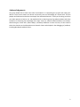
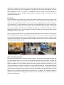
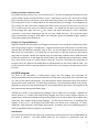
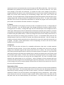
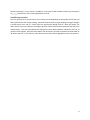
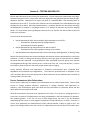
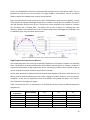
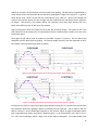
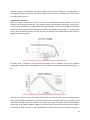
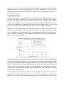
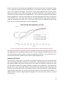
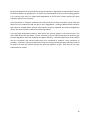
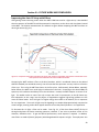
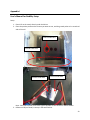
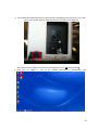
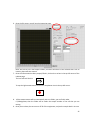
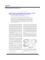
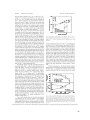
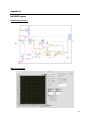
Improving the Stability of Amorphous Silicon Solar Cells ECpE Senior Design May12-09 Final Report 4/26/2012 Iowa State University Advisor- Dr. Vikram Dalal Team: Anthony Arrett Wei Chen William Elliott David Rincon Brian Modtland 0 Table of Contents Section I – Design and Implementation .................................................................... 3 Project Progression ..................................................................................................... 3 Standards ..................................................................................................................... 3 Hardware ..................................................................................................................... 5 LabVIEW Program ........................................................................................................ 6 Section II – Testing and Results ................................................................................ 9 Device Parameters after Fabrication .......................................................................... 9 High Temperature Anneal of Devices ................................................................... 11 High Temperature Deposition of Devices............................................................. 12 Comparison of Devices ......................................................................................... 14 Degradation Results .................................................................................................. 15 Defect Density ........................................................................................................... 16 Summary of Results .................................................................................................. 18 Section III – Future Work and Conclusion ............................................................... 20 Improving the Stability Setup .................................................................................... 20 Future Use ................................................................................................................. 22 Conclusion ................................................................................................................. 22 Appendix .............................................................................................................. 23 I. User’s Manual for Stability Setup ....................................................................... 23 II. NREL Journal Article ........................................................................................... 26 III. LabVIEW Program ............................................................................................... 29 1 Awknowledgements Our group would like to thank those who have helped us in completing this project and making our devices. This of course means our advisor and primary source of knowledge, Dr. Vikram Dalal. The two people who fabricated our devices were Keqin Han and Sambit Pattnaik. Thank you for taking time from your other projects to help us out. We would also like to thank a group of graduate students who have assisted us in enhancing our knowledge of the topic: John Carr, Mehran Samiee Esfahani, Siva Konduri, Shantan Kajjam, Pranav Joshi, Robert Mayer, and Randy Gebhardt. Last but not least, we also need to thank the scientists at the Microelectronics Research Center who helped in the debugging of problems, including Max Noack and Ruth Shinar. 2 SECTION I – DESIGN AND IMPLEMENTATION Project Progression As noted in the project plan, the project changed dramatically throughout the two semesters. Originally the plan was to be strictly research and analysis. The first several months of the project required extensive research into the physics of amorphous Silicon solar cells. In particular, Paul Stradins’ (et al.) article, Anneal treatment to reduce the create rate of light-induced metastable defects in device-quality hydrogenated amorphous silicon, shown in Appendix II, was the main focus of the research. Then a plan was developed as to how testing was to proceed. As time progressed the need for better equipment in the Microelectronic Research Center became apparent. The project then evolved into developing an automated I-V measurement setup. This required research into different types of hardware, and learning how to code with specific software. One of the main objectives became to build a setup that would last for years. This meant choosing hardware that was reliable and accurate. The software was written in a language that could easily be modified, so future users could change what was necessary. The chosen programming language was Nation Instrument’s LabVIEW. After the hardware was set up, measurements were started, and the system was calibrated. In the end, good research was performed with important results, and a setup was created that will help Iowa State University researchers better understand solar cells for years to come. Standards AM 1.5 Solar Spectrum Since the project is primarily research based, our standards had to be in line with recent scientific studies. This includes light soaking under a standard measurable light spectrum. This was resolved by using an ABET 10500 Solar Simulator. Solar cells are extremely sensitive to the wavelength of the photon incident on it so it is important that the light source match the spectrum of the sun. If a photon has a wavelength that is too large for the solar cell, it will not produce electron hole pairs, and thus will not produce energy, regardless of the intensity of the light. The main research standard is the AM1.5G solar standard. This is a standard developed by the photovoltaic industry, government research and development laboratories, and the American Society for Testing and Materials. The ASTM defines two solar spectra, AM0 and AM1.5 (with two variations). The AM stands for ‘air mass’ and the 0 and 1.5 are based on the number of atmospheres the light has to pass through. So the AM0 is based on the solar irradiance as seen in space. The AM1.5G is based off the spectrum as seen from the ground at a solar zenith angle of 48.2°. It is a reasonable average of the average irradiance from the sun that strikes the contenential United States of America over a year. This may seem incorrect, but since the United States receives sunlight at an angle, the light goes through more than atmosphere. The solar industry uses AM1.5G almost exclusively for all standardized testing of terrestrial solar panels. The atmosphere will affect the sunlight by absorbing certain wavelengths. Some wavelengths are absorbed completely and some will have a lower spectral irradiance. Figure 1-1 below shows the AM0 and AM1.5 spectrums. Notice how UV light is absorbed by ozone and IR radiation by water vapor. 3 Figure 1-1. AM0 and AM1.5G solar spectrums. The red plot is the goal of our light source. Amorphous silicon has a bandgap of approximately 1.7eV, which means that only light of wavelength shorter than 729nm will produce energy, although due to defects larger wavelengths are still absorbed. The ABET Solar Simulator was made to duplicate the AM1.5G spectrum as closely as possible using filters to simulate atmosphere. It is a big step up for the MRC over the Xenon lamp that was used previously. This leads to a more accurate measurement of the solar cell’s efficiency in real world applications. IEEE-488 Standard When we were designing our system to complete the automated I-V measurements, a way to communicate with the measurement equipment was needed. Mostly, communication with the Keithley 236 Source/Measure Unit (SMU) was desired. The standard communication bus for this kind of application is IEEE-488. The IEEE-488 standard allows remote control of the measurement equipment with the LabVIEW program that was written to perform the I-V testing of our solar cell devices. IEEE-488 is a short-range digital communications bus specification. It was developed specifically to control automated test equipment, such as our Keithley 236. The IEEE-488 standard is normally recognized as the GPIB standard or General Purpose Interface Bus. In order for our Dell PC to communicate with the Keithley device via IEEE-488, the use of a USB-GPIB connector was required. The Keithley 236 was selected for its specifications, but also because it was already outfitted with an IEEE488 input, so no additional converter was necessary. By selecting an address for each device being controlled, in our case two devices, each could be controlled independently by LabVIEW. Figure 1-2. IEEE-488 Female Connector (http://en.wikipedia.org/wiki/File:IEEE-448.svg). 4 IEEE-488 is still widely used today, but has been superseded by newer interface bus standards that are much faster and allow for more configurations. Fortunately for this project, IEEE-488 was sufficient, keeping equipment costs to a minimum. IEEE-488 has been very useful to the improvement of automated solutions and has provided a widely supported, reliable solution for communication with measurement equipment. Hardware For the automated I-V measurements, a system was need that could expose the solar cell to light, while doing a current vs. voltage sweep at given time intervals. In order for this to be accomplished, it was necessary to purchase a solar simulator, a source-measure unit, a digital ampmeter, and a computer to run the software. The final components chosen were an ABET 10500 short-arc solar simulator with AM1.5 filters, a Keithley 236 source-measure unit, and a Dell OptiPlex desktop computer. The Keithley 236 is the most important piece of the setup besides the light source and allows two probes to source voltage and measure current. This is important to reduce the number of contacts made and to prevent shadowing loss from excess probes. The plan originally called for the use of a Keithley 485 picoamp meter as the reference cell multimeter, but for simplicity and economy a Keithley 197A was used. The reference cell current measurement did not require the picoamp resolution that the 485 provided so money was saved using a Keithley 197A already located at the MRC. The desktop required a GPIB to USB converter to allow it to communicate with both the Keithley 236 and 197A. Figure 1-3. Completed Setup for Automated Stability Testing. ABET 10500 Solar Simulator The center of the automated I-V system is the solar simulator. This is used to soak the device under light for a prolonged period of time. This is done so the change in efficiency can be measured. The ABET was bought over other simulators because it can produce a solar spectrum that meets the AM1.5 solar spectrum standards at a cost of $4500 compared to other simulators costing over $20,000. This is the universal standard that is used to characterize a solar cell as described above. It was discovered during testing that the solar simulator is a bit heavy in the ultra-violet light, so a silicon carbide filter is used to match the spectrum closer to the desired solar spectrum. This simulator was used over a Xenon arc lamp because of the complexities required with the Xenon lamp. In addition, this simulator replaces a stability setup which uses ELH halogen lamps which have a rated lifespan of only 40 hours, much too short for our experiments. 5 Keithley 236 Source-Measure Unit The Keithley 236 was chosen as the source-measure unit. This piece of equipment would do all of the current-voltage sweeps and measurements. It was a requirement that the unit could source voltage while measuring current, and source current while measuring voltage. This allows the software to set the starting point for the I-V sweep based on the measured open-circuit voltage. At the beginning of every sweep, the unit would source voltage and measure current to find the short circuit current, and then it would source zero current and measure voltage. This would find the open circuit voltage. A starting voltage 20% larger than the VOC was chosen, and swept backwards to -0.5V in adjustable increments. It was also a requirement that the unit have a GPIB connector. This connection would allow communication through a GPIB cable to the computer, where the LabVIEW program would be running the sweeps and measurements. Keithley 197 Digital Multimeter Originally a Keithley 485 was chosen as the digital current meter, but it was quickly realized that it didn’t have a large enough range for our application. A digital multimeter that could measure up to 10mA was required while the 485 had a maximum range of 2mA. An unused Keithley 197 was discovered at the MRC that fit this requirement. This meter was not as accurate as a 485, but accuracy in the picoamp range was not required. Besides the required range, the multimeter needed to have a GPIB connector just like the Keithley 236. At the beginning of every sweep, the LabVIEW program would take a reading of the short-circuit current of a nearby reference solar cell. That way, if there were any fluctuations in the light source, the reference cell would detect it and adjustments to the results could be made. This lets the researcher know if it was degradation in the solar cell or just a change in the light spectrum from the lamp. LabVIEW Program The heart of our automated I-V measurement system was the program that controlled the measurement devices which returned an extensive set of data over a long period of time, 100 hours per run. During each stability measurement, over 200 itereations with three different delay times between measurements were conducted. The time delay varied from 1 minute between sweeps to 30 minutes depending on how much total time had elapsed. Initial measurements were taken closer together with later measurements being spread farther apart. LabVIEW was chosen as the programming language used to implement our program. LabVIEW was chosen because it is a widely used programming language and it has a rather simplistic approach to programming. Graphical block diagram programming allows a user to see the flow of the program much more easily than standard programming languages. This also allows future users to manipulate the program as they see fit. The program was broken down into several parts: initialization, I-V sweep, calculations, data exportation, and variable loop iteration. A symbolic view of the LabVIEW program is shown in Appendix III with the program’s user interface. Initialization The first thing that had to be done before any of the program would work was to set the GPIB address of the device in software. The GPIB address allows for the program to communicate with the 6 measurement device and automatically control through the IEEE-488 standard bus. Once the correct GPIB address was specified, the initial measurements of the solar cell device could start. First, open circuit voltage of the device was measured. To measure the open circuit voltage of the device a programming block was written to turn the Keithley 236 into source current/ measure voltage state and supply zero current while measuring the corresponding voltage. Next, short circuit current was measured. This was completed with a programming block that did the opposite of what the open circuit voltage program did, naming sourcing zero voltage while measuring current. The open circuit voltage and short circuit current are important measurements to initialize the program and are also key data points used in the calculations that were used later in the program. I-V Sweep After the initialization of the program, the next part was to complete the current vs. voltage sweep of the solar cell device. First, we used the open circuit voltage calculated in the earlier stage to find our starting point for the sweep. A voltage 20% larger than the calculated open circuit voltage was used in order to get a better picture of the IV characteristics of the device, especially series resistance. Once the starting point was specified, the step voltage was determined based on the stop voltage of -0.5V and the increment value given (default 10mV). A small step voltage was chosen for the sweep, around 10 mV, to allow more data points per sweep, giving a smoother I-V curve. An intermediate delay time was also selected between each step to allow for accurate, but efficient data collection. Once the sweep was complete, the dynamic data measured was then converted into arrays, which were then entered into an X-Y graph. This gave a visual representation of the corresponding I-V curve to the user for instant feedback of solar cell performance Calculations In order to test the solar cell device for acceptable performance, there were a couple important calculations that were desired. Three of these calculations, max power point, max current, and max voltage, were calculated using the data arrays formed from the I-V sweep. The current and voltage arrays were passed through functions to look for the maximum points in the data set. Once these two values were found the max power point could be found. With the max power point, the fill factor could be calculated a given sweep. Fill factor was calculated by comparing the open circuit voltage and the short circuit current versus the max current and max voltage points. The ratio of maximum power divided by the optimal power (ISC*VOC) is fill factor. Lastly a calculation of shunt resistance and series resistance was done using the IV curve and finding the slope of key data points. The inverse of the slope at zero voltage is the shunt resistance (ideally infinite) while the inverse of the slope at zero current is the series resistance (ideally zero). Exportation of data Once all the data was successfully measured and calculated, the data was stored in Excel spreadsheets for further data analysis. This was automatically done since there were over 200 sweeps and over 50 data points per sweep, meaning a lot of data to store manually. A function in LabVIEW was found that allowed the creation of our own file directory at the beginning of every measurement. With a standalone directory for each solar cell device sample, another function would send the raw data into files and place them into the created directory for each device. In this way each sample had its own 7 directory with each I-V curve stored. In addition, a summary file was created to allow easy comparison of ISC, VOC, and fill factor over time as degradation occurred. Variable loop iteration The main purpose of our project was to find a solution to the degradation of amorphous silicon solar cell device performance due to light soaking. Research shows that early in light soaking, the largest changes in performance occur and at a certain point the performance would level off. With this known, the desire was to have more sweeps at the beginning of the measurement and less sweeps at the end of the measurement. This was accomplished by having one minute delays between sweeps for the first 20 minutes of the program, then 10 minutes delays until 90 minutes, and the last sweeps would be taken at 30 minute intervals. In this manner, more data points are taken where degradation occurs the quickest. 8 Section II – TESTING AND RESULTS Devices were fabricated as part of two main experiments. The first experiment involved the use of hightemperature anneal of the P-I layers after they were deposited using plasma-enhanced chemical vapor deposition (PECVD). Deposition of all layers was done at a standard 400°C, with annealing done at temperatures up to 425°C. The second set of devices were not annealed, but instead deposited at high temperatures up to 450°C. With the annealed devices, a secondary process was also tested, that being rehydrogenation of samples in a hydrogen plasma in an attempt to passivate any left-over dangling bonds. For some devices, boron grading was also used to try to improve the internal electric field and assist carrier collection. An overview of the experiments: Devices deposited at 400°C and annealed at high temperatures up to 425°C o Some devices rehydrogentated in hydrogen plasma o Some devices with Boron gradient Devices deposited at high temperatures from 400°C to 450°C o Some devices with a Boron gradient starting at N-I interface Standard devices were deposited at 300°C with no annealing, rehydrogenation, or Boron grading Results of these experiments are summarized below with the best devices represented from each group of devices. Current vs. Voltage and quantum efficiency curves are given for some devices to establish the trends that were observed. Once good devices were established from each group, these samples were degraded under light with intensity that is 2 times that of the sun. Every few minutes, I-V curves were taken to observe how the main solar cell parameters were changing. Finally, quantum efficiency and capacitance vs. frequency measurements were conducted postdegradation and compared to pre-degradation. The results are presented with an emphasis on the most successful devices from each experiment to draw conclusions on the methods most successful at creating stable a-Si:H solar cells. Device Parameters after Fabrication Once a device is fabricated, a standard set of measurements were taken of each device. These include current vs. voltage, quantum efficiency, capacitance vs. voltage, thickness, and capacitance vs. frequency. Each measurement gives more detail into the performance of a particular device and also helps tweak the next sample to be made. Of these measurements, three are most important for this study. First, current vs. voltage gives the I-V curve that is common of all photovoltaics, that being a photodiode in the fourth quadrant of operation, thus producing power. In PV, the I-V curve is often flipped across the x-axis in the first quadrant understanding that current is really negative compared to forward direction in a diode. From the I-V curves, three parameters are obtained which quickly indicate whether a device is good or bad. The open-circuit voltage indicates how well carriers are separated by the internal electric field under open9 circuit conditions. Short-circuit conditions give the maximum current that the device will provide to a load and indicates how many carriers are successfully collected. Finally, fill factor is a property of solar cells that indicates the “squareness” of the I-V curve. The higher the fill factor, the more power that is generated compared to the power of ISC times VOC. Fill factor can never by 100%, but most commercial cells have a fill factor greater than 70% with the best cells over 80%. Due to the difficulties with a-Si, the goal of these experiments is over 60% after degradation. Figure 2-1 gives a graphical overview of these parameters. Figure 2-1. Solar cell parameters relating to I-V and power The second most important measurement is quantum efficiency (QE). The purpose of QE is to indicate how well a cell absorbs a given wavelength and then coverts that into collected current. Ideally, any solar cell would collect every carrier that is generated by light, but that is not possible due to recombination through many mechanisms. Normally, QE is done under short circuit conditions to see where ISC is coming from and to compare between devices whether more carriers generated by a given wavelength are better collected. Under a small forward bias (0.5V), QE is repeated and the ratio of short-circuit to bias conditions is plotted. This QE ratio indicates good devices if the ratio is near 1 as no matter the bias, carriers are collected. If the QE varies from 1.0, then problems exist in the device, most notably poor collection due to recombination of minority carriers. The final measurement of importance is capacitance versus frequency. By measuring capacitance in the device for frequencies ranging from 20Hz to 200kHz, a plot of the defect densities versus energy from the conduction band can be made. This is very useful to this study, as the hope is to detect changes in the defects after light exposure to see if an explanation can be established. C-f measurements are time consuming so they were only performed on devices that were degraded, both before and after light exposure. With an explanation of the main measurements given, the results are provided below with a discussion of the findings. The results are broken into two sections based on the two main experiments, one for high temperature anneal and one for high temperature growth. 10 High Temperature Anneal of Devices For the anneal experiment, devices were deposited at 400°C and then annealed once the intrinsic layer was completed, prior to the P layer. Annealing was done in the same reactor as deposition in a nitrogen atmosphere at 400°C and 425°C. Anneal temperatures were tested as low as 350°C and as high as 450°C but neither produced devices worth reporting. During growth, some samples were given a gradient of Boron doping from 0ppm to 28ppm starting at the N-I interface to improve the internal electric field in the area where most recombination of holes occurs, resulting in lost current. While annealing the N-I layer, some samples were exposed to a hydrogen plasma to rehydrogenate the dangling bonds created during the high-temperature anneal. Hydrogen is a small enough atom to diffuse though the a-Si lattice. When it finds a dangling bond with an electron available for covalent bonding, the hydrogen “sticks” and passivates the bond so it doesn’t act as a recombination center. Table 2-1 summarizes the I-V characteristics of the different anneal temperatures. Anneal Temp. Rehydrogenation 400°C 425°C 400°C 425°C 400°C 425°C Standard No No No No Yes Yes - Boron Grading No No Yes Yes Yes Yes - VOC ISC FF 0.866V 0.861V 0.871V 0.842V 0.868V 0.855V 0.822V 1.23mA 1.23mA 1.32mA 1.32mA 1.12mA 1.09mA 1.29mA 58.6% 60.3% 61.6% 59.3% 61.2% 57.8% 64.5% Table 2-1. I-V Characteristics of Solar Cells created Under Different High Temperature Anneal Conditions. From the table, the VOC values are all between 0.8V and 0.9V. Short-circuit currents range from 1.09mA for the 425°C annealed device with rehydrogenation and boron grading to 1.32mA for the devices with boron grading but no rehydrogenation. The short-circuit currents are even larger than the standard device which indicates greater number of collected carriers. Comparing fill factor values, none of the devices surpassed the standard device value of over 64%. The largest FF measured for the annealed devices was 61.6% for the 400°C with only the boron grading. Overall, the best device made from the annealed experiments was sample 2-16044, at 400°C anneal and a high VOC=0.871V and ISC=1.32mA. Overall trends show that including rehydrogenation is not beneficial to the devices. Current descreases and fill factors are not improved as desired. This indicates a process that does not work to passivate the dangling bonds in order to reduce recombination. Boron grading is definitely advantages. A boron graded devices, including those not shown, have been current and FF on average than devices without. Thus, adding ppm amounts of boron to the intrinsic layer is worth the effort in order to improve devices. 11 Finally, the standard device is hard to outcompete when looking at initial I-V parameters alone. This is a good control recipe for a-Si:H as it provides a very high standard. Unfortunately, most of our devices failed to surpass this standard when using the anneal method. Figure 2-2 below shows the QE results for the 425°C annealed device with only boron grading. Looking at the QE plot, the optimal wavelength of operation is at 540nm, exactly where it should be since that is near the maximum intensity from the sun. The QE ratio is more important in this context as it explains why this device has a FF below 60%. Past 650nm, the QE ratio is above 1.2, indicating poor hole collection. Before holes can diffuse from the N-I interface where these wavelengths are absorbed to the P-I depletion region, they recombine with electrons. Figure 2-2. Normalized QE and QE ratio of 400°C annealed device with TMB grading. High Temperature Deposition of Devices The second experiment was to use high temperature deposition of a-Si devices instead of just annealing them. The benefit is an uninterrupted process which reduces interface defects. In addition, the desire is to gain the same benefit as high temperature anneal, that being less defects when exposed to light as more Si-Si bonds are formed instead of easily broken Si-H bonds. Devices were deposited via plasma-enhanced chemical vapor deposition (PECVD) as with all of our a-Si devices, with the ambient temperature in the reactor ranging from 400°C to 450°C in more recent tests. In addition, as with the first experiment, some of the devices were graded with boron in the intrinsic layer of the device from 0ppm to 32ppm. Table 2-2 summarizes the I-V characteristics of the different devices created at different deposition temperatures. Growth Temperature 400°C 425°C 400°C 425°C 450°C Standard Boron Grading VOC ISC FF No No Yes Yes Yes - 0.907V 0.854V 0.884V 0.877V 0.866V 0.822V 1.00mA 1.08mA 1.07mA 1.13mA 1.15mA 1.29mA 54.7% 56.7% 63.1% 63.8% 66.9% 64.5% Table 2-2. I-V Characteristics of Solar Cells created Under Different High Temperature Deposition Conditions 12 Looking at the table, the best devices were those with boron grading. The best device created based on initial measurements was the 450°C device with boron grading with a large FF of nearly 67%. In general, these devices have a lower current than the anneal devices from Table 2-1. Open-circuit voltages are similar to the previous devices, but are all larger than the standard device, indicating a better separation of charges. Unfortunately, the standard device still competes heavily with these devices and has a better initial efficiency than all but one of the samples. Higher temperatures seem to increase FF and current, but decreases voltage. The reason for this is not well understood at the moment, but if recombination centers are decreasing in number, then this result would make sense. Once again the QE and QE ratio of samples are provided in Figures 2-3 and 2-4. The first device was deposited at 425°C without boron grading. The second sample (2-16127) was also deposited at 425°C but includes a boron gradient from 0ppm to 32ppm. Figure 2-3. Normalized QE and QE ratio for device grown at 425°C without boron grading. Figure 2-4. Normalized QE and QE ratio for device grown at 425°C with boron grading. The QE plots are hard to compare (see Figure below with discussion), but it is obvious from the QE ratios that the device with boron grading is better at collecting carriers in general. The QE ratio for the first device is above 1.2 for all wavelengths especially in the sensitive region of longer wavelengths where light is absorbed much farther from the P-I depletion region. In the second device, the ratio is near 1.1 to 1.2 for most wavelengths which a larger ratio at the longer wavelengths. This improved QE result 13 indicates a higher current density in the device (larger ISC) without even taking an I-V measurement. It also indicates a device with a better FF because fewer carriers are lost to recombination. These results are confirmed by Table 2-2. Comparison of Devices Figure 2-5 shows a comparison of the I-V curves for the three devices compared above. The curve confirms the trends discussed above. The standard sample and annealed sample have a larger shortcircuit current compared to the high-temperature growth devices. Open-circuit voltages for all devices are about the same, but the 425°C growth device with boron grading has the largest VOC. Looking at the curves, all have decent fill factors, but the best two are obviously the standard device and the 425°C deposition sample with boron. Figure 2-5. Comparison of I-V characteristic of 3 samples from each experiment. To better show a comparison of how these three devices fair at producing current from different wavelengths of light, the normalized QE curves for each device is compared on the same plot (Figure 26). Figure 2-6. Normalized QE comparison between devices from both experiments. From Fig. 2-6, notice first that the standard device collects far more current in the UV and blue portion of the spectrum (450nm and below). All devices perform best in the green part of the spectrum as they should with the peak of the sun’s radiation occurring at that range. The 425°C anneal device performs much better in the range of 600nm to 800nm, producing more current (1.32mA) than the other devices as indicated in Table 2-1 and 2-2. The 425°C deposition devices have nearly the same QE, resulting in 14 similar ISC values. In summary, the QE plot confirms the measurements made above and indicates the wavelengths which are not being collected by the cells, namely above 650nm. The 425°C anneal treatment produces the device with the best QE, but further tests show significant degradation as is shown in the next section. Degradation Results Once the best devices of a recipe were identified, these samples were degraded under light of two times the intensity of sunlight for 60+ hours. The setup was calibrated for 2x sunlight using a standard crystalline solar cell with a known short-circuit current under 1x sun. By using that working standard, the setup was calibrated for 1x and 2x measurements by moving the light source until the short-circuit current of the standard cell was producing the known 1x and 2x currents. With c-Si this method produces acceptable error compares to absolute 1x light according to the AM1.5G standard. Degradation as shown by the Staebler-Wronski effect is mostly due to a decline in the fill factor of cells as they are exposed to light. ISC and VOC also decline over time, but not to the same extent as FF does. Thus, the parameter of importance when trying to improve degradation of these cells was the fill factor over time. Figure 2-7 shows how fill factor degrades in the three samples which are all heated to 425°C during part or all of their fabrication. Figure 2-7. Fill factor degradation over time while exposed to 2x sunlight intensity. The standard sample is included for comparison. With exposure to 2x light, it degrades from a FF of 65% to one of around 57% after 60 hours. Figure 2-8 shows a normalization of this degradation for ease of comparison, showing the standard cell degrades by over 14% from start to finish. The 425°C anneal device, which showed promise based on the QE plot, also degrades by this same percentage. Comparing to other cells which were degraded, this is one of the most stable devices created under the high-temp anneal method. This indicates that using high-temp anneal after the P-I layer is deposited is not useful at producing more stable a-Si cells. The high-temperature growth devices do show some promise though. Looking at Figs. 2-7 and 2-8, the devices grown at 425°C degrade by less than 10% in fill factor. Even better, after 60 hours of light soaking at 2x sun intensity, the device with boron grading has a fill factor equal to 59% whereas the 15 standard device is at 56% at 50 hours, allowing for a higher efficiency. Further work needs to be done on this method, but currently results show less degradation under high-temp growth of devices. Figure 2-8. Normalized FF degradation under 2x sunlight light exposure. The plots above give the degradation of FF, but ultimately the desire is stability in power conversion efficiency over time. Figure 2-9 gives a normalized degradation of power efficiency for the hightemperature growth devices, which includes degradation to VOC and ISC. Looking at the plot, it is no longer obvious that high-temp deposition is a way to improve stability. What gains are made in FF are lost in degradation of VOC and ISC. Fortunately, these parameters can be worked on with tweaks to the recipes. But compared to the anneal method in which efficiency degraded by 25% over 60 hours, using high-temp growth produces devices which are as stable or marginally better than the standard recipe. Figure 2-9. Normalized Power Conversion Efficiency degradation under 2x light exposure. Defect Density To try and establish the mechanism for degradation of the I-V characteristics of the cell, capacitance versus frequency measurements were taken before and after light exposure. This measurement, done with frequencies between 20Hz and 200kHz, allows a plot of the defect density as a function of energy to be formed. In a-Si, it is known that defects occur in the forbidden band gap because of defects in the 16 lattice compared to c-Si material. In addition, defect states occur as a result of impurities which fabricating the devices and from dangling bonds that form as a result of broken bonds in the lattice. Capacitance vs. frequency measurements are thus used to see if a correlation can be made between the degradation of the I-V characteristics of the device and the relative changes in the defects in the material. Figure 2-10 gives the defect density of the 425°C growth device (no boron grading) before and after light exposure. The measurements confirm the explanation of a-Si degradation; that the number of defects should increase with exposure to light if the device is performing worse. The plot also shows that in this device, there are more defects in the mid-gap of the device compared to 0.4eV below the conduction band, and that this difference increases with exposure to light. But his device only degraded by 10% in FF, saying that the changes in the mid-gap states might not be playing a big role in the degradation of FF. Figure 2-10. Defect density in 425°C growth sample (no boron grading) before and after light soaking. Next, defects are looked at for the device which was grown at high-temperature and includes boron grading. In the mid-gap of the band gap, defects increase with light exposure, but near the band edge the defects actually decrease. The reason for this decrease is unknown, but further tests might allow further insight. Boron as a dopant is p-type so its effect would be on the valence side of the gap and is not shown in this plot. Either way, this device degrades at almost the same amount as the previous device, meaning this weird behavior might also not matter when explaining degradation. Figure 2-11. Defect density in 425°C growth sample with boron grading before and after light soaking. 17 Finally, a comparison of the defects after degradation for the same three devices is presented in Figure 2-12. Looking at the graph, the 425°C anneal device has more defects after light exposure, especially closer to the conduction band edge. This may be why this device degraded more than the others. Looking at the defects near 0.45eV on the graph, the amount of defects at those energies seems to correlate inversely with the devices that degraded more. Thus, devices with larger defects around these energies degrade more. Given the small sample size measured and displayed in the plot, this conclusion is just a trend to note. Once again, further analysis and measurement of a larger sample of devices is needed to see whether this is true or not. Since a given defect cannot be attributed to these energy levels, there is no reason to believe this is a cause of degradation. Figure 2-12. Comparison of post-degradation defect densities in samples of different fabrication conditions. One thing that seems to be clear from the plot is that defect densities near mid-gap are nearly the same after light exposure for considerable amounts of time. Thus, the mid-gap states that Stradins et al. were concerned with do not seem to matter in relation to degradation of fill factor. This may be why there is a disconnection between the NREL research and the research displayed here. Summary of Results To summarize the results given in this section, two methods of creating a-Si:H solar cells was looked at with various design parameters changed in each experiments. High temperature anneal of the P-I layer after growth at 400To summarize the results given in this section, two methods of creating a-Si:H solar cells was looked at with various design parameters changed in each experiments. High temperature anneal of the P-I layer after growth at 400°C creates devices which have high short-circuit current, but fill factors mostly below 60% unless boron grading is used to increase hole collection. Rehydrogenation using hydrogen plasma does not produce devices which perform better than devices without. In addition, devices annealed at high-temperature degrade more than the devices made by a standard (control) recipe. 18 By doing all deposition of the entire device at high temperatures, degradation is improved while samples still have parameters of a good device. Fill factors are improved with the use of a boron doping gradient in the intrinsic layer from 0 to 32ppm while degradation of the fill factor remains around 10% when exposed to light of 2x sun intensity. From capacitance vs. frequency measurements it was shown that no clear correlations can be made, but defects near the conduction band may play a role in degradation. Looking at defects before and after light exposure, mid-gap defects increase after exposure to light as expected, but based on degradation results, they seem to make no difference concerning stability. In the end, high temperature growth at about 425°C with a boron gradient in the intrinsic layer is the most stable device that was tested. Further tests hope to find an ideal temperature for growth to get the best degradation while still producing the highest efficiency. Extended experiments on the defects near the conduction and valence bands need to be conducted to establish a true connection to instability. Moreover, material measurements using microscopy and spectroscopy techniques need to be used to see how the material changes over time with exposure to light. Only then can the most stable device be created. 19 Section III – FUTURE WORK AND CONCLUSION Improving the Auto-IV Setup with Filters After getting some interesting results when the ABET 10500 was used as a light source, it was decided that the spectrum of the ABET should be measured in comparison to the other solar simulators located at the MRC. The relative measurements of irradiance are given below comparing the ABET simulator to other light sources (Fig. 3-1). Figure 3-1. Comparison of the Spectral Irradiance of various solar simulators at the MRC. Note that the Oriel simulator is the most expensive and is calibrated to be closest to AM1.5G standard. Comparing the ABET without a filter to the Oriel simulator, which is considered closest to the desired AM1.5G standard (see standards section), one will note that the spectrums are very similar at a fraction of the cost. This is why the ABET was chosen in the first place. Unfortunately, below 400nm, especially below 350nm, the ABET has a much higher irradiance than the Oriel. Comparing to the desired AM1.5G spectrum, the irradiance should drop off as the Oriel does. Instead, the ABET outputs an excess of UV light. This would not be an issue if the only concern was initial I-V parameters, as the QE shows very little absorption in this range, but the physics of degradation suggests high-energy photons are the cause of broken bonds. Since UV light is of higher energy than visible or IR radiation, this is important for our experiment. Too much UV light may be degrading our samples disproportionately compared to actual sunlight, meaning results which appear worse than how they would perform in real application. To eliminate this UV light, a filter can be made. From Fig. 3-1, a filter that allows 10-20% of the UV through and almost the entire remaining spectrum is desired. If one tries to purchase a filter of this character, difficulties arise. To get the desired performance, much expense is required. In addition, most filters are made of plastic (polymers) which degrade which exposure to light. These polymers also 20 break down under high-energy light so eventually a plastic filter would need to be replaced. Besides the cost of replacing, during a single 100 hour run, results may be erroneous due to a simultaneous degradation of the device and the filter. Fortunately, the same properties of semiconductors that make them useful for absorbing light also make them great filters. Light passing through a film can be transmitted, reflected, or absorbed. Thus, by absorbing light, less light is transmitted. Most useful semiconductors have a band gap energy in the IR or visible part of the spectrum. But carbon has a large band gap attributing to its great insulating properties. This band gap energy corresponds to a wavelength in the UV part of the spectrum. Thus, only photons with an energy in the UV or higher (lower wavelength) can be absorbed. To adjust this cutoff frequency (wavelength), alloys of silicon and carbon are made. To deposite amorphous silicon carbide (a-Si,C), methane (CH4) and silane (SiH4) gas are injected into the reactor at a given ratio. The film it produces has about the same ratio of silicon to carbon atoms. By varying the ratio of methane to silane, a film can be fabricated with the desired band gap, corresponding roughly to the cutoff frequency of a filter seen throughout electronics. In this case a high-pass filter is desired with wavelengths less than 400nm being surpressed. This means more methane compared to silane. In addition to gas ratios, the time of deposition can be controlled to change the filter’s thickness. Thicker materials absorb more light at lower wavelengths, and thicker films allow higher wavelengths to be absorbed as well. By making a very thin layer of a-(Si,C), the correct filter can be made for the desired behavior. This filter will not degrade when exposed to light and costs much less than the alternatives while being customized for the application. Figure 3-2. UV filters fabricated to improve the stability setup using the ABET light source. Figure 3-2 compares to the ideal filter in this application to the filters made so far. As the plot shows, a higher methane ratio was needed to reduce absorption above 500nm where light should be the most intense. Thinning of the layer from 50nm down to around 25nm also produced a film with a better response. The best filter is the one created using the 7.2:1 ratio of methane to silane. Tests are currently being done to see whether or not enough UV light has been removed. If not, the next step is 21 to reduce deposition time even more to create a 10nm film with a sharper cutoff point. An 10:1 ratio may also create a better filter. Future Use One of the main benefits of the system that was setup is its potential for long term use. Hardware was chosen that would provide accurate data for years to come. The software was created in a language, LabVIEW, which is intuitive and can be easily updated or changed. The Mircroelectronic Research Center focuses heavily on the improvement of photovoltaics. This system will be an integral part of measuring the characteristics of amorphous solar cells and crystalline solar cells. Graduate and undergraduate students will be able to use this setup in future photovoltaic research that will hopefully be published in respected research journals. The system will require very little maintenance. Unlike the previously used ELH bulbs that need to be replaced every 80-100 hours, the ABET 10500 can be used long term with bulbs replaced after 1000 hours of use with a cost per bulb hour being much less. Conclusion This project has taken quite a few turns throughout; from being primarily researched based to design based. It allowed the team’s members to take on quite a bit of responsibility and learn several new skills. The ability to plan out work several months ahead of time, to meet deadlines, and to solve problems, those being both expected and unexpected, were all critical skills practiced. Working with a client gave the members experience working in a more professional environment, such as meeting specific guidelines for operating standards and a programming language. The client was pleased with the final product and it will be an integral part of the research facility for years. Perhaps the most interesting part of the project is the results of research. Stradins’ research did show a lower incidence of dangling bonds on films; however that didn’t translate to better efficiency in solar cell devices. Instead, deposition at higher temperatures with the use of a boron gradient in the intrinsic layer gave the cells with the greatest stabilized efficiencies. This gives good insight into the structure of solar cells and what factors are the most important in manufacturing and designing them. The research disproved the initial hypothesis that annealing the cells at high temperature would reduce defects and help improve stability. This is common in research, but gives an important result nonetheless. By disproving the method of high temperature anneal, further methods can be researched that try to improve tail state defects while reducing recombination at the interfaces. These methods will be pursued at the MRC for years to come, including further work on the devices presented in this study to explain how the material degrades and which defects are most important in regards to degradation. In in the end, our group established a method of fabricating solar cells made from hydrogenated amorphous silicon that degrades by less than 20% over 100 hours of exposure to 2x sunlight. Fill factor degrades by less than 10% and remains greater than 60% at saturation. These cells require future work before they can be implemented commercially, but insight into their operation provided by this research will allow future research to make cells which improve on the inherent instability of a-Si devices. 22 Appendix I User’s Manual for Stability Setup Setup 1. Place Cell on the stand, directly under the Mirror. 2. Place the positive probe on the Contact you want to test, and the ground probe on he scratched side of the cell. Positive Probe Here Ground Probe Here Positive Probe Here Ground Probe Here Note: Set Positive probe as far to the right as possible on the contact to reduce shadow. 3. Reference Cell(not shown) is set up in the same fashion. 23 4. On the back of the Abet light source, flip the switch in the bottom left corner to turn it on, also, turn on the current meter for both the reference cell and the cell under test. Note: Be sure that the light is directly on the cell under test, and is not being blocked. 5. Once you are logged in, click on the KTH236 Automatic IV measurement Icon. : 24 6. Once the File opens, you will see the interactive page: Note: Be sure to put in the sample number, and write comments in the comment box: such as intensity, date and time started. 7. Once the information has been properly filled it, click on the run box in the top left corner of the Labview page. The Icon will look like this: To stop the light measurements click on the stop button icon In the top left corner: 8. All the measurements will be automatically sent to a folder, you can find it under C:\SrDesignData, then the folder will be under the sample number of the cell that you are testing. 9. Once you are down, be sure to turn off all of the equipment, and put the sample back in its case. 25 Appendix II NREL Journal Article (Stradins et al.) 26 27 28 Appendix III LabVIEW Program Programming Interface Main User Interface 29