1
NIMBLE User Manual
NIMBLE Development Team
Version 0.3
Contents
1 Welcome to NIMBLE
1.1 Why something new? . . . . . . . . . . . . . . . . . . . . . . . . . . . . . . .
1.2 What does NIMBLE do? . . . . . . . . . . . . . . . . . . . . . . . . . . . . .
1.3 How to use this manual . . . . . . . . . . . . . . . . . . . . . . . . . . . . . .
2 Lightning introduction
2.1 A brief example . . . . . . . . .
2.2 Creating a model . . . . . . . .
2.3 Compiling the model . . . . . .
2.4 Creating, compiling and running
2.5 Customizing the MCMC . . . .
2.6 Running MCEM . . . . . . . .
2.7 Creating your own functions . .
2
2
3
3
.
.
.
.
.
.
.
4
4
4
8
9
10
12
13
3 More Introduction
3.1 NIMBLE adopts and extends the BUGS language for specifying models . . .
3.2 The NIMBLE language for writing algorithms . . . . . . . . . . . . . . . . .
3.3 The NIMBLE algorithm library . . . . . . . . . . . . . . . . . . . . . . . . .
16
16
17
18
4 Getting started
4.1 Requirements to run NIMBLE . . . . . . . . . . . . . . . .
4.2 Installation . . . . . . . . . . . . . . . . . . . . . . . . . .
4.2.1 Using your own copy of Eigen . . . . . . . . . . . .
4.2.2 Using libnimble . . . . . . . . . . . . . . . . . . . .
4.2.3 LAPACK and BLAS . . . . . . . . . . . . . . . . .
4.2.4 Problems with Installation . . . . . . . . . . . . . .
4.2.5 RStudio and NIMBLE . . . . . . . . . . . . . . . .
4.3 Installing a C++ compiler for R to use . . . . . . . . . . .
4.3.1 OS X . . . . . . . . . . . . . . . . . . . . . . . . . .
4.3.2 Linux . . . . . . . . . . . . . . . . . . . . . . . . .
4.3.3 Windows . . . . . . . . . . . . . . . . . . . . . . . .
4.4 Customizing Compilation of the NIMBLE-generated Code
19
19
19
20
20
20
20
21
21
21
21
21
22
. . . . . . . . .
. . . . . . . . .
. . . . . . . . .
a basic MCMC
. . . . . . . . .
. . . . . . . . .
. . . . . . . . .
1
. . . . . . . .
. . . . . . . .
. . . . . . . .
specification .
. . . . . . . .
. . . . . . . .
. . . . . . . .
.
.
.
.
.
.
.
.
.
.
.
.
.
.
.
.
.
.
.
.
.
.
.
.
.
.
.
.
.
.
.
.
.
.
.
.
.
.
.
.
.
.
.
.
.
.
.
.
.
.
.
.
.
.
.
.
.
.
.
.
.
.
.
.
.
.
.
.
.
.
.
.
.
.
.
.
.
.
.
.
.
.
.
.
.
.
.
.
.
.
.
.
.
.
.
.
.
.
.
.
.
.
.
.
.
.
.
.
.
.
.
.
.
.
.
.
.
.
.
.
.
.
.
.
.
.
.
.
.
.
.
.
.
.
.
.
.
.
.
.
.
.
.
.
.
.
.
.
.
.
.
.
.
.
.
.
.
.
.
.
.
.
.
.
.
.
.
.
.
CONTENTS
2
5 Building models
5.1 NIMBLE support for features of BUGS . . . . . . . .
5.1.1 Supported features of BUGS . . . . . . . . . .
5.1.2 Not-yet-supported features of BUGS . . . . .
5.1.3 Extensions to BUGS . . . . . . . . . . . . . .
5.2 Creating models . . . . . . . . . . . . . . . . . . . . .
5.2.1 Using nimbleModel() to specify a model . . .
5.2.2 More about specifying data nodes and values .
5.2.3 Using readBUGSmodel() to specify a model .
5.2.4 A note on introduced nodes . . . . . . . . . .
5.3 More details on NIMBLE support of BUGS features .
5.3.1 Distributions . . . . . . . . . . . . . . . . . .
5.3.2 List of parameterizations . . . . . . . . . . . .
5.3.3 List of BUGS language functions . . . . . . .
5.3.4 List of link functions . . . . . . . . . . . . . .
5.3.5 Indexing . . . . . . . . . . . . . . . . . . . . .
5.3.6 Censoring and truncation . . . . . . . . . . .
5.4 Compiling models . . . . . . . . . . . . . . . . . . . .
.
.
.
.
.
.
.
.
.
.
.
.
.
.
.
.
.
6 Using NIMBLE models from R
6.1 Some basic concepts and terminology . . . . . . . . . .
6.2 Accessing variables . . . . . . . . . . . . . . . . . . . .
6.2.1 Accessing log probabilities via logProb variables
6.3 Accessing nodes . . . . . . . . . . . . . . . . . . . . . .
6.3.1 How nodes are named . . . . . . . . . . . . . .
6.3.2 Why use node names? . . . . . . . . . . . . . .
6.4 calculate(), simulate(), and getLogProb() . . . . .
6.4.1 For arbitrary collections of nodes . . . . . . . .
6.4.2 Direct access to each node’s functions . . . . . .
6.5 Querying model parameters . . . . . . . . . . . . . . .
6.6 Querying model structure . . . . . . . . . . . . . . . .
6.6.1 getNodeNames() and getVarNames() . . . . . .
6.6.2 getDependencies() . . . . . . . . . . . . . . .
6.6.3 isData() . . . . . . . . . . . . . . . . . . . . .
6.7 The modelValues data structure . . . . . . . . . . . . .
6.7.1 Accessing contents of modelValues . . . . . . .
6.8 NIMBLE passes objects by reference . . . . . . . . . .
7 MCMC
7.1 The MCMC specification . . . . . . . . . . . .
7.1.1 Default MCMC specification . . . . . .
7.1.2 Customizing the MCMC specification .
7.2 Building and compiling the MCMC algorithm
7.3 Executing the MCMC algorithm . . . . . . . .
7.4 Extracting MCMC samples . . . . . . . . . .
.
.
.
.
.
.
.
.
.
.
.
.
.
.
.
.
.
.
.
.
.
.
.
.
.
.
.
.
.
.
.
.
.
.
.
.
.
.
.
.
.
.
.
.
.
.
.
.
.
.
.
.
.
.
.
.
.
.
.
.
.
.
.
.
.
.
.
.
.
.
.
.
.
.
.
.
.
.
.
.
.
.
.
.
.
.
.
.
.
.
.
.
.
.
.
.
.
.
.
.
.
.
.
.
.
.
.
.
.
.
.
.
.
.
.
.
.
.
.
.
.
.
.
.
.
.
.
.
.
.
.
.
.
.
.
.
.
.
.
.
.
.
.
.
.
.
.
.
.
.
.
.
.
.
.
.
.
.
.
.
.
.
.
.
.
.
.
.
.
.
.
.
.
.
.
.
.
.
.
.
.
.
.
.
.
.
.
.
.
.
.
.
.
.
.
.
.
.
.
.
.
.
.
.
.
.
.
.
.
.
.
.
.
.
.
.
.
.
.
.
.
.
.
.
.
.
.
.
.
.
.
.
.
.
.
.
.
.
.
.
.
.
.
.
.
.
.
.
.
.
.
.
.
.
.
.
.
.
.
.
.
.
.
.
.
.
.
.
.
.
.
.
.
.
.
.
.
.
.
.
.
.
.
.
.
.
.
.
.
.
.
.
.
.
.
.
.
.
.
.
.
.
.
.
.
.
.
.
.
.
.
.
.
.
.
.
.
.
.
.
.
.
.
.
.
.
.
.
.
.
.
.
.
.
.
.
.
.
.
.
.
.
.
.
.
.
.
.
.
.
.
.
.
.
.
.
.
.
.
.
.
.
.
.
.
.
.
.
.
.
.
.
.
.
.
.
.
.
.
.
.
.
.
.
.
.
.
.
.
.
.
.
.
.
.
.
.
.
.
.
.
.
.
.
.
.
.
.
.
.
.
.
.
.
.
.
.
.
.
.
.
.
.
.
.
.
.
.
.
.
.
.
.
.
.
.
.
.
.
.
.
.
.
.
.
.
.
.
.
.
.
.
.
.
.
.
.
.
.
.
.
.
.
.
.
.
.
.
.
.
.
.
.
.
.
.
.
.
.
.
.
.
.
.
.
.
.
23
23
23
23
24
25
25
26
28
28
29
29
32
32
33
33
36
36
.
.
.
.
.
.
.
.
.
.
.
.
.
.
.
.
.
37
37
37
38
39
39
40
40
41
42
43
43
43
44
45
46
47
50
.
.
.
.
.
.
52
52
53
54
57
58
59
CONTENTS
7.5
7.6
7.7
7.8
3
Sampler Algorithms provided with NIMBLE . . . . . . . . . . . . . . .
7.5.1 Terminal node end Sampler . . . . . . . . . . . . . . . . . . . .
7.5.2 Scalar Metropolis-Hastings random walk RW sampler . . . . . .
7.5.3 Multivariate Metropolis-Hastings RW block sampler . . . . . . .
7.5.4 Slice sampler . . . . . . . . . . . . . . . . . . . . . . . . . . . .
7.5.5 Hierarchical crossLevel sampler . . . . . . . . . . . . . . . . . .
7.5.6 RW llFunction sampler using a specified log-likelihood function
7.5.7 Conjugate samplers . . . . . . . . . . . . . . . . . . . . . . . . .
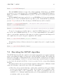
Detailed MCMC example: litters . . . . . . . . . . . . . . . . . . . . .
Higher level usage: MCMC Suite . . . . . . . . . . . . . . . . . . . . .
7.7.1 MCMC Suite example: litters . . . . . . . . . . . . . . . . . . .
7.7.2 MCMC Suite outputs . . . . . . . . . . . . . . . . . . . . . . . .
7.7.3 Custom arguments to MCMC Suite . . . . . . . . . . . . . . . .
Advanced topics . . . . . . . . . . . . . . . . . . . . . . . . . . . . . . .
7.8.1 Custom sampler functions . . . . . . . . . . . . . . . . . . . . .
8 Other algorithms provided by NIMBLE
8.1 Basic Utilities . . . . . . . . . . . . . . . . . . . . . . .
8.1.1 simNodes, calcNodes, and getLogProbs . . . .
8.1.2 simNodesMV, calcNodesMV, and getLogProbsMV
8.2 Particle filter . . . . . . . . . . . . . . . . . . . . . . .
8.3 Monte Carlo Expectation Maximization (MCEM) . . .
.
.
.
.
.
.
.
.
.
.
.
.
.
.
.
.
.
.
.
.
.
.
.
.
.
.
.
.
.
.
.
.
.
.
.
.
.
.
.
.
.
.
.
.
.
.
.
.
.
.
.
.
.
.
.
.
.
.
.
.
.
.
.
.
.
.
.
.
.
.
.
.
.
.
.
.
.
.
.
.
.
.
.
.
.
.
.
.
.
.
60
60
61
61
63
63
64
65
65
69
69
70
71
73
73
.
.
.
.
.
.
.
.
.
.
.
.
.
.
.
76
76
76
78
79
80
.
.
.
.
.
.
.
.
.
.
.
.
.
.
.
.
.
.
.
.
.
82
82
84
84
85
86
87
87
87
88
88
92
92
93
93
94
94
95
96
97
98
100
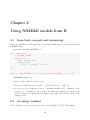
9 Programming with models
9.1 Writing nimbleFunctions . . . . . . . . . . . . . . . . . . . . . . . . . . . .
9.2 Using and compiling nimbleFunctions . . . . . . . . . . . . . . . . . . . . .
9.2.1 Accessing and modifying numeric values from setup . . . . . . . . .
9.3 Compiling numerical operations with no model: omitting setup code . . .
9.4 Useful tools for setup functions . . . . . . . . . . . . . . . . . . . . . . . .
9.4.1 Control of setup outputs . . . . . . . . . . . . . . . . . . . . . . .
9.5 NIMBLE language components . . . . . . . . . . . . . . . . . . . . . . . .
9.5.1 Basics . . . . . . . . . . . . . . . . . . . . . . . . . . . . . . . . . .
9.5.2 Driving models: calculate, simulate, and getLogProb . . . . . . . .
9.5.3 Accessing model and modelValues variables and using copy . . . . .
9.5.4 Using model variables and modelValues in expressions . . . . . . . .
9.5.5 Getting and setting more than one model node or variable at a time
9.5.6 Basic flow control: if-then-else, for, and while . . . . . . . . . . . .
9.5.7 How numeric types work . . . . . . . . . . . . . . . . . . . . . . . .
9.5.8 Declaring argument types and the return type . . . . . . . . . . . .
9.5.9 Querying and changing sizes . . . . . . . . . . . . . . . . . . . . . .
9.5.10 Basic math and linear algebra . . . . . . . . . . . . . . . . . . . . .
9.5.11 Including other methods in a nimbleFunction . . . . . . . . . . . .
9.5.12 Using other nimbleFunctions . . . . . . . . . . . . . . . . . . . . . .
9.5.13 Virtual nimbleFunctions and nimbleFunctionLists . . . . . . . . . .
9.5.14 print . . . . . . . . . . . . . . . . . . . . . . . . . . . . . . . . . . .
CONTENTS
4
9.5.15 Alternative keywords for some functions . . . . . . . . . . . . . . . . 100
9.5.16 User-defined data structures . . . . . . . . . . . . . . . . . . . . . . . 101
9.5.17 distribution functions . . . . . . . . . . . . . . . . . . . . . . . . . . . 102
10 Additional and advanced topics
104
10.1 Cautions and suggestions . . . . . . . . . . . . . . . . . . . . . . . . . . . . . 104
10.2 Parallel processing . . . . . . . . . . . . . . . . . . . . . . . . . . . . . . . . 104
Chapter 1
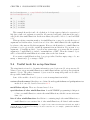
Welcome to NIMBLE
NIMBLE is a system for building and sharing analysis methods for statistical models, especially for hierarchical models and computationally-intensive methods. This is an early
version, 0.3. You can do quite a bit with it, but you can also expect it to be rough and
incomplete. If you want to analyze data, we hope you will find something already useful. If
you want to build algorithms, we hope you will program in NIMBLE and make an R package
providing your method. We also hope you will join the mailing lists (R-nimble.org) and help
improve NIMBLE by telling us what you want to do with it, what you like, and what could
be better. We have a lot of ideas for how to improve it, but we want your help and ideas
too.
1.1
Why something new?
There is a lot of statistical software out there. Why did we build something new? More and
more, statistical models are being customized to the details of each project. That means it
is often difficult to find a package whose set of available models and methods includes what
you need. And more and more, statistical models are hierarchical, meaning they have some
unobserved random variables between the parameters and the data. These may be random
effects, shared frailties, latent states, or other such things. Or a model may be hierarchical
simply due to putting Bayesian priors on parameters. Except for simple cases, hierarchical
statistical models are often analyzed with computationally-intensive algorithms, the best
known of which is Markov chain Monte Carlo (MCMC).
Several existing software systems have become widely used by providing a flexible way to
say what the model is and then automatically providing an algorithm such as MCMC. When
these work, and when MCMC is what you want, that’s great. Unfortunately, there are a lot
of hard models out there for which default MCMCs don’t work very well. And there are also
a lot of useful new and old algorithms that are not MCMC. That’s why we wanted to create
a system that combines a flexible system for model specification – the BUGS language –
with the ability to program with those models. That’s the goal of NIMBLE.
5
CHAPTER 1. WELCOME TO NIMBLE
1.2
6
What does NIMBLE do?
NIMBLE stands for Numerical Inference of statistical Models for Bayesian and Likelihood
Estimation. Although NIMBLE was motivated by algorithms for hierarchical statistical
models, you could use it for simpler models too.
You can think of NIMBLE as comprising three pieces:
1. A system for writing statistical models flexibly, which is an extension of the BUGS
language1 .
2. A library of algorithms such as MCMC.
3. A language, called NIMBLE, embedded within and similar in style to R, for writing
algorithms that operate on BUGS models.
Both BUGS models and NIMBLE algorithms are automatically processed into C++
code, compiled, and loaded back into R with seamless interfaces.
Since NIMBLE can compile R-like functions into C++ that use the Eigen library for fast
linear algebra, it can be useful for making fast numerical functions with or without BUGS
models involved2
One of the beauties of R is that many of the high-level analysis functions are themselves
written in R, so it is easy to see their code and modify them. The same is true for NIMBLE:
the algorithms are themselves written in the NIMBLE language.
1.3
How to use this manual
We emphasize that you can use NIMBLE for data analysis with the algorithms provided
by NIMBLE without ever using the NIMBLE language to write algorithms. So as you get
started, feel free to focus on Chapters 2-8. The algorithm library in v0.3 is just a start, so
we hope you’ll let us know what you want to see and consider writing it in NIMBLE. More
about NIMBLE programming comes in 9.
1
But see Section 5.1.2 for information about limitations and extensions to how NIMBLE handles BUGS
right now.
2
The packages Rcpp and RcppEigen provide different ways of connecting C++, the Eigen library and R.
In those packages you program directly in C++, while in NIMBLE you program in an R-like fashion and
the NIMBLE compiler turns it into C++. Programming directly in C++ allows full access to C++, while
programming in NIMBLE allows simpler code.
Chapter 2
Lightning introduction
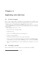
2.1
A brief example
Here we’ll give a simple example of building a model and running some algorithms on the
model, as well as creating our own user-specified algorithm. The goal is to give you a sense
for what one can do in the system. Later sections will provide more detail.
We’ll use the pump model example from BUGS1 . As you’ll see later, we can read the
model into NIMBLE from the files provided as the BUGS example but for now, we’ll enter
it directly in R.
In this “lightning introduction” we will:
1. Create the model for the pump example.
2. Compile the model.
3. Create a basic MCMC specification for the pump model.
4. Compile and run the MCMC
5. Customize the MCMC specification and compile and run that.
6. Create, compile and run a Monte Carlo Expectation Maximization (MCEM) algorithm,
which illustrates some of the flexibility NIMBLE provides to combine R and NIMBLE.
7. Write a short nimbleFunction to generate simulations from designated nodes of any
model.
2.2
Creating a model
First we define the model code, its constants, data, and initial values for MCMC.
1
The data set describes failure times of some pumps.
7
CHAPTER 2. LIGHTNING INTRODUCTION
pumpCode <- nimbleCode({
for (i in 1:N){
theta[i] ~ dgamma(alpha,beta);
lambda[i] <- theta[i]*t[i];
x[i] ~ dpois(lambda[i])
}
alpha ~ dexp(1.0);
beta ~ dgamma(0.1,1.0);
})
pumpConsts <- list(N = 10,
t = c(94.3, 15.7, 62.9, 126, 5.24,
31.4, 1.05, 1.05, 2.1, 10.5))
pumpData <- list(x = c(5, 1, 5, 14, 3, 19, 1, 1, 4, 22))
pumpInits <- list(alpha = 1, beta = 1,
theta = rep(0.1, pumpConsts$N))
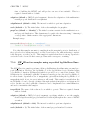
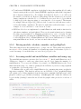
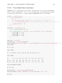
Now let’s create the model and look at some of its nodes.
pump <- nimbleModel(code = pumpCode, name = 'pump', constants = pumpConsts,
data = pumpData, inits = pumpInits)
pump$getNodeNames()
##
##
##
##
##
##
##
##
##
##
##
##
##
##
##
##
##
[1]
[3]
[5]
[7]
[9]
[11]
[13]
[15]
[17]
[19]
[21]
[23]
[25]
[27]
[29]
[31]
[33]
pump$x
"alpha"
"lifted_d1_over_beta"
"theta[2]"
"theta[4]"
"theta[6]"
"theta[8]"
"theta[10]"
"lambda[2]"
"lambda[4]"
"lambda[6]"
"lambda[8]"
"lambda[10]"
"x[2]"
"x[4]"
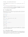
"x[6]"
"x[8]"
"x[10]"
"beta"
"theta[1]"
"theta[3]"
"theta[5]"
"theta[7]"
"theta[9]"
"lambda[1]"
"lambda[3]"
"lambda[5]"
"lambda[7]"
"lambda[9]"
"x[1]"
"x[3]"
"x[5]"
"x[7]"
"x[9]"
8
CHAPTER 2. LIGHTNING INTRODUCTION
##
[1]
5
1
5 14
3 19
1
1
9
4 22
pump$alpha
## [1] 1
pump$theta
##
[1] 0.1 0.1 0.1 0.1 0.1 0.1 0.1 0.1 0.1 0.1
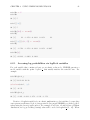
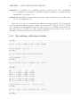
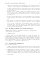
Notice that in the list of nodes, NIMBLE has introduced a new node, lifted d1 over beta.
We call this a “lifted” node. Like R, NIMBLE allows alternative parameterizations, such as
the scale or rate parameterization of the gamma distribution. Choice of parameterization
can generate a lifted node. It’s helpful to know why they exist, but you shouldn’t need to
worry about them.
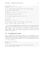
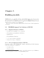
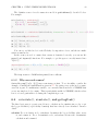
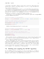
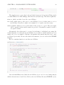
Thanks to the plotting capabilities of the igraph package that NIMBLE uses to represent
the directed acyclic graph, we can plot the model (figure 2.1).
plot(pump$graph)
To simulate from the prior for theta (overwriting the initial values previously in the
model) we first need to fully initialize the model, including any non-stochastic nodes such
as lifted nodes. We do so using NIMBLE’s calculate function and then simulate from the
distribution for theta. First we show how to use the model’s getDependencies method to
query information about its graph.
pump$getDependencies(c('alpha', 'beta'))
## [1] "alpha"
## [3] "lifted_d1_over_beta"
## [5] "theta[2]"
## [7] "theta[4]"
## [9] "theta[6]"
## [11] "theta[8]"
## [13] "theta[10]"
"beta"
"theta[1]"
"theta[3]"
"theta[5]"
"theta[7]"
"theta[9]"
pump$getDependencies(c('alpha', 'beta'), determOnly = TRUE)
## [1] "lifted_d1_over_beta"
set.seed(0) ## This makes the simulations here reproducible
calculate(pump, pump$getDependencies(c('alpha', 'beta'), determOnly = TRUE))
## [1] 0
CHAPTER 2. LIGHTNING INTRODUCTION
10
x[10]
x[1]
x[7]
lambda[10]
lambda[1]
lambda[7]
x[6]
lambda[6]
x[5]
lambda[5]
theta[10]
theta[1]
theta[7]
lambda[4]
theta[6]
theta[4]
beta
alpha
lifted_d1_over_beta
theta[5]
theta[3]
theta[9]
theta[2]
lambda[3]
theta[8]
x[4]
x[3]
lambda[9]
lambda[2]
lambda[8]
x[9]
x[2]
x[8]
Figure 2.1: Directed Acyclic Graph plot of the pump model, thanks to the igraph package
CHAPTER 2. LIGHTNING INTRODUCTION
11
simulate(pump, 'theta')
pump$theta
## the new theta values
##
##
[1] 1.79181 0.29593 0.08369 0.83618 1.22254 1.15836 0.99002
[8] 0.30737 0.09462 0.15720
pump$lambda
##
## lambda hasn't been calculated yet
[1] NA NA NA NA NA NA NA NA NA NA
calculate(pump, pump$getDependencies(c('theta')))
## [1] -286.7
pump$lambda
##
##
## now it has
[1] 168.9674
[7]
1.0395
4.6460
0.3227
5.2641 105.3584
0.1987
1.6506
6.4061
36.3724
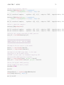
Notice that the first getDependencies call returned dependencies from alpha and beta
down to the next stochastic nodes in the model. The second call requested only deterministic dependencies. We used this as the second argument to calculate. The call to
calculate(pump, ‘theta) expands ‘theta’ to include all nodes in theta. After simulating into ‘theta’, we make sure to calculate its dependencies so they are kept up to date
with the new theta values.
2.3
Compiling the model
Next we compile the model, which means generating C++ code, compiling that code, and
loading it back into R with an object that can be used just like the uncompiled model. The
values in the compiled model will be initialized from those of the original model in R, but
the original and compiled models are distinct objects so any subsequent changes in one will
not be reflected in the other.
Cpump <- compileNimble(pump)
Cpump$theta
##
##
[1] 1.79181 0.29593 0.08369 0.83618 1.22254 1.15836 0.99002
[8] 0.30737 0.09462 0.15720
CHAPTER 2. LIGHTNING INTRODUCTION
2.4
12
Creating, compiling and running a basic MCMC
specification
At this point we have initial values for all of the nodes in the model and we have both the
original and compiled versions of the model. As a first algorithm to try on our model, let’s
use NIMBLE’s default MCMC. Note that all conjugacy is detected for all nodes except for
alpha2 , on which the default sampler is a random walk Metropolis sampler.
pumpSpec <- configureMCMC(pump, print = TRUE)
##
##
##
##
##
##
##
##
##
##
##
##
[1] RW sampler;
targetNode: alpha, adaptive: TRUE, adaptInterval: 200, scale: 1
[2] conjugate_dgamma sampler;
targetNode: beta, dependents_dgamma: theta[1], theta
[3] conjugate_dgamma sampler;
targetNode: theta[1], dependents_dpois: x[1]
[4] conjugate_dgamma sampler;
targetNode: theta[2], dependents_dpois: x[2]
[5] conjugate_dgamma sampler;
targetNode: theta[3], dependents_dpois: x[3]
[6] conjugate_dgamma sampler;
targetNode: theta[4], dependents_dpois: x[4]
[7] conjugate_dgamma sampler;
targetNode: theta[5], dependents_dpois: x[5]
[8] conjugate_dgamma sampler;
targetNode: theta[6], dependents_dpois: x[6]
[9] conjugate_dgamma sampler;
targetNode: theta[7], dependents_dpois: x[7]
[10] conjugate_dgamma sampler;
targetNode: theta[8], dependents_dpois: x[8]
[11] conjugate_dgamma sampler;
targetNode: theta[9], dependents_dpois: x[9]
[12] conjugate_dgamma sampler;
targetNode: theta[10], dependents_dpois: x[10]
pumpSpec$addMonitors(c('alpha', 'beta', 'theta'))
## thin = 1: alpha, beta, theta
pumpMCMC <- buildMCMC(pumpSpec)
CpumpMCMC <- compileNimble(pumpMCMC, project = pump)
niter <- 1000
set.seed(0)
CpumpMCMC$run(niter)
## NULL
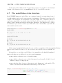
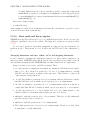
samples <- as.matrix(CpumpMCMC$mvSamples)
par(mfrow = c(1, 4), mai = c(.5, .5, .1, .2))
plot(samples[ , 'alpha'], type = 'l', xlab = 'iteration',
ylab = expression(alpha))
plot(samples[ , 'beta'], type = 'l', xlab = 'iteration',
ylab = expression(beta))
2
This is because we haven’t yet set up NIMBLE to detect conjugate relationships involving an exponential
distribution, but we’ll add that one soon.
CHAPTER 2. LIGHTNING INTRODUCTION
13
0
400
800
0.5
0.0
0
iteration
400
800
0.5
1.0
0.10
0.15
●
●
●
● ●
●
●
● ●
●
●
●●
● ● ●●
●●
●
●
●
●●
●
●
●
●
●
● ●●
●●●
● ● ●
●● ●
●● ●●
● ●●●
●
●
● ●
●●
● ●
●● ●
●
●●
● ●
●●
●
●●●●
●
●
●
● ●●●
●
●●
●
● ●
●●
● ●● ●
●●
●●
●●
●●●
●
●
●
●
●
●
●
●
●
●
● ●● ●
● ●
●●●●
●
● ●●●●●●● ●
●●●
●●
●
●
● ●●●
●
●
●●●●
●
●
●
●
●
●
●
●
●
●
●
●
●●●●
●●●●●●● ● ●
●
●●
●
●●
●
●
●●●
●
●
●●
●
●●
●
●
●
●●
●●
●●●●
●
●●
●
●
●●
●●
●
●
●
●
●
●●
●●
●
●●
●●
●
●
●
●
●
●
●
●
●
●
●
●
●
●
●●
●●●●●●
●
●●● ●
●
●
●
●
●
●
●●
●
●
●
●
●
●
●
●
●
●
●
●
●
●
●
●
●
●
●
●
●
●
●
●
●
●
●● ● ●
●●●
●
●
●●
●●
●
●●●
●
●
●
●
●●
●
●
●
●
●●
●
●
●
●
●
●
●
●
●
●
●●
●
●
●
●●
●
●
●
●
●
●●
●
●
●●
●
●
●
●
●●
●
●
●
●●
●
●
●
●
●
●
●
●
●
●
●
●
●
●
●
●
●
●
●
●
●●●
●●
●
●
●
●
●
●
●
●
●
●
●
●
●
●
●
●
●
●
●
●
●
●●
●
●●●
● ●● ●
●
●
●
●●
●
●
●
●
●
●
●
●
●
●
●
●
●
●
●
●
●
●
●
●
●
●
●
●
●
●
●
●
●●
●●
●
●
●
●●
●
●
●
●
●
●
●
●●
●
●●
●
●
●
●
●
●
●
●
●
●●●
●
●
●
●
●●
●
●
●
●
●
●
●
●
●
●
●
●●
●
●
●
●
●
●
●
●
●
●
●
●
●
●●
●
●
●
●
●
●
●
●
●
●
●
●
●●
●
●
●
●
●
●
●
●
●
●
●
●●
●
●
●
●
●
●●
●
●
●
●
●
●
●
●
●
●
●
●
●
●
●
●
●
●
●
●
●
●
●
●
●
●
●
●
●
●
●
●
●
●
●
●
●
●
●
●
●
●●
●
●●
●
●
●
●
●
●●
●
●
●
●
●
●
●
●
●
●
●
●●●
●●
●
●
●
●
●●
●
●
●
●
●
●
●
●
●
●
●
●●
●
●
●
●
●
●
●●
●●
●
●
●
●
●
●
●
●●
●
●
●
●
●
●
●
●● ● ●
●
●
●
●●●
●
●
●
●
●
●
●
●
●
●●●
●●
●
●
●
●
●● ●
●
0.05
●
θ1
●
3.0
2.5
2.0
1.0
1.5
β
1.5
0.0
0.5
0.5
1.0
β
1.0
α
2.0
2.5
1.5
3.0
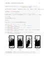
plot(samples[ , 'alpha'], samples[ , 'beta'], xlab = expression(alpha),
ylab = expression(beta))
plot(samples[ , 'theta[1]'], type = 'l', xlab = 'iteration',
ylab = expression(theta[1]))
1.5
α
iteration
0
400
800
iteration
1.0
0.2
0.4
ACF
0.4
0.0
0.0
0.2
ACF
0.6
0.6
0.8
0.8
1.0
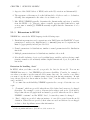
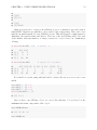
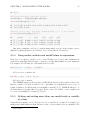
acf(samples[, 'alpha']) ## plot autocorrelation of alpha sample
acf(samples[, 'beta']) ## plot autocorrelation of beta sample
0 5
15
Lag
25
0 5
15
25
Lag
Notice the posterior correlation between alpha and beta. And a measure of the mixing
for each is the autocorrelation for each, shown by the acf plots.
2.5
Customizing the MCMC
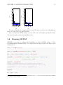
Let’s add an adaptive block sampler on alpha and beta jointly and see if that improves the
mixing.
CHAPTER 2. LIGHTNING INTRODUCTION
14
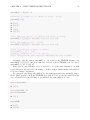
pumpSpec$addSampler('RW_block', list(targetNodes = c('alpha', 'beta'),
adaptInterval = 100))
## [13] RW_block sampler;
targetNodes: alpha, beta,
adaptive: TRUE,
adaptScaleOnly:
pumpMCMC2 <- buildMCMC(pumpSpec)
# need to reset the nimbleFunctions in order to add the new MCMC
CpumpNewMCMC <- compileNimble(pumpMCMC2, project = pump, resetFunctions = TRUE)
set.seed(0);
CpumpNewMCMC$run(niter)
## NULL
samplesNew <- as.matrix(CpumpNewMCMC$mvSamples)
0
400
iteration
800
0
400
iteration
800
●●
●
●
●
●
●● ●●
●
●
●
●
●
●
●●
● ●
● ●
●
●
● ●
●
●
●
●
●
● ●
● ●
● ●● ● ●
●●
●
●●
●●
●●
●●●●
●●
●
● ●●
●
● ●
●●
●
●
●
●
●
●
●
●
●●
●
●●● ● ●
● ●● ●
●●●
●
●●●
●
● ●●
●
●●●●●●
●
●
●●
●
● ●●
●●
●
●
●●
●
●●●
●
●
●
●
●
●●
●
●●
●●
●
●
●
●
●●
●●
●
●
●
●
●●
●●
●
●
●
●●●●
●
●
●
●●●●
●
●●
●
●
●
●
●
●
●
●
●
●
●
●
●
●
●●
● ●●
● ●●●●
●
●●●
●●
●
●
●
●
●
●
●
●
●
●
●
●
●
●
●
●
●
●
●●
●
●
●
●
●
●
●
●
●
●
●
●
●
●
●
●
●
●
●
●
●
●
●
●
●
●
●
●
●
●
●
●
●
● ●●
● ●●
●●●●
●
●●
●
●
●
●
● ●
●●
●
●
●
●
●●
●
●●
●
●
●
●
●●
●
●
●
●●●
●●●
●
● ●●●
●
●●
●●
●
●
●
●
●
●
●
●●●
●
●
●
●
●●● ● ●
●
●
●
●
●
●
●
●
●
●
●
●
●
●
●
●
●
●
●
●
●
●
●
●
●
● ● ●
●
●
●
●
●
●
●
●
●●
●
●
●
●
●
●
●
●●
●
●
●
●
●●
●
●
●
●
●
●
●
●
●
●
●
●
●
●
●
●
●
●
●
●
●
●
●
●
●
●
●
●
●
●● ●
●
●
●
●
●●
●
●
●
●
●
●
●
●
●
●
●
●
●
●
●
●
●
●
●
●●
●
●
●●
●
●
●
●
●
●
●
●
●
●
●
●
●
●
●
●● ●
●
●
●
●
●
●
●
●
●●
●
●
●
●
●
●
●
●
●
●
●
●
●
●
●
●
●
●
●
●
●●
●
●
●
●●●
●
●●
●
●
●
●
●
●
●
●
●
●
●●
●
●
●
●
●
●
●
●
●
●
●
●
●
●●
●
●
●
●●
●
●
●
●
●
●
●
●
●●
●
●
●
●
●
●
●
●
●
●
●
●
●
●
●●
●
●
●
●
●
●
●
●
●
●●
●
●
●
●
●
●
●●
●
●
●● ●
●
●
●
●
●
●
●
●
●
●
●
●
●
●
●
●
●
●
●
●
●
●●
●●
●
●
●
●
●
●
●
●
●
●
●
●
●●
●
●
●
●
●
●
●
●
●
●
●
●
●
●
●
●
●
●
●
●
●●
●
●
●
●
●
●
●
●
●
●
●
●
●
●
●
●
●
●
●
●
●
●
●●
●
●●
●
●●●
●
●
●
●
●
●
●
●
●
●
●
●●
●
●
●
●
●
●
●●
●
●
●
●
● ●
●●
●
●●
●
●
●
●
●
●
●
● ●
●
●
●●●
●
●
●
●
●
●
●
●
●
●
●
●
●
●
●
●
●●
● ●●
●
0.5
1.0
1.5
θ1
0.15
●●
0.10
●
0.05
3.0
2.5
2.0
1.5
0.0
0.5
1.0
β
1.5
0.0
0.5
0.5
1.0
β
1.0
α
2.0
2.5
1.5
3.0
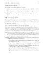
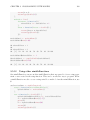
par(mfrow = c(1, 4), mai = c(.5, .5, .1, .2))
plot(samplesNew[ , 'alpha'], type = 'l', xlab = 'iteration',
ylab = expression(alpha))
plot(samplesNew[ , 'beta'], type = 'l', xlab = 'iteration',
ylab = expression(beta))
plot(samplesNew[ , 'alpha'], samplesNew[ , 'beta'], xlab = expression(alpha),
ylab = expression(beta))
plot(samplesNew[ , 'theta[1]'], type = 'l', xlab = 'iteration',
ylab = expression(theta[1]))
0
α
acf(samplesNew[, 'alpha']) ## plot autocorrelation of alpha sample
acf(samplesNew[, 'beta']) ## plot autocorrelation of beta sample
400
iteration
800
1.0
0.0
0.0
0.2
0.4
ACF
0.6
0.6
0.2
0.4
ACF
15
0.8
0.8
1.0
CHAPTER 2. LIGHTNING INTRODUCTION
0 5
15
25
0 5
Lag
15
25
Lag
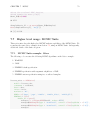
We can see that the block sampler has decreased the autocorrelation for both alpha and
beta. Of course these are just short runs.
Once you learn the MCMC system, you can write your own samplers and include them.
The entire system is written in nimbleFunctions.
2.6
Running MCEM
NIMBLE is a system for working with algorithms, not just an MCMC engine. So let’s
try maximizing the marginal likelihood for alpha and beta using Monte Carlo Expectation
Maximization3 .
pump2 <- pump$newModel()
nodes <- pump2$getNodeNames(stochOnly = TRUE)
box = list( list(c('alpha','beta'), c(0, Inf)))
pumpMCEM <- buildMCEM(model = pump2, latentNodes = 'theta[1:10]',
boxConstraints = box)
pumpMLE <- pumpMCEM()
# Note: buildMCEM returns an R function that contains a
# nimbleFunction rather than a nimble function. That is why
# pumpMCEM() is used instead of pumpMCEM£run().
pumpMLE
##
alpha
3
beta
Note that for this model, one could analytically integrate over theta and then numerically maximize
the resulting marginal likelihood.
CHAPTER 2. LIGHTNING INTRODUCTION
16
## 0.8231 1.2600
Both estimates are within 0.01 of the values reported by George et al. (1993)4
2.7
Creating your own functions
Now let’s see an example of writing our own algorithm and using it on the model. We’ll do
something simple: simulating multiple values for a designated set of nodes and calculating
every part of the model that depends on them.
Here is our nimbleFunction:
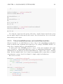
simNodesMany <- nimbleFunction(
setup = function(model, nodes) {
mv <- modelValues(model)
deps <- model$getDependencies(nodes)
allNodes <- model$getNodeNames()
},
run = function(n = integer()) {
resize(mv, n)
for(i in 1:n) {
simulate(model, nodes)
calculate(model, deps)
copy(from = model, nodes = allNodes, to = mv, rowTo = i, logProb = TRUE)
}
})
simNodesTheta1to5 <- simNodesMany(pump, 'theta[1:5]')
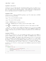
Here are a few things to notice about the nimbleFunction
1. The setup code is written in R. It creates relevant information specific to our model
for use in the run-time code.
2. The run-time is written in NIMBLE. It carries out the calculations using the information determined once for each set of model and nodes arguments by the setup code.
The run-time code is what will be compiled.
3. A modelValues object is created to hold multiple sets of values for variables in the
model provided.
4. The NIMBLE code requires type information about the argument n. In this case it is
a scalar integer.
5. The for-loop looks just like R, but only sequential integer iteration is allowed.
4
George, E.I., Makov, U.E. & Smith, A.F.M. 1993. Conjugate likelihood distributions. Scand. J. Statist.
20:147-156. Their numbers were accidentally swapped in Table 2.
CHAPTER 2. LIGHTNING INTRODUCTION
17
6. The functions calculate and simulate, which were introduced above in R, can be
used in NIMBLE.
7. The special function copy is used here to record values from the model into the modelValues object.
8. One instance, or “specialization”, simNodesTheta1to5, has been made by calling
simNodesMany with the pump model and nodes ‘theta[1:5]’ as arguments. These
are used as inputs to the setup function. What is returned is an object of a uniquely
generated reference class with a run method (member function) that will execute the
run code.
In fact, simNodesMany is very similar to a standard nimbleFunction provided with nimble, simNodesMV.
Now let’s execute this nimbleFunction in R, before compiling it.
set.seed(0) ## make the calculation repeatable
pump$alpha <- pumpMLE[1]
pump$beta <- pumpMLE[2]
calculate(pump, pump$getDependencies(c('alpha','beta'), determOnly = TRUE))
## [1] 0
saveTheta <- pump$theta
simNodesTheta1to5$run(10)
simNodesTheta1to5$mv[['theta']][1:2]
## [[1]]
## [1] 1.43718 1.53094 1.45029 0.03717 0.13310 1.15836 0.99002
## [8] 0.30737 0.09462 0.15720
##
## [[2]]
## [1] 0.34222 3.45823 0.82805 0.08796 0.34440 1.15836 0.99002
## [8] 0.30737 0.09462 0.15720
simNodesTheta1to5$mv[['logProb_x']][1:2]
## [[1]]
## [1] -115.767 -20.856 -73.444
-8.259
-3.570
-7.430
## [7]
-1.001
-1.454
-9.841 -39.097
##
## [[2]]
## [1] -19.688 -50.300 -37.108 -2.598 -1.825 -7.430 -1.001
## [8] -1.454 -9.841 -39.097
In this code we have initialized the values of alpha, beta, to their MLE, and recorded the
theta values to use next. Then we have requested 10 simulations from simNodesTheta1to5.
CHAPTER 2. LIGHTNING INTRODUCTION
18
Shown are the first two simulation results for theta and the log probabilities of x. Notice that
theta[6:10] and the corresponding log probabilities for x[6:10] are unchanged because the
nodes being simulated are only theta[1:5]. In R, this function runs slowly.
Finally, let’s compile the function and run that version.
CsimNodesTheta1to5 <- compileNimble(simNodesTheta1to5,
project = pump, resetFunctions = TRUE)
Cpump$alpha <- pumpMLE[1]
Cpump$beta <- pumpMLE[2]
calculate(Cpump, Cpump$getDependencies(c('alpha','beta'), determOnly = TRUE))
## [1] 0
Cpump$theta <- saveTheta
set.seed(0)
CsimNodesTheta1to5$run(10)
## NULL
CsimNodesTheta1to5$mv[['theta']][1:2]
## [[1]]
## [1] 1.43718 1.53094 1.45029 0.03717 0.13310 1.15836 0.99002
## [8] 0.30737 0.09462 0.15720
##
## [[2]]
## [1] 0.34222 3.45823 0.82805 0.08796 0.34440 1.15836 0.99002
## [8] 0.30737 0.09462 0.15720
CsimNodesTheta1to5$mv[['logProb_x']][1:2]
## [[1]]
## [1] -115.767 -20.856 -73.444
-8.259
-3.570
-2.593
## [7]
-1.006
-1.180
-1.757
-2.532
##
## [[2]]
## [1] -19.688 -50.300 -37.108 -2.598 -1.825 -2.593 -1.006
## [8] -1.180 -1.757 -2.532
Given the same initial values and the same random number generator seed, we got identical results, but it happened much faster.
Chapter 3
More Introduction
Now that we have shown a brief example, we will introduce more about the concepts and
design of NIMBLE. Subsequent chapters will go into more detail about working with models
and programming in NIMBLE.
One of the most important concepts behind NIMBLE is to allow a combination of highlevel processing in R and low-level processing in compiled C++. For example, when we
write a Metropolis-Hastings MCMC sampler in the NIMBLE language, the inspection of
the model structure related to one node is done in R, and the actual sampler calculations
are done in compiled C++. The theme of separating one-time high-level processing and
repeated low-level processing will become clearer as we introduce more about NIMBLE’s
components.
3.1
NIMBLE adopts and extends the BUGS language
for specifying models
We adopted the BUGS language, and we have extended it to make it more flexible. The
BUGS language originally appeared in WinBUGS, then in OpenBUGS and JAGS. These
systems all provide automatically-generated MCMC algorithms, but we have adopted only
the language for describing models, not their systems for generating MCMCs. In fact, if you
want to use those or other MCMCs in combination with NIMBLE’s other algorithms, you
can1 . We adopted BUGS because it has been so successful, with over 30,000 registered users
by the time they stopped counting, and with many papers and books that provide BUGS
code as a way to document their statistical models. To learn the basics of BUGS, we refer
you to the OpenBUGS or JAGS web sites. For the most part, if you have BUGS code, you
can try NIMBLE.
NIMBLE takes BUGS code and does several things with it:
1. NIMBLE extracts all the declarations in the BUGS code to create a model definition.
This includes a directed acyclic graph (DAG) representing the model and functions
that can inspect the graph and model relationships. Usually you’ll ignore the model
definition and let NIMBLE’s default options take you directly to the next step.
1
and will be able to do so more thoroughly in the future
19
CHAPTER 3. MORE INTRODUCTION
20
2. From the model definition, NIMBLE builds a working model in R. This can be used
to manipulate variables and operate the model from R. Operating the model includes
calculating, simulating, or querying the log probability value of model nodes. These
basic capabilities, along with the tools to query model structure, allow one to write
programs that use the model and adapt to its structure.
3. From the working model, NIMBLE generates customized C++ code representing the
model, compiles the C++, loads it back into R, and provides an R object that interfaces
to it. We often call the uncompiled model the “R-model” and the compiled model the
“C-model.” The C-model can be used identically to the R-model, so code written to
use one will work with the other. We use the word “compile” to refer to the entire
process of generating C++ code, compiling it and loading it into R.
You’ll learn more about specifying and manipulating models in Chapter 5-6.
3.2
The NIMBLE language for writing algorithms
NIMBLE provides a language, embedded within and similar in style to R, for writing algorithms that can operate on BUGS models. The algorithms can use NIMBLE’s utilities for
inspecting the structure of a model, such as determining the dependencies between variables.
And the algorithms can control the model, changing values of its variables and controlling
execution of its probability calculations or corresponding simulations. Finally, the algorithms
can use automatically generated data structures to manage sets of model values and probabilities. In fact, the calculations of the model are themselves constructed as functions in the
NIMBLE language, as are the algorithms provided in NIMBLE’s algorithm library. This will
make it possible in the future to extend BUGS with new distributions and new functions
written in NIMBLE.
Like the models themselves, functions in the NIMBLE language are turned into C++,
which is compiled, loaded, and interfaced to R.
Programming in NIMBLE involves a fundamental distinction between:
1. the steps for an algorithm that need to happen only once, at the beginning, such as
inspecting the model; and
2. the steps that need to happen each time a function is called, such as MCMC iterations.
Programming in NIMBLE allows, and indeed requires, these steps to be given separately.
When one writes a nimbleFunction, each of these parts can be provided. The former, if
needed, are given in a setup function, and they are executed directly in R, allowing any
feature of R to be used. The latter are in one or more run-time functions, and they are
turned into C++. Run-time code is written in the NIMBLE language, which you can think
of as a carefully controlled, small subset of R along with some special functions for handling
models and NIMBLE’s data structures.
What NIMBLE does with a nimbleFunction is similar to what it does with a BUGS
model:
CHAPTER 3. MORE INTRODUCTION
21
1. NIMBLE creates a working R version of the nimbleFunction, which you can use with
an R-model or a C-model.
2. NIMBLE generates C++ code for the run-time function(s), compiles it, and loads it
back into R with an interface nearly identical to the R version of the nimbleFunction.
As for models, we refer to the uncompiled and compiled versions as R-nimbleFunctions
and C-nimbleFunctions, respectively. In v0.3, the behavior of nimbleFunctions is
usually very similar, but not identical, between the two versions.
You’ll learn more about writing algorithms in Chapter 9.
3.3
The NIMBLE algorithm library
In v0.3, the NIMBLE algorithm library is fairly limited. It includes:
1. MCMC with samplers including conjugate, slice, adaptive random walk, and adaptive
block. NIMBLE’s MCMC system illustrates the flexibility of combining R and C++.
An R function inspects the model object and creates an MCMC specification object
representing choices of which kind of sampler to use for each node. This MCMC
specification can be modified in R, such as adding new samplers for particular nodes,
before compiling the algorithm. Since each sampler is written in NIMBLE, you can
use its source code or write new samplers to insert into the MCMC. And if you want
to build an entire MCMC system differently, you could do that too.
2. A nimbleFunction that provides a likelihood function for arbitrary sets of nodes in
any model. This can be useful for simple maximum likelihood estimation of nonhierarchical models using R’s optimization functions. And it can be useful for other R
packages that run algorithms on any likelihood function.
3. A nimbleFunction that provides ability to simulate, calculate, or retrieve the summed
log probability (density) of many sets of values for arbitrary sets of nodes.
4. A basic Monte Carlo Expectation Maximization (MCEM) algorithm. MCEM has its
issues as an algorithm, such as potentially slow convergence to maximum likelihood
(i.e. empirical Bayes in this context) estimates, but we chose it as a good illustration of
how NIMBLE can be used. Each MCMC step uses NIMBLE’s MCMC; the objective
function for maximization is another nimbleFunction; and the actual maximization
is done through R’s optim function2 .
You’ll learn more about the NIMBLE algorithm library in Chapter 8.
2
In the future we plan to provide direct access to R’s optimizers from within nimbleFunctions
Chapter 4
Getting started
4.1
Requirements to run NIMBLE
You can run NIMBLE on any of the three common operating systems: Linux, Mac, or
Windows.
The following are required to run NIMBLE.
1. R, of course.
2. The igraph R package.
3. A working C++ compiler that R can use on your system. There are standard opensource C++ compilers that the R community has already made easy to install. You
don’t need to know anything about C++ to use NIMBLE.
NIMBLE also uses a couple of C++ libraries that you don’t need to install, as they will
already be on your system or are provided by NIMBLE.
1. The Eigen C++ library for linear algebra. This comes with NIMBLE, or you can use
your own copy.
2. The BLAS and LAPACK numerical libraries. These come with R.
Most fairly recent versions of these requirements should work.
4.2
Installation
Since NIMBLE is an R package, you can install it in the usual way, via install.packages()
or related mechanisms. We have not yet put in on CRAN, so you’ll have to find it at Rnimble.org.
For most installations, you can ignore low-level details. However, there are some options
that some users may want to utilize.
22
CHAPTER 4. GETTING STARTED
4.2.1
23
Using your own copy of Eigen
NIMBLE uses the Eigen C++ template library for linear algebra (http://eigen.tuxfamily.
org/index.php?title=Main_Page)). Version 3.2.1 of Eigen is included in the NIMBLE
package and that version will be used unless the package’s configuration script finds another
version on the machine. This works well, and the following is only relevant if you want to
use a different (e.g., newer) version.
The configuration script looks in the standard include directories, e.g. /usr/include
and /usr/local/include for the header file Eigen/Dense. You can specify a particular
location in either of two ways:
1. Set the environment variable EIGEN DIR before installing the R package, e.g., export
EIGEN DIR=/usr/include/eigen3 in the bash shell.
2. Use R CMD INSTALL --configure-args='--with-eigen=/path/to/eigen' nimble or
install.packages("nimble", configure.args = "--with-eigen=/path/to/eigen").
In these cases, the directory should be the full path to the directory that contains the Eigen
directory, e.g. /usr/local/include. It is not the full path to the Eigen directory itself, i.e.,
NOT /usr/local/include/Eigen.
4.2.2
Using libnimble
NIMBLE generates specialized C++ code for user-specified models and nimbleFunctions.
This code uses some NIMBLE C++ library classes and functions. By default, on Linux and
OS X, the library code is compiled once as a linkable library - libnimble. This single instance
of the library is then linked with the code for each generated model. Alternatively, one can
have the library code recompiled in each model’s own dynamically loadable library (DLL).
This does repeat the same code across models and so occupies more memory. There may be
a marginal speed advantage. This is currently what happens on Windows. One can disable
using libnimble via the configuration argument --enable-lib, e.g.
R CMD INSTALL --configure-args='--enable-lib=false' nimble
4.2.3
LAPACK and BLAS
NIMBLE also uses BLAS and LAPACK for some of its linear algebra (in particular calculating density values and generating random samples from multivariate distributions).
NIMBLE will use the same BLAS and LAPACK installed on your system that R uses. Note
that a fast (and where appropriate, threaded) BLAS can greatly increase the speed of linear
algebra calculations. See Section A.3.1 of the R Installation and Administration manual for
more details on providing a fast BLAS for your R installation.
4.2.4
Problems with Installation
We have tested the installation on the three commonly used platforms – OS X, Linux,
Windows 7. We don’t anticipate problems with installation, but we want to hear about any
CHAPTER 4. GETTING STARTED
24
and help resolve them. Please post about installation problems to the nimble-users Google
group or email [email protected].
4.2.5
RStudio and NIMBLE
You can use NIMBLE in RStudio, but we strongly recommend that you turn off the option
to display the Global Environment. Leaving it on can cause RStudio to freeze, apparently
from trying to deal with some of NIMBLE’s data structures.
4.3
Installing a C++ compiler for R to use
In addition to needing a C++ compiler to install the package (from source), you also need to
have a C++ compiler and the utility make at run-time. This is needed during the R session
to compile the C++ code that NIMBLE generates for a user’s models and algorithms.
4.3.1
OS X
On OS X, you should install Xcode. The command-line tools, which are available as a
smaller installation, should be sufficient. This is freely available from the Mac App Store. See
https://developer.apple.com/xcode/downloads/ and https://itunes.apple.com/us/
app/xcode/id497799835?ls=1&mt=12
4.3.2
Linux
On Linux, you can install the GNU compiler suite (gcc/g++). You can use the package
manager to install pre-built binaries. On Ubuntu, the following command will install or
update make, gcc and libc.
sudo apt-get install build-essential
4.3.3
Windows
On Windows, you should download and install Rtools.exe available from http://cran.
r-project.org/bin/windows/Rtools/. Select the appropriate executable corresponding
to your version of R. (We strongly recommend using the most recent version of R, currently
3.1.0, and hence Rtools31.exe). This installer leads you through several “pages”. You can
accept all of the defaults. It is essential the checkbox for the “R 2.15+ toolchain” (page 4)
is enabled in order to have gcc/g++, make, etc. installed. Also, we recommend that you
check the PATH checkbox (page 5). This will ensure that R can locate these commands.
CHAPTER 4. GETTING STARTED
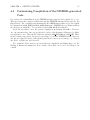
4.4
25
Customizing Compilation of the NIMBLE-generated
Code
For each model or nimbleFunction, the NIMBLE package generates and compiles C++ code.
This uses classes and routines available through the NIMBLE run-time library and also the
Eigen library. The compilation mechanism uses R’s SHLIB functionality and so the regular
R configuration in ${R_HOME}/etc${R_ARCH}/Makeconf. NIMBLE places a Makevars file in
the directory in which the code is generated and R CMD SHLIB uses this file.
In all but specialized cases, the general compilation mechanism will suffice. However,
one can customize this. One can specify the location of an alternative Makevars (or Makevars.win) file to use. That should define the variables PKG CPPFLAGS and PKG LIBS. These
should contain, respectively, the pre-processor flag to locate the NIMBLE include directory,
and the necessary libraries to link against (and their location as necessary), e.g., Rlapack
and Rblas on Windows, and libnimble.
Use of this file allows users to specify additional compilation and linking flags. See the
Writing R Extensions manual for more details of how this can be used and what it can
contain.
Chapter 5
Building models
NIMBLE aims to be compatible with the original BUGS language and also the version
used by the popular JAGS package, as well as to extend the BUGS language. However, at
this point, there are some BUGS features not supported by NIMBLE, and there are some
extensions that are planned but not implemented.
Here is an overview of the status of BUGS features, followed by more detailed explanations
of each topic.
5.1
5.1.1
NIMBLE support for features of BUGS
Supported features of BUGS
1. Stochastic and deterministic1 node declarations.
2. Most univariate and multivariate distributions
3. Link functions
4. Most mathematical functions
5. “for” loops for iterative declarations.
6. Arrays of nodes up to 3 dimensions.
5.1.2
Not-yet-supported features of BUGS
Eventually, we plan to make NIMBLE fully compatible with BUGS and JAGS. In this first
release, the following are not supported.
1. Stochastic indices
2. The I() notation
1
NIMBLE calls non-stochastic nodes “deterministic”, whereas BUGS calls them “logical”. NIMBLE uses
“logical” in the way R does, to refer to boolean (TRUE/FALSE) variables.
26
CHAPTER 5. BUILDING MODELS
27
3. Aspects of the JAGS dialect of BUGS, such as the T() notation and dinterval().
4. The appearance of the same node on the left-hand side of both a <- and a ∼ declaration,
allowing data assignment for the value of a stochastic node.
5. Like BUGS, NIMBLE generally determines the dimensionality and sizes of variables
from the BUGS code. However, when a variable appears with blank indices, such
as in x.sum <- sum(x[]), NIMBLE currently requires that the dimensions of x be
provided.
5.1.3
Extensions to BUGS
NIMBLE also extends the BUGS language in the following ways:
1. Distribution parameters can be expressions, as in JAGS but not in WinBUGS2 . Caveat:
parameters to multivariate distributions (e.g., dmnorm()) may not be expressions, but
must be [appropriately indexed] model nodes.
2. Named parameters for distributions, similar to named parameters in R’s distribution
functions.
3. Multiple parameterizations for distributions, similar to those in R.
4. More flexible indexing of vector nodes within larger variables, such as placing a multivariate normal vector arbitrarily within a higher-dimensional object, not just in the
last index.
Extension for handling “data”
In BUGS, when you define a model, you provide the data for the model. You can use
NIMBLE that way too, but NIMBLE provides more flexibility. Consider, for example, a
case where you want to use the same model for many data sets. Or, consider a case where
you want to use the model to simulate many data sets from known parameters. In such
cases, the model needs to know what nodes have “data”3 , but the values of the data nodes
can be modified.
To accommodate such flexibility, NIMBLE separates the concept of data into two concepts:
1. “Constants”, which are provided when the model is defined and can never be changed
thereafter. For example, a vector of known index values, such as for block indices,
helps define the model graph itself and must be provided when the model is defined.
NIMBLE “constants” are like BUGS “data”, because they cannot be changed.
2. “Data”, which are provided when an instance of a model is created from the model
definition. When data are provided, their values are used and their nodes are flagged
as data so that algorithms can use that information.
2
3
e.g., y
dnorm(5 + mu, 3 * exp(tau))
because algorithms will want to query the model about its nodes
CHAPTER 5. BUILDING MODELS
28
Future extensions to BUGS
We also plan to extend the BUGS language to support:
1. Ability to provide new functions and new distributions written NIMBLE.
2. If-then-else syntax for one-time evaluation when the model is compiled, so that the
same model code can generate different models when different conditions are met.
3. Single-line declaration of common motifs such as GLMs, GLMMs, and time-series
models.
5.2
Creating models
Here we describe in detail two ways to provide a BUGS model for use by NIMBLE. The first,
nimbleModel, is the primary way to do it and was illustrated in Chapter 2 . The second,
readBUGSmodel provides compatibility with BUGS file formats for models, variables, data,
and initial values for MCMC.
5.2.1
Using nimbleModel() to specify a model
There are five arguments to nimbleModel that provide information about the model, of
which code is the only required one. Understanding these arguments involves some basic
concepts about NIMBLE and ways it differs from BUGS and JAGS, so we explain them
here. The R help page (?nimbleModel) provides a reference for this information.
code This is R code for the BUGS model. With just a few exceptions such as T() and
I() notation, BUGS code is syntactically compatible with R, so it can be held in an
R object. There are three ways to make such an object, by using nimbleCode(), the
synonym BUGScode(), or simply the R function quote().
constants This is a named list of values that cannot be modified after creating the model
definition. They may include constants such as
1. N in the pump example, which is required for processing the BUGS code since it
appears in for(i in 1:N).
2. vectors of indices, such as when the model has nodes like y[i] ∼ dnorm(mu[blockID[i]
], sd), where blockID is a vector of experimental block IDs that indicate which
mu is needed for each y. Since vectors of indices are used to define the model
graph, they cannot be changed after model definition
3. actual data, if they will never be changed. Note that data may alternatively be
provided via the data argument or the setData member function, in which case
the model knows those nodes represent data, but their values may be changed.
This allows the same model to be used to analyze or to simulate multiple data
sets.
CHAPTER 5. BUILDING MODELS
29
dimensions This is a named list of vectors of the sizes of variables that appear in the
model with unfilled indices such as x[,]. For the most part, NIMBLE determines the
sizes of model variables automatically, but in cases with blank index fields, dimension
information is required. As described in the section below about indexing, NIMBLE
currently requires square brackets with blank indices (or complete indicies such as
1:N, of course) when the full extent of a variable is needed. The dimension argument
for x[,] would be e.g. list(x = c(10, 8)) if x is a 10-by-8 matrix. Dimension
information can alternatively be taken from constants or data if these are provided.
4
data This is a named list of values to be used as data, with NAs to indicate missing data.
inits This is a named list of initial values for the model. These are neither data nor constants, but rather values with which to initialize the model.
5.2.2
More about specifying data nodes and values
NIMBLE distinguishes between constants and data
As described in section 5.1.3, NIMBLE considers constants to be values that will never
change and data to be information about the role a node plays in the model. Nodes marked
as data will by default be protected from any functions that would simulate over their values,
but it is possible to do so or to change their values by direct assignment. Attempting to
change the values of constants after building a model can lead to errors.
Providing data via setData
Whereas the constants are a property of the model definition – since they may help determine
the model structure itself – data nodes can be different in different copies of the model
generated from the same model definition. For this reason, data is not required to be provided
when the model code is processed. It can be provided later via the model member function
setData. e.g., pump$setData(pumpData), where pumpData is a named list of data values.
setData does two things: it sets the values of the data nodes, and it flags those nodes
as containing data so that NIMBLE’s simulate() functions do not overwrite data values.
Values of data variables can be replaced normally, and the indication of which nodes should
be treated as data can be reset by using the resetData method, e.g. pump$resetData().
Since values passed into the constants argument of nimbleModel() can never be modified, they are also marked as data in a model so that algorithms will be prevented from
trying to simulate into them.
4
We have also seen cases where the dimension information inferred from the BUGS code does not match
the data matrix because the model only applies to a subset of the data matrix. In a case like that, either
dimensions must be provided to fit the entire data matrix or only the appropriate subset of the data matrix
must be used in the model.
CHAPTER 5. BUILDING MODELS
30
Missing data values
When a variable that functions as data in a model has missing values, one should set the
nodes whose values are missing to be NA, either through the data argument when creating
a model or via setData. The result will be that nodes with non-NA values will be flagged as
data nodes, while nodes with NA values will not. Note that a node following a multivariate
distribution must be either entirely observed or entirely missing.
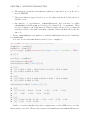
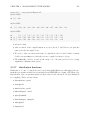
Here’s an example of running an MCMC on the pump model, with two of the observations
taken to be missing. Our default MCMC specification will treat the missing values as
unknowns to be sampled, as can be seen in the MCMC output here.
pumpMiss <- pump$newModel()
pumpMiss$resetData()
pumpDataNew <- pumpData
pumpDataNew$x[c(1, 3)] <- NA
pumpMiss$setData(pumpDataNew)
pumpMissSpec <- configureMCMC(pumpMiss)
pumpMissSpec$addMonitors(c('x', 'alpha', 'beta', 'theta'))
## thin = 1: alpha, beta, x, theta
pumpMissMCMC <- buildMCMC(pumpMissSpec)
Cobj <- compileNimble(pumpMiss, pumpMissMCMC)
niter <- 1000
set.seed(0)
Cobj$pumpMissMCMC$run(niter)
## NULL
samples <- as.matrix(Cobj$pumpMissMCMC$mvSamples)
samples[1:5, 13:17]
##
##
##
##
##
##
[1,]
[2,]
[3,]
[4,]
[5,]
x[1] x[2] x[3] x[4] x[5]
17
1
2
14
3
11
1
4
14
3
14
1
9
14
3
11
1
24
14
3
9
1
29
14
3
CHAPTER 5. BUILDING MODELS
5.2.3
31
Using readBUGSmodel() to specify a model
readBUGSmodel() can read in the model, data/constant values and initial values in formats
mostly compatible with the bugs() and jags() functions in the R2WinBUGS and R2jags
packages. It can also take information directly from R objects, somewhat more flexibly than
nimbleModel(). After processing the file inputs, it calls nimbleModel().
readBUGSmodel() can take the following arguments:
model is either a file name, an R code object such as can be passed in the code argument
of nimbleModel(), or a R function whose body contains the model code.
data is either a file name or a named list specifying constants and data together, the way
they would be provided for BUGS or JAGS. readBUGSmodel() treats values that appear on the left-hand side of BUGS declarations as data and other values as constants,
so you do not need to call the setData method.
inits is either a file name or a named list of initial values.
For both data and inits, if a file is specified, the file should contain R code that creates
objects analogous to what would populate the list if a list were provided instead. Please
see the JAGS manual examples or the classic bugs directory in the NIMBLE package for
example syntax. NIMBLE does not handle formatting such as in some of the original BUGS
examples in which data was indicated with syntax such as data x in ‘x.txt’. Only a
single set of initial values can specified in creating a model; multiple sets of initial values will
(eventually) be handled in NIMBLE’s MCMC implementation.
Example using readBUGSmodel
Let’s create a model for the pump example from BUGS.
pumpDir <- system.file('classic-bugs', 'vol1', 'pump', package = 'nimble')
pumpModel <- readBUGSmodel('pump.bug', data = 'pump-data.R',
inits = 'pump-init.R', dir = pumpDir)
Note that readBUGSmodel() allows one to include var and data blocks in the model file
as in some of the BUGS examples (such as inhaler). The data block pre-computes constant
and data values. NIMBLE by and large does not need the information given in a var block
but occasionally this is used to determine dimensionality, such as in the case of syntax like
xbar <- mean(x[]) where x is a variable that appears only on the right-hand side of BUGS
expressions.
5.2.4
A note on introduced nodes
In some cases, NIMBLE introduces new nodes into the model that were not specified in
the BUGS code for the model, such as the lifted d1 over beta node in the introductory
example. For this reason, it is important that programs written to adapt to different model
CHAPTER 5. BUILDING MODELS
32
structures use NIMBLE’s systems for querying the model graph. For example, a call to
pump$getDependencies("beta") will correctly include lifted d1 over beta in the results.
If one skips this step and assumes the nodes are only those that appear in the BUGS code,
one may not get correct results.
It can be helpful to know the situations in which lifted nodes are generated. These
include:
• When distribution parameters are expressions, NIMBLE creates a new deterministic
node that contains the expression for a given parameter. The node is then a direct
descendant of the new deterministic node. This is an optional feature, but it is currently
enabled in all cases.
• As discussed in 5.3.4 the use of link functions causes new nodes to be introduced.
• Use of alternative parameterizations of distributions. For example when a user provides the precision of a normal distribution as tau, NIMBLE creates a new node sd <1/sqrt(tau) and uses sd as a parameter in the normal distribution. If many nodes use
the same tau, only one new sd node will be created, so the computation 1/sqrt(tau)
will not be repeated redundantly. More about NIMBLE’s parameterizations is described below.
5.3
5.3.1
More details on NIMBLE support of BUGS features
Distributions
NIMBLE supports most of the distributions allowed in BUGS and JAGS. Table 5.1 lists the
distributions currently supported.
To understand how NIMBLE handles alternative parameterizations, it is useful to distinguish three cases, using the gamma distribution as an example:
1. A canonical parameterization is used directly for computations. Usually this is the
parameterization in the Rmath header of R’s C implementation of distributions. For
gamma, this is (shape, scale).
2. The BUGS parameterization is the one defined in the original BUGS language. For
gamma, this is (shape, rate).
3. An alternative parameterization is one that must be converted into the canonical parameterization. For example, NIMBLE provides a (mean, sd) parameterization and
creates nodes to calculate (shape, scale) from (mean, sd). In the case of gamma, the
BUGS parameterization is also an alternative parameterization.
Since NIMBLE aims to provide compatibility with existing BUGS and JAGS code, the
order of parameters places the BUGS parameterization first. For example, the NIMBLE
definition of a gamma, in R format, is dgamma( shape, rate, scale, mean, sd). Like R,
CHAPTER 5. BUILDING MODELS
33
if parameter names are not given, they are taken in order, so that (shape, rate) is the default.
This happens to match R’s order of parameters, but it need not. If names are given, they
can be given in any order. NIMBLE knows that rate is an alternative to scale and that
(mean, sd) are an alternative to (shape, scale or rate).
The file distsDefs table.R in the R directory of the source package is the definitive source
for the NIMBLE’s distributions and parameterizations.
We plan to, but do not currently, handle the following distributions: double exponential
(Laplace), beta-binomial, Dirichlet-multinomial, F, Pareto, inverse Wishart, and various
forms of multivariate t.
We will shortly add the distribution aliases allowed in JAGS: dbinom, dnbinom, dweibull,
ddirich.
CHAPTER 5. BUILDING MODELS
Name
Bernoulli
Beta
Binomial
Categorical
Chi-square
Dirichlet
Exponential
Gamma
Logistic
Log-normal
Multinomial
Multivariate
normal
Negative
binomial
Normal
Poisson
Student t
Uniform
Weibull
Wishart
34
Usage
dbern(prob = p)
0<p<1
dbeta(shape1 = a, shape2 = b)
a > 0, b > 0
dbin(prob = p, size = n)
0 < p < 1, n ∈ N∗
dcat(prob = p)
p ∈ (R+ )N
dchisq(df = k)
k>0
ddirch(alpha)
αj ≥ 0
dexp(rate = lambda)
λ>0
dgamma(shape = r, rate = λ)
λ > 0, r > 0
dlogis(location = µ, rate = τ )
τ >0
dlnorm(mu, tau)
τ >0
dmulti(prob = b,size = n)
P
j xj = n
dmnorm(mu, prec = Λ)
Λ positive definite
dnegbin(prob = p, size = r)
0 < p ≤ 1, r ≥ 0
dnorm(mu, tau)
τ >0
dpois(lambda)
λ>0
dt(mu, tau, df = k)
τ > 0, k > 0
dunif(min = a,max = b)
a<b
dweib(shape = v, lambda)
v > 0, λ > 0
dwish(R, df = k)
R p × p pos. def., k ≥ p
Density
Lower
0
Upper
1
xa−1 (1 − x)b−1
β(a, b)
n x
n−x
x p (1 − p)
0
1
0
n
Ppx
i pi
1
N
x 2 −1 exp(−x/2)
k
2 2 Γ( k2 ) α −1
P
Q x j
Γ( i αi ) j j
Γ(αj )
0
px (1 − p)1−x
k
λ exp(−λx)
λr xr−1 exp(−λx)
Γ(r)
τ exp{(x − µ)τ }
[1 + exp{(x − µ)τ }]2
1
τ 2 −1
x exp −τ (log(x) − µ)2 /2
2π
0
0
0
0
x
Q p j
n! j j
xj !
d
1
(2π)− 2 |Λ| 2 exp{−(x − µ)T Λ(x − µ)/2}
x+r−1
x
τ
2π
Γ( k+1
)
2
Γ( k2 )
1
2
pr (1 − p)x
0
exp{−τ (x − µ)2 /2}
exp(−λ)λx
x!
o− (k+1)
1 n
2
τ (x−µ)2
τ 2
1
+
kπ
k
0
1
b−a
a
vλxv−1 exp(−λxv )
0
|x|(k−p−1)/2 |R|k/2 exp{−tr(Rx/2)}
2pk/2 Γp (k/2)
Table 5.1: Distributions with their default order of parameters. The value of the random
variable is denoted by x.
b
CHAPTER 5. BUILDING MODELS
5.3.2
35
List of parameterizations
NIMBLE extends BUGS by allowing different standard parameterizations of distributions.
These are listed in Table 5.2.
Alternative Parameterization
dbeta(mean, sd)
dexp(scale)
dgamma(shape, scale)
dgamma(mean, sd)
dweib(shape, scale)
dweib(shape, rate)
dlnorm(mu, sd)
dlogis(location, scale)
dnorm(mu, sd)
dnorm(mu, var)
dt(mu, sigma, df)
dmnorm(mu, cov)
dmnorm(mu, chol)
dwish(S, df)
NIMBLE re-parameterization
dbeta(shape1 = mean^2 * (1 - mean) / sd^2 - mean,
shape2 = mean * (1 - mean)^2 / sd^2 + mean - 1)
dexp(rate = 1/scale)
none
dgamma(shape = mean^2 / sd^2, scale = sd^2 / mean)
none
dweib(shape, scale = 1/rate)
none
none
none
dnorm(mu, sd = sqrt(var))
none
dnorm(mu, chol = chol(cov), prec param = FALSE)
dnorm(mu, chol, prec param = FALSE)
dwish(chol = chol(S), df, scale param = TRUE)
Table 5.2: Alternative distribution parameterizations. The first column indicates the supported parameterizations for distributions given in Table 5.1 with their BUGS parameterization. The second column indicates the relationship to the canonical parameterization used
in NIMBLE. In cases where the the BUGS parameterization is not the canonical one, the
latter is listed in this table with none in the second column.
5.3.3
List of BUGS language functions
NIMBLE provides a wide variety of operators and functions for use in defining models (Tables
5.3-5.4). Note that by virtue of how we set up models using the NIMBLE language, these
are the same operators and functions that one can use in a NIMBLE function, as discussed
further in Chapter 9.
For the most part NIMBLE supports the functions used in BUGS and JAGS, with exceptions indicated in the table. Additional functions provided by NIMBLE are also listed. For
distribution functions, currently “r” and “d” functions are provided for each distribution,
and when called from nimbleFunctions only the BUGS parameterization is available in
v0.3, and in fact sometimes that is provided differently. See 9.5.17. Currently “r” functions
only return one random draw at a time, and the first argument must always be 1. For multivariate distribution functions the prec param or scale param argument must be provided,
indicating when a covariance or precision matrix has been given. In a future release we will
provide a variety of distribution functions, including density, cumulative distribution and
CHAPTER 5. BUILDING MODELS
36
quantile functions, using the same syntax as dnorm, pnorm, qnorm. We will also extend the
alternative parameterizations with named parameters to nimbleFunctions.
5.3.4
List of link functions
NIMBLE allows the link functions listed in Table 5.5.
Link functions are specified as functions applied to a variable on the left hand side of
a BUGS expression. To handle link functions, NIMBLE does some processing that inserts an additional node into the model. For example, the declaration logit(p[i]) ∼
dnorm(mu[i],1), is equivalent to the follow two declarations:
• logit p[i] ∼ dnorm(mu[i], 1),
• p[i] <- expit(logit p[i])
where expit is the inverse of logit. When the BUGS expression defines a deterministic
node, such as logit(p) <- b0 + b1*x, the same operations are performed except that
logit p is a deterministic node.
5.3.5
Indexing
NIMBLE allows flexible indexing that is compatible with BUGS and JAGS.
In particular NIMBLE allows
• x[i]
• x[i:j]
• x[i:j,k:l] and indexing of higher dimensional arrays
• x[i:j, ]
• x[3*i+7]
• x[(3*i):(5*i+1)]
When calling functions such as mean and sum on a vector variable, the square brackets
are required but can have blank indices, e.g. xbar <- mean(x[]) if x is a vector and xbar
<- mean(x[,]) if x is a matrix 5 .
NIMBLE does not allow multivariate nodes to be indicated without square brackets,
which is an incompatibility with JAGS. Therefore a statement like xbar <- mean(x) in
JAGS must be converted to xbar <- mean(x[]) for NIMBLE.
Here’s an example of indexing in the context of multivariate nodes, showing two ways to
do the indexing. The first provides indices, so no dimensions argument is needed, while the
second omits the indices and provides a dimensions argument instead.
5
This is a case where the dimension of x must be provided when defining the model.
CHAPTER 5. BUILDING MODELS
Usage
Description
x | y, x & y
!x
x > y, x >= y
x < y, x <= y
x != y, x == y
x + y, x - y, x * y
x / y,
x^y, pow(x, y)
x %% y
min(x1, x2), max(x1, x2)
exp(x)
log(x)
sqrt(x)
abs(x)
step(x)
equals(x, y)
cube(x)
sin(x), cos(x), tan(x)
asin(x), acos(x), atan(x)
asinh(x), acosh(x), atanh(x)
logit(x)
ilogit(x), expit(x)
probit(x)
iprobit(x), phi(x)
cloglog(x)
icloglog(x)
ceiling(x)
floor(x)
round(x)
trunc(x)
lgamma(x), loggam(x)
log1p(x)
lfactorial(x), logfact(x)
log1p(x)
dDIST(x, PARAMS)
rDIST(1, PARAMS)
sort(x)
rank(x, s)
ranked(x, s)
order(x)
logical OR (|) and AND(&)
logical not
greater than (and or equal to)
less than (and or equal to)
(not) equals
component-wise operators
component-wise division
power
modulo (remainder)
min. (max.) of two scalars
exponential
natural logarithm
square root
absolute value
step function at 0
equality of two scalars
third power
trigonometric functions
inverse trigonometric functions
inv. hyperbolic trig. functions
logit
inverse logit
probit (Gaussian quantile)
inverse probit (Gaussian CDF)
complementary log log
inverse complementary log log
ceiling function
floor function
round to integer
truncation to integer
log gamma function
log of 1 + x
log factorial
log one-plus
“d” distribution functions
“r” distribution functions
37
Comments
mix of scalar and vector ok
vector x and scalar y ok
xy
0 if x < 0, 1 if x > 0
1 if x == y, 0 if x! = y
x3
log(x/(1 − x))
exp(x)/(1 + exp(x))
Φ−1 (x)
Φ(x)
log(− log(1 − x))
1 − exp(− exp(x))
d(x)e
b(x)c
log Γ(x)
log(1 + x)
log x!
log(x + 1)
canonical parameterization
canonical parameterization
Status
!
!
!
!
!
!
!
!
!
!
!
!
!
!
!
!
!
!
!
!
!
!
!
!
!
!
!
!
!
!
!
!
!
!
!
!
Table 5.3: Functions operating on scalars, many of which can operate on each element
(component-wise) of vectors and matrices. Status column indicates if the function is currently
provided in NIMBLE.
Accepts
vector input
X
X
!
!
!
!
!
!
!
!
!
!
!
!
!
!
!
!
!
!
!
!
!
!
!
CHAPTER 5. BUILDING MODELS
38
Usage
Description
Comments
inverse(x)
chol(x)
eigen(x)
svd(x)
t(x)
x%*%y
inprod(x, y)
logdet(x)
asRow(x)
asCol(x)
sum(x)
mean(x)
sd(x)
prod(x)
min(x), max(x)
pmin(x, y), pmax(x, y)
interp.lin(x, v1, v2)
matrix inverse
matrix Cholesky factorization
matrix eigendecomposition
matrix singular value decomposition
matrix transpose
matrix multiply
dot product
log matrix determinant
convert vector x to 1-row matrix
convert vector x to 1-column matrix
sum of elements of x
mean of elements of x
standard deviation of elements of x
product of elements of x
min. (max.) of elements of x
vector of mins (maxs) of elements of x and y
linear interpolation
x symmetric, positive definite
x symmetric, positive definite
x>
xy; x, y conformant
x> y
log |x|
sometimes automatic
sometimes automatic
Table 5.4: Functions operating on vectors and matrices. Status column indicates if the
function is currently provided in NIMBLE.
Link function
cloglog(y) <- x
log(y) <- x
logit(y) <- x
probit(y) <- x
Description
Range
Complementary log log 0 < y < 1
Log
0<y
Logit
0<y<1
Probit
0<y<1
Inverse
y <- icloglog(x)
y <- exp(x)
y <- expit(x)
y <- iprobit(x)
Table 5.5: Link functions
code <- nimbleCode({
y[1:K] ~ dmulti(p[1:K], n)
p[1:K] ~ ddirch(alpha[1:K])
log(alpha[1:K]) ~ dmnorm(alpha0[1:K], R[1:K, 1:K])
})
K <- 5
model <- nimbleModel(code, constants = list(n = 3, K = K,
alpha0 = rep(0, K), R = diag(K)))
codeAlt <- nimbleCode({
y[] ~ dmulti(p[], n)
p[] ~ ddirch(alpha[])
log(alpha[]) ~ dmnorm(alpha0[], R[ , ])
Status
!
!
!
!
!
!
!
!
!
!
!
!
!
!
CHAPTER 5. BUILDING MODELS
39
})
model <- nimbleModel(codeAlt, constants = list(n = 3, K = K,
alpha0 = rep(0, K), R = diag(K)),
dimensions = list(y = K, p = K, alpha = K))
A limitation to NIMBLE at present is that it allows only contiguous indexed blocks. In
particular, it does not allow:
• Non-contiguous sub-indexing such as c(1, 3, 4, 8) or seq(2, 10, by = 2)
• Logical sub-indexing such as c(TRUE, FALSE, TRUE)
5.3.6
Censoring and truncation
T() and dinterval() provide for truncation and censoring, respectively, in the JAGS dialect
of BUGS. These will be enabled in a release of NIMBLE in the near term. JAGS provides
I() for backwards compatibility with BUGS, only for the case that the node to which I()
is applied has fixed parameters and we will enable this usage in NIMBLE as well. For more
discussion of truncation vs. censoring, please see the JAGS manual.
5.4
Compiling models
A compiled model inherits all the information from the uncompiled model and is initialized
from its values. However, once the C++ version of the model is created, these are two distinct
models and changing values in one model does not affect the other model. However, they are
considered to have a one-to-one relationship: You can make a second copy of the uncompiled
model and from that a second compiled model, but you cannot make two compiled models
from the same uncompiled model.
Continuing the example from above, compilation is done as follows.
CpumpModel <- compileNimble(pumpModel)
The compileNimble function will be described in more detail later. Additional arguments
can specific what directory to use for C++ code and what other NIMBLE objects are part
of the same project.
Once one has the C-model in hand one can manipulate it in exactly the same way one
manipulates the R-model. Both versions of the model are represented in R as Reference
Class objects inheriting from the same base class.
Chapter 6
Using NIMBLE models from R
6.1
Some basic concepts and terminology
Before going further, we need some basic concepts and terminology to be able to speak about
NIMBLE clearly.
Say we have the following BUGS code
mc <- nimbleCode({
a ~ dnorm(0, 0.001)
for(i in 1:5) {
y[i] ~ dnorm(a, 0.1)
for(j in 1:3)
z[i,j] ~ dnorm(y[i], sd = 0.1)
}
})
model <- nimbleModel(mc, data = list(z = matrix(rnorm(15), nrow = 5)))
In NIMBLE terminology:
• The variables of this model are a and y.
• The nodes of this model are a, y[1], ..., y[5], and z[1,1], ..., z[5, 3].
• the node functions of this model are a ~ dnorm(0, 0.001), y[i] ~ dnorm(a, 0.1)
and z[i,j] ~ dnorm(y[i], sd = 0.1). Sometimes the distinction between nodes
and node functions is important, but when it is not important we may refer to both
simply as nodes.
6.2
Accessing variables
Model variables can be accessed and set just as in R using $ and [[ ]]. For example
40
CHAPTER 6. USING NIMBLE MODELS FROM R
41
model$a <- 5
model$a
## [1] 5
model[['a']]
## [1] 5
model$y[2:4] <- rnorm(3)
model$y
## [1]
NA -1.2518 -0.6632
0.1652
NA
model[['y']][c(1, 5)] <- rnorm(2)
model$y
## [1]
2.1748 -1.2518 -0.6632
0.1652
0.2907
model$z[1,]
## [1] -0.0216 -1.6069
6.2.1
0.2034
Accessing log probabilities via logProb variables
For each variable that contains at least one stochastic scalar node, NIMBLE generates a
model variable with the prefix “logProb ” that usually matches the variable’s size. For
example
model$logProb_y
## [1] NA NA NA NA NA
calculate(model, 'y')
## [1] -16.59
model$logProb_y
## [1] -2.469 -4.024 -3.674 -3.239 -3.179
Creation of logProb variables for stochastic multivariate nodes is trickier, because they
can represent an arbitrary block of a larger variable. In general NIMBLE records the logProb
values using the lowest possible indices. For example, if x[5:10, 15:20] follows a Wishart
distribution, its log probability (density) value will be stored in logProb x[5, 15]. When
CHAPTER 6. USING NIMBLE MODELS FROM R
42
possible, NIMBLE will reduce the dimensions of the corresponding logProb variable. For
example, in
for(i in 1:10) x[i,] ~ dmnorm(mu[], prec[,])
x may be 10×20 (dimensions must be provided), but logProb x will be 10×1. For the
most part you do not need to worry about how NIMBLE is storing the log probability values,
because you can always get them using getLogProb.
6.3
Accessing nodes
While nodes that are part of a variable can be accessed as above, each node also has its own
name that be used to access it directly. For example, y[2] has the name “y[2]” and can be
accessed by that name as follows:
model[['y[2]']]
## [1] -1.252
model[['y[2]']] <- -5
model$y
## [1]
2.1748 -5.0000 -0.6632
0.1652
0.2907
model[['z[2, 3]']]
## [1] -2.154
model[['z[2:4, 1:2]']][1, 2]
## [1] -1.098
model$z[2, 2]
## [1] -1.098
Notice that node names can include index blocks, such as model[[‘z[2:4, 1:2]’]], and
these are not strictly required to correspond to actual nodes. Such blocks can be subsequently
sub-indexed in the regular R manner.
6.3.1
How nodes are named
Every node has a name that is a character string including its indices, with a space after every
comma. For example, X[1, 2, 3] has the name “X[1, 2, 3]”. Nodes following multivariate
distributions have names that include their index blocks. For example, a BUGS declaration
creating a multivariate node for X[6:10, 3] has the name “X[6:10, 3]”.
CHAPTER 6. USING NIMBLE MODELS FROM R
43
The definitive source for node names in a model is getNodeNames(), described below.
For example
multiVarCode <- nimbleCode({
X[1, 1:5] ~ dmnorm(mu[], cov[,])
X[6:10, 3] ~ dmnorm(mu[], cov[,])
})
multiVarModel <- nimbleModel(multiVarCode, dimensions = list(mu = 5, cov = c(5,5)))
multiVarModel$getNodeNames()
## [1] "lifted_chol_cov_1to5_1to5[1:5, 1:5]"
## [2] "X[1, 1:5]"
## [3] "X[6:10, 3]"
You can see one lifted node for the Cholesky decomposition of cov, and the two multivariate normal nodes.
In the event you need to ensure that a name is formatted correctly, you can use R’s
parse() and deparse() functions. For example, to get the spaces correctly inserted into
“X[1,1:5]”:
deparse(parse(text = "X[1,1:5]", keep.source = FALSE)[[1]])
## [1] "X[1, 1:5]"
The keep.source = FALSE makes parse() more efficient.
6.3.2
Why use node names?
Syntax like pump[["x[2, 3]"]] may seem strange at first. To see its utility, consider the
example of writing the nimbleFunction given in 2.7. By giving every scalar node a name,
even if it is part of a multivariate variable, one can write functions in R or NIMBLE that
access any single node by a name. This is particularly useful for NIMBLE, which resolves
how to access a particular node during the compilation process.
6.4
calculate(), simulate(), and getLogProb()
The three basic ways to operate a model are to calculate nodes, simulate into nodes, or get
the log probabilities (or probability densities) that have already been calculated. In more
detail:
calculate For a stochastic node, calculate determines the log probability value, stores
it, and returns it. For a deterministic node, calculate executes the deterministic
calculation and returns 0.
CHAPTER 6. USING NIMBLE MODELS FROM R
44
simulate For a stochastic node, simulate generates a random draw. For deterministic
nodes, simulate is equivalent to calculate without returning 0. simulate always
returns NULL (or void in C++).
getLogProb getLogProb simply returns the most recently calculated log probability value,
or 0 for a deterministic node.
There are two ways to access calculate, simulate, and getLogProb. The primary way
is via the functions with those names, which can use arbitrary collections of nodes. In that
case, calculate and getLogProb return the sum of the log probabilities from each node.
The other way is to directly access the corresponding function for each node in a model.
Normally you’ll use the first way, but we’ll show you both.
6.4.1
For arbitrary collections of nodes
model$y
## [1]
2.1748 -5.0000 -0.6632
0.1652
0.2907
simulate(model, 'y[1:3]')
model$y
## [1] 6.2679 8.5769 3.1255 0.1652 0.2907
simulate(model, 'y')
model$y
## [1] 10.3638 -0.7319
1.7390 11.2717
4.1535
model$z
##
##
##
##
##
##
[1,]
[2,]
[3,]
[4,]
[5,]
[,1]
-0.0216
2.0866
0.5998
0.2366
-0.6389
[,2]
[,3]
-1.6069 0.2034
-1.0978 -2.1542
1.6349 0.3827
-0.2201 -0.4214
-1.2344 -2.2250
simulate(model, c('y[1:3]', 'z[1:5, 1:3]'))
model$y
## [1]
model$z
7.1787
3.6497
0.6323 11.2717
4.1535
CHAPTER 6. USING NIMBLE MODELS FROM R
##
##
##
##
##
##
45
[,1]
[,2]
[,3]
[1,] -0.0216 -1.6069 0.2034
[2,] 2.0866 -1.0978 -2.1542
[3,] 0.5998 1.6349 0.3827
[4,] 0.2366 -0.2201 -0.4214
[5,] -0.6389 -1.2344 -2.2250
simulate(model, c('z[1:5, 1:3]'), includeData = TRUE)
model$z
##
##
##
##
##
##
[1,]
[2,]
[3,]
[4,]
[5,]
[,1]
[,2]
[,3]
7.088 7.0959 7.3236
3.794 3.7199 3.7240
0.613 0.7931 0.6332
11.312 11.3335 11.1923
4.266 4.1383 4.3164
Notice that
1. inputs like ‘y[1:3]’ are automatically expanded into c(‘y[1]’, ‘y[2]’, ‘y[3]’).
In fact, simply ‘y’ will be expanded into all nodes within y.
2. an abitrary number of nodes can be provided as a character vector
3. simulations will be done in the order provided, so in practice the nodes will often be
obtained by functions like getDependencies described below. These return nodes in
topologically sorted order, which means no node comes before something it depends
on.
4. The data nodes z were not simulated over until includeData = TRUE was used.
5. In v0.3 it is not allowed to leave an index blank. For example simulate(model,
‘z[1,]’) is an error.
Use of calculate and getLogProb is simliar to simulate, except that they return
the sum of the log probabilities (densities) of the nodes requested, and they have not
includeData argument.
6.4.2
Direct access to each node’s functions
Access to the underlying calculate, simulate, and getLogProb functions built by NIMBLE
can be had as follows:
y2lp <- model$nodes[['y[2]']]$calculate()
y2lp
## [1] -2.161
CHAPTER 6. USING NIMBLE MODELS FROM R
46
model$nodes[['y[2]']]$getLogProb()
## [1] -2.161
6.5
Querying model parameters
Models also have a system for querying the value of any distribution parameter, including
parameters from alternative parameterizations. In v0.3, this is an advanced topic to be
described later.
6.6
Querying model structure
NIMBLE provides functionality by which one can determine the structure of a model. This
can be used directly from R or in the setup code of an algorithm as discussed in Chapter 9.
These functions also work with the compiled version of a model.
Here we demonstrate this functionality using the pump example because it has a few
more interesting components than the example above.
6.6.1
getNodeNames() and getVarNames()
First we’ll see how to determine the nodes and variables in a model.
pump$getNodeNames()
##
##
##
##
##
##
##
##
##
##
##
##
##
##
##
##
##
[1]
[3]
[5]
[7]
[9]
[11]
[13]
[15]
[17]
[19]
[21]
[23]
[25]
[27]
[29]
[31]
[33]
"alpha"
"lifted_d1_over_beta"
"theta[2]"
"theta[4]"
"theta[6]"
"theta[8]"
"theta[10]"
"lambda[2]"
"lambda[4]"
"lambda[6]"
"lambda[8]"
"lambda[10]"
"x[2]"
"x[4]"
"x[6]"
"x[8]"
"x[10]"
"beta"
"theta[1]"
"theta[3]"
"theta[5]"
"theta[7]"
"theta[9]"
"lambda[1]"
"lambda[3]"
"lambda[5]"
"lambda[7]"
"lambda[9]"
"x[1]"
"x[3]"
"x[5]"
"x[7]"
"x[9]"
pump$getNodeNames(determOnly = TRUE)
CHAPTER 6. USING NIMBLE MODELS FROM R
## [1]
## [3]
## [5]
## [7]
## [9]
## [11]
"lifted_d1_over_beta"
"lambda[2]"
"lambda[4]"
"lambda[6]"
"lambda[8]"
"lambda[10]"
47
"lambda[1]"
"lambda[3]"
"lambda[5]"
"lambda[7]"
"lambda[9]"
pump$getNodeNames(stochOnly = TRUE)
## [1] "alpha"
## [6] "theta[4]"
## [11] "theta[9]"
## [16] "x[4]"
## [21] "x[9]"
"beta"
"theta[5]"
"theta[10]"
"x[5]"
"x[10]"
"theta[1]"
"theta[6]"
"x[1]"
"x[6]"
"theta[2]"
"theta[7]"
"x[2]"
"x[7]"
"theta[3]"
"theta[8]"
"x[3]"
"x[8]"
pump$getNodeNames(dataOnly = TRUE)
##
##
[1] "x[1]"
[8] "x[8]"
"x[2]"
"x[9]"
"x[3]" "x[4]"
"x[10]"
"x[5]"
"x[6]"
"x[7]"
pump$getVarNames()
## [1] "lifted_d1_over_beta" "beta"
## [3] "theta"
"alpha"
## [5] "lambda"
"x"
Note that some of the nodes may be “lifted” nodes introduced by NIMBLE as discussed
in Section 5.2.4.
6.6.2
getDependencies()
Next we’ll see how to determine the node dependencies in a model. There are a variety of
arguments that allow one to specify whether to include the node itself, whether to include
deterministic or stochastic or data dependents, etc. By default getDependencies returns
descendants up to the next stochastic node on all edges of the graph. This is what would be
needed to calculate a Metropolis-Hastings acceptance probability in MCMC, for example.
pump$getDependencies('alpha')
## [1] "alpha"
"theta[1]"
## [6] "theta[5]" "theta[6]"
## [11] "theta[10]"
"theta[2]"
"theta[7]"
pump$getDependencies(c('alpha', 'beta'))
"theta[3]"
"theta[8]"
"theta[4]"
"theta[9]"
CHAPTER 6. USING NIMBLE MODELS FROM R
## [1] "alpha"
## [3] "lifted_d1_over_beta"
## [5] "theta[2]"
## [7] "theta[4]"
## [9] "theta[6]"
## [11] "theta[8]"
## [13] "theta[10]"
48
"beta"
"theta[1]"
"theta[3]"
"theta[5]"
"theta[7]"
"theta[9]"
pump$getDependencies('theta[1:3]', self = FALSE)
## [1] "lambda[1]" "lambda[2]" "lambda[3]" "x[1]"
## [6] "x[3]"
"x[2]"
pump$getDependencies('theta[1:3]', stochOnly = TRUE, self = FALSE)
## [1] "x[1]" "x[2]" "x[3]"
# get all dependencies, not just the direct descendants
pump$getDependencies('alpha', downstream = TRUE)
##
##
##
##
##
##
##
##
[1]
[5]
[9]
[13]
[17]
[21]
[25]
[29]
"alpha"
"theta[4]"
"theta[8]"
"lambda[2]"
"lambda[6]"
"lambda[10]"
"x[4]"
"x[8]"
"theta[1]"
"theta[5]"
"theta[9]"
"lambda[3]"
"lambda[7]"
"x[1]"
"x[5]"
"x[9]"
"theta[2]"
"theta[6]"
"theta[10]"
"lambda[4]"
"lambda[8]"
"x[2]"
"x[6]"
"x[10]"
"theta[3]"
"theta[7]"
"lambda[1]"
"lambda[5]"
"lambda[9]"
"x[3]"
"x[7]"
pump$getDependencies('alpha', downstream = TRUE, dataOnly = TRUE)
##
##
[1] "x[1]"
[8] "x[8]"
6.6.3
"x[2]"
"x[9]"
"x[3]" "x[4]"
"x[10]"
"x[5]"
"x[6]"
"x[7]"
isData()
Finally, you can query whether a node is a data node using the isData method applied to
one or more nodes:
pump$isData('x[1]')
## [1] TRUE
pump$isData(c('x[1]', 'x[2]', 'alpha'))
## [1]
TRUE
TRUE FALSE
CHAPTER 6. USING NIMBLE MODELS FROM R
49
At the moment the isData method requires that each node be supplied as an individual
element of the character vector, so pump$isData(‘x[1:3]’) would throw an error.
6.7
The modelValues data structure
In the NIMBLE framework, modelValues are containers designed for storing values for models, although they can be used to store any type of information. They may be used for model
outputs or model inputs. A modelValues object will contain rows of variables. Each row
represents a single value of a variable from a model and will be an array (i.e. scalar, vector,
matrix or three-dimensional array) from the same dimension1 . The simplest way to build a
modelValues object is from a model object. This will create a modelValues object with the
same variables as the model.
pumpModelValues = modelValues(pumpModel, m = 2)
pumpModel$x
##
[1]
5
1
5 14
3 19
1
1
4 22
pumpModelValues$x
## [[1]]
## [1] NA NA NA NA NA NA NA NA NA NA
##
## [[2]]
## [1] NA NA NA NA NA NA NA NA NA NA
In this example, pumpModelValues has the same variables as pumpModel, although pumpModelValues
has two rows because we set m to be 2. As you can see, the rows are stored as elements of a
list.
Alternatively, one can define a modelValues object manually via the ModelValuesSpec()
function. In this case, we will need to provide several arguments:
• vars, which is a character vector of variable names,
• type, which is a character vector of the data types for each variable (‘double’ for real
numbers, ‘integer’ for integers) and
• size, which is a list of vectors of the sizes in each dimension of each variable. The
names of the list elements must match the names provided in vars.
mvSpec = modelValuesSpec(vars = c('a', 'b', 'c'),
type = c('double', 'int', 'double'),
size = list( a = 2, b =c(2,2) , c = 1) )
1
In v0.3, NIMBLE is limited to three dimensions.
CHAPTER 6. USING NIMBLE MODELS FROM R
50
customMV = modelValues(mvSpec, m = 2 )
customMV$a
##
##
##
##
##
[[1]]
[1] NA NA
[[2]]
[1] NA NA
Note that in R execution, the types are not enforced. But they will be the types created
in C++ code during compilation, so they should be specified carefully.
The object returned by modelValues() is an uncompiled modelValues. When a nimbleFunction is compiled, any modelValues objects it uses are also compiled. A NIMBLE model
always contains a modelValues that it uses as a default location to store its variables.
Here is an example where the customMV created above is used as the setup argument for
a nimbleFunction, which is then compiled. Its compiled mv is then accessed with $.
# Simple nimbleFunction that uses a modelValues object
resizeFunction_Gen <- nimbleFunction(
setup = function(mv){},
run = function(k = integer() ){
resize(mv,k)})
rResize <- resizeFunction_Gen(customMV)
cResize <- compileNimble(rResize)
cCustomMV <- cResize$mv
# cCustomMV is a C++ modelValues object
Compiled modelValues objects can be accessed and altered in all the same ways as uncompiled ones. However, only uncompiled modelValues can be used as arguments to setup
code in nimbleFunctions.
6.7.1
Accessing contents of modelValues
The values in a modelValues object can be accessed in several ways from R, and in fewer
ways from NIMBLE.
# Sets the first row of a to (0, 1).
customMV[['a']][[1]] <- c(0,1)
R only.
# Sets the second row of a to (2, 3)
customMV['a', 2] <- c(2,3)
#Can access subsets of each row in standard R manner
CHAPTER 6. USING NIMBLE MODELS FROM R
51
customMV['a', 2][2] <- 4
# Accesses all values of 'a'. Output is a list.
customMV[['a']]
##
##
##
##
##
R only.
[[1]]
[1] 0 1
[[2]]
[1] 2 4
# Sets the first row of b to a matrix with values 1. R only.
customMV[['b']][[1]] <- matrix(1, nrow = 2, ncol = 2)
# Sets the second row of b. R only.
customMV[['b']][[2]] <- matrix(2, nrow = 2, ncol = 2)
#
#
#
#
Make sure the size of inputs is correct
customMV['a', 1] <- 1:10
Problem: dimension of 'a' is 2, not 10!
Will cause problems when compiling nimbleFunction using customMV
Currently, only the syntax customMV[‘a’, 2] works in the NIMBLE language, not
customMV[[‘a’]][[2]]. Also note that c() does not work in NIMBLE, but one can do
customMV[‘a’, 2] <- X[1:2].
Every row of a modelValues object is expected to be of the same dimension. As with
types, this is not enforced in R, but writing code that changes dimensionality in R will lead
to an error during compilation.
We can query and change the number of rows using getsize() and resize(), respectively. These work in both R and NIMBLE. Note that we don’t specify the variables in this
case: all variables in a modelValues object will have the same number of rows.
getsize(customMV)
## [1] 2
resize(customMV, 3)
getsize(customMV)
## [1] 3
customMV$a
## [[1]]
## [1] 0 1
CHAPTER 6. USING NIMBLE MODELS FROM R
##
##
##
##
##
##
52
[[2]]
[1] 2 4
[[3]]
[1] NA NA
Often it is practical to convert a modelValues object to a matrix for use in R, such as
with MCMC output for use with the tools provided by the coda package. This can be done
with the as.matrix method for modelValues objects. This will generate column names by
‘flattening’ the variable names and indices. The rows of the modelValues will be the rows
of the matrix, with any matrices or arrays converted to a vector based on column-major
ordering.
as.matrix(customMV, 'a')
# convert 'a'
##
a[1] a[2]
## [1,]
0
1
## [2,]
2
4
## [3,]
NA
NA
as.matrix(customMV)
# convert all variables
##
a[1] a[2] b[1, 1] b[2, 1] b[1, 2] b[2, 2] c
## [1,]
0
1
1
1
1
1 NA
## [2,]
2
4
2
2
2
2 NA
## [3,]
NA
NA
NA
NA
NA
NA NA
If a variable is a scalar, using unlist() in R to extract all rows as a vector can be very
useful.
customMV['c', 1] <- 1
customMV['c', 2] <- 2
customMV['c', 3] <- 3
unlist(customMV['c', ])
## [1] 1 2 3
Once we have a modelValues object, we can see the structure of object based on the
varNames and sizes components of the object.
customMV$varNames
## [1] "a" "b" "c"
customMV$sizes
CHAPTER 6. USING NIMBLE MODELS FROM R
##
##
##
##
##
##
##
##
53
$a
[1] 2
$b
[1] 2 2
$c
[1] 1
It is very important to note that, as with most NIMBLE objects, modelValues are passed
by reference, not by value. Any modifications of modelValues objects in either R or nimbleFunctions will persist outside of the function. This allows for more efficient computation, as
stored values are immediately shared among nimbleFunctions.
alter_a <- function(mv){
mv['a',1][1] <- 1
}
customMV['a', 1]
## [1] 0 1
alter_a(customMV)
customMV['a',1]
## [1] 1 1
#Note that the first row was changed
However, when you retrieve a variable from a modelValues object, the result is a standard
R list, which is subsequently passed by value, as usual in R.
6.8
NIMBLE passes objects by reference
NIMBLE relies heavily on R’s Reference Class system. When models, modelValues, and
nimbleFunctions with setup code are created, NIMBLE generates a new, customized reference class definition for each. As a result, objects of these types are passed by reference and
hence modified in place by most NIMBLE operations. This is necessary to avoid a great
deal of copying and returning and having to reassign large objects, both in processing model
and nimbleFunctions and in running algorithms.
One cannot generally copy NIMBLE models or nimbleFunctions (specializations or generators) in a safe fashion, because of the references to other objects embedded within NIMBLE
objects. However, models provide a member function newModel that will create a new copy
of the same model definition, like this:
CHAPTER 6. USING NIMBLE MODELS FROM R
54
newPump <- pumpModel$newModel()
This new model can then be used with newly instantiated nimbleFunctions.
The reliable way to create new copies of nimbleFunctions is to re-run the R function
called nimbleFunction() and record the result in a new object.
Chapter 7
MCMC
Creation and execution of an MCMC algorithm in NIMBLE consists of several independent
steps:
• Creating a specification for the MCMC algorithm for a specific model
• Building and compiling an executable MCMC function from the specification
• Running the MCMC function
• Extracting and analyzing the posterior samples
We’ll also discuss:
• Sampling algorithms provided with the NIMBLE package
• A detailed example of using MCMC
• Higher level usage: MCMC Suite
• Advanced Topics
7.1
The MCMC specification
The MCMC specification contains the necessary information to fully specify an MCMC
algorithm. This includes:
• The model on which the MCMC will operate
• The model nodes which will be sampled (updated) during execution of the MCMC
• The particular sampling algorithms for each of these nodes, including any control
parameters required by each sampling algorithm
• The variables which will be monitored (recorded) during execution of the MCMC
• The thinning interval on which the monitored nodes will be recorded
55
CHAPTER 7. MCMC
56
An MCMC specification is created using configureMCMC(), and the resulting MCMC
specification object will generally be denoted as mcmcspec in this Chapter. The only required
argument to configureMCMC() is the original model object, which is the object resulting from
a call to nimbleModel().
We’ve already seen a basic example of an MCMC in the introductory example in Section
2.1.
7.1.1
Default MCMC specification
Assuming we have a model named Rmodel, the following will generate a default MCMC
specification:
mcmcspec <- configureMCMC(Rmodel)
The default specification will contain a single sampler for each stochastic, non-data node
in the model, and the samplers will be ordered by the topological dependencies of the model.
configureMCMC() creates an MCMCspec reference class object. The MCMCspec reference class has a number of methods, such as addSampler() that will be described in this
Chapter.
An MCMC function corresponding to the default MCMC specification for model may also
be created directly using the call buildMCMC(model); see section 7.2 for more information.
Default assignment of sampler algorithms
The particular sampling algorithm assigned to each stochastic node is determined by the
following, in order of precedence:
1. If the node has no stochastic dependents, a predictive end sampler is assigned. The
end sampling algorithm merely calls simulate() on the particular node, since this
simulates identically from the conditional posterior distribution.
2. The node is checked for presence of a conjugate relationship between its prior distribution and the distributions of its stochastic dependents. If it is determined to be in
a conjugate relationship, then the corresponding conjugate sampler is assigned.
3. If the node is discrete-valued, then a slice sampler is assigned.
4. If the node is vectorized (specified using a multivariate distribution), then a single
RW block sampler is assigned to jointly sample all scalar components of the multivariate node. This sampler performs multi-dimensional Metropolis-Hastings random walk
sampling.
5. If none of the above criteria are satisfied, then the default, scalar random walk RW
sampler is assigned. This algorithm performs Metropolis-Hastings sampling with a
normal proposal distribution.
The control parameters governing each of the default sampling algorithms are dictated
by the system-level variable controlDefaultList. These default values are described in
Section 7.5, along with the related sampling algorithms.
CHAPTER 7. MCMC
57
Additional control arguments
The following optional control arguments to configureMCMC() may be used to override the
default assignment of sampler algorithms:
useConjugacy (default TRUE) If TRUE, conjugate samplers will be assigned to nodes determined to be in conjugate relationships. If FALSE, no conjugate samplers will be
assigned.
onlyRW (default FALSE) If TRUE, RW samplers will be assigned to all non-terminal, continuousvalued stochastic nodes. Terminal stochastic nodes are still assigned end samplers.
onlySlice (default FALSE) If TRUE, slice samplers will be assigned to all non-terminal
stochastic nodes. Terminal stochastic nodes are still assigned end samplers.
multivariateNodesAsScalars (default FALSE) If TRUE, then independent scalar random
walk Metropolis-Hastings samplers (RW) will be assigned to all scalar components comprising multivariate nodes. This contrasts the default behavior of a single block sampler
being assigned to multivariate nodes. Regardless of the value of this argument, conjugate samplers will be assigned to conjugate (scalar and multivariate nodes), provided
useConjugacy = TRUE.
Default monitors
The default MCMC specification includes monitors on all top-level stochastic nodes of the
model.
7.1.2
Customizing the MCMC specification
The MCMC specification may be customized in a variety of ways, either through additional named arguments to configureMCMC() or by calling member methods of an existing
MCMCspec object.
Default samplers for particular nodes
One can create an MCMC specification with default samplers on just a particular set of
nodes using the nodes argument to configureMCMC(). The value for the nodes argument
may be a character vector, containing particular node names, or variable names. In the case
of a variable name, a default sampler will be added for all stochastic nodes contained within
this particular variable. The choice of the particular sampling algorithm assigned to node
follows the same order of precedence described in Section 7.1.1.
If the nodes argument is provided, default samplers are created only for the stochastic
nodes specified by this argument (possibly including data nodes), and the ordering of these
sampling algorithms respects the ordering within the nodes argument. It is worthwhile to
note this is the only way in which a sampler may be placed on a data node, which upon
execution of the MCMC will overwrite any value stored in the data node.
The nodes argument may also be provided with the value NULL, character(0), or
list(), any of which will result in an MCMC specification containing no samplers.
CHAPTER 7. MCMC
58
Overriding the default sampler control list values
The default values of control list elements for all sampling algorithms may be overridden
through use of the control argument to configureMCMC(), which should be a named list.
Named elements in the control argument will be used for all default samplers added. In
addition, they are retained in the MCMCspec object, and will be used as defaults for any
subsequent samplers added to this same MCMCspec object. For example, the following will
create the default MCMC specification, except all RW samplers will have their initial scale
set to 3, and none of the samplers (RW, or otherwise) will be adaptive.
mcmcspec <- configureMCMC(Rmodel, control = list(scale = 3, adaptive = FALSE))
Subsequent addition of samplers for particular nodes
Once an MCMCspec object has been created, additional samplers may be added to the specification, by calling the addSampler method on the MCMCspec object. The mandatory type
argument is a character string, specifying the type of sampler to be added. For example,
type = ‘RW’ specifies the Metropolis-Hastings random walk sampler, and type = ‘slice’
specifies a slice sampler.
The type argument must specify a valid sampling algorithm, which has been generated
as the result of nimbleFunction(). If type = ‘typeStr’ is specified, then the sampling
function sampler typeStr must exist. If it does not exist, an error will result.
The optional control argument may be used to provide a list of additional control list
elements for the sampler. When the control argument is provided in a call to addSampler(),
the control list elements specified will have the highest priority. The hierarchy of precedence
for control list elements for samplers is:
1. Those supplied in the control list argument to addSampler()
2. Those supplied in the control list argument in the preceding preceding call to configureMCMC()
3. Those in the system-level controlDefaultList variable
Note that every sampling algorithm will require either the targetNode element of the
control list, or the targetNodes element in the case of multivariate samplers. There is
no default value for the targetNode element, since it reflects a property of the particular
sampler, rather than the sampling algorithm.
A call to addSampler() results in a single instance of the specified sampler being added
at end of the current sampler ordering.
Printing, re-ordering, and removing samplers
The current, ordered, list of all samplers in the MCMC specification may be printed by
calling the getSamplers() method. Each sampler is displayed, along with the value of all
control parameters, and the index corresponding to its position in the sampler ordering.
These indices are useful for removing and re-ordering the samplers.
CHAPTER 7. MCMC
59
The existing samplers may be re-ordered using the setSamplers() method. The ind
argument is a vector of sampler indices. The samplers in the MCMC specification will be
replaced by the samplers corresponding to the indices provided. A few examples of how this
may operate (all examples assume the MCMCspec object initially contains 10 samplers; each
example call is independent of the others) are as follows:
## Truncate the current list of samplers to the first 5
mcmcspec$setSamplers(ind = 1:5)
## Retain only the third sampler, which will subsequently
## become the first sampler
mcmcspec$setSamplers(ind = 3)
## Reverse the ordering of the samplers
mcmcspec$setSamplers(ind = 10:1)
## The new set of samplers becomes the
## {first, first, first, second, third} from the current list.
## Upon each iteration of the MCMC, the 'first' sampler will
## be executed 3 times, however each instance of the sampler
## will be independent in terms of scale, adaptation, etc.
mcmcspec$setSamplers(ind = c(1, 1, 1, 2, 3))
Samplers may be removed from the current sampler ordering through use of the removeSamplers()
method. The following examples demonstrate this usage, where again each example assumes
that mcmcspec initially contains 10 samplers, and each example is independent of the others:
## Remove the first sampler
mcmcspec$removeSamplers(ind = 1)
## Remove the last five samplers
mcmcspec$removeSamplers(ind = 6:10)
## Remove all samplers,
## resulting in an empty MCMC specification, containing no samplers
mcmcspec$removeSamplers(ind = 1:10)
## Special case: providing no argument removes all samplers
mcmcspec$removeSamplers()
Monitors and thinning intervals
An MCMCspec object contains two independent lists of variables to monitor, which correspond to two independent thinning intervals: thin corresponding to monitors, and thin2
CHAPTER 7. MCMC
60
corresponding to monitors2. Monitors operate at the variable level. Only entire model
variables may be monitored. Specifying a monitor on a node, e.g., x[1], will result in the
entire variable x being monitored.
The variables specified in monitors will be recorded (with thinning interval thin) into
the modelValues object mvSamples, which is a member data object of the MCMC algorithm
object. Likewise, the variables specified in monitors2 will be recorded (with thinning interval
thin2) into the modelValues object mvSamples2. See Section 7.4 for information about
extracting these modelValues objects from the MCMC algorithm object.
Monitors may be added to the MCMC specification either in the original call to configureMCMC()
or using the addMonitors() method:
## Using an arguments to configureMCMC()
mcmcspec <- configureMCMC(Rmodel, monitors = c('alpha', 'beta'), monitors2 = 'x')
## Calling a member method of the mcmcspec object
## This results in the same monitors as above
mcmcspec$addMonitors(c('alpha', 'beta'))
mcmcspec$addMonitors2('x')
Similarly, either thinning interval may be set analogously:
## Using an argument to configureMCMC()
mcmcspec <- configureMCMC(Rmodel, thin = 1, thin2 = 100)
## Calling a member method of the mcmcspec object
## This results in the same thinning intervals as above
mcmcspec$setThin(1)
mcmcspec$setThin2(100)
The current lists of monitors, and thinning intervals, may be displayed using the getMonitors()
method. Both sets of monitors (monitors and monitors2) may be reset to empty character
vectors by calling the resetMonitors() method.
The preceding examples can be used to motivate the practical usage of the two separate
monitor lists and thinning intervals. Consider the circumstance where alpha and beta are
scalar model variables of interest, hence we wish to record all samples, which is possible
without using much computer memory or, ultimately, disk storage. The x variable might
represent a latent matrix of non-trivial dimensions, for which we desire a sparsely thinned
record of samples, so as to limit memory or disk requirements.
7.2
Building and compiling the MCMC algorithm
Once the MCMC specification object has been created, and customized to one’s liking, it
may be used to build an executable MCMC function. The following call uses the specification
mcmcspec to build an instance of the MCMC function for the model:
CHAPTER 7. MCMC
61
Rmcmc <- buildMCMC(mcmcspec)
The buildMCMC() function accepts only a single argument, which may be an MCMC
specification object created from a call to configureMCMC(). The resulting MCMC function,
Rmcmc, is an instance of a NIMBLE function specific to the model on which the specification
was based.
The buildMCMC() function is overloaded to accept NIMBLE model object as its argument.
In this case, it creates an MCMC function specified by the default MCMC specification
(section 7.1.1) for the model. The following two MCMC functions will be identical:
mcmcspec <- configureMCMC(Rmodel)
Rmcmc1 <- buildMCMC(mcmcspec)
Rmcmc2 <- buildMCMC(Rmodel)
## default MCMC specification
## uses the default specification for Rmodel
For speed of execution, we usually desire to compile the MCMC function to C++ (as is
the case for other NIMBLE functions). To do so, we use compileNimble(). Care must be
taken to perform this compilation in the same project that contains the underlying model
and compiled model objects. A typical compilation call looks like:
Cmcmc <- compileNimble(Rmcmc, project = Rmodel)
Alternatively, if the model has not already been compiled, they can be compiled together
in one line:
Cmcmc <- compileNimble(Rmodel, Rmcmc)
7.3
Executing the MCMC algorithm
The MCMC function (either the compiled or uncompiled version) has one required argument,
niter, representing the number of iterations to run the MCMC algorithm. We’ll assume the
function is called mcmc. Calling mcmc(niter) causes the full list of samplers (as determined
from the input MCMCspec object) to be executed niter times, and the monitored variables
to stored into the internal modelValues objects as governed by the corresponding thinning
intervals.
The mcmc() function has an optional reset argument. When reset = TRUE (the default
value), the following occurs at the onset of the call to mcmc$run():
• All model nodes are checked that they contain values, and that model log-probabilities
are up-to-date with the current node values. If a stochastic node is missing a value,
it is populated using a call to simulate(). The values of deterministic nodes are
calculated, to be consistent with their parent nodes. If any right-hand-side-only nodes
are missing a value, an error results.
CHAPTER 7. MCMC
62
• All MCMC sampler functions are reset to their initial state: the initial values of any
sampler control parameters (e.g., scale, sliceWidth, or propCov) are reset to their
initial values, as were specified by the original MCMC specification.
• The internal modelValues objects mvSamples and mvSamples2 are each resized to the
appropriate length, for holding the required number of samples (niter/thin, and
niter/thin2, respectively).
The aforementioned actions have the effect of “resetting” the entire MCMC algorithm
to its initial state. This (default) functionality may be thought of as initializing separate,
independent chains of the same MCMC algorithm.
When mcmc$run(niter, reset = FALSE) is called, the MCMC algorithm effectively
picks up from where it left off. No values in the model are checked or altered, and sampler
functions are not reset to their initial states. Further, the internal modelValues objects
containing samples are each increased in size to appropriately accommodate the additional
samples. This functionality may be used when the MCMC algorithm has already been run
for some number of iterations, and one wishes to continue running the MCMC, exactly from
where it left off, for some additional number of iterations.
The MCMC function has a second optional argument, simulateAll, with default value
FALSE. When mcmc(niter, simulateAll = TRUE) is called, the simulate() method of all
stochastic nodes in the model is called, prior to beginning MCMC iterations. This behavior
may be thought of as generating a new set of random, initial values for all stochastic nodes
in the model. Note that there is some danger in doing this when non-informative priors
(such as normal distributions with very large variances or gamma distributions with small
parameter values) are used for top-level nodes, as one may easily simulate an extreme value
as the starting value for a given node.
7.4
Extracting MCMC samples
Samples may be extracted in the form of modelValues objects, from either the uncompiled
or compiled MCMC functions. Note that the modelValues extracted from an uncompiled
MCMC function will be an uncompiled modelValues object, while that extracted from the
compiled MCMC function will be a compiled modelValues object. In either case, the modelValues object corresponding to monitors and thin will be named mvSamples, and that
corresponding to the monitors2 and thin2 will be named mvSamples2. These objects may
be extracted from either mcmc() function as:
mvSamples <- mcmc$mvSamples
mvSamples2 <- mcmc$mvSamples2
Subsequently, these modelValues objects may be transformed into a more convenient
matrix object, using the as.matrix() method for modelValues objects:
CHAPTER 7. MCMC
63
samplesMatrix <- as.matrix(mvSamples)
samplesMatrix2 <- as.matrix(mvSamples2)
The resulting samplesMatrix matrix objects will have the node names of the monitored
nodes as the column names. Thus, for example, the mean of the samples for node x could
be calculated as:
mean(samplesMatrix[, 'x'])
7.5
Sampler Algorithms provided with NIMBLE
The NIMBLE package provides a variety of sampling algorithms available for use. Any of
the following samplers may be added to an MCMC specification, using the addSampler().
Additional sampler functions may also be written using the NIMBLE language, as discussed
in Chapter 9.
We now describe the samplers which are provided with the NIMBLE package. The
MCMC specification for a model generated from the following model code will serve as our
example for application of all samplers.
code <- nimbleCode({
a ~ dgamma(1, 1)
b ~ dgamma(1, 1)
p ~ dbeta(a, b)
y1 ~ dbinom(prob = p, size = 10)
y2 ~ dbinom(prob = p, size = 20)
})
7.5.1
Terminal node end Sampler
The end sampler is only appropriate for use on terminal stochastic nodes (that is, those having no stochastic dependencies). This sampler functions by calling the simulate() method
of relevent node, then updating model probabilities, deterministic dependent nodes, and internal MCMC state variables. The application of an end sampler to any non-terminal node
will result in invalid posterior inferences. The end sampler will automatically be assigned to
all terminal, non-data stochastic nodes in a model by the default MCMC specification, so it
is uncommon to manually assign this sampler.
The end sampler accepts only a single control list element:
targetNode The name of the node on which to operate. This is a required element with
no default.
Example usage:
CHAPTER 7. MCMC
64
mcmcspec$addSampler(type = 'end',
control = list(targetNode = 'y1'))
7.5.2
Scalar Metropolis-Hastings random walk RW sampler
The RW sampler executes the Metropolis-Hastings algorithm, with a normal proposal distribution. This sampler is optionally adaptive, this behavior being controlled by a control
list element. When adaptive, the scale (proposal standard deviation) adapts throughout
the course of the MCMC execution, to achieve a desirable acceptance rate. This sampler
may be applied to any scalar continuous-valued stochastic model node.
The RW sampler accepts the following control list elements:
targetNode The name of the scalar node on which to operate. This is a required element
with no default.
adaptive (default = TRUE) A logical argument, specifying whether or not the sampler
should adapt the scale (proposal standard deviation) throughout the course of MCMC
execution.
adaptInterval (default = 200) The interval on which to perform adaptation. Every
adaptInterval MCMC iterations, the RW sampler will perform its adaptation procedure. This updates the scale variable, based upon the sampler’s achieved acceptance
rate over the past adaptInterval iterations.
scale (default = 1) The initial value of the normal proposal standard deviation. If adaptive
= FALSE, scale will never change.
Example usage:
mcmcspec$addSampler(type = 'RW',
control = list(targetNode = 'a', adaptive = FALSE, scale = 3))
mcmcspec$addSampler(type = 'RW',
control = list(targetNode = 'b', adaptive = TRUE, adaptInterval = 200))
Note that because we use a simple normal proposal distribution on all nodes, negative
proposals may be simulated for non-negative random variables. These will be rejected, so the
only downsides to this are some inefficiency and the presence of warnings in your R session
indicating NA or NaN values.
7.5.3
Multivariate Metropolis-Hastings RW block sampler
The RW block sampler performs a simultaneous update of one or more model nodes, using
the Metropolis-Hastings algorithm with a multivarite normal proposal distribution. This
sampler is optionally adaptive, which causes scale to adapt throughout the course of the
CHAPTER 7. MCMC
65
MCMC execution to achieve a desirable acceptance rate, and the propCov (multivariate
normal proposal covariance matrix) to adapt to emulate the empirical covariance of the
sampled nodes, calculated from the MCMC samples. In addition, the adaptation routine
may be specified to only adapt the proposal scale, but not the proposal covariance matrix.
This sampler may be applied to any set of continuous-valued model nodes, to any single
continuous-valued multivariate model node, or to any combination thereof.
The RW block sampler accepts the following control list elements:
targetNodes A character vetor of model nodes or variables, on which the multivariate
sampling will operate. This is a required element with no default.
adaptive (default = TRUE) A logical argument, specifying whether or not the sampler
should adapt the scale and propCov (multivariate normal proposal covariance matrix) throughout the course of MCMC execution. If only the scale should undergo
adaptation, this argument should be specified as TRUE.
adaptScaleOnly (default = FALSE) A logical argument. This argument is only relevant
when adaptive = TRUE. When this argument is FALSE, both scale and propCov undergo adaptation; the sampler tunes the scaling to achieve an optimal acceptance rate,
and the proposal covariance to mimic that of the empirical samples. When this argument is TRUE and adaptive = TRUE, only the proposal scale is adapted. This allows
for specification of a fixed proposal covariance matrix.
adaptInterval (default = 200) The interval on which to perform adaptation. Every
adaptInterval MCMC iterations, the RW block sampler will perform its adaptation
procedure. This updates the scale variable, based upon the sampler’s achieved acceptance rate over the past adaptInterval MCMC iterations, and updates the propCov
variable towards the empirical covariance of targetNodes.
scale (default = 1) The initial value of the scalar multiplier for propCov. If adaptive =
FALSE, scale will never change.
propCov (default = “identity”) The initial covariance matrix for the multivariate normal proposal distribution. This element may be equal to the character string ‘‘identity’’,
in which case the identity matrix of the appropriate dimension will be used for the initial proposal covariance matrix. Alternatively, this element may be provided as any
positive definite matrix of the appropriate dimensions.
Example usage:
mcmcspec$addSampler(type = 'RW_block',
control = list(targetNodes = c('a', 'b')))
CHAPTER 7. MCMC
7.5.4
66
Slice sampler
The slice sampler performs slice sampling of the scalar node to which it is applied. This
is a particular useful sampler, since it can operate on either continuous-valued or discretevalued scalar nodes. The slice sampler performs a ”stepping out” procedure, in which the
slice is iteratively expanded to the left or right by an amount sliceWidth. When sampling
from the posterior slice, a “shrinkage” procedure is employed to improve sampling efficiency.
This sampler is optionally adaptive, governed by a control list element, whereby the value of
sliceWidth is adapted towards the observed absolute difference between successive samples.
The slice sampler accepts the following control list elements:
targetNode The name of the scalar node on which to operate. This is a required element
with no default.
adaptive (default = TRUE) A logical argument, specifying whether or not the sampler will
adapt the value of sliceWidth throughout the course of MCMC execution.
adaptInterval (default = 200) The interval on which to perform adaptation.
sliceWidth (default = 1) The initial value of the width of each slice, and also the width
of the expansion during the iterative “stepping out” procedure.
sliceMaxSteps (default = 100) The maximum number of expansions which may occur
during the “stepping out” procedure.
Example usage:
mcmcspec$addSampler(type = 'slice', control = list(targetNode = 'y1',
adaptive = FALSE, sliceWidth = 3))
mcmcspec$addSampler(type = 'slice', control = list(targetNode = 'y2',
adaptive = TRUE, sliceMaxSteps = 1))
7.5.5
Hierarchical crossLevel sampler
This sampler is constructed to perform simultaneous updates across two levels of stochastic
dependence in the model structure. This is possible when all stochastic dependents of the
top-level nodes appear in conjugate relationships. In this situation, a Metropolis-Hastings
algorithm may be used, in which a multivariate normal proposal distribution is used for the
top-level nodes, and the corresponding proposals for the lower-level nodes are determined
using their conjugate relationships. The joint proposal for the top-level and lower-level nodes
is either accepted or rejected, based upon the Metropolis-Hastings ratio.
The crossLevel sampler accepts the following control list elements:
topNodes A character vetor of model nodes or variables, for which the multivariate normal
proposal distribution will be used. All stochastic dependents of topNodes must appear
in conjugate relationships in the model structure. This requirement is checked at the
CHAPTER 7. MCMC
67
time of building the MCMC, and will produce an error if not satisfied. This is a
required element with no default.
adaptive (default = TRUE) Logical argument, dictates the adaptation of the multivariate
normal proposal distribution on topNodes.
adaptInterval (default = 200) The interval on which to perform adaptation.
scale (default = 1) The initial value of the scalar multiplier for propCov.
propCov (default = “identity”) The initial covariance matrix for the multivariate normal proposal distribution. This element may be equal to the character string ‘‘identity’’,
or any positive definite matrix of the appropriate dimensions.
Example usage:
mcmcspec$addSampler(type = 'crossLevel',
control = list(topNodes = c('a', 'b')))
Note that this sampler amounts to sampling from the marginal posterior distribution of
the top-level nodes, having integrated over the lower-level nodes, without having to analytically integrate over those nodes. This sampler is useful when there is strong dependence
across the levels of a model that causes problems with convergence or mixing.
7.5.6
RW llFunction sampler using a specified log-likelihood function
The RW llFunction sampler performs a Metropolis-Hastings algorithm using a normal proposal distribution. However, the log-likelihood of the dependent nodes is calculated using
a log-likelihood function (llFunction) which is provided as a control list element. The
llFunction for calculating log-likelihoods must accurately produce the total log-likelihood
for all stochastic dependent nodes of targetNode, optionally including the log-likelihood of
targetNode itself; if not, incorrect inferences will result. This sampler is useful when the
model likelihood can be directly calculated through analytical integration over latent model
nodes. In this case, the log-likelihood function can be implemented as a nimbleFunction,
and used to instantiate this sampler.
targetNode The name of the scalar node on which to operate. This is a required element
with no default.
adaptive (default = TRUE) A logical argument, specifying whether or not the sampler
should adapt the scale (proposal standard deviation) throughout the course of MCMC
execution.
adaptInterval (default = 200) The interval on which to perform adaptation.
scale (default = 1) The initial value of the normal proposal standard deviation.
CHAPTER 7. MCMC
68
llFunction A specialized nimbleFunction, which accepts no arguments, and has return value
equal to the total log-likelihood for all stochastic dependents of topNodes, given the
current values of all model nodes. Optionally, the return value of llFunction may also
include the log-likelihood associated with targetNode. This behavior is dictated by
the control list element includesTarget. This is a required element with no default.
includesTarget Logical variable. If TRUE, the return value of llFunction must include
the log-likelihood for targetNode. If FALSE, the return value of llFunction must not
include the log-likelihood for targetNode. This is a required element with no default.
Example usage:
mcmcspec$addSampler(type = 'RW_llFunction',
control = list(targetNode = 'p', llFunction = logLiky1y2, includesTarget = FALSE))
7.5.7
Conjugate samplers
Conjugate sampler functions are provided for nodes in conjugate relationships, as specified by
the system-level conjugacyRelationshipsInputList. Conjugate samplers should not, in
general, be manually added or modified by a user, since the control list requisites and syntax
are lengthy, and determing conjugacy and assigning conjugate samplers is fully handled by
the default MCMC specification.
In this release, conjugacies involving multivariate distributions as well as some additional
conjugate relationships are not detected.
7.6
Detailed MCMC example: litters
The following is a self-contained full example of specifying, building, compiling, and running
two MCMC algorithms. We use the litters example from the BUGS examples.
###############################
##### model specification #####
###############################
## define our model using BUGS syntax
litters_code <- nimbleCode({
for (i in 1:G) {
a[i] ~ dgamma(1, .001)
b[i] ~ dgamma(1, .001)
for (j in 1:N) {
r[i,j] ~ dbin(p[i,j], n[i,j])
p[i,j] ~ dbeta(a[i], b[i])
}
mu[i] <- a[i] / (a[i] + b[i])
CHAPTER 7. MCMC
69
theta[i] <- 1 / (a[i] + b[i])
}
})
## list of fixed constants
constants <- list(G = 2,
N = 16,
n = matrix(c(13, 12, 12, 11, 9, 10, 9, 9, 8, 11, 8, 10, 13,
10, 12, 9, 10, 9, 10, 5, 9, 9, 13, 7, 5, 10, 7, 6,
10, 10, 10, 7), nrow = 2))
## list specifying model data
data <- list(r = matrix(c(13, 12, 12, 11, 9, 10, 9, 9, 8, 10, 8, 9, 12, 9,
11, 8, 9, 8, 9, 4, 8, 7, 11, 4, 4, 5 , 5, 3, 7, 3,
7, 0), nrow = 2))
## list specifying initial values
inits <- list(p = matrix(0.5, nrow = 2, ncol = 16))
## build the R model object
Rmodel <- nimbleModel(litters_code,
constants = constants,
data
= data,
inits
= inits)
###########################################
##### MCMC specification and building #####
###########################################
## generate the default MCMC specification;
## only wish to monitor the derived quantity 'mu'
mcmcspec <- configureMCMC(Rmodel, monitors = 'mu')
## check the samplers assigned by default MCMC specification
mcmcspec$getSamplers()
##
##
##
##
##
##
##
##
[1]
[2]
[3]
[4]
[5]
[6]
[7]
[8]
RW sampler;
targetNode:
RW sampler;
targetNode:
RW sampler;
targetNode:
RW sampler;
targetNode:
conjugate_dbeta sampler;
conjugate_dbeta sampler;
conjugate_dbeta sampler;
conjugate_dbeta sampler;
a[1], adaptive: TRUE,
a[2], adaptive: TRUE,
b[1], adaptive: TRUE,
b[2], adaptive: TRUE,
targetNode: p[1, 1],
targetNode: p[1, 2],
targetNode: p[1, 3],
targetNode: p[1, 4],
adaptInterval: 200,
adaptInterval: 200,
adaptInterval: 200,
adaptInterval: 200,
dependents_dbin: r[1,
dependents_dbin: r[1,
dependents_dbin: r[1,
dependents_dbin: r[1,
scale:
scale:
scale:
scale:
1]
2]
3]
4]
1
1
1
1
CHAPTER 7. MCMC
##
##
##
##
##
##
##
##
##
##
##
##
##
##
##
##
##
##
##
##
##
##
##
##
##
##
##
##
[9] conjugate_dbeta sampler;
[10] conjugate_dbeta sampler;
[11] conjugate_dbeta sampler;
[12] conjugate_dbeta sampler;
[13] conjugate_dbeta sampler;
[14] conjugate_dbeta sampler;
[15] conjugate_dbeta sampler;
[16] conjugate_dbeta sampler;
[17] conjugate_dbeta sampler;
[18] conjugate_dbeta sampler;
[19] conjugate_dbeta sampler;
[20] conjugate_dbeta sampler;
[21] conjugate_dbeta sampler;
[22] conjugate_dbeta sampler;
[23] conjugate_dbeta sampler;
[24] conjugate_dbeta sampler;
[25] conjugate_dbeta sampler;
[26] conjugate_dbeta sampler;
[27] conjugate_dbeta sampler;
[28] conjugate_dbeta sampler;
[29] conjugate_dbeta sampler;
[30] conjugate_dbeta sampler;
[31] conjugate_dbeta sampler;
[32] conjugate_dbeta sampler;
[33] conjugate_dbeta sampler;
[34] conjugate_dbeta sampler;
[35] conjugate_dbeta sampler;
[36] conjugate_dbeta sampler;
70
targetNode: p[1, 5], dependents_dbin: r[1, 5]
targetNode: p[1, 6], dependents_dbin: r[1, 6]
targetNode: p[1, 7], dependents_dbin: r[1, 7]
targetNode: p[1, 8], dependents_dbin: r[1, 8]
targetNode: p[1, 9], dependents_dbin: r[1, 9]
targetNode: p[1, 10], dependents_dbin: r[1, 10]
targetNode: p[1, 11], dependents_dbin: r[1, 11]
targetNode: p[1, 12], dependents_dbin: r[1, 12]
targetNode: p[1, 13], dependents_dbin: r[1, 13]
targetNode: p[1, 14], dependents_dbin: r[1, 14]
targetNode: p[1, 15], dependents_dbin: r[1, 15]
targetNode: p[1, 16], dependents_dbin: r[1, 16]
targetNode: p[2, 1], dependents_dbin: r[2, 1]
targetNode: p[2, 2], dependents_dbin: r[2, 2]
targetNode: p[2, 3], dependents_dbin: r[2, 3]
targetNode: p[2, 4], dependents_dbin: r[2, 4]
targetNode: p[2, 5], dependents_dbin: r[2, 5]
targetNode: p[2, 6], dependents_dbin: r[2, 6]
targetNode: p[2, 7], dependents_dbin: r[2, 7]
targetNode: p[2, 8], dependents_dbin: r[2, 8]
targetNode: p[2, 9], dependents_dbin: r[2, 9]
targetNode: p[2, 10], dependents_dbin: r[2, 10]
targetNode: p[2, 11], dependents_dbin: r[2, 11]
targetNode: p[2, 12], dependents_dbin: r[2, 12]
targetNode: p[2, 13], dependents_dbin: r[2, 13]
targetNode: p[2, 14], dependents_dbin: r[2, 14]
targetNode: p[2, 15], dependents_dbin: r[2, 15]
targetNode: p[2, 16], dependents_dbin: r[2, 16]
## double-check our monitors, and thinning interval
mcmcspec$getMonitors()
## thin = 1: mu
## build the executable R MCMC function
mcmc <- buildMCMC(mcmcspec)
## let's try another MCMC, as well,
## this time using the crossLevel sampler for top-level nodes
## generate an empty MCMC specification
## we need a new copy of the model to avoid compilation errors
Rmodel2 <- Rmodel$newModel()
mcmcspec_CL <- configureMCMC(Rmodel2, nodes = NULL, monitors = 'mu')
CHAPTER 7. MCMC
71
## add two crossLevel samplers
mcmcspec_CL$addSampler(type = 'crossLevel',
control = list(topNodes = c('a[1]', 'b[1]')))
## [1] crossLevel sampler;
topNodes: a[1], b[1],
adaptive: TRUE,
adaptScaleOnly: FAL
topNodes: a[2], b[2],
adaptive: TRUE,
adaptScaleOnly: FAL
topNodes: a[1], b[1],
topNodes: a[2], b[2],
adaptive: TRUE,
adaptive: TRUE,
adaptScaleOnly: FAL
adaptScaleOnly: FAL
mcmcspec_CL$addSampler(type = 'crossLevel',
control = list(topNodes = c('a[2]', 'b[2]')))
## [2] crossLevel sampler;
## let's check the samplers
mcmcspec_CL$getSamplers()
## [1] crossLevel sampler;
## [2] crossLevel sampler;
## build this second executable R MCMC function
mcmc_CL <- buildMCMC(mcmcspec_CL)
###################################
##### compile to C++, and run #####
###################################
## compile the two copies of the model
Cmodel <- compileNimble(Rmodel)
Cmodel2 <- compileNimble(Rmodel2)
## compile both MCMC algorithms, in the same
## project as the R model object
## NOTE: at this time, we recommend compiling ALL
## executable MCMC functions together
Cmcmc <- compileNimble(mcmc, project = Rmodel)
Cmcmc_CL <- compileNimble(mcmc_CL, project = Rmodel2)
## run the default MCMC function,
## and example the mean of mu[1]
Cmcmc$run(1000)
## NULL
cSamplesMatrix <- as.matrix(Cmcmc$mvSamples)
mean(cSamplesMatrix[, 'mu[1]'])
## [1] 0.6357
CHAPTER 7. MCMC
72
## run the crossLevel MCMC function,
## and examine the mean of mu[1]
Cmcmc_CL$run(1000)
## NULL
cSamplesMatrix_CL <- as.matrix(Cmcmc_CL$mvSamples)
mean(cSamplesMatrix_CL[, 'mu[1]'])
## [1] 0.8339
7.7
Higher level usage: MCMC Suite
This section introduces the higher level MCMC analysis capabilities of the MCMC Suite. We
re-analyze the same litters example from Section 7.6, using an MCMC Suite. Subsequently,
additional details of the Suite are given.
7.7.1
MCMC Suite example: litters
The following code executes the following MCMC algorithms on the litters example:
1. WinBUGS
2. JAGS
3. NIMBLE default specification
4. NIMBLE specification with argument onlySlice = TRUE
5. NIMBLE custom specification using two crossLevel samplers
litters_suite <- MCMCsuite(
model = litters_code,
constants = constants,
data = data,
inits = inits,
monitors = 'mu',
MCMCs = c('bugs', 'jags', 'nimble', 'nimble_slice', 'nimble_CL'),
MCMCdefs = list(
nimble_CL = quote({
mcmcspec <- configureMCMC(Rmodel, nodes = NULL)
mcmcspec$addSampler(type = 'crossLevel', control = list(topNodes = c('a[1]',
mcmcspec$addSampler(type = 'crossLevel', control = list(topNodes = c('a[2]',
mcmcspec
CHAPTER 7. MCMC
73
})),
plotName = 'littersSuite'
)
output <- litters_suite$output
7.7.2
MCMC Suite outputs
Executing the MCMC Suite generates a single output variable, which is a named list containing three objects, as well as several plots.
Samples
output$samples is a three-dimensional array, containing all MCMC samples from each
algorithm. The first dimension of the samples array corresponds to each MCMC algorithm,
and may be indexed by the name of the algorithm. The second dimension of the samples
array corresponds to each node which was monitored, and may be indexed by the node name.
The third dimension of samples contains the MCMC samples, and has length niter/thin.
Summary
The MCMC suite output contains a variety of pre-computed summary statistics, which are
stored in the output$summary matrix. For each monitored node and each MCMC algorithm,
the following default summary statistics are calculated: mean, median, sd, the 2.5% quantile,
and the 97.5% quantile. These summary statistics are easily viewable, as:
litters_suite$output$summary
# , , mu[1]
#
mean
median
# bugs
0.8795868 0.8889000
# jags
0.8872778 0.8911989
# nimble
0.8562232 0.8983763
# nimble_slice 0.8975283 0.9000483
# nimble_CL
0.8871314 0.8961146
#
# , , mu[2]
#
mean
median
# bugs
0.7626974 0.7678000
# jags
0.7635539 0.7646913
# nimble
0.7179094 0.7246935
# nimble_slice 0.7665562 0.7683093
# nimble_CL
0.7605938 0.7655945
sd
0.04349589
0.02911325
0.12501395
0.02350363
0.05243039
quant025
0.7886775
0.8287991
0.4071524
0.8451926
0.7640730
quant975
0.9205025
0.9335317
0.9299781
0.9367147
0.9620532
sd
0.04569705
0.03803033
0.06061116
0.04051432
0.09138471
quant025
0.6745975
0.6824946
0.6058669
0.6641368
0.5822785
quant975
0.8296025
0.8313314
0.7970130
0.8350716
0.9568195
CHAPTER 7. MCMC
74
Timing
output$timing contains a named vector of timing information for each algorithm, and the
compile time for NIMBLE (in minutes).
Plots
Executing the MCMC Suite provides and saves several plots. These include traceplots and
posterior density plots for each monitored node, under each algorithm.
Note that the generation of MCMC Suite plots specifically in Rstudio may result in
several warning messages from R (regarding graphics devices), but will function without any
problems.
7.7.3
Custom arguments to MCMC Suite
An MCMC Suite is highly customizable, in terms of all of the following:
• Nodes to monitor
• Number of MCMC iterations
• Thinning interval
• Burn-in
• Summary statistics
• MCMC algorithms
argument: monitors
Character vector specifying the nodes and/or vectors to monitor.
argument: niter
Integer specifying the number of MCMC iterations to run.
argument: thin
Integer specifying the thinning interval.
argument: burnin
Integer specifying the number of samples to discard from all chains of MCMC samples.
Samples are discarded prior to thinning.
CHAPTER 7. MCMC
75
argument: summaryStats
A character vector, providing the name of any function which operates on a numeric vector,
and returns a numeric scalar. Likewise, a character string defining such a function is admissible, for example ’function(x) mean(abs(x))’. The default value for summaryStats is
the set: mean, median, sd, the 2.5% quantile, and the 97.5% quantile.
argument: MCMCs
A character vector, defining the MCMC algorithms to run. The default value for MCMCs
includes the following algorithms:
‘bugs’ The standard WinBUGS algorithm
‘jags’ The standard JAGS algorithm
‘nimble’ NIMBLE using the default specification
‘nimble RW’ NIMBLE using the default specification with onlyRW = TRUE
‘nimble slice’ NIMBLE using the default MC specification with onlySlice= TRUE
The names of additional, custom, MCMC algorithms may also be provided in the MCMCs
argument, so long as these custom algorithms are defined in the MCMCdefs argument. An
example of this usage was given with the crossLevel algorithm in the litters MCMC Suite
example.
argument: MCMCdefs
A named list of definitions, for any custom MCMC algorithms specified in the MCMCs argument. If MCMCs specified an algorithm called ‘myMCMC’, then MCMCdefs must contain an
element named ‘myMCMC’. The contents of this element must be a block of code that, when
executed, returns the desired MCMC specification object. This block of code may assume
the existence of the R model object, Rmodel. Further, this block of code need not worry
about adding monitors to the MCMC specification; it need only specify the samplers.
As a final important point, execution of this block of code must return the MCMC
specification object. Therefore, elements supplied in the MCMCdefs argument should usually
take the form:
MCMCdefs = list(
myMCMC = quote({
mcmcspec <- configureMCMC(Rmodel, ....)
mcmcspec$addSampler(.....)
mcmcspec
## returns the MCMC specification object
})
)
CHAPTER 7. MCMC
76
argument: bugs directory
A character string giving the path to the directory containing the WinBUGS executable.
The default value is ’C:/WinBUGS14’.
argument: bugs program
A character string giving the name of the WiBUGS program to execute. This will be passed
directly to the bugs() function. The default value is ’WinBUGS’.
argument: makePlot
A logical specifying whether to generate the traceplots and posterior density plots. Default
value is TRUE.
argument: savePlot
A logical specifying whether to save the generated plots. Only used if makePlot = TRUE.
Default value is TRUE.
argument: plotName
A character string giving the filename for saving plots. Only used if savePlot = TRUE.
Default value is ’MCMCsuite’.
7.8
7.8.1
Advanced topics
Custom sampler functions
The following code illustrates how a NIMBLE developer would concisely implement, and
instantiate a Metropolis-Hastings random walk sampler with fixed proposal standard deviation. The comments accompanying the code explain the necessary characteristics of all
sampler functions.
## the names of sampler functions must begin with 'sampler_'.
## the name of this sampler function, for the purposes of
## adding it to MCMC specifications, will be 'myRW'
sampler_myRW <- nimbleFunction(
## sampler functions must contain 'sampler_BASE'
contains = sampler_BASE,
## sampler functons must have exactly these setup arguments:
## model, mvSaved, control
setup = function(model, mvSaved, control) {
## first, extract the control list elements, which will
CHAPTER 7. MCMC
##
##
##
##
##
##
dictate the behavior of this sampler.
the setup code will be later processed to determine
all named elements extracted from the control list.
these will become the required elements for any
control list argument to this sampler, unless they also
appear in the system-level variable 'controlDefaultList'
## the name of the scalar node which we'll sample
targetNode <- control$targetNode
## the random walk proposal standard deviation
scale <- control$scale
## determine the list of all dependent nodes,
## up to the first layer of stochastic nodes, generally
## called 'calcNodes'. The values, inputs, and logProbs
## of these nodes will be retrieved and/or altered
## by this algorithm.
calcNodes <- model$getDependencies(targetNode)
},
## the run function must accept no arguments, execute
## the sampling algorithm, leave the modelValues object
## 'mvSaved' as an exact copy of the updated values in model,
## and have no return value. initially, mvSaved contains
## an exact copy of the values and logProbs in the model.
run = function() {
## extract the initial model logProb
model_lp_initial <- getLogProb(model, calcNodes)
## generate a proposal value for targetNode
proposal <- rnorm(1, model[[targetNode]], scale)
## store this proposed value into targetNode.
## notice the double assignment operator, `<<-`,
## necessary because 'model' is a persistant member
## data object of this sampler.
model[[targetNode]] <<- proposal
##
##
##
##
calculate targetNode_logProb, propogate the
proposed value through any deterministic dependents,
and calculate the logProb for any stochastic
dependnets. The total (sum) logProb is returned.
77
CHAPTER 7. MCMC
78
model_lp_proposed <- calculate(model, calcNodes)
## calculate the log Metropolis-Hastings ratio
log_MH_ratio <- model_lp_proposed - model_lp_initial
## Metropolis-Hastings step: determine whether or
## not to accept the newly proposed value
u <- runif(1, 0, 1)
if(u < exp(log_MH_ratio)) jump <- TRUE
else
jump <- FALSE
## if we accepted the proposal, then store the updated
## values and logProbs from 'model' into 'mvSaved'.
## if the proposal was not accepted, restore the values
## and logProbs from 'mvSaved' back into 'model'.
if(jump) nimCopy(from = model, to = mvSaved, row = 1,
nodes = calcNodes, logProb = TRUE)
else
nimCopy(from = mvSaved, to = model, row = 1,
nodes = calcNodes, logProb = TRUE)
},
## sampler functions must have a member method 'reset',
## which takes no arguments and has no return value.
## this function is used to reset the sampler to its
## initial state. since this sampler function maintains
## no internal member data variables, reset() needn't
## do anything.
methods = list(
reset = function () {}
)
)
## now, assume the existence of an R model object 'Rmodel',
## which has a scalar-valued stochastic node 'x'
## create an MCMC specification with no sampler functions
mcmcspec <- configureMCMC(Rmodel, nodes = NULL)
## add our custom-build random walk sampler on node 'x',
## with a fixed proposal standard deviation = 0.1
mcmcspec$addSampler(type = 'myRW',
control = list(targetNode = 'x', scale = 0.1))
Rmcmc <- buildMCMC(mcmcspec)
## etc...
Chapter 8
Other algorithms provided by
NIMBLE
In v0.3, the NIMBLE algorithm library is quite limited beyond MCMC. It includes some
basic utilities for calculating and simulating sets of nodes. And it includes a couple of
algorithms, particle filters and MCEM, that illustrate the kind of programming with models
that can be done with NIMBLE.
8.1
8.1.1
Basic Utilities
simNodes, calcNodes, and getLogProbs
simNodes, calcNodes and getLogProb are basic nimbleFunctions that simulate, calculate,
or get the log probabilities (densities), respectively, of the same set of nodes each time they
are called. Each of these takes a model and a character string of node names as inputs. If
nodes is left blank, then all the nodes of the model are used.
For simNodes, the nodes provided are topologically sorted to simulate in the correct order.
For calcNodes and getLogProb, the nodes are sorted and dependent nodes are included.
Recall that the calculations must be up to date (from a calculate call) for getLogProb to
return the values you are probably looking for.
simpleModelCode <- nimbleCode({
for(i in 1:4){
x[i] ~ dnorm(0,1)
y[i] ~ dnorm(x[i], 1) #y depends on x
z[i] ~ dnorm(y[i], 1) #z depends on y
#z conditionally independent of x
}
})
simpleModel <- nimbleModel(simpleModelCode)
cSimpleModel <- compileNimble(simpleModel)
79
CHAPTER 8. OTHER ALGORITHMS PROVIDED BY NIMBLE
#simulates all the x's and y's
rSimXY <- simNodes(simpleModel, nodes = c('x', 'y') )
#calls calculate on x and its dependents (y, but not z)
rCalcXDep <- calcNodes(simpleModel, nodes = 'x')
#calls getLogProb on x's and y's
rGetLogProbXDep <- getLogProbNodes(simpleModel,
nodes = 'x')
#compiling the functions
cSimXY <- compileNimble(rSimXY, project = simpleModel)
cCalcXDep <- compileNimble(rCalcXDep, project = simpleModel)
cGetLogProbXDep <- compileNimble(rGetLogProbXDep,
project = simpleModel)
cSimpleModel$x
## [1] NA NA NA NA
cSimpleModel$y
## [1] NA NA NA NA
#simulating x and y
cSimXY$run()
## NULL
cSimpleModel$x
## [1] -1.1992
0.6332
1.4244 -0.9829
cSimpleModel$y
## [1] -3.27693
1.11549
1.67456 -0.08521
cCalcXDep$run()
## [1] -12.48
#Gives correct answer because logProbs
#updated by 'calculate' after simulation
cGetLogProbXDep$run()
## [1] -12.48
80
CHAPTER 8. OTHER ALGORITHMS PROVIDED BY NIMBLE
81
cSimXY$run()
## NULL
#Gives old answer because logProbs
#not updated after 'simulate'
cGetLogProbXDep$run()
## [1] -12.48
cCalcXDep$run()
## [1] -12.67
8.1.2
simNodesMV, calcNodesMV, and getLogProbsMV
There is a similar trio of nimbleFunctions that does each job repeatedly for different rows of
a modelValues object. For example, simNodesMV will simulate in the model multiple times
and record each simulation in a row of its modelValues. calcNodesMV and getLogProbsMV
iterate over the rows of a modelValues, copy the nodes into the model, and then do their job
of calculating or collecting log probabilities (densities), respectively. Each of these returns a
numeric vector with the summed log probabilities of the chosen nodes from each each row.
calcNodesMV will save the log probabilities back into the modelValues object if saveLP ==
TRUE, a run-time argument.
Here are some examples:
mv <- modelValues(simpleModel)
rSimManyXY <- simNodesMV(simpleModel, nodes = c('x', 'y'), mv = mv)
rCalcManyXDeps <- calcNodesMV(simpleModel, nodes = 'x', mv = mv)
rGetLogProbMany <- getLogProbNodesMV(simpleModel,
nodes = 'x', mv = mv)
cSimManyXY <- compileNimble(rSimManyXY, project = simpleModel)
cCalcManyXDeps <- compileNimble(rCalcManyXDeps, project = simpleModel)
cGetLogProbMany <- compileNimble(rGetLogProbMany, project = simpleModel)
cSimManyXY$run(m = 5) # simulating 5 times
## NULL
cCalcManyXDeps$run(saveLP = TRUE) # calculating
## [1] -10.49 -13.98 -11.72 -12.75 -10.49
cGetLogProbMany$run() #
## [1] -10.49 -13.98 -11.72 -12.75 -10.49
CHAPTER 8. OTHER ALGORITHMS PROVIDED BY NIMBLE
8.2
82
Particle filter
NIMBLE includes an algorithm for a basic particle filter to be used for approximating the
log likelihood of a state-space model. At this time, the particle filter only works with scalar
states. A particle filter can be built around such a model by a call to buildParticleFilter.
This nimbleFunction requires setup arguments model and orderedNodeVector, which is the
properly ordered set of state nodes. Once this function is compiled, parameter values to the
C-model should be set and then the particle filter can be run by specifying the number of
particles.
Here is an example, using a linear state-space model for which we can easily calculate
the likelihood using the Kalman Filter to verify if the particle filter seems to be working.
# Building a simple linear state-space model.
# x is latent space, y is observed data
timeModelCode <- nimbleCode({
x[1] ~ dnorm(mu_0, 1)
y[1] ~ dnorm(x[1], 1)
for(i in 2:t){
x[i] ~ dnorm(x[i-1] * a + b, 1)
y[i] ~ dnorm(x[i] * c, 1)
}
a ~ dunif(0, 1)
b ~ dnorm(0, 1)
c ~ dnorm(1,1)
mu_0 ~ dnorm(0, 1)
})
#simulate some data
t = 25; mu_0 = 1
x = rnorm(1 ,mu_0, 1)
y = rnorm(1, x, 1)
a = 0.5; b = 1; c = 1
for(i in 2:t){
x[i] = rnorm(1, x[i-1] * a + b, 1)
y[i] = rnorm(1, x[i] * c, 1)
}
## build and compile the model
rTimeModel <- nimbleModel(timeModelCode, constants = list(t = t), data = list(y = y) )
cTimeModel <- compileNimble(rTimeModel)
#Ordered list of hidden nodes. Equivalent to xTimeModel£expandNodeNames('x[1:t]')
xNodes = paste0('x[', 1:t, ']')
#Build the particle filter
CHAPTER 8. OTHER ALGORITHMS PROVIDED BY NIMBLE
83
rPF <- buildParticleFilter(rTimeModel, xNodes)
cPF = compileNimble(rPF,project = rTimeModel)
#Set parameter values
cTimeModel$mu_0 = 1
cTimeModel$a = 0.5
cTimeModel$b = 1
cTimeModel$c = 1
cTimeModel$mu_0 = 1
#Run particle filter with
#5000 particles
cPF$run(m = 5000)
## [1] -38.63
8.3
Monte Carlo Expectation Maximization (MCEM)
Suppose we have a model with missing data (or a layer of latent variables that can be
treated as missing data) and we would like to maximize the marginal likelihood of the model,
integrating over the missing data. A brute-force method for doing this is MCEM. This is an
EM algorithm in which the missing data are simulated via Monte Carlo (often MCMC, when
the full conditional distributions cannot be directly sampled from) at each iteration. MCEM
can be slow, and there are other methods for maximizing marginal likelihoods that can be
implemented in NIMBLE. The reason we started with MCEM is to explore the flexibility of
NIMBLE and illustrate the combination of R and NIMBLE involved, with R managing the
highest-level processing of the algorithm and calling nimbleFunctions for computations.
We will revisit the pump example to illustrate the use of NIMBLE’s MCEM algorithm.
pumpMCEM <- buildMCEM(model = newPump,
latentNodes = 'theta',
burnIn = 100,
mcmcControl = list(adaptInterval = 20),
boxConstraints = list( list( c('alpha', 'beta'),
limits = c(0, Inf) ) ),
buffer = 1e-6)
The first argument, model, is a NIMBLE model, which can be either the uncompiled or
compiled version. At the moment, the model provided cannot be part of another MCMC
sampler.
The latentNodes argument should indicate the nodes that will be integrated over (sampled via MCMC), rather than maximized. These nodes must be stochastic, not deterministic!
latentNodes will be expanded as described in section 6.4.1: e.g., either latentNodes = ‘x’
CHAPTER 8. OTHER ALGORITHMS PROVIDED BY NIMBLE
84
or latentNodes = c(‘x[1]’, ‘x[2]’) will treat x[1] and x[2] as latent nodes if x is a vector of two values. All other non-data nodes will be maximized over. Note that latentNodes
can include discrete nodes, but the nodes to be maximized cannot.
The burnIn argument indicates the number of samples from the MCMC for the E-step
that should be discarded when computing the expected likelihood in the M-step. Note that
burnIn can be set to values lower than in standard MCMC computations, as each iteration
will start off where the last left off.
The mcmcControl argument will be passed to configureMCMC() to define the MCMC to
be used.
The MCEM algorithm allows for box constraints on the nodes that will be optimized,
specified via the boxConstraints argument. This is highly recommended for nodes that
have zero density on parts of the real line1 Each constraint given should be a list in which
the first element is the names of the nodes or variables that the constraint will be applied to
and the second element is a vector of length 2, in which the first value is the lower limit and
the second is the upper limit. Values of Inf and -Inf are allowed. If a node is not listed,
it will be assumed that there are no constraints. These arguments are passed as lower and
upper to R’s optim() function, using method = ‘L-BFGS-B’)
The value of the buffer argument shrinks the boxConstraints by this amount. This
can help protect against non-finite values occuring when a parameter is on its boundary
value.
Once the MCEM has been built for the model of interest using buildMCEM(), it can be
run as follows.
pumpMCEM(maxit = 20, m1 = 250, m2 = 500)
## alpha
beta
## 0.8419 1.3189
pumpMCEM(maxit = 50, m1 = 1000, m2 = 5000)
## alpha
beta
## 0.8242 1.2696
There are three run-time arguments:
The maxit argument is the number of total iterations to run the algorithm. More advanced MCEM algorithms have a stopping criteria based on computing the MCMC error.
Our current draft implementation of the algorithm merely runs maxit iterations and then
terminates.
Halfway through the algorithm, the sample size used for the E-step switches from m1 to
m2. This provides smaller MCMC error as the algorithm converges. If m1 or m2 is less than
or equal to burnIn as defined in build MCEM, the MCEM algorithm will immediately quit.
When using the MCEM algorithm, we suggest first starting with small values of m1 and
m2 to get an estimate of how long the algorithm will take for larger MCMC samples. The
speed of the algorithm will be linear in m2 (assuming that m1 > m2 as intended).
1
Currently NIMBLE is not able to determine this automatically.
Chapter 9
Programming with models
9.1
Writing nimbleFunctions
When you write an R function, you say what the input arguments are, you provide the code
for execution, and in that code you give the returned value1 . Using the function keyword
in R triggers the operation of creating an object that is the function.
Creating nimbleFunctions is a little more complicated because there are two kinds of
code and two steps of execution:
1. Setup code is provided as a regular R function, but the programmer does not control
what it returns. Normally the inputs to setup code are objects like a model, a vector
of nodes, a modelValues object or modelValuesSpec, or another nimbleFunction. The
setup code, as its name implies, sets up information for run-time code. It is executed
in R, so it can use any aspect of R.
2. Run code is provided in the NIMBLE language. This is similar to a narrow subset of
R, but it is important to remember that it is different and much more limited. Run
code can use the objects created by the setup code. In addition, some information on
variable types must be provided for input arguments, the return object, and in some
circumstances for local variables. There are two kinds of run code:
(a) There is always a primary function, given as an argument called run2 .
(b) There can optionally be other functions, or methods in the language of objectoriented programming, that share the same objects created by the setup function.
To fix ideas, here is a small example to illustrate the two steps of executing a nimbleFunction:
logProbCalcPlus <- nimbleFunction(
setup = function(model, node) {
dependentNodes <- model$getDependencies(node)
1
2
normally the value of the last evaluated code, or the argument to return().
This can be empty, but why do that?
85
CHAPTER 9. PROGRAMMING WITH MODELS
86
valueToAdd <- 1
},
run = function(P = double(0)) {
model[[node]] <<- P + valueToAdd
return(calculate(model, dependentNodes))
returnType(double(0))
})
code <- nimbleCode({
a ~ dnorm(0, 1); b ~ dnorm(a, 1)
})
testModel <- nimbleModel(code)
logProbCalcPlusA <- logProbCalcPlus(testModel, 'a')
testModel$b <- 1.5
logProbCalcPlusA$run(0.5)
## [1] -2.963
testModel$a
## a was set to 0.5 + valueToAdd
## [1] 1.5
The call to the R function called nimbleFunction returns a function, similarly to defining
a function in R. That function, logProbCalcPlus, takes arguments for its setup function,
executes it, and returns an object, logProbCalcPlusA, that has a run member function
(method) accessed by $run. In this case, the setup function obtains the stochastic dependencies of the node using the getDependencies member function of the model (see 6.6.2)
and stores them in dependentNodes. In this way, logProbCalcPlus can adapt to any model.
It also creates a variable, valueToAdd, that can be used by the nimbleFunction.
The object logProbCalcPlusA, returned by logProbCalcPlus, is permanently bound
to the results of the processed setup function. In this case, logProbCalcPlusA$run takes
a scalar input value, P, assigns P + valueToAdd to the given node in the model, and returns the sum of the log probabilities of that node and its stochastic dependencies3 . We
say logProbCalcPlusA is “specialized” or “bound” to the node a and the model Rmodel.
Usually, the setup code will be where information about the model structure is determined,
and then the run code can use that information without redundantly recomputing it. A
nimbleFunction can be called repeatedly, each time returning a specialized nimbleFunction.
Readers familiar with object-oriented programming may find it useful to think in terms
of class definitions and objects. nimbleFunction creates a class definition. Each specialized
nimbleFunction is one object in the class. The setup arguments are used to define member
data in the object.
3
Note the use of the global assignment operator to assign into the model. This is necessary for assigning
into variables from the setup function, at least if you want to void warnings from R. These warnings come
from R’s reference class system.
CHAPTER 9. PROGRAMMING WITH MODELS
9.2
87
Using and compiling nimbleFunctions
To compile the nimbleFunction, together with its model, we use compileNimble:
CnfDemo <- compileNimble(testModel, logProbCalcPlusA)
CtestModel <- CnfDemo$testModel
ClogProbCalcPlusA <- CnfDemo$logProbCalcPlusA
These have been initialized with the values from their uncompiled versions and can be
used in the same way:
CtestModel$a
## values were initialized from testModel
## [1] 1.5
CtestModel$b
## [1] 1.5
lpA <- ClogProbCalcPlusA$run(1.5)
lpA
## [1] -5.463
## verify the answer:
dnorm(CtestModel$b, CtestModel$a, 1, log = TRUE) +
dnorm(CtestModel$a, 0, 1, log = TRUE)
## [1] -5.463
CtestModel$a
## a was modified in the compiled model
## [1] 2.5
testModel$a
## the uncompiled model was not modified
## [1] 1.5
9.2.1
Accessing and modifying numeric values from setup
While models and nodes created during setup cannot be modified4 , numeric values and
modelValues (see below) can be. For example:
4
Actually, they can be, but only for uncompiled nimbleFunctions
CHAPTER 9. PROGRAMMING WITH MODELS
logProbCalcPlusA$valueToAdd
88
## uncompiled
## [1] 1
logProbCalcPlusA$valueToAdd <- 2
ClogProbCalcPlusA$valueToAdd ## or compiled
## [1] 1
ClogProbCalcPlusA$valueToAdd <- 3
ClogProbCalcPlusA$run(1.5)
## [1] -16.46
CtestModel$a
## a == 1.5 + 3
## [1] 4.5
9.3
Compiling numerical operations with no model:
omitting setup code
The setup function is optional. If it is omitted, then nimbleFunction is more like function:
it simply returns a function that can be executed and compiled. If there is no setup code,
there is no specialization step. This is useful for doing math or the other kinds of processing
available in NIMBLE when no model or modelValues is needed.
solveLeastSquares <- nimbleFunction(
run = function(X = double(2), y = double(1)) {
ans <- inverse(t(X) %*% X) %*% (t(X) %*% y)
return(ans)
returnType(double(2))
} )
X <- matrix(rnorm(400), nrow = 100)
y <- rnorm(100)
solveLeastSquares(X, y)
##
##
##
##
##
[1,]
[2,]
[3,]
[4,]
[,1]
-0.06953
-0.02701
-0.11505
-0.07602
CHAPTER 9. PROGRAMMING WITH MODELS
89
CsolveLeastSquares <- compileNimble(solveLeastSquares)
CsolveLeastSquares(X, y)
##
##
##
##
##
[1,]
[2,]
[3,]
[4,]
[,1]
-0.06953
-0.02701
-0.11505
-0.07602
This example shows the textbook calculation of a least squares solution for regression of
100 data points on 4 explanatory variables, all generated randomly. Such functions can be
called from other nimbleFunctions. In the near future, they will be able to be used in BUGS
code.5
When specifying a run-time member of a nimbleFunction, you need to specify the types of
arguments and return values, described more below. Since nimbleFunctions take arguments
by reference, they may modify their arguments. However, the R interface to a nimbleFunction
performs a copy to protect the original R argument from modification. If you want to see
arguments – potentially modified – as well as any return value, you can modify the control
argument to compileNimble to include “returnAsList = TRUE”. Then the returned object
will be a list with the nimbleFunction’s return value as the last element.
If one wants a nimbleFunction that does get specialized but has empty setup code, use
setup = function() {} or setup = TRUE.
9.4
Useful tools for setup functions
The setup function is used to determine information on nodes in a model, set up any modelValues objects, set up any nimbleFunctions or nimbleFunctionLists, and set up any persistent
numeric objects. The values of numeric objects created in setup will persist across calls to
the specialized nimbleFunction.
Some of the useful tools and objects to create in setup functions include
vectors of node names Often these are obtained from the getNodeNames and getDependencies
methods of a model, described in section 6.6.1.
modelValues objects These are discussed more below.
specializations of other nimbleFunctions A useful NIMBLE programming technique is
to have one nimbleFunction contain other nimbleFunctions, which it can use in its runtime code.
lists of other nimbleFunctions In addition to containing single other nimbleFunctions, a
nimbleFunction can contain a list of other nimbleFunctions, all defined with run-time
5
On the machine this is being written on, the compiled version runs a few times faster than the uncompiled
version. However we refrain from formal speed tests because have not, for example, optimized the BLAS &
LAPACK available for R.
CHAPTER 9. PROGRAMMING WITH MODELS
90
functions that use the same types of arguments and return values. These are discussed
more below.
9.4.1
Control of setup outputs
Sometimes setup code may create variables that are not used in run-time code. By default,
NIMBLE inspects run-time code and omits variables from setup that do not appear in
run-time code from compilation. However, sometimes a programmer may want to force a
numeric variable to be created in compilation, even if it is not used directly in run-time
code. As shown below, such variables can be directly accessed in one nimbleFunction from
another, and this provides a way of using nimbleFunctions as general data structures. To
force NIMBLE to keep one or more numeric variables around during compilation, for example
X and Y, simply include
setupOutputs(X, Y)
anywhere in the setup code.
9.5
9.5.1
NIMBLE language components
Basics
There are several general points that will be useful before describing the NIMBLE language
in more detail.
• NIMBLE language functions are not R functions. In many cases we have used syntax
identical or nearly so to R, and in most cases we have provided a matching R function,
but it is important not to confuse the NIMBLE language definition with the behavior
of the corresponding R function.
• NIMBLE language functions do not as a rule have named arguments, but some do.
• Like R, NIMBLE uses 1-based indexing. For example, the first element of a vector x
is x[1], not x[0].
• To a large extent, NIMBLE functions can be executed in R (uncompiled) or can be
compiled. Using them in R will be slow, and is intended for testing and debugging
algorithm logic. At this time, the behavior in R will come close but will not perfectly
match the behavior of the compiled function. We will try to note known differences in
what follows.
• NIMBLE is the opposite of R for argument passing. R nearly always uses pass-byvalue. NIMBLE nearly always uses pass-by-reference (or pointer). Thus it is possible
to write a nimbleFunction that returns information by modifying an argument. That is
one important behavior that is not yet implemented in R execution of nimbleFunctions.
CHAPTER 9. PROGRAMMING WITH MODELS
91
• To understand NIMBLE compilation, it is helpful to know that anything labeled with a
character string in R is resolved during NIMBLE compilation rather than being turned
into a character string in C++. For example, model[[node]], if node == ‘x’, will access
the variable ‘x’ in the model. However, this pairing of the model and node are resolved
during compilation so that the C++ code makes direct access to the ‘x’ object without
looking it up by the character string ‘x’ every time the code is executed. That means,
for example, that model[[node[i] ]] will not work, because it would take more work to
resolve that during compilation. We intend to make that work in the future – a good
example of a loose end in v0.3 – but for now it doesn’t.
• BUGS model nodes are implemented as nimbleFunctions with member functions for
calculate, simulate, and getLogProb. There are also member functions for obtaining
the value of each parameter or alternative parameters (e.g. rate = 1/scale). Because
we build BUGS models using the NIMBLE language, we anticipate it will be possible
to allow BUGS models to call nimbleFunctions, and for new distributions to be defined
using nimbleFunctions. In v0.3, we have not made that work yet.
9.5.2
Driving models: calculate, simulate, and getLogProb
These three functions are the primary ways to operate a model. Their syntax was explained
in section 6.4. For calculate and simulate, it is usually important for the nodes object to be
created in setup code such that they are sorted in topological order.
9.5.3
Accessing model and modelValues variables and using copy
The modelValues structure was introduced in section 6.7. Inside nimbleFunctions, modelValues are designed to easily save values from a model object during the running of a
nimbleFunction. To access a modelValues object inside of a NIMBLE function, the object
must exist in the setup code, either by passing the modelValues object in as a setup argument
or creating the object in the setup code.
To illustrate this, we will create a nimbleFunction for computing importance weights for
importance sampling. This function will use two modelValues objects. propModelValues
will contain a set of values simulated from the importance sampling distribution and a field
propLL for their log probabilities (densities). savedWeights will contain the difference in
log probability (density) between the model and the propLL value provided for each set of
values.
## Accepting modelValues as a setup argument
setupFunction = function(propModelValues, model){
## Building a modelValues in the setup function
savedWeightsSpec <- modelValuesSpec(vars = 'w',
types = 'double',
sizes = 1)
savedWeights <- modelValues(spec = savedWeightsSpec)
## List of nodes to be used in run function
CHAPTER 9. PROGRAMMING WITH MODELS
92
modelNodes <- model$getNodeNames(stochOnly = TRUE,
includeData = FALSE)
}
The simplest way to pass values back and forth between models and modelValues inside
of a nimbleFunction is with nimCopy, which has the synonym copy. This takes arguments
from, to which can either be models or modelValues
row, rowTo which refers to the rows of a modelValues object, if either from or to is a
modelValues. If rowTo is omitted, it is assumed to be equal to row if necessary.
nodes, nodesTo which is a vector of the names of the nodes to be copied. The node names
will be expanded when variable names are provided. If nodesTo is omitted it will be
set equal to nodes.
Alternatively, the values may be accessed via indexing of individual rows, using the
notation mv[var, i], where mv is a modelValues object, var is a variable name (not a node
name), and i is a row number. Likewise, the getsize and resize functions can be used
as discussed previously. However the function as.matrix does not work in the NIMBLE
language.
Here is a run-time function to use these modelValues:
runFunction = function(){
## gets the number of rows of propSamples
m <- getsize(propModelValues)
## resized savedWeights to have the proper rows
resize(savedWeights, m)
for(i in 1:m){
## Copying from propSamples to model.
## Node names of propSamples and model must match!
nimCopy(from = propModelValues, to = model, row = i,
nodes = modelNodes, logProb = FALSE)
## calculates the log likelihood of the model
targLL <- calculate(model)
## retreaves the saved log likelihood from the proposed model
propLL <- propModelValues['propLL',i][1]
## saves the importance weight for the i-th sample
savedWeights['w', i][1] <<- exp(targLL - propLL)
}
## does not return anything
}
Once the nimbleFunction is built, the modelValues object can be accessed using using $,
which is shown in more detail below. In fact, since modelValues, like most NIMBLE objects,
CHAPTER 9. PROGRAMMING WITH MODELS
93
are reference class objects, one can get a reference to them before the function is executed
and then use that reference afterwards.
##
Simple model and modelValue for example
targetModelCode <- nimbleCode({
x ~ dnorm(0,1)
for(i in 1:4)
y[i] ~ dnorm(0,1)
})
## Code for proposal model
propModelCode <- nimbleCode({
x ~ dnorm(0,2)
for(i in 1:4)
y[i] ~ dnorm(0,2)
})
## Building R models
targetModel = nimbleModel(targetModelCode)
propModel = nimbleModel(propModelCode)
cTargetModel = compileNimble(targetModel)
cPropModel = compileNimble(propModel)
sampleMVSpec = modelValuesSpec(vars = c('x', 'y', 'propLL'),
types = c('double', 'double', 'double'),
sizes = list(x = 1, y = 4, propLL = 1) )
sampleMV <- modelValues(sampleMVSpec)
##
nimbleFunction for generating proposal sample
PropSamp_Gen <- nimbleFunction(
setup = function(mv, propModel){
nodeNames <- propModel$getNodeNames()
},
run = function(m = integer() ){
resize(mv, m)
for(i in 1:m){
simulate(propModel)
nimCopy(from = propModel, to = mv, nodes = nodeNames, row = i)
mv['propLL', i][1] <<- calculate(propModel)
}
}
)
CHAPTER 9. PROGRAMMING WITH MODELS
## nimbleFunction for calculating importance weights
## Recylcing setupFunction and runFunction as defined in earlier example
impWeights_Gen <- nimbleFunction(setup = setupFunction,
run = runFunction)
## Making instances of nimbleFunctions
## Note that both functions share the same modelValues object
RPropSamp <- PropSamp_Gen(sampleMV, propModel)
RImpWeights <- impWeights_Gen(sampleMV, targetModel)
# Compiling
CPropSamp <- compileNimble(RPropSamp, project = propModel)
CImpWeights <- compileNimble(RImpWeights, project = targetModel)
#Generating and saving proposal sample of size 10
CPropSamp$run(10)
## NULL
## Calculating the importance weights and saving to mv
CImpWeights$run()
## NULL
## Retrieving the modelValues objects
## Extracted objects are C-based modelValues objects
savedPropSamp_1 = CImpWeights$propModelValues
savedPropSamp_2 = CPropSamp$mv
# Subtle note: savedPropSamp_1 and savedPropSamp_2
# both provide interface to the same compiled modelValues objects!
# This is because they were both built from sampleMV.
savedPropSamp_1['x',1]
## [1] 0.6048
savedPropSamp_2['x',1]
## [1] 0.6048
savedPropSamp_1['x',1] <- 0
savedPropSamp_2['x',1]
94
CHAPTER 9. PROGRAMMING WITH MODELS
95
## [1] 0
## Viewing the saved importance weights
savedWeights <- CImpWeights$savedWeights
unlist(savedWeights[['w']])
##
##
[1] 0.4373 0.6318 0.2419 0.9155 0.6402 0.9237 0.4510 0.3657
[9] 0.9556 0.3641
#Viewing first 3 rows. Note that savedPropSsamp_1['x', 1] was altered
as.matrix(savedPropSamp_1)[1:3, ]
##
propLL
x
y[1]
y[2]
y[3]
y[4]
## [1,] -4.673 0.0000 -1.0117 0.03771 -0.5520 -0.3406
## [2,] -5.409 0.1145 1.5731 -0.06211 0.1899 -0.1402
## [3,] -3.489 -0.5080 -0.4271 0.09572 0.3552 -0.2277
Importance sampling could also be written using simple vectors for the weights, but we
illustrated putting them in a modelValues object along with model variables.
9.5.4
Using model variables and modelValues in expressions
Each way of accessing a variable, node, or modelValues can be used amid mathematical
expressions, including with indexing, or passed to another nimbleFunction as an argument.
For example, the following two statements would be valid:
model[['x[2:8, ]']][2:4, 1:3] %*% Z
if Z is a vector or matrix, and
C[6:10] <- mv[v, i][1:5, k] + B
if B is a vector or matrix.
The NIMBLE language allows scalars, but BUGS models never have purely scalar nodes.
Instead, a single node such as defined by z ∼ dnorm(0, 1) is implemented as a vector of
length 1, similar to R. When using z via model$z or model[[‘z’]], NIMBLE will try to do
the right thing by treating this as a scalar. In the event of problems6 , a more explicit way
to access z is model$z[1] or model[[‘z’]][1].
9.5.5
Getting and setting more than one model node or variable
at a time
Sometimes it is useful to set a collection of nodes or variables at one time. For example, one
might want a nimbleFunction that will serve as the objective function for an optimizer. The
6
please tell us!
CHAPTER 9. PROGRAMMING WITH MODELS
96
input to the nimbleFunction would be a vector, which should be used to fill a collection of
nodes in the model before calculating their log probabilities. NIMBLE has two ways to do
this, one of which was set up during development and may be deprecated in the future.
The recommended newer way is:
P <- values(model, nodes)
values(model, nodes) <- P
where the first line would assign the collection of values from nodes into P, and the
second would to the inverse. In both cases, values from nodes with 2 or more dimensions
are flattened into a vector in column-wise order.
The older syntax, which may be deprecated in the future, is
getValues(P, model, nodes)
setValues(P, model, nodes)
These are equivalent to the two previous lines. Note that getValues modifies P in the
calling environment.
With the new notation, values(model, nodes) may appear as a vector in other expressions, e.g. Y <- A %*% values(model, nodes) + b.
9.5.6
Basic flow control: if-then-else, for, and while
These basic control flow structures use the same syntax as in R. However, for-loops are
limited to sequential integer indexing. For example, for(i in 2:5) {...} works as it
does in R. Decreasing index sequences are not allowed.
In v0.3, there is support for iterating over indices of a nimbleFunctionList using seq along
as in R. This is described below.
9.5.7
How numeric types work
Numeric types in NIMBLE are much less flexible than in R, a reflection of the fact that
NIMBLE code can be compiled into C++7 . In NIMBLE, the type of a numeric object refers
to the number of dimensions and the numeric type of the elements. In v0.3, objects from
0 (scalar) to 3 dimensions are supported, and the numeric types integer and double are
supported. In addition the type logical is supported for scalars only. While the number of
dimensions cannot change during run-time, numeric objects can be resized using setSize
or by full (non-indexed) assignment.
When possible, NIMBLE will determine the type of a variable for you. In other cases
you must declare the type. The rules are as follows:
• For numeric variables from the setup function that appear in the run function or other
member functions (or are declared in setupOutputs): the type is determined from the
7
C++ is a statically typed language, which means the type of a variable cannot change.
CHAPTER 9. PROGRAMMING WITH MODELS
97
values created by the setup code. Note that the types created by setup code must be
consistent across all specializations of the nimbleFunction. For example if X is created
as a matrix (2-dimensional double) in one specialization but as a vector (1-dimensional
double) in another, there will be a problem during compilation. The sizes may differ
in each specialization.
Treatment of vectors of length 1 presents special challenges because they could be
treated as scalars or vectors. Currently they are treated as scalars. If you want a
vector, ensure that the length is greater than 1 in the setup code and the use setSize
in the run-time code.
• In run code, when a numeric variable is created by assignment, its type is determined
by that assignment. Subsequent uses of that variable must be consistent with that
type.
• If the first uses of a variable involve indexing, the type must be declared explicitly,
using declare, before using it. In addition, its size must be set before assigning
into it. Sizes can be included in the declare() statement, but if so they should not
subsequently change. If a variable may have its size changed during execution, then
the declare statement should omit the size argument, and a separate call to setSize
should be used to set the initial size(s).
9.5.8
Declaring argument types and the return type
NIMBLE requires that types of arguments and a return type be explicitly declared.
The syntax for a type declaration is:
• type(nDim, sizes)
type can currently take values double, integer, or, for scalars only, logical. In a
returnType statement, a type of void() is valid, but you won’t usually include that because
it is the default if no returnType statement is included. nDim is the number of dimensions,
with 0 indicating scalar. sizes is an optional vector of fixed, known sizes. These should
use R’s c function if nDim > 1. If sizes are omitted, they will either be set when the entire
object is assigned to, or an explicit call to setSize is needed.
9.5.9
Querying and changing sizes
Sizes can be queried as follows:
• length() behaves like R’s length() function. It returns the entire length of X. That
means if X is multivariate, length returns the product of the sizes in each dimension.
• nimbleDim() behaves like R’s dim() function for matrices or arrays, and like R’s
length() function for vectors. In other words, regardless of whether the number of
dimensions is 1 or more, it returns a vector of the sizes. The keyword dim() is a valid
substitute for nimbleDim(), but if you use it you should recognize it behaves differently
from R’s dim().
CHAPTER 9. PROGRAMMING WITH MODELS
98
– A quirky limitation in v0.3: It not currently possible to assign the results from
nimbleDim() to another object using vector assignment. So the only practical way
to use nimbleDim() is to extract elements immediately, such as nimbleDim(X)[1],
nimbleDim(X)[2], etc.
Sizes can be changed using:
• setSize(X, sizes)
where sizes is a scalar if X is 1-dimensional and uses R’s c() function to provide a vector
of sizes if X is more than 1-dimensional.
9.5.10
Basic math and linear algebra
NIMBLE uses the Eigen library in C++ to accomplish linear algebra. In v0.3, we use a lot
of Eigen’s capabilities, but not all of them. The supported operations are given in tables
5.3-5.4.
No vectorized operations other than assignment are supported for more than two dimensions in v0.3. That means A = B + C will work only if B and C have dimensions ≤
2.
Managing dimensions and sizes: asRow, asCol, and dropping dimensions
It can be tricky to determine the dimensions returned by a linear algebra expression. As
much as possible, NIMBLE behaves like R, but in some cases this is not possible because R
uses run-time information while NIMBLE must determine dimensions at compile-time.
Suppose v1 and v2 are vectors, and M1 is a matrix. Then
• v1 + M1 generates a compilation error unless one dimension of M1 is known at compiletime to be 1. If so, then v1 is promoted to a 1-row or 1-column matrix to conform
with M1, and the result is a matrix of the same sizes. This behavior occurs for all
component-wise binary functions.
•
v1 %*% M1 defaults to promoting v1 to a 1-row matrix, unless it is known at compiletime that M1 has 1 row, in which case v1 is promoted to a 1-column matrix.
•
M1 %*% v1 defaults to promoting v1 to a 1-column matrix, unless it is known at
compile time that M1 has 1 column, in which case v1 is promoted to a 1-row matrix.
•
v1 %*% v2 promotes v1 to a 1-row matrix and v2 to a 1-column matrix, so the
returned values is a 1x1 matrix with the inner product of v1 and v2.
• asRow(v1) explicitly promotes v1 to a 1-row matrix. Therefore v1 %*% asRow(v2)
gives the outer product of v1 and v2.
• asCol(v1) explicitly promotes v1 to a 1-column matrix.
• The default promotion for a vector is to a 1-column matrix. Therefore, v1 %*% t(v2)
is equivalent to v1 %*% asRow(v2) .
CHAPTER 9. PROGRAMMING WITH MODELS
99
• When indexing, dimensions with scalar indices will be dropped. For example, M1[1,]
and M1[,1] are both vectors.
• The left-hand side of an assignment can use indexing, but if so it must already be
correctly sized for the result. For example, Y[5:10, 20:30] <- model$x will not
work – and could crash your R session with a segmentation fault – if Y is not already
at least 10x30 in size.
Here are some examples to illustrate the above points, assuming M2 is a square matrix.
• Y <- v1 + M2 %*% v2 will return a 1-column matrix. If Y is created by this statement,
it will be a 2-dimensional variable. If Y already exists, it must already be 2-dimesional,
and it will be automatically re-sized for the result.
• Y <- v1 + (M2 %*% v2)[,1] will return a vector. Y will either be created as a vector
or must already exist as a vector and will be re-sized for the result.
Size warnings and the potential for crashes
For matrix algebra, NIMBLE cannot ensure perfect behavior because sizes are not known
until run-time. Therefore, it is possible for you to write code that will crash your R session.
In v0.3, NIMBLE attempts to issue warning if sizes are not compatible, but it does not halt
execution. Therefore, if you execute A <- M1 % * % M2, and M1 and M2 are not compatible
for matrix multiplication, NIMBLE will output a warning that the number of rows of M1
does not match the number of columns of M2. After that warning the statement will be
executed and may result in a crash. Another easy way to write code that will crash is to
do things like Y[5:10, 20:30] <- model$x without ensuring Y is at least 10x30. In the
future we hope to prevent crashes, but in v0.3 we limit ourselves to trying to provide useful
information.
9.5.11
Including other methods in a nimbleFunction
Other methods can be included with the methods argument to nimbleFunction. These
methods can use the objects created in setup code in just the same ways as the run function.
In fact, the run function is just a method that has the special status of executing when the
specialized nimbleFunction object is used like a function. Within a nimbleFunction, other
methods are called just like a regular function. When one nimbleFunction calls a method of
another nimbleFunction other than run, it does so via $, as illustrated in the following.
methodsDemo <- nimbleFunction(
setup = function() {sharedValue <- 1},
run = function(x = double(1)) {
print('sharedValues = ', sharedValue, '\n')
increment()
print('sharedValues = ', sharedValue, '\n')
A <- times(5)
CHAPTER 9. PROGRAMMING WITH MODELS
100
return(A * x)
returnType(double(1))
},
methods = list(
increment = function() {
sharedValue <<- sharedValue + 1
},
times = function(factor = double()) {
return(factor * sharedValue)
returnType(double())
}))
methodsDemo1 <- methodsDemo()
methodsDemo1$run(1:10)
## sharedValues = 1
##
## sharedValues = 2
## [1] 10 20 30
40
50
60
70
80
90 100
methodsDemo1$sharedValue <- 1
CmethodsDemo1 <- compileNimble(methodsDemo1)
CmethodsDemo1$run(1:10)
##
[1]
9.5.12
10
20
30
40
50
60
70
80
90 100
Using other nimbleFunctions
One nimbleFunction can use another nimbleFunction that was passed to it as a setup argument or was created in the setup function. This can be an effective way to program. When
a nimbleFunction needs to access a setup variable or method of another nimbleFunction, use
$.
usePreviousDemo <- nimbleFunction(
setup = function(initialSharedValue) {
myMethodsDemo <- methodsDemo()
},
run = function(x = double(1)) {
myMethodsDemo$sharedValue <<- initialSharedValue
A <- myMethodsDemo$run(x[1:5])
print(A)
B <- myMethodsDemo$times(10)
return(B)
returnType(double())
CHAPTER 9. PROGRAMMING WITH MODELS
101
})
usePreviousDemo1 <- usePreviousDemo(2)
usePreviousDemo1$run(1:10)
##
##
##
##
##
##
sharedValues = 2
sharedValues = 3
15 30 45 60 75
[1] 30
CusePreviousDemo1 <- compileNimble(usePreviousDemo1)
CusePreviousDemo1$run(1:10)
## [1] 30
Note that the output from the print calls in the compiled function match those from
the uncompiled function when run in an R session. It is not shown here due to how R and
knitr manage such output.
9.5.13
Virtual nimbleFunctions and nimbleFunctionLists
Often it is useful for one nimbleFunction to have a list of other nimbleFunctions that have
methods with the same arguments and return types. For example, NIMBLE’s MCMC contains a list of samplers that are each nimbleFunctions.
To make such a list, NIMBLE provides a way to declare the arguments and return
types of methods: virtual nimbleFunctions created by nimbleFunctionVirtual. Other
nimbleFunctions can inherit from virtual nimbleFunctions, which in R is called containing
them. Readers familiar with object oriented programming will recognize this as a simple
class inheritance system. In v0.3 it is limited to simple, single-level inheritance.
Here is how it works:
baseClass <- nimbleFunctionVirtual(
run = function(x = double(1)) {returnType(double())},
methods = list(
foo = function() {returnType(double())}
))
derived1 <- nimbleFunction(
contains = baseClass,
setup = function(){},
run = function(x = double(1)) {
print('run 1')
return(sum(x))
CHAPTER 9. PROGRAMMING WITH MODELS
returnType(double())
},
methods = list(
foo = function() {
print('foo 1')
return(rnorm(1, 0, 1))
returnType(double())
}))
derived2 <- nimbleFunction(
contains = baseClass,
setup = function(){},
run = function(x = double(1)) {
print('run 2')
return(prod(x))
returnType(double())
},
methods = list(
foo = function() {
print('foo 2')
return(runif(1, 100, 200))
returnType(double())
}))
useThem <- nimbleFunction(
setup = function() {
nfl <- nimbleFunctionList(baseClass)
nfl[[1]] <- derived1()
nfl[[2]] <- derived2()
val <- 0
},
run = function(x = double(1)) {
for(i in seq_along(nfl)) {
print( nfl[[i]]$run(x) )
print( nfl[[i]]$foo() )
}
}
)
useThem1 <- useThem()
set.seed(0)
useThem1$run(1:5)
## run 1
## 15
102
CHAPTER 9. PROGRAMMING WITH MODELS
##
##
##
##
##
##
103
foo 1
1.263
run 2
120
foo 2
137.2
CuseThem1 <- compileNimble(useThem1)
set.seed(0)
CuseThem1$run(1:5)
## NULL
As in R, the seq along function is equivalent to 1:length(nimFunList) if length(nimFunList)
> 0, and it is an empty sequence if length(nimFunList) == 0.
Currently seq along works only for nimbleFunctionLists.
Virtual nimbleFunctions cannot define setup values to be inherited.
9.5.14
print
As demonstrated above, the NIMBLE function print, or equivalently nimPrint, prints an
arbitrary set of outputs in order. Again, this output is not able to be included in this
document from compiled models due to how R and knitr work.
9.5.15
Alternative keywords for some functions
NIMBLE uses some keywords, such as dim and print, in ways similar to but not the same
as R. In addition, there are some keywords in NIMBLE that have the same names as really
different R functions. For example, step is part of the BUGS language, but it is also an R
function for stepwise model selection. And equals is part of the BUGS language but is also
used in the testthat package, which we use in testing NIMBLE.
The way NIMBLE handles this to try to avoid conflicts is to replace some keywords
immediately upon creating a nimbleFunction. These replacements include
• copy → nimCopy
• dim → nimbleDim
• print → nimPrint
• step → nimbleStep
• equals → nimbleEquals
This system give programmers the choice between using the keywords like nimPrint
directly, to avoid confusion in their own code about which “print” is being used, or to use
the more intuitive keywords like print but remember that they are not the same as R’s
functions.
CHAPTER 9. PROGRAMMING WITH MODELS
9.5.16
104
User-defined data structures
NIMBLE does not currently have user-defined data structures, but one can use nimbleFunctions to achieve a similar effect. To do so, one can define setup code with whatever variables
are wanted and ensure they are compiled using setupOutputs. Here is an example:
dataNF <- nimbleFunction(
setup = function() {
X <- 1
Y <- as.numeric(c(1, 2)) ## will be a scalar if all sizes are 1
Z <- matrix(as.numeric(1:4), nrow = 2) ## will be a scalar is all sizes are 1
setupOutputs(X, Y, Z)
})
useDataNF <- nimbleFunction(
setup = function(myDataNF) {},
run = function(newX = double(), newY = double(1), newZ = double(2)) {
myDataNF$X <<- newX
myDataNF$Y <<- newY
myDataNF$Z <<- newZ
})
myDataNF <- dataNF()
myUseDataNF <- useDataNF(myDataNF)
myUseDataNF$run(as.numeric(100), as.numeric(100:110), matrix(as.numeric(101:120), nrow =
myDataNF$X
## [1] 100
myDataNF$Y
##
[1] 100 101 102 103 104 105 106 107 108 109 110
myDataNF$Z
##
[,1] [,2] [,3] [,4] [,5] [,6] [,7] [,8] [,9] [,10]
## [1,] 101 103 105 107 109 111 113 115 117
119
## [2,] 102 104 106 108 110 112 114 116 118
120
myUseDataNF$myDataNF$X
## [1] 100
CmyUseDataNF <- compileNimble(myUseDataNF)
CmyUseDataNF$run(-100, -(100:110), matrix(-(101:120), nrow = 2))
## NULL
CHAPTER 9. PROGRAMMING WITH MODELS
105
CmyDataNF <- CmyUseDataNF$myDataNF
CmyDataNF$X
## [1] -100
CmyDataNF$Y
##
[1] -100 -101 -102 -103 -104 -105 -106 -107 -108 -109 -110
CmyDataNF$Z
##
[,1] [,2] [,3] [,4] [,5] [,6] [,7] [,8] [,9] [,10]
## [1,] -101 -103 -105 -107 -109 -111 -113 -115 -117 -119
## [2,] -102 -104 -106 -108 -110 -112 -114 -116 -118 -120
You’ll notice that
• after execution of the compiled function, access to the X, Y, and Z is not yet quite the
same as for the uncompiled case.
• We need to take care that at the time of compilation, the X, Y and Z values contains
doubles via as.numeric so that they are not compiled as integer objects.
• The myDataNF could be created in the setup code. We just provided it as a setup
argument to illustrate that option.
9.5.17
distribution functions
Distribution “d” and “r” functions can be used from nimbleFunctions, although at the moment they are neither as flexible nor as standard as in NIMBLE’s processing of BUGS models.
In particular, only one parameterization is used, and it is the canonical one used ultimately
for compiling. These are listed next:
• dbinom(size, prob)
• dcat(prob)
• dmulti(size, prob)
• dnbinom(prob, size)
• dpois(lambda)
• dbeta(shape1, shape2)
• dchisq(df)
• dexp(rate)
CHAPTER 9. PROGRAMMING WITH MODELS
106
• dgamma(shape, scale)
• dlnorm(meanlog, sdlog)
• dlogis(location, scale)
• dnorm(mean, sd)
• dt nonstandard(df, mu, sigma)
• dweibull(shape, scale)
• ddirch(alpha)
• dmnorm chol(mean, chol, prec param)
• dwish chol(chol, df, scale param)
In the last two, chol stands for Cholesky decomposition; prec param indicates whether
the Cholesky is of a precision matrix or covariance matrix; and scale param indicates whether
the Cholesky is of a scale matrix or an inverse scale matrix.
To call a “d” function, the variable (usually “x” in R) must be included as the first
argument. To call the “r” function, a 1 must be included as the first argument. We’ll make
these more standard and flexible, and include “q” and “p” functions, in the future.
Chapter 10
Additional and advanced topics
10.1
Cautions and suggestions
• When the value of a stochastic node changes, the values of any deterministics nodes
that depend on that node are NOT automatically updated. In nimbleFunctions or
when manipulating models from R, one must use calculate() (or simulate() called
on the relevant deterministic nodes) to update the values of the dependent nodes.
• Similarly, getLogProb should only be used when one is sure the current log probabilities
are up to date. If you assign new values to nodes, you must call calculate on them
to update the log probabilities.
• We have tried to make NIMBLE’s handling of mutlivariate objects flexible, but how
you choose to set things up could affect computational efficiency. We’ll explore that
more in the future.
10.2
Parallel processing
Eigen and NIMBLE’s distribution functions (which use BLAS and LAPACK) can use multiple threads if enabled on your system. In general one can control this using the OMP NUM THREADS
environment variable. For parallelized distribution functions, one needs a threaded BLAS
installed on your system, with R linked to that BLAS.
We will be exploring providing additional parallelization tools in NIMBLE, in particular
parallel for loops, analogous to foreach.
107