Download Rocket Lab

Rocket Lab
1
Introduction
A Severe Strain on the Credulity
As a method of sending a missile to the higher, and even to the highest
parts of the earth’s atmospheric envelope, Professor Goddard’s rocket is a
practicable and therefore promising device. It is when one considers the
multiple-charge rocket as a traveler to the moon that one begins to doubt
. . . for after the rocket quits our air and really starts on its journey, its
flight would be neither accelerated nor maintained by the explosion of the
charges it then might have left. Professor Goddard, with his “chair” in
Clark College and countenancing of the Smithsonian Institution, does not
know the relation of action to re-action, and of the need to have something
better than a vacuum against which to react . . . Of course he only seems to
lack the knowledge ladled out daily in high schools.
New York Times Editorial, 1920
The problem of the flight of a rocket is an interesting problem for both practical and
more theoretical reasons. The flight of a rocket can be pursued at several different levels
theoretically. The simplest level is a basic constant force problem using Newton’s Laws:
X
F~ = m~a.
(1)
At this simple level we would only deal with two forces – gravity and rocket thrust. In
the case of vertical flight this leads to:
T − mg = ma = m
dv
d2 y
=m 2
dt
dt
(2)
where T is the thrust. Assuming constant thrust, solution of this differential equation is
trivial:
T
a=
−g
m T
v = v0 + at = v0 +
−g t
m
1
1 T
y = y0 + at2 = y0 +
− g t2 .
2
2 m
(3)
(4)
(5)
This solution is appropriate in cases such as in when the rocket’s mass is almost constant
and air resistance is negligible, but neither of these conditions will hold for this lab.
In order to analyze our model rockets we will have to deal with at least three complicating factors. In our rocket engines, thrust as a function of time will be much closer
1
parabolic than constant, so we will have to deal with varying the thrust. Next, the mass
of the rocket will change as it burns off its propellant, so we will not be able to use a
constant mass in our equations. Finally, the air resistance will add another force to our
equation of motion.
1.1
Time-Varying Thrust
The simplest time-varying thrust that we can consider is essentially a square wave – the
rocket engine is on at some constant value until it burns out. While this is not a good
approximation to our rocket, it is a useful case to consider because it shows some features
that will also appear in our more realistic thrust curves. The on/off character of this type
of thrust curve leads to the technique of splitting the problem in two. First, solve for the
rocket’s motion for the case of constant thrust, using the equations 3–5. Then after the
rocket engine quits, start with initial conditions based on when the engine stopped and
solve using the same equations with a thrust of 0.
In order to deal with thrust curves that are more realistic than square waves, we need
to come up with expressions for thrust as a function of time: T → T (t). We will find the
thrust curves in two ways: by using the manufacturer’s published curves (Section 2.2)
and experimentally using a force meter (Section 2.3).
1.2
Time-Varying Mass
Since we will not be able to directly measure how the mass of the rocket engine changes
during the rocket’s flight, we a need a proxy that will allow us to deal with mass as a
function of time (m → m(t)). The obvious choice is to assume that for each unit of mass
that is lost a constant amount of thrust is derived:
−
dme
∝ T.
dt
(6)
or
dme
= −αT (t),
(7)
dt
where α is a proportionality constant. With this idea we can use the initial (mei ) and
final (mef ) mass of the rocket engine along with our thrust curve to get me (t). Solving
this differential equation we get:
Z
me (t) = mei − α T (t)dt
(8)
or after the engine is exhausted:
mei − mef
α= R
T (t)dt
(9)
R
The quantity T (t)dt is known as the impulse, and it is provided by the engine
manufacturer, though it also be calculated directly from the thrust function. So we can
find α using the equation 9 and then use it in the equation 8 for the time varying mass,
me (t).
2
1.3
Air resistance
Air resistance is a complicated subject and for most real problems it cannot be dealt
with analytically. Typically one of a variety of approximations is applied depending upon
which fluid regime the problem falls under [Marion and Thorton, 1995]. For this lab we
will use :
f (t) = −bv(t)2
(10)
where here “−” means that the drag force is in the opposite direction from the direction
that the rocket moves and b is the drag constant. Other common forms for the drag force
depend on the speed to the first power. The constant b depends on the fluid the rocket
is moving through and the shape of the rocket:
1
ρcd A
(11)
2
where ρ is the density of air, cd is the drag coefficient, and A is the surface area of the
cross-section of the rocket. We will measure the cross-sectional area, and the density of
air can be determined from the ideal gas law and the weather conditions at the time of
the flight of the rocket. The drag coefficient depends on the shape of the rocket and the
smoothness of its surface. The drag coefficient is one of the major unknown quantities
that we will determine in this lab. Values for this quantity should end up being somewhere
between 0.2 and 2.
Since the form for the drag force law changes as the speed of an object changes, the
drag coefficient is not constant over wide speed ranges. In this lab we will first use one
type of rocket engine to determine the drag coefficient. With another type of rocket
engine we will then use the drag coefficient as a known value, and predict the maximum
height of the rocket.
b=
1.4
Combined Equation
Finally, we get to an equation including time-varying thrust, time-varying mass, and air
resistance
T (t)
bv(t)2
a(t) =
−g−
(12)
m(t)
m(t)
This is the equation that we will solve to find the drag coefficient for the rocket.
2
Experimental Procedure
2.1
Building your Rocket
Follow the instructions included with the rockets for putting your rocket together. Sand
and paint your rockets in order to have a smooth surface that minimizes drag.
1. Does painting your rocket cause have any positive or negative effects on the range
of the rocket? If so, try to estimate these effects.
2.2
Finding Thrust Function from Manufacturer’s Thrust Curves
In order to use the manufacturer’s thrust curves in data analysis, the curves must be
converted into a numerical form. To do this we will convert the continuous curve into
3
discrete thrust versus time values using a computer program available in room 118. The
program allows you to calibrate and then trace out a graph in order to convert the plot
into data points. Use this program to get thrust function data for both types of engines
that will be used in this lab.
To use this program log into the Unix dummy terminal next to the digitizing board.
After logging in, you may have to enter the terminal type which is “vt100”. Tape your
thrust plot to the board so that it won’t move while you are taking data. The program
to use is called “digitizer.” Start the program by typing its name. Hit the “0” button on
the cursor/mouse whenever you need to mark a location. For each axis in turn, choose a
linear scale and then calibrate the digitizing board by choosing minimum and maximum
locations and enter the numerical values for those locations. Then the program will have
enter you a name and comment for your data file. You will then trace out the thrust
curve with the cursor, taking data points at intervals that you find appropriate. More
points should be taken when the graph is curved, fewer when its straight. You should
include x– and y–error bars for your data based on the thickness of the thrust curve line.
This will require you to mark three locations for each data point: the data point itself, a
high or low y–value that will set the y–error, and a high or low x–value which will set the
x–error. When you are done collecting data, press “Control-D” to stop the program. You
should then plot your data using a program of your choosing to check that your curves
match the manufacturers curves. Include these plots in your lab notebook.
1. If we could assume that the manufacturer’s thrust curves were free of error, we
would still have uncertainty in our thrust versus time values because of the method
that we are using to obtain our data from the curves. What factors limit our ability
to convert the curves into numerical data?
2. Estimate the uncertainty due to these limitations. How does this uncertainty compare to the variations between engines due to the manufacturing process? You may
be better able to answer these questions after firing some of the engines.
2.3
Experimental Determination of Thrust Curves
Some groups will determine the rocket engines thrust curves experimentally. Check with
your instructor to see if your group should do this section and if so which engines you
should use.
Thrust curves will be determined using a Pasco force meter connected to a computer.
See the pictures on the web for one possible way to set up this equipment. The equipment
should be setup under a hood to minimize the smoke dispersal through the building.
Calibrate the force meter with known masses. Have your instructor check your setup
before firing the rocket engines.
Verify the thrust curve by firing three engines of a given type. Plot your three data
curves. Include these plots in your lab manual.
1. How much variation is there between the curves from the three trials? How much
of this variation do you think is due to the instruments used to measure the thrust
curves and how much is due to intrinsic variations in the rocket engines?
2. How well do your thrust curves compare to the manufacturer’s curves? Are the
differences between them systematic or random?
Based on your results in this section and the previous section, decide whether you
are going to use the data from the manufacturer’s thrust curves or your experimental
4
data to model the thrust of the rockets. Justify your decision. If you decide to use your
experimental data, then you should come up with an experimental thrust curve that
combines your trials and an estimate of the uncertainty for it.
2.4
Rocket Launches
At least four people will be needed to complete the rocket launches, so you will need to
coordinate with other groups to schedule your launches. If no one in your groups has
done a launch previously, then your instructor will want to go with to help you set up.
Rocket engines are described by names such as A8-3. The letter in the name stands
for the total impulse of the rocket, with A engines having total impulse of up to 2.5 N · s,
with each subsequent letter having up to twice the total impulse (B has 5 N · s, etc.). The
first number in the name is the rockets average thrust in N. Finally, the last number is the
delay time in seconds between the burnout of the rocket and the ejection of the parachute.
In practice, this delay time seems to vary quite a bit from the published values.
Do three rocket launches with A engines and use this data to determine the drag
coefficient of your rocket. Also, do three launches with B engines and compare this data
to predictions based on the drag coefficient from the A engine launches.
Several measurements will be needed for each rocket launch including the apogee
(maximum altitude) of the rocket, the flight time till apogee and the initial and final
mass of the rocket engine. Note that you will also need the total mass of the loaded
rocket for the calculations — the engine masses are just used to find how the rocket mass
changes. As described above, you will also need to determine the cross–sectional area of
the rocket. Finally, you will need some weather conditions for each time that you launch,
in order to determine the density of air. The name of individual measuring each piece of
data should be recorded as well as the data itself in order to aid in the isolation of any
systematic error.
2.4.1
Apogee Time
While doing rocket launches, anyone (including the rocket launcher) not making angle measurements for the geometrical apogee determination should measure the time to
apogee. Time to apogee can be difficult to determine, so having several people measure
it and taking a mean is advantageous.
These rockets have an explosive charge which will deploy their parachutes. The second
number on the rocket engine name is the number of seconds until the charge is supposed
to detonate, but for real rockets the time till the charge varies wildly from this number.
During a flight, depending on the engine and the mass of the rocket and the performance
of the engine, the apogee will happen two different ways. Either the rocket’s motion will
turn over before the parachute pops out, or the apogee will occur when the parachute
pops out. If the motion turns over, determine the apogee based on when the rocket is at
its highest height. If the parachute comes out first, mark the apogee time as when the
parachute comes out since the rocket’s upward motion will be halted by the parachute.
You should keep this behavior in mind when comparing your experimental results to the
theoretical calculations, since the theoretical calculations do not account for the possibility
of the parachute coming out early.
5
2.4.2
Apogee Determination
Two methods will be used to the determine the maximum altitude of the rocket: geometrical and electronic. The geometrical method relies on multiple observers determining
the angle the rocket makes with respect to the horizontal at its maximum height. The
electronic method relies on an altimeter that measures pressure changes that occur as the
rocket rises in order to find its altitude.
Electronic Apogee Determination
For the electronic method we will be using the PerfectFlite Alt15K altimeter. Note
that the altimeter will likely not function properly when the temperature is below 0 ◦ C.
After each flight the data for that flight will have to be uploaded to a computer from the
altimeter since the altimeter can only store one set of data at a time. The altimeter also
reports the apogee altitude as a series of beeps after the flight. Detailed instructions for
using the data retrieval program are included in the manual [Perfect Flite, 2003].
In order to use the altimeter you will have to install the payload section on your rocket
and include the altimeter inside the payload section. Make sure to secure the payload
and altimeter section to the rest of your rocket, so that it all descends as one piece. After
the flight connect the altimeter to the computer using the Serial/USB cable and extract
the data. Be sure to save the data with a name that you will be able to remember later
on.
Geometrical Apogee Determination
The simple method of geometrically determining the apogee of the rocket only requires
the determination of one angle and one distance. An observer measures their distance
from the launch site and then measures the angle the rocket is above the horizontal at its
apogee. In this case the altitude is
h = x tan θ.
(13)
This method’s accuracy is limited by the need for the rocket’s launch to be perfectly
vertical, but it is still a good first approximation to finding the altitude. For each flight
you should use this method, as well as the one described below to determine the altitude.
Note that this method gives the most accurate results when θ is near 45◦ .
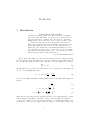
Figure 1 shows a more reliable method of determining altitude. In this method only
the distance d, which is the distance between the two observers making the measurements,
is required. As shown in the figure only the three angles a, b, and c are required. These
angles are the horizontal angles (b and c) between the line connecting the two observers
and the line of the rocket’s flight. The other angle (a) is the vertical angle between the
ground and the rocket’s location. With this method one observer could measure one
angle while the other measures two angles. To make things more robust we will have
both observers measure both the horizontal and vertical angles. This will allow us to
make two altitude calculations with the same set of data – one set where both angles
are used from one observer and the other set where both angles are used from the other
observer. Using these measurements the height of the rocket is
h=
d tan a sin c
sin (b + c)
(14)
[Benson, 2003]. Beware that this formula assumes that all angles are less than 90 degrees.
If your angles are larger, then you will have to make appropriate transformations. When
6
Figure 1: The figure above shows how to determine the altitude of the rocket using
measurements from two observers. This figure is adapted from http://www.grc.nasa.gov/.
deciding where to locate the observers for your launches, note that this method also gives
the best results when the angles are near 45◦ . For this reason, you probably want to
set up your observers so that their locations make a equilateral right triangle, with the
launching pad at the right angle. In order to get angles near 45◦ for the vertical angles,
you will also want the distances from the observers to the launch pad to be roughly the
same as the expected maximum altitude of the rocket.
Note that you should end up with four geometrical estimates of the apogee height
for each launch — two from the simple one-angle method and two from the multi-angle
method.
3
3.1
Data Analysis
Using Mathematica
We will use Mathematica to solve our version of the rocket equation (equation 12). While
performing this analysis you can refer to the sample file performing this calculation in a
simplified case.
The first step in this calculation is to enter your thrust data. Those groups that
determined the thrust curve experimentally should use evaluate their two types of thrust
data, and use whichever type they find appropriate here. Be sure to justify your choice.
In order for Mathematica to be able to use this data you must enter the data into a
table. To do this you will likely want to use the ReadList function. Something along the
lines of
table1 = ReadList[“/home/s03/abstudent/A8 thrust data 00 , {Number, Number, Number, Number}]
should work. The first parameter is the path to the data file, while the other parameters
correspond to the columns in your data file. You may need to edit your file to get it
into a form that Mathematica can deal with. Once you have your data table, you will
7
probably want to use the Interpolation function to make the data into a continuous
function. Be sure to graph your thrust curve over the full time range that you want do
calculations over to be sure that it looks reasonable. Mathematica often puts spikes and
other unphysical features into Interpolating Functions. If you have problems of this sort,
you may have to alter some of the options to Interpolation. For each engine, calculate
the total impulse of the engine and compare it to the expected value.
For the A engine data, consider the drag coefficient, cd to be an unknown and solve
for it by trial and error for each of the three launches that you did with the A engines.
Find the mean and standard deviation for the drag coefficient.
For the B engines, use the drag coefficient that you determined above to find a predicted apogee (including uncertainty) for the B engine flights. Also, re–calculate the drag
coefficient using your B engine apogee data as the known quantities.
1. Compare the prediction of the B engine apogee with your experimental determinations of the apogee. Do they agree? Why or why not?
2. Compare the estimates of the drag coefficient that got for the A engines with the
estimate form the B engines. Do they agree? If not, how could you explain the
discrepancy?
3.2
Using a Spreadsheet
This section will repeat the calculations done for one rocket launch with Mathematica
above using a spreadsheet. Only some groups will do this section, check with your instructor to see if you should. For those of who know how to program, you could also
write a Fortran (or other programming language) program to do this part. Check with
your instructor if you want to write a program to do this part.
Here we will use a spreadsheet (e.g. Gnumeric or Excel) to solve equation 12 using
Euler’s Method [Boyce and DiPrima , 1992, or almost any differential equations textbook].
This method basically involves stepping through the motion of the rocket a small time
step at a time. At each time step the value for the acceleration, velocity, and displacement
is determined from values for the previous time step.
To use this method you will first need to transfer all of the relevant constants, such
as gravitational acceleration, to the spreadsheet. Also, include the value for the drag
coefficient that you determined with Mathematica for this run since for the purposes
of this calculation we will be considering the drag coefficient to be a known quantity.
Then move have to transfer columns (or rows) of data for the thrust as a function of
time and the mass as a function of time. You will probably want to use a Mathematica
command like Table[Cos[i], i, 0, 8, .1] // TableForm, substituting whatever you
called your functions for Cos. These calculations will be performed with time steps of 0.1
s and 0.01 s, so you should prepare data for each case. Also include a column for time
with the difference between consecutive cells following the time step sized listed above.
Next you will make the calculations of acceleration, velocity, and displacement. When
setting up these calculations, for the first cell for each you will want to put the initial value,
which will likely be 0. In the next cell you will set up a formula to calculate the value for
that cell based on previously calculated values. When you are setting up these calculations
that when you place a $ in a cell reference, that reference will remain unchanged when
you copy and paste your formula. So if you are storing your drag coefficient in the cell
B4, you will probably want to refer to it as $B$4.
8
For the acceleration, you should use a formula like
ai+1 =
bvi2
Ti+1
−g−
mi+1
mi+1
(15)
where the indices refer to current and previous time steps. Similarly for velocity and
position we get
vi+1 = vi + ai ∆t
(16)
and
1
xi+1 = xi + vi+1 ∆t + ai+1 (∆t)2
2
Plot the position, speed, and acceleration versus time for both time steps sizes.
(17)
1. How well do these results match your Mathematica results?
2. How do the results compare with different time step sizes?
4
Conclusion
As well as answering the questions listed above, comment on your results.
1. Do your results support the idea of the drag coefficient being a true constant for the
speed regime your rockets were tested in? Why or why not? Make sure to use the
uncertainties that you obtained for the drag coefficients in defending your answer.
2. Describe in more detail than is presented here how the electronic altimeter works.
3. Explain how the geometrical method of determining altitude using two observers
improves accuracy. Hint: there is more to it than simply having better statistics to
average over.
References
Benson,
T.,
A
beginner’s
guide
to
model
http://www.grc.nasa.gov/WWW/K-12/airplane/rkthowhi.html.
rockets,
2003,
Boyce, W. E., and R. C. DiPrima, Elementary Differential Equations and Boundary Value
Problems, John Wiley & Sons, Inc., New York, 1992.
Marion, J. B., and S. T. Thorton, Classical Dynamics of Particle and Systems, Thomson,
Brooks/Cole, Pacific Grove, California, 1995.
Perfect Flite, Alt15/WD User’s Manual , 2003, http://www.perfectflite.com/.
9