Download Chapter 6. THE HIGHER-ORDER METHOD (ILOWHI=1)

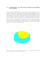
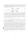
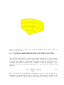
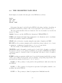
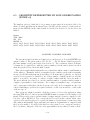
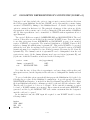
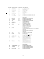
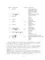
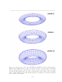
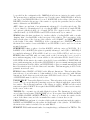
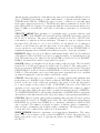
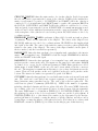
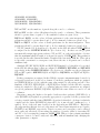
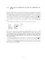
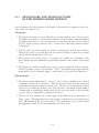
Chapter 6
THE HIGHER-ORDER METHOD
(ILOWHI=1)
The higher-order method which is introduced as an option in Version 6 is fundamentally
different from the low-order panel method described in Chapter 5. The body geometry
can be represented by different techniques including flat panels, B-spline approximations,
geometry models developed in MultiSurf, and explicit analytical formulae. The velocity
potential on the body is represented by B-splines in a continuous manner, and the fluid
velocity on the body can be evaluated by analytical differentiation. In most applications
this provides a more accurate solution, with a smaller number of unknowns, compared to
the low-order method.
This higher-order method is developed from the earlier research code HIPAN, which has
been described in References [18-20].
A brief outline of the method is provided in Sections 6.1-6.3, to give the necessary background for several input parameters which must be specified. This includes the subdivision
of the body surface into patches, the further subdivision of the patches into panels, and
the use of B-splines to develop approximations on these surfaces. It is important to note
in this context that a panel is not restricted to be a flat quadrilateral in physical space,
but can be a general surface in space with continuous curvature to fit the corresponding
portion of the body as precisely as is appropriate.
The number of patches NPATCH is specified in the GDF file. Various options exist to
specify the other input parameters which determine the number or size of the panels, order
of the B-splines, and order of the Gauss quadratures used to integrate over each panel.
Section 6.4 describes the data in the Geometric Data File (GDF) which is common to all
applications of the higher-order method. Sections 6.5-6.8 describe the four different options
for describing the body geometry, and the corresponding inputs. Section 6.9 describes the
procedure for modifying the GEOMXACT subroutine to represent the geometry of userspecified bodies.
If the body has thin elements, there are two possible approaches as in the low-order
method (see Chapter 5). The first is to represent both sides of these elements with patches.
6–1
As a general rule, this approach requires a large number of panel subdivisions of the patches
as the thickness of the elements decreases and thus becomes inefficient. The second is
to reduce the thickness to zero and represent the elements by special ’dipole patches’,
analogous to the thin-wing approximation in lifting-surface theory [21]. Version 6.2 permits
the user to specify a set of dipole patches, as described in Section 6.10.
Section 6.11 describes the optional Spline Control File (SPL) which can be used to define
the orders of the B-Splines, Gauss quadratures, and the numbers of panel subdivisions on
each patch.
The maximum size of the panels (measured in dimensional units) can be specified in
the configuration file, instead of specifying the number of panels on each patch in the SPL
file. This is particularly convenient to achieve a panel size that is commensurate with the
body dimensions and wavelength. Default values of the remaining parameters in the SPL
file (B-spline and Gauss quadrature orders) are assigned automatically, if not input by the
user. Section 6.12 describes this procedure, which permits users to exploit the flexibility
and efficiency of the higher-order method with a minimum of inputs.
6–2
6.1
SUBDIVISION OF THE BODY SURFACE IN PATCHES
AND PANELS
The body surface is first defined by one or more ‘patches’, each of which is a smooth
continuous surface in space. Contiguous patches meet at a common edge, where the coordinates are continuous but the slope may be discontinuous. A simple illustrative example
is provided by the circular cylinder of finite draft shown in Figure 6.1. (The same cylinder
is shown in Figure 5.1 as it would be represented by low-order panels.) Since there are two
planes of geometric symmetry we consider only one quadrant, represented by the shaded
portion of Figure 6.1. Two patches are used, one for the flat horizontal bottom and the
other for the curved cylindrical side. The important properties of the patches are that (a)
the surface is smooth, with continuous coordinates and slope, on each patch, and (b) the
ensemble of all patches represents the complete body surface (or one half or quarter of that
surface, if one or two planes of symmetry exist).
Figure 6.1: Representation of the circular cylinder by two patches on one quadrant, shown by the shaded
portion, with reflections about the two planes of symmetry.
6–3
On each patch a pair of parametric coordinates (u, v) are used to define the position.
The parametric coordinates are normalized so that they vary between ±1 on the patch.
Continuing with the example in Figure 6.1, denoting the cylinder radius R and the draft
D and defining conventional circular cylindrical coordinates (r, θ, z), appropriate choices
for the parametric coordinates are
u=
4θ
− 1,
π
v =1−2
r
R
(6.1)
on the bottom, where 0 ≤ θ ≤ π/2 and 0 ≤ r ≤ R, and
u=
4θ
− 1,
π
v = −2
z
−1
D
(6.2)
on the side, where 0 ≤ θ ≤ π/2 and −D ≤ z ≤ 0. In order to give a consistent definition
for the normal vector we impose the right-hand convention: if the fingers of the right hand
are directed from +u toward +v the thumb should point out of the fluid domain and into
the interior domain of the body. With these definitions the Cartesian coordinates (x, y, z)
of any point on either patch can be expressed in terms of the parametric coordinates (u, v).
More generally, any physically relevant body surface can be represented by an ensemble
of appropriate patches, where the Cartesian coordinates of the points on each patch are
defined by the mapping functions
x = X(u, v),
y = Y (u, v),
z = Z(u, v)
(6.3)
This is the fundamental manner in which the body surface is represented for the higherorder option of WAMIT. Alternative methods for prescribing these mapping functions are
described separately in Sections 6.4-6.7.
In order to provide a systematic procedure for refining the accuracy of approximations
on each patch, a set of smaller surface elements are defined, as described in Section 6.2. For
this purpose each patch is sub-divided in a rectangular mesh, in parametric space. These
elements are referred to as panels. Note that while these panels are flat and rectangular in
parametric space, they are unrestricted in physical space except for the requirement that
they represent a subdivided element of the corresponding patch. Thus, in general, these
panels are curved surfaces in physical space. (In some references, such as [22], panels are
called ‘sub-patches’, or simply ‘patches’). Figure 6.2 shows the example where the side and
bottom of the shaded quadrant in Figure 6.1 are each subdivided into four panels.
In addition to the requirement of geometric continuity within the domain of each patch,
it is also necessary that the hydrodynamic solution should be continuous in the same
domain. For this reason, if discontinous generalized modes are used, as in Test24 described
in Appendix A.24, the modal discontinuities should coincide with boundaries between
adjacent patches.
6–4
Figure 6.2: Subdivision of one quadrant of the cylinder shown in Figure 6,1 into panels. In this case
Nu = Nv = 2 on both patches.
6.2
B-SPLINE REPRESENTATION OF THE SOLUTION
The other important subject to consider is the manner in which the velocity potential is
represented on each patch. Desirable properties of this representation are that it should
be smooth and continuous, corresponding to the physical solution for the fluid flow over
the surface, with control over the accuracy. B-splines are used for this purpose. More
specifically, the velocity potential is represented by a tensor product of B-spline basis
functions
φ(u, v) =
Mv X
Mu
X
φij Ui (u)Vj (v)
(6.4)
j=1 i=1
Here Ui (u) and Vi (v) are the B-spline basis functions of u and v, and Mu and Mv are
the number of basis functions in u and v, respectively. The unknown coefficients φij are
determined ultimately by substituting this representation in the integral equation for the
6–5
potential, as described in Chapter 12. The total number of unknowns on a patch is Mu ×Mv .
In the low order panel method, the accuracy of the numerical solution depends on the
number of panels. (To a lesser extent, the panel arrangement, such as cosine spacing, may
also affect the accuracy of the solution.) In the higher-order method the accuracy depends
on two parameters: the order of the basis functions and their number Mu and Mv . Order
is defined as the degree of the polynomial plus one. For example, a quadratic polynomial
u2 + au + b is of order three. We denote the order of U (u) and V (v) by Ku and Kv ,
respectively. Further information regarding the B-spline basis functions can be found in
Reference [22].
While Ku and Kv are input parameters specified by users, Mu and Mv are not direct
input parameters to WAMIT. Instead, users may specify the number of panel subdivisions
on each patch, Nu and Nv . (In standard B-spline terminology, these correspond to knots.)
Alternatively, users can specify the desired size of each panel in physical space, and the
program will automatically assign the corresponding inputs Nu and Nv on each patch to
achieve this objective.
The relations between the number of basis functions and the number of panels are as
follows:
(6.5)
Mu = Nu + Ku − 1 Mv = Nv + Kv − 1
Since Ku = Kv = 1 in the low-order panel method, the number of unknowns is the same
as the number of panels. Chapter 6 of [18] contains examples showing how the accuracy
of the solution depends on K and N for various geometries.
6–6
6.3
ORDER OF GAUSS QUADRATURES
Another topic which must be considered is the integration over patch surfaces. Since
the Galerkin method is used to solve the boundary integral equation, as described in
Chapter 12, this integration is carried out first with respect to the source point, and then
with respect to the field point. These are referred to respectively as the inner and outer
integrations which are carried out in parametric space. For this purpose, each patch is
sub-divided into Nu × Nv panels, and Gauss-Legendre quadrature is applied on each panel.
The orders of the Gauss quadratures are specified by input parameters. Experience with a
variety of applications has shown that it is sufficient to set the order of the outer integrals
with respect to (u, v) equal to (Ku , Kv ) and the order of the inner integrals equal to
(Ku + 1, Kv + 1).
6–7
6.4
THE GEOMETRIC DATA FILE
In the higher-order method the first part of the GDF file is as follows:
header
ULEN GRAV
ISX ISY
NPATCH IGDEF
Subsequent data may be included in the GDF file after these four lines, depending on
the manner in which the geometry of the body is represented. (See Sections 6.5-6.8.)
The data on the first three lines are identical to the low-order method as described in
Section 5.1. Thus:
‘header’ denotes a one-line ASCII header dimensioned CHARACTER∗72.
ULEN is the dimensional length characterizing the body dimensions, used to nondimensionalize the quantities output from WAMIT.
GRAV is the acceleration of gravity, using the same units of length as in ULEN.
ISX, ISY are the geometry symmetry indices which have integer values 0, +1 to denote
no symmetry, or symmetry about the plane x = 0 or y = 0 respectively.
The data on line 4 of the GDF file are defined as follows:
NPATCH is equal to the number of patches used to describe the body surface, as explained
in Section 6.1. If one or two planes of symmetry are specified, NPATCH is the number
of patches required to discretize a half or one quadrant of the whole of the body surface,
respectively.
IGDEF is an integer parameter which is used to specify the manner in which the geometry
of the body is defined. Four specific cases are relevant, corresponding respectively to the
representations explained in Sections 6.5, 6.6, 6.7 and 6.8:
IGDEF = 0: The geometry of each patch is a flat quadrilateral, with vertices listed in
the GDF file.
IGDEF = 1: The geometry of each patch is represented by B-splines, with the corresponding data in the GDF file.
IGDEF = 2: The geometry is defined by inputs from a MultiSurf .ms2 file.
6–8
IGDEF < 0 or > 2: The geometry of each patch is represented explicitly by a special
subroutine, with optional data in the GDF file
6–9
6.5
GEOMETRY REPRESENTED BY LOW-ORDER PANELS
(IGDEF=0)
The simplest option to define the body geometry is appropriate if each patch of the body
surface is a flat quadrilateral in physical space. In this case the vertices of each patch are
input via the GDF file in the same format as described in Section 5.1 for the low-order
method:
header
ULEN GRAV
ISX ISY
NPATCH 0
X1(1) Y1(1) Z1(1) X2(1) Y2(1) Z2(1) X3(1) Y3(1) Z3(1) X4(1) Y4(1) Z4(1)
X1(2) Y1(2) Z1(2) X2(2) Y2(2) Z2(2) X3(2) Y3(2) Z3(2) X4(2) Y4(2) Z4(2)
.
.
.
.
.
. . . . .
.
. . . . X4(NPATCH) Y4(NPATCH) Z4(NPATCH)
The data in the first four lines are defined above, in Section 6.4. Note that IGDEF=0 is
assigned on line 4. The patch vertices (X1, Y 1, Z1, ... , X4, Y 4, Z4) are defined in precisely
the same manner as the panel vertices in Section 5.1. The convention defined in Figure
5-1 must also be applied here, with the vertices numbered in the anti-clockwise direction
when the patch is viewed from the fluid domain.
This option is particularly useful in the case of structures which consist of a small number
of flat surfaces. Examples include rectangular barges, similar vessels with rectangular
moonpools, the Hibernia platform (a star-shaped bottom-mounted cylinder), etc. In such
cases it is not necessary or desirable to use a large number of small patches on each flat
surface, as would be necessary to achieve accurate results with the low-order method.
The most efficient procedure is to use the smallest number of patches which permits a
complete representation of the structure. For a simple rectangular barge, one quadrant
can be represented with three patches (bottom, side, end). If a rectangular moonpool is
centered amidships, 6 patches are required with two on the bottom and two on the walls
of the moonpool.
This option also might be useful to check the accuracy of a low-order application, using
the same GDF file for both (except that IGDEF=0 must be assigned for the higher-order
input). This provides a more general scheme for improving the accuracy compared to the
low-order option IQUAD=1. Two caveats should be noted in this context. First, since
each low-order panel is replaced by a patch, the number of patches may be quite large; this
will result in substantially longer run times and memory requirements as compared with
the low-order method. Secondly, if the flat low-order panels do not correspond exactly to
the body surface, this part of the low-order approximation is not refined by such a check.
6–10
6.6
GEOMETRY REPRESENTED BY B-SPLINES (IGDEF=1)
The most general approach to represent the geometry in the higher-order method is the
same as that which was first developed in [18,19]. In this approach each patch of the
body is represented by B-splines, in an analogous manner to the representation of the
velocity potential (Section 6.2). The panel subdivision (knot vector) and the order of
the B-splines can be assigned independently between the geometry and the potential. If
the subdivisions and orders are the same, this is analogous to the isoparametric approach
in finite-element analysis. In V6.2, the domain of the parameters of the B-SPLINES
representing the geometry is no longer limited to (−1, 1). Arbitrary limits can be used and
they are normalized to (−1, 1) in the program.
More specifically, the mapping function X = (X, Y, Z) defined by Equation (6.3) is
represented on each patch in the tensor-product form
(g)
X(u, v) =
(g)
M
M
v
u
X
X
Xij Ui (u)Vj (v)
(6.6)
j=1 i=1
Here Ui (u) and Vi (v) are the B-spline basis functions of u and v, and Mu(g) and Mv(g) are
the number of basis functions in u and v, respectively. (The superscripts are used to distinguish these geometric parameters from the corresponding parameters used to represent
the potential in Section 6.2.) As in (6.5),
Mu(g) = Nu(g) + Ku(g) − 1 Mv(g) = Nv(g) + Kv(g) − 1
(6.7)
where Ku(g) and Kv(g) are the orders of the respective B-splines. These parameters, and the
values of the unknown coefficients Xij , are assigned for each patch in the GDF file.
The format of the GDF file is as follows:
header
ULEN GRAV
ISX ISY
NPATCH 1
NUG(1) NVG(1)
KUG(1) KVG(1)
VKNTUG(1,1) ... VKNTUG(NUA(1),1)
VKNTVG(1,1) ... VKNTVG(NVA(1),1)
XCOEF(1,1) XCOEF(2,1) XCOEF(3,1)
XCOEF(1,2) XCOEF(2,2) XCOEF(3,2)
·
·
·
XCOEF(1,NB(1)) XCOEF(2,NB(1)) XCOEF(3,NB(1))
·
6–11
·
·
NUG(NPATCH) NVG(NPATCH)
KUG(NPATCH) KVG(NPATCH)
VKNTUG(1,NPATCH) ... VKNTUG(NUA(NPATCH),NPATCH)
VKNTVG(1,NPATCH) ... VKNTVG(NVA(NPATCH),NPATCH)
XCOEF(1,1) XCOEF(2,1) XCOEF(3,1)
XCOEF(1,2) XCOEF(2,2) XCOEF(3,2)
·
·
·
XCOEF(1,NB(NPATCH)) XCOEF(2,NB(NPATCH)) XCOEF(3,NB(NPATCH))
Here IGDEF=1 is assigned on line 4 to specify the B-spline representation of the geometry.
NUG(I) and NVG(I) are the numbers of panel subdivisions of the u and v coordinates
on I-th patch.
KUG(I) and KVG(I) are the orders of B-splines
VKNTUG(J,I) is the B-spline knot vector in u on patch I. J=1,2,...NUA(I)
NUA(I)=NUG(I)+2*KUG(I)-1.
VKNTVG(J,I) is the B-spline knot vector in v on patch I. J=1,2,...NVA(I)
NVA(I)=NVG(I)+2*KVG(I)-1.
XCOEF(1,K)) XCOEF(2,K) XCOEF(3,K) are the components of the vector coefficient Xij in (6.6). These are defined in terms of the single array index K, where
K=1,2,...,NB(I). Here NB(I) is the total number of coefficients on patch I, given by the
relation NB(I)=(NUG(I)+KUG(I)-1)×(NVG(I)+KVG(I)-1).
TEST11 (Appendix, Section A.11) is an example of this type of GDF input file.
6–12
6.7
GEOMETRY REPRESENTED BY MULTISURF (IGDEF=2)
Versions 6.2 and later include the option to import .ms2 geometry database files from
the CAD program MultiSurf directly into WAMIT, and to represent the geometry during
execution of WAMIT by linking to the MultiSurf kernel. A detailed description of this
option is contained in Reference 24. The principal advantages of this option are (a) the
representation of the geometry can be developed using the CAD environment of MultiSurf,
and (b) this representation can be transferred to WAMIT without significant effort or
approximations.
Two special .dll files are required: RGKERNEL.DLL and RG2WAMIT.DLL. The ‘real’
versions of these files are not included in the standard WAMIT license. Users who intend
to use this option may license RGKERNEL and RG2WAMIT as part of an extended
version of WAMIT, or separately. The standard distribution of WAMIT Version 6.2PC
includes a ‘dummy’ file with the name ”rg2wamit.dll”. This enables WAMIT to be executed
without the ‘real’ files. As explained in Section 2.1, the PC-executable version of WAMIT
(wamit.exe) must be accompanied by four .dll files (geomxact.dll, newmodes.dll, dforrt.dll,
rg2wamit.dll). The dummy version of rg2wamit.dll can be distinguished from the real
version in two ways: (a) the dummy filename uses lower-case letters (rg2wamit.dll), and
(b) the size of this file is smaller, as indicated in the following table:
version
name
dummy
real
rg2wamit.dll
RG2WAMIT.DLL
size (approximate)
30Kb
94Kb
Note that the size of these files is approximate, and may change with updates and
subsequent versions, but the disparity in size will serve to distinguish the dummy and real
files.
To proceed with this option a user should first prepare the MultiSurf model for the body
following the procedure in the MultiSurf documentation. A special appendix ‘Using the
WAMIT-RGKernel Interface’ is included in this User Manual (Appendix C). The output
file from MultiSurf will include a filename specified by the user and the extension ‘.ms2’.
This file will be referred to below as ‘body.ms2’. If the .ms2 file is missing or cannot
be found, a WAMIT runtime error message ‘Error return from subroutine RGKINIT’ is
generated, and the log file ‘RGKLOG.TXT’ will contain a statement that the designated
.ms2 file could not be opened.
In its simplest form, the GDF input file required to run WAMIT should be in the
following format:
header
ULEN GRAV
ISX ISY
NPATCH
2
6–13
3
(path)body.ms2
*
0 0 0
The first four lines are explained in Section 6.4. IGDEF=2 is assigned by the second
integer on line 4. Line 5 contains an integer specifying the number of subsequent lines to
be read from the .gdf file. Line 6 contains the name of the .ms2 file, and may include the
optional path if this file is in a different directory (folder). The asterisk (∗) on line 7 is
a default specifier to indicate that all visible surfaces in the .ms2 file are to be included;
alternatively if only a subset of these surfaces are submerged these may be designated by
following the instructions in Appendix C. Line 8 includes three integer parameters with
default values zero, which may be used to control the accuracy of the geometry evaluation
in RGKernel, and also to modify the convention regarding the direction of the unit normal.
Further information is contained in Appendix C. TEST11C and TEST20 in Appendix A are
examples showing typical WAMIT runs for a circular cylinder and for a barge. Additional
examples are included in Reference 24.
Starting with Version 6.4, NPATCH can be specified as 0; use of this option is recommended, to avoid errors in counting surfaces or patches. In this case the number of patches
is evaluated from the MultiSurf model, and the user does not need to input NPATCH
separately. If NPATCH¿0 is input by the user, the number of MultiSurf surf aces used in
the solution will be limited to NPATCH; thus input files for earlier versions of WAMIT
can still be used without modification.
Starting with Version 6.4 dipole patches (thin submerged elements) can be defined in
the MultiSurf model, as explained in Appendix C. As noted in Section 6.10, the dipole
patches should only be identified in the MultiSurf model and not in the GDF file when
IGDEF=2.
Starting with Version 6.4 a low-order GDF file can be generated and output, directly
from the MultiSurf model, during the WAMIT run, as explained in Appendix C.
A pre-processor utility GDF2MS2.EXE has been developed by AeroHydro Inc.1 to
convert low-order WAMIT .gdf input files to .ms2 geometry database files for MultiSurf.
Its results depend on the organization and content of the .gdf file. In general this utility
will create correctly dimensioned points for building a surface model in MultiSurf; and if
the .gdf file is suitably structured it is possible to create appropriate surface patches for
higher-order analysis with the IGDEF=2 option.
1 AeroHydro,
Inc., 54 Herrick Rd., Southwest Harbor, Maine 04679 USA 207-244-4100 (www.aerohydro.com)
6–14
6.8
ANALYTIC REPRESENTATION OF THE GEOMETRY
This option can be used in cases where the geometry of the body can be defined explicitly,
with the fundamental advantage that the definition of the body geometry is exact and that
the only numerical approximation which remains is in the representation of the velocity
potential. Further details and examples based on this method are contained in Reference
25. The domain of parameters must be (-1.,1) in analytic representation.
The formulae required to define the geometry must be coded in FORTRAN, in the file
GEOMXACT.F. This file can be compiled separately as a .dll file and linked with WAMIT
at runtime. This special arrangement makes it possible for users of the PC executable
code to modify GEOMXACT for their own particular applications. Another feature of
this option is the possibility to input relevant body dimensions in the GDF file. Thus the
body dimensions can be changed without modification of the code.
In the version of GEOMXACT.F and GEOMXACT.DLL as supplied with the WAMIT
software, there are several subroutines to produce various generic body shapes as listed
in the table below. Most of these subroutines are illustrated in the higher-order test
runs described in Appendix A. The dimensions of these generic bodies can be modified
by introducing appropriate data in the GDF file. Thus there is a variety of possibilities
for exploiting this option with or without special programming efforts. Several different
subroutines can be collected in a library, and identified with specific reserved values of
the index IGDEF which is input in the GDF file. The WAMIT software includes the
FORTRAN library file GEOMXACT.F, where several examples of these subroutines are
included. Note that IGDEF=0 or 1 are reserved for the options described in Sections 6.5
and 6.6, and thus IGDEF≥ 2 or IGDEF≤ −1 are appropriate values to select for the
analytic representation option. In the WAMIT software package as distributed, several
negative values IGDEF≤ −1 have been used for the test runs, and for other pertinent
examples which may be useful. Thus it is recommended that any new additions to this
library developed by users should be identified with positive values IGDEF≥ 2.
Continuing with the example of the circular cylinder shown in Figures 6.1 and 6.2, the
subroutine CIRCYL can be used without modification. CIRCYL is included in the source
file GEOMXACT.F and selected by specifying IGDEF=-1. The relevant dimensions are
the radius and draft (and also ULEN and GRAV), which are specified in the GDF file in
the following format:
header
ULEN GRAV
1 1
2
-1
2
RADIUS DRAFT
INONUMAP
6–15
Here the symmetry indices ISX=1 and ISY=1 have been assigned, as well as the parameters
NPATCH=2 and IGDEF=-1. The number 2 on line 5 indicates that two lines follow in the
file to be read as input data. In addition to the dimensions of the cylinder, the parameter
INONUMAP is used in subroutine CIRCYL to specify either uniform (INONUMAP=0)
or nonuniform (INONUMAP=1) mapping between the parametric coordinates (U,V) and
the Cartesian coordinates (X,Y,Z).
Uniform mapping uses linear functions to transform V to the vertical coordinate on
the side, and to the radial coordinate on the bottom (and interior free surface). When
the nonuniform mapping option is selected the vertical coordinate on the side is a cubic
polynomial in V, and the radial coordinate on the other patches is a quadratic polynomial
in V, such that the first derivatives vanish at the corner and at the intersection of the
side and free surface. This nonuniform mapping is analogous to the use of ‘cosine spacing’
in the low-order panel method, to achieve a finer discretization of the solution near these
boundaries. The motivation for using the nonuniform mapping option is discussed in
Appendix A.11, where both options are compared, and in more detail in Reference 25.
The code in the subroutine CIRCCYL may be used as a guide for other geometries where
nonuniform mapping is desirable.
Before using this GDF file the user should assign appropriate values for the parameters
ULEN, GRAV, RADIUS, DRAFT, INONUMAP, and an appropriate header. As noted in
Section 3.7, this data must be contained within columns 1-80 of the GDF file.
In the normal case described above, NPATCH=2, corresponding to the side and bottom
of the cylinder. Two other situations exist where the same subroutine can be used: (1)
for a bottom-mounted cylinder NPATCH=1 and DRAFT is assigned with the same value
as the fluid depth HBOT, and (2) if NPATCH=3 the interior free surface is included to
permit the removal of irregular-frequency effects (IRR=1) as described in Chapter 9. The
restriction DRAFT<HBOT must be imposed if NPATCH>1. Figure 6.3 illustrates the
patch numbering to achieve this flexibility.
6–16
Figure 6.3: One quadrant of the cylinder shown in Figure 6.1 showing the patch numbering system which
permits using the subroutine CIRCYL with NPATCH=1 (bottom-mounted caisson), NPATCH=2 (floating
cylinder of finite draft), or NPATCH=3 (floating cylinder with a patch on the interior free surface to remove
irregular-frequency effects). The view is from above the free surface, looking toward the interior of the
cylinder.
Other subroutines are also included in GEOMXACT.F to define a variety of bodies, in
all cases with IGDEF<0 so that positive values of IGDEF>2 will be reserved for users. 32
body subroutines are included in the standard release of GEOMXACT.F and GEOMXACT.DLL, as listed in the table below and explained in detail here. Several of these are
used for the higher-order Test Runs described in Appendix A. In addition there are 4
control-surface subroutines in the standard release of GEOMXACT, which are described
in Chapter 14. Several additional subroutines are also included in an extended version of
GEOMXACT for possible use by users, and in a library which can be downloaded from
www.wamit.com. The details of these other subroutines are explained in comments which
are inserted in the source code of each subroutine in the file GEOMXACT LONG.F.
The following table lists the 32 body subroutines, which are described in more detail
below:
6–17
IGDEF SUBROUTINE
NPATCH
GDF INPUTS
RADIUS,DRAFT
INONUMAP
A,B,DRAFT
RADIUS
INONUMAP
A,B,C
HALFLEN,HALFBEAM,DRAFT
HALFLEN,HALFBEAM,DRAFT
XMP,YMP
RADIUS,DRAFT,RADMP
RCIRC,RAXIS,ZAXIS
RADIUS,DRAFT,HSPACE
WIDTH,HEIGHT
XL,Y1,Y2,Z1,Z2
DCOL,RCOL,NCOL
XBOW,XMID,XAFT
HBEAM,HTRANSOM
DRAFT,DTRANSOM
RADIUS DRAFT
WIDTH THICKNESS TWIST NSTRAKE
IRRFRQ
IMOONPOOL, RADIUSMP
IMPGEN
RADIUS, DCYL, DTAIL
RAD1,RAD2
DRAFT,SKIRT HEIGHT
RADIUS,X0,Y0,Z0
XBOW,XMID,XAFT
HBEAM,HTRANSOM
DRAFT,DTRANSOM
INONUMAP
XBOW,XMID,XAFT
HBEAM,HTRANSOM
DRAFT,DTRANSOM
INONUMAP
RCIRC,RAXIS,DRAFT
RCIRC1,RAXIS1,DRAFT1
RCIRC2,RAXIS2,DRAFT2
RADIUS,HALFLEN
-1
CIRCCYL
1,2,3
-2
-3
ELLIPCYL
SPHERE
1,2,3
1,2
-4
-5
-6
ELLIPSOID
BARGE
BARGEMP
1,2
1,2,3,4
6,7
-7
-8
-9
CYLMP
TORUS
TLP
3,4
1,2
11,12
-10
SEMISUB
-11
FPSO
-12
SPAR
-13
-14
AUV
SPAR2
2,3
3,4,5
-15
-16
SPHERXYZ
FPSO2
1
7,10
-17
FPSO12
7,10
-18
-19
TORUS ELLIP
TORUS2
1,2
2
-20
CIRCCYLH
2,3
4,6
6–18
IGDEF SUBROUTINE
NPATCH
-21
FPSOINT
-
-22
CIRCCYL ARRAY
-23
ELLIPINT
-24
GAPLID
1
-25
CYLFIN
2,3,4
-26
CYLFIN4
4,6,9
-27
-28
SKEW SPHERE
CIRCCYL NOSYM
1,2
1,2,3
-29
ELLIPSOID NOSYM TANK
-30
-31
-32
BARGE INT
BARGENUC
CCYLHSP
-
-
3
12,13
GDF INPUTS
XBOW,XMID,XAFT
HBEAM,HTRANSOM
DRAFT,DTRANSOM
INONUMAP,NTANKS
XVER
RADIUS,DRAFT,ASPACE
NX,NY,INONUMAP
A,B,C
NTANKS
XVER
X1,X2,GAP
INONUMAP
RADIUS,DRAFT
WIDTH
INONUMAP
RADIUS,DRAFT
WIDTH
INONUMAP
RADIUS,SKEW
RADIUS,DRAFT
INONUMAP
XS,YS,ZS
A,B,C
XS,YS,ZS
XL,XB,XD,SL,SB,SD
HALFLEN,HALFBEAM,DRAFT
HALFLEN,HALFBEAM,DRAFT,STRIP
NSEG
RADIUS
XSEG
The last column indicates the dimensions and other input parameters to be included
in the GDF file. Where two or more lines of inputs are shown in the table the GDF file
should follow the same format, as illustrated in the test runs.
Brief descriptions of each subroutine are given below. More specific information is
included in the comments of each subroutine. These bodies can be combined for multiplebody analysis, as described in Chapter 7, without modifications of the subroutines.
CIRCCYL defines a circular cylinder as explained above.
ELLIPCYL defines an elliptical cylinder with semi-axes A,B. If A=B=RADIUS the results are identical to using CIRCCYL. The options NPATCH=1 (bottom mounted) and
NPATCH=3 (IRR=1) are the same as for CIRCCYL. The semi-axes A and B coincide
with the x− and y−axis of the body coordinate system, respectively.
6–19
SPHERE defines a floating hemisphere, with one patch on the body surface. If NPATCH=2
the interior free surface is included for use with the irregular-frequency option (IRR=1).
The optional parameter INONUMAP can be included to specify either uniform (INONUMAP=0) or nonuniform (INONUMAP=1) mapping. Uniform mapping is the default,
and it is not necessary to include INONUMAP in this case. If INONUMAP=1 is specified
the mapping in the azimuthal direction on the hemisphere is quadratic, to give a finer discretization close to the waterline. Similarly, if IRR=1, INONUMAP=1 defines a quadratic
radial mapping on the interior free surface with finer discretization close to the waterline
so that the interior and exterior discretizations are similar at this point.
ELLIPSOID defines an ellipsoid with semi-axes A,B,C, floating with its center in the
plane of the free surface. (C is equal to the draft.) If A=B=C=RADIUS the results are
identical to using SPHERE. The semi-axes A, B and C coincide with the x−, y− and
z−axis of the body coordinate system, respectively.
BARGE defines a rectangular barge with length equal to 2×HALFLEN and beam equal
to 2×HALFBEAM. In the simplest case NPATCH=3 patches are used to represent the
end, side, and bottom on one quadrant. If NPATCH=1 and DRAFT=0.0 only the bottom is represented, corresponding to a rectangular lid in the free surface. If NPATCH=2
and DRAFT=HBOT the barge is a bottom-mounted rectangular caisson. If NPATCH=4
the interior free surface is included for use with the irregular-frequency option (IRR=1).
The longitudinal and transverse directions coincide with the x− and y−axis of the body
coordinate system, respectively.
BARGEMP defines a rectangular barge with a rectangular moonpool at its center. The
moonpool is bounded by vertical walls x = ±XMP and y = ±YMP. Other dimensions are
the same as for BARGE. In the normal case, NPATCH=6, separate patches are on the end
and side, two patches on the bottom, and two patches for the moonpool walls. Optionally,
if NPATCH=7, the moonpool free surface is represented by an additional patch; this is an
alternate scheme for the analysis of moonpools, using generalized modes to describe the
free surface so that resonant modes can be damped. TEST17B illustrates this scheme.
The longitudinal and transverse directions coincide with the x− and y−axis of the body
coordinate system, respectively.
CYLMP defines a spar-type structure consisting of a circular cylinder with a concentric
moonpool of constant radius RADMP. In the normal case, NPATCH=3, separate patches
are on the outer side of the cylinder, on the bottom, and on the interior wall of the moonpool. Optionally, if NPATCH=4, the moonpool free surface is represented by an additional
patch; this is an alternate scheme for the analysis of moonpools, using generalized modes
to describe the free surface so that resonant modes can be damped. TEST17B gives a
description of this scheme.
TORUS defines a floating or submerged torus, as illustrated in Figure 6.4. The sections
of the torus are circles of radius RCIRC, with their axes on a circle of radius RAXIS in
the horizontal plane z =ZAXIS. If -RCIRC<ZAZIS<RCIRC the torus is floating, and if
ZAXIS<-RAXIS the torus is submerged. One quadrant of the surface is represented by
one patch. If the torus is floating, and NPATCH=2, the free surface inside the ”moonpool”
is represented by an additional patch, as in CYLMP.
6–20
Figure 6.4: Perspective views of the torus, with RCIRC=20, RAXIS=60, and three different values of
ZAXIS as shown. ZAXIS>0 in the top figure corresponds to the axis above the free surface. In the middle
figure the axis is in the plane of the free surface, and the sections are semi-circles. In these two figures
the torus is floating, with the upper edges of the body in the plane of the free surface. The bottom figure
shows a complete submerged torus. The dark lines indicate the boundaries between adjacent quadrants,
with one patch on each quadrant.
6–21
TLP defines a generic tension-leg platform (TLP) with four circular columns connected by
rectangular pontoons. The bottom surfaces of the columns and pontoons are at the same
draft and the columns are equally spaced in a square array. The quadrant is defined to
include one column and half of the adjoining pontoons. The column radius RADIUS and
draft DRAFT and a half of the horizontal spacing between the axes of adjacent columns
HSPACE are specified on one line of the GDF file. The pontoon width WIDTH and height
HEIGHT are specified on a separate line. The width of the pontoons is restricted √
so that
they do not intersect off the columns. In the special case WIDTH=RADIUS× 2 the
pontoon corners coincide on the column and NPATCH=11. This includes eight patches on
the top, sides, and bottom of the pontoons, one patch on the column above the pontoons,
one patch on the column outside the √
pontoons, and one patch on the column bottom. In
the general case WIDTH<RADIUS× 2, NPATCH=12 with the 12th patch on the column
between the inside corners of adjacent pontoons. This case is illustrated in the test run
TEST14.
SEMISUB defines a generic semi-submersible with two rectangular pontoons and NCOL
equally-spaced circular columns on each pontoon. The pontoon dimensions include the
total length XL, transverse coordinates of the inner/outer pontoon sides Y1, Y2, and
vertical coordinates of the bottom and top horizontal surfaces Z1, Z2. Note that 0<Y1<Y2
and Z1<Z2≤0. (The overall beam is equal to 2×Y2 and the draft is equal to -Z1.) The
pontoon ends are semi-circular. NPATCH depends on the number of columns, and their
spacing, as explained in the subroutine header. If Z2=0 and NPATCH=2 the pontoons
intersect the free surface. The test run TEST15 illustrates the use of this subroutine for a
semi-sub with submerged pontoons and five columns on each pontoon.
FPSO defines a monohull ship with a form representative of the ‘Floating Production
Ship Offloading’ type. ( A perspective view of this vessel is shown on the cover page.) The
hull consists of three portions: (1) an elliptical bow with a flat horizontal bottom, vertical
sides, and semi-elliptical waterlines, (2) a rectangular mid-body with a flat horizontal
bottom, vertical sides, and constant beam, and (3) a prismatic stern with rectangular
sections. The dimensions XBOW, XMID, XAFT define the longitudinal extent of these
three portions. The total length of the vessel is equal to (XBOW+XMID+XAFT), and
the origin of the coordinate system is defined at the midship section, half-way between
the bow and stern. The dimensions include the half-beam HBEAM, half-width of the
transom HTRANSOM, maximum draft DRAFT, and transom draft DTRANSOM. In the
general case NPATCH=6, with the patch indices 1-6 corresponding respectively to (1)
the horizontal bottom, (2) the vertical portion of the bow, (3) sides of the mid-body, (4)
transom, (5) sloping bottom on the prismatic stern, and (6) sloping side on the prismatic
stern. The prismatic stern portion can be omitted by setting NPATCH=4, XAFT=0.0,
HTRANSOM=HBEAM, and DTRANSOM=DRAFT.
SPAR defines a spar with strakes and with an optional moonpool. The number of patches
varys depending on the optional configuration. RADIUS is the radius of the spar. DRAFT
is the vertical length. WIDTH and THICKNESS are the width and thickness of the strakes.
Helical form of strakes can be generated by specifying nonzero TWIST which represents
the number of revolutions from top to bottom in the counter-clockwise direction viewed
from the top. IRRFRQ=1 includes the interior free surface and, in this case, IRR=1 should
6–22
be specified in the configuration file. IRRFRQ=0 indicates no interior free suface patch.
The spar may have a uniform circular moonpool at the center. IMOONPOOL=1 includes
a moonpool and IMOONPOOL=0 does not. RADIUSMP is the radius of the moonpool.
IMPGEN=1 includes the moonpool free surface to specify the generalized modes on that
surface. Otherwise set IMPGEN=0.
AUV defines one quadrant of an axisymmetric submerged body with vertical axis. The
body is defined by a hemispherical bow of radius RADIUS, conical tail of length DTAIL,
and optional cylindrical midbody of length DCYL. The origin is at the center of the
cylindrical midbody. If NPATCH=2 and DCYL=0.0 the midbody is omitted.
SPAR2 defines the first quadrant of a circular cylinder of radius RAD1 with a circular
damping ‘skirt’ of radius RAD2 on the lower part of the cylinder. The lower surface of the
skirt is in the plane of the bottom of the cylinder, at Z=-DRAFT, and SKIRT HEIGHT
is the height of the skirt. NPATCH=4 is the conventional case, NPATCH=5 includes
the interior free surface for use with IRR=1, and NPATCH=3 can be used for a bottommounted structure.
SPHERXYZ defines a sphere of radius RADIUS, with its center at X0,Y0,Z0. If (RADIUS < Z0 < RADIUS) the sphere is partially submerged, and if (Z0 < -RADIUS) it
is completely submerged. If X0=0 ISX=1, and vice versa. If Y0=0 ISY=1, and vice versa.
FPSO2 defines an FPSO with one extra patch on the bottom in the bow to provide a
more uniform mapping of the bottom relative to the subroutine FPSO described above.
If NPATCH=10 the interior free surface is included for use with IRR=1. INONUMAP=0
gives a uniform mapping on all patches; INONUMAP=1 gives a nonuniform mapping with
finer discretization near the chines; and INONUMAP=2 gives a nonuniform mapping with
finer discretization near both the chines and waterline. Uniform mapping is used for the
prismatic stern in all cases.
FPSO12 defines NBODY=2 FPSO’S with different dimensions. This subroutine illustrates the use of one subroutine to define multiple bodies of the same type with different
dimensions. In all other respects it is the same as FPSO2 described above. The same value
of INONUMAP must be used for both bodies.
TORUS ELLIP Torus with elliptical sections. This subroutine is the same as TORUS,
described above, except that the generating sections are elliptical with their centers in the
free surface. The horizontal semi-axis of the ellipses is equal to RCIRC and the vertical
semi-axis is equal to DRAFT. It is required that RAXIS>RCIRC, i.e. there is a free surface
in the center of the torus.
TORUS2 Two concentric toroids with elliptical sections. The dimensions of each toroid
are as defined in subroutine TORUS ELLIP above. It is required that RAXIS1>RCIRC1
and RAXIS2>(RAXIS1+RCIRC1+RCIRC2), i.e. there is a circular free surface in the
center of the inner torus, and also an annular free surface between the toroids.
CIRCCYLH First quadrant of a circular cylinder with a horizontal axis in the free surface.
RADIUS and HALFLEN are the radius and half-length of the cylinder. If NPATCH=3
the interior free surface is included for use with IRR=1.
FPSOINT FPSO with internal tanks of rectangular shape, as illustrated in TEST22. The
6–23
dimensions and representation of the hull are the same as in subroutine FPSO2 described
above. NTANKS is the number of tanks, which must be consistent with the inputs for
NPTANK in the CFG file. XVER is the array of vertex coordinates for each tank, input
in the same format as in Section 6.5. The FPSO and tanks are symmetric about the Y=0
plane (ISX=0,ISY=1). Patches 1-7 represent the hull and 8-10 represent the interior free
surface if IRR=1, as in FPSO2. One half of each tank is represented by 4 additional
patches.
CIRCCYL ARRAY First quadrant of a rectangular array of circular cylinders, with
radius RADIUS, draft DRAFT, and horizontal spacing ASPACE between the centers in
the X- and Y- directions. The array is symmetric about X=0 and Y=0. NX*NY is the
total number of cylinders in all four quadrants. NX must be even (no cylinders are in
the plane X=0). NY may be odd or even. If NY is odd the middle row of cylinders is
centered on the X-axis and only the upper half of each cylinder is represented. There
are two patches for each cylinder, representing the side and bottom. If INONUMAP=1
nonuniform mapping is used with finer discretization near the corners and waterlines.
ELLIPINT defines one side of an ellipsoid with internal tanks. A,B,C are the semi-axes
of the ellipsoid. ISX=0 and ISY=1 are used to permit the tanks to be assymmetrical about
X=0. The tank vertices are defined by the array XVER as described above for FPSOINT.
If IRR=1 the internal free surface is represented by patch 2.
GAPLID defines a rectangular ‘lid’ in the free surface with one patch. The lid extends
from X=X1 to X=X2 and between Y=-GAP/2 and Y=+GAP/2. The entire surface of
the lid is represented (ISX=ISY=0). Nonuniform discretization is used in the X-direction
if INONUMAP=1, in the Y-direction if INONUMAP=2, and in both directions if INONUMAP=3. This subroutine can be used with appropriate generalized modes to establish
an artifical damping lid on the free surface between two vessels.
CYLFIN defines the first 1 or 2 quadrants of a circular cylinder with symmetric fins
in the plane x=0. RADIUS is the cylinder radius and WIDTH is the width of the fins.
Patch 1 is the side of the cylinder in quadrant 1 and patch 2 is the fin (represented
by a dipole patch) on the positive Y-axis. If NPATCH=3 the side of the cylinder in
quadrant 2 is also represented. If RADIUS=0 and NPATCH=1 the cylinder is omitted
and the subroutine defines the upper half of a single fin extending from Y=-WIDTH to
Y=+WIDTH. INONUMAP is optional with default value 0. If INONUMAP=1 is input the
discretization on the fins is finer near the outer ends, using a cosine-spacing transformation.
CYLFIN4 defines a circular cylinder with 4 symmetric fins represented by dipole patches
in the planes X=0 and Y=0. DRAFT is the draft. The other dimensions and parameter
INONUMAP are as defined for CYLFIN above. Arbitrary combinations of ISX and ISY
can be specified. The number of patches is equal to 4 with two planes of symmetry, 6
with one plane of symmetry, and 9 with no planes of symmetry. The last patch is on the
bottom, and can be omitted if the cylinder is bottom-mounted.
SKEW SPHERE defines two quadrants of a floating skewed hemisphere. The centerplane of the body is inclined, at the position X=SKEW*Z. Patch 1 represents the body
surface and patch 2 can be used to represent the interior free surface if IRR=1. ISX=0
and ISY=1.
6–24
CIRCCYL NOSYM defines the entire surface of a circular cylinder. Patch 1 represents
the side and patch 2 represents the bottom of the cylinder. If IRR=1 the internal free
surface is represented by patch 3. If NPATCH=1 and DRAFT≥1.E-8 the cylinder is
considered to be bottom-mounted and DRAFT must be equal to the parameter HBOT in
the POT file. If NPATCH=1 and DRAFT<1.E-8 the cylinder is considered to be of zero
draft and patch 1 represents the bottom. If INONUMAP=1 nonuniform mapping is used
on the side and bottom, with finer discretization near the corner and waterline. The center
of the waterplane of the cylinder is located at the position XS,YS,ZS relative to the body
coordinate system.
ELLIPSOID NOSYM TANK 4 quadrants of ellipsoidal body with one tank, no planes
of symmetry. A,B,C are the semi-axes of the ellipsoid. The center of the ellipsoid is at
(XS,YS,ZS) with respect to the body coordinate system. XL,XB,XD are the length, width
and depth of the tank. The center of the tank free surface is at the position (SL,SB,SD)
relative to the center of the ellipsoid. The center of the ellipsoid must be in the plane of
the free surface (only the lower half is represented).
BARGE INT defines the first quadrant of a rectangular tank, equivalent to the interior
surface of a rectangular barge. HALFLEN is half the length, HALFBEAM is half the
width, and DRAFT is the tank depth.
BARGENUC defines the first quadrant of a rectangular barge with extra nonuniform
patches near the corners at the ends. The inputs are the same as for subroutine BARGE
as defined above, except for the additional parameter STRIP. Extra patches are added
within strips of width STRIP on the end, side and bottom which adjoin the corners at
the end. The mapping is nonuniform in this strip to give a finer discretization near the
corners. There are four patches on the end, 4 patches on the side, and 4 patches on the
bottom. The interior free surface is represented by patch 13 if IRR=1.
CCYLHSP defines the first quadrant of a vessel with semi-circular sections and horizontal
axis. The vessel can be sub-divided into separate segments, to permit the analysis of a
hinged structure using generalized modes. The ends of the vessel are spheroidal. The
vessel has two planes of symmetry (ISX=ISY=1). NSEG is the number of segments,
including cylindrical elements and the two spheroidal ends. The array XSEG defines the
X-coordinate of the end of each segment (location of joints between adjacent segments).
The array XSEG must be of dimension (NSEG+1)/2. If NPATCH=(NSEG+1)/2 only
the submerged portion of the body is represented, with one patch for each segment; if
NPATCH=(NSEG+1)/2 + 2 the interior free surface is also represented by the last two
patches (the first is a rectangle covering the interior of all the cylinders, and the second is
a semi-ellipse covering the interior of the spheroidal end). (Note that, in accordance with
FORTRAN convention, (NSEG+1)/2 is defined as the integer part of this fraction.)
6–25
6.9
MODIFYING THE DLL SUBROUTINE GEOMXACT
If a body which is not included in the examples above can be described explicitly by
analytic formulae (either exactly or to a suitable degree of approximation) a corresponding
subroutine can be added to the GEOMXACT.F file. Reference can be made to the source
file GEOMXACT.F and to the subroutines already provided to understand the appropriate
procedures for developing new subroutines. A more extensive library of subroutines is
available for downloading from www.wamit.com.
Users of WAMIT Version 6PC cannot modify the source code in general. However
GEOMXACT has been separated from the rest of the source code, and compiled separately
as a dll (dynamic link library) to be linked to the rest of the executable code at run time.
Thus users of the PC-executable code can modify or extend GEOMXACT for their own
applications.
Source code users can modify GEOMXACT directly, and compile it with any suitable
compiler to link with the rest of the program. Special DEC directives in the source code,
which stipulate the dll status, should not affect other compilers. (Since the DEC directives
are lines of code beginning with !DEC$, these should be interpreted as comment lines by
other compilers.)
The following points are intended to provide further background information, and should
be consulted in conjunction with the code and comments in GEOMXACT.
• The principal inputs are the parametric coordinates u, v, represented in the code by
scalars U and V.
• The principal outputs are the Cartesian coordinates X, represented by the array X
of dimension 3, and the corresponding derivatives with respect to (U,V) which are
represented by the arrays XU, XV with the same dimension.
• These arguments, and all associated dimensions, are of type REAL*4 (single precision).
• In a typical run, GEOMXACT is called a very large number of times. Users modifying
this code should ensure that the new code is efficient from the standpoint of CPU time.
• The arrays X,XU,XV are initialized to zero before calls to GEOMXACT. Thus it is
only necessary to evaluate nonzero elements in the subroutine.
• Other inputs in the argument list include the body index IBI (to distinguish multiple bodies), the patch index IPI, and the parameter IGDEF, all of type INTEGER.
Starting in Version 6.4 the symmetry indices ISX,ISY, irregular-frequency parameter
IRR and NPATCH have been added to the argument list of GEOMXACT, to permit
use of these inputs in special cases.
• To facilitate reading user-specified data in the GDF file, an initial call is made to
GEOMXACT with IPI=0 to designate this purpose. If the user intends to read data
from the GDF file, appropriate code must be included in the subroutine following the
6–26
examples which are contained in the original version of GEOMXACT.F as delivered to
the user. It is important to use the attribute SAVE for any input data or intermediate
data which must be preserved in the subroutine after the initial call.
• Users may place all of their own code in a new subroutine and name it GEOMXACT,
or in a subsidiary subroutine called by GEOMXACT. The latter arrangement, which
is followed in the GEOMXACT.F file distributed with WAMIT, effectively produces
a library of subroutines which can all be accessed by the corresponding values of the
parameter IGDEF.
• Some or all of the geometric data may be input in a user-defined file, separate from the
.GDF file. In this case standard FORTRAN coding conventions should be followed,
with the user’s file(s) opened, read, and closed in the initial call to the GEOMXACT
subroutine. Unit numbers should be assigned above 300 to avoid conflicts with other
open files in WAMIT. The procedure for doing this is similar to that described in
Section 8.3 for NEWMODES.DLL. In all cases the GDF file must contain at least 6
lines, including the last line 0 (NLINES) if there is no additional data to input from
the GDF file.
In order to use GEOMXACT for any of the purposes described in this Chapter, the file
GEOMXACT.DLL must be in the same directory as WAMIT.EXE. Since the additional
arguments ISX,ISY,NPATCH are included in Version 6.4, This version of the DLL file
must be used in all cases. However users who have modified or added subroutines within
GEOMXACT.F can insert those subroutines in the new version of GEOMXACT without
any modifications.
Instructions for making new DLL files are included in Section 10.5.
Starting in V6.4, the following arguments have been added to GEOMXACT to facilitate
its extensions:
IS are the symmetry indices for the body as input in the corresponding GDF file.
IRR is the irregular-frequency parameter for the body as input in the POT or CFG.
NPATCH is the number of patches, as input in the corresponding GDF file.
Since additional arguments are included in Version 6.4, this version of the DLL file must
be used in all cases. However users who have modified or added subroutines within earlier
versions of GEOMXACT.F can insert those subroutines in the new version without any
modifications.
6–27
6.10
BODIES WITH THIN SUBMERGED ELEMENTS
Starting in Version 6.2 the higher-order method can be used to analyze bodies which consist
partially (or completely) of elements with zero thickness, as in the analogous extension of
the low-order method described in Section 5.4.
In the higher-order method the patches representing these elements are referred to as
‘dipole patches’. Dipole patches are represented in the same manner as the conventional
body surface (Section 6.5-6.8). Since both sides of the dipole patches adjoin the fluid,
the direction of the normal vector is irrelevant. On the dipole patches, the unknowns are
the difference of the velocity potential. The positive difference acts in the direction of the
normal vector.
As an example, the floating spar shown in Figure 5-3 is analysed by the higher-order
method in Test Run 21. The total number of patches is seven: three on the side of the
cylinder, three on the strakes and one on the bottom of the cylinder. The corresponding
patch indices of the patches on the side are 1, 3, and 5, those on the strakes are 2,4, and
6, and that on the bottom is 7.
When dipole patches are used, the mean drift force/moment can be evaluated by the
momentum method (Option 8), and in some cases by the use of a control surface (Option
9c), as described in Chapter 14. The direct pressure method (Option 9) cannot be used,
and a warning message is output when this option is specified.
A symmetry plane can be used when there are flat thin elements represented by dipole
patches on the plane of symmetry. As an example, when a keel on the centerplane y = 0 is
represented by dipole patches, either the port or starboard side of the vessel can be defined
in the GDF file with ISY=1
The following discussion applies only to values of IGDEF6= 2, i.e. exclusive of the option
to use MultiSurf geometry as described in Section 6.7. Starting in Version 6.4 it is possible
to define dipole patches with MultiSurf, as explained in Appendix C. In that case the dipole
patches are identified in the gdf .ms2 file output from MultiSurf and input to WAMIT. No
reference to the dipole patches should be included in the other WAMIT input files. In
particular, the format of the GDF file should be as indicated in Section 6.7, and the two
extra lines defined below should not be included in the GDF file, nor should lines identifying
the dipole patches be included in the CFG file.
To analyze bodies with zero-thickness elements, for IGDEF6= 2, the corresponding dipole
patches should be identified either in the GDF or CFG file. These two alternatives correspond to the alternatives explained for the low-order method in Section 5.4. The first
alternative using the GDF file is the same as in Versions 6.2-3, as explained below. The
second alternative using the CFG file is available starting with Version 6.4, and is recommended except in cases where compatability is required with WAMIT Version 6.3 or with
old input files.
In the first alernative, two special lines identifying the number of dipole patches and
their indices must be inserted between the 4th and 5th lines of the GDF described in
Sections 6.5-6.8. In this case the format of the GDF file is as follows:
6–28
header
ULEN GRAV
ISX ISY
NPATCH IGDEF
NPATCH DIPOLE=NPATCHD
IPATCH DIPOLE=IPATCHD(1),IPATCHD(2),...,IPATCHD(NPATCHD)
...
Here ... on the last line indicates that the parameters are the same as the those in the
GDF without dipole patches. NPATCHD is the number of dipole patches and IPATCHD
is an array containing the integer indices of the dipole patches. These must be preceded
by character strings, ‘NPATCH DIPOLE=’ and ‘IPATCH DIPOLE=’, respectively.
In the second alternative, the indices of the dipole patches are defined in the CFG file
by including one or more lines starting with ‘NPDIPOLE=’, followed by the indices or
ranges of indices of the dipole patches, as explained in Section 3.7. In this case the format
of the GDF file is as explained for the case without dipole panels in Sections 6.5-6.8.
The same alternatives can be extended to multiple bodies, with dipole patches specified
for some or all of the bodies, following the procedure described in Chapter 7. It is possible
to use different alternatives for different bodies, with the dipole patches identified in the
GDF for some bodies and in the CFG for other bodies.
6.11
THE OPTIONAL SPLINE CONTROL FILE
The optional Spline Control File (SPL) may be used to control various parameters in the
higher-order method. These include the panel subdivision on each patch, the orders of the
B-splines used to represent the potential, and the orders of Gauss quadrature used for the
inner and outer integrations over each panel. If the SPL file is used it must have the same
filename as the corresponding GDF file for the same body, with the extension ‘.spl’.
The format of the SPL file is as follows:
header
NU(1) NV(1)†
KU(1)† KV(1)†
IQUO(1)† IQVO(1)†
IQUI(1)† IQVI(1)†
NU(2) NV(2)†
KU(2)† KV(2)†
IQUO(2)† IQVO(2)†
IQUI(2)† IQVI(2)†
·
·
·
6–29
NU(NPATCH) NV(NPATCH)†
KU(NPATCH)† KV(NPATCH)†
IQUO(NPATCH)† IQVO(NPATCH)†
IQUI(NPATCH)† IQVI(NPATCH)†
NU and NV are the numbers of panels along the u and v coordinates.
KU and KV are the orders of B-splines along the u and v coordinates. These parameters
should be greater than or equal to 2. Recommended values are given below.
IQUO and IQVO are the orders of Gauss quadrature for the outer integration. These
parameters should be greater than 1 and ≤ 16. Recommended values are given below.
IQUI and IQVI are the orders of Gauss quadrature for the inner integration. These
parameters should be greater than 1 and ≤ 16. Recommended values are given below.
NU/NV (marked by †) should not be specified in the SPL file when PANEL SIZE>0
is assigned in the CONFIG.WAM file (See Section 3.9). In that case the program
automatically assigns appropriate values to NU and NV on each patch with the objective
that the maximum physical length of each panel is equal to PANEL SIZE. This parameter
is specified in the same dimensional units of length as the data in the GDF file. This option
is especially convenient for convergence tests, where the size of all panels can be reduced
simultaneously.
Similarly, KU/KV, IQUO/IQVO and IQUI/IQVI (marked by †) should not be specified
in the SPL file when nonzero values are assigned to KSPLIN, IQUADO and IQUADI,
respectively, in the CONFIG.WAM file. (See Section 3.9.) In this case, the program sets
KU and KV equal to KSPLIN, IQUO and IQVO to IQUADO, and IQUI and IQVI to
IQUADI.
If these parameters are assigned in the SPL file, separate assignments must be made for
each patch as indicated in the above format. Conversely, parameters which are assigned
in CONFIG.WAM are global, with the same value assigned to all patches and all bodies.
Similarly, if KU/KV, IQUO/IQVO or IQUI/IQVI are included in the SPL file, separate
values are assigned to the u and v coordinates whereas if these parameters are assigned
via global parameters KSPLIN, IQUADO, IQUADI the same values are used for both
coordinates.
Experience using the higher-order method indicates that quadratic (KSPLIN=3) or
cubic (KSPLIN=4) B-splines are generally appropriate to represent both the geometry and
velocity potential, with the former (KSPLIN=3) preferred when the body shape is relatively
complex and the latter (KSPLIN=4) when the body is smooth and continuous (e.g. a
sphere). Most of the test runs described in the Appendix use KSPLIN=3. Experience
also suggests that efficient choices for the inner and outer Gauss integrations are equal to
KSPLIN+1 and KSPLIN, respectively. Tests for accuracy and convergence can be achieved
most easily and effectively by increasing the numbers of panels, either by increasing NU
and NV or by decreasing the parameter PANEL SIZE. This procedure permits systematic
convergence tests to be made easily and efficiently, without simultaneously changing the
other parameters or inputs.
6–30
6.12
THE USE OF DEFAULT VALUES TO SIMPLIFY INPUTS
Experience with the higher-order method indicates that for typical applications the global
parameters defined above may be assigned the values KSPLIN=3, IQUADO=3, IQUADI=4.
These default values are assigned by the program automatically, if they are not assigned in
the CONFIG.WAM file and if there is no SPL input file available to open and read with the
same filename as the GDF file. In the latter case, however, the parameter PANEL SIZE
must be specified with a nonzero positive value in CONFIG.WAM. This is the simplest way
to use the higher-order method since it does not require the user to input the B-spline and
Gauss quadrature orders either locally in the SPL file or globally in the CONFIG.WAM
file.
The following table summarizes the options for inputting these parameters:
gdf .spl
config.wam
NU,NV
KU,KV
IQUO,IQVO
IQUI,IQVI
PANEL SIZE
KSPLIN
IQUADO
IQUADI
NONE
error
3
3
4
Here the first column indicates inputs in the optional SPL file and the second column
indicates the corresponding inputs in the CONFIG.WAM file. The third column indicates
the default values which are set if there is no SPL file and if the parameters are not included
in the CONFIG.WAM file. It is important not to specify the same parameters in
both the SPL and CONFIG.WAM files, since this will cause errors reading the
data in the SPL file.
In summary, the simplest way to use the higher-order method is to specify PANEL SIZE
only, in the CONFIG.WAM file, and ignore all of the other parameters shown in this table.
The values of these parameters are displayed for each patch in the header of the .out file.
When the parameter PANEL SIZE is used, its value is also displayed on the line indicating
that the higher-order method is used.
6–31
6.13
ADVANTAGES AND DISADVANTAGES
OF THE HIGHER-ORDER METHOD
Some advantages and disadvantages of the higher-order method in comparison of the loworder method are listed below.
Advantages:
1. The higher-order method is more efficient and accurate in most cases. More precisely,
the higher-order method converges faster than the low-order method, when the number
of panels is increased in both. (Comparisons for various geometries can be found in
[18,19]). Thus accurate solutions can be obtained more efficiently with the higherorder method.
2. Various forms of geometric input are possible, including the explicit representation.
When it is possible to use this approach it is relatively simple to input the geometry
and modify its dimensions for each run.
3. The pressure and velocity on the body surface are continuous. Continuity of the
hydrodynamic pressure distribution is particularly useful for the analysis of structural
loads.
4. The higher-order method usually gives a more accurate evaluation of the free-surface
elevation (runup) at the body waterline. This is particularly important when the
mean drift forces are evaluated using a control surface, as described in Chapter 14.
Disadvantages:
1. The linear system which must be solved for the velocity potentials is not as well
conditioned in the low-order method. Thus the iterative method for the solution of
the linear system fails to converge in many cases. The direct or block-iterative solution
options are recommended in these cases. Since the size of the linear system (number
of unknowns) is significantly smaller than for the low-order method, this generally
does not impose a substantial computational burden.
2. The second-order pressure due to the square of the fluid velocity is unbounded at
sharp corners. The approximation of this pressure by higher-order basis functions is
more difficult than in the low-order method. The result may be less accurate unless
the mapping accounts for the flow singularity near the corner.
6–32