1
RMC100 Motion Controller
and
RMCWin Software
User Manual
Version 2.30.4 August 9, 2012
RMC100 and RMCWin User Manual
Copyright © 1997-2012, Delta Computer Systems, Inc. All Rights Reserved.
www.deltacompsys.com
ii
RMC100 and RMCWin User Manual
Condensed Contents
Introducing the RMC100 Series ................................................... 1-1
Overview of RMC100 capabilities and applications.
Starting Up the RMC ..................................................................... 2-1
A step-by-step guide to quickly get up and running.
Using RMCWin .............................................................................. 3-1
Detailed information on how to use the RMC100 motion control software.
Controller Features ....................................................................... 4-1
Splines, Gearing, Synchronizing, Speed Control, Event control and more…
Communication Types ................................................................. 5-1
Digital I/O, Ethernet, MODBUS Plus, PROFIBUS-DP, Serial and more…
Transducer Interface Modules ..................................................... 6-1
Detailed information on the MDT, Quadrature, SSI, Analog and Stepper Modules.
Support and Troubleshooting...................................................... 7-1
Hints and assistance. Detailed information on Error Messages.
Appendix A: Command Reference ............................................. A-1
Detailed information on how to use each RMC100 command.
Appendix B: Command Field Reference .................................... B-1
Detailed information on how to use the fields for the RMC commands.
Appendix C: Parameter Field Reference .................................... C-1
Detailed information on how to use the parameter fields for each axis type.
Appendix D: Status Field Reference .......................................... D-1
Detailed information on each field in the Status area.
Appendix E: Event Step Link Reference .................................... E-1
Detailed information on how to use the link types in the Event Step table.
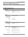
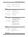
Appendix F: RMC100 Specifications .......................................... F-1
Hardware specifications of the RMC.
Appendix G: Glossary ................................................................. G-1
Concise explanations of words specific to the field of motion control.
Appendix H: ASCII Table ............................................................. H-1
Table of the 128 standard ASCII characters.
Index ...................................................................................... Index-1
iii
RMC100 and RMCWin User Manual
iv
RMC100 and RMCWin User Manual
Contents
Table of Contents
DISCLAIMER ......................................................................................................... XXI
INTRODUCING THE RMC100 SERIES ..................................................................... 1-1
RMC100 Overview ................................................................................................... 1-1
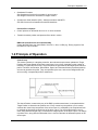
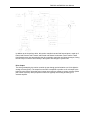
Principle of Operation ............................................................................................ 1-3
STARTING UP THE RMC....................................................................................... 2-0
Step-by-Step RMC Startup ..................................................................................... 2-0
Setup Details ........................................................................................................... 2-4
Scaling Overview ................................................................................................................... 2-4
Advanced Scaling .................................................................................................................. 2-5
Tuning .................................................................................................................................... 2-5
Tuning Overview ................................................................................................................ 2-5
Tuning a Position Axis ........................................................................................................ 2-7
Tuning a Torque Motor ....................................................................................................... 2-9
Tuning a Position-Pressure System ................................................................................. 2-12
Tuning Wizard: Overview ................................................................................................. 2-15
Tuning Wizard: Obtaining Plots........................................................................................ 2-16
Open Loop Moves ........................................................................................................ 2-17
Closed Loop Moves ...................................................................................................... 2-17
USING RMCWIN ................................................................................................. 3-0
RMCWin Overview .................................................................................................. 3-0
Screen Layout ......................................................................................................... 3-1
Understanding the Screen ..................................................................................................... 3-1
Command Area ...................................................................................................................... 3-2
Parameter Area...................................................................................................................... 3-3
Plot Time Area ....................................................................................................................... 3-4
Status Area ............................................................................................................................ 3-4
Status Bar .............................................................................................................................. 3-5
Toolbar ................................................................................................................................... 3-5
Connecting to an RMC ........................................................................................... 3-6
Connecting RMCWin to an RMC ........................................................................................... 3-6
Setting the Firewall to Allow RMC100 Ethernet Browsing ..................................................... 3-8
Using the Communication Options Tab ................................................................................. 3-9
Working Offline .................................................................................................................... 3-10
Configuration Conflict Detection .......................................................................................... 3-12
Resolve Configuration Conflict Dialog Box .......................................................................... 3-12
Communication Drivers ....................................................................................................... 3-13
Communication Driver: Serial Overview .......................................................................... 3-13
Communication Driver: Serial Configuration .................................................................... 3-14
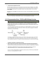
Communication Driver: TCP/IP Direct to RMC-ENET Overview ..................................... 3-16
Communication Driver: TCP/IP Direct to RMC-ENET Configuration ............................... 3-17
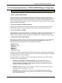
Communication Driver: TCP/IP-to-RS232 Bridge Overview ............................................ 3-19
Communication Driver: TCP/IP-to-RS232 Bridge Configuration ..................................... 3-20
v
RMC100 and RMCWin User Manual
Basic Topics ......................................................................................................... 3-21
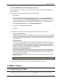
Selecting Your View ............................................................................................................. 3-21
Accessing Context Sensitive Help ....................................................................................... 3-23
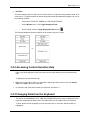
Changing Data from the Keyboard ...................................................................................... 3-23
Read-back versus Write Mode ............................................................................................ 3-24
RMC Configuration Dialog Box ............................................................................................ 3-25
RMC100/101 CPU Options Dialog Box ............................................................................... 3-26
Using Pop-up Editors ........................................................................................................... 3-26
Using the Status Bits Window.............................................................................................. 3-27
Using the Command Log ..................................................................................................... 3-27
Using the Parameter Error List Window .............................................................................. 3-29
Using the I/O Bit Monitor ...................................................................................................... 3-30
Using Stored Commands ..................................................................................................... 3-30
Changing the Axis Names ................................................................................................... 3-31
Using Multiple RMCs ........................................................................................................... 3-32
File Types ............................................................................................................................ 3-32
Creating a New Board File ................................................................................................... 3-33
Changing Between Board Files ........................................................................................... 3-34
Editing Board File Information ............................................................................................. 3-35
Load Parameters Command................................................................................................ 3-35
Scale/Offset Calibration Utilities .......................................................................................... 3-36
Using the Scale/Offset Calibration Utilities ...................................................................... 3-36
Position Scale/Offset Calibration Utility ............................................................................ 3-36
MDT Scale/Offset Calibration Utility ................................................................................. 3-37
SSI Scale/Offset Calibration Utility ................................................................................... 3-38
Quadrature Calibration Utility ........................................................................................... 3-38
Resolver Scale/Offset Calibration Utility .......................................................................... 3-39
Pressure Scale/Offset Calibration Utility .......................................................................... 3-40
Differential Force Scale/Offset Calibration Utility ............................................................. 3-40
Using Plots ............................................................................................................ 3-43
Using Graphs of Axis Moves ............................................................................................... 3-43
Opening a Plot Window ....................................................................................................... 3-44
Reading Plot Data from the Motion Controller ..................................................................... 3-44
Selecting the Data to Plot .................................................................................................... 3-44
Using the Plot Detail Window .............................................................................................. 3-45
Viewing the Raw Plot Data .................................................................................................. 3-46
Saving and Restoring Plots ................................................................................................. 3-47
Printing a Plot....................................................................................................................... 3-47
Plot Time .............................................................................................................................. 3-48
Special Status Values Available In Plots ............................................................................. 3-48
Target Speed.................................................................................................................... 3-48
Raw Transducer Counts .................................................................................................. 3-49
Sum of Errors Squared .................................................................................................... 3-49
Sum of Analog Errors Squared ........................................................................................ 3-49
Table Editors ......................................................................................................... 3-49
Table Editor Basics .............................................................................................................. 3-49
Editing the Input to Event Table........................................................................................... 3-51
Editing the Stored Command Table..................................................................................... 3-53
Editing the Profile Table ....................................................................................................... 3-53
Step Table Editor .................................................................................................. 3-53
Step Table Editor: Overview ................................................................................................ 3-53
Step Table Editor: Keyboard Shortcuts ............................................................................... 3-56
LCD Screen Editor ................................................................................................ 3-58
vi
RMC100 and RMCWin User Manual
LCD Screen Editor: Overview .............................................................................................. 3-58
Editor Window Elements ...................................................................................................... 3-59
LCD Screen Editor: Editor Window Elements .................................................................. 3-59
LCD Screen Editor: Tree Pane Details ............................................................................ 3-60
LCD Screen Editor: Screen Pane Details ........................................................................ 3-60
LCD Screen Editor: Field Pane Details ............................................................................ 3-61
LCD Screen Editor: Data Tab Details .............................................................................. 3-61
LCD Screen Editor: Format Tab Details .......................................................................... 3-63
LCD Screen Editor: Toolbar Details ................................................................................. 3-65
LCD Screen Editor: Status Bar Details ............................................................................ 3-66
Using the LCD Screen Editor ............................................................................................... 3-66
LCD Screen Editor: Using LCD Screen Files ................................................................... 3-66
LCD Screen Editor: Uploading and Downloading LCD Screens ..................................... 3-67
LCD Screen Editor: Using the Clipboard ......................................................................... 3-68
LCD Screen Editor: Changing the View Options ............................................................. 3-69
LCD Screen Editor: Keyboard Shortcuts ......................................................................... 3-70
Using Screens ...................................................................................................................... 3-71
LCD Screen Editor: Adding and Removing Screens ....................................................... 3-71
LCD Screen Editor: Changing the Screen Order ............................................................. 3-72
LCD Screen Editor: Editing Screen Text .......................................................................... 3-72
LCD Screen Editor: Selecting Insert or Overtype Mode .................................................. 3-73
LCD Screen Editor: Renaming Screens .......................................................................... 3-74
Using Fields ......................................................................................................................... 3-74
LCD Screen Editor: Adding and Removing Fields ........................................................... 3-74
LCD Screen Editor: Moving and Resizing Fields ............................................................. 3-75
LCD Screen Editor: Editing Field Properties .................................................................... 3-76
LCD Screen Editor: Using Editable Fields ....................................................................... 3-77
LCD Screen Editor: Using Fields with Multiple Write Locations ...................................... 3-77
LCD Screen Editor: Renaming Fields .............................................................................. 3-79
Curve Tool ............................................................................................................. 3-80
Curve Tool: Overview .......................................................................................................... 3-80
Screen Elements.................................................................................................................. 3-82
Curve Tool: Screen Elements .......................................................................................... 3-82
Curve Tool: Graph View ................................................................................................... 3-83
Curve Tool: Detail Window............................................................................................... 3-84
Curve Tool: Spreadsheet View ........................................................................................ 3-85
Curve Tool: Toolbar ......................................................................................................... 3-86
Curve Tool: Status Bar ..................................................................................................... 3-87
Using the Curve Tool ........................................................................................................... 3-88
Curve Tool: Units of Measurement .................................................................................. 3-88
Curve Tool: Using Curve Files ......................................................................................... 3-90
Curve Tool: Mouse Commands ....................................................................................... 3-90
Curve Tool: Keyboard Shortcuts ...................................................................................... 3-92
Using the Graph View .......................................................................................................... 3-93
Curve Tool: Graph View Options ..................................................................................... 3-93
Curve Tool: Showing Velocity and Acceleration .............................................................. 3-94
Curve Tool: Using the Grid............................................................................................... 3-95
Curve Tool: Adjusting the Scales ..................................................................................... 3-96
Curve Tool: Using the Scale Bars .................................................................................... 3-97
Curve Tool: Changing the Orientation ............................................................................. 3-98
Curve Tool: Scrolling ........................................................................................................ 3-98
Curve Tool: Zooming In and Out ...................................................................................... 3-99
Using the Spreadsheet View ............................................................................................. 3-100
Curve Tool: Spreadsheet View Options ......................................................................... 3-100
Curve Tool: Selecting Cells ............................................................................................ 3-100
vii
RMC100 and RMCWin User Manual
Curve Tool: Editing Cells ................................................................................................ 3-101
Curve Tool: Deleting Cells ............................................................................................. 3-102
Curve Tool: Cutting and Copying Cells .......................................................................... 3-103
Curve Tool: Pasting Cells ............................................................................................... 3-104
Curve Tool: The Insertion Point ..................................................................................... 3-104
Curve Tool: Resizing columns ....................................................................................... 3-105
Using Curves ..................................................................................................................... 3-105
Curve Tool: Selecting Which Curves to Display ............................................................ 3-105
Curve Tool: Selecting the Active Axis ............................................................................ 3-106
Curve Tool: Copying Curves between Axes .................................................................. 3-107
Curve Tool: Importing and Exporting Curves ................................................................. 3-108
Curve Tool: Uploading and Downloading Curves .......................................................... 3-109
Curve Tool: Converting a Plot to a Curve ...................................................................... 3-110
Curve Tool: Erasing a Curve .......................................................................................... 3-112
Curve Tool: Curve Properties and Editing Options ........................................................ 3-113
Curve Tool: Curve Axis Labels....................................................................................... 3-114
Curve Tool: Curve Limits ................................................................................................ 3-114
Curve Tool: Standard vs. Enhanced Curves .................................................................. 3-115
Curve Tool: Auto Repeat Curves ................................................................................... 3-117
Curve Tool: Enforcing Limits .......................................................................................... 3-118
Curve Tool: Linking Curves ............................................................................................ 3-118
Using Points ....................................................................................................................... 3-119
Curve Tool: Selecting Points .......................................................................................... 3-119
Curve Tool: Determining a Point's Exact Location ......................................................... 3-121
Curve Tool: Adding Points ............................................................................................. 3-122
Curve Tool: Deleting Points ........................................................................................... 3-122
Curve Tool: Point Properties .......................................................................................... 3-123
Curve Tool: Moving Points ............................................................................................. 3-124
Curve Tool: Selecting Linear or Cubic Segments .......................................................... 3-125
Curve Tool: Changing a Point's Velocity ........................................................................ 3-126
Curve Tool: Expanding or Contracting Points ................................................................ 3-126
Address Tool ....................................................................................................... 3-127
Address Tool: Overview ..................................................................................................... 3-127
Address Tool: Bookmarking Addresses............................................................................. 3-128
Address Tool: Using with the Event Step Editor ................................................................ 3-129
Address Tool: Keeping the Address Tool in the Foreground ............................................ 3-129
Advanced Topics ................................................................................................ 3-130
Downloading New RMC100 Firmware............................................................................... 3-130
Downloading New Serial/Ethernet Firmware ..................................................................... 3-131
Options: Preferences ......................................................................................................... 3-131
Forcing Initialization ........................................................................................................... 3-132
Using Look-only Mode ....................................................................................................... 3-133
Using PC Mode .................................................................................................................. 3-133
Command-Line Options ..................................................................................................... 3-133
CONTROLLER FEATURES ..................................................................................... 4-0
Event Control Overview ......................................................................................... 4-0
Flash Memory.......................................................................................................... 4-2
Gearing Axes .......................................................................................................... 4-3
LED Indicators ........................................................................................................ 4-7
Reference Axis Filtering ....................................................................................... 4-10
viii
RMC100 and RMCWin User Manual
Speed Control ....................................................................................................... 4-15
Rotational Mode .................................................................................................... 4-17
Spline Overview .................................................................................................... 4-18
Synchronizing Axes.............................................................................................. 4-26
Teach Mode Overview .......................................................................................... 4-27
VC2100 and VC2124 Voltage-to-Current Converters .......................................... 4-28
Position/Pressure Control .................................................................................... 4-30
Position-Pressure Overview ................................................................................................ 4-30
Position-Pressure Setup ...................................................................................................... 4-32
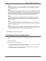
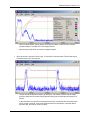
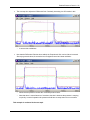
Position-Pressure Example (Part 1) .................................................................................... 4-37
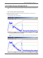
Position-Pressure Example (Part 2) .................................................................................... 4-45
Position-Pressure Example (Part 3) .................................................................................... 4-51
Position-Pressure Example (Part 4) .................................................................................... 4-52
Position-Pressure Example (Part 5) .................................................................................... 4-56
COMMUNICATIONS ............................................................................................... 5-0
Digital I/O ................................................................................................................. 5-0
Digital I/O Specifications ........................................................................................................ 5-0
Digital I/O Wiring .................................................................................................................... 5-1
CPU Digital Outputs ........................................................................................................... 5-1
DI/O Digital Outputs ........................................................................................................... 5-1
CPU Inputs ......................................................................................................................... 5-3
DI/O Inputs ......................................................................................................................... 5-3
Using Counters ...................................................................................................................... 5-6
CPU Digital I/O....................................................................................................................... 5-7
Using the CPU Digital I/O ................................................................................................... 5-7
Sensor Digital I/O ................................................................................................................... 5-8
Using the Sensor Digital I/O ............................................................................................... 5-8
Communication Digital I/O ..................................................................................................... 5-9
Using the Communication Digital I/O ................................................................................. 5-9
Features Shared by All Modes ......................................................................................... 5-11
Using Command Mode .................................................................................................... 5-13
Using Input to Event Mode ............................................................................................... 5-15
Using Parallel Position Mode ........................................................................................... 5-18
Using Parallel Event Mode ............................................................................................... 5-22
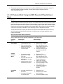
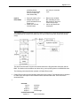
Technical Brief: Using the RMC Discrete I/O Command Mode ....................................... 5-24
Technical Brief: Using the RMC Discrete I/O Input to Event Mode ................................. 5-28
Technical Brief: Using the RMC Discrete I/O Parallel Position Mode .............................. 5-35
Technical Brief: Using the RMC Discrete I/O Parallel Event Mode ................................. 5-42
Ethernet ................................................................................................................. 5-48
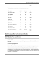
RMC Ethernet Module Overview ......................................................................................... 5-48
Using the RMC ENET with Programmable Controllers ....................................................... 5-49
Using the RMC ENET with RMCWin ................................................................................... 5-51
Ethernet Setup Topics ......................................................................................................... 5-51
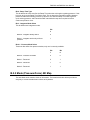
RMC Ethernet IP Address Setup ..................................................................................... 5-51
Setting up a Stand-alone TCP/IP Control Network .......................................................... 5-54
RMC Ethernet Firmware Screen ...................................................................................... 5-55
RMC Ethernet Statistics ................................................................................................... 5-56
RMC Ethernet Activity Log ............................................................................................... 5-59
Ethernet Informational Topics .............................................................................................. 5-60
Understanding IP Addressing .......................................................................................... 5-60
ix
RMC100 and RMCWin User Manual
RMC Ethernet Protocols .................................................................................................. 5-61
Controlling and Monitoring the RMC over Ethernet ............................................................. 5-65
Allen-Bradley Controllers ................................................................................................. 5-65
Using Allen-Bradley Controllers with the RMC Ethernet Module ................................. 5-65
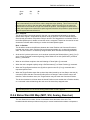
RMC Register Map (Allen-Bradley) .............................................................................. 5-69
Using EtherNet/IP with the ControlLogix ...................................................................... 5-80
Automationdirect.com's DL205/305 ................................................................................. 5-80
Using Automationdirect.com PLCs with the RMC ENET ............................................. 5-80
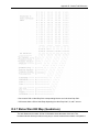
RMC Register Map (Automationdirect.com)................................................................. 5-84
EtherNet/IP Controllers .................................................................................................... 5-94
Using EtherNet/IP with the RMC ENET ....................................................................... 5-94
Configuring an RMC EtherNet/IP I/O Connection for the ControlLogix ....................... 5-95
Establishing Multiple I/O Connections with a Single RMC ......................................... 5-100
Controlling the RMC over EtherNet/IP I/O .................................................................. 5-100
Handling Broken I/O Connections .............................................................................. 5-103
RMC EtherNet/IP Definition ........................................................................................ 5-106
RMC EtherNet/IP Object Model .............................................................................. 5-106
EtherNet/IP Performance ........................................................................................... 5-108
EtherNet/IP Performance Overview ........................................................................ 5-108
Evaluating the Load on the RMC ENET ................................................................. 5-108
Evaluating the Load on the 1756-ENET ................................................................. 5-109
Evaluating the Load on the 1756-ENBT ................................................................. 5-111
Predicting the Effect of Collisions ........................................................................... 5-111
Setting Up Large EtherNet/IP Networks ................................................................. 5-118
Modicon Quantum .......................................................................................................... 5-120
Using Modicon PLCs with the RMC Ethernet Module ................................................ 5-120
RMC Register Map (Modbus/TCP and Modbus/RTU) ............................................... 5-121
Omron CS1 and CV PLCs ............................................................................................. 5-130
Using Omron PLCs with the RMC ENET ................................................................... 5-130
RMC Register Map (Omron FINS) ............................................................................. 5-136
Rockwell Software RSView32 ........................................................................................ 5-145
Using Rockwell Software's RSView32 with the RMC Ethernet Module ..................... 5-145
RMC Register Map (Allen-Bradley) ............................................................................ 5-147
Siemens Simatic TI505 .................................................................................................. 5-158
Using the Siemens Simatic TI505 with the RMC Ethernet Module ............................ 5-158
RMC Register Map (Siemens TI505) ......................................................................... 5-158
Siemens S7 .................................................................................................................... 5-167
RMC Register Map (Siemens S7) .............................................................................. 5-167
SoftPLC's SoftPLC ......................................................................................................... 5-175
Using the SoftPLC with the RMC Ethernet Module .................................................... 5-175
RMC Register Map (SoftPLC) .................................................................................... 5-176
Other PLCs and PC-based Control Packages ............................................................... 5-177
Using Other Ethernet Packages with the RMC ENET ............................................... 5-177
Custom Ethernet Devices and Applications ................................................................... 5-177
Using the RMCLink ActiveX Control and .Net Assembly Component ....................... 5-177
Using Sockets to Access the RMC ENET .................................................................. 5-177
Modbus Plus ....................................................................................................... 5-179
Using the Modicon Modbus Plus Communication Module ................................................ 5-179
Changing the Modbus Plus Node Address ........................................................................ 5-180
Reading and Writing Modbus Plus Registers .................................................................... 5-180
RMC Register Map (Modbus Plus) .................................................................................... 5-181
Using the TSX Premium and Modbus Plus ....................................................................... 5-190
Modbus Plus Global Data .................................................................................................. 5-192
Using Modbus Plus Global Data .................................................................................... 5-192
Using Modicon’s Peer Cop to Read Global Data ........................................................... 5-192
x
RMC100 and RMCWin User Manual
MSTR Modicon Ladder Logic Block .................................................................................. 5-195
Using the MSTR Modicon Ladder Logic Block .............................................................. 5-195
MSTR Block Read Operation ......................................................................................... 5-197
MSTR Block Write Operation ......................................................................................... 5-200
MSTR Block Read Global Data Operation ..................................................................... 5-203
MSTR Block Peer Cop Health Operation ....................................................................... 5-204
MSTR Block Error Codes ............................................................................................... 5-206
PROFIBUS-DP ..................................................................................................... 5-208
PROFIBUS-DP .................................................................................................................. 5-208
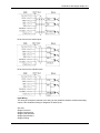
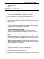
PROFIBUS Configuration .................................................................................................. 5-209
Configuring a PROFIBUS-DP Network with COM PROFIBUS ......................................... 5-212
Configuring a PROFIBUS-DP Network with SST Profibus Configuration ......................... 5-214
Configuring a PROFIBUS-DP Network with SyCon .......................................................... 5-215
Compact Mode................................................................................................................... 5-217
Using the PROFIBUS-DP Compact Mode ..................................................................... 5-217
Compact Mode Input Register Overview ....................................................................... 5-218
Compact Mode Output Register Overview .................................................................... 5-221
Message Mode .................................................................................................................. 5-223
Using the PROFIBUS-DP Message Mode ..................................................................... 5-223
RMC Register Map (PROFIBUS-DP Message Mode) ................................................... 5-225
Serial (RS-232/422/485)....................................................................................... 5-235
RMC SERIAL Overview ..................................................................................................... 5-235
Configuration and Wiring ................................................................................................... 5-236
Configuring the RMC SERIAL ........................................................................................ 5-236
RMC SERIAL Firmware Screen ..................................................................................... 5-237
Line Drivers: RS-232/422/485 ........................................................................................ 5-238
Serial Network Topologies ............................................................................................. 5-239
RS-232 Wiring for the RMC SERIAL ............................................................................. 5-243
RS-422/485 Wiring for the RMC SERIAL ...................................................................... 5-244
RS-422/485 Termination and Biasing ............................................................................ 5-246
RMC SERIAL Protocols ..................................................................................................... 5-250
Using Modbus/RTU with the RMC SERIAL ................................................................... 5-250
Using DF1 (Full- and Half-Duplex) with the RMC SERIAL ............................................ 5-251
Using the Mitsubishi No Protocol with the RMC SERIAL .............................................. 5-256
Using the Mitsubishi Bidirectional Protocol with the RMC SERIAL ............................... 5-261
RMC CPU RS232 Port ......................................................................................... 5-265
Using the CPU RS-232 Port with RMCWin ....................................................................... 5-265
RMCLink ActiveX Control and .NET Assembly ................................................................. 5-265
RS232 Wiring ..................................................................................................................... 5-267
LCD420 Terminal ................................................................................................ 5-270
LCD Display Terminal Overview ........................................................................................ 5-270
Using the LCD420 Terminal .............................................................................................. 5-271
Programming the LCD420 Terminal .................................................................................. 5-274
Status Map .......................................................................................................... 5-275
Using the Status Map Editor .............................................................................................. 5-275
Default Status Map Data .................................................................................................... 5-277
Communication Tasks........................................................................................ 5-278
Reading Plots from the Communication Module ............................................................... 5-278
Downloading Splines to the RMC ...................................................................................... 5-280
Parameter Error Values ..................................................................................................... 5-291
TRANSDUCER INTERFACE MODULES ..................................................................... 6-0
xi
RMC100 and RMCWin User Manual
Analog ..................................................................................................................... 6-0
Analog Transducer Overview ................................................................................................ 6-0
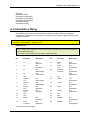
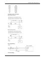
Analog Transducer Wiring ..................................................................................................... 6-1
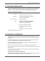
Analog Transducer Configuration .......................................................................................... 6-3
Analog Transducer LED Indicators ........................................................................................ 6-6
Analog Transducer Specifications ......................................................................................... 6-6
Analog Transducer Scaling .................................................................................................... 6-8
Setup Details ........................................................................................................................ 6-10
Using Analog Channels as Position Inputs ...................................................................... 6-10
Using Analog Channels as Velocity Inputs ...................................................................... 6-12
Using Analog Channels as Pressure Inputs .................................................................... 6-14
Using Analog Channels as Differential Force Inputs ....................................................... 6-15
Usage Details ....................................................................................................................... 6-16
Using Position and Velocity Joysticks .............................................................................. 6-16
Using an External Target Generator ................................................................................ 6-17
Controlling Speed from a Tachometer Feedback ............................................................ 6-18
Controlling Analog Position, Pressure, or Force .............................................................. 6-19
MDT........................................................................................................................ 6-20
MDT Overview ..................................................................................................................... 6-20
MDT Wiring .......................................................................................................................... 6-21
MDT Configuration ............................................................................................................... 6-24
MDT LED Indicators............................................................................................................. 6-25
MDT Specifications .............................................................................................................. 6-26
MDT Scaling ........................................................................................................................ 6-27
Quadrature with Analog Output ........................................................................... 6-31
Quadrature with Analog Output Overview ........................................................................... 6-31
Quadrature Wiring................................................................................................................ 6-33
Quadrature/Analog Cable .................................................................................................... 6-37
Quadrature Configuration .................................................................................................... 6-37
Quadrature LED Indicators .................................................................................................. 6-38
Quadrature Specifications ................................................................................................... 6-39
Quadrature Scaling .............................................................................................................. 6-41
Homing a Quadrature Axis .................................................................................................. 6-44
Quadrature with Stepper Output.......................................................................... 6-45
Quadrature with Stepper Output Overview .......................................................................... 6-45
Stepper Wiring ..................................................................................................................... 6-48
Stepper Configuration .......................................................................................................... 6-50
Stepper LED Indicators ........................................................................................................ 6-51
Stepper Specifications ......................................................................................................... 6-52
Stepper Scaling.................................................................................................................... 6-53
Stepper Compensation ........................................................................................................ 6-58
Resolver ................................................................................................................ 6-59
Resolver Overview ............................................................................................................... 6-59
Resolver Wiring.................................................................................................................... 6-61
Resolver Configuration ........................................................................................................ 6-63
Resolver LED Indicators ...................................................................................................... 6-64
Resolver Specifications ....................................................................................................... 6-64
Resolver Scaling .................................................................................................................. 6-66
SSI.......................................................................................................................... 6-67
SSI Overview ....................................................................................................................... 6-67
SSI Wiring ............................................................................................................................ 6-68
SSI Configuration ................................................................................................................. 6-70
SSI LED Indicators............................................................................................................... 6-74
xii
RMC100 and RMCWin User Manual
SSI Specifications ................................................................................................................ 6-75
SSI Scaling .......................................................................................................................... 6-76
SUPPORT AND TROUBLESHOOTING ....................................................................... 7-0
Warranty .................................................................................................................. 7-0
Troubleshooting ..................................................................................................... 7-0
Programming Hints ................................................................................................................ 7-0
Error Handling ........................................................................................................................ 7-1
RMC Module Problems .......................................................................................................... 7-1
Hydraulic System Problems ................................................................................................... 7-2
Technical Support .................................................................................................. 7-6
Technical Support .................................................................................................................. 7-6
Parameter Errors .................................................................................................... 7-7
A valid segment has not been calculated .............................................................................. 7-7
Acceleration overflow while calculating spline ....................................................................... 7-7
Attempt to enter pressure immediately failed ........................................................................ 7-7
Attempt to go beyond extend limit ......................................................................................... 7-8
Attempt to go beyond retract limit .......................................................................................... 7-8
Attempt to send spline through Spline Download Area while download in progress ............ 7-8
Attempt to write to the Spline Download Area of a non-existent or non-spline capable axis 7-8
Auto-Repeat Should Not be Used on Linear Axes with a Curve that Does Not Match Endpoints ..... 7-9
Axis must be initialized to use this command ........................................................................ 7-9
Axis must be stopped for this command ................................................................................ 7-9
Both sync bits cannot be set in the "Mode" word .................................................................. 7-9
Cannot clear a segment while interpolating ........................................................................... 7-9
Cannot home an axis while synchronized ........................................................................... 7-10
Cannot issue a ’r;Z’ or ’r;z’ command to a synchronized axis ............................................. 7-10
Cannot overflow command pressure ................................................................................... 7-10
Cannot use synchronization with speed control .................................................................. 7-10
Command pressure cannot be less than pressure set A..................................................... 7-10
Command pressure cannot be less than pressure set B..................................................... 7-11
Dead band eliminator out of range ...................................................................................... 7-11
Drive transfer percentage out of range ................................................................................ 7-11
"Event Step Edit" indices are invalid .................................................................................... 7-11
Extend limit must be greater than retract limit ..................................................................... 7-11
Feed forward terms must have the same sign .................................................................... 7-11
Fewer segments than were requested to be cleared existed .............................................. 7-12
Flash contained no data on startup ..................................................................................... 7-12
Function in the Function (,) Command Out of Range .......................................................... 7-12
Gear ratio denominator is zero ............................................................................................ 7-13
Gearing and Synchronization Illegal in Open Loop ............................................................. 7-13
Incompatible sync mode words ........................................................................................... 7-13
Internal error while using the Spline Download Area........................................................... 7-13
Invalid Address Used in Add (+) or Subtract (-) Command ................................................. 7-13
Invalid command received ................................................................................................... 7-13
Invalid command value ........................................................................................................ 7-14
Invalid Gear Master Selected .............................................................................................. 7-14
Invalid Interval Table Format in the Spline Download Area ................................................ 7-15
Invalid MODE bits set for this command.............................................................................. 7-15
Invalid Point Count in the Spline Download Area ................................................................ 7-15
Invalid scale value................................................................................................................ 7-15
Invalid Screen Number in the Display LCD Screen ($) Command...................................... 7-16
Invalid step number given in "Start Events" command ........................................................ 7-16
Maximum Steps per Millisecond parameter out of range .................................................... 7-16
xiii
RMC100 and RMCWin User Manual
Move would cause discontinuity .......................................................................................... 7-16
No Axes Selected for Use by the Function (,) Command .................................................... 7-16
No initialized pressure axis is assigned ............................................................................... 7-17
Non-existent pressure axis selected in "Config" word ......................................................... 7-17
Numeric overflow while sending a spline to the Spline Download Area .............................. 7-17
One or more synced axes are uninitialized ......................................................................... 7-18
Overflow while adding point. Point not added ..................................................................... 7-18
Point cannot be added during calculations .......................................................................... 7-18
Position overflow while interpolating spline ......................................................................... 7-18
Pressure Control went outside position limits ...................................................................... 7-18
Pressure set A cannot be less than pressure set B............................................................. 7-18
Reached command position while regulating pressure ....................................................... 7-19
Requested drive too large .................................................................................................... 7-19
Reserved command parameter must be 0 .......................................................................... 7-19
Reserved parameters must be zero .................................................................................... 7-19
Resetting the position is not allowed in this state ................................................................ 7-19
Resetting the position would cause a position overflow ...................................................... 7-20
Spline Points downloaded out-of-order................................................................................ 7-20
SSI transducer overflow ....................................................................................................... 7-20
SSI transducer noise ........................................................................................................... 7-20
Step Number in Teach (t) or Function (,) Command Out of Range ..................................... 7-21
Steps per Rev and Position Units per Rev must not be zero .............................................. 7-21
Storage of parameters to Flash failed.................................................................................. 7-21
Storage of splines to Flash failed......................................................................................... 7-21
Superimposed and gear mode bits required by Master Relative Sine Move command. .... 7-21
Synchronized axis was incorrectly dropped ........................................................................ 7-21
Target position moved outside limits ................................................................................... 7-22
Target position must be equal to the first spline point ......................................................... 7-22
The Accel Field Must Be Zero in the Command Issued ...................................................... 7-23
The acceleration or deceleration ramp is too slow .............................................................. 7-23
The axis must be stopped before following a spline ............................................................ 7-23
The command acceleration is invalid................................................................................... 7-23
The command deceleration is invalid .................................................................................. 7-24
The spline interval cannot be set below 5 ........................................................................... 7-24
Invalid command for this transducer type ............................................................................ 7-24
There must be at least two points to begin calculations ...................................................... 7-24
Requested sine-move speed too low .................................................................................. 7-25
Too many points attempted in the Spline Download Area .................................................. 7-25
Too many spline points. Point not added ............................................................................ 7-26
Too many superimposed moves attempted ........................................................................ 7-26
Unable to Download a Curve over an Auto-Repeat Curve Using Spline Download Area... 7-26
Unable to Download Curve over an Auto-Repeat Curve ..................................................... 7-26
Velocity overflow while interpolating spline ......................................................................... 7-26
Unknown Parameter Error ................................................................................................... 7-27
APPENDIX A: COMMAND REFERENCE ................................................................... A-1
General ASCII Commands..................................................................................... A-1
I-PD Position Move Command ............................................................................................. A-1
Set Count Offset Command .................................................................................................. A-2
Display LCD Screen Command ............................................................................................ A-3
MulDiv Command ................................................................................................................. A-3
Add Command ...................................................................................................................... A-6
Function Command............................................................................................................... A-7
Subtract Command ............................................................................................................... A-9
Poll Command .................................................................................................................... A-10
Arm Home Command ......................................................................................................... A-14
xiv
RMC100 and RMCWin User Manual
Change Acceleration Command ......................................................................................... A-14
Amp Enable/Disable Command.......................................................................................... A-14
Clear Spline Segments Command ..................................................................................... A-15
Set Position/Pressure Command........................................................................................ A-16
Change Deceleration Command ........................................................................................ A-16
Start Events Command ....................................................................................................... A-17
Set Feed Forward Command ............................................................................................. A-17
Follow Spline Segment Command ..................................................................................... A-17
Go Command...................................................................................................................... A-19
Halt Command .................................................................................................................... A-20
Set Integral Drive Command .............................................................................................. A-20
Set Integral Drive to Null Drive Command .......................................................................... A-21
Relative Move Command ................................................................................................... A-21
Disable Drive Output Command ......................................................................................... A-21
Limit Drive Command ......................................................................................................... A-21
Set Extended Link Value Command ................................................................................... A-22
Set Mode Command ........................................................................................................... A-22
Set Null Drive Command .................................................................................................... A-23
Set Null Drive to Integral Drive Command .......................................................................... A-23
Open Loop Command ........................................................................................................ A-23
Set Parameters Command ................................................................................................. A-25
Quit Events Command ........................................................................................................ A-25
Reset Position Command ................................................................................................... A-26
Restore Null Drive Command ............................................................................................. A-26
Restore Integral Drive Command ....................................................................................... A-26
Save Null Drive Command ................................................................................................. A-27
Save Integral Drive Command ............................................................................................ A-27
Set Spline Interval/End Segment Command ...................................................................... A-27
Set Spline Interval/End Segment Command ...................................................................... A-28
Teach Step Command ........................................................................................................ A-29
Update Flash Command ..................................................................................................... A-29
Update Flash Segment Command ..................................................................................... A-30
Set Speed (Unsigned) Command ....................................................................................... A-30
Set Speed (Signed) Command ........................................................................................... A-30
Reference Command .......................................................................................................... A-31
Spline Relative Sine Move .................................................................................................. A-32
New Spline Point Command ............................................................................................... A-34
Start a Graph Command ..................................................................................................... A-34
Zero Position/Set Target Command ................................................................................... A-34
Offset Positions Command ................................................................................................. A-35
Reset Outputs Command ................................................................................................... A-35
Set Outputs Command ....................................................................................................... A-36
Simulate Rising Edge Command ........................................................................................ A-37
Simulate Falling Edge Command ....................................................................................... A-38
Sine Move Command ......................................................................................................... A-38
Set and Reset Wait Bits Command .................................................................................... A-40
Sine Move Continuous Command ...................................................................................... A-41
Follow Spline Relative Command ....................................................................................... A-42
Map Output to Axis Position ............................................................................................... A-43
Move Relative to An Axis .................................................................................................... A-44
Set Parameter On-the-Fly................................................................................................... A-46
Pressure/Force Control ASCII Commands ........................................................ A-47
Set Bias Drive Command ................................................................................................... A-47
Start Events Command ....................................................................................................... A-48
Set Mode Command ........................................................................................................... A-48
xv
RMC100 and RMCWin User Manual
Open Loop Command ........................................................................................................ A-49
Set Parameters Command ................................................................................................. A-50
Quit Events Command ........................................................................................................ A-51
Set Pressure Ramp Time Command .................................................................................. A-51
Set Pressure Command ..................................................................................................... A-52
Set Pressure Set A Command ............................................................................................ A-52
Set Pressure Set B Command ............................................................................................ A-53
Set Parameter On-the-Fly................................................................................................... A-53
Programmable Controller Commands................................................................ A-54
Command Words for Digital I/O’s Command Mode ........................................................... A-54
Command Words for PROFIBUS-DP Compact Mode ....................................................... A-58
Receiving Data from the Motion Controller ......................................................................... A-61
Sending Data from the PLC ................................................................................................ A-61
Open Loop Using Profile Commands ................................................................................. A-61
Set Parameter Commands ................................................................................................. A-63
Set Profile Commands ........................................................................................................ A-65
ASCII Commands ............................................................................................................... A-70
Go/Set Pressure Using Profile Commands ........................................................................ A-70
Get Parameter Commands ................................................................................................. A-72
Get Profile Commands ....................................................................................................... A-74
Set Parameter On-the-fly PLC Commands ........................................................................ A-80
Event Step Edit Commands ................................................................................................ A-82
Command/Commanded Axes ............................................................................................. A-86
LINK TYPE/NEXT ............................................................................................................... A-86
Diagnostics Command ........................................................................................................ A-87
Download Graph Data Commands ..................................................................................... A-88
Event Step Transfer Command .......................................................................................... A-93
APPENDIX B: COMMAND FIELD REFERENCE .......................................................... B-1
Position Command Fields ..................................................................................... B-1
MODE (Non-Pressure/Force) ............................................................................................... B-1
Mode (Non-Pressure/Force) Bit Map .................................................................................... B-6
Acceleration .......................................................................................................................... B-6
Deceleration .......................................................................................................................... B-8
Speed .................................................................................................................................... B-8
Command Value ................................................................................................................... B-8
COMMAND ......................................................................................................................... B-10
Pressure/Force Command Fields ....................................................................... B-13
Mode (Pressure/Force) ....................................................................................................... B-13
Mode (Pressure/Force) Bit Map .......................................................................................... B-14
Pressure Set A .................................................................................................................... B-15
Pressure Set B .................................................................................................................... B-16
Ramp Time (Pressure/Force) ............................................................................................. B-16
Command Value ................................................................................................................. B-17
COMMAND ......................................................................................................................... B-19
APPENDIX C: PARAMETER FIELD REFERENCE ....................................................... C-1
MDT, SSI, Analog, Resolver Position Parameters ............................................... C-1
Configuration Word ............................................................................................................... C-1
Configuration Word Bit Map .................................................................................................. C-4
Configuration Bits - MDT Specific ......................................................................................... C-5
Configuration Bits - SSI Specific ........................................................................................... C-6
Configuration Bits - Analog Specific ..................................................................................... C-6
Configuration Bits - Resolver Specific .................................................................................. C-7
xvi
RMC100 and RMCWin User Manual
Scale ..................................................................................................................................... C-7
Offset .................................................................................................................................... C-8
Extend Limit .......................................................................................................................... C-8
Retract Limit .......................................................................................................................... C-9
Proportional Gain .................................................................................................................. C-9
Integral Gain ....................................................................................................................... C-10
Differential Gain .................................................................................................................. C-10
Extend Feed Forward ......................................................................................................... C-11
Retract Feed Forward ......................................................................................................... C-13
Extend Acceleration Feed Forward .................................................................................... C-13
Retract Acceleration Feed Forward .................................................................................... C-13
Dead Band Eliminator ......................................................................................................... C-13
In Position ........................................................................................................................... C-14
Following Error .................................................................................................................... C-15
Auto Stop ............................................................................................................................ C-15
Auto Stop Bit Map ............................................................................................................... C-17
Quadrature with Analog Output Parameters...................................................... C-19
Configuration Word ............................................................................................................. C-19
Configuration Word Bit Map ................................................................................................ C-21
Configuration Bits - Quadrature/Stepper Specific ............................................................... C-22
Scale ................................................................................................................................... C-24
Coord. Limit......................................................................................................................... C-24
Extend Limit ........................................................................................................................ C-25
Retract Limit ........................................................................................................................ C-25
Proportional Gain ................................................................................................................ C-26
Integral Gain ....................................................................................................................... C-26
Differential Gain .................................................................................................................. C-27
Extend Feed Forward ......................................................................................................... C-28
Retract Feed Forward ......................................................................................................... C-29
Extend Acceleration Feed Forward .................................................................................... C-29
Retract Acceleration Feed Forward .................................................................................... C-30
Dead Band Eliminator ......................................................................................................... C-30
In Position ........................................................................................................................... C-31
Following Error .................................................................................................................... C-31
Auto Stop ............................................................................................................................ C-31
Auto Stop Bit Map ............................................................................................................... C-33
Quadrature with Stepper Output Parameters .................................................... C-35
Configuration Word ............................................................................................................. C-35
Configuration Word Bit Map ................................................................................................ C-37
Configuration Bits - Quadrature/Stepper Specific ............................................................... C-38
Coord. Limit......................................................................................................................... C-40
Extend Limit ........................................................................................................................ C-40
Retract Limit ........................................................................................................................ C-41
Comp. Rate ......................................................................................................................... C-41
Comp. Timeout ................................................................................................................... C-41
Steps/Rev ........................................................................................................................... C-42
Pos Units/Rev ..................................................................................................................... C-42
Quad Cnts/Rev ................................................................................................................... C-43
Max Steps/MSec ................................................................................................................. C-43
Comp. Window.................................................................................................................... C-44
In Position ........................................................................................................................... C-44
Following Error .................................................................................................................... C-44
Auto Stop ............................................................................................................................ C-45
Auto Stop Bit Map ............................................................................................................... C-47
xvii
RMC100 and RMCWin User Manual
SSI with Stepper Output Parameters .................................................................. C-48
Configuration Word ............................................................................................................. C-48
Configuration Word Bit Map ................................................................................................ C-50
Configuration Bits - Quadrature/Stepper Specific ............................................................... C-51
Coord. Limit......................................................................................................................... C-53
Extend Limit ........................................................................................................................ C-53
Retract Limit ........................................................................................................................ C-54
Comp. Rate ......................................................................................................................... C-54
Comp. Timeout ................................................................................................................... C-54
Steps/Rev ........................................................................................................................... C-55
Pos Units/Rev ..................................................................................................................... C-55
SSI Counts/Rev .................................................................................................................. C-56
Max Steps/MSec ................................................................................................................. C-57
Comp. Window.................................................................................................................... C-57
In Position ........................................................................................................................... C-57
Following Error .................................................................................................................... C-58
Auto Stop ............................................................................................................................ C-58
Auto Stop Bit Map ............................................................................................................... C-60
Pressure/Force Parameters ................................................................................ C-61
Configuration Word (Pressure) ........................................................................................... C-61
Configuration Word (Pressure) Bit Map .............................................................................. C-62
Configuration Bits - Analog Specific ................................................................................... C-63
Scale A, Scale B (Pressure) ............................................................................................... C-64
Offset A, Offset B (Pressure) .............................................................................................. C-65
Pressure/Force Scale and Offset Calculation Examples .................................................... C-66
Proportional Gain (Pressure) .............................................................................................. C-68
Integral Gain (Pressure) ..................................................................................................... C-69
Differential Gain (Pressure) ................................................................................................ C-70
Extend Feed Forward (Pressure) ....................................................................................... C-70
Retract Feed Forward (Pressure) ....................................................................................... C-71
Integrator Preload (Pressure) ............................................................................................. C-71
Filter Time Constant (Pressure/Force) ............................................................................... C-72
Drive Transfer Percent ........................................................................................................ C-72
At Pressure ......................................................................................................................... C-73
Pressure Window ................................................................................................................ C-73
Auto Stop ............................................................................................................................ C-73
Auto Stop Bit Map ............................................................................................................... C-75
Analog Reference Parameters ............................................................................ C-77
Configuration Word ............................................................................................................. C-77
Configuration Word Bit Map ................................................................................................ C-79
Configuration Bits - Analog Specific ................................................................................... C-80
Scale ................................................................................................................................... C-81
Offset .................................................................................................................................. C-82
Extend Limit ........................................................................................................................ C-82
Retract Limit ........................................................................................................................ C-83
Velocity Limit (Reference) ................................................................................................... C-83
Acceleration Limit (Reference) ........................................................................................... C-84
Filter Time Constant (Reference) ....................................................................................... C-85
Reference Dead Band (Reference) .................................................................................... C-87
In Position ........................................................................................................................... C-87
Following Error .................................................................................................................... C-88
Auto Stop ............................................................................................................................ C-88
Auto Stop Bit Map ............................................................................................................... C-90
APPENDIX D: STATUS FIELD REFERENCE .............................................................. D-1
xviii
RMC100 and RMCWin User Manual
Valid 16-Bit Positions ............................................................................................ D-1
Position Status Fields ........................................................................................... D-2
Command Position................................................................................................................ D-2
Target Position ...................................................................................................................... D-2
Actual Position ...................................................................................................................... D-3
COUNTS ............................................................................................................................... D-3
Status (Position/Speed) ........................................................................................................ D-7
Status Word Bit Map (MDT, SSI, Analog, Resolver) .......................................................... D-18
Status Word Bit Map (Quadrature) ..................................................................................... D-19
DRIVE ................................................................................................................................. D-20
Actual Speed....................................................................................................................... D-21
NULL DRIVE ....................................................................................................................... D-22
STEP ................................................................................................................................... D-22
LINK VALUE ....................................................................................................................... D-22
Pressure/Force Status Fields.............................................................................. D-23
Command Pressure/Force .................................................................................................. D-23
Target Pressure/Force ........................................................................................................ D-23
Actual Pressure/Force ........................................................................................................ D-23
Status (Pressure/Force) ...................................................................................................... D-24
Status (Pressure/Force) Bit Map ........................................................................................ D-26
DRIVE ................................................................................................................................. D-27
Actual Force A, Actual Force B ........................................................................................... D-28
APPENDIX E: EVENT STEP LINK REFERENCE ......................................................... E-1
Link Types and Link Values ...................................................................................E-1
Link Next .................................................................................................................E-3
Commanded Axes ..................................................................................................E-3
System-wide Link Types ........................................................................................E-4
Link Type - End of sequence ................................................................................................ E-4
Link Type - Comm Trigger .................................................................................................... E-4
Link Type - Delay .................................................................................................................. E-6
Link Type - Error Check on Multiple Axes ............................................................................ E-7
Link Type - Inputs, Multiple (Level only) ............................................................................... E-9
Link Type - Inputs, Single (Level/Edge) .............................................................................. E-11
Link Type - Jump Using Inputs ........................................................................................... E-13
Link Type - Loop ................................................................................................................. E-15
Link Type - Math Compares/Errors..................................................................................... E-16
Link Type - Multiple Axes In Position .................................................................................. E-18
Link Type - Skew Detection ................................................................................................ E-19
Link Type - Timer ................................................................................................................ E-21
Link Type - Check Wait Bits................................................................................................ E-26
Current Axis Link Types.......................................................................................E-27
Link Type - Current Axis Absolute Limit Switch .................................................................. E-27
Link Type - Current Axis Relative Limit Switch ................................................................... E-27
Link Type - Current Axis Pressure ...................................................................................... E-29
Link Type - Current Axis Speed .......................................................................................... E-30
Link Type - Current Axis Status Bits ................................................................................... E-30
Selected Axis Link Types .....................................................................................E-31
Link Type - Any Axis Position/Pressure .............................................................................. E-31
Link Type - Any Axis Speed ................................................................................................ E-32
Link Type - Any Axis Status Bits ......................................................................................... E-33
xix
RMC100 and RMCWin User Manual
APPENDIX F: RMC100 SPECIFICATIONS ............................................................... F-1
RMC100 Specifications .......................................................................................... F-1
General Wiring Information .................................................................................... F-4
APPENDIX G: GLOSSARY .....................................................................................G-1
Glossary ................................................................................................................. G-1
APPENDIX H: ASCII TABLE.................................................................................. H-1
ASCII Table ............................................................................................................. H-1
INDEX .....................................................................................................................1
xx
Disclaimer
Although great effort has been taken to ensure the accuracy of the information in this
documentation, it is intended to be used only as a guide. Knowledge of motion control, hydraulic
servos, electric servos, transducers, and safety rules is required. Delta Computer Systems, Inc.
cannot accept responsibility for problems resulting from errors or omissions in this
documentation. The information in this documentation is subject to change without notice.
Neither Delta Computer Systems, Inc. nor anyone else involved in the creation, production, or
delivery of this product shall be liable for any direct, indirect, consequential injuries and or
damages arising out of the use, the results of use, or the inability to use this product.
All brand names and trademarks referenced in this manual are the property of their respective
holders.
xxi
RMC100 Overview 1.1
1 Introducing the RMC100 Series
1.1 RMC100 Overview
The RMC100 series brings the benefits of modular, high-performance motion control to a wide
range of industrial applications. Communications options—ranging from high-speed field buses to
discrete I/O—make these controllers an excellent choice for large and small systems. Transducer
types can be combined to control any hydraulic, electric, and pneumatic system. Powerful control
modes—including position/pressure control, synchronized moves, gearing, splines, and teach
mode—provide optimum control for motion applications.
The RMCWin software is used with the RMC100.
•
Features
Two to eight axes of position or speed control
•
Up to four axes of position/pressure control. See Controlling Pressure or Force.
•
Isolated power input, drive outputs, discrete and analog I/O, and communications
•
RS232 port for RMCWin and the RMCCOM ActiveX control. See RMCWin Overview.
•
Full PID with velocity and acceleration feed forwards
•
Motion and pressure profiles can be changed on the fly. See Motion Profiles.
•
Gains and Feed Forwards can be changed on the fly
•
256K Flash memory for field upgrades and parameter storage. See Flash Memory.
•
Trapezoidal, s-curve, and spline profiling
•
Curve Tool for generating cubic splines. See Spline Overview.
•
Teach mode. See Teach Mode Overview.
•
Synchronization of 2-8 axes. See Synchronizing Axes.
•
Electronic gearing. See Gearing Axes.
•
Deterministic Event Control. See Event Control.
•
Speed Control mode. See Speed Control.
Applications
Introducing the RMC100 Series
1-1
RMC100 and RMCWin User Manual
•
Presses
•
Injection/RIM/blow molding
•
Packaging equipment
•
Indexing/transfer lines
•
Edgers/headrigs/veneer lathes
•
Pinch rollers/winders/wrappers
•
Casting/forging
•
Palletizers/stackers
•
Flying cutoff/curve sawing
•
Cyclic testing
•
Robotics/animatronics
•
Pneumatic press rolls
•
Tube bending/forming
•
Communications
PROFIBUS-DP
•
Ethernet
•
Modbus Plus
•
Discrete I/O
CPU Digital I/O
Communication Digital I/O
Sensor Digital I/O
•
Serial RS232/422/485
•
LCD420 Terminal
•
•
1-2
Position, Pressure, Force and Velocity Transducer Interfaces
Magnetostrictive Transducers (MDT) – Start/Stop and PWM
See MDT Overview for Start/stop and PWM MDTs.
See SSI Overview for SSI MDTs.
Analog Transducers
See Analog Overview for analog position, velocity, pressure, or force transducers.
Principle of Operation 1.2
•
Quadrature Encoders
See Quadrature Overview for encoders for servo motors.
See Stepper Overview for encoders for stepper motors.
•
Synchronous Serial Interface (SSI) – Absolute encoders and MDTs
See SSI Overview for all transducers with SSI interfaces.
•
Pressure/Force Options
Control pressure or differential force at 12- or 16-bit resolution
•
Transition between position and pressure/force while in motion
RMCLink ActiveX Control and .Net Assembly
Control the RMC from your Visual Basic, Visual C++, Java, or VBA (e.g. Excel) programs. See
the RMCLink topic for details.
1.2 Principle of Operation
Control Loop
This motion controller is a targeting controller; the onboard microprocessor updates the Target
Position and Target Speed values each control loop (1ms or 2ms, depending on the number of
modules). For point-to-point moves, Target Positions are generated so the target speed follows a
profile. The Mode, Acceleration, Deceleration, Speed, and Command Value (requested position)
are used to generate the profile. They are specified by the user, and can be changed while the
axis is moving. A trapezoidal profile is shown here.
The Actual Position, measured by any of the RMC’s position transducers, is compared with the
Target Position to determine the position error. Every control loop the position error is used to
calculate the closed loop components of the drive output. It is multiplied by the Proportional Gain
to calculate the proportional component of the drive output. The accumulated position error is
used, along with the Integral Gain, to calculate the integral portion of the drive output. The change
in position error, along with the Differential Gain, is used to calculate the differential portion of the
drive output.
Introducing the RMC100 Series
1-3
RMC100 and RMCWin User Manual
In addition to the closed loop drive, this motion controller has two feed forward terms, made up of
Extend and Retract Feed Forward, and Extend and Retract Acceleration Feed Forward. These
feed forward terms give approximately the drive needed to make the axis follow the target, freeing
the PID loop to correct for non-linearity in the system and changes in system load.
Drive Output
The drive generated by the motion controller is sent through optical isolation to a 12-bit digital-toanalog converter (DAC). The output from the DAC is amplified to provide a ±10 volt output to the
hydraulic valve. Servo valves that need current input require a voltage-to-current converter (Delta
part number VC2100). Other proportional valves are typically driven using another type of
external amplifier.
1-4
RMC100 and RMCWin User Manual
2 Starting Up the RMC
2.1 Step-by-Step RMC Startup
Tip: Delta’s SSn-PEn-BGn family of position/pressure simulators provide a simple way to test your
program before connecting the module to a real system.
1. Provide Power to the RMC Module
Before providing power to the RMC for the first time, disconnect all other wiring from the module.
Use the provided three-position power connector to attach power. Each input is labeled on the
front panel of the RMC. For details on the RMC power requirements, see RMC100 Specifications.
2. Connect the RMC to the RMCWin software
Many of the steps that follow assume the RMCWin software package is used in conjunction with
the RMC to set up the system. Therefore, RMCWin must first be connected with the RMC using
either a serial port or Ethernet.
•
To set up your communication, see Connecting RMCWin to an RMC.
3. Wire Each Transducer and Drive
Each transducer type includes a section on wiring the transducers. For each axis you will be using,
refer to the appropriate section for wiring diagrams and descriptions:
•
MDT Wiring
•
Analog Transducer Wiring
•
Quadrature with Analog Output Wiring
•
Quadrature with Stepper Output Wiring
•
SSI Wiring
Caution: Leave power to the motors and/or hydraulics disabled until instructed to power them
on later in this procedure.
4. Configure Each Transducer
Each transducer type includes a section on the steps necessary to configure axes of that type. For
each axis you will be using, refer to the appropriate section for steps on configuring the transducer:
2-0
•
MDT Configuration
•
Analog Transducer Configuration
Step-by-Step RMC Startup 2.1
•
Quadrature with Analog Output Configuration
•
Quadrature with Stepper Output Configuration
•
SSI Configuration
5. Test the Transducer and Drive Connections of Each Axis
Caution: Open loop operation, which this procedure uses, ignores all limits! Be prepared to
remove drive power. Great care must be taken to avoid accidents when starting the RMC for the
first time. The most common accident is a runaway, where the RMC tries to go to a position
beyond the physical limits of an axis.
A. Ensure that the hydraulic or motor power is off, and all drive output connectors on the RMC
are disconnected.
B. Start RMCWin and ensure it is Online with the RMC.
C. Connect the RMC100 drive output to the motor or hydraulic valve of the axis being setting
up.
D. In RMCWin, with the cursor on the axis you want to adjust, press ALT+R to restore the null.
Type 0 (zero) in the Command Value field of the axis, press ALT+SHIFT+O, and verify that
the DRIVE for the axis is 0 (zero). If the NULL DRIVE is not zero, press ALT+N to clear it.
Note: Make sure the Simulate Bit in the Config word is off. Otherwise, Open Loop
commands (ALT+SHIFT+O) will not affect output.
E. Turn on power to the motor or hydraulics for the axis being set up (the axis may drift due to
valve null errors).
F. Next, we will output 500mV to the axis drive output. Type 500 in the Command Value field,
press ALT+SHIFT+O, then type 0 (zero) in the Command Value field. Verify that the DRIVE
for the axis is 500. The axis should extend. If the axis retracts, check the drive wiring polarity,
hydraulic plumbing (if applicable), and valve null.
Note: The extend direction is defined as the direction in which the transducer counts
increase. Watch the Transducer Counts field in RMCWin to see that the counts increase. On
MDT axes, the extend direction is away from the head of the MDT. The retract direction is
opposite from the extend direction.
G. Ensure that the Command Value field is still set to 0 (zero), and press ALT+SHIFT+O, then
ALT+P to stop the axis.
H. Next, we will output -500mV to the axis drive output. Type -500 in the Command Value field,
press ALT+SHIFT+O, then type 0 (zero) in the Command Value field. Verify that the DRIVE
for the axis is -500. The axis should retract. If the axis extends, check the drive wiring
polarity, hydraulic plumbing (if applicable), and valve null.
I.
Ensure that the Command Value field is still set to 0 (zero), and press ALT+SHIFT+O, then
ALT+P to stop the axis.
J.
Repeat steps C through I for each axis in use.
6. Define the Position Units for Each Axis
Defining the position units is a feature often left out of other motion controllers; in those controllers,
Starting Up the RMC
2-1
RMC100 and RMCWin User Manual
users must use raw transducer counts. Delta’s motion controllers provide a conversion between
raw transducer counts and user-definable position units.
Defining position units achieves the following two purposes:
•
The mapping between raw transducer counts and position units is defined. This involves at
least one scale term, and in some cases an offset.
•
Select the range of valid 16-bit positions. Users can use unsigned positions (0-65535),
signed positions (-32768 to 32767), or any other 16-bit range from -65536 to 65535.
The methods used for defining position units differ between transducer types in order to fit the
interface most efficiently. Refer to the appropriate section or sections below:
•
MDT Scaling
•
SSI Scaling
•
Quadrature with Analog Output Scaling
•
Quadrature with Stepper Output Scaling
•
Analog Transducer Scaling
7. Set the Extend and Retract Limits of Each Axis
Note: This step should be skipped for rotational axes, such as many applications of quadrature
and stepper axes.
The RMC has software-enforced Extend and Retract Limits. This procedure describes setting
these limits by moving the axis to each limit and entering the appropriate value in each field.
Repeat the following steps for each axis:
A. Using one of the following methods, move the axis to the extend limit:
•
Use a control box (diddle box) that can electrically drive the valve or motor.
•
Manually position the motor or cylinder.
•
Use the Drive Test procedure described in step 5 above.
B. In RMCWin, enter the value in the Actual Position field for the axis into the axis’s Extend
Limit parameter.
C. Using any of the above three methods, move the axis to the retract limit.
D. In RMCWin, enter the value in the Actual Position field for the axis into the axis’s Retract
Limit parameter.
8. Tune Each Axis
Note: We strongly recommend using RMCWin to configure, tune, and troubleshoot the system.
Refer to Using Graphs of Axis Moves for information about creating plots of moves, which are
very useful for tuning and diagnostics.
The next step is to tune the position, pressure, or speed control of each axis. Refer to the following
2-2
Step-by-Step RMC Startup 2.1
topic for details on tuning:
•
Tuning an Axis
At this point Auto Stop should be set to 0xE0E0 so any transducer error on the axis will cause it to
stop, but other errors will not. Check the Status word for errors after each move.
9. Set up and Configure the Communications
Refer to one or more of the following topics for details on configuring the communications installed
on your RMC module:
•
Using the CPU Digital I/O
•
Using the Sensor Digital I/O
•
Using the Communication Digital I/O
•
Using the Modicon Modbus Plus Communication Module
•
Using PROFIBUS-DP
•
Using the Ethernet Communication Module
10. Save Your Configuration Settings
There are several possible places to store the RMC configuration:
•
Flash Memory
All RMC settings can be saved in the RMC’s Flash by issuing a single command. Refer to
Flash Memory for details.
•
RMCWin Disk Files
All parameters and tables can be saved to and loaded from disk. The table editors and main
screen each has a Save command under the File menu that can be used to save settings.
•
Programmable Controller Memory
If a PLC is used, the RMC settings can be stored in the PLC memory. This allows the RMC
module to be replaced without losing parameters, provided that the PLC downloads the
settings to the RMC on each power-up.
The parameters can be uploaded and download when using PROFIBUS-DP, Ethernet,
Modbus Plus, or the Communication Digital I/O in Command Mode. Refer to those sections for
details on setting up the RMC from the PLC.
Starting Up the RMC
2-3
RMC100 and RMCWin User Manual
2.2 Setup Details
2.2.1 Scaling Overview
Scaling refers to converting the transducer feedback into meaningful units. The RMC100 uses the
Scale and Offset parameters to convert the transducer Counts into measurement units (position,
pressure, force). For example, the counts returned by an analog position transducer must be
converted to positions in order to be useful for control. In order to correctly convert the transducer
feedback to useful units, the Scale and Offset must be calculated. RMC100 provides Scale/Offset
Calibration utilities to assist you.
Calculating the Scale and Offset
The method of calculating the scale and offset parameters depends on the transducer type. See
the scaling topic for the module you are using:
•
MDT Scaling
•
Quadrature Scaling
•
SSI Scaling
•
Analog Transducer Scaling
•
Stepper Scaling
•
Resolver Scaling
Scale/Offset Calibration Utilities
The following Scale/Offset Calibration utilities assist you in calculating the scale and offset
parameters:
•
Position Scale/Offset Calibration Utility
•
Pressure Scale/Offset Calibration Utility
•
Differential Force Scale/Offset Calibration Utility
•
MDT Scale/Offset Calibration Utility
•
SSI Scale/Offset Calibration Utility
•
Quadrature Calibration Utility
Special Scaling Techniques
For specialized scaling techniques, see the Advanced Scaling topic. These techniques include
scaling an axis such that speeds are expressed in minutes rather than seconds.
2-4
Setup Details 2.2
2.2.2 Advanced Scaling
This topic describes specialized scaling techniques. For general scaling information, see the
Scaling Overview topic.
Scaling position so that speed is represented in feet per minute or revolutions per minute.
Use the following steps to scale the position so that the speeds can be expressed in units of feet per
minute or RPM. Notice that when scaling speeds in feet per minute or RPM, the position units will not
be in feet or revolutions. If you need position expressed in meaningful units, the speeds must be
expressed in seconds rather than minutes.
1. Determine how many transducer counts you get in one foot or one revolution.
2. On the Tools menu, click Position Scale/Offset Calibration.
3. In the First Position section, enter 0 in the Actual Position box and enter 0 in the Counts box.
4. In the Second Position section, enter the number of counts per foot/revolution in the Counts box
and then enter 60, 600 or 6000 in the Actual Position box.
The selection of 60, 600 or 6000 depends on the resolution of the transducer and the maximum
speed requirement. You must select a number that is less than the value entered in the Counts
field. Since the number selected represents 60 feet/min (or 60 RPM), entering 600, for example,
means you will be specifying speeds in increments of 0.1 foot/min (or 0.1 RPM). Entering 6000
would mean you will be specifying speeds in increments of 0.01 foot/min.
Notice that a higher number in the Actual Position box will result in a higher resolution, which is
usually desirable for controlling the axis.
5. The Scale/Offset Calibration Tool will then calculate the correct Scale (and Config) for the axis.
The following is another method of scaling the position so that the speeds can be expressed in units
of feet per minute or RPM.
1. Find the correct Scale value to convert to either feet or revolutions and then multiply that by 0.6.
The advantage of this method is that you start out working in units that make sense (feet or
revolutions). The disadvantage is that you don’t know for sure when you finish what increments
your speeds will be expressed in (0.1 feet/min or 0.01 feet/min, etc.).
2.2.3 Tuning
2.2.3.1 Tuning Overview
Once your system is set up and ready for use, it must be tuned in order to control it. The better
tuned a system is, the closer the Actual Position follows the Target Position (the desired path of
movement).
Tuning procedures differ depending on the type of system. This manual contains the following
procedures that may work for the following systems. Please read the General Tuning Guidelines
section before continuing to any of the tuning procedures.
Starting Up the RMC
2-5
RMC100 and RMCWin User Manual
•
A Hydraulic Position Axis or Motor in Velocity Mode
•
A Motor in Torque Mode
•
A Position/Pressure System
Tuning Wizard
RMCWin provides a time-saving tuning wizard that calculates the gains based on plots of the
motion. For details, see the Tuning Wizard topic.
General Tuning Guidelines
Keep these general guidelines in mind throughout the tuning procedure.
There is no substitute for experience when tuning an axis. The procedures offer some guidelines,
tips, and suggestions for tuning your system. While the steps will work for many systems, they
may not be the best for a particular system.
•
2-6
The tuning procedure is a reiteration of the following general steps. Use these steps throughout
the tuning procedure:
•
Make a move. See the Go (G) command for making moves.
•
View the plotted move. See Plots for more information. Viewing the plot will help you
determine which parameters must be changed.
•
Change a parameter. See Parameter Area for information on changing parameters in the
RMC.
•
Repeat these steps using the same move until the parameter is at the desired value. See
Using Stored Commands for repeating moves.
•
Use the Sum of Errors Squared in the RMCWin plotting utility to determine how the last
parameter change affected the system. The Sum of Errors Squared indicates how closely the
Actual Position is tracking the Target Position. If this number decreases significantly, the last
parameter change was good. If this number increases significantly, the last parameter change
was bad.
•
Remember, that in order to use the Sum of Errors Squared to compare moves, the moves must
be identical.
•
Begin the tuning procedure with long, slow moves and low Accelerations. This will prevent you
from losing control of and potentially damaging the system.
•
To obtain the greatest tuning precision, use the shortest Plot Time possible. This will spread the
move across the entire plot window and allow you to see precisely how the system is
responding.
•
You may want to turn off some of the Auto Stop bits. The Auto Stop turns off the Drive if an error
occurs. In the initial stages of tuning, a Following Error or other error may occur, causing an
undesired halt. Setting these bits to "Status Only" will make the RMC ignore the errors so you
Setup Details 2.2
can tune the axis. Remember to set these bits to either "Soft Stop" or "Hard Stop" when you
have gained sufficient control of the axis. This may not be possible on some systems because
of safety concerns.
•
When changing the parameters, remember that they are not updated in the RMC until the Set
Parameters (P) command is issued. They are not stored into the RMC Flash memory until the
Update Flash command is issued.
2.2.3.2 Tuning a Position Axis
The following procedure may be used to tune many position axes, hydraulic axes and motors in
velocity mode. Please read the Tuning Overview before following this procedure.
There is no substitute for experience when tuning an axis. This procedure offers some guidelines,
tips, and suggestions for tuning your system. While these steps will work for some systems, they
may not be the best for a particular system.
Tuning Procedure
1. Do Open Loop Move
This step is for verifying that the system wiring and setup is correct before doing any closed loop
control. Issue an Open Loop (O) command with a small drive, such as 50-150. Increase the drive
until the axis begins to move. A positive drive should yield increasing counts. Issue an Open Loop
command again with a negative drive. This should yield negative counts.
Before continuing, verify that all the Gains and Feed Forwards are set to zero.
2. Check Dead Band
If your system has a large dead band, you will need to set the Dead Band Eliminator value. To
find your dead band, give increasing amounts of drive to the system with the Open Loop
command. The value of drive at which the system starts to move is your dead band. If this value
is approximately 400 or greater, the Dead Band Eliminator should probably be used. If it is less, it
is left to the discretion of the designer.
3. Adjust the Proportional Gain
The Proportional Gain must be adjusted to gain some control over the system for continuing the
tuning procedure. Adjust the Proportional Gain by slowly increasing it and making moves. When
the system gets close to final position reasonably quickly, continue to the next step. If the system
begins to oscillate, decrease the gain.
4. Adjust the Feed Forwards
In many hydraulic systems the feed forward parameters (Extend Feed Forward and Retract Feed
Forward) are the most important parameters for position tracking during a move. These may be
adjusted in 2 ways:
Starting Up the RMC
2-7
RMC100 and RMCWin User Manual
•
Make a long move without any oscillation or overdrive. Then issue the Set Feed Forward
command. This command will automatically adjust the Feed Forward parameter for the
direction of that move.
•
Set the Differential Gain and Integral Gain to zero and keep the Proportional Gain value
from the previous step. Make long slow moves in both directions. Adjust the Extend Feed
Forward and Retract Feed Forward until the axis tracks within 10% in both directions.
In non-regenerating hydraulic systems, the Extend Feed Forward will be less than the Retract
Feed Forward. In regenerating systems, the opposite is true.
5. Readjust the Proportional Gain
Proportional Gain affects the responsiveness of the system. Low gains make the system sluggish
and unresponsive. Gains that are too high make the axis oscillate or vibrate.
Slowly increase the gain. When you see a tendency to oscillate as the axis moves or stops,
reduce the gain by 10 to 30 percent.
At this point, if you have gained sufficient control of the system, you may want to increase the
speed, accel and decel of your moves and further adjust the proportional gain. A value of
proportional gain that may seem good at low speeds and accels, may not work at higher speeds.
6. Adjust the Integral Gain
Many hydraulic systems do not require a large Integral Gain. However, it is usually desirable to
have some Integral Gain (5 to 50 units) to help compensate for valve null drift or changes in
system dynamics. Some systems may require larger Integral Gain, in particular if they are moving
a large mass or are nonlinear. Too much Integral Gain will cause oscillations and overshoot. The
Integral Gain is helpful for getting into position and for tracking during long, slow moves. It will not
significantly affect tracking during short, fast moves.
7. Adjust the Acceleration Feed Forwards
The Acceleration Feed Forward terms are particularly useful for systems moving large masses
with relatively small cylinders. Such systems often have a delay before the start of movement.
The Acceleration Feed Forward terms can help compensate for this delay.
Look for following errors during acceleration and deceleration. Increase the Extend and Retract
Acceleration Feed Forward terms until the errors disappear.
For large masses the Acceleration Feed Forward may be in the tens of thousands.
8. Adjust the Differential Gain
Differential Gain may greatly enhance performance on many hydraulic systems. It is used mainly
on systems that have a tendency to oscillate. This happens when heavy loads are moved with
relatively small cylinders. Differential Gain will tend to dampen out oscillations and help the axis
track during acceleration and deceleration. This will positively affect short, fast moves.
2-8
Setup Details 2.2
Important: If you use Differential Gain, you may be able to increase the Proportional Gain
somewhat without causing the system to oscillate.
If the drive output during the constant velocity portion of the move is smooth, the Differential Gain
is perhaps not set high enough. The drive output may look "fuzzy." This indicates that the drive is
responding to the minute errors of the axis. Note that not all systems allow the differential gain to
be set high enough for the drive to be "fuzzy".
A disadvantage of Differential Gain is that it amplifies position measurement noise. If there is too
much noise or the gain is too high, this can cause the system to chatter or oscillate.
9. Increase System Speed
Gradually increase the Speed and Acceleration values while making long moves. Look for
following errors, overshoot, or oscillations.
•
If an overdrive error occurs, there is not enough drive capacity to drive the axis at the
requested Speed or Acceleration. Should this occur, reduce the Speed and/or Acceleration
and Deceleration.
•
If a following error occurs during acceleration and deceleration and adjusting the Gains and
Acceleration Feed Forward does not help, the Acceleration and Deceleration ramps are too
steep for the response of the system.
•
If the actual position lags or leads the target position during the entire constant velocity
section of the move, adjust the Feed Forwards.
•
Should the system seem a little sloppy, try adjusting the Proportional Gain.
•
If the Drive is not high, the gains can probably be increased for better control. If the Drive is
too high, or an overdrive error occurs, the system is not capable of performing the requested
move. The Speed, and/or Accelerations may need to be decreased.
•
If the system vibrates while in position, the Dead Band value may need to be increased.
However, if the oscillation is not caused by a deadband in the system then this will not help!
A rule of thumb is to set the Dead Band Eliminator value to half of the peak-to-peak
oscillation of the drive output while in position.
The final tuning of the system should be made at the speed of intended operation.
2.2.3.3 Tuning a Torque Motor
The following procedure may be used to tune motors running in torque mode. Please read the
Tuning Overview before following this procedure.
There is no substitute for experience when tuning an axis. This procedure offers some guidelines,
tips, and suggestions for tuning your system. While these steps will work for some systems, they
may not be the best for a particular system.
Starting Up the RMC
2-9
RMC100 and RMCWin User Manual
Tuning Procedure
1. Do Open Loop Move
This step is for verifying that the system wiring and setup is correct before doing any closed loop
control. Issue an Open Loop (O) command with a small drive, such as 50-150. Increase the drive
until the axis begins to move. A positive drive should yield increasing counts. Issue an Open Loop
command again with a negative drive. This should yield negative counts.
Before continuing, verify that all the Gains and Feed Forwards are set to zero.
2. Check Dead Band
If your system has a large dead band, you will need to set the Dead Band Eliminator value. To
find your dead band, give increasing amounts of drive to the system with the Open Loop
command. The value of drive at which the system starts to move is your dead band. If this value
is approximately 400 or greater, the Dead Band Eliminator should probably be used. If it is less, it
is left to the discretion of the designer.
3. Adjust the Differential Gain
Torque motors generally do not have much damping. Damping must be provided for the system,
or it will be difficult to control. Providing some Differential Gain will effectively dampen the system.
Do the following:
a. Set all the gains to zero. Issue an Open Loop (O) command of zero.
b. Increase the Differential Gain. Issue a Set Parameters (P) command to put the axis in
closed loop control.
c.
Repeat b until sufficient damping is obtained. There are several methods this can be done,
depending on the system:
•
For small motors, rotate the motor manually to get a feel for the resistance to movement
(damping). Repeat step b until the damping is significant. If the motor chatters or
oscillates, decrease the gain.
•
For systems that cannot be moved manually, repeat step b until the motor starts
humming (or chattering or oscillating) and then back the Differential Gain off
significantly, perhaps even 50%, to avoid oscillating later while making moves.
•
For finer adjustment on large systems, repeat step b, and then momentarily (e.g. 5
milliseconds) give a drive output to the motor. The event step table can be used to do
this with the Open Loop command. This jolt to the system will provide a clear indication
of whether the Differential Gain is too high.
Do not set the Differential Gain too high! Remember that the point here is only to provide
some damping for continuing the tuning process. The Differential Gain will be fine-tuned later.
Keep in mind that motors often require a very high Differential Gain.
4. Adjust the Proportional Gain
Adding Proportional Gain will now improve system performance. Adjust the Proportional Gain by
2-10
Setup Details 2.2
slowly increasing it and making moves. If the system begins to oscillate, decrease the gain.
5. Adjust the Feed Forwards
In torque motor applications, feed forward parameters (Extend Feed Forward and Retract Feed
Forward) often do not require high values. Adjust these parameters by making a long move
without any oscillation or overdrive. Then issue the Set Feed Forward command. This command
will automatically adjust the Feed Forward parameter for the direction of that move.
6. Adjust the Integral Gain
The Integral Gain is helpful for maintaining position. It will not significantly affect tracking during
short, fast moves. Increase the Integral Gain until the system starts oscillating, then back it down
some. Motors may require a high Integral Gain.
7. Readjust the Differential Gain
Differential Gain tends to dampen out oscillations and help the axis track during acceleration and
deceleration. This will positively affect short, fast moves.
Important: If you increase the Differential Gain, you may be able to increase the Proportional
Gain somewhat without causing the system to oscillate.
If the drive output during the constant velocity portion of the move is smooth, the Differential Gain
is perhaps not set high enough. The drive output may look "fuzzy." This indicates that the drive is
responding to the minute errors of the axis. Note that not all systems allow the differential gain to
be set high enough for the drive to be "fuzzy".
A disadvantage of Differential Gain is that it amplifies position measurement noise. If there is too
much noise or the gain is too high, this can cause the system to chatter or oscillate.
8. Adjust the Acceleration Feed Forwards
The Acceleration Feed Forward terms help minimize errors during acceleration and deceleration.
Increase the Extend and Retract Acceleration Feed Forward terms until the errors disappear.
9. Increase System Speed
Gradually increase the Speed and Acceleration values while making long moves. Look for
following errors, overshoot, or oscillations.
•
If an overdrive error occurs, there is not enough drive capacity to drive the axis at the
requested Speed or Acceleration. Should this occur, reduce the Speed and/or Acceleration
and Deceleration.
•
If a following error occurs during acceleration and deceleration and adjusting the Gains and
Feed Forwards does not help, the Acceleration and Deceleration ramps are too steep for
the response of the system.
•
Should the system seem a little sloppy, try adjusting the Proportional Gain.
Starting Up the RMC
2-11
RMC100 and RMCWin User Manual
•
If the Drive is not high, the gains can probably be increased for better control. If the Drive is
too high, or an overdrive error occurs, the system is not capable of performing the requested
move. The Speed, and/or Accelerations may need to be decreased.
•
If the system vibrates while in position, the Dead Band value may need to be increased.
The final tuning of the system should be made at the speed of intended operation.
2.2.3.4 Tuning a Position-Pressure System
The following procedure may be used to tune a system that transitions from position control to
pressure control.
Please read the following topics before performing the tuning procedure:
•
Tuning Overview
•
Position/Pressure Overview
•
Position/Pressure Setup
•
Position/Pressure Example
There is no substitute for experience when tuning an axis. This procedure offers some guidelines,
tips, and suggestions for tuning your system. While these steps will work for some systems, they
may not be the best for a particular system.
Position/Pressure Tuning Procedure
1. Tune the Position Gains
The position gains should be tuned before attempting to tune the axis for pressure. Obtaining
control of the axis' position greatly simplifies the tuning of the pressure gains. If you have not yet
tuned the position gains, follow the procedure outlined in Tuning a Position Axis before
continuing.
2. Set Null Drive.
When the axis is holding position (stopped) in closed loop, issue a Set Null Drive to Integral Drive
(n) command. For best accuracy, this should be done after the axis has been in position for a
while, such as 1 second.
The null drive is the drive required to hold the axis in position. In some systems, such as
hydraulics with servo valves, this value may change with time. Therefore, this step should be
performed periodically.
For the remainder of the tuning procedure, use an Event Step sequence as described in the
Position/Pressure Setup topic and illustrated in the Position/Pressure Example.
2-12
Setup Details 2.2
3. Adjust the Proportional Gain
The Proportional Gain should be adjusted first to gain some control over the pressure before
continuing the tuning procedure.
Note: If negative drive causes an increase in pressure, use negative values throughout the tuning
procedure.
•
Set the Proportional Gain to a small value, such as 2.
•
Use an Event Step table that makes a position move with the Monitor Pressure bit set so the
axis will transition to pressure control when the Pressure Set A threshold is crossed. Use a
fairly long ramp time initially, such as 1000 msec.
•
Once the axis is in pressure control, ramp the pressure between two pressures (this is best
done in Event Steps). Gradually increase the proportional gain to minimize the following
error. When you see a tendency to oscillate as the axis moves or stops, decrease the gain
10 to 30 percent.
4. Add Filter if Necessary
If the pressure feedback signal is excessively noisy, it may cause instability and will likely have
been noticed already in the previous step. Adding a filter may help. This is done using the Filter
TC parameter. See Filter TC for detailed information.
5. Adjust the Integral Gain
The Integral Gain helps get to the command pressure quickly.
•
Use the same Event Step sequence as previously to ramp between two pressures. You may
want to increase the delay between the steps to more clearly see the effect of this tuning
step.
•
Adjust the Integral Gain so that the pressure gets to commanded pressure quickly.
•
Too much Integral Gain will cause oscillations and overshoot. If this happens, decrease the
Integral Gain.
6. Adjust the Differential Gain
Differential Gain greatly enhances performance on many hydraulic systems. Differential Gain will
tend to dampen out oscillations and help the axis track during acceleration and deceleration. This
will positively affect short, fast moves.
•
Continue ramping between two pressures.
•
If the drive output is always smooth, the Differential Gain can probably be increased. The
drive output should look "fuzzy." This indicates that the drive is correctly responding to the
minute errors of the axis.
Starting Up the RMC
2-13
RMC100 and RMCWin User Manual
•
A disadvantage of Differential Gain is that it amplifies measurement noise. If there is too
much noise or the gain is too high, this can cause the system to chatter or oscillate. In this
case, decrease the Differential Gain.
7. Readjust the Proportional Gain
Once the Differential Gain has been adjusted, the Proportional Gain may be readjusted. It affects
the responsiveness of the system. Low gains make the system sluggish and unresponsive. Gains
that are too high make the axis oscillate or vibrate.
•
Continue ramping between two pressures.
•
Slowly increase the gain. When you see a tendency to oscillate as the pressure changes or
stops, reduce the gain by 10 to 30 percent.
8. Tune the Transition.
Now that both the position and pressure gains have been tuned, the transition may be tuned.
•
Use the Event Step sequence to transition from position to pressure.
•
If necessary, adjust the previously tuned pressure parameters for a smoother transition.
•
If there is oscillation and overshoot or other undesirable behavior at the transition that
cannot be avoided with tuning the gains, the Ramp Time may need to be changed, or the
speed going into the transition may be need to be slower.
•
Selecting Calculate Ramp Time in the Mode word allows the RMC to automatically
calculates the Ramp Time. This is useful if it is difficult to determine a Ramp Time.
•
The following three steps also address parameters affecting the transition.
9. Adjust the Feed Forwards
The Extend and Retract Feed Forwards provide extra drive when extending or retracting.
•
Adjust the Feed Forwards to help the actual pressure track the target pressure when it is
changing.
•
If the actual pressure leads the target pressure, decrease the Feed Forwards.
•
The Feed Forwards may need to change for different rates of pressure change. See Feed
Forwards for more information.
10. Integrator Preload
Upon transition from position control to pressure control, the drive normally goes immediately
toward zero. In some cases, this is undesirable. The integrator preload can be set to some value
(positive or negative) to provide some drive immediately upon the transition. If your system
overshoots or undershoots when entering pressure control, you may want to adjust this value.
See Integrator Preload for more information.
2-14
Setup Details 2.2
Using the Integrator Preload is useful for systems with predictable position-to-pressure
transitions. It always provides the same amount of drive.
11. Drive Transfer Percent
The Drive Transfer Percent acts similarly to the Integrator Preload. The difference is that the
Integrator Preload places a constant value into the integral drive term, while the Drive Transfer
Percent places a certain percentage (positive or negative) of the current drive into the integral
drive term. If your system overshoots or undershoots when entering pressure control, you may
want to adjust this value. See Drive Transfer Percent for more information.
Using the Drive Transfer Percent is useful for systems with unpredictable position-to-pressure
transitions, such as entering with different speeds. Because it is a percentage, the transferred
drive will vary with the drive required immediately prior.
12. Fine-tune the System
The final tuning of the system should be made at the speed of intended operation.
Look for following errors, overshoot, or oscillations.
•
Should the system seem a little sloppy, try adjusting the Proportional Gain.
•
If the actual position lags or leads the target position during the entire constant velocity
section of the move, adjust the Feed Forwards.
•
If an overdrive error occurs, there is not enough drive capacity to drive the axis at the
requested rate of pressure change. Should this occur, increase the Ramp Time or decrease
the speed of the system.
•
If the Drive is not high, the gains can probably be increased for better control, depending on
system stability.
•
Adding or changing the Filter TC value may help if noisy feedback is suspected.
•
Note that tuning pressure is often very difficult because of the large change in pressure for a
small change in position.
2.2.3.5 Tuning Wizard: Overview
Tuning a motion system can be a challenging and time-consuming task. The Tuning Wizard
simplifies and speeds the process by computing your gains for you.
To access the Tuning Wizard: On the Tools menu, click Tuning Wizard.
The Tuning Wizard uses the following steps:
1. Build System Model
The wizard creates a mathematical model of your system. It uses standard RMCWin plots to
Starting Up the RMC
2-15
RMC100 and RMCWin User Manual
generate this model by evaluating the response of the system to changes in the Drive output.
2. Choose Gains
You can then select gains appropriate to your system by using a simple slider indicating your
preference for the desired responsiveness of the system from "Conservative" to "Aggressive".
The tuning gains are automatically computed using this setting and the mathematical model that
was created for your system.
Warning: The gains calculated by this wizard are not guaranteed to be correct or safe. Before applying
auto-generated gains to an axis, you must first ensure that it is safe to move the axis and then be
prepared to instantly stop all motion via an Emergency Stop button.
Requirements
To successfully use the Tuning Wizard, you must be able to perform the items listed below.
•
Move the axis in both directions in open loop control, or closed loop control if you are re-tuning
an axis.
•
Take plots of both directions of motion. You can take these plots before using the Tuning
Wizard, as the wizard will ask you to provide the plots. There are further requirements on the
plots used to calculate the gains. For more details, see the Tuning Wizard: Obtaining Plots topic.
Notice that for symmetrical systems, only one plot is necessary.
2.2.3.6 Tuning Wizard: Obtaining Plots
The Tuning Wizard uses plots of the axis motion to compute the system model used for
calculating the gains. This topic provides requirements, tips and procedures for creating plots that
yield the best chances of creating an accurate system model.
Plot Requirements
1. Drive output must change during plot.
The plot must show the Drive output changing with corresponding movement on the axis.
2. Drive output should not cross the Null Drive value.
The Drive output should not cross the Null Drive value, which is typically near zero. That is, the
move should only be in one direction. If the system is symmetrical, this condition does not need
to be met.
Plot Tips
In addition to the requirements listed above, these tips will help improve the chances of creating
an accurate system model:
1. The plot should show a combination of rapid transitions and steady or smooth sections of the
Drive output.
2. The amplitude changes of the Drive output should be large enough so that they cause
significant motion on the axis.
3. The plot time should generally be 1 or 2 seconds. Systems with very large masses (>10,000
2-16
Setup Details 2.2
lbs), or with very slow response times, may require a longer plot time.
4. The Extra Plot Data (selected in Plot Options) should be set to Extra Precision, which is the
default setting.
5. Avoid non-linear regions of the valve, which may be near 0V or 10V on some valves.
Procedures for Obtaining Plots
To obtain plots for the Tuning Wizard, Delta recommends using Event Step sequences to
generate a series of moves. Some sample step sequences are included at the end of this topic.
If you do not yet have any gains for the axes, you can make Open Loop moves. If you already
have some gains that keep the axis stable, you can make Closed Loop moves.
2.2.3.6.1 Open Loop Moves
Warning: In Open Loop, the safety features of the RMC100 are disabled. Take extra precautions to
keep the axis from moving too fast or too far. Be prepared to stop the axis immediately with an
emergency stop switch.
The sequence of steps starting at step 1 of the sample step sequence below generates an output with
various ramps and small steps which should move the axis in the positive direction. The motion will
be somewhat jerky due to the step changes in output voltage. The sequence can be changed to
achieve slower voltage changes for systems with large masses.
The sequence of steps starting at step 20 should move the axis in the negative direction.
2.2.3.6.2 Closed Loop Moves
Note: Some of the safety features of closed loop moves may stop the axis before it has moved far
enough to obtain sufficient data for tuning. You may need to temporarily disable some of the Auto
Stops or increase the Following Error window. Use caution when moving the axis with disabled the
Auto Stops. Remember to set the Auto Stops to a safe setting after you have completed tuning the
axis.
The step sequences starting at steps 40 and 50 are examples of moves that can be used to generate
plots for the tuning wizard in the positive and negative directions respectively.
NOTE: You will need to edit the positions and speeds to make the sample step sequence work for
your axis.
Steps to Create Open Loop Motion and Capture a Plot
Follow these steps to capture a plot containing sufficient data to build a model:
1. In RMCWin, on the Tools menu, click Event Steps Editor.
2. Enter an event step sequence in the Event Steps Editor. Use the sample sequences shown in
this topic. You may need to modify them to suit your system.
Note: The sample step sequence shown in this topic, TuneWizDemo.st1, is located in the same
Starting Up the RMC
2-17
RMC100 and RMCWin User Manual
folder as RMCWin, which is by default C:\Program Files\RMCWin\.
3. Download the Step Table to the RMC100 by clicking the download button on the Event Step
Editor toolbar (
).
4. To start the open loop step sequence in the positive direction on the axis:
•
In the Command area in RMCWin, type "1" in the Command Value of the axis, then issue an
E command to that axis.
WARNING: This step will cause the axis to move. Be prepared to stop the axis with an
emergency stop switch.
•
Open the plot of the motion by clicking the Plot Selected Axis button on the RMCWin toolbar
(
•
).
Once the plot is finished uploading, save the plot and give it a meaningful name so that you
know which direction of motion it contains, for example "ExtendOL.plt"
5. To start the open loop step sequence in the other direction on the axis:
•
In the Command area in RMCWin, type "20" in the Command Value of the axis, then issue
an E command to that axis.
•
Open the plot of the motion by clicking the Plot Selected Axis button on the RMCWin toolbar
(
•
).
Once the plot is finished uploading, save the plot and give it a meaningful name so that you
know which direction of motion it contains, for example "RetractOL.plt"
6. On the Tools menu, click Tuning Wizard. Follow the steps of the wizard. If you have a standard
single-rod cylinder, be sure to select "My System is Asymmetrical". When asked to build a
model from a plot, use the plots you have saved.
Sample Step Sequences
2-18
Setup Details 2.2
Starting Up the RMC
2-19
RMC100 and RMCWin User Manual
2-20
RMC100 and RMCWin User Manual
3 Using RMCWin
3.1 RMCWin Overview
Description
RMCWin is a Windows 98/NT/2000/XP/Vista/7 based software package that allows you to
access, display, troubleshoot, configure and control features of Delta’s RMC motion control
products. RMCWin allows you to adjust the parameters of the RMC and make simple
movements. You can display a motion trajectory using RMCWin’s graphing capability.
Connecting to the RMC
3-0
•
•
•
Connecting RMCWin to an RMC
Using the Communication Options Tab
Working Offline
•
Detecting Configuration Conflicts
•
Basic Topics
Understanding the Screen
•
Selecting Your View
•
Accessing Context Sensitive Help
•
Changing Data from the Keyboard
•
Using Read-back and Write Modes
•
Using Pop-up Editors
•
Using the Status Bits Window
•
Using the Command Log
•
Using the Parameter Error List Window
•
Using the I/O Bit Monitor
•
Using Stored Commands
•
Using Graphs of Axis Moves
•
Changing the Axis Names
Screen Layout 3.2
•
Using Multiple RMCs
•
Using the Scale/Offset Calibration Utilities
•
Table Editors
Table Editor Basics
•
Editing the Stored Command Table
•
Editing the Profile Table
•
Editing the Event Step Table
•
Editing the Input to Event Table
•
Tools
LCD Screen Editor
•
Curve Tool
•
Address Tool
•
Advanced Topics
Downloading New Firmware
•
Forcing Initialization
•
Using Look-only Mode
•
Using PC Mode
•
Using Command-Line Options
3.2 Screen Layout
3.2.1 Understanding the Screen
The main window in RMCWin display several kinds of information. It can be divided into six
sections:
•
•
•
•
Toolbar
Status Bar
Status area (top-left pane)
Command area (bottom-left pane)
Using RMCWin
3-1
RMC100 and RMCWin User Manual
•
•
Plot Time area (top-right pane)
Parameter area (bottom-right pane)
The following is a sample main screen:
3.2.2 Command Area
This area is located in the lower left portion of the main window. It holds the Command fields for
each axis. This area is updated only in Read-back Mode. Refer to the following sections for
details on the command fields:
Mode
Acceleration
Deceleration
Speed
Command Value
Command
To the right of each of the Command field labels are the values for the command fields for each
axis. You can change these values using the keyboard as described in Changing Data from the
Keyboard. Changes are not sent to the RMC until the COMMAND field itself is changed. At this
time, all six command fields are sent to the controller.
3-2
Screen Layout 3.2
For details on saving and loading commands, see Changing Between Board Files.
3.2.3 Parameter Area
This area is located in the lower right portion of the main window. It holds the Parameter fields for
each axis. This area is updated only in Read-back Mode. Refer to the following sections for
details on the parameter fields:
Configuration Word
Scale
Offset
Extend Limit
Retract Limit
Proportional Gain
Integral Gain
Differential Gain
Extend Feed Forward
Retract Feed Forward
Extend Acceleration Feed Forward
Retract Acceleration Feed Forward
Dead Band Eliminator
In Position
Following Error
Auto Stop
To the right of each of the Parameter field labels are the values for the parameter fields for each
axis. You can change these values using the keyboard as described in Changing Data from the
Keyboard. Changes are sent to the RMC only when a Set Parameters Command is issued. There
are several ways to send this command:
•
Select a field in the axis you want initialized and press ALT+P.
•
Select a field in the axis you want initialized and from the Command menu, click P-Set
Parameters.
•
Select the COMMAND field in the axis you want initialized, type P, and then press ENTER.
Note: The color of the Parameter values is significant. If all parameters for an axis are displayed
in WHITE, then no parameters have been changed since the last time they were sent to the
RMC, otherwise they are displayed in RED. This is done to remind the user to send a Set
Parameters Command after updating a parameter. After this command is issued to an axis, the
Using RMCWin
3-3
RMC100 and RMCWin User Manual
parameters for that axis will be displayed in WHITE.
Note: When in Read-back Mode, you will notice that RED parameters will be replaced with
WHITE parameters as the current values are read from the RMC. This is done to indicate that
the values displayed match those used by the RMC.
For details on saving and loading parameters, see Changing Between Board Files.
3.2.4 Plot Time Area
This area is located in the top right portion of the main window. It holds the Plot Time field for
each axis. Refer to this topic for details on its use. This area is updated on startup and each time
RMCWin connects to a new RMC.
To the right of the PLOT TIME heading is a column for each axis. You can change these values
using the keyboard as described in Changing Data from the Keyboard. Changes are sent to the
RMC immediately.
3.2.5 Status Area
This area is located in the upper left portion of the main window. It holds the Status fields for each
axis. This area is updated constantly when an RMC is connected to RMCWin. Refer to the
following sections for details on these parameters:
Command Position
Target Position
Actual Position
Transducer Counts
Axis Status Word
Drive
Actual Speed
Null Drive
Step
Link Value
To the right of each of the Status field labels are the values for the status fields for each axis.
These values cannot be changed.
3-4
Screen Layout 3.2
3.2.6 Status Bar
The status bar is located at the bottom of the main screen. This bar is divided into four areas:
Menu Help
All of the status bar except the three panes described below is
used to display help on menu items. When no menu item is
selected, it displays "For help, press F1." If a menu item is
selected, or the cursor is over a toolbar button, then a brief line
of help is displayed here.
Communication
This pane displays the current communication path and its state.
Example communication paths include "COM1," "COM2," and
"192.168.0.23". Double-click this pane to display the
Communication tab of the Options dialog box, and right-click
this pane to display a shortcut menu with many common
communication-related commands. See Connecting RMCWin to
an RMC for details.
The communication path can be in one of the following states:
Closed
RMCWin is not connected to an RMC, and it is not using the
communication path at all.
Offline
RMCWin is not connected to an RMC, but it is polling the
communication path for an RMC to become available.
Connecting
RMCWin detected an RMC, but is in the process of connecting
and validating the RMC configuration.
Online
RMCWin is currently connected to an RMC.
Loader
RMCWin is currently connected to an RMC, but the RMC is
running its loader firmware. The only operation allowed in the
loader is downloading new firmware. See Downloading New
Firmware for details on updating the firmware.
Read/Write
This pane indicates whether the Command and Parameter
areas of the main display are in read-back or write mode.
Double-clicking this pane will toggle between Read-back and
Write modes. Refer to Read-back versus Write Mode for a
details on these modes.
CAP
This pane indicates whether the CAPS LOCK key is toggled on
or off. If this pane is blank, then CAPS LOCK is not enabled.
Otherwise, it will display CAP.
3.2.7 Toolbar
The follow buttons are available on the toolbar:
Note: In the descriptions below, the term current axis refers to the axis under which the currently
selected cell on the main screen is visible.
Using RMCWin
3-5
RMC100 and RMCWin User Manual
…
New
Creates a new board file with default
parameters. Refer to Using Multiple
Motion Modules for details on board files.
Open
Opens a different board file. Refer to
Using Multiple Motion Modules for details
on board files.
Save
Saves the current board file. Refer to
Using Multiple Motion Modules for details
on board files.
Set
Parameters
Sends the parameters to the board for
the current axis and issues a Set
Parameters (P) command.
Halt
Issues a Halt (H) command to the
current axis.
Kill
Issues a Disable Drive Output (K)
command to all axes.
Plot
Displays the plot for the current axis.
Toggle
Displayed
Fields
Switches between displaying status and
command fields and displaying plot time
and parameter fields. This button is only
available if the Half View is selected;
see Selecting Your View for details on
this mode.
Save to Flash
Issues an Update Flash command,
which saves all axis parameters, tables,
and configuration to the Flash.
Stored
Commands
Issues a stored command to the current
axis. This is equivalent to holding CTRL
and pressing a number key. Also, if the
user holds down the ALT key while
pressing one of these buttons, the full
profile stored command is executed. This
is equivalent to holding ALT and
pressing a number key. See Using
Stored Commands for further details.
3.3 Connecting to an RMC
3.3.1 Connecting RMCWin to an RMC
Communication Driver Status
The main window's status bar has a pane called the Communication pane. This pane shows the
3-6
Connecting to an RMC 3.3
current communication path and the state of that communication path (for example, "COM1:
Offline"). A path can be in any of the following states:
State
Description
Closed
RMCWin is not connected to an RMC, and it is not using the
communication path at all.
Offline
RMCWin is not connected to an RMC, but it is polling the
communication path for an RMC to become available.
Connecting
RMCWin detected an RMC, but is in the process of connecting and
validating the RMC configuration.
Online
RMCWin is currently connected to an RMC.
Loader
RMCWin is currently connected to an RMC, but the RMC is running
its loader firmware. The only operation allowed in the loader is
downloading new firmware. See Downloading New RMC100
Firmware for details on updating the firmware.
Picking the Right Communication Driver
RMCWin offers numerous ways to connect to an RMC. All of these ways use one of three drivers,
each of which is listed below. Click the link following each for a detailed description and wiring
diagrams:
•
Serial: This is the easiest method to use, but—unless an RS422/485 segment is inserted into the
cable—the maximum cable length is typically limited to 50 feet and there is no isolation. In either
case, only a single RMC can be accessed per serial port.
See Communication Drivers: Serial Overview.
•
TCP/IP Direct to RMC-ENET: This method requires an RMC ENET module, but otherwise gives
the best performance, allows routing and addressing multiple modules, and provides isolation.
See Communication Driver: TCP/IP Direct to RMC-ENET Overview.
•
Note: If your computer has a firewall, it may prevent RMCWin from finding RMC100s on your
Ethernet network from the Communications tab in the Options dialog. See the Setting the
Firewall to Allow RMC100 Ethernet Browsing topic for details.
TCP/IP-to-RS232 Bridge: This method adds many of the benefits of Ethernet—it allows routing
and addressing multiple modules and provides isolation—but at the expense of performance, it
can work with all RMCs, not just those with the RMC ENET module. This is done by using a
TCP/IP-to-RS232 Bridge device.
See Communication Driver: TCP/IP-to-RS232 Bridge Overview.
Selecting and Configuring a Communication Driver
The first way to select or configure a communication driver is to use the Communication tab of
the Options dialog box.
To use the Communication tab:
Using RMCWin
3-7
RMC100 and RMCWin User Manual
1. Start RMCWin.
2. On the Tools menu, click Options, and then click the Communication tab.
You can also double-click the Communication pane of the main window's status bar, or rightclick this pane and then click Communication Options from the shortcut menu.
3. Select the appropriate driver and options. See Using the Communication Options Tab for details.
4. Click OK.
Another way to change some of the communication options is to use the Communication pane
shortcut menu. Options in this menu include:
•
Open or close the communication path to switch between online and offline.
•
Switch the communication path to any available serial port.
•
Switch the communication path to any IP address recently used by the TCP/IP Direct to RMCENET driver or IP address/port pair recently used by the TCP/IP-to-RS232 Bridge driver.
•
Switch the communication path to any RMC detected on the LAN. This provides a quick way to
detect any RMCs on the network.
To use the Communication pane shortcut menu:
1. Start RMCWin.
2. On the main window's status bar, right-click the Communication pane.
A shortcut menu will appear with the options described above.
3. In the shortcut menu, click the option you want to use.
3.3.2 Setting the Firewall to Allow RMC100 Ethernet Browsing
This topic is pertinent to all computers with a firewall, especially Windows XP SP2, which includes
a firewall.
If you computer has a firewall, it may prevent RMCWin from finding RMC100s when browsing the
Ethernet network from the Communication Options Tab. This problem will appear with Windows
XP Service Pack 2 since it includes a Firewall with default settings that block the RMCWin
Ethernet browsing. Other firewalls may cause the same problem. If your RMC is behind a firewall,
make sure the firewall forwards port 1324 to the RMC’s IP address.
There are two methods of fixing this problem in Windows XP:
•
Create an Exception for RMCWin
This method leaves the Firewall enabled, and creates an exception only for RMCWin.
•
Disable the Firewall
This method is the easiest, but it may be undesirable since it may make your computer vulnerable
to viruses and intruders.
The following instructions describe how to perform these two tasks on Windows XP:
3-8
Connecting to an RMC 3.3
Create an Exception
1. On the Start menu, click Control Panel.
2. Double-click Windows Firewall, and click the Exceptions tab.
3. Click Add Program, then choose RMCWin from the Programs list. If RMCWin is not listed, browse
to the RMCWin.exe file.
4. Click OK to close the Add a Program dialog, then click OK to close the Windows Firewall dialog.
The change takes effect immediately.
Disable the Firewall
1. On the Start menu, click Control Panel.
2. Double-click Windows Firewall.
3. Click Off, then OK. The change take effect immediately.
The methods for other firewalls vary.
3.3.3 Using the Communication Options Tab
The Communication tab of the Options dialog box is used to select and configure a
communication path to an RMC.
To use the Communication tab:
1. Start RMCWin.
2. On the Tools menu, click Options, and then click the Communication tab.
You can also double-click the Communication pane of the main window's status bar, or rightclick this pane and then click Communication Options from the shortcut menu. The
Communication pane is the one that displays the communication path and state (e.g. "COM1:
Offline").
3. Select the appropriate driver and options.
4. Click OK.
Note: Many options available in the Communication tab of the Options dialog box can be
changed more quickly using the shortcut menu on the Communication pane of the status bar. To
open this shortcut menu, right-click on the Communication pane of the status bar (e.g. "COM1:
Offline").
RMCWin can use one of three drivers for communicating between the PC and RMC. Each is
described below:
•
Serial: This is the easiest method to use, but—unless an RS422/485 segment is inserted into the
Using RMCWin
3-9
RMC100 and RMCWin User Manual
cable—the maximum cable length is typically limited to 50 feet and there is no isolation. In either
case, only a single RMC can be accessed per serial port. See Communication Driver: Serial
Configuration for details on settings specific to this driver.
•
•
TCP/IP Direct to RMC-ENET: This method requires an RMC ENET module, but otherwise gives
the best performance, allows routing and addressing multiple modules, and provides isolation.
See Communication Driver: TCP/IP Direct to RMC-ENET Configuration for details on settings
specific to this driver.
Note: If your computer has a firewall, it may prevent RMCWin from finding RMC100s on your
Ethernet network from the Communications tab in the Options dialog. See the Setting the
Firewall to Allow RMC100 Ethernet Browsing topic for details.
TCP/IP-to-RS232 Bridge: This method adds many of the benefits of Ethernet—it allows routing
and addressing multiple modules and provides isolation—but at the expense of performance, can
work on all RMCs, not just those with the RMC ENET module. It does this by using a TCP/IP-toRS232 Bridge device. See Communication Driver: TCP/IP-to-RS232 Bridge Configuration for
details on settings specific to this driver.
In addition to the driver selection and driver-specific options, there is one other option offered by
this dialog box:
•
Closed (Work Offline) check box
Check this box to close the current communication path and work offline. When this mode is
selected, no attempt will be made to connect to an RMC over the communication path. If a serial
port had been open, it will be closed and therefore available for use by other applications.
RMCWin will always start by trying to open the communication path, unless the -P command-line
option is used; see Command- Line Options for details.
3.3.4 Working Offline
Working offline refers to using RMCWin without being connected to an RMC. There are two
communication states that can be used to work offline: Closed and Offline. In both states,
RMCWin is not connected to an RMC. However, in the Closed state, RMCWin is not using the
communication path at all, whereas in the Offline state, RMCWin is polling the communication
path for an RMC to become available.
RMCWin will switch automatically between Offline and Online as an RMC becomes available or
is removed from the communication path. However, RMCWin can be manually placed in the
Closed state.
To work offline, you can do either of the following:
•
Leave the communication path open, but ensure that RMCWin cannot connect to the RMC. The
simplest way to ensure this is to physically disconnect the RMC from the PC by removing the
serial or Ethernet (CAT5) cable.
•
Close the communication path. This is described below under Opening and Closing a
Communication Path.
Opening and Closing a Communication Path
3-10
Connecting to an RMC 3.3
There are three ways to open and close a communication path. Each is described below:
To use the Communication tab in the Options dialog box:
1. Start RMCWin.
2. On the Tools menu, click Options, and then click the Communication tab.
You can also double-click the Communication pane of the main window's status bar, or rightclick this pane and then click Communication Options from the shortcut menu.
3. Click to select or clear the Closed (Work Offline) check box.
4. Click OK.
To use the Communication pane shortcut menu:
1. Start RMCWin.
2. On the main window's status bar, right-click the Communication pane.
A shortcut menu will appear with the options described below.
3. On the shortcut menu, click Close to close the communication path, or Open to re-open the path.
To use a command-line option:
1. Start RMCWin with the -P command-line option (e.g. rmcwin -P). See Command- Line Options for
details.
RMCWin will start with the communication path closed. Otherwise, RMCWin always starts in the
Offline state, and therefore scans the communication path for an RMC.
Simulating a RMC
When RMCWin connects to an RMC, it reads the physical hardware configuration and uses that
configuration. However, if you are working offline, you will need a way to set up a hardware
configuration to work with. The Simulate command offers that capability.
To simulate a RMC:
1. On the Tools menu, click Module Configuration.
2. Click Simulate. This command is only available when working offline.
3. You now have two options for selecting the RMC hardware configuration:
•
If you know the part number of the RMC you want to simulate, then type the part number in the
RMC Part Number text box. If the entry is valid, the image will change to reflect the module
being simulated. The text will be red if the part number is invalid.
•
You can also use the Hardware Options image and the Pressure/Force Control Firmware
check box to create the RMC you want to simulate. There are three ways to edit the image:
o
Right-click on a slot in the image, and select a module to display in that slot from the
shortcut menu.
o
Select a slot and use the UP and DOWN ARROW KEYS to switch between available
Using RMCWin
3-11
RMC100 and RMCWin User Manual
options. You can select a slot by clicking on it, or using the LEFT and RIGHT ARROW
KEYS to switch between slots.
o
Select a slot and press the shortcut key for the type of module you want to display in that
slot. To find out what shortcut keys are available, display the shortcut menu for the slot and
look at the underlined letter for each option. Press DELETE to remove a module from a slot.
Notice that the order of the slots is automatically updated to match how the
configuration is shipped from Delta.
4. Click OK.
3.3.5 Configuration Conflict Detection
This feature simplifies replacing and cloning modules. The configuration between the currently
connected module and the current board file are compared at the following times:
•
When a board file is opened while a module is connected.
•
When a new module is connected to RMCWin.
The following items are compared:
•
All physical hardware (e.g. PROFIBUS-DP, RMC100 CPU, and two MDTs).
•
All hardware configuration options. This includes all options editable from the RMC Configuration
dialog box and none of the axis parameters. Examples of hardware configuration options include
PROFIBUS-DP station address, analog channel assignments, and MDT blanking period settings.
Note: The parameters, event step table, input-to-event table, motion profile table, and status
map tables in the module are not compared.
If there is a conflict when a new connection is made with an RMC, then the current board file is
closed. The user is given the option of saving any changes, if there were changes. The data is
then read from the RMC into an untitled board file. You may then either use the newly created
board file or attempt opening another board file.
If the conflict occurs when you are already connected to an RMC and attempt to open a board
file, then the Resolve Configuration Conflict dialog box is displayed. See Resolve Configuration
Conflict Dialog Box for details.
To disable this feature:
1. On the Tools menu, click Options, and then click the Preferences tab.
2. Select the Ignore configuration conflicts check box.
3.3.6 Resolve Configuration Conflict Dialog Box
This dialog is displayed when the Configuration Conflict Detection feature determines that the
configuration of a board file being opened does not match with the currently connected RMC.
This feature can be disabled as described in Configuration Conflict Detection.
3-12
Connecting to an RMC 3.3
Note: If the connection to the RMC is lost while this dialog box is displayed, the dialog box will
be removed. This is to allow for cases where you realize the board file belongs to another RMC
module.
RMC Configuration List
This box lists all of the hardware currently installed in the RMC module and the associated
configuration values of each piece of hardware. You may have to expand branches of the tree to
find the conflict.
PC Configuration File List
This box lists the hardware and its associated configuration that is stored in the current board file.
Compare this list with the RMC Configuration list to determine which configuration is desired.
There are three commands available:
•
Send configuration/parameters to RMC and save to Flash
This command is available only if the hardware in the RMC module matches the board file
hardware, as RMCWin obviously cannot change the hardware. This command will download the
configuration and parameters stored in the board file to the RMC module, store the configuration in
the Flash memory, and reset the RMC to ensure that all configuration changes take effect.
• Open but retain RMC configuration
This command reads the parameters, plot times, and axis names from the board file, but ignores
the hardware configuration. That is, this command does not change the hardware configuration of
the RMC. This changes RMCWin’s copy of the board file, so the filename will be marked as
changed with an asterisk, and you will be prompted to save your changes if you close the file.
However, the board file itself will not be modified unless you do choose to save it.
If you wish to only load the parameters from a board file into your current board file and thereby
retaining the filename of your current board file, click Cancel, and instead from the File menu, click
Load Parameters. This will modify your current board file by overlaying the parameters from the
selected board file. It still will not commit the changes to disk until you choose to save it.
•
Cancel
By clicking this button, the operation to open a board file is canceled. Pressing ESC is equivalent
to clicking this button.
3.3.7 Communication Drivers
3.3.7.1 Communication Driver: Serial Overview
The simplest way to use RS232 for connecting RMCWin and an RMC is with a single null-modem
RS232 cable connected between a PC's serial port and the RMC's "RS-232 Monitor" serial port,
as shown below:
Using RMCWin
3-13
RMC100 and RMCWin User Manual
The RMC's serial port has a DTE DB9 serial connector. For further wiring details, see RS232
Wiring.
Note: RMCWin and the RMC have been tested with USB-based serial ports. In the best case,
the USB-based serial ports were twice as slow as a standard serial port. One of the USB-based
serial ports we tested with also did not work with Windows 2000. This problem was isolated to
the USB-based serial port device driver, and therefore was not the fault of RMCWin, the RMC,
the PC, nor Windows 2000. Therefore, take care in selecting a USB-based serial port. The
Xircom PGSDB9 had consistent, bug-free performance on all Windows platforms, although it
was three times slower than a standard serial port.
Using a simple RS232 cable has the disadvantages of no isolation on the RMC end (and typically
no isolation on the PC either), and a typical cable length limitation of 50 feet. To increase the
length up to 4000 ft, an RS422/485 segment can be added using two RS232-to-RS422/485
converters. Isolation can also be included in the converters:
Both methods still have the disadvantage of only being able to address a single RMC from each
PC serial port. Therefore, it may be necessary to add more serial ports to a PC or switch cables
to communicate with more than one RMC from a PC.
•
•
Comparison with Other Communication Drivers
TCP/IP Direct to RMC-ENET: The direct TCP/IP method only works with an RMC-ENET and
does require an Ethernet adapter in the PC, but it adds higher performance, isolation, longer
cable distances, routing across intranets and the Internet, and addressing of unlimited RMCs
from a single PC.
TCP/IP-to-RS232 Bridge: The bridge method is the slowest and requires an Ethernet adapter in
the PC, but it adds isolation in the bridge, longer cable distances, routing across intranets and the
Internet, and addressing of unlimited RMCs from a single PC.
See also: RS232 Wiring, Serial Configuration, TCP/IP Direct to RMC-ENET, TCP/IP-to-RS232
Bridge, Connecting RMCWin to an RMC
3.3.7.2 Communication Driver: Serial Configuration
The settings for the "RS-232 Monitor" serial port on the RMC CPU are as follows:
3-14
Connecting to an RMC 3.3
Signals: RS232
Baud Rate: 38400
Data Bits: 8
Parity: None
Stop Bits: 1
Flow Control: None
Therefore, RMCWin does not require choosing these options to communicate with the RMC. The
only setting necessary to set up on RMCWin is to select which serial port will be used. Two other
options are available that affect the performance and reliability.
To configure the Serial communication driver:
1. Start RMCWin.
2. On the main window's Tools menu, click Options, and then click the Communication tab.
You can also double click the Communication pane of the main window's status bar, or rightclick this pane and then click Communication Options from the shortcut menu. This is the pane
that displays the current communication path and state (e.g. "COM1: Offline").
3. Under Communication Driver, click Serial.
4. Select the desired settings described below.
5. Click OK.
The serial driver settings offered in this dialog box are listed below:
•
Serial Port
This list allows the user to change the serial port used to communicate between the RMC and
RMCWin on the PC.
An alternative way to change this setting is to right-click on the Communication pane of the main
window's status bar, and select the serial port from the shortcut menu.
•
Communications Update Rate
This slider adjusts a delay that is inserted between communications over the serial port on the PC
when talking to a RMC. The only purpose for this control is to decrease the load on slower PCs;
the RMC can handle any of the communication speeds. If this software seems to slow down
Windows, move this slider closer to Slow.
Move the slider toward Slow to decrease the load on the PC, and toward Fast to increase the
load on the PC.
Note: This setting is ignored while reading up a plot; no delay is used.
•
Small-Packet Mode
By selecting this check box, the size of the packets sent over the serial port are reduced. This is
necessary on some computers that do not give Windows enough time to service the serial port
queue, and therefore cause serial port overruns. Most notably this has been known to happen on
some computers running Steeplechase Software’s Visual Logic Controller. If you experience
problems maintaining the connection with the RMC, try checking this box.
Note: By checking this box, the communication speed will slow by roughly 40%. Therefore, only
use this option if necessary.
See also: RS232 Wiring, Serial Overview, Connecting RMCWin to an RMC
Using RMCWin
3-15
RMC100 and RMCWin User Manual
3.3.7.3 Communication Driver: TCP/IP Direct to RMC-ENET Overview
Note: This communication driver requires RMC ENET firmware dated 20001108 or later.
The TCP/IP Direct to RMC-ENET driver allows a PC with a TCP/IP interface (such as an
Ethernet adapter or modem with TCP/IP installed) to communicate with the RMC-ENET module.
Because it requires the RMC-ENET module, this method is not available for RMCs that require a
different communication module such as PROFIBUS-DP.
Note: If your computer has a firewall, it may prevent RMCWin from finding RMC100s on your
Ethernet network from the Communications tab in the Options dialog. See the Setting the
Firewall to Allow RMC100 Ethernet Browsing topic for details. Also, If your RMC is behind a
firewall, make sure the firewall forwards Ethernet port 1324 to the RMC’s IP address.
The most common way to connect the PC to the RMC-ENET is to connect each to a hub or
switch using CAT5 cables:
Note: A hub should only be used if the RMC-ENET is only used for configuration. If the RMCENET is used for control, then a switch should be used instead to eliminate collisions and
thereby increase determinism.
Notice that the above wiring method is one of many ways of connecting the two devices. The
following and many combinations of the following are also possible:
3-16
Connecting to an RMC 3.3
Comparison with Other Communication Drivers
This driver is up to 100 times faster than the other drivers, unless routing over a WAN such as the
Internet. However, it cannot be used to download firmware. Following are differences when
compared to each of the other drivers:
•
Serial: The serial port method requires neither an RMC-ENET module nor an Ethernet adapter in
the PC, but does not have as high performance, has no isolation, has shorter cable distances,
and can only be used point-to-point.
•
TCP/IP-to-RS232 Bridge: The bridge method does not require an RMC-ENET module, but is
much slower and requires an additional bridge device.
See also: TCP/IP Direct to RMC-ENET Configuration, Serial Overview, TCP/IP-to-RS232 Bridge
Overview, Connecting RMCWin to an RMC
3.3.7.4 Communication Driver: TCP/IP Direct to RMC-ENET
Configuration
Note: This communication driver requires RMC ENET firmware dated 20001108 or later.
Communicating over TCP/IP requires configuring both the PC's and RMC's IP parameters, and
then selecting the RMC IP address in RMCWin.
•
For a discussion of choosing TCP/IP addresses, see Understanding IP Addressing.
•
For instructions on setting up the RMC's TCP/IP settings, see RMC Ethernet IP Address Setup.
•
For information on setting up the TCP/IP settings for your PC, refer to your Windows manuals
and online help. Typically, you will not change your PC's TCP/IP settings if it is already installed.
Instead, follow the instructions for configuring the RMC's TCP/IP settings, which will show the
PC's settings for your convenience.
The quickest way to select the target RMC you want to communicate with is as follows:
1. Start RMCWin.
2. On the main window's status bar, right-click the Communication pane (e.g. "COM1: Offline").
A shortcut menu will appear. At the bottom of this shortcut menu will be listed all of the most
recently accessed RMC IP addresses, plus all RMCs on the local network.
Note: If your computer has a firewall, it may prevent RMCWin from finding RMC100s on your
Ethernet network. See the Setting the Firewall to Allow RMC100 Ethernet Browsing topic for
details.
Using RMCWin
3-17
RMC100 and RMCWin User Manual
3. In the shortcut menu, click the IP address of the RMC you want to communicate with.
An alternative way to set up this driver is to use the Communication tab in the Options dialog
box. This method allows you to manually type in an IP address and configure other driver options:
1. Start RMCWin.
2. On the main window's Tools menu, click Options, and then click the Communication tab.
You can also double-click the Communication pane of the main window's status bar, or rightclick this pane and then click Communication Options from the shortcut menu. This is the pane
that displays the current communication path and state (e.g. "COM1: Offline").
3. Under Communication Driver, click TCP/IP Direct to RMC-ENET.
4. Select the desired settings described below.
5. Click OK.
The controls in this dialog box are listed below:
•
Target IP Address text box:
Type the IP address of the RMC ENET module you want to communicate with. You can also use
the drop-down list to select from the last several IP addresses you have entered.
•
Autobrowse Local Network check box:
RMCWin can automatically detect all RMC ENET modules on the network that your PC's Ethernet
adapter is connected to. This requires RMC ENET firmware dated 20010523 or newer. Check this
box to continuously update the browse list while it is displayed.
•
Refresh button:
This button is available if the autobrowse feature above is not selected. It will scan the network of
your PC's Ethernet adapter once for RMC ENETs and update the browse list accordingly.
•
Configure button:
If you have an RMC ENET in the browse list currently selected, then you can configure its TCP/IP
settings directly by clicking this button. See RMC Ethernet IP Address Setup for details.
•
Browse list:
The browse list is updated using one of the above two methods (autobrowse or manual refresh). It
will list all RMC100s with an RMC ENET module connected to the same network as your PC's
Ethernet adapter. These RMC ENET modules must have firmware dated 20010523 or newer to
show up on this list. Notice that RMCs will appear on this list even if they have invalid TCP/IP
settings for the network. Therefore, you may not be able to connect to all RMCs in the list without
first updating the TCP/IP settings. Click Configure to update the TCP/IP settings of the currentlyselected RMC, even if it currently has invalid TCP/IP settings.
Note: If your computer has a firewall, it may prevent RMCWin from finding RMC100s on your
Ethernet network. See the Setting the Firewall to Allow RMC100 Ethernet Browsing topic for
details.
3-18
Connecting to an RMC 3.3
•
Communications Update Rate slider:
This slider adjusts a delay that is inserted between transactions between RMCWin and the RMC.
The only purpose for this control is to decrease the load on slower PCs; the RMC can handle any
of the communication speeds. If this software seems to slow down Windows, move this slider
closer to Slow.
Move the slider toward Slow to decrease the load on the PC, and toward Fast to increase the load
on the PC.
Note: This setting is ignored while reading up a plot; no delay is used.
See also: TCP/IP Direct to RMC-ENET Overview, Connecting RMCWin to an RMC
3.3.7.5 Communication Driver: TCP/IP-to-RS232 Bridge Overview
Note: This communication driver requires RMC100 CPU firmware dated 20010522 or later.
This driver adds many of the benefits of Ethernet—it allows routing and addressing multiple
modules and provides isolation—to all RMCs because it uses the RMC100 CPU's "RS-232
Monitor" serial port, but does so at the expense of performance. This is possible using a TCP/IPto-RS232 Bridge device.
The following diagram shows the typical network layout. Additional RMCs could either be added
through an additional bridge each to the hub or switch, or they could be plugged into additional
serial ports on a multi-port bridge.
This diagram could also be drawn with any of the TCP/IP routing variants shown in the TCP/IP
Direct to RMC-ENET Overview topic. Delta does not sell its own TCP/IP-to-RS232 bridge, but
many companies make them. The UDS from Lantronix (www.lantronix.com) was used in testing.
•
•
Comparison with Other Communication Drivers
Serial: The serial port is generally several times faster, and eliminates the requirement for an
Ethernet adapter in the PC, but it does not provide isolation, has much shorter cable distances,
cannot route across intranets and the Internet, and can only address a single RMC per serial port.
TCP/IP Direct to RMC-ENET: The direct method is much faster, and does not require an
additional bridge device, but it is limited to RMCs with the RMC-ENET module.
See also: TCP/IP-to-RS232 Bridge Configuration, Serial Overview, TCP/IP Direct to RMC-ENET
Overview, Connecting RMCWin to an RMC
Using RMCWin
3-19
RMC100 and RMCWin User Manual
3.3.7.6 Communication Driver: TCP/IP-to-RS232 Bridge Configuration
Note: This communication driver requires RMC100 CPU firmware dated 20010522 or later.
The main steps to configuring a TCP/IP-to-RS232 Bridge communication path are as follows:
•
Obtain a TCP/IP-to-RS232 Bridge
There are a number of TCP/IP-to-RS232 bridge devices available. A search on the Internet for
"Ethernet to Serial Converter" should find a number of manufacturers providing these devices. The
RMC has been tested with the Lantronix (www.lantronix.com) UDS-10. If multiple RMCs will be
hooked up using the same method, it may be worth investing in a multi-port bridge, so that a single
bridge can handle several RMCs.
•
Connect the Bridge to the Ethernet Network
How this is done depends on the particular bridge device, but in most cases will involve using a
CAT5 Ethernet cable to connect the bridge to a hub or switch on the LAN that will be used.
•
Connect the Bridge to the RMC
The bridge will be connected to the RMC's "RS-232 Monitor" serial port using an RS232 cable. The
RMC's serial port is DTE. Therefore, if the port on the bridge is DTE, then a cross-over cable
should be used; otherwise a straight-through cable should be used. See RS232 Wiring for details.
•
Configure the TCP/IP-to-RS232 Bridge
Most of the work in setting up this driver involves configuring the bridge device. These bridges are
typically designed to be very flexible, and as a result can be fairly confusing to set up. The
following serial settings must be used to communicate with the RMC:
Signals: RS232
Baud Rate: 38400
Data Bits: 8
Parity: None
Stop Bits: 1
Flow Control: None
In addition to these basic serial settings, there are often many other options for the serial interface.
The bridge should act in Server mode. Therefore, it will not need to deal with initiating connections
or setting up a specific remote IP address.
The second main set of settings you will need to configure in the bridge is the TCP/IP interface.
This will include the following settings:
3-20
•
IP Address, Subnet Mask, and Default Gateway: The same guidelines laid out in
Understanding IP Addressing for selecting an RMC ENET's IP parameters apply when
selecting a bridge's IP parameters. The IP address entered for the bridge will need to be
entered in RMCWin, as described below.
•
TCP/UDP: RMCWin will open a TCP connection. Therefore, if you are given the option of
selecting between TCP and UDP, select TCP.
•
TCP/UDP Port: The TCP/UDP port number set up for the bridge's serial port is really
irrelevant, as long as the same value is entered in the RMCWin TCP/IP-to-RS232 Bridge
driver configuration screen.
Basic Topics 3.4
•
Configure RMCWin for the TCP/IP-to-RS232 Bridge Driver
After you have set up the bridge, it is time to select and configure the TCP/IP-to-RS232 Bridge
driver in RMCWin.
To configure the TCP/IP-to-RS232 Bridge communication driver:
1. Start RMCWin.
2. On the main window's Tools menu, click Options, and then click the Communication tab.
You can also double-click the Communication pane of the main window's status bar, or
right-click this pane and then click CommunicationOptions from the shortcut menu. This is
the pane that displays the current communication path and state (e.g. "COM1: Offline").
3. Under Communication Driver, click TCP/IP-to-RS232 Bridge.
4. Select the desired settings described below.
5. Click OK.
The TCP/IP-to-RS232 Bridge driver settings offered in this dialog box are listed below:
•
Target IP Address text box:
Type the IP address of the TCP/IP-to-RS232 bridge device whose serial port is connected to
the RMC you want to communicate with. You can also use the drop-down list to select from
the last several IP addresses you have entered. Guidelines for setting up the bridge device
were given above.
•
TCP Port text box:
The TCP/IP-to-RS232 bridge device can typically be configured to respond on any one TCP
port. The port that the bridge is configured to use and the TCP port entered in this text box
must match. Which port is used is usually not important, as long as it is between 1024 and
65535. In most cases, you should be able to use the default TCP port on the bridge device.
Guidelines for setting up the bridge device were given above.
Communications Update Rate slider:
This slider adjusts a delay that is inserted between transactions between RMCWin and the
RMC. The only purpose for this control is to decrease the load on slower PCs; the RMC can
handle any of the communication speeds. If this software seems to slow down Windows,
move this slider closer to Slow.
Move the slider toward Slow to decrease the load on the PC, and toward Fast to increase
the load on the PC.
•
Note: This setting is ignored while reading up a plot; no delay is used.
See also: TCP/IP-to-RS232 Bridge Overview, Connecting RMCWin to an RMC
3.4 Basic Topics
3.4.1 Selecting Your View
RMCWin supports three types of views. From the Windows menu, choose one of the three
Using RMCWin
3-21
RMC100 and RMCWin User Manual
possible views at the top of the menu. Each view is described below:
•
Full Horizontal View:
This view displays the status, command, plot time, and parameter areas of all axes at once. The
following diagram shows the positions of each area:
•
Full Vertical View:
This view displays the status, command, and parameter areas of all axes at once. The following
diagram shows the positions of each area:
3-22
Basic Topics 3.4
•
Half View:
This view displays either the status and command areas or the plot time and parameter areas of all
axes at once. To switch between the status/command and plot time/parameter displays, use one of
the following methods:
o
Press either CTRL+LEFT ARROW or CTRL+RIGHT ARROW.
o
On the Window menu, click Toggle Displayed Fields.
o
On the toolbar, click the Toggle Displayed Fields button (
).
The following diagrams show the positions of each area in this pair of views:
3.4.2 Accessing Context Sensitive Help
Each of the fields displayed on the main screen and the table editors have an associated help
topic.
To display the context sensitive help:
•
Right-click on the field for which you want help to display the shortcut menu, and click Help on
field, where field is the name of the field.
•
Or, select the cell of the field for which you want help, and press F1.
3.4.3 Changing Data from the Keyboard
The data in the COMMANDS, PLOT TIME and PARAMETER sections may be changed from the
keyboard. Additionally the data in any of the table editors can be modified from the keyboard.
To enter values from the keyboard you must first select one or more cells. Selected cells are
highlighted.
Using RMCWin
3-23
RMC100 and RMCWin User Manual
To select a single cell from the keyboard:
1. Use the arrow keys to highlight a different cell.
To select multiple cells:
1. Press and hold SHIFT at the first cell to be selected.
2. Use the arrow keys to change the last cell to be selected.
3. Release SHIFT.
Once one or more cells have been selected, type the desired value using one of the following
formats:
•
To enter decimal numbers, type the value, without a leading zero.
•
To enter hexadecimal numbers, type a leading 0x followed by the hexadecimal digits. For
example, 0xFFE0. Notice that for backward compatibility, hexadecimal values may be entered
with only a leading 0. However, they will always be displayed with the 0x.
•
To enter an ASCII command, type the letter of the command. Notice that this works only in the
COMMAND field. For example, W.
Press ENTER to finalize your changes, or ESC or cancel your edits.
Note: In the fields that display values in hexadecimal, Pop-up Editors can be used to edit the
data. This is the easiest way to ensure that these words are modified correctly.
Commands can also be issued using shortcut keys. To learn the command shortcut keys, click
the Command menu, and look at the right column of the menu. For example, ALT+P will issue
the P - Set Parameters command. Commands can also be issued using Stored Commands; see
Using Stored Commands for more information.
Data may also be copied around the main screen. The keys used for doing so are identical to
most spreadsheets.
•
To cut cells to the clipboard, press CTRL+X.
This combination is available in the table editors, but not in the main window.
•
To copy cells to the clipboard, press CTRL+C.
•
To paste from the clipboard to the current location, press CTRL+V. When pasting a group of cells
at once, the destination cells should not be selected. Instead, the cursor should be placed in the
upper-leftmost cell to which you want the block to be copied.
3.4.4 Read-back versus Write Mode
The Command and Parameter areas of the main screen can operate in either of the following two
modes:
3-24
Basic Topics 3.4
Read-back Mode
In this mode, the Command and Parameter areas will be continually read from the RMC. This mode
is necessary to monitor the commands given from another source (such as the PLC) and also to
determine the parameters stored on the RMC. The Command area field values are displayed in red.
Note: Because the Command and Parameter fields are constantly being updated, it is possible to
have changes you are making be overwritten by a field update. To avoid this, RMCWin will not
update the fields in the area of the selected cell. For example, if a parameter on axis 2 is currently
selected, then RMCWin will not overwrite the parameters for axis two until the currently selected cell
moves out of axis 2's parameters.
Write Mode
In this mode, the Command and Parameter areas are never automatically updated. You can freely
change values without them being overwritten by automatic updates. The Command area field values
are displayed in yellow.
To switch between Read-back and Write modes, use one of the following methods:
•
On the Tools menu, click Toggle to readback/write mode.
•
Press CTRL+T from the main screen.
•
Double-click the status bar pane that says either Read or Write.
On startup, RMCWin returns to the mode used the last time RMCWin was run.
3.4.5 RMC Configuration Dialog Box
The RMC Configuration dialog box has the following areas:
RMC Part Number
This area displays the part number of the current RMC module. This part number indicates the
RMC module that is currently connected, if one is connected, or if RMCWin is offline, then it
contains the last RMC module edited.
Click Simulate when offline to change the current RMC module for editing offline; see Working
Offline for details.
Slots
This area displays a list of slots in the RMC, including version information if applicable. Most RMC
slot types have additional configuration options that can be set. To view or change these options,
use one of the following methods:
•
In the Slots list, click the slot of your choice, then click Slot Options.
•
In the Slots list, double-click the slot of your choice.
Using RMCWin
3-25
RMC100 and RMCWin User Manual
RMC CPU Firmware
This area lists the firmware versions of either the currently connected RMC, or, if offline, the last
RMC connected to. Three parts of the firmware have different versions. The Boot and Loader are
seldom changed and are used for updating firmware. The Control Program is the main firmware,
so you may need to provide this version to technical support.
In addition to the version information, this section is also used for updating to new firmware and
backing up current firmware. The firmware is updated and backed up as two files. The first holds
the Control Program. The second holds the Boot and Loader. Backing up firmware is useful in
cases where you wish to ensure that you have the same firmware on two or more RMCs. Simply
back up the firmware in the module you want to use to a file on your PC and then update the
firmware in the other RMCs with this file. Backing up firmware is also useful in cases where you
want to try out a new firmware revision while still being able to restore the current firmware.
See Downloading New RMC100 Firmware for details on both.
3.4.6 RMC100/101 CPU Options Dialog Box
The RMC100/101 CPU Options Dialog Box has the following tabs:
•
Deadband Eliminator
Select the Deadband Eliminator algorithm in this tab.
3.4.7 Using Pop-up Editors
Pop-up editors are dialog boxes that simplify editing fields in RMCWin that would otherwise be
confusing to edit by hand.
There are pop-up editors for each of the following parameters: Mode, Configuration Word, and
Auto Stop. These values are normally displayed in hexadecimal, but by using the pop-up editor,
editing these fields becomes intuitive.
There is also a pop-up editor for editing the Link Type and Value in the Event Step table editor.
This simplifies Event Step table programming by displaying all possible link types and values.
There are three ways to start a pop-up editor:
•
Right-click on a cell you want to modify, and click Popup Editor for field from the shortcut menu,
where field is the name of the field.
•
Double-click on the cell you want to modify.
•
Select the cell you want to modify and press ENTER.
Note: The Status read-back field also has a window that can be accessed in the above three
ways, but this window is a read-only window that displays the current status bits. It can be
cleared by pressing ESC or closing the window.
3-26
Basic Topics 3.4
3.4.8 Using the Status Bits Window
The Status Bits window displays the bits of the Status words for each axis. It is constantly
updated as the bits change in the RMC.
To display the Status Bits window, do one of the following from the main window:
•
On the Window menu, click Status Bits.
•
Press CTRL+B.
Additionally, the Status Bits window can be displayed by using any of the methods of displaying a
Pop-up Editor.
3.4.9 Using the Command Log
Command Log Explained
When debugging problems with a system that is using the RMC, it is often difficult to determine
whether the problem is caused by an action of the RMC or the Programmable Controller (P/C).
To help with this problem, the Command Log is available. The Command Log holds the last 256
commands received through the communication module; commands sent by RMCWin or the
event step table are not displayed. Therefore, the Command Log can be used to determine which
commands were actually received by the RMC.
The "To PLC from Module" Section
This section is applicable only with PROFIBUS-DP in Compact Mode. Otherwise, the values will
be zero and grayed out. This section displays status information for each axis that is available to
the P/C. For each axis there are two pieces of information:
Status - This displays the Status word of the axis.
Data - The value of this field depends on the Status Area Request field of the last command sent
from the P/C on this axis. It can be equal to any of the Status Parameters.
The "From PLC to Module" Section
All communication types use this section. The most recent commands are at the top of the
Command Log. In addition, you will notice that the commands that changed from the previous
Command Log entry are colored red.
When using a Communication Digital I/O, the commands that are issued based on the digital
inputs will be recorded in the command log. Refer to the Communication Digital I/O section for
specifics on these commands.
For other communication modules, these fields represent the commands and command values
received from the P/C. In addition, if there are rising or falling edges on CPU or Sensor Digital I/O
inputs 0 used by the Input to Event table, 00045 commands (Start Events) will be issued to the
command log.
Using RMCWin
3-27
RMC100 and RMCWin User Manual
Opening and Closing the Command Log Window
To open the Command Log window, do one of the following from the main window:
•
On the Window menu, click Command Log.
•
Press CTRL+L.
To close the Command Log window, do one of the following:
•
Press ESC.
•
On the File menu, click Exit.
•
Click the Close button.
Pause/Resuming the Command Log
In some applications the Command Log may be scrolling continually.
To freeze the flow of commands in the log, do one of the following:
•
On the File menu, click Pause Log.
•
Press P while in the Command Log screen.
•
Click Pause (
) from the toolbar.
To resume the flow of commands in the log, do one of the following:
•
On the File menu, click Update Log.
•
Press ENTER while in the Command Log screen.
•
Click Resume Update (
) from the toolbar.
Scrolling in the Command Log
The scroll bars may be used to scroll through the Command Log. Scrolling up will show newer
data, and scrolling down will show older data. In addition, the UP ARROW, DOWN ARROW,
PAGE UP, PAGE DOWN, HOME, and END keys can be used to scroll.
Saving the Command Log
You can save the command log for later reference. The file is stored in text format and can be
opened later both in RMCWin or a text editor. The default file extension is .log.
To save a command log:
1. On the File menu, click Save.
3-28
Basic Topics 3.4
2. In the File name box, enter the name of the file.
3. Click Save.
Note: As soon as the Save command is clicked, the Command Log is automatically paused.
After saving the file, the title bar will display the filename. To return to the current Command Log,
click Resume Update.
Opening a Command Log
You can view command logs that were previously saved.
To save a command log:
1. On the File menu, click Open.
2. In the File name box, enter the name of the file.
3. Click Open.
When a command log is opened, the command log window will stop updating and display the
opened log. To resume displaying the current log, click Resume Update.
Changing the Command Log Properties
The command log font size and bold properties can be changed using the Properties dialog box.
Changes made to these properties are automatically saved from session to session.
To open the Properties dialog box:
1. On the File menu, click Properties.
2. In the Command Log Properties dialog box, select your font size and check whether or not you
want the normal and/or changed cells to use the bold version of the font.
3. To try the changes without closing the dialog box, click Apply.
4. To use the changes and close the dialog box, click OK.
5. To close the dialog box without saving changes, click Cancel.
3.4.10 Using the Parameter Error List Window
The Status word for each axis has a bit called Parameter Error. This bit is set when a problem
related to user-issued commands is encountered. Because there are dozens of specific problems
that can lead to this bit being set, it is important to be able to identify which of the specific
parameter errors caused the bit to be set. This identification is simplified by using the Parameter
Error List Window.
To start the Parameter Error List window:
•
On the Windows menu, click Parameter Error List.
The window that is displayed displays all parameter errors that have been captured by RMCWin
Using RMCWin
3-29
RMC100 and RMCWin User Manual
since RMCWin was started. The axis each error occurred on and a short description of the error
is listed in this dialog box. To receive more in-depth help on a particular error do one of the
following:
•
Double-click on the error in the Most Recent Parameter Errors list.
•
Click the error in the Most Recent Parameter Errors list, and then click Help on Error.
•
Click the error in the Most Recent Parameter Errors list, and then press F1.
The list of errors in the Parameter Errors dialog box is built while RMCWin is connected to the
RMC. The program polls the RMC frequently for status information, including current parameter
error. When a new parameter error occurs on an axis, it is added to the list. Because this list is
maintained within RMCWin and not in the RMC itself, restarting RMCWin will erase the list.
Similarly, pressing the Clear List button will clear the list, but not affect the RMC in any way. It is
also important to understand that because RMCWin polls to find out what errors have occurred, it
is possible for an error to occur that is then cleared quickly by another valid command, causing
RMCWin to miss capturing the error in its list.
3.4.11 Using the I/O Bit Monitor
The RMC has two digital inputs and two digital outputs on the main CPU. In addition, if you
purchased a package with either or both of the Communication and Sensor Digital I/O modules,
you will have additional digital inputs and outputs. During setup it is helpful to be able to view the
status of these inputs and outputs. The I/O Bit Monitor is provided for this purpose.
To display the I/O Bit Monitor, do one of the following from the main window:
•
On the Window menu, click I/O Bit Monitor.
•
Press CTRL+M.
The bit monitor displays check boxes for each input and output on your RMC module. When an
input is on, the box will have a check in it. When the input is off, it will be blank. Similarly, the
output check boxes will be checked when the RMC is driving an output.
Recall that inputs and outputs on the Digital I/O modules can be inverted using software. For
inverted inputs, the I/O Bit monitor displays them after they have been inverted. For inverted
outputs, the I/O Bit monitor displays them before they have been inverted.
3.4.12 Using Stored Commands
When setting up and tuning the axes, it is usually necessary to repetitively move the axes
between two or more positions. For this reason RMCWin stores 10 motion profiles for each axis;
these are called stored commands. For details on setting up these profiles, see Editing the Stored
Command Table. These stored commands can be used in either partial profile or full motion
profile modes.
When executed in partial profile mode, only the Command and Command Value fields of the
stored command are copied into the command fields of the current axis. The current axis is the
axis of the currently selected cell on the main screen. Therefore, the Mode, Accel, Decel and
Speed remain the same as before the move was requested. To use a stored command as a
3-30
Basic Topics 3.4
partial profile use any of these methods:
•
Hold down CTRL and press the number of the stored command you wish to execute: 0 to 9. (e.g.
CTRL+2 uses the partial profile of stored command 2).
•
On the Stored Cmds menu, click the move you want to execute.
•
Click the button of the desired stored command on the Toolbar.
When executed in full motion profile mode, all six of the command fields are copied from the
stored command to the command fields of the current axis. To use a stored command as a full
motion profile, use any of these methods.
•
Hold down ALT and press the number of the stored command you wish to execute: 0 to 9. (e.g.
ALT+2 uses the full motion profile of stored command 2).
•
On the Stored Cmds menu, point to Full Motion Profile, and then click the move you want to
execute.
•
Click the button of the desired stored command on the Toolbar while holding down the ALT key.
3.4.13 Changing the Axis Names
The names of the axes are displayed throughout RMCWin. They are used only for display
purposes. An axis name can have up to six characters.
To view or change all axis names, do the following:
1. On the main window's Tools menu, click Options.
2. Click the Axis Names tab.
3. Type in a new name for one or more axes.
4. Click OK.
To edit an individual axis name:
1. On the main screen, double-click the axis name.
2. Edit the axis name.
3. Click OK.
The axis names are attached to a single board file. If you are using multiple RMCs, then see the
Using Multiple RMCs topic for details on using board files to keep track of multiple RMCs.
Using RMCWin
3-31
RMC100 and RMCWin User Manual
3.4.14 Using Multiple RMCs
RMCWin can keep track of several RMCs. The following pieces of information are associated
with each RMC:
•
RMC name (the filename)
•
Names of each axis
•
Parameters of each axis (configuration word, scale, offset, etc.)
•
Command fields for each axis, except the Command itself (Mode through Command Value).
•
Plot times for each axis.
•
Hardware configuration of the RMC. This includes:
•
o
List of the physical modules included (e.g. PROFIBUS-DP, RMC100 CPU, two MDTs).
o
List of options for these modules. This includes all settings modified through the RMC
Configuration dialog box (e.g. PROFIBUS station address, MDT blanking periods, number
of SSI data bits, analog board channel assignments).
Communication path
A board file (.bd1) stores all of the above with the exception of the communication path, which is
remembered for the board file in Windows’ internal Registry. Therefore, different computers can
store different communication paths for the same board file.
See the following related topics:
•
Creating a New Board File
•
Editing Board File Information
•
Changing Between Board Files
•
Load Parameters Command
3.4.15 File Types
An RMC100 motion control project may use several of the editors available in RMCWin. Several
editors have their own file types in which to save data. This may result in multiple files for each
project.
In order to keep track of the project, it is recommended that all files for a project be kept in the
same directory.
The following file types may be generated by RMCWin:
Extension
3-32
File Description
Used with…
Basic Topics 3.4
.bd1
Board Parameter File
Board File
.plt
Plot Data File
Plots
.st1
Event Step Files
Event Step Editor
.fn1
Stored Function Files
Stored Command Editor
.pr1
Motion Profile Files
Motion Profile Editor
.i2e
Input to Event Files
Input to Event Editor
.log
Stored Command Logs
Command Log
.Crv
Curve Files
Curve Tool
.lcd
LCD Screen Files
LCD Screen Editor
.map
Status Map File
Status Map Editor
3.4.16 Creating a New Board File
Board files are used to store the following pieces of information:
•
Names of each axis
•
Parameters of each axis (configuration word, scale, offset, etc.)
•
Command fields for each axis, except the Command itself (Mode through Command Value).
•
Plot times for each axis.
•
Hardware configuration of the RMC. This includes:
o
List of the physical modules included (e.g. PROFIBUS-DP, RMC100 CPU, two MDTs).
o
List of options for these modules. This includes all settings modified through the RMC
Configuration dialog box (e.g. PROFIBUS station address, MDT blanking periods, number of
SSI data bits, analog board channel assignments).
Refer to Using Multiple RMCs for general board file information.
To create a new board file:
1. On the File menu, click New.
The resulting board file will have the following characteristics:
•
It will use the communication path that is currently selected.
•
The parameters and commands will be reset to the defaults.
•
The axis names will be set to the default axis names.
Using RMCWin
3-33
RMC100 and RMCWin User Manual
•
The plot times will be set to the minimum (1ms for 1ms control loops, 2ms for 2ms control loops).
•
The hardware configuration will be set to the current RMC configuration.
3.4.17 Changing Between Board Files
Board files are used to store the following pieces of information:
•
Names of each axis
•
Parameters of each axis (configuration word, scale, offset, etc.)
•
Command fields for each axis, except the Command itself (Mode through Command Value).
•
Plot times for each axis.
•
Hardware configuration of the RMC. This includes:
o
List of the physical modules included (e.g. PROFIBUS-DP, RMC100 CPU, two MDTs).
o
List of options for these modules. This includes all settings modified through the RMC
Configuration dialog box (e.g. PROFIBUS station address, MDT blanking periods, number
of SSI data bits, analog board channel assignments).
Refer to Using Multiple RMCs for general board file information.
To save a board file:
1. On the File menu, click Save As.
2. In the File name box, enter the name of the file.
3. Click Save.
To load a board file:
1. On the File menu, click Open.
2. In the File name box, enter the name of the file.
3. Click Open. The file will be loaded. If the new board file uses a different communication path,
then the previous communication path be closed and the new communication path will be
opened.
To load just everything except the hardware configuration from a board file:
1. On the File menu, click Load Parameters.
2. In the File name box, enter the name of the file.
3. Click Open. The parameters, commands, plot times, and axis names will be loaded from the
3-34
Basic Topics 3.4
selected board file into the currently open board file. The filename will not change on the currently
open board file.
3.4.18 Editing Board File Information
The following pieces of information associated with a board file can be changed in the manner
described below:
Axis Names-
Refer to the Changing the Axis Name topic for details.
Parameters -
Refer to the Parameter area topic for details.
Plot Times-
Refer to the Plot Time area topic for details.
Default
Commands-
Refer to the Command area topic for details.
Module
Configuration-
All of these settings are modified from the RMC Configuration
dialog box. To display this dialog box, from the Tools menu, click
Module Configuration.
Communication
Path-
Although the communication path is not actually stored in the
board file itself, it is remembered for every board file in the
Windows Registry. See Connecting RMCWin to an RMC for
details on changing this option.
3.4.19 Load Parameters Command
The board files for the RMC contain the following pieces of information:
•
Sixteen parameters (e.g. configuration word, scale, auto-stop word) for each axis.
•
Plot time of each axis.
•
Axis name of each axis.
•
Hardware configuration of the RMC. This includes:
o
List of the physical modules included (e.g. PROFIBUS-DP, RMC100 CPU, two MDTs).
o
List of options for these modules. This includes all settings modified through the RMC
Configuration dialog box (e.g. PROFIBUS station address, MDT blanking periods, number
of SSI data bits, analog board channel assignments).
When opening a board file using the Open command, the entire board file is loaded. However, if
RMCWin is connected to an RMC and the hardware configuration in the RMC does not match that in
the board file, the board file cannot be loaded. As a result, the Resolve Configuration Conflict
dialog box is displayed to allow the user to choose an action. See Resolve Configuration Conflict
Dialog Box for details.
Using RMCWin
3-35
RMC100 and RMCWin User Manual
This situation can be avoided using this command, which does not open the new board file, but
instead transfers everything except the hardware configuration from the selected board file into the
currently open board file. Therefore this command only loads the following:
•
Sixteen parameters (e.g. configuration word, scale, auto-stop word) for each axis.
•
Plot time of each axis.
•
Axis name of each axis.
3.4.20 Scale/Offset Calibration Utilities
3.4.20.1 Using the Scale/Offset Calibration Utilities
The Scale/Offset Calibration utility provides an easy way to set the RMC’s mapping of transducer
counts to user-defined position units. This involves both the scaling, and if applicable, offsetting to
convert counts to position units, and defining the position unit range.
There are several Scale/Offset Calibration Utilities:
•
Position Scale/Offset Calibration Utility
•
MDT Scale/Offset Calibration Utility
•
SSI Scale/Offset Calibration Utility
•
Quadrature Calibration Utility
•
Pressure Scale/Offset Calibration Utility
•
Differential Force Scale/Offset Calibration Utility
3.4.20.2 Position Scale/Offset Calibration Utility
For a description of all Scale/Offset Calibration Utilities, see Using the Scale/Offset Calibration
Utilities. To use the general position Scale/Offset Calibration Utility:
1. Choose two axis positions to use for this calculation. These points should be significantly far apart
to minimize errors. Generally, the extend and retract limits are fine points to choose.
2. Place the cursor in a field under the position axis you wish to calibrate.
3. On the Tools menu, click Scale/Offset Calibration.
4. Move the axis to the first point. This can be done by jogging the axis manually, or by using the
Open Loop command.
5. Measure the physical distance to the first point on the axis in the position units that you intend to
use (for example, thousandths of inches, millimeters).
6. Under First position, in the Actual position box, type the distance measured to the first point in
position units.
3-36
Basic Topics 3.4
7. Under First position, click Use Current, which copies the COUNTS on this axis being calibrated
to the Counts box under First position. You can also manually type a value in this box, but it is
easiest to use the Use Current button.
8. Move the axis to the second point. You may want to move the Scale/Offset Calibration dialog
box out of the way so that you can use the main RMCWin window.
9. Measure the physical distance to the second point on the axis in the position units that you intend
to use.
10. Under Second position, in the Actual position box, type the distance measured to the second
point in position units.
11. Under Second position, click Use Current.
12. Under Extend/Retract Limits, choose how you wish to have the limits set:
•
If you had the extend and retract limits set correctly, click Use current limits, adjusted for
new Scale and Offset to adjust the limits for your new Scale and Offset.
•
If the points you used for the two positions are your limits, click Set limits to above
positions.
•
Otherwise, click Set limits to the following values and type the limits in the text boxes.
13. Click Apply, which sets the Scale, Offset, the Prescale Divisor bits of the Configuration word,
Extend Limit, and Retract Limit.
14. Click Done.
15. Issue a 'P' command for the axis to have the new parameters take affect.
3.4.20.3 MDT Scale/Offset Calibration Utility
For a description of all Scale/Offset Calibration Utilities, see Using the Scale/Offset Calibration
Utilities. To use the MDT Scale/Offset Calibration Utility:
1. Gather the following pieces of information for an axis:
•
The gradient of the transducer and its units (e.g. 9.012µs/inch)
•
The number of recirculations for the transducer
•
The desired number of position units per inch or centimeter
•
The transducer counts at your desired zero position
•
Whether you wish to have your position units increase or decrease with increasing counts
2. Place the cursor in a field under the axis you wish to calibrate.
3. On the Tools menu, click MDT Scale/Offset Calibration.
4. Enter the above pieces of information.
5. Under Extend/Retract Limits, choose how you wish to have the limits set:
Using RMCWin
3-37
RMC100 and RMCWin User Manual
•
If you had the extend and retract limits set correctly, click Use current limits, adjusted for
new Scale and Offset to adjust the limits for your new Scale and Offset.
•
Otherwise, click Set limits to the following values and type the limits in the text boxes.
6. Click Apply, which sets the Scale, Offset, the Prescale Divisor bits of the Configuration word,
Extend Limit, and Retract Limit.
7. Click Done.
8. Issue a 'P' command for the axis to have the new parameters take affect.
3.4.20.4 SSI Scale/Offset Calibration Utility
For a description of all Scale/Offset Calibration Utilities, see Using the Scale/Offset Calibration
Utilities. To use the SSI Scale/Offset Calibration Utility:
1. Gather the following pieces of information for an axis:
•
The desired number of position units per inch, millimeter, or centimeter
•
The resolution of the transducer and its units (e.g. 0.005 mm)
•
The transducer counts at your desired zero position
•
Whether you wish to have your position units increase or decrease with increasing counts
2. Place the cursor in a field under the axis you wish to calibrate.
3. From the Tools menu, click SSI Scale/Offset Calibration.
4. Enter the above pieces of information.
5. Under Extend/Retract Limits, choose how you wish to have the limits set:
•
If you had the extend and retract limits set correctly, click Use current limits, adjusted for
new Scale and Offset to adjust the limits for your new Scale and Offset.
•
Otherwise, click Enter limits above and type the limits in the text boxes.
6. Click Apply, which sets the Scale, Offset, the Prescale Divisor bits of the Configuration word,
Extend Limit, and Retract Limit.
7. Click Done.
8. Issue a 'P' command for the axis to have the new parameters take affect.
3.4.20.5 Quadrature Calibration Utility
For a list of all Scale/Offset Calibration Utilities, see Using the Scale/Offset Calibration Utilities. To
use the Quadrature Calibration Utility:
1. Gather the following pieces of information for an axis:
3-38
Basic Topics 3.4
•
The desired ratio of quadrature counts to position units. Recall that there are four quadrature
counts per line or pulse. If you want 3600 position units for one revolution on a 1000-line
encoder, the ratio would be 3600 counts per 4000 position units.
•
The desired 16-bit position unit range.
•
Whether you wish to have your position units increase or decrease with increasing counts
2. Place the cursor in a field under the axis you wish to calibrate.
3. From the Tools menu, click Quadrature Calibration.
4. Enter the above pieces of information.
5. Under Extend/Retract Limits, choose how you wish to have the limits set:
•
If you had the extend and retract limits set correctly, click Do not change.
•
If you wish the limits to be the minimum and maximum position unit values, click Set to
maximum range.
•
Otherwise, click Edit the limits directly and type the limits in the text boxes.
6. Click Apply, which sets the Scale, Coordinate Limit, the Prescale Divisor bits of the Configuration
word, Extend Limit, and Retract Limit.
7. Click Done.
8. Issue a 'P' command for the axis to have the new parameters take affect.
3.4.20.6 Resolver Scale/Offset Calibration Utility
For a description of all Scale/Offset Calibration Utilities, see Using the Scale/Offset Calibration
Utilities. To use the Resolver Scale/Offset Calibration Utility:
1. Gather the following pieces of information for an axis:
•
The desired number of position units for a certain number of counts. One rotation of the
resolver returns 65536 counts.
•
Whether you wish to have your position units increase or decrease with increasing counts
2. Place the cursor in a field under the axis you wish to calibrate.
3. From the Tools menu, click Resolver Calibration.
4. Enter the above pieces of information.
•
Under Coordinate Limits, choose the range of valid positions desired.
5. Under Extend/Retract Limits, choose how you wish to have the limits set:
•
If you had the extend and retract limits set correctly, click Use current limits, adjusted for
new Scale and Offset to adjust the limits for your new Scale and Offset.
•
Otherwise, click Enter limits above and type the limits in the text boxes.
Using RMCWin
3-39
RMC100 and RMCWin User Manual
6. Click Apply, which sets the Scale, Coord. Limit, Extend Limit, and Retract Limit.
7. Click Done.
8. Issue a 'P' command for the axis to have the new parameters take affect.
For more details on scaling a resolver axis, see the Resolver Scaling topic.
3.4.20.7 Pressure Scale/Offset Calibration Utility
For a description of all Scale/Offset Calibration Utilities, see Using the Scale/Offset Calibration
Utilities. This utility is available only on single-ended auxiliary axes. To use the Pressure
Scale/Offset Calibration Utility:
1. Choose two axis pressures to use for this calculation. These pressures should be easily
measured, easily maintained, and significantly far apart to minimize errors.
2. Place the cursor in a field under the axis you wish to calibrate.
3. On the Tools menu, click Scale/Offset Calibration.
4. Hold the transducer at the first pressure.
5. Measure the actual pressure at this first pressure in the pressure units that you intend to use (for
example, millibars, psi).
6. Under First pressure, in the Actual pressure box, type the pressure measured to the first point
in pressure units.
7. Under First pressure, click Use Current, which copies the Counts on this axis being calibrated
to the Counts box under First pressure. You can also manually type a value in this box, but it is
easiest to use the Use Current button.
8. Ramp the pressure to the second value. You may want to move the Scale/Offset Calibration
dialog box out of the way so that you can use the main RMCWin window.
9. Measure the physical pressure at the second value in the pressure units that you intend to use.
10. Under Second pressure, in the Actual pressure box, type the pressure measured to the second
point in pressure units.
11. Under Second pressure, click Use Current.
12. Click Apply, which sets the Scale, Offset, and the Prescale Divisor bits of the Configuration word.
13. Click Done.
14. Issue a 'P' command for the axis to have the new parameters take affect.
3.4.20.8 Differential Force Scale/Offset Calibration Utility
For a description of all Scale/Offset Calibration Utilities, see Using the Scale/Offset Calibration
Utilities. This utility is available only on differential force axes. To use the Differential Force
3-40
Basic Topics 3.4
Scale/Offset Calibration Utility:
1. Obtain the following information:
•
Pressure Gauge Scale: This is the pressure at which the RMC will receive its maximum
voltage or current. For example, if the RMC input is configured for a 0 to 5 V transducer, then
you should enter the pressure at which the gauge will return a 5 V signal, even if it can return
more than 5 V. For 4-20 mA gauges, give the pressure at 20 mA.
Note: The pressure gauges on each end of the hydraulic cylinder or motor should have the
same range.
•
Actuator Type: Three configurations are handled by this utility:
Hydraulic Cylinder with a Single-Ended Rod
In this configuration, the surface area on each side of the piston is multiplied by the
pressure reading to give a resultant force. It is necessary to convert to force units when
using a single-ended rod because equal pressures do not exert an equal force because
the surface areas differ on each side of the piston, as shown below:
Note: Because the surfaces areas are different for each side of the piston in a hydraulic
cylinder with a single-ended rod, SCALE A and SCALE B are not interchangeable. As a
result, the first channel in the differential pair (channel 0 or 2) must be connected to the
pressure sensor on the blank or cap end of the cylinder, and the second channel
(channel 1 or 3) must be connected to the pressure sensor on the rod end of the
cylinder. If you have wired the sensors in the opposite direction, and prefer not to
change your wiring, then you will need to manually swap SCALE A and OFFSET A with
SCALE B and OFFSET B.
Hydraulic Cylinder with a Double-Ended Rod
In this configuration, the surface area on each side of the piston is multiplied by the
pressure reading to give a resultant force. The following diagram shows how the surface
area is calculated:
Using RMCWin
3-41
RMC100 and RMCWin User Manual
Because the surface areas on either side of the piston are equal, the scales and offsets
will be equal for each pair.
Hydraulic Motor
In this configuration, the conversion from pressure to force can take many forms, since
the pressure is converted to torque, which exerts a force on the system. Therefore,
instead of a differential force being computed, a differential pressure is computed.
•
Cylinder Dimensions: If your actuator is a hydraulic cylinder, then you will need to enter the
cylinder's inside diameter and the rod's diameter. These values are necessary to convert the
pressures read by each pressure gauge to forces by multiplying by the surface areas on
each side of the piston.
•
Desired Force/Pressure Direction: The difference force is computed by A - B, where A is
the force computed from the first channel in the differential pair (channel 0 or 2), and the B is
the force computed from the second channel in the differential pair (channel 1 or 3). As a
result, the differential force will increase when Force A increases with respect to Force B.
This is typically how applications are set up. In this case you should select the first Force
Direction option in the calibration tool.
However, in some applications, the differential force should increase when Force B increases
with respect to Force A. In this case, you should select the second option. This will negate
both forces (since -A - -B = B - A), so you will see Force A and Force B displayed as negative
values, but the differential force should be correct.
•
Desired Force/Pressure Units: This calibration tool is set up to easily allow you to have
your force displayed in any of seven precisions (1000, 100, 10, 1, 0.1, 0.01, 0.001) of several
common force units: pounds, Newtons, kilograms, metric tons (1000 kg), short (US) tons
(2000 lb), long (UK) tons (2240 lb). In addition, you can manually enter a value in terms of
any of the above units by selecting a base unit, and entering a conversion factor instead of
selecting one of the powers of ten. See step 5 below for further details on using this section
of the calibration tool.
2. Place the cursor in a field under the differential force axis you wish to calibrate.
3. On the Tools menu, click Scale/Offset Calibration.
4. Enter the above pieces of information.
5. Review the values displayed in the Resultant Force/Pressure area. This area shows the
maximum forces, or pressures for hydraulic motors, that can be read from either channel. The
values in Force Units are what will be used by the RMC and displayed in RMCWin. Notice that
they cannot exceed 32,500 units. Displayed below each value in RMC Force Units is the
equivalent value in the engineering units selected in the Desired Force/Pressure Units area.
If the maximum forces in RMC Force Units are both below 3,250, then you may want to decrease
3-42
Using Plots 3.5
the multiplier under Desired Force/Pressure Units to get finer resolution. For example, if the
maximum force is listed as 900 force units and you have one force unit set to equal one (1) metric
ton, then you can change one force unit to equal one tenth (0.1) of a metric ton. This will give a
maximum force in RMC force units of 9,000. Notice that the maximum force in engineering until
will still equal 900 metric tons.
It is also possible to get a message to this effect:
"The requested scale is too large. Increase the size of each force unit."
If this happens, then you are requesting that each force unit be less than one pressure transducer
count. The solution is to change the size of each RMC force unit. For example, if you had one
force unit set equal to one (1) pound (lb), and you get this message, then change one force unit to
be equal to ten (10) pounds. If the message remains, continue to increase the size to 100 or 1000
pounds, or even switch from pounds to tons (short, US).
6. Click Apply, which sets the Scale A, Offset A, Scale B, Offset B, and the Prescale Divisor bits of
the Configuration word.
7. Click Done.
8. Issue a 'P' command for the axis to have the new parameters take affect.
3.5 Using Plots
3.5.1 Using Graphs of Axis Moves
The RMC automatically gathers plot data for each move. A plot is triggered when any of the
following commands are issued: Go, Open Loop, Relative Move, and Follow Spline Segment.
The plot data is then collected for the duration and at a sampling rate as determined by the Plot
Time field on the main screen. The Plot functionality in RMCWin can be used to read and display
these graphs.
Click on one of the following topics for more details on using plots:
•
Opening a Plot Window
•
Reading Plot Data from the Motion Controller
•
Selecting the Data to Plot
•
Using the Plot Detail Window
•
Viewing the Raw Plot Data
•
Saving and Restoring Plots
•
Printing a Plot
Using RMCWin
3-43
RMC100 and RMCWin User Manual
3.5.2 Opening a Plot Window
You can use one of the following methods to open a plot window from the main window:
•
Click Plot (
) on the Toolbar. This opens a plot window for the current axis. The current axis is
the axis of the currently selected cell on the main screen.
•
Press INSERT. This opens a plot window for the current axis.
•
On the Window menu, click on the Plot item of your choice. This opens a plot window for the
axis indicated by the menu item name. If a plot window for this axis is already open, this
command will shift the focus to the plot.
3.5.3 Reading Plot Data from the Motion Controller
If a RMC is connected to RMCWin, the data will be read from the RMC when a plot window is
opened. The plot data stored in the RMC for that axis will change as new commands are issued
to the axis. Therefore, it is often desirable to re-read data from the axis.
To re-read data from the RMC after opening a plot window, use one of these methods:
•
On the Data menu, click Upload plot from module.
•
Press INSERT.
For details on using a host controller to read plots from the RMC, see the Reading Plots from the
Communication Module topic.
3.5.4 Selecting the Data to Plot
All plots read from the RMC contain the following information:
•
ACTUAL POSITION
•
TARGET POSITION
•
DRIVE
•
Status word
In addition, ACTUAL SPEED and TARGET SPEED are calculated from the ACTUAL POSITION
and TARGET POSITION values and stored in the plot.
The RMC can provide two more pieces of data; the user chooses what data is collected using the
Plot Options dialog box. To use this dialog box:
1. If you are going to change the extra graph information on only one axis, select a field in the axis.
2. On the Tools menu, click Plot options.
3-44
Using Plots 3.5
3. Click the option button of the data you want to include. The options are described below.
4. If you wish to change the extra graph information for all axes, select the Set for all axes check
box.
5. Click OK.
6. Trigger a new graph to be stored by the module. This requires making a new move because the
new information is not collected until the module begins a new graph.
The extra pieces of information that can be included are:
•
Extra Position Precision - No additional data is displayed in the graph when this data is
selected. Instead more precise positions are read from the module, which results in the better
speed calculations. Use this option to get better approximations of the speed.
•
Command/Command Value - The last command and command value received on the axis are
stored for every plot entry. This is useful to verify the arrival and effects of new commands given
during a move.
Note: Commands given from RMCWin are not included in the plot data.
•
Current Event/Link Value - The current event STEP and LINK VALUE are stored for every plot
entry. This is useful for debugging event sequences.
•
Raw Transducer Counts - The raw counts read from the transducer are stored for every plot
entry. Refer to Raw Transducer Counts for details.
•
Internal Speeds - This option is generally only used under the direction of Delta technical
support. A plot taken with this option will only have the basic information displayed above (Actual
and Target Positions, Drive, and Status word), but instead of computing the Actual and Target
Speeds from the differences in positions, it reads the RMCs Actual and Target speed values used
internally. This can be useful in tracking down problems with gearing and feed forwards.
Note: The Internal Speeds option requires RMC100 CPU firmware dated 20010205 or newer.
•
Integral Drive - This option plots the Integral Drive value in millivolts along-side the standard plot
values. This is useful for determining its effect on your control system. The current rate of change
in the integrator is also displayed in the Plot Detail window and Raw Plot Data.
Note: The Integral Drive option requires RMC100 CPU firmware dated 20020419 or newer.
3.5.5 Using the Plot Detail Window
A plot detail window is opened by default when a plot is read into RMCWin. This window has a
title of Data at 0.000 s with the actual number changing depending on the hairline position. The
hairline is a vertical line that can be moved using the arrow keys, page up and down keys, and by
using the left mouse button. The data values displayed in the detail window represent the plot at
the hairline position. Therefore, to read exact values at a position in the plot, move the hairline to
the desired position on the plot and read the detail window data.
To hide the Detail Window, use one of the following:
•
On the Data menu, click Hide Detail Window.
Using RMCWin
3-45
RMC100 and RMCWin User Manual
•
Click the Close button of the Detail window.
To show the Detail Window after it has been hidden:
•
On the Data menu, click Show Detail Window.
To display the individual bits on the Status word, do one of the following:
•
Click on the body of the detail window. This toggles the detail window between displaying the
Status word as a hexadecimal number and as the bit names. When displayed as bit names, the
names of the off bits are displayed in dark gray, while the names of the on bits are displayed
black for non-errors, and red for errors.
•
On the Data menu, click Display plot status bits.
•
Press CTRL+B while the plot status window is displayed. This will toggle the detail status bits.
To move the Detail Window, do one of the following:
•
Drag the detail window by its title bar.
•
On the Data menu, click Move detail window. Each time this command is clicked, the detail
window will move to the next corner of the plot window.
•
Press the TAB key, which executes the Move detail window command.
3.5.6 Viewing the Raw Plot Data
To view the plot data in numerical form rather than in graph form, you can use the Raw Data
chart. This chart displays all the data in the plot at every sample. The sample that was marked by
the hairline on the plot is highlighted in gray. You can use the scroll bar or arrow keys to move
through the data.
To view the Raw Data chart, do one of the following:
•
On the Data menu, click View Raw Data.
•
Press CTRL+V while in the plot window.
To return from the Raw Data chart to the plot, do one of the following:
•
On the Data menu, click View Plotted Data.
•
Press ESC while in the Raw Data chart.
3-46
Using Plots 3.5
3.5.7 Saving and Restoring Plots
To save a plot, follow these steps:
1. Display the plot you wish to save.
2. On the File menu, click Save As.
3. In the File name box, enter the name of the file.
4. Click Save.
To view a previously saved plot, follow these steps:
1. Open a plot window. This may start loading a new plot from the RMC. It is not necessary to stop
the download before opening a saved plot.
2. On the File menu, click Open.
3. In the File name box, enter the name of the file.
4. Click Open.
3.5.8 Printing a Plot
Plots can be printed out; each will take a single page. The user can set the margins, decide
whether or not to print out the hairline with its detailed information, and choose to print in either
landscape or portrait modes.
To set the margins:
1. On the File menu, click Print Setup.
2. Under Margins, enter the sizes of the margins in the four text boxes. These settings are in
inches.
3. Click OK.
To print the hairline and the plot details at that time:
1. On the File menu, click Print Setup.
2. Select the Print hairline and plot details check box.
3. Click OK.
To select landscape or portrait modes:
1. On the File menu, click Print Setup.
2. Click Printer Setup.
Using RMCWin
3-47
RMC100 and RMCWin User Manual
3. Under Orientation, click either Portrait or Landscape.
4. Click OK in the Print Setup dialog box.
5. Click OK in the Plot Print Options dialog box.
To print a plot:
1. On the File menu, click Print.
2. Select the printer and number of copies to print.
3. Click OK.
3.5.9 Plot Time
The plot time field controls the time interval between plot samples. Because the number of
samples for a full graph is fixed, the total graph length is also set by this parameter. In a full
graph, there are 1024 samples. The plot time units are 1000/1024 milliseconds. Therefore, to
request the graphs on an axis to be 4 seconds in length, this parameter should be set to 4. This
will result in 1024 samples, each 4000/1024 milliseconds apart, for a total length of 4000
milliseconds.
The following two equations can be used for requesting a plot length:
Full Plot Length = PLOT TIME x 1 second
Plot Interval = PLOT TIME x 1000 ms
1024
3.5.10 Special Status Values Available In Plots
3.5.10.1 Target Speed
The target speed is displayed in a plot, both graphically and in the detail window, but it is not
displayed in the main status area. Like the Actual Speed, this parameter is calculated. However,
instead of being calculated off of Transducer Counts, it is calculated from the Target Position.
Therefore, when viewing a plot you can compare the Actual and Target Speeds to determine how
well the actual move is tracking the intended move.
Why is the Target Speed Jagged During Constant Velocity?
With older versions of the RMC100 CPU firmware and RMCWin, you may notice that during
some constant velocity moves, the Target Speed is not flat. The jaggedness is caused by
quantizing. That is, suppose that at constant velocity the axis is moving an average of 4.2 position
units per millisecond. Because the motion controller only reads whole numbers of position units,
the Target Position would appear to increase by 4 position units for four milliseconds, and every
fifth millisecond it would move 5 position units. Therefore, if we were to calculate the speed based
on a single interval, the speed would vary by 25% every fifth interval.
3-48
Table Editors 3.6
When the Target Speed is calculated, smoothing is performed so it does not vary by such a large
amount, but some jaggedness is left from rounded-off position units.
3.5.10.2 Raw Transducer Counts
The Raw Counts (lo) field holds bits 0-15 of the Transducer Counts at the given plot time period.
The Raw Counts (hi) field is provided for use by technical support, but also holds bits 16 and 17
of the current count. Therefore, if you are using counts above 65,535, you can combine the two
fields to find the actual counts at each point on the graph.
3.5.10.3 Sum of Errors Squared
This field is computed by summing the squares of the position error for each time unit on a graph.
The lower this value, the closer the actual position curve tracked the target position curve. The
numerical value displayed in this field has no meaning by itself, but it can be used during tuning to
check whether a tuned parameter was helpful or harmful to the tracking of the position. In order to
have a valid comparison the two graphs must have the same length, and the moves need to have
had the same target profile. Otherwise, the changed parameter is not isolated in the test.
3.5.10.4 Sum of Analog Errors Squared
This field is computed by summing the squares of the analog error for each time unit on a graph.
The lower this value, the closer the actual analog curve tracked the target analog curve. The
numerical value displayed in this field has no meaning by itself, but it can be used during tuning to
check whether a tuned parameter was helpful or harmful to the tracking of the target curve. In
order to make a valid comparison, the two graphs must be the same length, and the target analog
profiles must be roughly the same. Otherwise, the changed parameter is not isolated in the test.
3.6 Table Editors
3.6.1 Table Editor Basics
Starting a Table Editor
To start an editor, from the Tools menu, click the desired editor. Notice that each editor also has
a shortcut key that can be used to start it. These are displayed in the menu.
When the table editor is opened, the following steps will be taken:
1. For the tables other than the Stored Command table: if an RMC is connected to the RMCWin, the
table will be read from the module.
2. If an RMC is not connected to RMCWin, the table will be read from a file. The filename used is
given by the board filename, with the appropriate extension appended.
3. If an RMC is not connected to RMCWin and the table could not be read from disk, then default
values will be filled into the table.
Using RMCWin
3-49
RMC100 and RMCWin User Manual
Exiting an Editor
To close an editor, use one of these methods:
•
Press ESC.
•
On the File menu, click Exit.
•
Click the Close button.
If changes have been made to the table that have not been saved to a file or downloaded to the
RMC you will be prompted to do so upon exit. You will always be given the option of exiting
without saving.
Editing the Tables
Once the editor window is open, you can type values in the same manner as on the main window.
See Changing Data from the Keyboard for details.
Additional Editing Features in the Table Editors
To copy a column of values to many adjacent columns:
1. Enter the values you wish to have copied into adjacent columns in all fields in the left-most
column in the range.
2. Select the range of cells with the keyboard or mouse. Make sure that the values you entered are
in the left-most selected column.
3. On the Edit menu, click Fill Right. The left-most selected values will be copied to all other
selected columns.
Resizing the Window
To resize the window, you may drag the borders of the window. After the border is released, the
window will snap to the largest number of columns and rows that fit on the screen.
Resizing Columns
Resizing the window does not affect the width of the columns. There are two column widths that
are stored. The first column, which gives the row titles, can have its width set independent of the
other column widths. However, changing any one of the other column widths affects all columns
other than the label column.
To resize the row title column:
1. Drag the right edge of the label heading. This will only affect the title column.
To resize all other columns:
1. Drag the right edge of a data column. This will affect the width of all data columns.
3-50
Table Editors 3.6
Saving and Restoring Tables
To save a table:
1. On the File menu, click Save As.
2. In the File name box, enter the name of the file.
3. Click Save. The file will be saved in text format.
To restore a table:
1. On the File menu, click Open.
2. In the File name box, enter the name of the file.
3. Click Open.
Uploading and Downloading Tables
Except the Stored Command table, all tables are stored on the RMC. The RMC will only use the
tables stored in its memory. Therefore, the tables must be uploaded and downloaded to work on
them in the table editors. If an RMC is connected to RMCWin, then the table will be uploaded
when the table editor is opened.
To download a table to the Module, use one of these methods:
•
On the Online menu, click Download to Motion Controller.
•
Click Download to Module (
) from the toolbar.
To upload a table from the Module, use one of these methods:
•
On the Online menu, click Upload from Motion Controller.
•
Click Upload from Module (
) from the toolbar.
3.6.2 Editing the Input to Event Table
Input to Events Explained
Depending on the communication hardware used with the RMC module, between zero and
sixteen digital inputs can be used to trigger events (start executing steps). Refer to the following
table to determine which inputs can be used with the Input-to-Event feature:
Communication Type
Comm. DI/O in Input-
Without Sensor DI/O
With Sensor DI/O
Comm DI/O inputs 0-15
Same as without Sensor
Using RMCWin
3-51
RMC100 and RMCWin User Manual
to-Event Mode
represent input-to-event
inputs 0-15.
DI/O.
Comm. DI/O in
Parallel Position
Mode, Parallel Event
Mode, or Command
Mode
No input-to-event inputs
are available.
Sensor DI/O inputs 0-15
represent input-to-event
inputs 0-15.
Non-Comm DI/O
(PROFIBUS-DP,
Modbus Plus,
Ethernet, etc)
CPU inputs 0 and 1
represent input-to-event
inputs 0 and 1.
Sensor DI/O inputs 0-15
represent input-to-event
inputs 0-15.
The Input to Event Table is used to configure input to event behavior:
When an input can be used to trigger an event, then the RMC looks into the Input to Event Table
each time that input has a rising edge (it goes from non-conducting to conducting) or has a falling
edge (it goes from conducting to non-conducting). Therefore, the Input to Event table is divided in
half: one half for rising edges and one half for falling edges.
Each entry in the Input to Event table holds an Event Step number. The column of the entry
represents an axis, and the row represents a digital input. When a digital input has a rising edge,
all entries on the input’s row which are not blank in the rising edge half of the I2E table are
processed. An entry is process by issuing a Start Event command to the axis with the entry value
as the command value (step number). When the digital input has a falling edge, the falling edge
half of the I2E table is used.
Changing the Input to Event Table
Changes are made to the Input to Event table using the Input to Event Editor. Refer to Table
Editor Basics for topics common to all table editors. The default extension for saved Input to
Event tables is .i2e. Features specific to the Input to Event table editor are described below:
Selecting Rising Edges or Falling Edges
Only half of the input to event table is displayed at a time. To switch between the halves, click
3-52
Step Table Editor 3.7
Show Rising Edge (
) or Show Falling Edge (
) from the toolbar or the Edit menu. The
depressed toolbar button indicates the type of inputs edges currently being displayed.
Jumping to the Event Step Editor
You may want to view the Event Steps that are referenced by a cell in the Input to Event table.
To open the Event Step editor and jump to the appropriate step in that table:
•
On the Edit menu, click Go to Event Step.
•
Or, press CTRL+G.
3.6.3 Editing the Stored Command Table
Stored Commands Explained
The Stored Command table stores the 10 sets of commands with full profiles (MODE,
ACCELERATION, DECELERATION, SPEED, COMMAND, and COMMAND VALUE) for each
axis. See Using Stored Commands for details on using these stored commands to send
commands to an axis using RMCWin.
Changing the Stored Command Table
These stored commands are stored in RMCWin and can be saved to disk for later retrieval. They
are edited using the Stored Command table editor. Refer to Table Editor Basics for topics
common to all table editors. The default extension for saved Stored Command tables is .fn1.
Changes made to the Stored Command table are applied immediately.
3.6.4 Editing the Profile Table
Profiles Explained
The Profile table stores 16 profiles. For details on Motion Profiles, see Motion Profiles.
Changing the Profile Table
Changes are made to the Profile table using the Profile Editor. Refer to Table Editor Basics for
topics common to all table editors. The default extension for saved Profile tables is .pr1.
3.7 Step Table Editor
3.7.1 Step Table Editor: Overview
Event Steps Explained
The Event Step table contains 256 Event Steps. For details on the use of Steps, refer to Event
Control Overview. For a summary of keyboard shortcuts in this editor, see Step Table Editor:
Keyboard Shortcuts.
Using RMCWin
3-53
RMC100 and RMCWin User Manual
Changing the Event Step Table
Changes are made to the Event Step table using the Event Step Editor. Refer to Table Editor
Basics for topics common to all table editors. The default extension for saved Event Step tables is
.st1. Features specific to the Event Step table editor are described below.
Printing the Event Step Table
You can print the current event step table, including its comments.
To set the margins:
1. On the File menu, click Print Setup.
2. Under Margins, enter the sizes of the margins in the four text boxes. These settings are in
inches.
3. Click OK.
To select landscape or portrait modes:
1. On the File menu, click Print Setup.
2. Click Printer Setup.
3. Under Orientation, click either Portrait or Landscape.
4. Click OK in the Print Setup dialog box.
5. Click OK in the Print Options dialog box.
To print the table:
1. On the File menu, click Print. You can also press CTRL+P or click the print icon on the toolbar.
2. Select the printer and number of copies to print.
3. Click OK.
Jumping to an Event Step
Because the Event Step table has many columns, you may want to go to a specific Event Step.
There are two ways of doing this:
•
On the Edit menu, click Goto Next Step in Sequence or press CTRL+F. This will move the
cursor to the step referred to by the current step's Link Next field.
•
On the Edit menu, click Go to Event Step or press CTRL+G. This is a more general method,
which prompts you to type the step number to which you want to go.
Deleting Columns
If you wish to delete a column or columns, follow these steps:
1. Click on the step number that is located at the top of each table column. This will highlight all
fields in the step.
2. If you wish to select a range of steps, hold down the SHIFT key and click on the step number and
the other end of the range. Now all steps between and including the two selected steps will be
3-54
Step Table Editor 3.7
highlighted.
3. On the Edit menu, click Delete Column x to Clipboard.
Notice that the cells that were deleted are stored in the clipboard.
Inserting Columns
You can insert columns into the Event Step table in two ways:
To insert an empty column:
1. Select a field in the step that you want the step to be inserted in front of.
2. On the Edit menu, click Insert Empty Column.
To insert the columns in the clipboard from a delete or copy command:
1. Select a field in the step that you want the steps to be inserted in front of.
2. On the Edit menu, click Insert x Columns from Clipboard.
Automatically Updating Links
Whenever event steps are shifted left or right as described above under Deleting Columns and
Inserting Columns, there is the potential of links to the shifted steps becoming broken. RMCWin
is capable of adjusting links to steps that move using one of the above methods. This feature is
enabled by default.
To toggle this feature on and off:
•
On the Settings menu, click Adjust Links on Column Operations.
Note: The links affected by this option include those by the Link Next field, the Command Value
of Start Event (E) and Teach Step (t) commands. Links from the Input to Event table can be
checked as described under Maintaining Input to Event Table Links below.
Reporting Orphaned Links
Steps are deleted when the Delete Columns to Clipboard command described above is used.
Also when steps are inserted into the Event Step table, the steps at the top are lost. For example,
if five steps are inserted before step 10, then steps 10 to 255 are all shifted right. However,
because there can only be 255 steps in the table, steps 251 to 255 are shifted off the end and
lost.
Care must be taken to ensure that these lost steps weren’t used. Therefore, the Event Step editor
can automatically report when links to deleted steps are broken (orphaned). This feature is
enabled by default.
To toggled this feature on and off, do the following:
•
On the Settings menu, click Report Orphaned Links.
Maintaining Input to Event Table Links
Whenever event steps are shifted left or right as described above under Deleting Columns and
Inserting Columns, there is the potential of entries in the Input to Event table to become broken.
When the Maintain Input to Event Links option is enabled, the currently open Input to Event table
will be checked to see if any events pointed to by the Input to Event table have moved or been
deleted. If the Input to Event table editor is not open, it will temporarily be opened and load the
Using RMCWin
3-55
RMC100 and RMCWin User Manual
table from the module or from the default file if no module is connected. This newly-loaded table
will be checked.
To toggle this feature on and off, do the following:
•
On the Settings menu, click Maintain Input to Event Links.
Adding Comments
The Event Steps editor offers the ability to enter a comment for each event step. These
comments are then saved and restored with the step file. When a step has a comment associated
with it, a comment icon ( ) appears on the heading for the step. Comments are copied or moved
with the step when all fields in a step are copied or moved —whether by clipboard commands
such as cut, copy, and paste, or by inserting or deleting steps.
The Comment Editor is used to add, edit, and remove comments. Use one of the following
methods to start the Comment Editor while in the Event Steps editor:
•
On the Edit menu, click Edit Comment.
•
Press CTRL+N.
•
Double-click the heading of a step.
Using any of the above methods when the Comment Editor is already open will move the
keyboard focus to the Comment Editor.
The Comment Editor will stay up until explicitly closed; you can freely switch between editing
steps and their comments. The Comment Editor will display the comment for the step currently
selected in the Event Steps editor. Changes made to comments take place immediately;
therefore, you do not need to close the Comment Editor or move to another step to finalize
changes before saving the file.
Note: The comments cannot be saved in the RMC, even if parameters are saved to Flash. The
comments are only saved in the Event Step file (.st1). Make sure the Event Step file is saved in
an accessible location for viewing the comments.
The Comment Editor responds to the following commands:
•
Click Restore or press ALT+R to reset the comment for the current step back to its state when
this step was first selected. This can also be interpreted as an undo.
•
Click Clear or press ALT+C to erase the entire comment for the current step.
•
Press CTRL+F or CTRL+G to jump to another step in the event step table without changing the
keyboard focus back to the main window. See the Jumping to an Event Step section above for
details on the differences of these commands.
•
Press CTRL+N to switch keyboard focus back to the Event Steps editor.
•
Click the Close button or press ALT+F4 to close the comment editor.
3.7.2 Step Table Editor: Keyboard Shortcuts
The following chart lists all keyboard shortcuts available in the Step Table Editor:
3-56
Step Table Editor 3.7
Press
To
CTRL+O
Close the current step table and open an existing file.
CTRL+S
Save the current step table.
CTRL+P
Print the current step table.
CTRL+X
Cut to the clipboard.
CTRL+C
Copy to the clipboard.
CTRL+V
Paste from the clipboard.
CTRL+F
Jump to the step linked to by the current step.
CTRL+G
Jump to any step (user is prompted).
CTRL+N
Display and switch keyboard focus to the Comment Editor.
CTRL+B
Open the Address Tool for pasting an address, if a Accel,
Decel, Speed, or Command Value field is selected.
F1
Jump to the help topics.
ESC
Close the Step Table Editor.
ENTER
Start editing the current cell. If a Mode, Commanded Axes,
Link Type, or Link Value field is selected, then a pop-up
editor will be displayed.
DELETE
Return all selected cells to their default values.
Arrow Keys
Select a new cell.
TAB
Select the next cell to the right.
HOME
Select a new cell in the first step (0).
END
Select a new cell in the last step (255).
PAGE UP
Select a new cell in the step one screen to the left.
PAGE DOWN
Select a new cell in the step one screen to the right.
SHIFT+Selection Keys
Select cells in a range.
The following chart lists all keyboard shortcuts available in the Comment Editor:
Press
To
CTRL+N
Switch the keyboard focus back to the Step Table Editor.
CTRL+F
Jump to the step linked to by this step, but keep the
Using RMCWin
3-57
RMC100 and RMCWin User Manual
keyboard focus in the Comment Editor.
CTRL+G
Jump to any step (user is prompted), but keep the
keyboard focus in the Comment Editor.
ALT+C
Clear the current comment.
ALT+R
Reset the comment to before editing began.
ALT+F4
Close the comment editor.
3.8 LCD Screen Editor
3.8.1 LCD Screen Editor: Overview
Using the LCD420 display as documented requires the following components:
•
•
•
•
RMCWin 1.14.0 or newer
RMC100 CPU with an RJ-11 port
RMC100 CPU Firmware 20001204 or newer
LCD420 purchased after December 4, 2000 (new units have an ESC key while the old units do
not)
Prior to the December 4, 2000 release, the LCD420 display had a different keypad and the
firmware behaved much differently. Users of the previous version may choose to keep their older
displays, in which case it is important to not update the firmware to 20001204 or newer.
Otherwise, contact Delta for details on upgrading to the new LCD420 display and firmware.
The LCD Screen Editor is a window in RMCWin that is used to edit screens displayed on the
LCD420 accessory for the RMC100 series motion controllers. The LCD420 is a hand-held or
panel-mounted terminal with a 4-row, 20-column LCD display and a 20-key keypad.
To open the LCD Screen Editor:
1. On the Tools menu, click LCD Screen Editor.
For further information the LCD Screen Editor, select one of the following topics:
•
•
•
•
•
•
•
•
Editor Window Elements
Editor Window Elements
Tree Pane Details
Screen Pane Details
Field Pane Details
Data Tab Details
Format Tab Details
Toolbar Details
Status Bar Details
•
Using the LCD Screen Editor
Using LCD Screen Files
3-58
LCD Screen Editor 3.8
•
•
•
•
Uploading and Downloading LCD Screens
Using the Clipboard
Changing the View Options
Keyboard Shortcuts
•
•
•
•
•
Using Screens
Adding and Removing Screens
Changing the Screen Order
Editing Screen Text
Selecting Insert or Overtype Mode
Renaming Screens
•
•
•
•
•
•
Using Fields
Adding and Removing Fields
Moving and Resizing Fields
Editing Field Properties
Using Editable Fields
Using Fields with Multiple Write Locations
Renaming Fields
For further information on the LCD420 display itself, see LCD Display Terminal Overview and
Using the LCD420 Terminal.
3.8.2 Editor Window Elements
3.8.2.1 LCD Screen Editor: Editor Window Elements
The LCD Screen Editor is divided into the following elements:
•
Tree Pane: The tree pane is the Windows Explorer-style hierarchical tree located on the left side
of the LCD Screen Editor. It represents the entire LCD screen file with all screens and fields
shown in that tree. This pane is used to view the entire file at a glance, and for operations that are
not contained in a single screen, such as moving a screen up or down in the list and moving a
field from one screen to another. For details on the tree pane, see Tree Pane Details.
•
Screen Pane: The screen pane is the 4-row, 20-column text box located in the upper-right
quarter of the LCD Screen Editor. It represents the current screen in the current LCD screen file.
This pane is used to view the screen, edit text in the screen, and to position and size fields in the
screen. For details on the screen pane, see Screen Pane Details.
•
Field Pane: The field pane is the form located in the lower-right quarter of the LCD Screen Editor.
It represents the current field in the current screen. If no field is selected, this area will be empty.
This pane is used to view and edit field properties. For details on the field pane, see Field Pane
Details.
•
Toolbar: The toolbar holds buttons for commonly used commands. To help identify these
buttons, hovering the pointer over a button will pop up a ToolTip and display a description in the
status bar. For details on the toolbar, see Toolbar Details.
•
Status Bar: The status bar holds a CAPS LOCK indicator, a NUM LOCK indicator, an indicator
for Insert (INS) or Overtype (OVR) mode, and a line of text to display descriptions of the currently
selected menu command or toolbar button. For details on the status bar, see Status Bar Details.
Using RMCWin
3-59
RMC100 and RMCWin User Manual
Changing the Layout
The following will modify the layout of these window elements:
•
Resize the panes. Between the tree, screen, and field panes are two split bars. These raised
borders between the panes can be dragged to adjust the amount of space given to each pane.
•
Resize the window. Drag the border or the sizing handle in the lower-right corner of the window
to resize the window.
•
Change the screen pane's font. The font in the screen pane can be adjusted for optimal viewing
on your monitor. See Changing the View Options for details.
•
Show or hide the toolbar and status bar. On the View menu, click the Toolbar and Status Bar
commands to toggle each bar. See Changing the View Options for further details.
See Also: LCD Screen Editor Topics
3.8.2.2 LCD Screen Editor: Tree Pane Details
The tree pane is the Windows Explorer-style hierarchical tree located on the left side of the LCD
Screen Editor. It lists all screens and fields in the current LCD screen file. This pane is used to
view the entire file at a glance and for operations that are not contained in a single screen, such
as moving a screen up or down in the list and moving a field from one screen to another.
The following operations can be done from the tree pane. Follow the associated links for details
on each:
•
Add and remove screens. See Adding and Removing Screens.
•
Change the screen order. See Changing the Screen Order.
•
Add and remove fields. See Adding and Removing Fields.
•
Rename screens. See Renaming Screens.
•
Rename fields. See Renaming Fields.
•
Cut, copy, and paste screens and fields to and from the clipboard. See Using the Clipboard.
See Also: LCD Screen Editor Topics
3.8.2.3 LCD Screen Editor: Screen Pane Details
The screen pane is the 4-row, 20-column text box located in the upper-right quarter of the LCD
Screen Editor. It represents the current screen in the current LCD screen file. This pane is used
to view the screen, edit text in the screen, and to position and size fields in the screen.
The following operations can be done from the screen pane. Follow the associated links for
3-60
LCD Screen Editor 3.8
details on each:
•
Edit screen text. See Editing Screen Text.
•
Add and remove fields. See Adding and Removing Fields.
•
Move and resize fields. See Moving and Resizing Fields.
•
Display the previous or next screen. Use the PAGE UP and PAGE DOWN keys to show the
previous and next screens. See Keyboard Shortcuts for a list including other shortcuts.
•
Cut, copy, and paste fields and text to and from the clipboard. See Using the Clipboard.
In addition, two view options can be edited to affect how the screen pane appears: gridlines and
font size. See Changing the View Options for details.
See Also: LCD Screen Editor Topics
3.8.2.4 LCD Screen Editor: Field Pane Details
The field pane is the form located in the lower-right quarter of the LCD Screen Editor. It
represents the current field in the current screen. If no field is selected, this area will be empty.
This pane is used to view and edit field properties.
The field pane has two tabs for editing the properties of each field: the Data and Format tabs. For
details on any settings in these tabs, see the following topics:
•
Data Tab Details
•
Format Tab Details
Also, for information on making fields editable, see the following topic:
•
Using Editable Fields
See Also: LCD Screen Editor Topics
3.8.2.5 LCD Screen Editor: Data Tab Details
The field pane's Data tab is divided into two areas:
Data to Display
This area is used by all fields and determines what data will be displayed in this field. The first
item to fill in is the Data Area. Listed below are all the data areas supported, and the additional
options used by each.
•
Status
This area gives access to any of the ten status registers on any axis. These fields must be read
only. This area has the following additional parameters that must be defined:
Using RMCWin
3-61
RMC100 and RMCWin User Manual
Axis: Select the axis for the status you want to display.
Field: Select the status field for the selected axis that you want to display.
•
Parameter
This area gives access to most of the parameters on any axis. These fields may be read only or
editable. Changes made to parameters take effect immediately and do not require a separate Set
Parameters (P) command to be issued. This area has the following additional parameters that
must be defined:
Axis: Select the axis for the parameter you want to display.
Field: Select the parameter for the selected axis that you want to display. Notice that the
Configuration Word and Auto Stop parameters cannot be displayed or edited.
Note: When parameters are changed through the LCD420 display, the Set Parameter On-theFly (0xD0-0xDF) commands are used internally. Not all parameters can be set on-the-fly and
therefore, attempting to change them will result in a parameter error. For details on limitations of
setting parameters on-the-fly, see Set Parameter On-the-Fly Commands.
•
Step Table
This area gives access to most fields in the Event Step table. These fields may be read only or
editable. This area has the following additional parameters that must be defined:
Step: Select the step number for the field you want to display.
Field: Select the step field you want to display. Notice that the Mode, Command, Commanded
Axes, Link Type, and Link Next fields cannot be displayed or edited.
•
Profile Table
This area gives access to most fields in the Motion Profile table. These fields may be read only or
editable. This area has the following additional parameters that must be defined:
Profile: Select the profile number for the field you want to display.
Field: Select the profile field you want to display. Notice that the Mode field cannot be displayed or
edited.
•
Input-to-Event Table
This area gives access to any Input-to-Event table entry. These fields may be read only or
editable. Blank Input-to-Event table entries will be displayed as -1. This area has the following
additional parameters that must be defined:
Axis: Select the axis for the input-to-event table entry you want to display.
Input: Select the input edge for the input-to-event table entry you want to display.
•
3-62
Parameter Error
LCD Screen Editor 3.8
This area gives access to the last parameter error number for any axis. For a list of parameter
error numbers and descriptions on each, see Parameter Error Values. These fields must be read
only. This area has the following additional parameter that must be defined:
Axis: Select the axis whose last parameter error number you want to display.
•
Any Auto Stop Error
This area selects a special bit field for any axis. This field will be on when the axis has any error
bit on in its Status word that also has any type of auto stop enabled for it. Otherwise it will be off.
This field must be read only. This area has the following additional parameter that must be
defined:
Axis: Select the axis whose error bit you want to display.
Write Locations
This area is used only for editable fields. If this section is disabled then ensure that the Editable
check box on the Format tab is checked. For editable bit fields, this area is available, but the list
cannot be edited. In this case, the one write location will automatically match the Data to Display
area.
For editable integer fields, you will see a list of all locations that will be written to when the
LCD420 user changes the value of this field. The first item in the list will always match the
location entered in the Data to Display area.
To edit this list:
•
In the Write Locations area, click Edit.
For details on editing this list see Using Fields with Multiple Write Locations.
See Also: LCD Screen Editor Topics
3.8.2.6 LCD Screen Editor: Format Tab Details
The field pane's Format tab is divided into several areas. Some areas may not be available for
some types of fields. Specifically, the Integer (16-bit) Format area and Decimal Places text box
are not available for bit fields, and the Bit On Text and Bit Off Text boxes are not available for
integer fields.
Width box
Type or select the width of the field. Fields can be from 1 to 8 characters wide. The width must
accommodate not only all digits you want to display, but also the decimal point and negative sign
if necessary.
The width can also be changed from the screen pane, or through the Field menu commands. It is
often useful to move the fields using these commands and their associated shortcut keys while
editing the width. See Moving and Resizing Fields or Keyboard Shortcuts for details.
Using RMCWin
3-63
RMC100 and RMCWin User Manual
Decimal Places box (integer fields only)
Type or select the number of decimal places to have in the value. Type 0 for no decimal point.
Using a decimal point causes a decimal point to be inserted into the integer value. For example,
the value 4000 with three decimal places will be displayed as 4.000 and not as 4000.000.
Bit On Text box (bit fields only)
Type or select the text you want to display when the bit represented by the field is on. The text
will always be aligned left, but you can add spaces to the beginning of the text to manually center
or right-align the text.
Bit Off Text box (bit fields only)
Type or select the text you want to display when the bit represented by the field is off. The text
will always be aligned left, but you can add spaces to the beginning of the text to manually center
or right-align the text.
Integer (16-bit) Format area (integer fields only)
RMC 16-bit integer fields use different ranges. That is, some fields are unsigned, some are
signed, and some are position units, which have a user-defined range. In all cases there are
65,536 possible values, but the range that is spanned by those values changes.
For most field types, the 16-bit range is fixed. In these cases, only one option will be available in
this area. However, for a few fields, the range depends on other circumstances and cannot be set
automatically. One example is the Command Value field. Its range depends on the Command
field. In cases like this where you are given the option of selecting the integer format, you can
choose from the following:
•
Signed (-32768 to 32767): The range is fixed for a standard signed 16-bit integer.
•
Unsigned (0 to 65535): The range is fixed for a standard unsigned 16-bit integer.
•
Position Units for Axis x: The position unit range for the specified axis defines the range of this
field. For example, suppose that you have a Go (G) command on step 7. That step is executed
on axis 2. If you added an editable field for the Command Value of step 7, then you should select
Position Units for Axis 2 as the integer format. In cases where you have multiple axes that
execute the same step, you can use the position units of either axis, provided they have similar
position unit ranges.
Note: If you change the sign of the Offset parameter for an axis, you may need to re-download
the LCD screens to ensure that the correct position unit range is used in fields that use the position
unit format for that axis.
Sample area
For integer fields, this area shows the minimum and maximum values that can be displayed in the
field, given the current width, number of decimal places, and integer format. It is important to
check this area, as it is common to forget to reserve space for the decimal place or negative sign.
For bit fields, this area shows the On and Off text, as truncated by the field width. You can use
this feedback to decide if you need to widen the field or insert spaces to center or right-align the
text.
3-64
LCD Screen Editor 3.8
Editable area
Click to clear or select the Editable check box to change whether a field is editable or read only.
This area is unavailable to fields that must be read only, such as status fields.
For editable integer fields, you also need to enter the range of values that can be entered in a
field. Enter these values with the decimal places you have specified. For example, if you want the
user to be limited to entering position units between 4000 and 8000, but this field is displayed with
three decimal places, then enter limits of 4.000 and 8.000.
When an LCD420 user tries to enter a value outside of the edit limits, the value will not be used,
and instead an error message will be displayed instructing the user of the field's limits. For
example:
See Also: LCD Screen Editor Topics
3.8.2.7 LCD Screen Editor: Toolbar Details
The toolbar holds buttons for commonly used commands. To help identify these buttons, hover
the pointer over a button. A ToolTip will pop up and a description will be displayed on the status
bar. To show or hide the toolbar, on the View menu, click Toolbar.
The following table shows each toolbar button and the corresponding command issued:
Command
Equivalent Menu Action
New
On the File menu, click New.
Open
On the File menu, click Open.
Save
On the File menu, click Save.
Cut
On the Edit menu, click Cut.
Copy
On the Edit menu, click Copy.
Paste
On the Edit menu, click Paste.
Delete
On the Edit menu, click Delete.
Upload from
Module
On the Online menu, click Upload from
Motion Controller.
Using RMCWin
3-65
RMC100 and RMCWin User Manual
Download to
Module
On the Online menu, click Download to
Motion Controller.
Save to Flash
On the Online menu, click Save to Flash.
New Screen
On the Insert menu, click New Screen.
New Field
On the Insert menu, click New Field.
See Also: LCD Screen Editor Topics
3.8.2.8 LCD Screen Editor: Status Bar Details
The status bar is located at the bottom of the LCD Screen Editor window. This bar is divided into
the following areas:
Menu Help - All of the status bar except the three panes described below is used to display help on
menu items and toolbar buttons. When no menu item is selected, it displays "For
help, press F1." If a menu item is selected, or the pointer is over a toolbar button,
then a brief line of help is displayed here. This area is replaced by a progress bar
during uploads and downloads.
CAP - This pane indicates whether the CAPS LOCK key is toggled on or off. If CAPS LOCK is
enabled, this pane will display CAP. Otherwise it will be blank.
NUM - This pane indicates whether the NUM LOCK key is toggled on or off. If NUM LOCK is enabled,
this pane will display NUM. Otherwise it will be blank.
INS/OVR - This pane indicates whether the LCD Screen Editor is in Insert (INS) or Overtype (OVR)
mode. For further information on Insert and Overtype modes, see Selecting Insert or
Overtype Mode.
To show or hide the status bar:
1. On the View menu, click Status Bar.
See Also: LCD Screen Editor Topics
3.8.3 Using the LCD Screen Editor
3.8.3.1 LCD Screen Editor: Using LCD Screen Files
The entire set of LCD screens can be saved and restored from disk files in the LCD Screen File
(.lcd) format. It is not possible to save or restore individual screens or fields. Use the clipboard to
copy these elements between LCD screen files. See Using the Clipboard for details.
The LCD Screen Editor always has exactly one LCD screen file open. Therefore, creating a new
3-66
LCD Screen Editor 3.8
file, opening an existing file, or uploading a file from the RMC will overwrite the existing file. If you
have made changes that have not been saved, you will be prompted to save the existing file
before the operation completes. At this time, you will be given the option of canceling the
operation.
The following file operations are available from the File menu:
New
Create a new LCD screen file with a single blank screen.
Open
Open an existing LCD screen file.
Save
Save the current LCD screen file to its current file name.
Save As
Save the current LCD screen file to a new file name.
Recently Used
File
Open a recently used file. The file names of the four mostrecently-used LCD screen files will be listed near the end of the
File menu. Select the file you want to open.
See Also: LCD Screen Editor Topics
3.8.3.2 LCD Screen Editor: Uploading and Downloading LCD Screens
Note: Uploading and downloading are available only when RMCWin is online with an RMC CPU
that has firmware supporting custom LCD screens. Standard firmware dated 20001204 or later
has this feature.
The entire set of LCD screens can be downloaded to or uploaded from the RMC. It is not possible
to upload or download individual screens or fields. Use the clipboard to copy these elements
between LCD screen files. See Using the Clipboard for details.
The set of screens is stored in the RMC memory. Therefore, the LCD420 display does not need
to be attached to the RMC to upload and download LCD screens. However, downloading LCD
screens to the RMC does not automatically save the LCD screens to Flash memory. To save the
screens to Flash memory, click the Online menu, and then click Save to Flash, or use the
). Notice that this will save all RMC parameters and tables to
corresponding toolbar button (
Flash, not just the screens. Without saving the LCD screens to Flash, the information will be lost
when the RMC loses power.
To upload LCD screens from the RMC:
1. On the Online menu, click Upload from Motion Controller.
2. If you had made changes to the LCD Screen Editor's currently-open file, you will be prompted to
save those changes. Click Yes to save the changes and proceed with the upload, click No to
discard the changes and proceed with the upload, or click Cancel to cancel the upload request.
3. The screens will be uploaded from the RMC. This may take several seconds. The LCD420 can
be used normally during this time.
Using RMCWin
3-67
RMC100 and RMCWin User Manual
4. After the upload is complete, if you had custom screen or field labels in your currently-open file
and the uploaded screens have the same number of screens and fields, you will then be asked
whether you want to keep the current screen and field labels. Click Yes to retain the labels, or
click No to revert to the default labels.
To download LCD screens to the RMC:
1. On the Online menu, click Download to Motion Controller.
2. The screens will be downloaded to the RMC. This may take several seconds. During this time,
the LCD420 will not respond to any input, and the following message will be displayed:
3. If you wish to save the screens to Flash memory, click the Online menu, and then click Save to
Flash, or use the corresponding toolbar button (
).
Note: Notice that this will save all RMC parameters and tables to Flash, not just the screens. The
only Flash storage area that is not updated is for the splines.
See Also: LCD Screen Editor Topics
3.8.3.3 LCD Screen Editor: Using the Clipboard
In the LCD Screen Editor, the clipboard can reduce repetitive entry by allowing you to cut, copy,
and paste screens, fields, and text to and from the clipboard.
The instructions below document using the Edit menu. You can also use shortcut menus or
shortcut keys to further simplify these operations. See Keyboard Shortcuts for details.
To cut or copy a screen to the clipboard:
•
In the tree pane, select the screen you want to place in the clipboard.
•
On the Edit menu, click Cut or Copy.
To paste a screen from the clipboard:
•
In the tree pane, select the screen that you want to insert the clipboard's screen in front of.
•
On the Edit menu, click Paste.
To cut or copy a field to the clipboard:
•
In the tree or screen pane, select the field you want to place in the clipboard.
•
On the Edit menu, click Cut or Copy.
3-68
LCD Screen Editor 3.8
To paste a field from the clipboard:
•
In the tree pane, select the screen into which you want to insert the clipboard's field. It will be
pasted to the same location from which it was cut or copied.
•
Or, to specify a location, position the insertion point in the screen pane where you want to paste
the field. It will be pasted to this location.
•
On the Edit menu, click Paste.
To cut or copy text to the clipboard:
•
In the screen pane, select the block of text you want to place in the clipboard. This text may also
contain fields.
•
On the Edit menu, click Cut or Copy.
To paste text from the clipboard:
•
In the screen pane, position the insertion point where you want to paste the text.
•
On the Edit menu, click Paste.
See Also: LCD Screen Editor Topics
3.8.3.4 LCD Screen Editor: Changing the View Options
There are several options on the View menu that affect the appearance of the LCD Screen
Editor. These settings are retained from one session to the next, but do not in any way affect the
RMC and LCD420 behavior.
Status Bar and Toolbar
While most users find the status bar and toolbar to be useful, some may wish to remove them to
use the their screen space for other purposes.
To show or hide the toolbar:
1. On the View menu, click Toolbar.
To show or hide the status bar:
1. On the View menu, click Status Bar.
Gridlines
The screen pane is a 4-row, 20-column text box. To help lay out text in this box, gridlines
separating each character can be turned on or off.
Using RMCWin
3-69
RMC100 and RMCWin User Manual
To show or hide gridlines:
1. On the View menu, click Gridlines.
Screen Pane Font
The default font size for the screen pane was chosen to be fairly small to ensure that the window
fit on all systems. You may want to increase the font size to take advantage of systems with
larger display resolution.
To change the screen pane font:
1. On the View menu, click Change Font.
2. In the Size box, type or select the point size.
3. If necessary, click to clear or select the Bold check box.
4. Click Apply to see the effect of your changes, OK to accept the changes, or Cancel to cancel the
changes.
See Also: LCD Screen Editor Topics
3.8.3.5 LCD Screen Editor: Keyboard Shortcuts
The following chart lists all keyboard shortcuts available in the LCD Screen Editor:
3-70
Press
To
CTRL+N
Close the current file and start a new file.
CTRL+O
Close the current file and open an existing file.
CTRL+S
Save the current file.
CTRL+X
Cut to the clipboard.
CTRL+C
Copy to the clipboard.
CTRL+V
Paste from the clipboard.
CTRL+A
In the screen pane, select all text.
CTRL+F
Add a new field at the current screen.
CTRL+W
Increase the current field's width by one character.
CTRL+Q
Decrease the current field's width by one character.
CTRL+UP ARROW
Move the current field up one line.
LCD Screen Editor 3.8
CTRL+DOWN
ARROW
Move the current field down one line.
CTRL+LEFT ARROW
Move the current field left one character.
CTRL+RIGHT
ARROW
Move the current field right one character.
INSERT
Toggle between Overtype and Insert modes.
DELETE
In the tree and screen panes, delete the current selection.
HOME
In the screen pane, jump to the beginning of the line.
END
In the screen pane, jump to the end of the line or text.
PAGE UP
In the screen pane, move to the previous screen.
PAGE DOWN
In the screen pane, move to the next screen.
F1
Jump to the help topics.
F2
In the tree pane, rename the screen or field.
See Also: LCD Screen Editor Topics
3.8.4 Using Screens
3.8.4.1 LCD Screen Editor: Adding and Removing Screens
Each LCD screen file can hold from one to sixteen screens. Therefore, you will often need to add
and remove screens in each LCD screen file. In addition to the method described below, you can
also add and remove screens using the clipboard. See Using the Clipboard for details.
To add a screen to an LCD screen file:
1. On the Insert menu, click New Screen. You can also use the shortcut menu on the root item in
the tree pane.
To remove a screen:
1. In the tree pane, select the screen you wish to remove.
2. On the Edit menu, click Delete. You can also use the shortcut menu or shortcut key (DELETE).
See Also: LCD Screen Editor Topics
Using RMCWin
3-71
RMC100 and RMCWin User Manual
3.8.4.2 LCD Screen Editor: Changing the Screen Order
The order of the screens in an LCD screen file is significant in the following ways:
•
The first screen is the one that will be displayed when the RMC first starts up.
•
The screen order determines the order used by the Previous Screen (¬) and Next Screen (®)
keys on the LCD420.
•
The screen order determines which keys are used to select which screens in the menu brought
up by the MENU key on the LCD420.
There are three ways to move a screen up or down in the list of screens: use the Move Screen
Up/Down menu commands, drag a screen in the tree pane, and use the clipboard.
To move a screen up or down using the Move Screen Up/Down commands:
1. Select the screen you want to move up or down.
2. On the Edit menu, click Move Screen Up or Move Screen Down. This will move the screen up
or down one screen in the list. One or both of these commands may be unavailable if the screen
is already at the top or bottom of the list.
To move a screen up or down by dragging the screen:
1. In the tree pane, drag the screen you want to move up or down. As you drag the screen, watch
for a horizontal insertion line indicating where the screen will be inserted.
To move a screen up or down using the clipboard:
1. In the tree pane, select the screen you want to move up or down.
2. On the Edit menu, click Cut. You can also use the shortcut menu or shortcut key (CTRL+X).
3. In the tree pane, select the screen you want to insert the cut screen in front of.
4. On the Edit menu, click Paste. You can also use the shortcut menu or shortcut key (CTRL+V).
See Also: LCD Screen Editor Topics
3.8.4.3 LCD Screen Editor: Editing Screen Text
Each screen consists of static text plus up to four fields, which change dynamically. The screen
pane of the LCD Screen Editor is used to edit the static text. This text box behaves very similarly
to other text boxes you have encountered in Windows applications.
3-72
LCD Screen Editor 3.8
Moving the Insertion Point
The following table summarizes the actions used to move the insertion point (cursor):
Press
To
UP ARROW
Moves the insertion point up one row.
DOWN
ARROW
Moves the insertion point down one row.
LEFT ARROW
Moves the insertion point left one character.
RIGHT
ARROW
Moves the insertion point right one character.
HOME
Moves the insertion point to the beginning of the current line.
END
Moves the insertion point to the end of the current line of text.
Click
Moves the insertion point to the character that was clicked.
Selecting a Block of Text
To select a block of text, use the SHIFT key in conjunction with any of the above. The selection
extends from the original insertion point when the SHIFT key was first depressed to the current
insertion point. Once text is selected you can cut or copy it to the clipboard or delete it.
You can also select all text in the screen pane. To select all text in the screen pane:
1. On the Edit menu, click Select All. You can also use the shortcut menu or shortcut key
(CTRL+A).
Typing Text
To type text in the screen pane's text box, simply position the cursor and start typing. However,
you will need to be aware of the difference between Insert and Overtype modes. For details on
these modes, see Selecting Insert or Overtype Mode.
See Also: LCD Screen Editor Topics
3.8.4.4 LCD Screen Editor: Selecting Insert or Overtype Mode
The LCD Screen Editor is always in one of two modes: Insert or Overtype.
In Insert mode, text that is typed or pasted from the clipboard is inserted. That is, any text
following the insertion point is shifted to allow for the new text. Similarly, when text is removed—
whether because a selection is deleted or cut to the clipboard—it is deleted, so that any text to
the right of the removed text is shifted to fill the gap left by the removed text.
In Overtype mode, text that is typed or pasted from the clipboard overwrites text in the screen
pane. The text does not shift. Similarly, when a text block is removed, that block is erased, but no
Using RMCWin
3-73
RMC100 and RMCWin User Manual
text shifts. This does not apply to using the DELETE and BACKSPACE keys to delete a single
character. The text to the right of the insertion point will shift accordingly.
The current mode is shown in two ways. First, on the status bar, an indicator will display INS for
Insert mode and OVR for Overtype mode. Second, the insertion point in the screen pane will be a
blinking vertical line in Insert mode and a blinking solid block in Overtype mode.
To switch between these two modes, press the INSERT key. The LCD Screen Editor starts up in
Overtype mode.
See Also: LCD Screen Editor Topics
3.8.4.5 LCD Screen Editor: Renaming Screens
The tree pane lists screens and fields. The screen names are set to Screen x by default, where x
is the number of the screen (0-15). The field names are set by default based on the fields'
content. For example, Axis 0 Actual Position is one possible default field name.
It is possible to rename both screens and fields. However, these names are not downloaded to
the RMC. Therefore, uploading LCD screens from an RMC will revert back to the default names.
To rename a screen:
1. In the tree pane, select the screen.
2. On the Edit menu, click Rename.
You can also use the shortcut menu, shortcut key (F2), or click again on the screen name in the
tree pane to start the rename command.
3. Type in the new name.
4. Press ENTER.
See Also: LCD Screen Editor Topics
3.8.5 Using Fields
3.8.5.1 LCD Screen Editor: Adding and Removing Fields
Each LCD screen consists of static text plus up to four fields, which change dynamically. There
are several ways to add and remove fields. In addition to the methods described here, the
clipboard can also be used to add, remove, copy, and move fields. See Using the Clipboard for
details.
Adding a Field
All methods for adding a field involve issuing the New Field command from the Insert menu. This
command can be issued directly from that menu, through shortcut menus, or through the shortcut
3-74
LCD Screen Editor 3.8
key CTRL+F. Listed below are different contexts that this command can be issued in and a
description of how the field is added:
Context
Action
A screen or field is
selected in the tree
pane.
A field is added to the selected screen at the current
insertion point in the screen pane.
The screen pane has the
input focus, and no text
is selected.
A field is created starting at the current insertion point
with a default length of five characters.
The screen pane has the
input focus, and a block
of text is selected.
A field is created in the place of the selection. Therefore,
the selection determines both the position and length of
the field.
The screen pane has the
input focus, no text is
selected, but the
insertion point is
positioned by one or
more '#' characters.
If no text is selected, the LCD Screen Editor will check to
see if the text around the insertion point is of the form
##.###, where each # represents a digit and the period
represents a decimal place in the number. Therefore,
you can quickly add a field by typing ###.### and then
pressing CTRL+F. This will add a field at the given
location, with a length of seven characters, and with
three decimal places.
Removing a Field
To remove a field:
1. Select the field you wish to remove in either the screen or tree pane.
2. On the Edit menu, click Delete. You can also use the shortcut menu or shortcut key (DELETE).
See Also: LCD Screen Editor Topics
3.8.5.2 LCD Screen Editor: Moving and Resizing Fields
Fields can be positioned anywhere in the screen and can be from 1 to 8 characters wide. The
screen pane is used to show the position and size of the fields. It is also used to move and resize
the fields, either through commands on the Field menu or by pointer drag operations.
To move a field using the Movement commands:
1. In the tree or screen pane, select the field to move.
2. On the Field menu, click Move Up, Move Down, Move Left, or Move Right. You can also use
the shortcut menu or shortcut keys (CTRL+UP ARROW, CTRL+DOWN ARROW, CTRL+LEFT
ARROW, and CTRL+RIGHT ARROW).
Using RMCWin
3-75
RMC100 and RMCWin User Manual
To move a field by dragging:
1. Position the pointer over the field you wish to move. Ensure that the pointer changes to the move
pointer.
2. Click and drag the field to its new location. A shadow will show the new location until the mouse
button is released.
To change a field size using the Increase/Decrease Width commands:
1. In the tree or screen pane, select the field to resize.
2. On the Field menu, click Increase Width or Decrease Width. You can also use the shortcut
menu or shortcut keys (CTRL+W and CTRL+Q).
To change a field size by dragging:
1. Position the pointer over the left or right edge of the field you wish to resize. Ensure that the
pointer is a double arrow to indicate you can resize that edge.
2. Click and drag the field's edge to its new size. A shadow will show the new field size until the
mouse button is released.
You can also change a field's size from the field pane's Format tab. See Format Tab Details.
See Also: LCD Screen Editor Topics
3.8.5.3 LCD Screen Editor: Editing Field Properties
Each LCD screen can have up to four dynamically updated fields. Fields can be read only or
read/write. Examples of read only fields are actual position and drive output. Examples of
read/write fields are requested speeds and positions that can be viewed and changed if desired.
The field pane has two tabs for editing the properties of each field: the Data and Format tabs. For
details on any settings in these tabs, see the following topics:
•
Data Tab Details
•
Format Tab Details
For information on making fields editable, see the following topic:
•
Using Editable Fields
See Also: LCD Screen Editor Topics
3-76
LCD Screen Editor 3.8
3.8.5.4 LCD Screen Editor: Using Editable Fields
Fields can be read only or editable. There are three elements that control the behavior of an
editable field:
•
Editable or Read Only.
You must first specify when a field is editable or not. This is done in the field pane's Format tab
using the Editable check box. Some fields such as status fields cannot be editable. For these
fields, the Editable check box will be unavailable.
•
Edit Limits.
For editable integer fields, you must specify the range of values that can be accepted. The edit
limits are defined on the field pane's Format tab in the Editable area. When an LCD420 user
tries to enter a value outside of the edit limits, the value will not be used, and instead an error
message will be displayed instructing the user of the field's limits. For example:
•
Write Locations.
A write location is a register in the RMC that is changed when a new value is entered for a field.
When a field is first made editable, it will automatically have a single write location that matches
the Data to Display area in the field pane's Data tab. For most fields this is all that is required.
However, editable integer fields can have more than one write location.
For details on this advanced topic, see Using Fields with Multiple Write Locations.
See Also: LCD Screen Editor Topics
3.8.5.5 LCD Screen Editor: Using Fields with Multiple Write Locations
Overview
A write location is a register in the RMC that is changed when a new value is entered for a field.
When a field is first made editable, it will automatically have a single write location that matches
the Data to Display area in the field pane's Data tab. For most fields this is all that is required.
However, editable integer fields can have more than one write location.
For example, suppose an Event Step sequence has two steps that each start a move. You want
the speeds of each move to be the same, but you also want that speed to be editable from the
LCD420. In this situation, you would first set up a field to display the first step's speed register.
You would make this field editable and give it appropriate limits. Next, a second write location—
specifically, the second step's speed register—will make editing this single field change the speed
in both steps.
Write Location Limitations
There are several limitations to keep in mind when using multiple write locations:
•
The first item in the Write Locations list is always the same as the Data to Display area of the
Using RMCWin
3-77
RMC100 and RMCWin User Manual
field pane's Data tab. That is, it is neither possible nor desirable to have the value displayed for a
field not correlate to the value that is edited. Therefore, changing the Data to Display area will
automatically change the first Write Locations list item, and similarly changing the first Write
Locations list item will automatically change the Data to Display area.
•
When a value is entered in a field with multiple write locations, one value is written per control
loop. For example, suppose a field writes to both Step 1 Speed and Step 2 Speed. When a value
is entered in this field, the value will be first written to Step 1 Speed, and one control loop later (1
or 2 ms) will be written to Step 2 Speed. This is usually not important, but may be in some
circumstances.
•
The RMC supports up to a total of 32 fields having more than one write location. That is, you can
have as many editable fields as you want, except that only 32 of these fields can have more than
one write location. The Edit Write Locations dialog box lists the total multi-location fields used.
See the discussion below on this dialog box.
•
The RMC supports a total of 256 write locations among all multi-location fields. That is, the sum
of all write locations of only those editable fields with more than one write location cannot exceed
256. The Edit Write Locations dialog box lists the total multi-location field locations used. See
the discussion below on this dialog box.
•
Each editable field can have up to 128 total write locations. However, the total number of write
locations of all multi-location fields still must be under the 256-location limit. The Edit Write
Locations dialog box lists the total write locations for the field. See the discussion below on this
dialog box.
Editing the Write Location List
The following procedures describe how to modify the Write Locations list.
To start editing the write locations list:
1. Ensure that the Data to Display area indicates an integer field that can be edited, and that the
Editable check box on the field pane's Format tab is selected.
2. In the field pane, click the Data tab.
3. Under Write Locations, click Edit. This will open the Edit Write Locations dialog box.
To add a write location:
1. Open the Edit Write Locations dialog box as described above.
2. Under Write Locations, click New.
This command will be unavailable if any of the limits are exceeded. See the discussion below on
checking that you have not exceeded a limit.
3. Under Location Detail, select the appropriate settings for the desired write location. See Data
Tab Details for additional information on setting up these fields.
To remove a write location:
1. Open the Edit Write Locations dialog box as described above.
3-78
LCD Screen Editor 3.8
2. In the Write Locations list, select the write location you wish to remove.
3. Under Write Locations, click Remove.
This command will be unavailable if you only have one write location left. You must keep at least
one write location.
To edit a write location:
1. Open the Edit Write Locations dialog box as described above.
2. In the Write Locations list, select the write location you wish to remove.
3. Under Location Detail, change the settings for this write location. See Data Tab Details for
additional information on setting up these fields.
To check the write location limits:
1. Open the Edit Write Locations dialog box as described above.
2. You will find the three numerical limits in the following locations. Each limit takes the form "n of m
(p)," where n is the number currently used, m is the maximum number allowed, and p is the
percentage of the maximum currently used:
•
Total multi-location fields.
Under Multi-Location Memory, look at Total Fields Used.
•
Total write locations in multi-location fields.
Under Multi-Location Memory, look at Total Locations Used.
•
Write locations for this field.
Look at the Write Locations list heading.
To complete changes to the write location list:
1. Click OK.
2. If you changed the first write location in the list, you will be prompted to confirm that you want to
change the Data to Display area of the field pane's Data tab. This is necessary because it is
neither possible nor desirable to have the value displayed for a field not correlate to the value that
is edited. Click Yes to accept your write-location-list edits and change the Data to Display area
to match the first write location. Click No to return to the Edit Write Locations dialog box.
See Also: LCD Screen Editor Topics
3.8.5.6 LCD Screen Editor: Renaming Fields
The tree pane lists screens and fields. The screen names are set to Screen x by default, where x
is the number of the screen (0-15). The field names are set by default based on the fields'
content. For example, Axis 0 Actual Position is one possible default field name.
Using RMCWin
3-79
RMC100 and RMCWin User Manual
It is possible to rename both screens and fields. However, these names are not downloaded to
the RMC. Therefore, uploading LCD screens from an RMC will revert back to the default names.
To rename a field:
1. In the tree pane, select the field to rename.
2. On the Edit menu, click Rename.
You can also use the shortcut menu, shortcut key (F2), or click again on the field name in the tree
pane to start the rename command.
3. Type in the new name.
4. Press ENTER.
See Also: LCD Screen Editor Topics
3.9 Curve Tool
3.9.1 Curve Tool: Overview
The Curve Tool in RMCWin is used to view and edit spline curves that can then be run on the
RMC. Spline curves are defined by a sequence of points. Each point is a position that the axis
must be at when a certain time is reached. These times can be actual time or they can be based
on the position of a master axis. The RMC then generates a smooth curve that fits through this
sequence of points. With the introduction of Enhanced curves (requires RMC CPU firmware
dated 20010208 or newer), the user has more control over how the RMC generates this curve.
For example, individual line segments can be made linear, and the velocity can be set to an exact
value at each point.
For more information on spline curves, see the Spline Overview topic.
To open the Curve Tool:
1. On the Tools menu, click Curve Tool.
For further information on the Curve Tool, select one of the following topics:
•
Screen Elements
Screen Elements
•
Graph View
•
Detail Window
•
Spreadsheet View
•
Toolbar
•
Status Bar
3-80
Curve Tool 3.9
•
Using the Curve Tool
Units of Measurement
•
Using Curve Files
•
Mouse Commands
•
Keyboard Shortcuts
•
Using the Graph View
Graph View Options
•
Showing Velocity and Acceleration
•
Adjusting the Scales
•
Using the Grid
•
Using the Scale Bars
•
Changing the Orientation
•
Zooming In and Out
•
Scrolling
•
Using the Spreadsheet View
Spreadsheet View Options
•
Selecting Cells
•
Editing Cells
•
Deleting Cells
•
Cutting and Copying Cells
•
Pasting Cells
•
The Insertion Point
•
Resizing columns
•
Using Curves
Selecting Which Curves to Display
•
Selecting the Active Axis
•
Copying Curves between Axes
Using RMCWin
3-81
RMC100 and RMCWin User Manual
•
Importing and Exporting Curves
•
Uploading and Downloading Curves
•
Converting a Plot to a Curve
•
Erasing a Curve
•
Curve Properties and Editing Options
•
Curve Axis Labels
•
Curve Limits
•
Standard vs. Enhanced Curves
•
Auto Repeat Curves
•
Enforcing Limits
•
Linking Curves
•
Using Points
Selecting Points
•
Determining a Point's Exact Location
•
Adding Points
•
Deleting Points
•
Point Properties
•
Moving Points
•
Changing a Point's Velocity
•
Selecting Linear or Cubic Segments
•
Expanding or Contracting Points
3.9.2 Screen Elements
3.9.2.1 Curve Tool: Screen Elements
The Curve Tool is divided into the following elements:
•
Graph View: The Graph view is the main work area of the Curve Tool window. It displays the
curves for all selected axes and allows editing the curves in a graphical format. For details on the
Graph view, see Graph View.
•
Detail Window: The Detail window can be displayed in the Graph view. It always has an
3-82
Curve Tool 3.9
associated hairline that can be positioned anywhere on the Graph view. The Detail window then
displays the Time, Position, Velocity, and Acceleration of the active curve at the hairline. For
details on the Detail window, see Detail Window.
•
Spreadsheet View: The Spreadsheet view displays the currently active curve in a spreadsheet
format rather than the graphical format as in the Graph view and allows editing the points of the
active curve. For details on the Spreadsheet view, see Spreadsheet View.
•
Toolbar: The toolbar holds buttons for commonly used commands. To help identify these
buttons, hover the pointer over a button and a ToolTip will pop up and a description will be
displayed on the status bar. For details on the toolbar, see Toolbar.
•
Status Bar: The status bar holds the current pointer location in horizontal and vertical units, an
Enforce Limits indicator, a Valid/Invalid Curve indicator, a Hints Available indicator, and a line of
text to display descriptions of the currently-selected command or toolbar button. For details on the
status bar, see Status Bar.
Changing the Layout
The following will modify the layout of these window elements:
•
Resize the window. Drag the border or the sizing handle in the lower-right corner of the window to
resize the window.
•
Show, hide, or reposition the Detail window. See Detail Window for more information.
•
Show, hide, or reposition the Spreadsheet view. See Spreadsheet View for more information.
•
Show or hide the toolbar and status bar. On the View menu, click the Toolbar, Status Bar, or
Detail Window commands to toggle each screen element.
See Also: Curve Tool Topics
3.9.2.2 Curve Tool: Graph View
The Graph view is the main work area of the Curve Tool window. It displays the curves for all
selected axes and allows editing the curves in a graphical format. This section of the Curve Tool
window has many sub-elements; each is described below:
•
•
Background Color
Gray. Points cannot have negative times. Therefore, the region of the screen for negative time is
shown with a light-gray background. Even if an axis is geared to a master axis that has negative
position units, the negative region in the curve tool is not used. There are two reasons for this.
First, when a curve is based on a master axis, that curve always starts at zero master units.
However, zero master units is defined as the position the master is at when the curve is first
followed. Second, if the master axis does move backward and therefore would go negative, then
the axis following the curve will hold at the first position in the curve until the axis goes forward,
unless Auto Repeat is enabled. See Auto Repeat Curves for details.
Yellow. Positions beyond the extend and retract limits of the active axis are shown with a yellow
Using RMCWin
3-83
RMC100 and RMCWin User Manual
background. See Curve Limits for details on these limits.
•
•
White. The remaining region is shown with a white background. Therefore, all points in this
region have positions within the extend and retract limits of the active axis, and have times
greater than or equal to zero.
Lines
Hairline. If the Detail window is turned on, then you will see a black hairline at the time (or master
position) currently reflected in the Detail window. This hairline can be dragged with the pointer.
See Detail Window for more information.
•
Points. Each point on all visible axes is shown with a small dot. For the active axis, the dots are
red. For inactive axes, they are black.
•
Position/Time Plot. Each visible axis will have a curve drawn between the points. The active
curve will be red; all other curves will be black.
•
Velocity Plot. The active curve can have its velocity plotted. See Showing Velocity and
Acceleration for details. The color of this curve defaults to magenta, but can be changed by the
user.
•
Acceleration Plot. The active curve can have its acceleration plotted. See Showing Velocity and
Acceleration for details. The color of this curve defaults to cyan (light blue), but can be changed
by the user.
•
Scale Bars. Time (or master position), position, velocity, and acceleration can each have a scale
bar. The scale bars have minor and major tick marks. The value at each major tick mark is
displayed next to it. Each major tick mark can also be dragged to independently adjust each
scale. Scale bars can be turned off. See Using the Scale Bars for details.
•
Zero Line. When either velocity or acceleration is plotted and the scale bars are displayed, then a
line is displayed representing zero velocity and/or acceleration. This line defaults to gray, but the
color can be changed by the user. See Using the Scale Bars and Showing Velocity and
Acceleration for details.
•
Velocity Limits. When velocity is plotted, then the positive and negative velocity limits of the
active axis are shown by a dotted line the same color as the velocity plot, which defaults to
magenta. See Curve Limits and Showing Velocity and Acceleration for details.
•
Acceleration Limits. When acceleration is plotted, then the positive and negative acceleration
limits of the active axis are shown by a dotted line the same color as the acceleration plot, which
defaults to cyan (light blue). See Curve Limits and Showing Velocity and Acceleration for details.
•
Grid. A grid can be displayed on the Graph view. This can be in the form of dotted lines, dots, or
crosses. See Using the Grid for details.
•
Selection Box. When a range of points is selected using the pointer and a selection box as
described in Selecting Points, then a dotted box with resize handles will be displayed around the
selected points. This selection can then be used for Moving Points and Expanding and
Contracting Points.
See Also: Graph View Topics and Curve Tool Topics
3.9.2.3 Curve Tool: Detail Window
The Detail window allows the user to position a hairline in the Graph view and see the exact time
3-84
Curve Tool 3.9
(or master position) where the hairline is located and the position, velocity, and acceleration of the
active curve at that time or master position. Therefore, the Detail window and the hairline are
always linked together: if the Detail window is displayed, then the hairline will be as well.
See Units of Measurement for details on the units used by the values displayed in the Detail
window.
To show or hide the Detail window:
1. On the View menu, click Detail Window.
You can also show or hide the Detail window by right-clicking in the Graph view, and then clicking
Show Detail Window on the shortcut menu.
To reposition the hairline with the keyboard:
1. Ensure that the hairline and Detail window are displayed as described above.
2. Press CTRL+SHIFT+UP ARROW or CTRL+SHIFT+LEFT ARROW to move the hairline toward 0
time (or master position), or press CTRL+SHIFT+DOWN ARROW or CTRL+SHIFT+RIGHT
ARROW to move the hairline away from 0 time (or master position).
The longer you hold down these keys the faster the hairline will move.
To reposition the hairline with the mouse:
1. Ensure that the hairline and Detail window are displayed as described above.
2. Position the pointer over the hairline, and click and drag the hairline to its new location.
To move the Detail window:
1. Drag the Detail window to its new location. It cannot be moved outside the Graph view area.
The Detail window will also automatically move out of the way of the hairline.
To temporarily show the Detail window:
1. Position the pointer at the time (or master position) where you want to display the hairline.
2. Hold down the SHIFT key and click and hold the left button.
As long as the button is held down, the hairline and Detail window will be displayed. Moving the
mouse while the left button is held down will move the hairline.
See Also: Curve Tool Topics
3.9.2.4 Curve Tool: Spreadsheet View
The Spreadsheet view is an area of the curve tool screen that presents the curve points in
Using RMCWin
3-85
RMC100 and RMCWin User Manual
spreadsheet format rather than graphically. The Spreadsheet view can either be hidden or
positioned along the top, right side, bottom, or left side. The curve that is active in the Graph view
is displayed in the Spreadsheet view. Changing which axis is active in the Graph view changes
which axis is displayed in the spreadsheet.
Changes made to a point's properties in the Spreadsheet view are immediately reflected in the
active curve in the Graph view. Similarly, changes made in the Graph view are immediately
reflected in the Spreadsheet view. The Spreadsheet view also allows points to be added to the
currently active curve. The spreadsheet shows the same properties as the Point properties dialog
box, but for all points on the curve; see Point Properties for more information on each property.
To show or hide the Spreadsheet View:
1. On the View menu, point to Spreadsheet, and then click the position to display the spreadsheet
in or select Hide to remove it.
To reposition the Spreadsheet View:
1. On the View menu, point to Spreadsheet, and then click the new position for the spreadsheet.
See Also: Spreadsheet View Topics and Curve Tool Topics
3.9.2.5 Curve Tool: Toolbar
The toolbar holds buttons for commonly used commands. To help identify these buttons, hover
the pointer over a button and a ToolTip will pop up and a description will be displayed on the
status bar.
The following table shows each toolbar button and the corresponding command issued:
3-86
Command
Equivalent Menu Action
New
On the File menu, click New.
Open
On the File menu, click Open.
Save
On the File menu, click Save.
Cut
On the Edit menu, click Cut.
Copy
On the Edit menu, click Copy.
Paste
On the Edit menu, click Paste.
Upload from
Module
On the Online menu, click
Upload from Motion
Controller.
Curve Tool 3.9
...
Download to
Module
On the Online menu, click
Download to Motion
Controller.
Save Splines to
Flash
On the Online menu, click Save
Splines to Flash.
Convert Plot to
Curve
On the Online menu, click
Convert Plot to Curve.
Display nth
Axis Curve
On the View menu, click
Display Axis, and then click the
desired axis.
Active Axis
On the View menu, click Active
Axis, and then click the desired
axis.
Zoom In
On the View menu, click Zoom
In.
Zoom Out
On the View menu, click Zoom
Out.
Fit to Screen
On the View menu, click Fit to
Screen.
To show or hide the toolbar:
1. On the View menu, click Toolbar.
See Also: Curve Tool Topics
3.9.2.6 Curve Tool: Status Bar
The status bar is located at the bottom of the Curve Tool window. This bar is divided into the
following areas:
Menu Help -
The entire status bar except the panes described below is used
to display help for menu items and toolbar buttons. When no
menu item is selected, it displays "For help, press F1." If a menu
item is selected or the pointer is over a toolbar button, then a
brief line of help is displayed there. This area will be replaced by
a progress bar during uploads and downloads.
Position -
This pane gives the time (or master position) and position that
the pointer is over in the Graph view. This is useful to give a
rough approximation of positions. The value labeled X is the
horizontal location, and Y is the vertical location.
Using RMCWin
3-87
RMC100 and RMCWin User Manual
Icons -
This pane has the following three icons. Each has two states as
shown below:
Limits are Enforced
Limits are Not Enforced
These icons indicate whether or not the curve limits
are being enforced when the axis is modified through
the Graph view. Double-clicking this icon will toggle
this feature on and off. See Enforcing Limits for
details.
Valid Curve
Invalid Curve
These icons indicate whether the curve is currently
within the limits or not. The limits checked include
extend position, retract position, maximum speed,
maximum velocity, and master units between points.
See Curve Limits for details. If the curve is not within
all limits, then the curve cannot be downloaded to
the RMC.
No Hints Available
Click for Hints
When the curve is invalid, then this light bulb icon will
be lit, indicating that hints are available as to why the
curve is invalid. Click on this icon and hold the button
down to read the hints.
To show or hide the status bar:
1. On the View menu, click Status Bar.
See Also: Curve Tool Topics
3.9.3 Using the Curve Tool
3.9.3.1 Curve Tool: Units of Measurement
Four quantities are conveyed in the Curve Tool: time (or master position), position, velocity, and
acceleration. These terms can be somewhat confusing since the curves created by the curve tool
can be followed with respect to time or with respect to another axis. Therefore, this topic is
devoted to helping clarify the use of these terms and define the units used by each:
3-88
Curve Tool 3.9
Time (Master Units)
By default this quantity is labeled Time (sms) and refers to actual time in short milliseconds
(sms). A short millisecond is 1/1024th of a second. This term is used because, when the RMC
follows a curve based on time, it processes one time unit every 976 microseconds, or 1024 time
units per second. However, in many applications this quantity actually refers to a master position.
Therefore, this label can be changed. For example, a general label that fits most geared curve
applications would be Master Pos (pu). For details on changing this label, see Curve Axis
Labels.
Position (Slave Units)
By default this quantity is labeled Position (pu) and refers to position units of the axis following
the spline. In applications in which the curve is being followed with respect to another axis, it may
be useful to change the label to help differentiate it from the axis it is geared to. Therefore, this
label can be changed. For example, a general label that fits most geared curve applications
would be Slave Pos (pu). For details on changing this label, see Curve Axis Labels.
The units for this field will always be position units, as defined for the axis from the main RMCWin
screen and used throughout the RMC product.
Velocity
This quantity appears on the velocity scale bar, in the Detail window, in the data tips, in the Point
Properties dialog box, and in the Options dialog box under the General tab for setting the speed
limit. The label for this quantity cannot be changed.
The speed units are position units per 1024 time units. Therefore, if a curve is followed with
respect to time, each time unit is 1/1024th of a second, so the speed units are position units per
second.
If the curve is followed with respect to another axis, then the speed units are less clear: the speed
will be slave position units per 1024 master position units. For example, a 1:1 gear ratio would
have a speed of 1024.
Acceleration
This quantity appears on the acceleration scale bar, in the Detail window, in the data tips, in the
Point Properties dialog box, and in the Options dialog box under the General tab for setting the
acceleration limit. The label for this quantity cannot be changed.
The acceleration units are position units per 1024 time units per 1024 time units. Therefore, if a
curve is followed with respect to time, each time unit is 1/1024th of a second, so the acceleration
units are position units per second per second.
If the curve is followed with respect to another axis, then the acceleration units are less clear: the
acceleration will be slave position units per 1024 master position units per 1024 master position
units.
See Also: Curve Tool Topics
Using RMCWin
3-89
RMC100 and RMCWin User Manual
3.9.3.2 Curve Tool: Using Curve Files
Curves can be saved and restored from disk files in the Curve (.crv) format. Curves from all axes
are saved and restored, even if they are currently not visible. It is not possible to save individual
curves or points.
The Curve Tool always has exactly one open curve file. Therefore, creating a new file or opening
an existing file will overwrite the current curve data, and uploading a curve from an RMC axis will
overwrite the curve on that axis in the open file. If you have made changes that have not been
saved, you will be prompted to save the current file before the operation completes or to cancel
the operation.
The following file operations are available from the File menu:
•
New
Create a new Curve file with no initial curves.
•
Open
Open an existing Curve file.
•
Save
Save the current Curve file to its current file name.
•
Save As
Save the current Curve file to a new file name.
•
Recently Used File
Open a recently used file. The file names of the four most-recently-used Curve files will be listed
near the end of the File menu. Select the file you want to open.
See Also: Curve Tool Topics
3.9.3.3 Curve Tool: Mouse Commands
In addition to the mouse commands listed below, any movement of the pointer over the Curve
Tool will cause the current pointer location to be updated in the status bar.
Mouse Commands
Pointer
Operation
Over
3-90
Result
Hover
Point
Display a data tip with the point's coordinates,
velocity, and acceleration.
Click
Point
Select the point.
Click
Spreadsheet
Cell
Select the cell and cancel any previous selection.
Curve Tool 3.9
SHIFT+Click
Point
Select all points between the first point selected
and the one clicked.
SHIFT+Click
Spreadsheet
Cell
Select all cells between the previously selected
cell and the one clicked.
CTRL+Click
Point
Toggle whether the point is selected or not.
CTRL+Click
Spreadsheet
Cell
Add the cell to the selection.
DoubleClick
Point
Open the Point Properties dialog box.
DoubleClick
Graph View
Add a point to the active curve.
DoubleClick
Spreadsheet
Cell
Enter edit mode for that cell.
Right Click
Anywhere
Open a shortcut menu for the selected object(s).
Drag
Graph View
Create a selection box. When the button is
released, all points within the selection box will
be selected.
Drag
Selection
box resize
handle
Expand and/or collapse all selected points.
Drag
Hairline
Reposition the hairline for the Detail window.
Drag
Scale bar
major mark
Independently adjust the time (or master
position), position, velocity, or acceleration scale.
Drag
Point or
selection
box
Drag the selected point or points.
Drag
Spreadsheet
Cell
Selects a range of cells.
ALT+Drag
Point or
selection
box
Drag the selected point(s), but keeps the position
constant.
CTRL+Drag
Point or
selection
box
Drag the selected point(s), but keeps the time (or
master position) constant.
SHIFT+Drag
Graph View
Position the hairline for the Detail window. If the
Detail window is not displayed, it will be
temporarily displayed until the button is released.
See Also: Curve Tool Topics
Using RMCWin
3-91
RMC100 and RMCWin User Manual
3.9.3.4 Curve Tool: Keyboard Shortcuts
Shortcuts available in both Graph and Spreadsheet views:
Press
To
CTRL+N
Close the current file and start a new file.
CTRL+O
Close the current file and open an existing file.
CTRL+S
Save the current file.
CTRL+X
Cut the active curve to the clipboard.
CTRL+C
Copy the active curve to the clipboard.
CTRL+V
Paste a curve from the clipboard over the active curve.
CTRL+A
Select all points on the active curve.
CTRL+Arrow Keys
Move all selected points in the direction pressed.
INSERT
Prompt the user for coordinates of a new point to insert.
CTRL+DELETE
Erase the active curve.
F1
Jump to the help topics.
ALT+S
Display or hide the Spreadsheet view.
F6
Switch between the Graph view and the Spreadsheet view.
Shortcuts available in the Graph view:
3-92
Press
To
CTRL+SHIFT+Arrow
Keys
Move the hairline, if the Detail window is displayed.
Arrow Keys
Change the current selected point(s).
HOME
Select the first point on the active curve.
END
Select the last point on the active curve.
DELETE
Delete all selected points.
ESC
Cancel a drag or de-select all points.
ENTER
Display properties for the currently selected point(s).
ALT+ENTER
Display properties for the currently selected point(s).
Curve Tool 3.9
TAB
Switch the active curve to the next displayed axis.
SHIFT+TAB
Switch the active curve to the previous displayed axis.
*
Fit all curves to Screen.
+
Zoom In.
-
Zoom Out.
C
Pan the location under the pointer to the center of the
screen.
Shortcuts available in the Spreadsheet view:
Press
To
SHIFT+Arrow Keys
Select a range of cells.
Arrow Keys
Select a new cell.
HOME
Select the first cell in the spreadsheet.
END
Select the last cell in the spreadsheet.
TAB
Select the next cell.
SHIFT+TAB
Select the previous cell.
DELETE
Delete cells or selected points; see Deleting Cells for
details.
ESC
Cancel an edit when editing or clear the selection when not
editing.
ENTER
Start editing the currently selected cell or complete an edit.
See Also: Curve Tool Topics
3.9.4 Using the Graph View
3.9.4.1 Curve Tool: Graph View Options
The Graph tab of the Options dialog box allows the user to customize the Graph view.
To view or change the Graph view options:
1. On the Tools menu, click Options.
2. Click the Graph tab.
Using RMCWin
3-93
RMC100 and RMCWin User Manual
3. Change any options on this page.
4. Click OK.
The Graph tab has the following sections:
•
Additional Plot Values
This section controls the plotting of velocity and acceleration. From this section you can turn on or
off the velocity and acceleration plots, set the color of the velocity and acceleration plots, and set
the zero line color. The zero line is a line drawn at zero velocity and acceleration. See Showing
Velocity and Acceleration for details.
•
Graph Scale
This section allows you to set the scale of the time (or master position), position, velocity, and
acceleration plots. Increasing each value will zoom in. Decreasing a value will zoom out. See
Adjusting the Scales for details.
•
Grids
This section controls whether there is a grid, and if there is a grid, what type of grid is displayed.
See Using the Grid for details. This area also lets you turn the scale bars on or off. See Using the
Scale Bars for details.
•
Orientation
This section controls whether time (or master position) is displayed as increasing from left to right
or from top to bottom. You can use this setting to better match your application's orientation. For
example, parison profiles are typically viewed vertically, so using the vertical orientation may be
clearer in that application. See Changing the Orientation for details.
See Also: Curve Tool Topics
3.9.4.2 Curve Tool: Showing Velocity and Acceleration
For all selected curves, the curve is drawn as position with respect to time (or master units). You
can also have the Curve Tool plot the velocity and/or acceleration with respect to time (or master
position). These plots are shown on top of the position plot.
A zero line is drawn at the midline of the Graph view. This line is not affected by scrolling the
Graph view.
The velocity and acceleration plots always apply to the active curve. Therefore, switching to
another active axis will cause these plots to be redrawn for the new axis.
Velocity and acceleration plots can be turned on and off. You can also select the colors used for
these plots and the color of the zero line. These steps are described below.
There are two ways of changing the velocity and acceleration scales. You can manually enter a
scale value, as described in Adjusting the Scales, and you can drag the scale bars, as described
in Using the Scale Bars.
In addition to the velocity plot and scale bar, dotted lines are drawn at the positive and negative
speed limits in the same color as the velocity plot. Similar lines are drawn at the acceleration
limits. See Curve Limits for details.
3-94
Curve Tool 3.9
To show or hide a velocity or acceleration plot:
1. On the Tools menu, click Options.
2. Click the Graph tab.
3. Under Additional Plot Values, use the Show Velocity on Graph and Show Acceleration on
Graph check boxes to turn these plots on or off.
4. Click OK.
You can also turn these plots on or off by right-clicking in the Graph view, and then clicking Show
Velocity or Show Acceleration on the shortcut menu.
To change the colors used by the velocity or acceleration plot:
1. On the Tools menu, click Options.
2. Click the Graph tab.
3. Under Additional Plot Values, click the Change Color button to the right of the color swatch you
want to change. The following list describes what is affected by each color:
•
Velocity Color: Velocity scale bar, plot, and limit lines.
•
Acceleration Color: Acceleration scale bar, plot, and limit lines.
•
Zero Line Color: Zero line for velocity and acceleration.
4. Select the color you want to use.
5. Click OK in the Color dialog box.
6. Click OK in the Options dialog box.
See Also: Curve Tool Topics
3.9.4.3 Curve Tool: Using the Grid
The Graph view has the following options for displaying a grid:
•
No Grid. No grid is displayed.
•
Dots. Light gray dots are drawn at each division.
•
Crosses. Light gray crosses are drawn at each minor division and dark gray crosses are drawn
at each major division.
•
Lines. Light gray, dotted lines are drawn at each minor division and dark gray, dotted lines are
drawn at each major division.
Using RMCWin
3-95
RMC100 and RMCWin User Manual
The position and time scales determine the grid spacing. The spacing of the dots, crosses, or
lines corresponds to the major and minor tick marks on the scale bars. Both the grid and tick
mark spacing is automatically chosen by the Curve Tool to give natural divisions (for example,
100, 200, 500, 1000). Therefore, as the scales are changed, the units per grid will change if
necessary to keep reasonable grid spacing.
To change the grid type:
1. On the Tools menu, click Options.
2. Click the Graph tab.
3. Under Grid, use the Show Grid check box to turn the grid on or off.
4. If Show Grid is checked, click the Dots, Crosses, or Lines option button to select a grid type.
5. Click OK.
See Also: Curve Tool Topics
3.9.4.4 Curve Tool: Adjusting the Scales
Each quantity (time, position, velocity, and acceleration) has an adjustable scale. Use the scale
bars and grid to help keep track of the units. See Using the Scale Bars and Using the Grid for
details.
Use any of the following methods to adjust the scale:
•
Enter the scales manually in the Options dialog box. This method is described below.
•
Drag a scale bar's major tick mark. See Using the Scale Bars for details.
•
Use the Zoom In, Zoom Out, and Fit to Screen commands. See Zooming In and Out for details.
To enter new scale values in the Options dialog box:
1. On the Tools menu, click Options.
2. Click the Graph tab.
3. Under Graph Scale, type new values for the scales you want to change.
Increasing a value will zoom in. Decreasing a value will zoom out.
4. Click OK.
See Also: Curve Tool Topics
3-96
Curve Tool 3.9
3.9.4.5 Curve Tool: Using the Scale Bars
Each quantity being plotted can have an associated scale bar displayed. These scale bars help
give the user an idea of the approximate positions, time (or master positions), velocities, and
accelerations shown in the Graph view. These scale bars can be turned off to clean up the Graph
view. Also, the major tick marks on each scale bar can be dragged to adjust its scale.
The scale bars are drawn on top of the Graph view, but are otherwise transparent. That is, you
can still edit a curve that extends beyond the scale bars.
To show or hide the scale bars:
1. On the Tools menu, click Options.
2. Click the Graph tab.
3. Under Grids, use the Show Scale Bars check box to show or hide the scale bars.
This affects the scale bars of all plotted quantities, including velocity and acceleration, if they are
turned on. See Showing Velocity and Acceleration for details.
4. Click OK.
You can also turn the scale bars on or off by right-clicking in the Graph view, and then clicking
Show Scale Bars on the shortcut menu.
To adjust a scale by dragging a major tick mark:
1. Ensure that scale bars are shown, using the steps above if necessary to show them.
2. Position the pointer over a major tick mark on the scale bar of the quantity whose scale you want
to adjust. The major tick marks are raised to indicate they can be dragged. The pointer will also
change when over a major tick mark.
3. Drag the major tick mark toward the base point to zoom out and away from the base point to
zoom in. The base point is defined as follows for each quantity:
•
Position and Time Scales: The base point is where the position and time (or master
position) scale bars cross.
•
Velocity and Acceleration: The base point is where the scale bar you are dragging crosses
the zero line.
You will find that it is usually easiest to drag the tick mark that starts closest to the base point when
you want to zoom in and to drag the tick mark that starts farthest from the base point when you
want to zoom out.
If while dragging a major tick mark, you are unhappy with your changes, press ESCAPE to cancel
the scale change.
4. Release the button to finalize the scale change.
Note: This is not the only way to change the scales. You can also change the scale using the
Options dialog box (see Adjusting the Scales for details) or using the Zoom In, Zoom Out, and
Fit to Screen commands described in Zooming In and Out.
Using RMCWin
3-97
RMC100 and RMCWin User Manual
See Also: Curve Tool Topics
3.9.4.6 Curve Tool: Changing the Orientation
Graphs are usually displayed with the independent variable horizontal—increasing from left to
right—and the dependent variable vertical—increasing from bottom to top. This is how the Curve
Tool defaults to display the curve: time (or master position) is the independent variable, and the
position (or slave position) is the dependent variable.
However, some applications such as parison drops are accustomed to a different orientation, with
the time (or master position) increasing from top to bottom and the position increasing from left to
right.
The Curve Tool supports both orientations. The first is called Horizontal Time, and the second is
called Vertical Time.
To change the Graph view orientation:
1. On the Tools menu, click Options.
2. Click the Graph tab.
3. Under Orientation, click either the Horizontal Time or Vertical Time option button.
4. Click OK.
See Also: Curve Tool Topics
3.9.4.7 Curve Tool: Scrolling
It is often difficult or undesirable to fit the entire curve or set of curves in the Graph view at once.
Therefore, you will need to scroll at times to view other parts of your curves. The Curve Tool
supports the standard scroll bars, but also offers several special ways to scroll to help improve
your productivity.
Scrolling in the time (or master position) direction in the Graph View will affect the velocity and
acceleration plots if they are enabled (see Showing Velocity and Acceleration for details), but
scrolling in the position direction will not affect these plots, since their zero line is fixed at the
center of the Graph view window.
It is expected that the user knows how to use the standard Windows scroll bars, but the additional
scrolling methods are described below:
•
Centering on the Pointer in the Graph View
If you can see the location you want to work on, then you can center on that location with a single
keystroke.
To center on the pointer:
1. Position the pointer over the location on the Graph view that you want centered.
3-98
Curve Tool 3.9
2. Press C. This will scroll the display to center on the pointer.
•
Scroll While Zooming in the Graph View
Similar to centering on the pointer, you can also use the Zoom In and Zoom Out commands
from the keyboard to zoom in or out and center on the pointer at the same time. See Zooming In
and Out for details.
•
Auto Scrolling in Both Views
When you are dragging points or the selection box in the Graph view, or dragging to select cells
in the Spreadsheet view, then approaching the edges of the Curve Tool will start the view
scrolling automatically. This is useful to move points farther than or select cells beyond what can
be seen with the current view.
See Also: Curve Tool Topics
3.9.4.8 Curve Tool: Zooming In and Out
There are three ways to change the position and time (or master position) scales:
•
Enter the scales manually in the Options dialog box. See Adjusting the Scales for details.
•
Drag a scale bar's major tick mark. See Using the Scale Bars for details.
•
Use the Zoom In, Zoom Out, and Fit to Screen commands. This method is described below.
The Zoom In, Zoom Out, and Fit to Screen commands all adjust both the time (or master position)
and position scales simultaneously. You must use one of the other methods listed above if you
want to adjust the scales independently, or if you want to adjust the velocity or acceleration
scales.
To zoom in or out on the center of the screen:
1. On the View menu, click Zoom In or Zoom Out, or use the corresponding toolbar buttons
and
respectively.
While zooming in and out with the above method is useful, a more powerful way to zoom and pan
simultaneously is to combine the pointer and keyboard or mouse wheel.
To zoom in or out centered on the pointer:
1. Position the pointer on the portion of the Graph view you want to center on.
2. Press the PLUS SIGN (+) on the numeric keypad to zoom in or the MINUS SIGN (-) on the
numeric keypad to zoom out. You can also hold down the CTRL key and scroll the mouse wheel
up to zoom in or down to zoom out.
3. Each time the Graph view is zoomed in this manner, the pointer will be positioned in the center of
the Curve Tool so further zooms will not cause unexpected panning.
To fit all visible curves on the screen:
Using RMCWin
3-99
RMC100 and RMCWin User Manual
1. Ensure that you have all curves that you want to fit on the screen marked as visible. See
Selecting Which Curves to Display for details.
2. On the View menu, click Fit to Screen, or use the corresponding toolbar button
also use the ASTERISK (*) key on the numeric keypad to issue this command.
. You can
See Also: Curve Tool Topics
3.9.5 Using the Spreadsheet View
3.9.5.1 Curve Tool: Spreadsheet View Options
The Spreadsheet tab of the Options dialog box allows the user to customize the Spreadsheet
view.
To view or change the spreadsheet options:
1. On the Tools menu, click Options.
2. Click the Spreadsheet tab.
3. Change any options on this page.
4. Click OK.
The Spreadsheet tab has the following sections:
•
Location
This section allows the user to show or hide the spreadsheet and to select the position of the
spreadsheet. If the spreadsheet is not displayed, the position options are not available. To set the
spreadsheet position check the Show Spreadsheet option.
•
Column Widths
This section allows the user to set the width of the columns on the spreadsheet. When the
spreadsheet is displayed along the left or right side, it is in "vertical" mode and all four columns
can be sized individually. When the spreadsheet is displayed along the top or bottom, the
spreadsheet is in "horizontal" mode and all columns have the same width. The values in this
section are displayed in inches. Click Set All To Default to set all column widths to the default
values.
See Also: Curve Tool Topics
3.9.5.2 Curve Tool: Selecting Cells
The spreadsheet allows for single cell selections as well as selecting ranges of cells. While there
are many combinations of cell selections, not all features are available with all selections. For
more details on what features are available when selecting ranges see Editing Cells, Deleting
3-100
Curve Tool 3.9
Cells, Cutting and Copying Cells, and Pasting Cells.
To select an individual cell:
1. Click on the cell in the Spreadsheet view with the mouse. Do not hold down any keys while
selecting the cell.
You can also use the keyboard's arrow keys to select a cell. Again, do not hold down any other
keys (such as CTRL or SHIFT) while performing this action.
To select a range of cells:
1. Move the pointer to the desired starting cell and click and hold the left mouse button down while
dragging the pointer to the last cell to be selected.
You can also use the keyboard's arrow keys or a combination of the keyboard and mouse to
select a range of cells. To use both the keyboard and mouse, select the starting cell using the
mouse and hold the SHIFT key down and click the last cell. To use the arrow keys, move the
selected cell to the desired location without holding down any other keys. Now hold down the
SHIFT key and move to the last cell in the range.
To select multiple individual cells or cell ranges:
1. Hold down the CTRL key while selecting a cell or cell range with the mouse. Continue selecting
cells or cell ranges while holding down the CTRL key.
To select columns or rows:
1. Click on the header column or row. To select more than one column or row hold the left mouse
button down while dragging the mouse across the header columns or rows. To select multiple
individual columns or rows, use the CTRL key as described above while clicking on the headers.
When a cell is selected, that point is considered selected in the Graph view. Selecting all the
properties for a single point selects the entire point in the Spreadsheet view. This mode is
handled differently when deleting; see Deleting Cells for more information.
See Also: Curve Tool Topics
3.9.5.3 Curve Tool: Editing Cells
The Spreadsheet view allows for editing individual cells as well as editing cell ranges. In order to
edit a cell or range of cells, the cell or cells must first be selected; see Selecting Cells for details.
The cell that is editable is highlighted by a black box. When editing a cell range or multiple
ranges, the value in the editable cell will be used for all the selected cells.
To edit a cell:
1. Select the cell(s) to be edited.
Using RMCWin
3-101
RMC100 and RMCWin User Manual
2. Press ENTER to start editing.
You can also double-click the cell or press the F2 key to start editing.
3. Edit the cell's value.
4. Press ENTER when done.
To quickly enter a value in a cell:
1. Select the cell(s) to be edited.
2. Type a new value for the cell.
3. Press ENTER when done.
To cancel an edit already in progress:
1. Press the ESC key.
Changing the selected cell or pressing the ENTER key accepts the edit and updates the point in
the Graph view. Pressing ESC cancels any edit in progress. The point's properties are not
changed when the edit is canceled.
When editing a range, all cells in the range are set to the single value accepted into the editable
cell. For example, to set all the velocities to 100, select all the velocity cells, type '100', and then
press ENTER. All the cells in the range will be updated.
Changing a point's time, or master position, property may cause the point to be moved in the
order. For example, if there are three points, at time 100, 200, and 300, changing the point whose
time value is 200, to a value of 400 will change the order of the points to be 100, 300, 400. The
Graph view will immediately reflect the new order. This method can be used to rearrange points
along the curve.
Editing a velocity cell causes the cell to have a fixed velocity, see Changing a Point's Velocity for
more information.
Note: Since the time, or master position, property cannot be set to a value within 10 units of
another point, editing a range will fail if more than one time cell is included in the range.
Additionally, if the Interval Type property is included in a selection range along with any other
property types the edit will fail since the Interval Type property does not accept numeric values
and the other property types do not accept letters.
See Also: Curve Tool Topics
3.9.5.4 Curve Tool: Deleting Cells
In the Spreadsheet view, individual cells and entire points can be deleted. Only the Velocity
property can be deleted individually since a point's time, position, and interval type cannot be
3-102
Curve Tool 3.9
deleted apart from deleting the entire point. Deleting the velocity value sets the point to dynamic
velocity; see Changing a Point's Velocity for more details on Fixed and Dynamic Velocities.
To delete a velocity cell:
1. Select the velocity cell or range of velocity cells.
2. On the Edit menu, click Delete.
You can also press the DELETE key or use the shortcut menu.
To delete an entire point:
1. Select all the properties for that point. The easiest way to do this is to click the header for that
point.
2. On the Edit menu, click Delete. (The point will be removed from the curve.)
To delete an entire point using the shortcut menu:
1. Right click on the header cell for the point.
2. On the shortcut menu, click Delete. (The point will be removed from the curve.)
See Also: Curve Tool Topics
3.9.5.5 Curve Tool: Cutting and Copying Cells
Cell values can be copied to the clipboard for pasting into other cells or into external programs.
Cutting cell values initially copies the values to the clipboard and then deletes the cells; see
Deleting Cells for more information. Only cells which can be deleted can be cut.
Cutting and copying work on individual cells and cell ranges. When cutting or copying with
multiple cell ranges selected, the ranges must be the same in one or more dimensions of the
selection. That is, they must all contain the same number of rows, but can contain a different
number of columns. Or they must all contain the same number of columns, but can contain a
different number of rows. If the selection is invalid, cut and copy will not be available.
To cut or copy cell values:
1. Select the cell(s) to be copied; see Selecting Cells.
2. On the Edit menu, click Cut or Copy as desired.
If the Cut and Copy commands are not available on the menu, try changing the selection and
repeating the steps above. If Copy is available and Cut is not, then the selection probably
includes cells which cannot be deleted. Either change the selection or use Copy.
Using RMCWin
3-103
RMC100 and RMCWin User Manual
Note: When copying the Interval Type property, a 0 is copied for "Cubic" and a 1 is copied for
"Linear". This only appears when pasting to an external application.
See Also: Curve Tool Topics
3.9.5.6 Curve Tool: Pasting Cells
Values copied to the clipboard either from the spreadsheet or from external programs can be
pasted into the spreadsheet. The values must be valid for the curve selected and for the
properties being pasted into. Values can be pasted into individual cells or into selection ranges. If
the dimensions of the values to be pasted do not match the selection range, a warning message
will be displayed. To paste the values regardless of the dimensions select a single cell as the
starting point of the paste.
To paste values into the Spreadsheet:
1. Copy the values to be pasted; see Cutting and Copying Cells for more information.
2. Select the cell(s) to receive the values copied; see Selecting Cells for more information.
3. On the Edit menu, click Paste.
If the paste command is not available, then the selection is not valid for pasting or there is no data
in the clipboard to be pasted. Try changing the selection and repeating the steps above.
If the dimensions of the data in the clipboard and the selection in the spreadsheet will require
additional points to be added, then the values will be pasted into the Insertion Point—see The
Insertion Point for more information—otherwise the values will be overwritten; see Editing Cells
for more details.
Note: When pasting the Interval Type property, a 0 is used for "Cubic" and a 1 is used for
"Linear". This is only used when pasting from an external application.
See Also: Curve Tool Topics
3.9.5.7 Curve Tool: The Insertion Point
The Spreadsheet view always shows one more row or column than there are points in the Graph
view. This is called the "Insertion Point." This column allows for new points to be entered through
the spreadsheet. Since at a minimum a point must have a time, or master position, and a position
value, these properties must be entered before a point is actually added to the curve.
Note: The time, or master position, value determines where in the curve the point will be placed.
To insert a point between two existing points, enter a time value which falls between the two
existing points' time values. For example, if there is a point at 100 and a point at 300, adding a
point at time value 200 will insert the point at that location on the curve.
3-104
Curve Tool 3.9
The Insertion Point is indicated by an "asterisk" (
) in the header for that point.
See Also: Curve Tool Topics
3.9.5.8 Curve Tool: Resizing columns
The columns in the spreadsheet can be resized to increase or decrease the width of the column.
When the Spreadsheet is displayed vertically along the right or left side of the curve tool, the
columns in the spreadsheet can be resized individually. That is, each column can have a different
size.
When the Spreadsheet is displayed horizontally along the bottom or top of the curve tool, the
columns in the spreadsheet must all be the same size. That is, resizing one column will cause all
the columns to be resized to the same width.
To change a column's width:
1. On the Tools menu, click Options.
2. In the Options dialog box, click the Spreadsheet tab.
3. Type new widths for the column(s) to be changed in inches, or click Set All To Default, to restore
the column widths to the default settings.
4. Click OK to apply the new settings.
If the value specified is smaller than the minimum column width allowed, an error message will be
displayed and the column width will be set to the minimum value.
To Change a column's width using the mouse:
1. Move the pointer over the right edge of the cell whose width you want to change.
2. When the pointer becomes a
column's width.
, drag the cell divider left or right to decrease or increase the
See Also: Curve Tool Topics
3.9.6 Using Curves
3.9.6.1 Curve Tool: Selecting Which Curves to Display
All axes in an RMC can have curves associated with them except for auxiliary pressure axes.
However, because it can be confusing to display multiple curves simultaneously, you can control
which axes are displayed in the Graph view.
You can view or change which axis curves are displayed using either the toolbar or the menu.
Using RMCWin
3-105
RMC100 and RMCWin User Manual
Making a curve not visible does not delete the curve. It can be made visible again and will be
saved to disk with any visible curves.
To view or change which axis curves are displayed using the toolbar:
1. Find the toolbar buttons with numbers (
through
).
These numbers represent axes 0 through 7 in the RMC. Depressed buttons represent axes that
are currently being displayed. Raised buttons represent axes that are currently not being
displayed. Unavailable buttons are either non-existent axes or axes that cannot support curves.
2. Click the button of an axis to add or remove it from the axes that are displayed.
To view or change which axis curves are displayed using the menu:
1. On the View menu, click Display Axis.
All axes are listed in the pop-up menu. Checked axes are currently being displayed. Unchecked
axes are not being displayed. Unavailable axes are either non-existent or cannot support curves.
2. Click the name of an axis to add or remove it from the axes that are displayed.
See Also: Curve Tool Topics
3.9.6.2 Curve Tool: Selecting the Active Axis
Only one axis is active at any given time. The name of the active axis is displayed in the toolbar,
as in the following example toolbar section:
The active curve is special in the following ways:
•
Its name is displayed in the toolbar under Active Axis. See Toolbar for details.
•
The active curve is plotted in red, whereas all other curves are plotted in black.
•
The velocity and acceleration plots, if enabled, correspond only to the active axis. See Showing
Velocity and Acceleration for details.
•
The extend and retract limits of the active axis are indicated by displaying the out-of-limits regions
with a yellow background. See Curve Limits for details.
•
The Detail window shows values from the active axis only. See Detail Window for more
information.
•
The active axis is the one used by the Copy, Paste, Cut, Erase Curve, Upload from Motion
Controller, Download to Motion Controller, and Convert Plot to Curve commands.
•
The keyboard methods of selecting and moving points only affect the active axis. See Selecting
Points and Moving Points for details.
•
Only points on the active axis can be selected by dragging a selection box. See Selecting Points
3-106
Curve Tool 3.9
for details.
•
The Valid/Invalid Curve and Hint icons on the status bar reflect the active axis only. See Status
Bar for details.
•
Only the active curve is displayed in the Spreadsheet view. See Spreadsheet View for details.
The following methods can be used to change the active axis:
•
On the toolbar, in the Active Axis list, select the name of the axis you want to make active. If the
axis you want to make active is not listed, then you must either first make it visible—as described
in Selecting Which Axes to Display—or use the menu method described below.
•
On the View menu, click Active Axis, and then click the name of the axis you want to make
active. If the axis you select was not being displayed, then it will be made visible.
•
When in the Graph view, press TAB to make the next visible axis the active axis, or SHIFT+TAB
to make the previous visible axis the active axis.
•
Click on any point on the axis you want to make active.
See Also: Curve Tool Topics
3.9.6.3 Curve Tool: Copying Curves between Axes
The clipboard can be used in the Curve Tool to copy curves between axes as well as import and
export curves to other applications such as Microsoft Excel. For further details on importing and
exporting curves, see Importing and Exporting Curves.
To copy a curve to the clipboard:
1. Select the axis of the curve you want to copy to the clipboard, as described in Selecting the
Active Axis.
2. On the Edit menu, click Cut or Copy.
You can also use the corresponding toolbar buttons (
shortcut keys to issue these commands.
and
) or the CTRL+X and CTRL+C
To paste a curve from the clipboard:
1. Select the axis that you want to paste the curve in the clipboard to, as described in Selecting the
Active Axis.
2. On the Edit menu, click Paste.
You can also use the corresponding toolbar button (
command.
) or the CTRL+V shortcut key to issue this
If there is an existing curve on this axis, then you will be prompted whether you want to overwrite that
curve. If you answer yes, then the existing curve will be replaced by the one on the clipboard.
Using RMCWin
3-107
RMC100 and RMCWin User Manual
To copy cells from the Spreadsheet view to the clipboard, see Cutting and Copying Cells for more
information.
See Also: Curve Tool Topics
3.9.6.4 Curve Tool: Importing and Exporting Curves
It is possible to import and export curves to and from the Curve Tool. It is most common to use
this feature in conjunction with Microsoft Excel. Importing and exporting is done with the
clipboard. The steps below describe Microsoft Excel specifically, but other applications will
behave similarly.
To export a curve to Microsoft Excel:
•
In the Curve Tool, do the following:
1. Select the axis of the curve you want to export, as described in Selecting the Active Axis.
2. Click the Graph view to make it the active view.
3. On the Edit menu, click Cut or Copy.
and
You can also use the corresponding toolbar buttons (
shortcut keys to issue these commands.
) or the CTRL+X and CTRL+C
Both will place the curve on the clipboard, but Cut will erase the curve from the Curve Tool.
You can also copy cells from the Spreadsheet view to the clipboard. See Cutting and Copying
Cells for more information.
•
Open a Microsoft Excel worksheet and do the following:
1. Select the top-left cell you want to paste the curve into.
2. On the Edit menu, click Paste.
You can also use the corresponding toolbar button (
this command.
) or the CTRL+V shortcut key to issue
The curve will be pasted in two columns. The first column will hold the times (or master positions)
of all points in the curve. The second column will hold the positions of all points in the curve.
Notice that velocities and linear/cubic segment information is not exported.
To import a curve from Microsoft Excel:
•
Open a Microsoft Excel worksheet and do the following:
1. Type two columns of numbers. Each row represents a point, with the first column being the time
3-108
Curve Tool 3.9
(or master position) and the second column being the position.
2. Select this two-column block of cells.
3. On the Edit menu, click Copy to place the data on the clipboard.
You can also use the corresponding toolbar button (
this command.
•
) or the CTRL+C shortcut key to issue
In the Curve Tool, do the following:
1. Select the axis of the curve you want to import into, as described in Selecting the Active Axis.
2. Click the Graph view to make it the active view.
3. On the Edit menu, click Paste.
You can also use the corresponding toolbar button (
this command.
) or the CTRL+V shortcut key to issue
If there is an existing curve on this axis, then you will be prompted whether you want to overwrite
that curve. If you answer yes, then the existing curve will be replaced by the one on the clipboard.
You can also paste data from an external program into the Spreadsheet view. See Pasting Cells
for more information.
See Also: Curve Tool Topics
3.9.6.5 Curve Tool: Uploading and Downloading Curves
Note: Uploading and downloading are available only when RMCWin is online with an RMC CPU
that has firmware supporting curves. Firmware dated 19971204 or later supports this feature.
Note: Downloading enhanced curves requires RMC CPU firmware dated 20010208 or later. See
Standard vs. Enhanced Curves for details.
The Curve Tool allows downloading or uploading curves to or from the RMC. It will only upload or
download a curve to a single axis. Downloading a curve to an axis from RMCWin will erase all
existing curves on that axis in the RMC. You should not download a curve while that axis is
running a spline. Uploading a curve from an axis that has more than one spline segment will
upload the first, or oldest, curve. It is only possible to have multiple spline segments per axis by
downloading them through the communication module such as Ethernet, Modbus Plus, Serial, or
PROFIBUS. See Downloading Splines to the RMC for details.
Each curve that is downloaded is stored in the RAM memory. Downloading a curve does not
automatically save the curve to Flash memory. The Curve Tool offers a command to save all
curves in the RMC to Flash memory. This command is described below. Without saving the
curves to Flash, the curves will be lost when the RMC loses power.
To upload a curve from the RMC:
1. Select the axis you want to upload, as described in Selecting the Active Axis.
Using RMCWin
3-109
RMC100 and RMCWin User Manual
2. On the Online menu, click Upload from Motion Controller, or use the corresponding toolbar
button (
).
3. The curve currently in the RMC for the active axis will be uploaded to the Curve Tool.
To download a curve to the RMC:
1. Select the axis of the curve you want to download, as described in Selecting the Active Axis.
2. On the Online menu, click Download to Motion Controller, or use the corresponding toolbar
button (
).
3. If the curve you are downloading is an Enhanced curve, but the RMC does not have firmware that
supports Enhanced curves, then you will be given two options. First, you can convert the curve to
a Standard curve and proceed with the download. Second, you can cancel the download.
4. The curve for the active axis will be downloaded to the RMC.
5. If you want to save this and all other splines to Flash memory, then proceed with the steps below
for saving all splines to Flash.
To save all curves in the RMC to Flash:
1. On the Online menu, click Save Splines to Flash, or use the corresponding toolbar button (
).
2. Wait until the Flash operation is complete, as is indicated by the progress window. If power to the
RMC is lost while the Flash operation is in progress, the RMC will lose both old and new curves.
See Also: Curve Tool Topics
3.9.6.6 Curve Tool: Converting a Plot to a Curve
Many applications that require the Curve Tool also require training the Curve Tool as to what the
curves should look like. For example, some applications use a joystick to move some axes
through a sequence, and then want to have the RMC play back that sequence. Other applications
may have an existing control system that needs to be retrofitted with an RMC-equipped system,
so the RMC should copy the existing movements.
The RMC excels in these applications. You will first need to capture a plot of the move you want
to convert to a curve, then convert the plot to a curve, and finally clean up the curve. Each phase
is described below:
To capture a plot for converting to a curve:
1. Set the Plot Time for the axis to indicate the number of seconds that the move you want to
capture will take. Round up to the next largest whole number (or even number if you have RMC
CPU firmware with a 2 ms control loop).
2. Initiate the plot capture at the same time you start the motion on the axis.
3-110
Curve Tool 3.9
The most common way to start the plot capture in this situation is to issue a Start Graph (y)
command on the axis that you want to capture.
You may want to use the Event Step table to issue this command to tightly couple the start of the
graph with the start of the motion.
To convert a plot to a curve starting with the Plot window open:
1. Open a Plot window for the axis of the curve you want created, as described in Opening a Plot
Window.
2. Either upload a plot from the RMC, or open a saved plot, as described in Reading Plot Data from
the Motion Controller and Saving and Restoring Plots.
3. On the Data menu, click Convert Plot to Curve.
The Curve Tool will be opened or brought to the foreground. You will be prompted for the
conversion interval.
4. In the Convert Plot to Curve dialog box, type the number of milliseconds that you want between
each point in the curve.
The shorter this interval, the more difficult it will be to edit the curve later and the higher the
accelerations will be, but the more accurately you will follow the curve. The longer this interval, the
easier it will be to edit the curve, but it may not following the original plot as well. It is worth trying
several conversion intervals to find the optimal interval.
5. Click OK.
To convert a plot to a curve starting with the Curve Tool open:
1. Open the Curve Tool.
2. Select the axis that has a plot you want to convert to a curve, as described in Selecting the Active
Axis.
3. On the Online menu, click Convert Plot to Curve, or use the corresponding toolbar button (
).
The current plot will be read from the active axis. This will take a few seconds.
4. In the Convert Plot to Curve dialog box, type the number of milliseconds that you want between
each point in the curve.
The shorter this interval, the more difficult it will be to edit the curve later and the higher the
accelerations will be, but the more accurately you will follow the curve. The longer this interval, the
easier it will be to edit the curve, but it may not follow the original plot as well. It is worth trying
several conversion intervals to find the optimal interval.
5. Click OK.
•
Tips for Cleaning up a Curve
Avoid the temptation of specifying a short time between each point in the Convert Plot to Curve
dialog box. This can make it nearly impossible to edit the curve and will often make the move
jerkier by having so many segments with different accelerations.
Using RMCWin
3-111
RMC100 and RMCWin User Manual
•
Delete points in sections that have few inflections. This will help make these segments smoother
with very little affect on the accuracy of the curve.
•
If a section of the curve is supposed to be linear, then delete all points in that interval, and instead
set the point at the beginning of that section to be linear. See Selecting Linear or Cubic Segments
for details.
•
You might want to try drawing your curve from scratch, using the uploaded curve only as a
guideline. This is the best way to get the most accurate and smooth curve. In the steps below, we
will assume that axis 0 is the axis that you read the plot from and on which you want the final
curve, and that axis 1 is the temporary axis:
o
Convert a plot to a curve on axis 0. You can use a relatively short conversion interval when
using this method to get the most accurate copy of the curve.
o
Copy this curve from axis 0 to axis 1. See Copying Curves between Axes for details on
copying curves from one axis to another.
o
Ensure that both axes 0 and 1 are displayed. See Selecting Which Curves to Display for
details.
o
Select axis 0 as the active axis, as described in Selecting the Active Axis.
o
Delete the curve on axis 0, as described in Erasing a Curve.
o
Add points to axis 0 to create a curve that matches the profile of the uploaded curve on axis
1.
o
You will need to create the new curve slightly above or below the uploaded curve to avoid
grabbing points on axis 1 accidentally.
o
Add as few points as you can to match the uploaded curve. Drag the points as
necessary to help match the curve.
o
Press CTRL+A to select all points in the axis 0 curve.
o
Drag the entire axis 0 curve until it is over the uploaded curve on axis 1.
o
Drag individual points in the axis 0 curve to match the axis 1 curve if differences show up
after overlaying the curves.
o
Delete the curve on axis 1.
See Also: Curve Tool Topics
3.9.6.7 Curve Tool: Erasing a Curve
To erase a curve:
1. Select the axis of the curve you want to erase, as described in Selecting the Active Axis.
2. On the Edit menu, click Erase Curve.
You can also use the shortcut key (CTRL+DELETE) to issue this command.
3-112
Curve Tool 3.9
See Also: Curve Tool Topics
3.9.6.8 Curve Tool: Curve Properties and Editing Options
The General tab of the Options dialog box allows you to view or change curve properties and
editing options.
To view or change these options:
1. On the Tools menu, click Options.
2. Click the General tab.
3. Change any options on this page.
4. Click OK.
The General tab has the following settings:
•
Axis Settings
This section has several settings for each axis. Axes that cannot have curves—such as axes that do
not exist in the current RMC configuration and auxiliary pressure axes—will be unavailable. The
following settings are available for each axis:
Axis Labels (Time and Position)
Any text can be typed into these labels for Time and Position. These labels are used whenever
the curve tool refers to one of these dimensions. See Curve Axis Labels for details.
Limits (Speed and Accel)
Each axis has a maximum speed and acceleration. Use these text boxes to change these limits.
For details on these values, see Curve Limits.
Enhanced Curve
Use the check boxes in this column to select whether the curve on the given axis is Standard or
Enhanced. See Standard vs. Enhanced Curves for details.
Auto Repeat
These checkboxes enable or disable the Auto Repeat feature for the curve on each axis. This
feature is only available for Enhanced curves. See Auto Repeat Curves for details.
•
Editing Options
The following options apply to editing all curves:
Enforce Axis Limits
Check this box to enforce extend, retract, velocity, acceleration, and time (or master position)
difference limits when editing curves in the Graph view. See Enforcing Limits for details.
Using RMCWin
3-113
RMC100 and RMCWin User Manual
Link Curves Together
Check this box to link together points with identical time (or master position) values on all visible
axes. This feature is useful when the curves from two or more axes need to be synchronized. See
Linking Curves for details.
See Also: Curve Tool Topics
3.9.6.9 Curve Tool: Curve Axis Labels
Any text can be typed into these labels for Time and Position. These labels are used whenever
the curve tool refers to one of these dimensions. For example, the Detail window, data tips, and
the Point Properties dialog box all use these labels.
By default these labels are Time (sms) and Pos (pu). These labels work well if the curve will be
followed with respect to time and not geared to another axis. In this case, sms refers to short
milliseconds. There are 1024 sms in one second. This term is used because the RMC's control
loop is processed 1024 times per second.
If the curve will be followed with respect to another axis, then the default labels do not work as
well. In that case, labels such as Master Pos (pu) and Slave Pos (pu) more accurately describe
the situation.
To change a curve's axis labels:
1. On the Tools menu, click Options.
2. Click the General tab.
3. Find the text boxes on the row of the axis you want to change under the columns labeled Axis
Labels, Time and Position.
4. Type the labels you want to use in these text boxes.
5. Click OK.
See Also: Curve Tool Topics
3.9.6.10 Curve Tool: Curve Limits
Each curve has a number of limitations. Some limit values can be changed, while others cannot.
Most of these limitations can be temporarily ignored by disabling the Enforce Limits option as
described in Enforcing Limits. Each limit is described below.
The status bar has three icons related to limits. See Status Bar for a description of these icons.
Note: The curve cannot be downloaded to the RMC if any of the limits have been violated, even
if limits are not being enforced.
•
3-114
Curve Limits
Time (or master position) Between Points
Curve Tool 3.9
A point cannot be closer than ten (10) time units or farther than 65,535 time units from an
adjacent point. These limits are fixed. Placing points closer than 10 time units is the one limitation
that cannot be overridden by disabling the Enforce Limits option.
•
Position
The curve cannot extend beyond the axis Extend and Retract Limits. These limits cannot be
changed from within the Curve Tool, but they can be changed from the main RMCWin window,
even while the Curve Tool is open. These limits can be ignored while editing a curve by disabling
the Enforce Limits option.
The Extend and Retract Limits for the active axis are indicated in the Graph view by showing the
area beyond the limits with a yellow background.
•
Velocity
Each curve has a maximum speed assigned to it. This maximum speed can be changed from the
General tab of the Options dialog box in the Curve Tool as described below. The maximum
speed must be between 0 to 65,535. The default is 65,535 speed units. See Units of
Measurement for a definition of speed units. This limit can be ignored while editing a curve by
disabling the Enforce Limits option.
If the velocity plot is visible, then the positive and negative limits will be drawn as dotted lines in the
same color as the velocity plot.
•
Acceleration
Each curve has a maximum acceleration assigned to it. This maximum acceleration can be
changed from the General tab of the Options dialog box in the Curve Tool as described below.
The maximum acceleration must be between 0 to 400,000. The default is 400,000 acceleration
units. See Units of Measurement for a definition of acceleration units. This limit can be ignored
while editing a curve by disabling the Enforce Limits option.
If the acceleration plot is visible, then the positive and negative limits will be drawn as dotted lines
in the same color as the acceleration plot.
To change the speed and/or acceleration limits of a curve:
1. On the Tools menu, click Options.
2. Click the General tab.
3. Find the text boxes on the row of the axis you want to change under the columns labeled Speed
and Accel Limits.
4. Type the values you want using the units described above.
5. Click OK.
See Also: Curve Tool Topics
3.9.6.11 Curve Tool: Standard vs. Enhanced Curves
The RMC supports two types of curves: Standard and Enhanced. Each is described below.
Standard Curves
Standard curves were introduced with RMC CPU firmware dated 19971204. This gave the RMC
Using RMCWin
3-115
RMC100 and RMCWin User Manual
the capability of following curves defined by cubic splines. The user defines the position and time
(or master position) of each point in the curve. The velocities of the endpoints are fixed at zero
(0). The velocities of all other points and accelerations of all points are computed by the RMC to
find the smoothest curve through all points.
There are several deficiencies with Standard curves:
•
Because the accelerations are computed at the endpoints, it is likely that they will be non-zero
and therefore result in an acceleration discontinuity and relatively high jerk at each endpoint.
•
It is difficult to accurately approximate a linear segment.
•
It is difficult to set and maintain a given velocity at a given point.
•
The velocities at the endpoints could not be changed from zero (0).
These issues prompted the introduction of Enhanced curves.
Enhanced Curves
Enhanced curves were introduced with RMC CPU firmware dated 20010208. They greatly
enhance the capabilities of the RMC in following an arbitrary curve, and further enhance the
smoothness of the curve.
The following items are introduced with enhanced curves:
•
The accelerations at the endpoints of a curve are always zero (0). Therefore, there is no
acceleration discontinuity and therefore much lower jerk at the end points. The acceleration is
continuous over the entire curve, even with the additional features listed below.
•
Segments can be easily designated as linear segments, which makes them exactly linear. This
greatly simplifies camming and flying cut-off applications.
•
Any point, including the endpoints, can have its velocity set to a specific value. This, too,
simplifies camming and flying cut-off applications.
•
Curves can be set up to auto-repeat, meaning that the curve restarts automatically when it
reaches its end. See Auto Repeat Curves for details.
The drawback of Enhanced curves is that they can currently only be downloaded to the RMC
through RMCWin, and not through communications modules such as Ethernet, PROFIBUS, and
Modbus Plus.
You should always use Enhanced curves unless you are running firmware prior to 20010208 and
do not wish to upgrade, or you need to download curves through the communication module.
To toggle a curve between Enhanced and Standard:
1. On the Tools menu, click Options.
2. Click the General tab.
3. Find the check box on the row of the axis you want to change under the column labeled
Enhanced Curve. To make the curve for this axis Enhanced, set this check box. To make this
curve Standard, clear this check box.
3-116
Curve Tool 3.9
4. Click OK.
See Also: Curve Tool Topics
3.9.6.12 Curve Tool: Auto Repeat Curves
The Auto Repeat feature affects what happens when the end of a curve is reached. Auto Repeat
is available only for Enhanced curves. See Standard vs. Enhanced Curves for details. With
respect to Auto Repeat, Standard curves behave the same as an Enhanced curve with Auto
Repeat disabled. The behaviors with and without Auto Repeat are described below:
•
Auto Repeat Disabled:
When the last point in a curve is reached, the axis will stop and hold position at the final curve
point. The In Position bit will turn on once the Actual Position comes within the In Position window
from the Target Position. The curve will no longer be followed, even if the curve was geared to a
master axis and the master axis goes backward.
If the curve is geared to a master axis and the master axis goes backward beyond the first point in
the curve, the axis will hold position at the first point in the curve. If the master axis goes forward
again, then the curve will begin to be followed from the start. The In Position bit will never come on
in this situation because the curve is not completed.
•
Auto Repeat Enabled:
When the axis reaches either end of the curve, it will automatically continue at the other end of the
curve. There will be no position discontinuities, as described below.
Offset Positions on an Auto Repeat
When a curve wraps around from the start to end or vice versa, the positions of the first and last
points in the curve are compared. If they are equal, then the curve continues without further
event. If they are not equal, then the RMC offsets the position of the axis by the difference
between the first and last points' positions. This offset is only allowed on axes with rotary
feedback devices such as quadrature and rotary SSI. Attempting to auto repeat a curve with
different start and end positions on an axis with a linear feedback device such as MDT, Analog, or
linear SSI will fail with a parameter error.
To enable or disable Auto Repeat for a curve:
1. On the Tools menu, click Options.
2. Click the General tab.
3. Find the check box on the row of the axis you want to change under the column labeled Auto
Repeat. To enable Auto Repeat, set this check box. To disable Auto Repeat, clear this check
box.
4. Click OK.
Using RMCWin
3-117
RMC100 and RMCWin User Manual
See Also: Curve Tool Topics
3.9.6.13 Curve Tool: Enforcing Limits
There are a number of limitations that each curve must satisfy. For example, each must not
exceed position, velocity, and acceleration limits. For a detailed discussion on these limits, see
Curve Limits.
The curve must satisfy all of these limits before it can be downloaded to the RMC. However, there
are times when it is easier to allow the curve to violate one or more of these limits while it is being
edited. Thus, the Curve Tool allows you to enable and disable limit enforcement.
The status bar will display one of the following two icons:
Limits are Enforced
Limits are Not Enforced
In addition to this icon, the status bar also has two other icons related to the curve limits. See
Status Bar for a description of these icons.
To enable or disable limit enforcement using the status bar:
1. Double-click the Limits are Enforced or Limits are Not Enforced status bar icon to toggle
enforcement on and off.
To enable or disable limit enforcement using the shortcut menu:
1. Right-click in the Graph or Spreadsheet view.
2. On the shortcut menu, click Enforce Axis Limits.
To enable or disable limit enforcement using the Options dialog box:
1. On the Tools menu, click Options.
2. Click the General tab.
3. Under Editing Options, set or clear the Enforce Axis Limits check box.
4. Click OK.
See Also: Curve Tool Topics
3.9.6.14 Curve Tool: Linking Curves
Some applications require synchronizing the curves from two or more axes. The Link Curves
3-118
Curve Tool 3.9
feature keeps track of updating all visible curves together. Turning on this feature causes the
following changes to take place when editing a curve:
•
When a point is added to a curve, the following steps will be taken:
If the point being added is within five pixels in the time (or master position) direction from a
point on another visible curve, then the point to be added will have its time (or master
position) adjusted to match the existing point on the linked curve. This makes it easier to add
synchronized points using the mouse.
If the point being added is not within five pixels in the time (or master position) direction from
the active curve, then the point is added to the active curve, and a point is also added to
curves of other visible axes that do not already have a point at that time or master position.
The position used for these new points will either match the existing curve, or if it is off the
end of the existing curve, will match the position of the closest point on that curve.
•
When a point is dragged on one curve, points on other visible curves that have the same time (or
master position) value will also be adjusted time-wise. The positions will not be changed on the
other curves.
•
When a point is deleted on one curve, points on other visible curves that have the same time (or
master position) value will also be deleted.
To turn the Link Curves feature on or off:
1. On the Tools menu, click Options.
2. Click the General tab.
3. Under Editing Options, set or clear the Link Curves Together check box.
4. Click OK.
See Also: Curve Tool Topics
3.9.7 Using Points
3.9.7.1 Curve Tool: Selecting Points
Points need to be selected before doing several operations, such as expanding/contracting,
deleting, and editing properties. Currently selected points are outlined with a blue square in the
Graph view, and outlined in a black box or highlighted with a blue background in the Spreadsheet
view. There are a number of ways to select points. Each is described below:
To select a single point with the mouse in the Graph view:
1. Click on the point in the Graph view.
To select a single point with the mouse in the Spreadsheet view:
1. Click on the header for the point in the Spreadsheet view. You can also select all the property
cells for a point, see Selecting Cells for details.
Using RMCWin
3-119
RMC100 and RMCWin User Manual
To select multiple points using the mouse and selection box:
1. Click and drag to select a region of the Graph view.
All points that fall within this region will become selected. The selection box will be resized to fit just
the selected points. The selection box can be used for moving all the points together or expanding
and contracting the points.
To select a range of points using the mouse in the Graph view:
1. Click on the first point in the range.
2. Hold down the SHIFT key and click on the last point in the range.
These two points and all points with time (or master position) values that fall between the two will
be selected.
To select a range of points using the mouse in the Spreadsheet view:
1. Click on the header for the first point.
2. Hold down the SHIFT key and click on the header for the last point.
These two points and all the point in between these two will be selected.
See Selecting Cells for more information.
To add or remove a point from the list of selected points in the Graph view:
1. Hold down the CTRL key, and click on a point.
If the point was previously selected, it will be de-selected. If it was not previously selected, then it
will become selected.
To add or remove a point from the list of selected points in the Spreadsheet view:
1. Hold down the CTRL key and click on the header for that point.
See Selecting Cells for details.
To select all points in the active curve:
1. On the Edit menu, click Select All.
You can also use the CTRL+A shortcut key to issue this command.
To select points with the keyboard in the Graph view:
1. Press any of the following keys to change the selection to the point indicated. Holding down the
SHIFT key with any of these keys will select a range of points instead of just the single point:
3-120
Curve Tool 3.9
Press
To Select
HOME
First point in the curve.
END
Last point in the curve.
LEFT ARROW
UP ARROW
Previous point.
RIGHT ARROW
DOWN ARROW
Next point.
2.
3. See Also: Curve Tool Topics
4.
3.9.7.2 Curve Tool: Determining a Point's Exact Location
Displaying a curve graphically is convenient for viewing the entire curve. However, there are
times when you may have to know or edit a point's exact location. This can be done by using the
following:
•
Data Tips:
Hover the pointer over a point displayed in the Graph view until a data tip pops up. This data tip
displays the point's time (or master position), position, velocity, and acceleration. The Curve Tool
must be the active window for data tips to work. See Units of Measurement for a description of
the units displayed.
•
Point Properties:
You can display a point's properties using a number of methods. See Point Properties for details.
This method can also be used for editing properties.
•
Spreadsheet View:
You can display the active curve in the Spreadsheet view to see a point's time, position, velocity
and interval type properties. This method also allows you to edit the point's properties. See
Spreadsheet View for details on displaying the Spreadsheet view.
The following methods will not give you a point's exact location:
•
Status Bar:
The status bar has a pane that displays the current location of the pointer. However, this always
shows the pointer location, which may or may not match up with a point's location even if it
appears the pointer is over the point.
•
Detail Window:
The Detail window is useful for determining the exact position, velocity, and acceleration at a
given time (or master position), but it is not always possible to position it to have the exact same
time (or master position) as a point on the screen. See Detail Window for more information.
See Also: Curve Tool Topics
Using RMCWin
3-121
RMC100 and RMCWin User Manual
3.9.7.3 Curve Tool: Adding Points
To add a point to your curve, use one of the following methods. The keyboard method has the
advantage of allowing you to add points at a precise location. In any of these methods, it is
possible that adding a point at the requested location will be invalid. If this is the case, you will be
instructed why the request is invalid.
If you have the Link Curves Together option enabled, then adding a point on one axis will add a
point to all other visible curve. See Linking Curves for details and exceptions.
To add a point with the mouse in the Graph view:
1. Select the axis you want to add a point to, as described in Selecting the Active Axis.
2. Double-click at the location you want to add the point. A point will be added to the active curve at
this location.
To add a point with the shortcut menu in the Graph view:
1. Select the axis you want to add a point to, as described in Selecting the Active Axis.
2. Right-click at the location you want to add the point to display a shortcut menu.
3. On the shortcut menu, click Insert Point. A point will be added to the active curve at the location
that was clicked to display the shortcut menu.
To add a point using the keyboard:
1. Press the INSERT key.
This will display an Insert Point dialog box.
2. Select the axis you want to add the point to.
3. Type in Time (or master position) and Position values.
4. Click OK.
You can also add points using the Spreadsheet view, see Spreadsheet View and The Insertion
Point for details.
See Also: Curve Tool Topics
3.9.7.4 Curve Tool: Deleting Points
One or more points can be deleted from a curve. It is possible that deleting the requested point
would make the active curve invalid. If this is the case, you will be instructed why the request is
invalid.
If you have the Link Curves Together option enabled, then deleting a point will also delete all
other visible points on other axes with identical time (or master position) values. See Linking
3-122
Curve Tool 3.9
Curves for details.
To delete a point in the Graph view:
1. Select the point or points you wish to delete in the Graph view, as described in Selecting Points.
2. On the Edit menu, click Delete.
You can also issue the Delete command by pressing the DELETE key or by right-clicking on the
point or points you wish to delete, and clicking Delete on the shortcut menu.
To delete a point in the Spreadsheet view:
1. Click on the header for the point you wish to delete.
2. On the Edit menu, click Delete.
You can also issue the Delete command by pressing the DELETE key or by clicking Delete on
the shortcut menu.
See Also: Curve Tool Topics
3.9.7.5 Curve Tool: Point Properties
Each point in a curve has the following properties:
Property
Description
Time
The time or master position for the point.
Position
The slave position for the point.
Velocity
Each point can have either a fixed or dynamic velocity. By
default all points except end points have dynamic
velocities, which means that RMCWin computes the best
velocity for the point to yield the smoothest overall curve.
End points default to have a fixed velocity of zero.
However, if you need a point to have a specific velocity,
you can change it to be a fixed velocity.
Interval
Type
This property defines what shape the interval that follows
this point will have. If you select Cubic, then it will be
defined by a cubic function. If you select Linear, then it will
be a straight line from this point to the next. By default all
intervals are Cubic.
Note: Linear intervals and fixed velocities are not available in Standard curves. See Standard
vs. Enhanced Curves for details.
To view or change point properties, use the Point Properties dialog box:
1. Select the point or points whose properties you wish to view or edit, as described in Selecting
Points.
2. On the View menu, click Point Properties.
Using RMCWin
3-123
RMC100 and RMCWin User Manual
You can also double-click on a point, right-click on a point and then click Properties on the
shortcut menu, or press ALT+ENTER or ENTER to open the Point Properties dialog box.
3. Edit the properties if you wish.
If you are editing a single point and want to adjust all following points by the same amount the
selected point's time (or master position) and position change, then set the Shift Following
Points check box.
4. Click OK.
You can also change a point's properties in the Spreadsheet view; see Spreadsheet View and
Editing Cells for details.
See Also: Curve Tool Topics
3.9.7.6 Curve Tool: Moving Points
There are a number of ways to move points in the Graph view. The only method that sets the
position and time (or master position) exactly is the Point Properties dialog box, described below.
All other methods involve using the mouse and are therefore limited by the resolution of the
screen. Points can also be moved using the Spreadsheet view; see Spreadsheet View for details.
Each method below moves all selected points the same amount. If you want to instead expand or
contract a set of points, see Expanding and Contracting Points.
To move a point using the Point Properties dialog box:
1. Select the point or points that you want to change, as described in Selecting Points.
2. On the View menu, click Properties.
You can also double-click on a point, right-click on a point and then click Properties on the
shortcut menu, or press ALT+ENTER or ENTER to open the Point Properties dialog box.
3. Type new values in the Time and Position text boxes.
If multiple points are selected, then you will not be able to edit the Time value, since each point
must have a unique time (or master position).
4. If you are editing a single point and want to adjust all following points by the same amount that
the selected point's time (or master position) and position change, then set the Shift Following
Points check box.
5. Click OK.
To move points by dragging the selection box:
1. Select a range of points by creating a selection box, as described in Selecting Points.
2. Drag the body of the selection box by placing the pointer over the center region of the selection
box and dragging.
To hold time (or master position) constant during the drag, hold down the CTRL key while
dragging.
3-124
Curve Tool 3.9
To hold position constant during the drag, hold down the ALT key while dragging.
To move points by dragging a point or points:
1. Click and drag a point.
If the point is already one of several points selected, then all points will be dragged together.
To hold time (or master position) constant during the drag, hold down the CTRL key while
dragging.
To hold position constant during the drag, hold down the ALT key while dragging.
To move points using the keyboard:
1. Select the point or points you want to drag, as described in Selecting Points.
2. Press CTRL+LEFT ARROW, CTRL+RIGHT ARROW, CTRL+UP ARROW, or CTRL+DOWN
ARROW to move the point in the corresponding direction on the screen. Hold down the keys to
move the point faster.
See Also: Curve Tool Topics
3.9.7.7 Curve Tool: Selecting Linear or Cubic Segments
A curve can consist of a mixture of cubic (curved) and linear intervals. By default each interval is
cubic, but you can freely change an interval's type between Cubic and Linear. Each point controls
the interval that follows it.
Note: Linear intervals are not available in Standard curves. See Standard vs. Enhanced Curves
for details.
Note: It is not recommended to put two or more linear segments in a row because they will
cause an acceleration spike (not displayed in the Curve Tool) at the transition and therefore a
significant jerk in the motion.
To change an interval type:
1. Select the point or points that precede the intervals you want to change, as described in Selecting
Points.
2. On the View menu, click Properties.
You can also double-click on a point, right-click on a point and then click Properties on the
shortcut menu, or press ALT+ENTER or ENTER to open the Point Properties dialog box.
3. Under Advanced, select either Cubic or Linear from the Interval Type list.
4. Click OK.
You can also change a point's interval type in the Spreadsheet view; see Spreadsheet View and
Editing Cells for details.
See Also: Curve Tool Topics
Using RMCWin
3-125
RMC100 and RMCWin User Manual
3.9.7.8 Curve Tool: Changing a Point's Velocity
Each point can have either a fixed velocity or dynamic velocity. By default all points have dynamic
velocities, which means that RMCWin computes the best velocity for the point to yield the
smoothest overall curve. However, if you need a point to have a specific velocity, you can change
it to be a fixed velocity.
Note: Fixed velocities are not available in Standard curves. See Standard vs. Enhanced Curves
for details.
To set a point's velocity:
1. Select the point or points that you want to change, as described in Selecting Points.
2. On the View menu, click Properties.
You can also double-click on a point, right-click on a point and then click Properties on the
shortcut menu, or press ALT+ENTER or ENTER to open the Point Properties dialog box
3. Under Advanced, set the Set Velocity check box.
4. Enter the desired velocity in the Velocity text box.
5. Click OK.
You can also set a point's velocity in the Spreadsheet view; see Spreadsheet View and Editing
Cells for details.
To give a point a dynamic velocity:
1. Select the point or points that you want to change, as described in Selecting Points.
2. On the View menu, click Properties.
You can also double-click on a point, right-click on a point and then click Properties on the
shortcut menu, or press ALT+ENTER or ENTER to open the Point Properties dialog box.
3. Under Advanced, clear the Set Velocity check box.
4. Click OK.
See Also: Curve Tool Topics
3.9.7.9 Curve Tool: Expanding or Contracting Points
It is often useful to expand or contract a range of points with respect to either time (or master
position) or position, such that the ratio of the times or positions between the points does not
change. The Curve Tool offers this feature.
To expand or contract a range of points:
1. Select a range of points by creating a selection box, as described in Selecting Points.
3-126
Address Tool 3.10
2. Drag one of the eight resize handles on the selection box.
The opposite resize handle will be the anchor. For example, dragging the right-center resize handle
will keep the left-most point in the selection constant, and dragging the top-left resize handle will keep
the bottom-most point's position constant and the right-most point's time (or master position) constant
(assuming time is shown horizontally).
See Also: Curve Tool Topics
3.10 Address Tool
3.10.1 Address Tool: Overview
The Address Tool calculates RMC register addresses for fields that are displayed in RMCWin.
RMC register addresses are required for many communication types (Ethernet, Serial, Modbus
Plus, and PROFIBUS-DP in Message Mode) and for some commands in the Event Step table
(Add, Subtract, and MulDiv).
Fields in RMCWin that have corresponding RMC register addresses include all fields in the main
window (status, commands, plot time, and parameters) and the Event Step, Motion Profile, Status
Map, and Input-to-Event table editors.
Opening the Address Tool
To display the Address Tool, in the main window, click the Window menu, and then click
Address Tool. In addition to being opened directly, the Address Tool is also opened
automatically when adding a bookmarked address (see Bookmarking Addresses) or pasting an
address into the Event Step table (see Using with the Event Step Editor).
Address Tool Screen Layout
The Address Tool has the following sections:
•
Address Format list. Use this list to select the format of the addresses displayed in the Address
Tool. For example, if you are programming an Allen-Bradley PLC-5 and you want to know what
address to use to read Axis 0's Target Position, then you should select the Allen-Bradley address
format. Notice that addresses pasted to the Event Step table will automatically be converted to
the RMC Commands format.
•
Current Field. The name and address of the currently selected field is automatically updated in
this area of the Address Tool as you switch between different windows and fields in RMCWin. For
example, to find the address for Axis 0's Target Position, you would open the Address Tool, and
then click on the value for Axis 0's Target Position in the main window. The Address Tool will be
updated to display the name and address of this field.
•
Bookmark list. Addresses can be bookmarked for later use. See Bookmarking Addresses for
details.
•
Close button. Click this button to close the Address Tool.
•
Bookmark and Delete buttons. These buttons are used to maintain bookmarks of addresses for
later use. See Bookmarking Addresses for details.
•
Paste button. This button is used to paste bookmarked addresses into the Event Step Editor.
Notice that this button is only available if exactly one address is selected in the bookmark list, and
the current field is an Accel, Decel, Speed, or Command Value in the Event Step table editor. See
Using with the Event Step Editor for details.
Using RMCWin
3-127
RMC100 and RMCWin User Manual
The Address Tool can be resized and minimized as desired. It can also be set up to stay on top of
all other RMCWin windows, as described in Keeping the Address Tool in the Foreground.
3.10.2 Address Tool: Bookmarking Addresses
The name and address of the current field is continuously updated in the Address Tool. That is,
as you select different fields with corresponding addresses, the current field's name and address
will change in the Address Tool.
Whether you are using the Address Tool to give you addresses to use in your PLC program or in
the Event Step table, you will often want to remember addresses that are used commonly. The
Address Tool provides bookmarking to keep track of as many addresses as you want. In addition,
bookmarked addresses can be easily entered in the Event Step table, as described in Using with
the Event Step Editor.
To add a bookmark for a field's address:
1. Select the cell of the field whose address you want to bookmark.
2. In the Address Tool, click Bookmark.
Notice that clicking the Bookmark button brings the Address Tool to the foreground, which is often
undesirable. Therefore, we recommend using one of the following shortcuts when bookmarking
addresses:
•
If the field that you want to bookmark is in the main RMCWin window, then on the Window
menu, click Add Bookmarked Address.
•
From any window whose fields are reflected in the Address Tool, click CTRL+SHIFT+B to
add a bookmark for the current field. If the Address Tool is not already open, then it will be
opened and the current field will be added to the Bookmark list.
Notice that if the address is already in the bookmark list, then the existing entry will be moved to
the top of the list instead of adding a duplicate entry.
To delete one or more bookmarks from the address list:
1. Open the Address Tool.
2. In the Bookmarked Fields list, select the fields that you want to remove from the list.
3. Click Delete.
To paste a bookmarked address to the Event Step table, see Using with the Event Step Editor.
Note: If you find yourself bookmarking many addresses, you may find it useful to increase the
size of the Address Tool so that you do not have to scroll up and down in the bookmark list to
find the address you need. Simply drag the border of the Address Tool to change its size.
3-128
Address Tool 3.10
3.10.3 Address Tool: Using with the Event Step Editor
The Address Tool can be used normally (see Address Tool Overview) to obtain addresses of any
Event Step table field. However, it can also be used to simplify entering addresses into the Event
Step table for commands that use RMC register addresses. Currently, the Add, Subtract, and
MulDiv commands each require source and destination RMC register addresses. Manually
entering these addresses is time consuming and error prone.
Therefore, the Address Tool's bookmark feature has been augmented to allow pasting
bookmarked addresses into an Event Step table field. Here is how this feature is intended to be
used:
1. Bookmark the field or fields you will be pasting into the Event Step table as described in
Bookmarking Addresses. It is usually quickest to bookmark several fields ahead of time so that
this step does not need to be repeated for each address.
2. In the Event Step table editor, select the field that will hold the bookmarked address. For
example, to enter a bookmarked address into the source address field of an Add command, you
would select the Deceleration field for that step. Notice that if you have already entered the
command (+) in the command field, then the address fields will be displayed with parentheses to
indicate that they are addresses.
3. Press CTRL+B to start pasting an address into the field. This will bring the Address Tool to the
foreground with a bookmarked address selected. This is equivalent to clicking Paste
Bookmarked Address from the Edit menu in the Event Step table editor.
Notice that if you are in an Event Step table editor field that is recognized as an address (indicated
by parentheses) because the command has already been entered, then you can press ENTER or
double-click the field to start pasting an address into the field.
4. Use the UP and DOWN ARROW KEYS to select the address you want to paste from the
bookmark list. This is equivalent to selecting an address by clicking it with the mouse.
5. Press ENTER to paste the value to the Event Step table editor and bring it to the foreground. This
is equivalent to clicking Paste. Notice that the address pasted will automatically be converted to
the RMC Commands format if you have another format selected in the Address Tool.
This sequence has been carefully designed to avoid requiring manually switching between
foreground windows. That is, pasting an address is as simple as pressing CTRL+B, UP or DOWN
ARROW KEYS, and then ENTER, without using the mouse at all. Of course, the mouse still can
be used in all of the above steps.
3.10.4 Address Tool: Keeping the Address Tool in the
Foreground
Because the Address Tool updates as you select fields in other windows, you will often want to
ensure that the Address Tool remains visible, even when you are working in other windows. One
way to do this is to move and/or resize all windows so that the Address Tool will never be behind
any windows. However, an easier solution in many cases is to use the Always on Top feature of
the Address Tool. When this feature is turned on, the Address Tool will never go behind other
windows, even when it is not active.
Using RMCWin
3-129
RMC100 and RMCWin User Manual
To turn on or off the Always on Top feature:
1. Right-click the Address Tool title bar to display its shortcut menu.
2. On the shortcut menu, click Always on Top.
Note: Most RMCWin windows have the Always on Top feature, which is enabled in the same
way for each window. Notice that no guarantee can be made as to which window will be on top
out of multiple windows designated as Always on Top.
3.11 Advanced Topics
3.11.1 Downloading New RMC100 Firmware
If new features have been added or problems fixed in the RMC firmware, then it is necessary to
update the firmware to take advantage of these improvements. You should only use the firmware
download feature at the instruction of technical support to address a specific need.
Note: You cannot update the RMC100 firmware when connected to the RMC via the TCP/IP
Direct to RMC-ENET communication driver. You will need to use either the Serial or TCP/IP-toRS232 Bridge driver.
To download new firmware:
1. Obtain the new firmware from technical support.
2. Run RMCWin.
3. Turn off the system being controlled by the RMC. This is necessary because the RMC must be
reset for the new firmware to take effect. During this time, the RMC cannot control motion.
4. On the Tools menu, click Module Configuration.
5. If you want to be able to restore the current firmware, you may want to make a backup. Click
Backup FW and follow the instructions that follow to do this.
6. Click Update FW.
7. After reading the warning, click Yes if you feel it is a safe time to have the RMC reset. Otherwise,
click No.
8. You will be asked to find the file you will use as the new firmware. Enter the name of the firmware
file provided by technical support, and click Open. This can be on a floppy disk or on the hard
disk.
9. If the firmware you requested to download is not supported by the current Boot/Loader firmware,
a notification will appear. Click OK if you have the Boot/Loader firmware and give the Boot/Loader
firmware filename in the Open dialog box.
10. The version number of the firmware to be downloaded will be displayed. Verify that the firmware
date(s) is newer than the current firmware you are using. If so, click Yes, otherwise click No to
select another firmware file.
11. The firmware will then be downloaded.
3-130
Advanced Topics 3.11
3.11.2 Downloading New Serial/Ethernet Firmware
If new features have been added or problems fixed in the Serial or Ethernet communication
modules' firmware, then it is necessary to update the firmware to take advantage of these
improvements. You should only use the firmware download feature at the instruction of technical
support to address a specific need.
Note: You cannot update the RMC ENET firmware when connected to the RMC via the TCP/IP
Direct to RMC-ENET communication driver. You will need to use either the Serial or TCP/IP-toRS232 Bridge driver.
To download new firmware:
1. Obtain the new firmware from technical support.
2. Start RMCWin.
3. Turn off the system being controlled by the RMC. This is necessary because the RMC must be
reset for the new firmware to take effect. During this time, the RMC will lose communication
through the communications module.
4. On the Tools menu, click Module Configuration.
5. In the Slots list, click the Ethernet or Serial module.
6. Click Slot Options.
7. Click the Firmware tab.
8. Click New Firmware.
9. After reading the warning, click OK if you feel it is a safe time to have the communications be
interrupted. Otherwise, click Cancel.
10. You will be asked to find the file you will use as the new firmware file. In the File name box, enter
the name of the firmware file provided by technical support, and click Open. This file can be on a
floppy or on the hard drive.
11. The version numbers of the firmware to be downloaded will be displayed. Verify that the firmware
date is the version you expected. If so, click Yes, otherwise, click No to select another firmware
file.
12. The firmware will then be downloaded.
13. When the download is complete, click OK from the progress dialog box. Click Cancel from the
Options dialog box unless you want to make changes to other configuration items.
3.11.3 Options: Preferences
The Preferences tab of the Options dialog box contains miscellaneous user preferences for
RMCWin.
To view or change these preferences, do the following:
Using RMCWin
3-131
RMC100 and RMCWin User Manual
1. On the main window's Tools menu, click Options.
2. Click the Preferences tab.
3. Select the preferences you want to use.
4. Click OK.
The Preferences tab includes the following options:
•
Do not show confirmation warnings check box
Select this check box to suppress confirmation-warning messages. This includes all warnings
when closing a window to save the contents to either the RMC or the disk. Select this check box
only if you know the program very well and understand when your work is saved.
•
Look-only check box
In Look-only mode, the user cannot make changes to the module. This prevents the user from
changing any parameters or issuing any commands. It is still possible to view all data. Notice that
this setting is saved so it will be remembered the next time RMCWin is started.
•
Limit Instances to One per Board File check box
Clear this option if you want to open multiple RMCWin copies at once but do not care which board
file is used. For example, if you wish to share between two event step tables, you can clear this
option, start a second RMCWin, open an Event Step table editor under each, and copy and paste
between them.
Set this option in all other situations. The primary reason for this is that it prevents accidentally
starting multiple RMCWin copies, for example, by clicking the RMCWin icon too many times.
A more important reason to set this option is that several PC-based human-machine-interface
(HMI) software packages allow starting RMCWin from a button, but if the focus is switched back to
the full-screen HMI there is no way to retrieve the copy of RMCWin hidden behind the HMI.
Clicking the button with this option cleared starts a new copy of RMCWin, but if the serial port is
being used, then the new copy would be useless since the first, hidden copy would retain control of
the serial port. With this option set, clicking on the button on the HMI will trigger the original
RMCWin instance to be brought to the foreground instead of starting a second instance.
Some systems require access to two or more RMCs and provide a separate button for each on the
HMI. Each button starts RMCWin with a different board file and a different communication path.
Therefore, with this option set, it is possible to have each of these various board files and
communication paths open under different copies of RMCWin, but you are still protected from
starting multiple copies with the same board file and communication path.
•
Ignore Configuration Conflicts check box
When this box is checked, RMCWin’s configuration-conflict detection feature is disabled. For
details on this feature, see Configuration Conflict Detection.
3.11.4 Forcing Initialization
It is possible to have RMCwin automatically send the parameters it has stored in a file to the
3-132
Advanced Topics 3.11
RMC. In most cases this should not be necessary because there are two other methods of
ensuring a module is initialized. Both are more desirable:
1. The parameters can be stored in the Flash. A module uses the parameters stored in the Flash
when it starts up.
2. The parameters can be stored in the Programmable Controller and downloaded when the RMC is
started up. This is usually desirable when a Programmable Controller is available to ensure that
the RMC is always configured correctly even if a module is swapped out.
To enable Forced Initialization, you must start RMCWin using the -F command-line parameter.
This can be added as a parameter by editing the shortcut which starts RMCWin or by typing the
parameter after the program name when starting it from a command prompt. For more details,
see Command-line Options.
3.11.5 Using Look-only Mode
In Look-only mode, the user cannot make changes to the module. This prevents the user from
changing any parameters or issuing any commands. It is still possible to view all data.
To toggle look-only mode:
1. On the Tools menu, click Options, and then click the Preferences tab.
2. Select or clear the Look-only check box to enable or disable look-only mode.
3. Click OK.
Notice that this setting is saved so that it will be remembered the next time that RMCWin is
started.
3.11.6 Using PC Mode
If RMCWin is going to be used for demonstration purposes without actually being attached to an
RMC, you can use PC mode. The difference between PC mode and regular operation is that in
PC mode, RMCWin starts with the communication path closed. This means that you cannot
connect to an RMC.
If RMCWin is not in PC mode, it can still run without being connected to an RMC. However, it will
still constantly scan the communication path, thus reserving resources (such as the serial port)
that could be freed for other applications.
To run RMCWin in PC mode, you must start RMCWin using the -P command-line parameter.
This can be added as a parameter by editing the shortcut which starts RMCWin or by typing the
parameter after the program name when started from the command-line.
3.11.7 Command-Line Options
RMCWin can be started with various command-line options. These options can be used to
Using RMCWin
3-133
RMC100 and RMCWin User Manual
ensure that the program starts with the correct settings. Notice that most users will have no need
for these options because they are saved from one execution of RMCWin to another. Options
given on the command-line override the previously saved settings.
The following options are available:
3-134
-1, -2,
-3, -4
Select COM1, COM2, COM3 or COM4 as the serial port to use. This will
override any communication path setting for the current board file.
-Dn
Generate a debug log file named Debug.txt in the current directory. The
logging level is controlled by n, which can be from 0 (no logging) to 5 (most
logging). There is no logging enabled by default.
-F
Force initialization onto module. See Forcing Initialization for details.
-L
Start in Look-only mode. See Using Look-only Mode for details.
-M
Allow multiple instances of RMCWin to run at once with the same board file
open. The copy of RMCWin that is started with this command and all
subsequent RMCWin instances started can run at the same time. This will
continue until the Limit Instances to One per Board File check box on the
Preferences tab of the Options dialog box is set.
-P
Start RMCWin with the communication path closed. This can be used for
demonstrations or offline editing.
-R
Start in Read-back mode. See Read-back versus Write Mode for details.
-W
Start in Write mode. See Read-back versus Write Mode for details.
Board
file
The parameter after the filename that does not start with a ’r;-’ or ’r;/’ gives
the board filename that is used on startup (e.g. rmcwin carriage.bd1). See
Using Multiple Motion Modules for details on board files.
RMC100 and RMCWin User Manual
4 Controller Features
4.1 Event Control Overview
The Event Control feature allows you to execute a sequence of commands without intervention
from the Programmable Controller (P/C). This lets the module respond to events within the
control-loop time (1ms or 2ms) rather than the scan rate of the P/C. It also reduces the controller
programming required.
Event Control consists of a series of Steps that are linked together in sequences. The Steps
consist of a command area containing the instruction to be executed and a link area that specifies
the next Step number and its trigger. There are a total of 256 Steps that can be shared by all
axes.
Steps
Each Step contains a command with its associated parameters, plus the information necessary to
link to the next Step in a sequence. The Step format is as follows:
Command Info:
Mode
Accel
Decel
Speed
Command Value
Command
Commanded
Axes
Link Info:
Link Type
Link Value
Link Next
MODE word
Acceleration
Deceleration
Requested Speed
Requested position or command value
Any valid ASCII command
Axis (or axes) to send command to
Condition that triggers execution of next
step
Parameter associated with Link Type
Number of next Step in sequence
Storing Steps
Steps are stored in the motion controller's memory. This step table can be saved in the motion
controller's Flash using the Update Flash command. However, in some applications this
information should be stored in the Programmable Controller so that it can be downloaded to the
motion controller on initialization. Refer to Event Step Transfer for details on storing the steps.
Changing Event Steps
Refer to Editing the Event Step Table for details on using the Event Step editor.
Basic Event Step Flow
After a valid event step sequence is loaded into the motion controller, event control can be used.
This section describes the basic flow:
4-0
Event Control Overview 4.1
To start a sequence of events, use one of these methods:
•
Issue a Start Event command to trigger an event from RMCWin or the Programmable Controller.
•
Use the Input to Event Table to trigger an event sequence from a digital input.
A sequence of events will stop when one of the following occurs:
•
A Quit Events command has been issued from RMCWin or the Programmable Controller.
•
A step is executed which has a Link Type of 0.
•
A Halt or Disable Drive Output command is carried out.
•
Another Start Event command is carried out. This stops the current sequence and starts the
new one.
The following additional details should also be kept in mind:
•
The Mode, Accel, Decel, Speed and/or Command Value fields need not be filled out if the
command does not use them.
•
The command field can be left blank in a step if only the link type is being used. This is useful
for chaining steps together to make a sequence wait for multiple conditions to all be true.
•
The command in an event will be executed as soon as a step is reached in the event sequence.
•
The next Step in the sequence will be executed as soon as the conditions from the Link Type
and Link Value are met.
•
Multiple axes can be made to follow identical patterns simultaneously by using the same steps
on each.
•
Steps may be conditionally branched using the Poll (?) command.
•
Pop-up editors may be used for simplified editing of the Mode, Commanded Axes, Link Type
and Link Next fields. For information on using these editors, see Using Popup Editors.
Example
In the following example three steps are executed. They cause the axis to make a move, wait and
then make another move:
Mode
Accel
Decel
Speed
Command
Value
Step
15
0x0001
100
100
10000
15500
Step 16
Step 17
0x0001
100
100
10000
10000
0x0001
100
100
10000
3000
Controller Features
4-1
RMC100 and RMCWin User Manual
Command
G
G
Commanded
Axes
Default
Default
Default
Link Type
Link Value
Link Next
BitsON
00001
16
DelayMS
500
17
DelayMS
0
0
Step 15 issues a Go (G) command to 15.5 inches (15500). The BitsON (B) link type with a link
value of 0x0001 causes the motion controller to look for the least significant bit in the STATUS
word (the In Position bit). When the In Position bit turns on, indicating the move is complete, Step
16 (Link Next – 16) is executed.
Step 16 has no command so no command is issued. The DelayMS (D) link type with a link value
of 500 waits 500 milliseconds before jumping to Step 17.
Step 17 issues a Go (G) command to 3 inches. The DelayMS link type with a value of 0 (zero)
causes the axis to go immediately to Step 0, which stops the sequence.
4.2 Flash Memory
The RMC has two blocks of Flash memory that can be independently updated. The first section
contains all of the following information:
•
All axes' parameters
•
The profile table
•
The entire step table
•
The input to event table
•
Communication configuration data
•
LCD screens
The second section contains the following:
•
Spline tables
Determining if the Flash Data was Used
Prior to issuing the first Set Parameters (P) command, the Initialized bit in the STATUS word will
be cleared. While this bit is cleared, the Parameter error bit in the STATUS word of the first axis
will indicate whether the first Flash section was valid. If the Parameter error bit is set, then the
checksum was invalid and all data stored in the Flash will use default values. If the Parameter
error bit is not set, then the checksum was correct and the data stored in the Flash will be used.
Similarly, the Parameter error bit in the Status word of the second axis will indicate whether the
second Flash section (the splines) was valid.
Storing Data in the Flash
All data in each section is stored simultaneously. Therefore, it is not possible to store just the step
4-2
Gearing Axes 4.3
table in the Flash without storing all the other data in that section listed above. This will not be a
problem as long as you ensure that all data you want to be stored is set correctly before saving
the data in the Flash.
To update the first Flash section, issue the Update Flash (U) command to any axis, or use the
Save to Flash toolbar button in RMCWin's main or LCD Screen Editor windows.
To update the second (spline) Flash section, use the Save Splines to Flash toolbar button in
RMCWin's Curve Tool window. Notice that this section cannot be updated without using
RMCWin.
While either Flash section is being updated, the green CPU LED will flash. During this time
motion control will continue, but removing the power from the module will result in all parameters
being stored in the Flash to be lost.
The disadvantage of storing configuration data in the motion controller is that, when one module
is replaced with another, the parameters and profiles must be loaded into the new module.
Because of this, all parameters, profiles and event step table data must be stored either in the
control program or in RMCWin files so they can be later transferred to the motion controller when
needed.
4.3 Gearing Axes
Gearing is used when one axis (the geared axis) must move incrementally and proportionately to
another axis (the gear master). This topic describes a method of gearing one axis to another by
using a gear ratio. There are three other types of gearing available, described in the following
topics:
•
Sine Move Command
•
Follow Spline Segment Command
•
Follow Axis with Offset - see the SoftPID Position Move Command
The gear master axis can either be controlled by the RMC (internal) or just a position input from
an encoder or transducer that is not under the control of the RMC (external, also called an half
axis). A numerator and denominator specified in the geared axis's command area determines the
ratio of the movement between the gear master and the geared axis.
The only limitation for gearing axes together is that axes must not be geared in a loop (that is, if
axis 0 is geared to axis 1, axis 1 cannot also be geared to axis 0).
The Gear Master Axis:
An axis does not need to do anything to become the master of a gearing relationship. That is, the
axis may be controlled in open or closed loop, or it may even be only an input (in the case of a
velocity or position reference such as a joystick). The geared axis will select its gear master axis.
Setting up a Geared (Slave) Axis:
The slave axis starts gearing when issued a Go command with the command parameters set up
as follows. It continues gearing until another motion command is issued to the same axis.
1. Specify the Gear Master and Type.
Controller Features
4-3
RMC100 and RMCWin User Manual
In the Mode command parameter, do the following:
•
Set the Gear Bit (bit 12, 0x2000 hex). If this bit is not set, then the Go command will not initiate
a geared move. It will instead do a point-to-point or speed control move.
•
Use the Gear Master Select bits (bits 4-6) to select the desired master axis. Multiple slaves
can be geared to the same master.
•
Set the Gear Type Bit (bit 14, 0x4000 hex) to be geared to the master's Actual Position. Clear
this bit to gear to the master's Target Position.
2. Specify the Gear Ratio.
The slave-to-master gear ratio is specified by the Command Value command parameter divided by
the Speed command parameter, as shown in the below three equivalent equations:
* The master speed and position used may be based on either the Actual or Target Position, as
selected by the Gear Type bit in the Mode word.
Note: When the gear ratio is clutched between two ratios--such as from non-geared to 2:5 gearing-the gear ratio will be ramped at a user-specified rate (see below). This clutching will take place by
ramping the gear ratio numerator from its original value to the final ratio numerator. However, the
interim numerator values must always be integers. Therefore, it is recommended that relatively large
values be used for the gear ratio components. For example, instead of specifying values of 2 and 5
for a 2:5 ratio, you might specify 2000 and 5000. This allows clutching through up to 2000 gear ratios
instead of only two, for a much smoother clutch.
Example:
To obtain a gear ratio of 1:2, such that the slave axis moves at half the speed of the master axis, you
will enter a Command Value that is one half the value of the Speed. A Command Value of 1000, and
a Speed of 2000 would work. As described in the above note, values of 1 and 2 would also work, but
there would be no clutching: the axis would go directly from a 0:2 to a 1:2 gear ratio. By using the
equivalent 1000:2000 gear ratio, clutching from 0:2000 to 1000:2000 can be made in up to 1000
small gear steps.
3. Specify the Gear Ratio Clutching.
Whenever a Gear command is given to an axis that is already geared, the gear ratio is ramped from
the current ratio to the requested ratio. Unless the gear ratio is ramping to or from zero, only the
numerator (given in the Command Value command parameter) can change; the denominator (given
4-4
Gearing Axes 4.3
in the Speed command parameter) must remain constant.
When a Gear command is given to an axis that is not currently geared, then its initial gear ratio is
computed such that the computed geared speed of the axis will match its current speed.
Note: RMC CPU firmware prior to 20020222 always starts a previously non-geared axis with a zero
gear ratio.
The ramping up or down of the gear ratio may be specified in several ways. The
Acceleration/Deceleration Mode Select bits in the Mode word determine the method:
Mode 0: Reserved; do not use.
Mode 1 (Rate): Acceleration indicates the number of counts that the numerator is increased or
decreased each millisecond until it reaches the requested ratio. The Deceleration field is not used
in this mode.
Mode 2 (Distance): This mode uses the following two parameters to specify the range of master
positions over which the gear ratio will be ramped:
Acceleration: Indicates the total distance spanned by the master positions. The span must be less
than 32767 position units for proper operation.
Deceleration: Indicates the starting master position for the slave's ramp.
Speed: The sign of this field, which is the denominator of the new gear ratio, indicates the
direction that the range of master positions span from the starting master
position.
Note: A negative number x may need to be entered as 65536 - x. For example, -1000 is
entered as 64536.
Once the final gear ratio is reached, the slave will be locked into that gear ratio. Therefore, if the
master backs up after the final gear ratio is reached, the slave will move at that ratio.
If the master backs up before the final gear ratio is reached, the slave will follow the clutching
ramp profile backwards. If the master moves before the clutching start point, and then back into
the clutching area, the slave will resume the clutching at the correct position as specified by the
command.
Example 1 of Mode 2:
Acceleration: 600
Deceleration: 1000
Speed: Positive
The slave will change the gear ratio beginning when the master is at 1000 position units, and
reach the requested gear ratio when the master is at 1600 position units.
Note that if the axis is given this gearing command when the master axis is at a position
greater than 1600, the gearing will start instantaneously.
Example 2 of Mode 2:
Acceleration: -200
Deceleration: 500
Speed: Negative
The slave will change the gear ratio beginning when the master is at 500 position units, and
Controller Features
4-5
RMC100 and RMCWin User Manual
reach the requested gear ratio when the master is at 300 position units.
Note that if the axis is given this gearing command when the master axis is at a position less
than 300, the gearing will start instantaneously.
Mode 3 (Time): The Acceleration field indicates the time in milliseconds that the ramp will take. The
Deceleration field is not used in this mode.
4. Issue the Command.
After the command parameters (Mode, Acceleration, Deceleration, Speed, and Command Value)
have been set up as described in the preceding steps, the Go (G) command can be issued.
Gear Ratio Status
State Bits A and B in the Status word are used to indicate the state of the gear ratio on the slave
axis in the following manner:
Gear Ratio State
At zero
Increasing
At Requested
Value
Decreasing
Bit 5 (State
Bit B)
0
0
1
Bit 4 (State Bit
A)
0
1
0
1
1
Limitations
Because both the Command Value and Speed fields, which make up the gear ratio, are limited to
–32,768 and +32,768, the number of teeth on the master and slave gear are likewise limited.
However the Speed field (denominator) of the slave axis cannot be zero. Also, be careful when
setting the number of master teeth larger than the number of slave teeth. It is possible to cause
the slave speeds to exceed 65,535 position units per second, which would cause the speed to
wrap and incorrect feed forward values to be calculated.
Example 1:
Mode
Acceleration
Deceleration
Speed
Command
Value
Command
Axis 0
(Master)
Axis 1
(Slave)
0x0281
100
100
10000
0
0x2001
50
50
10000
5000
G
G
In the gear master axis's Mode word, the Rotational and S-Curve bits are set to indicate that the
axis will control speed using S-Curved ramps. See Speed Control for details on this feature. Also
in its Mode word, the Acceleration and Deceleration Mode is selected as type 1. As a result the
axis will move continuously in the positive direction at 10,000 position units per second.
4-6
LED Indicators 4.4
In the Mode word of the geared axis, Gearing mode is selected with axis 0 as the master and will
use Acceleration/Deceleration Mode 1. The Gear Type bit is cleared indicating that the axis will
gear to the master's Target Position. It will move at half the speed of the master because the gear
ratio is 5000 divided by 10,000. Assuming that the gear ratio is 0 when the slave is issued this
command, it will take 100 milliseconds to ramp the gear ratio from 0/10,000 to 5000/10,000 at
50/10,000 per millisecond.
Example 2:
Mode
Acceleration
Deceleration
Speed
Command
Value
Command
Axis 0
(Master)
Axis 1
(Slave)
0x0281
100
100
10000
0
0x2002
1000
1000
10000
10000
G
G
In this example, the master is given the exact command as the previous example.
The slave axis's Mode word is the same, except that Acceleration/Deceleration Mode 2 is used,
which ramps the axis based on the master's distance. The final ratio is 1:1 (10,000/10,000). The
ramp up to this ratio will occur while the master moves from 1000 to 2000 position units (as given
by the starting position in the Deceleration field, the master move length given in the Acceleration
field, and the master move direction given by the sign on the Speed field).
As the master moves the 1000 position units, the slave will move 500 position units since its
average speed is one half of the master speed while ramping. This means that if the master is at
a position of 1000 and moving toward 2000 and the slave is at a position of 1500 when the slave
receives the command, both axes will reach 2000 at the same time. This is useful for flying cutoff
saw applications.
4.4 LED Indicators
Understanding the CPU LED Indicators
The CPU module, labeled RMC100, has five LEDs. Each is labeled as follows:
CPU
Status
This LED can be in the following states:
Red
On power up, this LED will be red until the firmware is
started.
Solid
Green
This indicates that the module is running correctly.
Flashing
Green
This indicates that the Flash is being written to or
erased. Do not power down the RMC while the LED is
Controller Features
4-7
RMC100 and RMCWin User Manual
in this state, or the Flash write will fail.
In 0
When this LED is RED, the CPU digital input 0 is a logical 1.
In 1
When this LED is RED, the CPU digital input 1 is a logical 1.
Out 0
When this LED is RED, the CPU digital output 0 is conducting.
Out 1
When this LED is RED, the CPU digital output 1 is conducting.
For further details on the CPU digital inputs and outputs, see Using the CPU Digital I/O.
Other Module LED Indicators
Many of the additional RMC modules have LED indicators. Look in the table of contents or index
for the appropriate module's LED indicator topic.
Analog Modules LED Indicators
Ethernet LED Indicators
MDT LED Indicators
SSI LED Indicators
Quadrature LED Indicators
Stepper LED Indicators
Motion Profiles
What is a Motion Profile?
A profile is a speed, acceleration, deceleration and mode used during a move. The profile
specifies how the axis will move to the requested position. Commands that will change the profile
are:
Set Mode - Changes the MODE bits.
Change Acceleration - Changes the acceleration rate.
Change Deceleration - Changes the deceleration rate
Set Speed (Unsigned) and Set Speed (Signed) - Changes the speed.
Note: The profile does not include the requested or starting positions.
What is the Motion Profile Table?
The Motion Profile Table stores sixteen motion profiles (Mode, Acceleration, Deceleration, and
Speed) in its Flash memory. It is used only for the following communication types:
•
•
•
PROFIBUS-DP in Compact Mode
Communication DI/O in Command Mode
Communication DI/O in Parallel Position Mode
Why use the Motion Profile Table?
4-8
LED Indicators 4.4
In the communication types that use the Motion Profile Table, the PLC can issue only a
Command and Command Value in a single command cycle. Therefore, the Go command can
only give the Requested Position as the command value, and to set the entire motion profile and
give the Go command would require five commands. While this is flexible, it is inefficient.
By using the Motion Profile Table, a complete move including all four motion profile fields can be
set with a single Go Using Profile command, speeding up both execution and development time.
How is the Motion Profile Table Used?
When using PROFIBUS-DP or the Communication DI/O in Command Mode, the Go/Set Pressure
Using Profile and Open Loop Using Profile commands select one of the 16 motion profiles in the
table and use that profile to issue the command.
When using the Communication DI/O in Parallel Position Mode, every command given uses one
of the motion profiles. For details, see Using Parallel Position Mode.
How is the Motion Profile Table Changed?
There are two ways to the change the motion profiles table:
•
Use the Motion Profile Table Editor. On the Tools menu in RMCWin, click Profile Editor to start
this editor; see Editing the Profile Table for details.
•
When using PROFIBUS-DP or the Communication DI/O in Command Mode, use the Set Profile
commands to change the table from the PLC.
How do I Save the Motion Profile Table?
There are three places where the Motion Profile Table can be saved:
•
Flash memory. Use the Update Flash command to store the current profile table in the Flash
memory.
•
Disk file. The table can be saved to disk from within the Motion Profile Table Editor.
•
PLC memory. When using PROFIBUS-DP or the Communication DI/O in Command Mode, use
the Set Profile and Get Profile commands to send the table to and from the PLC.
What are the Default Motion Profile Values?
When the motion controller starts, it first does a checksum on the profile table in the Flash
memory. If the Flash-stored profile table checksum is correct, it is used. If the checksum is
incorrect, then the following default profiles are used:
Profile
MODE
ACCEL
DECEL
SPEED
0
0
1000
1000
1000
1
0
2000
2000
2000
2
0
5000
5000
5000
Profile
MODE
ACCEL
DECEL
SPEED
4
0
10000
10000
10000
5
0
12000
12000
12000
6
0
15000
15000
15000
7
0
18000
18000
18000
Profile
8
9
10
(0A)
11
(0B)
Controller Features
3
0
8000
8000
8000
4-9
RMC100 and RMCWin User Manual
MODE
ACCEL
DECEL
SPEED
1
100
100
20000
1
100
100
25000
1
100
100
30000
1
200
200
35000
Profile
12
(0C)
1
200
200
40000
13
(0D)
1
200
200
45000
14
(0E)
1
200
200
50000
15
(0F)
1
100
100
10000
MODE
ACCEL
DECEL
SPEED
4.5 Reference Axis Filtering
When positions and velocities are used as references for moves made on other axes, whether for
electronic gearing, geared splines, or geared sine moves, it is often desirable to filter the
reference input to reduce the noise induced mechanically, electrically, or through quantization
error.
The RMC100 provides position filtering on axes with position or velocity inputs through a special
reference state. The reference state is defined as follows:
•
The Actual Position status field reflects the actual reading from the transducer, and the Target
Position reflects the filtered position, after applying the Filter Time Constant, Reference
Deadband, Velocity Limit, and Acceleration Limit parameters described below. Axes gearing to
this reference axis should select to gear to the reference axis's Target Position to use the
filtered position.
•
The drive output is in open loop. It can be changed normally using Open Loop (O) commands.
In cases where the RMC100 is controlling an axes used as a reference by another axis, the
effect of Actual Position noise on the geared axis can be eliminated by gearing to the reference
axis's Target Position instead of the Actual Position.
•
While in the reference state, all motion commands for this axis are disabled. For example, Go
(G) and Relative Move (J) commands will generate an Invalid Command parameter error but
otherwise be ignored.
An axis enters and exits the reference state through one of two means:
•
Analog inputs configured as Position Reference and Velocity Reference axes are always in the
reference state and have the filter parameters applied. The filter parameters are included in the
sixteen axis parameters, and can be edited like any other axis parameter. The Reference (W)
command can also be used to change these parameters.
•
All axes with position or velocity inputs can use the Reference (W) command to place the axis in
the reference state. The Reference (W) command parameters define the filter parameters. The
axis remains in the reference state until a Set Parameters (P) command is issued, which will
place the axis back into closed loop, disable the position filter, and re-enable motion commands.
The filter is controlled by the following four parameters. The effects of each are shown in
4-10
Reference Axis Filtering 4.5
examples at the end of this topic:
•
Filter Time Constant: This parameter controls the time constant itself for the filter. It is entered
in milliseconds. The cut-off frequency for the filter in Hertz is found by 1/2pt, where t is the time
constant is seconds. See Filter Time Constant for details on the parameter itself.
Note: The Velocity Limit and Acceleration Limit are used only in conjunction with the Filter Time
Constant. If the Filter Time constant is zero, they will have no effect.
• Velocity Limit: This parameter limits the rate that the Target Position can change. See Velocity
Limit for details on the parameter itself.
•
Acceleration Limit: This parameter limits the rate that the Target Velocity can change. It is
used to avoid a velocity discontinuity after an Actual Position step jump. See Acceleration Limit
for details on the parameter itself.
•
Reference Deadband: This parameter is used to eliminate hunting (rocking back and forth
between values) of the Target Position when the input is at rest. This parameter specifies the
number of position units that the Actual Position must move before it affects the Target Position.
See Reference Deadband for details on the parameter itself.
Note: The Reference Deadband should not be used unless the Filter Time Constant, Velocity
Limit, and Acceleration Limit are used.
The position parameters on analog reference axes are saved with the other axis parameters to
the Flash memory when the Update Flash (U) command is issued. However, the position filter
settings on all other axis types cannot be saved to Flash memory. Therefore, non-analog
reference axes can never start in the reference state on power-up.
The following examples demonstrate how these parameters affect the Target Position on a
reference axis.
Example 1: Analog Reference with a Step Jump
In this application, the user wants to specify the command position through an analog signal. The
user wants the RMC to take care of both ramping the target position smoothly from one command
position to the next and controlling to the target position.
Suppose the input voltage is as follows:
Controller Features
4-11
RMC100 and RMCWin User Manual
This would result in an Actual Position with the same shape, although scaled to the user's units.
Without a reference filter enabled, the Target Position will match this Actual Position curve:
So, without the reference filter, the RMC would not ramp the reference input at all, and jumps in the
input current or voltage would be translated directly to jumps in the reference position and jumps in
any axes geared to this reference.
To enable reference filtering, the Filter Time Constant parameter must be set to a non-zero value.
The Target Position will now appear as follows, as compared to the Actual Position:
This is a great improvement in that the Target Position no longer has a large step jump. However, two
problems remain. First, the Target Velocity at the time of the step jump depends on the amount the
Actual Position changed at the step jump. Second, there is a sharp change in the Target Velocity at
the time the step jump occurs.
The first problem can be addressed by introducing the Velocity Limit filter parameter. This parameter
will limit the Target Velocity in our example as shown:
4-12
Reference Axis Filtering 4.5
This limits the velocity to a user-specified maximum, but it still leaves us with a sharp change in the
Target Velocity at the time of the step jump. The Acceleration Limit can be used to address this issue:
In the above graph, the Target Position is smoothed out at the time of the step jump. This curve
should be usable as a reference for RMC100 geared moves. In addition, the Reference Deadband
parameter can be used to remove slight ripple in the Target Position while the input voltage is at rest.
Example 2: Quadrature Reference with Quantization Error
Quadrature references will not see large step jumps in the input as is possible for analog inputs.
However, the quantization error in applications with low rates of quadrature counts per second can
lead to spikes in the reference speed.
Note: This example demonstrates how the reference filter can be used to reduce the effect of
quantization error. However, increasing the resolution of the quadrature encoder (for example, from
a 1000-line to a 4000-line encoder) can dramatically reduce quantization error as well.
The Actual Position curve shown below demonstrates the effect of quantization error when moving at
slow speeds:
Controller Features
4-13
RMC100 and RMCWin User Manual
While the effect of quantization on the positions themselves does not appear very great--after all, the
position is accurate to one-half a quadrature count--its effect on velocities is much more dramatic.
By applying a Filter Time Constant, the Target Position and Velocity are improved as shown:
The Velocity and Acceleration Limits are necessary only if the quadrature reference axis moves too
quickly at times.
The Reference Deadband can be used to hold the Target Position steady when the reference axis is
at rest.
Example 3: Analog Joystick Reference
In this final example, the user wants to use a 0 to 10V input voltage as a position reference for other
axes. Unlike the first analog input example, the input voltage in this application will not typically have
a step jump.
A typical Actual Position based on the input voltage might look like this:
4-14
Speed Control 4.6
Gearing to a manually-guided voltage such as a joystick often results in rough motion due to
mechanical jitter and friction in the potentiometer itself. Therefore, the jaggedness of the previous
graph can be reduced by applying the Filter Time Constant.
This may be all that is necessary in this application. However, if it is possible for the user to move the
joystick too quickly, then the Velocity and Acceleration Limits can be used as in the first example to
prevent over-speed conditions. The Reference Deadband can be used to hold the Target Position
steady when the reference input is at rest.
4.6 Speed Control
The RMC100 provides two modes of closed loop speed control:
•
Speed Control with Position Loop
This mode performs closed loop control on the axis position (not speed). To achieve speed
control, the RMC100 generates a target that moves at the commanded speed. This means that
if the Actual Position of the axis falls behind the Target Position, the RMC100 will attempt to
catch up to the moving Target Position, requiring the axis to move at a speed much higher than
the commanded speed. This may be undesirable in certain applications.
•
Speed Control with Velocity Loop
This mode performs closed loop control on the axis speed. If the Actual Speed of the axis falls
behind the Target Speed, the RMC100 will attempt to catch up to the Target Speed.
Controller Features
4-15
RMC100 and RMCWin User Manual
Note: Speed Control with Velocity Loop is supported in RMC100 CPU firmware dated 20030515
or later.
Using Speed Control with Position Loop
Speed control with Position Loop is used in the same way as position control with the following
exceptions:
•
The Rotational bit must be set in the Mode word.
•
The Command Value field for the Go command indicates the direction of the move, rather than
the Requested Position.
Using Speed Control with Velocity Loop
Speed control with Velocity Loop is used in the same way as Speed Control with Position Loop
with the following addition:
•
The Velocity Loop bit must be set in the Mode word.
Speed Control Commands
There are three main commands to use in speed control:
1. Go Command
When a Go command is issued with the Rotational bit in the Mode word set, a Speed Control with
Position Loop move is initiated. The Command Value holds the requested direction. For further
details, see Go Command.
When a Go command is issued with the Rotational bit and the Velocity loop bits in the Mode word
set, a Speed Control with Position Loop move is initiated. The Command Value holds the requested
direction. For further details, see Go Command.
Advantages:
This command can start a speed control move. All command fields can be set with a single
command.
Disadvantages:
When used with a communication type that allows only a Command and Command Value each
command cycle (PROFIBUS-DP in Compact Mode and Communication DI/O using Command
Mode or Parallel Position Mode), the speeds and accelerations are limited to those in the Motion
Profile Table.
2. Set Speed (Signed) Command
This command takes a number between –32,768 and 32,767 as the Command Value and sets both
the requested direction (positive indicates an extend or clockwise move, and negative indicates a
retract or counter-clockwise move) and the requested speed. The Rotational bit in the Mode word
must be set prior to issuing this command.
Advantages:
Both the speed and direction can be changed with a single command.
Disadvantages:
4-16
Rotational Mode 4.7
Only speeds between 0 and 32,767 can be set with this command. Also, this command cannot set
the Rotational bit in the Mode word, so another command must do this.
3. Set Speed (Unsigned) Command
This command works the same as the Set Speed (Signed) command except that only the
requested speed is changed; the requested direction cannot be changed with this command.
Therefore, the Command Value is an unsigned number between 0 and 65,535 and holds the
requested speed. The Rotational bit in the Mode word must be set prior to issuing this command.
Advantages:
Allows the speed to be set to any valid value (0 to 65,535 position units/second).
Disadvantages:
The direction cannot be changed with this command. Also, this command cannot set the Rotational
bit in the Mode word, so another command must do this.
Speed Control with Cyclic Operations
In speed control the positions will increment or decrement until the position wraps. However,
position can be reset on the fly. This is desired if there is a machine cycle that is less than 65536
position units long. If a machine cycle is 30000 units long it would be nice to reset the position to
0 when the axis gets above 29999. This way the same positions will occur at the same place in
the cycle. This can be accomplished using either a Home Input to reset the positions or an Offset
Positions command. The Home Input must be used if the absolute positions must always be the
same or if the cycle distance is not an integer number of position units. For other cases, the
Offset Positions command provides a cheaper and easier to implement way of maintaining the
relative distance between events. In either case the Event Step Table must be used to either rearm the Home Input or to reset the positions.
4.7 Rotational Mode
Rotational mode is specifically designed for cyclic axes. When an axis is in this mode, the
positions wrap around from the Retract Limit to the Extend Limit. One of the most common uses
for Rotational mode is speed control.
To enter or exit rotational mode, use the Set Mode (M) command or issue any of the following
motion commands with the Rotational Bit (bit 9) set or cleared:
•
Go (G)
•
Follow Spline Segment (f)
•
Open Loop (O)
•
Sine Move (~)
Note: Only the following commands can exit rotational mode: Go (G) command for Quick,
Synchronized, and Point-to-Point Moves, or a Sine Move (~).
Attempts to change the Rotational mode bit through the Set Mode (M) command will be ignored if
the axis is doing a Point-to-Point, Quick, Synchronized, or Speed Control move.
Controller Features
4-17
RMC100 and RMCWin User Manual
Axes remain in Rotational mode through all Auto Stops, Halt (H) commands, Disable Drive (K)
commands, and Set Parameters (P) commands.
Example:
To reset an axis position every 3600 position units, set the Retract Limit to 0 and the Extend Limit
to 3599. When the axis moves beyond zero in the negative direction, it will wrap around to 3599.
Notice that setting the limits to 0 and 3600 would result in 3601 position units per turn.
4.8 Spline Overview
Why Use Cubic Splines?
Some applications require that the motion controller move between a number of positions that
vary for each sequence of moves. An example of this is curve sawing. In this application a cant (a
section of a log) is scanned, and an optimizing computer determines the best path for the saws
through the cant. The motion controller then must follow this smooth path through the cant.
The most basic way to follow this curve would be to select various positions along the cant and
calculate where the saws need to be at each length on the cant. Then the programmable
controller could give commands to go to the various positions. The problem with using this
method is that for each Go (G) command, the motion controller will ramp up to a constant
velocity, and then ramp down to a stop for each point. This would not give a smooth curve
through the entire cant.
Another method would be to carefully control the speed of a move to the extend or retract limit so
that the saws follow the curve. The problem with this method is that a large number of
calculations must be done in the programmable controller.
To greatly simplify the work required by the programmable controller and also provide smooth
moves between points along a curve, the RMC has been equipped with cubic splines. When
using cubic splines, the programmable controller needs only to send the positions where the axis
should be located at various times along the curve. The RMC takes care of creating a curve that
is smooth for position and velocity and continuous for acceleration.
Basic Vocabulary
Refer to these example splines for the following definitions.
Spline Point:
4-18
Spline Overview 4.8
The user defines several spline points for a single curve. In the example shown above, the X's mark
the points set by the user. The horizontal direction in this graph is time and the vertical direction is the
axis position.
Spline Interval:
The user controls the number of master units between the spline points. Master units can be any of
three quantities:
•
Master Axis Position Units. If the curve is followed with a master axis selected, then each
master unit will correspond to one position unit on the master axis. See the Follow Spline (f)
and Follow Spline Relative commands for details on following a spline with a master axis.
This is the most common way of following a spline.
•
Time. If the curve is followed without a master axis selected, and no Digital I/O module
counter is enabled (see Using Counters), then each master unit will correspond to 1/1024th
of a second.
•
Counter Ticks. If the curve is followed without a master axis selected, and a Digital I/O
module counter is enabled (see Using Counters), then each master unit correlates to one
counter tick. This method is largely historical. It is usually better to use the Master Axis
Position Units as master units, but this method was introduced before the RMC's Quadrature
module was available.
The interval between spline points cannot be greater than 65,535 master units or less than 10 units.
Spline Segment:
The RMC can hold several spline curves in its memory at a time; each is called a segment. There is
no exact limit for how many points can be in a segment, but there is a limit for the total number of
points among all segments in the motion controller. This limit is 1023 points per axis on a 2-axis
RMC, 511 points per axis on a 3- to 4-axis RMC, and 255 points per axis on RMCs with five or more
axes.
Standard vs. Enhanced Splines
The RMC supports two types of curves: Standard and Enhanced. Each is described below.
Standard Curves
Standard curves were introduced with RMC CPU firmware dated 19971204. This gave the RMC the
capability of following curves defined by cubic splines. The user defines the position and time of each
point in the curve. The velocities of the endpoints are fixed at zero (0). The velocities of all other
points and accelerations of all points are computed by the RMC to find the smoothest curve through
all points.
There are several deficiencies with Standard curves:
•
Because the accelerations are computed at the endpoints, it is likely that they will be non-zero
and therefore result in an acceleration discontinuity and relatively high jerk at each endpoint.
•
It is difficult to accurately approximate a linear segment.
•
It is difficult to set and maintain a given velocity at a given point.
•
The velocities at the endpoints could not be changed from zero (0).
Controller Features
4-19
RMC100 and RMCWin User Manual
These issues prompted the introduction of Enhanced curves.
Enhanced Curves
Enhanced curves were introduced with RMC CPU firmware dated 20010208. They greatly enhance
the capabilities of the RMC in following an arbitrary curve, and further enhance the smoothness of the
curve.
The following items are introduced with enhanced curves:
•
The accelerations at the endpoints of a curve are always zero (0). Therefore, there is no
acceleration discontinuity and therefore much lower jerk at the end points. The acceleration is
continuous over the entire curve, even with the additional features listed below.
•
Segments can be easily designated as linear segments, which makes them exactly linear. This
greatly simplifies camming and flying cut-off applications.
•
Any point, including the endpoints, can have its velocity set to a specific value. This, too,
simplifies camming and flying cut-off applications.
•
Curves can be set up to auto-repeat, meaning that the curve restarts automatically when it
reaches its end. See Auto Repeat Curves for details.
The drawback of Enhanced curves is that they can currently only be downloaded to the RMC through
RMCWin's Curve Tool, and not from a Programmable Controller through communication modules
such as Ethernet, PROFIBUS, and Modbus Plus. See Curve Tool Overview for details on the Curve
Tool.
You should always use Enhanced curves unless you are running firmware prior to 20010208 and do
not wish to upgrade, or you need to download curves through the communication module.
What If I Don't Want Zero Velocity at My Endpoints?
Each spline segment in a Standard curve will begin and end at zero velocity. This is desirable so
that when a motion controller's axis is given the command to follow a spline curve, the axis does
not instantly jerk to the new velocity. However, there are applications where the curve does not
begin with zero velocity.
If the curve is downloaded from RMCWin, then you can switch to use an Enhanced curve which
allows the velocity of each point to be set. However, if the curve is being downloaded over
Ethernet, Modbus Plus, PROFIBUS or some other communication module, it is recommended
that the user add one or more points to the beginning and end of the curve. The following curves
demonstrate how this can be done:
4-20
Spline Overview 4.8
The first curve is the actual curve that we want to match. The second curve is the one that would
be generated by the RMC if no leading or trailing points were used. The velocities do not match
well at the ends in this curve. In the third curve, one point is added to the front and one point is
added to the end. In this curve, the endpoints were placed the same distance and time from the
original endpoints as the second points from the ends. In the fourth curve, the new endpoints are
added at the same position as the original endpoints, but are a fixed time from the original
endpoints. This method works best when the time between the original and new endpoints are at
least twice the distance between the original first and second points.
The best method to use depends on the application, and is not limited to the above methods.
Using Cubic Splines
There are three ways to get the points in a cubic spline into the RMC:
•
Download curves from the Curve Tool. See Curve Tool Overview for details.
•
Issue the commands described below over the communication module.
•
Use the Spline Download Area. For a discussion of the tradeoffs between these three methods
and further details on using the Spline Download Area, see Downloading Splines to the RMC.
Only the first method can generate Enhanced curves, the other two will generate Standard
curves.
Using the Cubic Spline Commands
There are five commands that apply to cubic splines. Click on any of the command names below
for further details on each:
Add Spline Point This is used to add a point to the end of a new segment.
Set Spline Interval This is used to control the time/counter ticks between points.
End Spline Segment This is used to indicate the end of a segment and perform final calculations on the
curve.
Controller Features
4-21
RMC100 and RMCWin User Manual
Clear Spline Segments This is used to clear one or more segments from the motion controller's
memory.
Follow Spline Segment This causes the axis to follow a single spline segment. The motion controller
updates the spline every millisecond. The axis must already be at the
position of the first point for this command to succeed.
Follow Spline Relative This causes the axis to follow a single spline segment relative to the current axis
position. This command is similar to the Follow Spline (f) command but
does not require the axis to be at the position of the first spline point.
In addition to these five commands, there are two other ways to download splines. They are
described under Downloading Splines to the RMC. When using other methods of download
splines—using the Spline Download Area and using RMCWin—the first three commands listed
above are not used, but the final two still apply.
A Cubic Spline Example
Suppose that a cant (a section of a log) is scanned for a curve sawing application. For simplicity,
we assume the cant was scanned at only seven points. We also assume that we're using a
Sensor Digital I/O to keep track of the quadrature counter on the belt moving the cant. Therefore,
we'll also assume that the cant was scanned at a uniform distance between readings of 200
quadrature counts.
Therefore, suppose the optimizer gave the following readings:
Counts
Since Start
of Cant
Position of Saws (in
thousandths of inches)
0
60000
200
61000
400
61500
600
61250
800
61000
1000
60750
1200
61000
In this application it is not safe to assume that the saws should be at zero velocity at the ends of
the cant. Therefore, we'll use one of the methods described above for getting non-zero velocities
at the ends: we will add a point to the beginning and end of these sets of points. So the new data
will look like this:
Counts
Since Start
of Cant
4-22
Position of Saws (in
thousandths of inches)
Spline Overview 4.8
-400
60000
0
60000
200
61000
400
61500
600
61250
800
61000
1000
60750
1200
61000
1600
61000
The optimizer must then send this spline segment to the motion controller. Assuming that the
optimizer cannot use RMCWin to download the spline, there are two methods of doing this. The
first is to use the Add Spline Point, Set Spline Interval, and End Spline Segment commands. The
second is to use the Spline Download Area. An example of the steps required to do each is
shown below:
Downloading with the Spline Download Area:
You should look over Downloading Splines to the RMC for details used in this example. To use the
Spline Download Area for this example, you need only write two blocks of data to the RMC's Spline
Download Area. First, you would write the following data to give the count and time intervals.
Addresses are given in Modbus (RTU, TCP, and Plus) format. See Downloading Splines to the RMC
for other communication module addressing formats.
Address
Value
Description
12289
1
12290
400
Interval between points 0 and 1
12291
200
Interval between points 1 and 2
12292
200
Interval between points 2 and 3
12293
200
Interval between points 3 and 4
12294
200
Interval between points 4 and 5
12295
200
Interval between points 5 and 6
12296
200
Interval between points 6 and 7
12297
400
Interval between points 7 and 8
Format of interval data (one value per interval)
Now that the RMC knows the number of points we will download and the intervals between these
points, we can download the point positions:
Controller Features
4-23
RMC100 and RMCWin User Manual
Address
Value
Description
14337
9
14338
60000
Point 0 position
14339
60000
Point 1 position
14330
61000
Point 2 position
14331
61500
Point 3 position
14332
61250
Point 4 position
14333
61000
Point 5 position
14334
60750
Point 6 position
14335
61000
Point 7 position
14336
61000
Point 8 position
Number of points in the spline segment.
Downloading with Add Spline Point, Set Spline Interval, and End Spline Segment Commands:
The following commands would be issued in order:
Command
4-24
Command
Value
C
0
Clear any pre-existing splines (only needed on
initialization).
T
400
Set the interval for the points that follow to 400
master units.
X
60000
T
200
X
60000
Send 1st scanned value.
x
61000
Send 2nd scanned value.
X
61500
Send 3rd scanned value.
x
61250
Send 4th scanned value.
X
61000
Send 5th scanned value.
x
60750
Send 6th scanned value.
T
400
Send leading point.
Set the interval for the points that follow to 200
master units.
Set the interval for the points that follow to 400
master units.
Spline Overview 4.8
X
61000
Send 7th scanned value.
x
61000
Send trailing point.
T
0
Signal end of the segment.
In this example, notice that the case of the Add Spline Point (X) command is toggled each time it is
used. In order for the motion controller to process a command, it must detect that the command or
command value has changed. Therefore, by toggling the case of the 'X' command, each point will be
processed even if two points have the same value (as is the case with the last two points).
The following graph demonstrates what the loaded spline will look like, with the vertical gridlines
being 100 counts apart and the horizontal gridlines being 1000 position units (1 inch) apart.
Next, suppose an electric eye in front of the saws detects when a cant is about to be cut. A cant
will trigger this electric eye a fixed number of counts before it reaches the blades. In our example,
this eye is 1000 counts in front of the saws. Because of the leading point added to the spline, our
spline begins 400 counts before the cant itself, so we must delay 600 counts from the time the
electric eye detects the beginning of the cant to the time that we begin following the spline.
The programmable controller can take care of this time delay, however it is also possible to
process this input using the Input to Event and Event Step tables in the RMC. To do this, the
output from the electric eye can be run into the motion controller's CPU input 0. CPU output 0 will
then be run back to the programmable controller to indicate when the cut is completed. The entry
in the Input to Event table for this input will hold the Event Step 1. The Event Step table would
look something like this.
Command
Value
Command
Link Type
Link
Value
Link Next
Step 1
0x0001
Step 2
0x0001
Step 3
0
Step 4
0x0001
]
InputRise
0
0
DelayTicks
600
f
BitsON
00001
[
DelayMS
20
2
3
4
1
In the first step, we reset the output to the programmable controller and wait for the input from the
electric eye to trigger. After this occurs, we move to step 2 and delay for 600 counts. After the
delay, event step 3 will be executed, which issues an 'f' command that makes the motion
controller begin following the spline. After the In Position bit of the STATUS word is set, then step
4 is executed. At this point the CPU output 0 is set high and held high for 20 milliseconds to let
the programmable controller know that the cant has been cut. The sequence is then repeated.
Controller Features
4-25
RMC100 and RMCWin User Manual
4.9 Synchronizing Axes
Axis synchronization is achieved by setting either the Sync A or Sync B bit in the MODE word on
the axes to be synchronized and then issuing a Go or Relative Move command to the last axis in
the sync group. Up to two groups of axes can be synchronized together. If both groups are used,
then one group must use the Sync A bit, and the other uses Sync B. Each group can contain as
many axes as desired.
The following requirements exist when synchronizing a group of axes:
•
All synchronized axes must be initialized, as indicated by the Parameter Initialized bit in the
STATUS word. Do this by issuing the Set Parameters command.
•
The low eight MODE bits of each synchronized axis must match exactly.
•
Synchronized commands (Go and Relative Move) must be issued to the last synchronized axis.
The last synchronized axis is the highest numbered axis in the group and is displayed in the
right-most column in RMCWin.
•
Synchronized commands issued to any synchronized axis other than the last axis are ignored.
•
The MODE, ACCELERATION, DECELERATION, SPEED, and COMMAND VALUE fields must
be set in all axes to be synchronized before any synchronized commands are issued.
Internal to the RMC, the synchronization is accomplished as follows:
4-26
•
For each group of axes the axis with the longest travel distance is designated the master. If two
or more synchronized axes tie for having the longest travel distance, then the first of those axes
is designated the master. The other synchronized axes are designated as slaves.
•
The maximum speed of the master axis is limited so none of the synchronized axes will go
above their requested SPEED.
•
The master then moves toward its destination using its own ACCELERATION,
DECELERATION, and the speed calculated in the above step.
•
At the same time, the TARGET POSITIONS of the slave axes are ratioed to the target position
of the master based on the distance each is traveling.
•
If any synchronized axis is halted during the move, all the other axes will halt as well.
•
If a new Go or Relative Move command is given to a slave axis which changes or removes the
Sync bit used in the MODE word, then that slave will perform the new move, and all of the axes
it was previously synchronized with will continue their synchronized move.
•
If a new Go or Relative Move command is given to the master axis which changes or removes
the Sync bit used in the MODE word, then the master will perform the new move, but all of its
previous slaves will stop.
•
If a new Go or Relative Move command is given to the last synchronized axis which retains the
Sync bit in the MODE word, then all synchronized axes will start a new move from their current
positions.
Teach Mode Overview 4.10
Note: Because a new Go or Relative Move command will cause the travel distance ratios to be
recalculated, any change in the speeds or travel distances of any of the axes may result in a
speed discontinuity in the new slave axes, although the position will always be continuous.
It is normally not possible to use RMCWin to issue commands to several axes simultaneously.
However, when a command is issued to an axis that has a sync bit set, the software will
automatically issue commands to all other axes that have the same sync bit set. This can only be
done while in Write mode. Similarly, if a Stored Command is a synchronized command and is
executed, all like-synchronized Stored Commands for the other axes will be executed
simultaneously.
4.10 Teach Mode Overview
Many applications require that the operator be able to teach the system the desired positions in a
sequence of moves. The RMC uses the Teach Step command to support these applications. This
feature requires the use of Event Control; see Event Control Overview if you are not familiar with
this feature.
The Teach Step Command
When the Teach Step command is issued to an axis, the current Target Position for the axis is
copied into the Command Value field of the event step given by the command. Therefore, the
move being taught must be located in the Event Step table.
Using Teach Mode
The following general steps are used in setting up an application utilizing teach mode:
1. Set up the Event Step table to hold the desired sequence of moves.
At this point, the moves that are to be taught do not need to have correct requested positions, but
for safety, approximate values should be used.
2. Download the Event Step table to the RMC.
3. Jog the axis to the first desired position.
4. Issue a Teach Step command to fill the requested position of the first move to be taught.
5. Repeat steps 3 and 4 for as many taught moves as desired.
6. Execute the newly taught Event Step sequence.
Teach mode can be, and has been, implemented using even the simplest communication mode:
the Communication Digital I/O using Input to Event Mode. In this case it is necessary to place the
Teach Step commands in the Event Step table as well, and trigger them using discrete inputs.
Controller Features
4-27
RMC100 and RMCWin User Manual
4.11 VC2100 and VC2124 Voltage-to-Current
Converters
The VC2100 and VC2124 two-axis voltage-to-current converters transform ±10V signals into
current signals capable of driving hydraulic servo valves or similar loads. They also provide a
convenient way to set the full scale current to match valve requirements, limit maximum current
and set optimum working ranges.
The VC2100 and VC2124 provide full scale range (FSR) output current for each channel is
switch-selectable from ±10mA to ±100mA in 10mA steps.
The VC2100 requires a ± 15VDC power supply. The VC2124 requires a 24VDC power supply.
See Delta's website at www.deltamotion.com for more details on these voltage-to-current
converters.
VC2100 Output Characteristics
This table shows the minimum output drive voltage and maximum load resistance for various
output currents and power supply voltages.
Output
Current
mA
10
20
30
40
50
60
70
80
90
100
Typ
13.7
13.2
12.7
12.2
11.7
11.2
10.7
10.2
9.7
9.2
±15V ±5% Supplies
Vout
Maximum
Min
Load W
12.7
1265
12.2
608
11.7
388
11.2
279
10.7
213
10.2
169
9.7
138
9.2
114
8.7
96
8.2
82
Typ
10.7
10.2
9.7
9.2
8.7
8.2
7.7
7.2
6.7
6.2
±12V ±5% Supplies
Vout
Maximum
Min
Load W
9.8
980
9.3
465
8.8
293
8.3
208
7.8
156
7.3
122
6.8
97
6.3
79
5.8
65
5.3
53
The VC2100 can drive a short circuit to common—an internal 50W current-limiting resister limits
the output current. The output amplifier will shut down under severe overload (such as driving a
short to a power supply).
Wiring
VC2124
Fuse 24Vdc input with 5A maximum, UL-listed, fast-blow fuse. One fuse suffices for up to 10
VC2124s. For maximum protection, use one 500mA fuse per VC2124.
For noise immunity, use twisted, shielded pairs for all connections (twisted pair with overall shield
is acceptable). For best noise immunity and CE compliance, keep wires from the RMC to the
VC2124 as short as possible and less than 98ft (30m), and place ferrites on all cables as close to
the VC2124 as possible. Sample ferrite part numbers from Steward: 28A2029-0A0 or 0A2,
28A5131-0A2, 28A0593-0A2, 28A0807-0A2, 28A3851-0A2, 28A2024-0A0 or 0A2.
4-28
VC2100 and VC2124 Voltage-to-Current Converters 4.11
VC2100
Fuse the ±15Vdc inputs with 5A maximum, UL-listed, fast-blow fuses. For maximum protection,
use two 500mA fuses per VC2100.
For noise immunity, use twisted, shielded pairs for all connections (twisted pair with overall shield
is acceptable). For best noise immunity, keep wires from the RMC to the VC2100 as short as
possible and less than 98ft (30m), and place ferrites on all cables as close to the VC2124 as
possible. Sample ferrite part numbers from Steward: 28A2029-0A0 or 0A2, 28A5131-0A2,
28A0593-0A2, 28A0807-0A2, 28A3851-0A2, 28A2024-0A0 or 0A2.
Terminal
A
B
C
D
E
F
G
Function
+15 volt supply in
Power supply common
-15 volt supply in
Voltage Input 1
Common
Voltage Input 2
Current Output 2
Controller Features
4-29
RMC100 and RMCWin User Manual
H Common
J
Current Output 1
4.12 Position/Pressure Control
4.12.1 Position-Pressure Overview
The RMC100 excels at smoothly transitioning from position to pressure (or force) control while in
motion. This requires two axes: one for the position control and one for the pressure control.
When set up for position/pressure control, the RMC100 effectively controls these two axes as one
unit.
For information on only controlling pressure or force, see the Controlling Solely Pressure or Force
topic.
For complete instruction on how to set up, tune and control a position/pressure system, read the
following topics:
1. This topic.
2. Position/Pressure Setup
3. Tuning a Position/Pressure System
4. Position/Pressure Example
Required Equipment
To control position to pressure transitions, an RMC100 with the following options is required:
•
Pressure control option (the designation is RMC101)
•
An analog module (for the pressure transducer inputs). An H, G, or A module will work. For
details on configuring the module for pressure control and for your particular transducer type
refer to Using Analog Channels as Differential Force Inputs, Using Analog Channels as
Pressure Inputs and Configuring the Analog Transducer Type.
•
A module for position inputs. This module must have an analog drive output (not a stepper
output). This may be an MDT, SSI, QUAD, or even the same analog module in the previous
item if it has a drive output. Most hydraulic systems use an MDT for position feedback.
Types of Pressure Control
The RMC100 offers two types of pressure control:
4-30
•
Set Pressure
This is the standard method of control. When the user issues a Set Pressure command with a
certain value, the RMC attempts to change the pressure to that value. Note that if the pressure
feedback is double-ended, this becomes force control.
•
Pressure Limit
This type of pressure control is only available upon request as it is intended for specific
applications. It allows the user to do position moves while pressure is being limited to a given
value.
Position/Pressure Control 4.12
Three Basic Modes of Operation
There are three basic modes that must be understood in order to control pressure or force:
• Position Control Mode:
In this mode, the position axis is entirely controlling the drive output. The status fields of the
pressure axis will still be updated, but the pressure axis will have no affect on the position drive
output. Position axes which do not have assigned pressure axis will always operate in this
mode.
•
Pressure Monitoring Mode:
In this mode, the position axis is controlling the drive output, but is monitoring the pressure (or
force) during the move. As soon as the pressure reaches a minimum pressure threshold (given
by the Pressure Set A field), the axis will enter Pressure Regulating Mode. To enter this mode, a
move command (either Go (G) or Relative Move (J) ) with the Monitor Pressure bit set in the
Mode word must be issued.
•
Pressure Regulating Mode:
In this mode, the pressure axis is controlling the pressure (or force). The position of the axis will
have no effect on the control of the axis except in the following cases:
o
If the Actual Position of the axis moves outside the Extend or Retract limits, the axis
goes into open loop mode with the Null Drive output. The axis does not return to
pressure monitoring mode unless the pressure falls below another pressure threshold
(given by the Pressure Set B field).
o
If the Actual Position reaches the commanded position, the Target Pressure will
decrease in order to prevent the Actual Position from exceeding the Command Position.
This assumes that the axis is compressing something that may spring back if the
exerted force is decreased. To get the Target to increase, re-issue the Set Pressure
Command.
The axis may leave pressure regulating mode and return to Position Control by giving a move
command without the Monitor Pressure Mode bit set.
A typical position/pressure application uses the above modes in the following order:
1. A move is made in position control mode to the starting position.
2. A move is made in the direction of increasing pressure with the monitor pressure bit set
(pressure monitoring mode).
3. When the pressure reaches Pressure Set A, the axis enters pressure regulating mode. Pressure
can now be controlled.
4. To exit pressure control, a move is made with the Monitor Pressure bit cleared.
To perform position/pressure control on your system:
• Set up the RMC100
See Position/Pressure Setup for a step-by-step illustrated procedure on how to set up the
RMC100 for position/pressure control. Included are instructions for using the Step Table and the
commands required for position/pressure control.
•
Tune the system
Controller Features
4-31
RMC100 and RMCWin User Manual
See Tuning a Position/Pressure System for a step-by-step procedure on how to tune your
system.
•
Example
See Position/Pressure Example for a fully detailed, step-by-step, illustrated example of setting
up and tuning position/pressure control.
4.12.2 Position-Pressure Setup
This section provides detailed information on how to set up the RMC for position/pressure control.
Read this topic before continuing to Tuning a Position/Pressure System.
The Position/Pressure Overview topic should be read before this topic.
For a practical example of setting up and tuning a system, see Position/Pressure Example.
Steps for Setting Up Position/Pressure Control:
1. Configure the Axes
Once the RMC is correctly wired to the transducers, the modules must be correctly configured.
a. Configure the Position Axis
The following procedure is for configuring MDT modules. If you have a different module, look up
its configuration procedure in the on-line help.
i.
Set blanking period (if required)
•
ii.
iii.
4-32
If you have a clevis-mounted transducer, see MDT configuration to change the blanking
period from the default 21 ms to 5 ms.
Configuration word
•
Double-click the Config Word for the MDT axis.
•
Select the transducer type you have. See MDT configuration for more details on the
Configuration word.
Set scale and offset
•
On the Tools menu, click MDT Scale/Offset Calibration.
•
In the Desired Position Units field, enter the desired measurement units. Many
position/pressure applications use 1000 units per inch.
•
In the Transducer field, enter the transducer data. This information is available from the
transducer specifications.
•
The Offset field allows you to set your zero point at any point along the transducer.
Move the cylinder to where you want your zero point to be. Click the button in the Offset
field to automatically enter the counts into the counts box.
Position/Pressure Control 4.12
•
If you wish your measurement to be in the opposite direction of the transducer counts,
select decreasing position units in the Increasing counts equals field.
•
Set the desired extend and retract limits in the Extend/Retract Limits field.
•
Click Apply or Done when you are finished.
•
Issue a Set Parameters (P) command to initialize the axis with these settings.
b. Configure the Analog Axis
The following procedure is for configuring the analog axis for pressure control. For further details
on configuring the module for pressure control and for your particular transducer type refer to
Using Analog Channels as Differential Force Inputs Using Analog Channels as Pressure Inputs
and Configuring the Analog Transducer Type.
i.
ii.
iii.
Module Configuration
•
On the Tools menu, click Module Configuration.
•
In the Slots list, select an analog module.
•
Click Slot options.
•
Click the Channels 0-1 or Channels 2-3 tab depending on which channel your
pressure transducer is connected to.
•
Click an option button to set the correct channels for either auxiliary pressure if you are
using single-ended pressure, or auxiliary force if you are using double-ended
(differential) pressure.
•
Click Update RMC.
•
The Update Module Configuration dialog box will be displayed to indicate the progress.
If the RMC could not be reset automatically, you may be prompted to reset the RMC
manually.
•
In the RMC Configuration dialog box, click Close.
Configuration word
•
Double-click the Config Word (in the parameter area of the main screen) for the
pressure axis.
•
In the Input type field, select the type of feedback of your pressure transducer.
Set scale and offset
•
On the Tools menu, click Scale/Offset Calibration.
•
If the axis is pressure control:
•
Enter the desired Actual Pressure for two different pressure counts (the counts are
the feedback from the transducer). The scale and offset will be automatically
calculated.
Controller Features
4-33
RMC100 and RMCWin User Manual
•
If the axis is force control:
Enter the following information:
•
Maximum gauge reading
•
Actuator Type
•
Cylinder Dimensions
•
Desired Force Units
•
Desired Force Direction
This information allows the Actual Pressure in the Status area of the main screen to
display the net force on the cylinder.
•
Click Apply or Done when you are finished.
2. Assign the Pressure Axis to a Position Axis
The RMC performs pressure control using two or more inputs from transducers and one drive output
to the hydraulic valve. Any position axis with analog drive output (not stepper output) can be used to
provide the drive output and position input. To enable pressure control on this position axis, you must
assign a pressure-enabled analog axis to the position axis. In this configuration, the analog inputs—
whether using two transducers monitoring differential force, or a single transducer monitoring singleended pressure—are then used together with the position axis to control both position and pressure.
To assign a pressure axis to a position axis:
a. Double-click the Config Word for the position axis. This will open the Config Word dialog
box.
b. In the Pressure Axis field, click the desired Pressure Axis.
c.
Click OK.
d. Issue a Set Parameters (P) command to cause these bits to take effect.
e. If you want the axis assignment to be remembered after the RMC power is cycled, then
issue an Update Flash (U) command
. This needs to be done only once.
3. Set Up the Event Step Table
Setting up and tuning position/pressure control requires issuing multiple commands numerous times.
Doing this from a PLC or by typing commands in RMCWin is very awkward. To simplify the process,
Event Steps in RMCWin should be used for setting up and tuning position/pressure control.
To perform position/pressure control, the following steps must be set up in the Event Step
Table:
1. Issue a P command so the axis will hold position.
2. Issue a Set Null Drive to Integral Drive (n) command. This updates the null drive (drive
needed to hold position), which is critical for pressure control.
4-34
Position/Pressure Control 4.12
3. Move the axis to the correct starting position. Normally, the axis should be at a position
where the pressure is below the desired entry pressure (Pressure Set A).
4. Set up the pressure control mode. This sets up the parameters that the pressure axis will
use when it enters pressure regulating mode. This is done by issuing the Set Pressure (^)
command.
Note: this step does not put the axis into pressure regulating mode.
This step sets up the following parameters:
Mode:
Sets Ramp Type, Ramp Time and Integrator Mode
Pressure
Set A:
Pressure at which Pressure control begins.
Pressure
Set B:
Pressure at which Pressure control ends.
Ramp
Time:
Command
Pressure:
Time to ramp to commanded pressure.
The pressure the system will go to when regulating
pressure.
5.
5. Move in the direction of increasing pressure with the monitor pressure bit set (pressure
monitoring mode). When the pressure reaches Pressure Set A, the axis enters pressure
regulating mode. The axis enters pressure control according to the parameters previously
set up by the Set Pressure command.
6. Control the pressure as desired.
The following sample Event Step Table illustrates these steps:
Explanation of each step in the Event Step table:
Controller Features
4-35
RMC100 and RMCWin User Manual
Step 0:
This step is normally linked to after finishing a sequence. If the event control is at step 0, it
usually means the event control has stopped. This step does nothing.
Step 1:
Issues a P command so the axis will hold position. Waits for 1/2 sec so the drive output will
stabilize for the next step.
Step 2:
Issues a Set Null Drive to Integral Drive. This updates the null drive (drive needed to hold
position), which is critical for pressure control.
Step 3:
This step moves to 36.0 in. at 10 in./sec (assuming it is set up for a resolution of 0.001 in.,
then 36000 = 36 in. and 10000 = 10 in.) It then waits until bit 1 (the In Position bit) is on
before continuing to the next step.
Step 4:
This step sets up the pressure parameters that will be used in step 5. The Mode word is set
up to Calculate Ramp Time and Integrator Active Only at Pressure. Pressure Set A is 1000,
Pressure Set B is 500, and the Command Pressure is 5000. This step waits 0 msec and goes
to step 5. Note that the Ramp Time, set to 200, is not used since Calculate Ramp Time has
been selected.
Step 5:
This step moves toward 40 in. with the Monitor Pressure bit set in the Mode word. Once the
pressure reaches Pressure Set A (as set in step 4), it will begin controlling pressure. It will go
to a pressure of 5000 ( as set in step 4). This step waits until bit 0 (At Pressure) is on before
continuing to step 6.
Step 6:
This step changes the Command Pressure to 6000, with the same Pressure Set A and B as
in step 4 and a Ramp Time of 50. The pressure will ramp to 6000, and then the step waits
1000 msec before continuing to step 7.
Step 7:
This step changes the Command Pressure to 5000, with the same Pressure Set A and B and
Ramp Time values as in step 6. The pressure will ramp to 5000, and then the step waits for
1000 msec before continuing to step 5. Steps 5 and 6 will repeat until a Quit Events (Q)
command is issued. Ramping the pressure up and down in this manner is very useful when
tuning the pressure. It is important that the Ramp Time be fairly short, because parameters
suitable for slow changes (long Ramp Times) may make the system unstable for fast
changes.
Notes on using event control for position/pressure:
4-36
o
To begin an Event Step sequence, enter the desired event number in the Command
Value field and issue a Start Events (E) command by typing "E" in the Command
field on the main screen.
o
Before any commands may be issued to an axis, a Set Parameters (P) command
must be issued. This initializes the axis.
o
Event control is only allowed on position axes. However, when a pressure
command is entered in an Event Step on a position axis that has an assigned
Position/Pressure Control 4.12
pressure axis, then the command is issued to the pressure axis instead of the
position axis.
o
For a list of pressure commands that will be sent to the pressure axis, refer to
Command. Notice, however, that the Set Mode (M), Open Loop (O), and Set
Parameters (P) commands will not be sent to the pressure axis because they are
also valid on the position axis.
o
When editing the event table you will have to keep in mind that for pressure
commands, you should enter values for Pressure Set A in the Acceleration field,
values for Pressure Set B in the Deceleration field, and values for Ramp Time in the
Speed field.
Once you have set up your Event Steps table, continue to Tuning a Position/Pressure System.
4.12.3 Position-Pressure Example (Part 1)
This is a complete step-by-step example of setting up and tuning a position/pressure hydraulic
axis. Even if your system does not have pressure control, it may be useful to read the position
portions of this example.
This example is divided into 3 parts with subparts:
(each section is a separate help topic)
1. Setup (this topic)
2. Position Tuning
3. Pressure Setup
4. Pressure Tuning
5. Transition Tuning
This example uses an RMC101-M1-A1-ENET, a common configuration for position/pressure
control. The system itself is a hydraulic cylinder with MDT feedback (start/stop rising edge) and
analog double-ended pressure feedback, making force control possible. If the pressure feedback
were single-ended, only pressure control would be possible.
1. System Design
A typical hydraulic system for position/pressure control looks like this:
Controller Features
4-37
RMC100 and RMCWin User Manual
Note the good design practices:
•
Metal tubing between valve and cylinder.
•
An accumulator close to valve.
•
Use of a zero-overlap valve.
2. Wiring
It is important to wire the transducer correctly. See MDT Wiring and Analog Wiring for details.
For this example the system is wired as follows:
•
The pressure transducers are wired to the Analog module channels 0 and 1
•
The position feedback is wired to MDT channel 0
•
The MDT Drv 0 is wired to the valve.
3. RMCWin View
When connected to this RMC, the main RMCWin window looks as follows:
4-38
Position/Pressure Control 4.12
•
Axes 0 and 1 are the two MDT axes.
•
Axes 2-5 are the 4 channels of the Analog module.
4. Configuring the pressure/force axes.
To configure the pressure axis, the following steps are performed:
•
On the Tools menu, click Module Configuration.
•
In the Slots field, double-click Analog. This opens the following window:
Controller Features
4-39
RMC100 and RMCWin User Manual
•
Since the system is double-ended pressure, select the auxiliary differential force option.
•
Do the same on the Channels 2-3 tab.
•
Click Update RMC.
•
When the RMC is finished updating, click Close.
The RMCWin window now looks like this:
4-40
Position/Pressure Control 4.12
•
Notice that there are only 4 axes now, because each force axis uses two channels on the
Analog module.
•
Axis 0 is the MDT axis, and Aux 2 is the pressure axis.
5. Configuring the MDT position axis.
To scale the MDT position axis, the following steps are performed:
•
On the Tools menu, click Module Configuration.
•
In the Slots field, double-click on MDT, which opens the following window:
Controller Features
4-41
RMC100 and RMCWin User Manual
•
It is already set to 21 ms, which is correct. If the MDT transducer is a clevis-mount type, choose
5 ms.
•
Click Update RMC.
•
Double-click the Axis 0 Config Word, which opens the following window:
•
In the Transducer Type field, select Start/Stop (Rising Edge).
•
In the Pressure Axis field, select Aux 2 as the pressure axis. This assigns the pressure axis to
this position axis. This is necessary for the RMC to be able to control position and pressure on
axis 0.
•
Leave all the other settings as they are.
•
Click OK.
•
Issue a Set Parameters (P) command to Axis 0.
6. Scaling the pressure/force axis.
To configure the pressure axis, the following steps are performed:
4-42
•
Click on any Aux 2 field.
•
On the Tools menu, click Scale/Offset Calibration. The following window opens:
Position/Pressure Control 4.12
•
The information is entered as shown in the picture:
o
The pressure transducer has a max reading of 3000 psi, so "3000" and "psi" are entered in
the Pressure Gauge Scale.
o
The cylinder is a single-ended rod, so this option is selected in the Actuator Type field.
o
The cylinder dimensions are 2.5 in. inside diameter and 1.375 in. rod diameter.
o
The Force units are to be displayed in lbs, so "1" and "lbs" are entered in the Desired Force
Units field.
o
The Desired Force Direction is selected such that the force increases when channel 0
pressure increases.
o
Note that channel 0 must be connected to the gauge on the blank (cap) side of the cylinder.
•
Click Apply and Done.
•
Issue a Set Parameters (P) command to initialize the axis with these values.
•
Note that if the pressure were single-ended, the Scale/Offset dialog would be different.
7. Scaling the MDT position axis.
Controller Features
4-43
RMC100 and RMCWin User Manual
To scale the MDT position axis, the following steps are performed:
4-44
•
Click on any Axis 0 field.
•
On the Tools menu, click MDT Scale/Offset Calibration. The following window opens:
•
The position feedback is to be measured in thousandths of inches, so 1000 pos units per inch is
entered in the Desired Position Units field.
•
The transducer gradient information in the Transducer field is found on the transducer.
•
To set the offset, the following steps are performed
o
Retract the cylinder all the way. This can be done by issuing an Open Loop (O) command
with a small amount of drive.
o
When the cylinder is all the way retracted, the transducer shows 1024 counts in this
example.
o
If this is the desired zero point, click the button in the Offset field and it automatically enters
Position/Pressure Control 4.12
1024 into the counts field.
o
…increasing counts is selected in the Increasing counts equal… field.
•
In the Extend/Retract Limits field, click Set limits to the following values:. Set the desired
extend and retract limits to 0.100 and 52 inches. This system can extend 52.700 inches, but it is
undesirable to ever reach either end.
•
Click Apply and Done.
•
Issue a Set Parameters (P) command to Axis 0.
The main RMCWin window looks now like this:
This example is continued in the next topic.
4.12.4 Position-Pressure Example (Part 2)
This is part 2 of the complete step-by-step example of setting up and tuning a position/pressure
axis.
Part 2: Tuning position.
Now the system is set up and ready to tune for position. The procedure in Tuning a Position Axis is
followed:
Controller Features
4-45
RMC100 and RMCWin User Manual
•
Issue Open Loop (O) commands with small positive and negative drives to see if the cylinder
goes in the right direction.
•
If the cylinder moves in the wrong direction, the wiring to the drive may be swapped, or Reverse
Drive mode can be selected in the Config word.
•
Check the deadband. This system has a very small deadband, approx 5 millivolts, so we will not
worry about it.
•
Set the gains and feed forwards to zero and issue a Set Parameters (P) command.
•
Double-click the Axis 0 Auto Stop word (in the Parameters field).
o
4-46
Set the Overdrive, Integrator Windup and Overdrive bits to Status only. Note that is possible
only on systems where safety is not important.
o
Set the proportional gain to a small value, such as 5. Issue a Set Parameters (P) command.
o
Set the Plot Time for Axis 0 to 4.
o
Now make a move. The tuning process will consist of repeatedly making moves. To easily make
repeated moves, use Stored Commands.
o
To edit and view the Stored Commands, click Stored Command Editor on the Stored
Commands menu. The following window appears:
o
For example, ALT-1 on axis 0 will issue a Go cmd to 4000 at a speed of 2 in/sec, with
acceleration rates of 10 in/(sec*sec). These are common initial values for moving hydraulic
systems. Thes values are editable from this window.
o
To use the stored commands, click on any Axis 0 field, then press e.g. ALT-1 to move to 4
Position/Pressure Control 4.12
in. and ALT-5 to move to 20 in. The command will be issued to the axis where the cursor is
located.
•
Using the Stored Commands, a move is made in this example from 2 in. to 8 in. The move will
take less time than what the Plot Time is set to so that the entire move can be viewed.
•
After making the move, press the Insert key. This opens the Plot window with the last move. It
looks like this:
o
The detail window in the plot may be opened by clicking Show Detail Window on the Data
menu. The detail window provides much useful information.
o
In this plot, the colored lines represent:
o
o
Red Actual Position
Dark Blue-Green Target Position (Desired Position)
Blue Actual Speed
Pink Target Speed
Green Drive Output (volts)
Yellow Pressure
Note the Sum Error Squared. This number gives an indication of the position error
throughout the entire move. If the same move is repeated, this value can be compared to
previous moves to determine whether the control has improved or worsened. If the number
decreases, the control has improved.
•
If the system controls fairly well, which this one does, increase the speed. Here it is increased to
20.000 in/sec. The plot time can also be reduced to 2.
•
Increase the proportional gain until some oscillation appears, then back off 10-20%. On this
system that point is about 70. The plot looks like this:
Controller Features
4-47
RMC100 and RMCWin User Manual
o
The Sum Error Squared decreased from 53 million to 27 million.
o
The position lags during the constant speed portion of the move, which the next step will
address.
•
Make a fairly long move without any oscillations. After the move has completed, issue a Feed
Forward Adjust (F) command. The Extend Feed Forward value is automatically updated to 84 in
this case.
•
Make a move in the opposite direction. Issue a Feed Forward Adjust (F) command. The Retract
Feed Forward value is automatically updated to 84 in this case.
•
Make a move. The axis should track much better now:
o
4-48
The Sum Error Squared decreased from 27 million to 204,000!
Position/Pressure Control 4.12
•
The next step is the integral gain. Gradually increase it as long as it does not adversely affect
the system. Generally, the Integral gain does not need to be extremely high. In this example,
150 was deemed enough. The plot (not shown) did not change much from the previous one.
This does not mean the integral gain won't help! It is important for dynamic changes that may be
encountered during system operation and may not be present during the tuning.
•
Increase the Differential Gain. In this example, it was increased to 250. When the Differential
gain is high enough, the drive output may look fuzzy:
o
If the system starts oscillating or chattering, decrease the Differential Gain.
o
The Sum Error Squared decreased to 177,000.
•
Increase the Acceleration Feed Forwards to get rid of the following errors during acceleration
and deceleration.
•
After increasing the Acceleration Feed Forwards to 200, the plot looks like this:
Controller Features
4-49
RMC100 and RMCWin User Manual
•
4-50
o
The Sum Error Squared decreased to 13,000!
o
The overshoot disappeared.
o
The Extend and Retract Feed Forwards are generally not the same for hydraulic systems.
The position is now tuned. To check that this will work at higher speeds, increase the Accel and
Decel to 300 and the speed to 40000. The plot (plot time = 1 sec) looks like this:
o
The parameters work well for the higher speed (no lagging, overshoot or oscillation), and
will be left unchanged.
o
The Sum Error Squared increased, but that is only because of the higher speed, which
inherently results in greater position errors.
Position/Pressure Control 4.12
This example is continued in the next topic.
4.12.5 Position-Pressure Example (Part 3)
This is part 3 of the complete step-by-step example of setting up and tuning a position/pressure
axis.
Part 3: Setting up for Pressure Control
Now that the position control is tuned, the pressure can be tuned. First, the step table must be set
up.
•
Set up a step table to simplify entering pressure control. The step table is as follows:
Explanation of the steps:
TIP: To view the options selected in the Mode word of each Event Step, open the Event Step
table, enter the step exactly as it appears in the figure, and then double-click on the Mode
word for that step.
Step 0:
This step does nothing.
Step 1:
Issues a P command so the axis will hold position. Waits for 1/2 sec so the drive output will
stabilize for the next step.
Step 2:
Issues a Set Null Drive to Integral Drive (n) command. This updates the null drive (the drive
needed to hold position), which is critical for pressure control.
Controller Features
4-51
RMC100 and RMCWin User Manual
Step 3:
This step moves to 36.0 in. at 10 in./sec (assuming it is set up for a resolution of 0.001 in., then
36000 = 36 in. and 10000 = 10 in./sec) It then waits until bit 1 (the In Position bit) is on before
continuing to the next step.
Step 4:
This step sets up the pressure parameters that will be used in step 5. The Mode word is set up to
Calculate Ramp Time and Integrator Active Only at Pressure. Pressure Set A (the point at which
pressure control begins) is 1000, Pressure Set B (the point at which pressure control ends) is
500, and the Command Pressure is 5000. This step waits 0 msec and goes to step 5. Note that
the Ramp Time, set to 200, is not used since Calculate Ramp Time has been selected.
Step 5:
This step moves toward 40 in. with the Monitor Pressure bit set in the Mode word. Once the
pressure reaches Pressure Set A (as set in step 4), it will begin controlling pressure. It will go to a
pressure of 5000 ( as set in step 4). This step waits until bit 1 (At Pressure) is on before
continuing to step 6.
Step6:
This step changes the Command Pressure to 6000, Pressure Set A to 500, Pressure Set B to
500, and sets the Ramp Time to 50. The pressure will ramp to 6000, and then the step waits 500
msec before continuing to step 7.
Step 7:
This step changes the Command Pressure to 5000, with the same Pressure Set A and B and
Ramp Time values as in step 6. The pressure will ramp to 5000, and then the step waits for 500
msec before continuing to step 7. Steps 6 and 7 will repeat continuously.
This example is continued in the next topic.
4.12.6 Position-Pressure Example (Part 4)
This is part 4 of the complete step-by-step example of setting up and tuning a position/pressure
axis.
Part 4: Tuning Pressure
The pressure is tuned with the following steps:
4-52
•
Set the Proportional Gain on the pressure axis (Aux 2) to a small value, such as 2. Set all other
Aux 2 gains and feed forwards to 0 and issue a P command.
•
Run the event sequence # 1. This will make a move that goes into pressure control and then
ramps between pressures. The plot looks like this:
Position/Pressure Control 4.12
•
o
Note how the pressure (yellow) begins increasing and when it reaches 1000, pressure
regulation begins. The white line is the target pressure.
o
Note the large undershoot as pressure regulation begins.
Once the axis is in pressure control, type 'y' in the Axis 0 command field. This will start a plot.
Press the Insert key to view the plot:
o
The plot shows the pressure ramping up and down. The actual pressure lags the target
pressure and does not reach the target pressure during the constant pressure portions of
the plot.
o
In this discussion, the Sum Error Squared has been left out because the visual inspection
will be enough. However, keep in mind that the Sum Error Squared is a powerful aid for
pressure also, and can be used if you wish.
Controller Features
4-53
RMC100 and RMCWin User Manual
•
To change the gains now, simply enter the gain, issue a "P" command, and start a plot. There is
no need to run event step 1, because the pressure is ramping up and down endlessly. The gain
will take affect as soon as the "P" command is issued. To view the plot, type 'y' in the command
field to start the plot, and press the Insert key to view the plot.
•
After increasing the Proportional Gain to 4, it looks like this:
o
•
The next step is to adjust the Integral Gain. Setting it to 15 results in this:
o
4-54
Note how it responds faster, but has some oscillation.
Even though adding integral gain caused the oscillation to worsened a little, it is still
necessary. The next step will fix the oscillation.
Position/Pressure Control 4.12
•
The next step is to adjust the Differential Gain. Gradually increasing it to 250 results in this:
o
•
It removed the oscillations.
Now that the Differential Gain has been added, the Proportional Gain can be further increased.
After trying several values, 8 seems the best for tightest control and least oscillation:
o
Notice that the pressure reaches the command pressure faster.
o
Note that there is a small amount of overshoot, but that is because the pressure is ramping
so quickly. In normal operation the pressure would have to ramp slower for no overshoot.
This example is continued in the next topic.
Controller Features
4-55
RMC100 and RMCWin User Manual
4.12.7 Position-Pressure Example (Part 5)
This is Part 5 of the complete step-by-step example of setting up and tuning a position/pressure
axis.
Part 5: Tuning the position-to-pressure transition.
Now that the position has been tuned and the pressure has been tuned, we can focus on the
transition from position to pressure.
•
4-56
Run Event Step 1 again. It looks like this:
o
The pressure lags after pressure control begins.
o
Add Feed Forward to keep pressure from lagging. In this case, the Feed Forwards were set
to 13:
Position/Pressure Control 4.12
•
Notice that there is some overshoot when the pressure ramps up and down. This is because the
rate of change in pressure is high. During normal operation, the rate should be lower. The
system is tuned for a high rate because a system stable at a high rate will generally be stable at
a lower rate. The converse is not true, i.e. a system tuned for a low rate will not necessarily be
stable at a higher rate.
•
If the rate of change in pressure is changed (i.e. the ramp time or commanded pressure is
changed) the feed forwards may also need to be changed.
•
The tuning of the transition in this case was unusually simple because "Calculate ramp time"
was selected in the Mode word of Event Step 4 (step 4 sets up the pressure before the
transition). The RMC automatically calculates a ramp time that will work well. However, some
applications require a specific ramp time.
•
To try the "Set ramp time" option, double-click the Mode word of Event Step 4 and in the Ramp
Time field click Use ramp time value. Click OK. Set the ramp time to 200 (in the Speed field).
Step 4 now looks like this:
•
Download the Step table to the RMC by clicking the
Event Step 1. The plot looks like this:
button in the Event Steps window. Run
Controller Features
4-57
RMC100 and RMCWin User Manual
o
•
To keep the pressure from lagging when entering pressure control in this case, the speed
entering pressure control can changed to closer match the axis speed once pressure control
has been entered. This will result in a smaller change in speed at the transition, and less
pressure lag.
•
Currently, the entering speed is 1000 (1 in/sec, from Step 6, Speed field). If we change this to
10000 and run Event Step 1, the plot looks like this:
o
4-58
Note how the target pressure begins rising immediately once the pressure reaches Pressure
Set A, causing the actual pressure to lag. Because of the short ramp time, the pressure
overshoots when it reaches the commanded pressure.
o
The speed discontinuity upon the transition is much smaller. The speed can be further
changed if desired.
o
The pressure still overshoots. The simplest solution for this is to use a longer ramp time. It
may be possible to further tune the system, but it is likely that the system response simply
can't handle such fast pressure changes.
Lengthening the ramp time to 1000 msec (Step 4, Speed field), changing the Speed in Step 5
back to 1000 and running Event Step 1 results in the following plot:
Position/Pressure Control 4.12
o
•
The overshoot disappeared because the pressure did not change as quickly. There is some
lag upon the transition, but can likely be corrected by adjusting the entering speed.
Another method of eliminating the lag immediately after the transition is to use the following two
parameters:
o
Integrator Preload
o
Drive Transfer Percent
Both of these parameters add drive to the Integral Drive when pressure control begins. The
difference between these two is that Integrator Preload adds a set value to the drive, while Drive
Transfer Percent adds a percentage of the drive immediately prior to the transition.
•
•
The Drive Transfer Percent is useful when the entering conditions vary, such as the speed. The
Integral Preload is useful when the entering conditions are the same every time.
Warning! These parameters add drive to the Integral Drive. In order for this drive to "unwind" (go
towards zero), the Integral Gain must be greater than zero! If the Integral Drive cannot unwind,
the system will not control properly.
Setting the Integral Preload to 200 (200 mV of drive), issuing a P cmd, and then running Event
Step 1 results in the following plot:
Controller Features
4-59
RMC100 and RMCWin User Manual
o
•
Selecting "Always Active" in the Integrator Mode field of the Mode word in Step 4 (do this by
double-clicking the Mode word in Step 4) and running event Step 1 results in the following plot:
o
4-60
Note that the pressure lags much less immediately after the transition, but the pressure
begins to lead because the Integral Drive has not yet unwound. This is probably because
"Integrator Active Only at Pressure" was selected in the mode word of Step 4. This causes
the integrator to be inactive until the pressure reaches the commanded pressure. The
integrator cannot unwind until it reaches commanded pressure.
Selecting "Always Active" did help a little, but not much. We will try changing the Integral
Gain from 15 to 60 to see if it helps. Doing this and then running Event Step 1 results in the
following plot:
Position/Pressure Control 4.12
o
The results are much better. Notice how the pressure leads a little, but it eventually tapers
off and the pressure is right on when it reaches the commanded pressure.
o
Increasing the Integral gain makes a system more prone to oscillation. It may be necessary
to reduce it a little.
•
The system is now fairly well tuned. The RMCWin window now looks like this:
•
Now that the system is tuned, it is important to enable any Auto Stops that were set to Status
Only. Double-click the Axis 0 Auto Stop field. The following window appears:
Controller Features
4-61
RMC100 and RMCWin User Manual
•
On most systems, it is preferable to have any axis errors cause a Soft or Hard Stop for safety.
Additionally, Soft Stops are often desirable because they slowly stop the axis. A Hard Stop
immediately puts the drive output to 0 volts, which in some cases can cause a sudden (and
potentially dangerous) jerk in the system. Carefully consider your system requirements before
determining how to set the Auto Stop bits. In this case, all the Auto Stops are set to Soft Stop.
Clicking OK exits the window and issuing a P command initializes the axis with these
parameters.
•
The In Position, At Pressure and Following Error parameters should also be set properly.
•
4-62
o
The In Position parameter specifies the size of the window in which the axis is considered to
be in position. Once the axis is in this window, the In Position bit is turned on. This is useful
for determining whether the axis has reached the commanded position. In this example, the
axis is considered to be in position when it is within 0.050 inches, so the In Position
parameter is set to 50.
o
The At Pressure parameter is similar to the In Position parameter, but is for the differential
pressure axis. In this example, it is set to 50, which is 50 lbs.
o
The Following Error parameter determines how large the difference between the Target
Position and Actual Position can get before the Following Error bit is set in the Status word.
Normally, this parameter is set to greater than the worst-case following error to avoid
unnecessarily causing an error. In this example, the Following Error parameter is set to 250
(0.25 in.).
The system is now ready to be used for more complicated commands, such as speed control,
gearing, splines, synchronized moves, etc.
RMC100 and RMCWin User Manual
5 Communications
5.1 Digital I/O
5.1.1 Digital I/O Specifications
The following specifications apply to the digital inputs and outputs on the CPU, Communication
Digital I/O and Sensor Digital I/O modules:
Inputs (CPU 0-1 and DI/O 0-17)
Description
CPU: Differential (Sink or Source)
DI/O: Sinking (Sourcing driver)
Logic Polarity
CPU: True High
DI/O: Configurable (True High default)
Isolation
Signal
compatibility
2500 VAC RMS optically isolated
6 mA max at 5 VDC, 10 mA max at 24
VDC
Threshold voltage
2.75 VDC typical, 3 VDC maximum
Threshold current
2.7 mA typical, 3.2 mA maximum
Max input voltage
26.4 VDC
Filtering
Digital I/O Inputs 0-15: 500 µs
Digital I/O Inputs 16-17: 250 µs
CPU Inputs 0-1: none
8-bit edge counter
Quadrature
counter
Input 17
Inputs 16 (A input) and 17 (B input)
Standard Outputs (DI/O module 0-7, CPU module 0-1)
Description
5-0
Solid State Relay
Digital I/O 5.1
CPU: Independent
DI/O: Common high or low side
Logic polarity
CPU: True High
DI/O: Configurable (True high default)
Isolation
2500 VAC RMS
Maximum voltage
±30 V (DC or peak AC)
Maximum current
±100 mA
Max. propagation
delay
1.5 ms
Logic 1
Low impedance (50 W maximum)
Logic 0
High impedance (<1 mA leakage current
at 250 V)
5.1.2 Digital I/O Wiring
Digital Outputs
The outputs from the Digital I/O’s are solid state relays (SSRs). When they are ”r;off” they have
high impedance, and when ”r;on” they have low impedance (50 W maximum, 25 W typical).
Because the outputs are isolated, the user must power them externally. The maximum current
and voltage for the outputs is 100 mA and 30 V.
5.1.2.1 CPU Digital Outputs
Each CPU digital output has a + and - connection. Both lines must be connected for the output to
function. Because both sides of the output are provided, the switches may be independently
connected in a high side or low side configuration (that is, with the load (input) on the source or
sinking side of the output). See the wiring diagrams below.
5.1.2.2 DI/O Digital Outputs
There are nine pins on the ”r;OUTPUTS” section of the Digital I/O. The bottom pin is marked ”r;Output
Cmn” and is common to one side of all the output relays. The other side of the eight SSRs are
numbered 0-7.
The switches can be wired in a high-side or low-side configuration. A high-side configuration ties
”r;Output Cmn” to the output power source; the SSRs control power to the load. A low-side
configuration ties ”r;Output Cmn” to GND.
Digital Output Wiring Diagrams
External Fuses should be used to protect the SSRs if there is a possibility of over-current. When
switching inductive loads, it is important to place a diode or tranzorb across the load to protect the
switch when transitioning from an ”r;on” to an ”r;off” state. Otherwise, the collapsing magnetic
field can cause a reverse voltage spike in excess of the 30 V rating of the SSR. See figures below
Communications
5-1
RMC100 and RMCWin User Manual
for detail.
Figure #1: SSR switching inductive load; high-side configuration
To calculate the maximum current through the SSR in the above diagram, we assume zero SSR
resistance:
Max. current = 24V / 240W = 100mA
Max. current = 5V / 240W = 20.8mA
In the 24V case, the maximum current is right at the maximum allowed by the SSRs. The outputs
may be overpowered if the coil resistance is reduced further. To calculate the typical current
through the SSR, we use the typical SSR resistance of 25W:
Typical current = 24V / (240W + 25W) = 90.6mA
Typical current = 5V / (240W + 25W) = 18.9mA
5-2
Digital I/O 5.1
Figure #2: SSR switching resistive load; low-side configuration
To calculate the maximum current through the SSR in the above diagram, we assume zero SSR
resistance:
Max. current = 24V / 470W = 51.1mA
Max. current = 5V / 470W = 10.6mA
Notice that both maximum current are well within the ratings. To calculate the typical current
through the SSR, we use the typical SSR resistance of 25W:
Typical current = 24V / (470W + 25W) = 48.5mA
Typical current = 5V / (470W + 25W) = 10.1mA
Digital Inputs
The Digital Inputs are compatible with signal levels ranging from 5V to 24V. The Digital inputs
draw 6mA maximum with a 5V input and 10mA with a 24V input.
5.1.2.3 CPU Inputs
Each of the CPU’s two inputs have both a + and - connection. This allows the input to be connected
as either a sinking or sourcing input, which means that most P/C outputs can be connected directly to
the CPU inputs. See the wiring diagrams below.
5.1.2.4 DI/O Inputs
The DI/O inputs consist of a single common and eighteen individual input connections.
Note: The numbered inputs must be positive relative to the ”r;Input Cmn” pin common. That is, these
are sinking inputs.
Most P/C outputs can be connected to the DI/O inputs directly. The exception is open collector
Communications
5-3
RMC100 and RMCWin User Manual
(sinking) outputs. See the discussion below for using sinking outputs.
Note: Because the inputs are designed for use with 5V outputs, the threshold is 2.75VDC. This
is a small percentage of the 24V output. As a result, it is important that the inputs have very little
noise. If noise is a problem, we recommend that the wiring be rearranged so the noise in the
wires is reduced. If this is not feasible, try using the software input filters, or you may want to
consider using a voltage divider on the inputs. This is described below.
Digital Input Wiring Diagrams
The following are some input wiring diagrams:
Figure #3: Direct connection to Programmable Controller
Figure #4: Relay Connection from Programmable Controller
The RMC’s CPU inputs can also be connected directly to open collector (sinking) outputs. DI/O
inputs cannot be connected directly, as described below.
5-4
Digital I/O 5.1
Figure #5: Open Collector Outputs to RMC CPU Inputs
The RMC’s DI/O inputs are not optimized for use with open collector (sinking) outputs. The
difficulty arises from the fact that sinking outputs have a common ground, but the DI/O also needs
a common ground. Therefore, pullup resisters must be used, as shown in the following diagram
(resister values are described below):
Figure #6: Open Collector Outputs to RMC DI/O Inputs
For 24VDC power, R should be a 3.3kW, ½ watt resister. The output must be capable of
switching 7.5mA when closed. When open collector output is open, the DI/O input sees 7V @
5.1mA.
For 5VDC power, R should be a 560W, 1/8 watt resister. The output must be capable of switching
9.0mA when closed. When open collector output is open, the DI/O input sees 3.1V @ 3.4mA.
Dividing the Input Voltage
Because the inputs are designed for use with 5V outputs, the threshold is 2.75VDC. This is a
small percentage of the 24V outputs. As a result, it is important that the inputs have very little
noise. This section describes using a voltage divider to raise the apparent input threshold.
Note: Before resorting to dividing the input voltage, take all possible measures to eliminate noise
from the inputs. Also, you may want to employ the software input filters.
Communications
5-5
RMC100 and RMCWin User Manual
To divide the inputs, attach resisters to each input as shown in the following diagram:
This configuration will reduce noise susceptability by a factor of about five.
See also:
General Wiring Information
5.1.3 Using Counters
Both the Communication Digital I/O and Sensor Digital I/O modules are equipped with quadrature
and edge counters. Only one counter on the entire motion control module can be enabled at a
time. That is, if an edge counter on the Communication Digital I/O is enabled, then no counters on
the other module can be enabled.
Edge Counters Explained
An edge counter counts the rising and falling edges of an incoming square wave. Therefore, if the
input wave has a frequency of 1000Hz (has a rising edge 1000 times a second), then an edge
counter will register 2000 counts per second (because it counts both rising and falling edges). An
edge counter cannot determine direction as a quadrature counter can.
On this motion controller, the input for an edge counter is input 17 on both digital I/O modules.
Note: Because of the 250µs filter on input 17, the maximum input frequency is 2000Hz. This
translates to 4000 counts per second using the edge counter.
Quadrature Counters Explained
A quadrature counter counts transitions on two square waves. The inputs, labeled A and B, are
90 degrees out of phase. If the input A phase is leading the B phase, then this counter increases,
and if the B phase leads the A phase, then the counter decreases. This type of counter is often
used on belts to determine both the speed and direction of a belt. If the A and B signals have a
frequency of 1000Hz (they each have 1000 rising edges a second), then the quadrature counter
will register 4000 counts per second (because it counts both rising and falling edges on both
signals).
5-6
Digital I/O 5.1
On the RMC, inputs A and B are inputs 16 and 17 respectively on both digital I/O module.
Note: Because of the 250µs filter on inputs 16 and 17, the maximum input frequency is 2000Hz.
This translates to 8000 counts per second using the quadrature counter.
Using Counters
There are currently two primary uses for counters on the motion controller:
1. They can be used to delay based on an input when using the Event Step table using the
DelayTicks (d) link type.
2. They can be used to move through Splines.
Enabling a Counter
Counters are configured as described below. Notice that for the Communication Digital I/O, you
must not be using Parallel Position mode. The current counter configuration is stored in the Flash
and is only read from the Flash on power-up.
To enable or disable a counter:
1. On the Tools menu, click Module Configuration.
2. In the Slots list, click the DI/O item you wish to edit. This may be either a Communication or
Sensor DI/O.
3. Click Slot options.
4. Under Counter type, click the appropriate option. Notice that this area will be unavailable if the
Communication DI/O is in Parallel Position mode as counters are not supported in that case.
5. Click Update RMC.
6. The Update Module Configuration dialog box will be displayed to indicate the progress. If the
module could not be reset automatically, you may be prompted to reset the module manually.
5.1.4 CPU Digital I/O
5.1.4.1 Using the CPU Digital I/O
The CPU is equipped with two digital inputs and two digital outputs. The use of these inputs and
outputs depends on the type of communication module located to the left of the CPU. If the
communication module is a Communication Digital I/O, then these inputs are reserved as
described in the section on the Communication Digital I/O.
Otherwise, they can be used in the following ways.
•
The inputs can be used by the Input to Event table.
•
The inputs can be used to control transitions between Steps in the Event Step table through the
Single Input (I, i, O, and o) and Multiple Inputs link types.
Communications
5-7
RMC100 and RMCWin User Manual
•
The outputs can be set using the Set Outputs and Reset Outputs commands.
For details on additional discrete I/O options, see Using the Communication Digital I/O and Using
the Sensor Digital I/O.
It is highly recommended that the I/O Bit Monitor be used for debugging wiring of these discrete
inputs.
5.1.5 Sensor Digital I/O
5.1.5.1 Using the Sensor Digital I/O
The Digital I/O module provides a simple communications interface between the motion controller
and the system controller or Programmable Controller (P/C). RMC modules are available with two
types of Digital I/O. When a digital I/O is installed to the left of the CPU, it is called the
Communication Digital I/O. When a digital I/O is installed to the right of the CPU, it is called the
Sensor Digital I/O. Both share the same specifications; refer to Digital I/O Specifications for this
information. However, the Sensor and Communication Digital I/O’s have different features. This
topic discusses the features of the Sensor Digital I/O.
The Sensor Digital I/O has eighteen digital inputs and eight digital outputs. The inputs on the
Sensor Digital I/O can be used for the following:
•
The inputs can be used to trigger event sequences using the Input to Event table. That is, rising
edges and falling edges on these inputs can be set up to start any event sequence on one or
more axes. Refer to Input to Event table for details. This ability is available unless the
Communication DI/O is used in Input to Event mode.
•
The inputs can be used to control transitions between Steps in the Event Step table through the
Single Input (I, i, O, and o) and Multiple Inputs link types. In this case, the transition is allowed or
disallowed by the link type, but an event sequence must already have been started before the link
types will be evaluated. This differs from using the Input to Event table, which actually begins an
event sequence.
•
Inputs 16 and 17 can be used as either an edge or quadrature counter. See Using Counters for
details.
•
When used in combination with a Communication DI/O using Parallel Event mode, the inputs can
be used as part of that mode. Refer to Parallel Event mode for details.
The outputs of the Sensor DI/O can be used for the following:
•
The outputs can be set using the Set Outputs and Reset Outputs commands.
The use of this I/O is configured using the Sensor Digital I/O dialog box. To open this dialog box:
1. On the Tools menu, click Module Configuration.
2. In the Slots list, click the Sensor Digital I/O item. This item will be available only if the Sensor
Digital I/O module is installed.
5-8
Digital I/O 5.1
3. Click Slot options.
The Sensor Digital I/O dialog box has the following areas:
•
Invert Inputs check boxes
To invert inputs, select the check boxes of the inputs you want inverted. When digital inputs are
displayed with the I/O Bit Monitor they are displayed after they have been inverted.
•
Invert Outputs check boxes
To invert outputs, select the check boxes next to the outputs you want inverted. When digital
outputs are displayed with the I/O Bit Monitor they are displayed before they have been inverted.
•
Counter Type Selection
The Sensor Digital I/O is equipped with quadrature and edge counters. Only one of these two
counters may be used at a time. Similarly, only one of the counters on the Sensor or
Communication Digital I/O modules can be enabled at a time. Refer to Using Counters for details.
This section will be unavailable if the Communication DI/O is configured in Parallel Event mode
because this mode uses all inputs on both the Communication DI/O and Sensor DI/O.
This dialog box has two available commands:
•
Update RMC
This command sends the Sensor Digital I/O options to the RMC, issues an Update Flash
command, and resets the RMC to make all changes take effect.
•
Cancel
This command closes the dialog box and discards changes.
5.1.6 Communication Digital I/O
5.1.6.1 Using the Communication Digital I/O
The Digital I/O module provides a simple communications interface between the motion controller
and the system controller or Programmable Controller (P/C). RMC modules are available with two
types of Digital I/O. When a digital I/O is installed to the left of the CPU, it is called the
Communication Digital I/O. When a digital I/O is installed to the right of the CPU, it is called the
Sensor Digital I/O. Both share the same specifications, refer to Digital I/O Specifications for this
information. However, the Sensor and Communication Digital I/O’s have different features. This
topic discusses the features of the Communication Digital I/O.
The Communication Digital I/O has eighteen digital inputs and eight digital outputs. The use of
these digital inputs is configured using the Communication DI/O Options dialog box. To open
this dialog box:
1. On the Tools menu, click Module Configuration.
2. In the Slots list, click the Comm Digital I/O item. This item will only be available if a
Communication Digital I/O module is installed.
Communications
5-9
RMC100 and RMCWin User Manual
3. Click Slot options.
The Communication DI/O Options dialog box has the following areas:
•
Invert Inputs
To invert inputs, check the boxes next to the inputs you want inverted. When digital inputs are
displayed with the I/O Bit Monitor they are displayed after they have been inverted.
•
Invert Outputs
To invert outputs, check the boxes next to the outputs you want inverted. When digital outputs are
displayed with the I/O Bit Monitor they are displayed before they have been inverted.
•
Counter Type
The Communication Digital I/O is equipped with quadrature and edge counters. Only one of these
two counters may be used at a time. Similarly, only one of the counters on the Sensor DI/O module
can be enabled at a time. Refer to Using Counters for details.
Note: In Parallel Position and Parallel Event modes, the inputs used by the counters are reserved
for other uses. Therefore, counters cannot be used in these modes.
•
DI/O Mode
The Communication Digital I/O can operate in several modes. To configure the mode of your
choice, do the following:
1. In the DI/O Mode list, click the appropriate mode. Use the drop-down arrow.
2. Click Mode options to display the options window corresponding to the selected mode.
3. After making changes to the mode options window, click OK in the Mode Options dialog
box.
4. Click Update RMC.
5. The Update Module Configuration dialog box will be displayed to indicate the
progress. If the module could not be reset automatically, you may be prompted to reset
the module manually.
The available modes are described in the following sections:
•
o
Parallel Position Mode
o
Input to Event Mode
o
Command Mode
o
Parallel Event Mode
Error Indication
Note This section is only used by RMC CPU firmware dating 20011112 or later.
By default, the Ready discrete output (CPU output 0) matches the state of the Run/Stop input
(CPU input 0). However, with 20011112 or later firmware, this output can also be used to indicate
that an error has occurred on a group of axes. To select the axes you want to monitor for errors,
check the boxes next to each axis you want to monitor.
If an error bit turns on in the Status Word for any of these selected axes, and that error bit has
5-10
Digital I/O 5.1
been set up to trigger a Soft or Hard Stop by the Auto Stop word, then the Ready output will turn
off even if the Run/Stop output is on. Therefore, the Ready output will be on if the Run/Stop output
is on and there are no Auto Stop errors on any of the selected axes.
This dialog box has two available commands:
•
Update RMC
This command sends the Communication Digital I/O options to the RMC, issues an Update Flash
command, and resets the RMC to make all changes take effect.
•
Cancel
This command closes the options dialog and discards any changes made.
5.1.6.2 Features Shared by All Modes
There are several details that are common between the Digital I/O modes (Parallel Position, Input
to Event, Command, and Parallel Event). These are described here.
Inverting Inputs and Outputs
It is possible to invert any Communication Digital I/O input or output. Refer to Communication
Digital I/O for instructions on inverting the bits.
CPU Input 0 - Run/Stop
Note: This special functionality is valid only if there is a DI/O module in the comm (leftmost) slot.
This input is edge-sensitive. On the rising edge (0 to 1 transition), a Set Parameters command is
sent to each axis. On the falling edge (1 to 0 transition), a Disable Drive Output command is sent
to each axis. This input should be set low when drive or hydraulic power is turned off.
CPU Output 0 - Ready
Note: This special functionality is valid only if there is a DI/O module in the comm (leftmost) slot.
With RMC CPU firmware dating prior to 20011112, this input echoes the Run/Stop input
described above. That is, when the axes are initialized because of a rising edge of the Run/Stop
input, this output will turn on, and it will go off when the Run/Stop input goes off.
With RMC CPU firmware dating 20011112 or later, the user can also use this output to indicate
that an error occurred on a group of axes. If an error bit turns on in the Status Word for any of the
selected axes, and that error bit has been set up to trigger a Soft or Hard Stop by the Auto Stop
word, then the Ready output will be off even if the Run/Stop output is on. Therefore, the Ready
output will be on if the Run/Stop output is on and there are no Auto Stop errors on any of the
selected axes.
To select the axes that use this error indication, use the Communication DI/O Options dialog
box, as described in Using the Communication Digital I/O. By default no axes are selected, so the
behavior matches that of pre-20011112 firmware.
CPU Output 1 - Command Acknowledge
Note: This special functionality is valid only if there is a DI/O module in the comm (leftmost) slot.
This bit toggles each time a new command is received. The criteria for a new command varies on
the mode used; refer to the appropriate mode description for details. This output deglitches inputs
and simplifies programming.
Communications
5-11
RMC100 and RMCWin User Manual
Digital Inputs
The digital inputs are reserved by the current mode you are using. Refer to Input to Event Mode,
Parallel Position Mode, Command Mode, or Parallel Event Mode for details.
Digital Outputs
The Communication Digital I/O has eight digital outputs. When using Input to Event Mode,
Parallel Position Mode, or Parallel Event Mode, these inputs can be used in the following three
ways. Refer to Command Mode for details on their use in that mode.
•
In Position: As many outputs as installed axes are used to indicate when the In Position bit of the
Status word is set. These bits start at bit 0. Therefore, output 0 represents the In Position bit of
axis 0, output 1 represents the In Position bit of axis 1, etc.
•
Auto Stop Error: If there are four or fewer axes in the motion controller, then one additional bit
per axis is reserved to indicate when an axis has stopped due to an error. This bit is set when an
error occurs—as marked in the Status word—which is also set in the Auto Stop word. These bits
start at bit 4. Therefore, output 4 represents the Auto Stop Error bit for axis 0, output 5 represents
the Auto Stop Error bit for axis 1, etc.
•
User Controlled: Any bits still unused can be set and reset using the Set Outputs and Reset
Outputs commands. Attempts to use these commands on bits reserved for In Position or Auto
Stop will be ignored. In Input to Event and Parallel Event modes, bits that default to being used
for In Position and Auto Stop Errors may be overridden to become user controlled. To do this,
click Mode options from the Communication DI/O Options dialog box.
The following charts show the bit-use defaults for some RMC configurations:
Output
5-12
RMC100-M1
RMC100-M2
0
In Position
(Axis 0)
In Position
(Axis 0)
1
In Position
(Axis 1)
In Position
(Axis 1)
2
User
Controlled
In Position
(Axis 2)
3
User
Controlled
In Position
(Axis 3)
4
Auto Stop
(Axis 0)
Auto Stop
(Axis 0)
5
Auto Stop
(Axis 1)
Auto Stop
(Axis 1)
6
User
Controlled
Auto Stop
(Axis 2)
7
User
Controlled
Auto Stop
(Axis 3)
Digital I/O 5.1
Output
RMC100-M3
RMC100-M4
0
In Position
(Axis 0)
In Position
(Axis 0)
1
In Position
(Axis 1)
In Position
(Axis 1)
2
In Position
(Axis 2)
In Position
(Axis 2)
3
In Position
(Axis 3)
In Position
(Axis 3)
4
In Position
(Axis 4)
In Position
(Axis 4)
5
In Position
(Axis 5)
In Position
(Axis 5)
6
User
Controlled
In Position
(Axis 6)
7
User
Controlled
In Position
(Axis 7)
5.1.6.3 Using Command Mode
This mode allows any motion controller command to be sent to the motion controller using the
Communication Digital I/O. In addition, it allows the user to request a wide range of status
information back, including ACTUAL POSITION. This mode is more complicated than the other
modes and requires a PLC to communicate with the RMC, but it is much more capable than the
other Communication Digital I/O modes.
Refer to Features Shared by All Modes for details for input and output assignments that are
common to all modes.
Basic Operation
In this mode, commands and status information are sent between the motion controller and the
programmable controller using the following sequence of steps:
Communications
5-13
RMC100 and RMCWin User Manual
1. Raise the CPU input 0. This input is also called Run/Stop. CPU input 1 should start low.
2. Wait for the CPU output 0 to raise. This input is called Ready.
3. Place a 16-bit command word on digital inputs 0-15. This word gives the command type and also
information for which data is requested back. See Command Words for Command Mode for
details on using this word.
4. Raise the Command Strobe.
5. Wait for CPU output 1 to toggle. This output will be called Acknowledge from here forward.
6. Read digital outputs 0-7, which will hold bits 0-7 of the data just requested.
7. If the command sent in the previous steps requires a command value (such as a requested
position), place the 16-bit command value on digital inputs 0-15.
8. Lower the Command Strobe.
9. Wait for Acknowledge to toggle. At this point the command will be have been executed.
10. Read digital outputs 0-7, which will hold bits 8-15 of the requested data. Although the requested
data may be changing constantly, the entire 16 bits is latched when the command is first
executed. It is this latched data that is outputted byte by byte.
These steps should be processed by the PLC so that a complete new command can be sent
every two PLC scans. To achieve this, the following steps should be taken:
1st scan:
Perform step 1.
2nd scan:
Perform steps 2 through 4 to send first half of first command.
3rd scan:
Perform steps 5 through 8 to send the second half of first command.
4th scan:
Perform steps 9 and 10 to finish receiving the data requested by the first command.
Perform steps 3 and 4 to send first half of second command.
5th scan:
Perform steps 5 through 8 to send the second half of second command.
6th scan:
Perform steps 9 and 10 to finish receiving the data requested by the second command.
Perform steps 3 and 4 to send first half of third command.
… (Repeat the last two scans for each new command)
Configuring Command Mode
This is done using the Command Mode Options dialog box:
5-14
Digital I/O 5.1
To use this dialog box:
1. On the Tools menu, click Module Configuration.
2. In the Slots list, click the Comm Digital I/O item.
3. Click Slot options.
4. In the DI/O mode list, click Command.
5. Click Mode options.
6. Select the desired options.
7. Click OK.
8. Click Update RMC.
9. The Update Module Configuration dialog box will be displayed to indicate the progress. If the
module could not be reset automatically, you may be prompted to reset the module manually.
Input Delay
Digital inputs 0-15 are not stored in the RMC module until the Command Strobe input (CPU in 1)
transitions from low to high or from high to low. However, it is possible that the inputs are not
stable for some time after that. Therefore, the Input Delay value can be set to make the motion
controller wait a number of milliseconds after the Command Strobe input toggles before reading
inputs 0-15. This is especially important if relays are used to drive these inputs.
Output Delay
Digital outputs 0-7 are set by the motion controller before the Acknowledge output (CPU out 1) is
toggled. However, it takes a small amount of time for these outputs to settle, and additionally, the
inputs reading these lines may take more time to register the outputs. Therefore, the Output
Delay value can be set to make the motion controller wait a number of milliseconds after setting
the digital outputs before toggling the Acknowledge output.
5.1.6.4 Using Input to Event Mode
This mode should be used when the positions to which an axis will be moved are known and can
be pre-programmed. It takes advantage of the Input to Event and Event Step tables. Refer to
Features Shared by All Modes for details on input and output assignments that are common to all
modes.
Communications
5-15
RMC100 and RMCWin User Manual
Basic Operation
When used in this mode, each digital input on the Communication Digital I/O corresponds to a
row of the Input to Event table. The row has an entry for each axis. Each entry is used to specify
a step the axis will execute in the step when the input is activated. If an axis is not to respond to
the input then its entry should be -1. Refer to that topic for further details. One input can trigger as
many as eight axes to start executing different sequences of steps at the same time. Each axis
can be thought of having its own sequence of steps that may be run independently of other axes’
step sequences. Modifications to the normal Input to Event table behavior are discussed below in
the Single-axis inputs and Non-linkable inputs sections.
Each time a transition is made on DI/O 0-15, the Acknowledge bit (CPU output 1) will be
toggled. This bit will also toggle when the Run/Stop bit (CPU input 0) rises or falls.
Configuring Input to Event Mode
This is done using the Input to Event Mode Options dialog box. To use this dialog box:
1. On the Tools menu, click Module Configuration.
2. In the Slots list, click the Comm Digital I/O item.
3. Click Slot options.
4. In the DI/O mode list, click Input to Event.
5. Click Mode options.
6. Select the desired options.
7. Click OK.
8. Click Update RMC.
9. The Update Module Configuration dialog box will be displayed to indicate the progress. If the
module could not be reset automatically, you may be prompted to reset the module manually.
Single-axis Inputs
As described in the Input to Event table topic, a single input transition normally affects all axes
that have an entry for that input transition. However, you may also configure each individual input
to affect only a single axis. To make an input affect only a single axis, select the Single-axis
input check box. For information on selecting an axis, see the section below titled Axis Select
Bits.
An example application where this is useful would be where the same operation can be done on
one of several axes using the same button and input. In this application, one might allow the user
to set the Axis select bits using a rotary or toggle switch, and then make the input coming from
the button a Single-axis input. Then, in the Input to Event table, the input transition row would
have Step numbers for each axis, but only one would be executed depending on the Axis select
bits at the time of the transition.
Non-linkable Inputs
This area operates similarly to the Single-axis inputs area described above. By selecting the
check box next to an input, you are modifying the behavior of the Input to Event table for both
transitions of that input. In this case, Non-linkable inputs will result in the command in the Event
Step referenced by the Input to Event table to be executed on the axis, but the Event Step
sequence will not be started, nor will any current Event Step sequence on that axis be
interrupted.
5-16
Digital I/O 5.1
User-defined Outputs
Note: This feature is available only in firmware version 19980414 and later.
As described in Features Shared by All Modes, many of the digital outputs are pre-defined.
However, under Input-to-Event mode, it is often useful to reserve one or more of these outputs to
be triggered explicitly by the event step table (for example, when a sequence of events finish, an
output can be set high). Check the boxes of the output numbers you wish to reserve for this
purpose. Depending on the number of axes your RMC model offers, one or more of the outputs
may be unavailable but checked. These outputs are not predefined and therefore are always
user-defined.
To Set the Input Filter
Note: This feature is available only in firmware version 19980716 and later.
Use this text box to set the number of milliseconds that inputs 0-15 of the Digital I/O must be
settled before any events will be triggered. This can be used to filter out electronic noise, however
be sure to take all possible measures to reduce electronic noise in the system before resorting to
using this filter.
Axis Select Bits
This read-only text displays the bits that are being used for selecting an axis. These bits are used
only when an input is marked as a Single-axis Input (see above). The following charts show how
to select the different axes:
Axis Select Bits when no Counter is Used:
CPU
DI/O
DI/O
Input
1
Input
17
Input
16
Axis
0
0
0
0
0
0
1
1
0
1
0
2*
0
1
1
3*
1
0
0
4*
1
0
1
5*
1
1
0
6*
1
1
1
7*
Axis Select Bits when Edge Counter is Used:
CPU
DI/O
Input
1
Input
16
Axis
0
0
0
0
1
1
Communications
5-17
RMC100 and RMCWin User Manual
1
0
2*
1
1
3*
Axis Select Bits when Quadrature Counter is Used:
CPU
Input
1
Axis
0
0
1
1
* When an axis is selected that is not present on the motion module, the single-axis input is
ignored.
5.1.6.5 Using Parallel Position Mode
In this mode, the user can give simple Go and Open Loop commands using discrete inputs. Refer
to Features Shared by All Modes for details on input and output assignments that are common to
all modes.
Basic Operation
Before any moves may be made, you must do the following to store the proper parameters. It
only needs to be done once because the parameters and profiles will be read from the Flash on
power up:
1. Tune the axes by adjusting the parameters.
2. Set up the Profile table to hold all the motion profiles you plan to use (including MODE, ACCEL,
DECEL and SPEED). Refer to the charts above for determining which profiles you will use.
3. Save the parameters and profiles to Flash using the Update Flash command. This command can
be sent from RMCWin.
You must do the following on each power up to initialize all the axes:
1. Energize the Run/Stop bit (CPU input 0).
2. Wait for the Ready bit (CPU output 0) to go to a logical 1.
You must continue to hold the Run/Stop bit high. If a move is in progress when you make the
Run/Stop go low, the move will stop immediately. If a move is requested when the Run/Stop is
low, the request will be ignored.
To request a move, you must select the axis and profile using Digital inputs 16-17 and CPU input
1. You must also set the position or drive on Digital Inputs 0-15. These must all be done
simultaneously. The new value is not processed until all axis, profile and position/drive select bits
have been held at the same values for the duration set by the Input Filter field described below.
At this time if any of the values are different from the last command, then a new command is
issued.
5-18
Digital I/O 5.1
If the CPU input 1 has been reserved to select Open Loop mode and this bit is set, then when a
new command value is given, an Open Loop command will be issued with the command value
read from Digital I/O inputs 0-15. Otherwise, a Go command will be issued, also using the
command value read from Digital I/O inputs 0-15.
Configuring Parallel Position Mode
This is done using the Parallel Position Mode Options dialog box:
To use this dialog box:
1. On the Tools menu, click Module Configuration.
2. In the Slots list, click the Comm Digital I/O item.
3. Click Slot options.
4. In the DI/O mode list, click Parallel Position.
5. Click Mode options.
6. Select the desired options.
7. Click OK.
8. Click Update RMC.
9. The Update Module Configuration dialog box will be displayed to indicate the progress. If the
module could not be reset automatically, you may be prompted to reset the module manually.
Each option is described below:
To Set the Input Filter
When a new position is written to input bits 0 through 15, all sixteen position/drive bits plus the
Communications
5-19
RMC100 and RMCWin User Manual
axis and profile select bits must be updated simultaneously. Because this will never happen
exactly simultaneously, a filter is necessary. Use this field to set the number of milliseconds that
all eighteen inputs of the Digital I/O, plus CPU input 1 must hold their values before the new
values are considered a new command.
Allow Open Loop Select
If four or fewer axes are installed on the motion controller, then the user can use a bit to select
whether an axis moves in open or closed loop mode. If this check box is selected, then CPU input
1 will be reserved for this purpose. If this box is not checked, then all moves will be closed loop
and this bit will be used to select the profile and/or axis. With more than four axes, this option is
not available because the CPU input 1 bit must be used to select the upper axes.
If this feature is disabled or CPU input 1 is low, the Digital I/O inputs 0 through 15 are used as a
16-bit position input. This is the normal operation.
If this feature is enabled and CPU input 1 is high, the motion controller will act in Open Loop
mode. Digital I/O inputs 0 through 15 specify the output value over a -10.000 to +10.000 volt
range using signed binary notation. For position and zero values, convert the desired output in
millivolts to binary, while for negative values, subtract the desired output in millivolts from 65536
and convert the result to binary. For example, an input of 0010011100010000b will make an
output of +10.000 volts, while an input of 1101100011110000b will make an output of -10.000
volts. You can use this mode to jog an axis.
Bit Use Area
This read-only area displays the bits used for the various options. It is originally set based on the
number of axes available and is modified as the Allow Open Loop Select check box is checked
and unchecked. Refer to the chart below for exact bit assignments:
Note: If CPU input 1 has been reserved for open loop select, then profiles 4 through 7 will be in
Open Loop mode. Refer to the Open Loop command for details.
Axis and Profile Select Bits for 2-axis RMCs:
CPU
DI/O
DI/O
5-20
Input
1
Input
17
Input
16
Axis
Profile
0
0
0
0
0
0
0
1
1
1
0
1
0
0
2
0
1
1
1
3
1
0
0
0
4
1
0
1
1
5
1
1
0
0
6
1
1
1
1
7
Digital I/O 5.1
Axis and Profile Select Bits for 4-axis RMCs:
CPU
DI/O
DI/O
Input
1
Input
17
Input
16
Axis
Profile
0
0
0
0
0
0
0
1
1
1
0
1
0
2
2
0
1
1
3
3
1
0
0
0
4
1
0
1
1
5
1
1
0
2
6
1
1
1
3
7
Axis and Profile Select Bits for 6-axis RMCs:
CPU
DI/O
DI/O
Input
1
Input
17
Input
16
Axis
Profile
0
0
0
0
0
0
0
1
1
1
0
1
0
2
2
0
1
1
3
3
1
0
0
4
4
1
0
1
5
5
Axis and Profile Select Bits for 8-axis RMCs:
CPU
DI/O
DI/O
Input
1
Input
17
Input
16
Axis
Profile
0
0
0
0
0
0
0
1
1
1
0
1
0
2
2
Communications
5-21
RMC100 and RMCWin User Manual
0
1
1
3
3
1
0
0
4
4
1
0
1
5
5
1
1
0
6
6
1
1
1
7
7
5.1.6.6 Using Parallel Event Mode
Note: This mode is available only in firmware version 19980706 and later.
This mode is intended for use with devices that can provide parallel outputs, such as PLCs and
thumb-wheel switches. Commands may be given to up to four axes at a time, which is useful for
PLCs whose scan times are too long to use Parallel Position mode—which can issue only one
command per scan—and Command mode—which can issue a command every two scans.
This mode utilizes the RMC’s Event Control feature; you should be familiar with this feature
before using this mode. Each command consists of an 8-bit Event Control step number for the
receiving axis to begin executing and a Trigger input.
When used with thumb-wheels, some or all step-number inputs should be tied to the thumbwheel, and a push-on/push-off button should be tied to the Trigger input.
Refer to Features Shared by All Modes for details on input and output assignments that are
common to all modes.
Basic Operation
This mode is unique in that it can utilize both the Communication DI/O and Sensor DI/O. Each of
the DI/O modules can command two axes. When a command is given in Parallel Event mode, an
event sequence begins on the commanded axis at the Event Step number given on the inputs.
The following input/output assignments are used:
CPU DI/O:
Input 0
Run/Stop. Described in Features Shared by All Modes.
Input 1
Unused.
Output 0
Ready. Described in Features Shared by All Modes.
Output 1
Acknowledge. Described in Features Shared by All Modes.
Communication DI/O:
5-22
Inputs 0-7
Axis 0 Command Event Step (in binary)
Inputs 8-15
Axis 1 Command Event Step (in binary)
Digital I/O 5.1
Input 16
Axis 0 Command Trigger
Input 17
Axis 1 Command Trigger
Outputs 0-7
Described in Features Shared by All Modes.
Sensor DI/O:
Inputs 0-7
Axis 2 Command Event Step (in binary)
Inputs 8-15
Axis 3 Command Event Step (in binary)
Input 16
Axis 2 Command Trigger
Input 17
Axis 3 Command Trigger
Outputs 0-7
User-controlled with Set Outputs and Reset Outputs
commands.
The CPU inputs, CPU outputs, and DI/O outputs are described in Features Shared by All Modes.
The following three items must be true for a new command to be issued:
•
The Run/Stop (CPU input 0) line must be high.
•
The Trigger input for the axis must have changed states (toggled) from the last command issued
on the axis.
•
The eight event step inputs and the trigger input for the axis must all be stable for the number of
milliseconds given by the Input Filter value, described below.
Once all of these conditions are satisfied for an axis, a Start Events (E) command is issued to the
axis, using the Event Step number representing the axis’s DI/O inputs as the first event in the
sequence.
All communications occurring on one axis’s input lines are independent of the communications
taking place on other axes’ input lines. Therefore, multiple commands can be issued at once.
Configuring Parallel Event Mode
This is done using the Parallel Event Mode Options dialog box. To use this dialog box:
1. On the Tools menu, click Module Configuration.
2. In the Slots list, click the Comm Digital I/O item.
3. Click Slot options.
4. In the DI/O mode list, click Parallel Event.
5. Click Mode options.
6. Select the desired options.
Communications
5-23
RMC100 and RMCWin User Manual
7. Click OK.
8. Click Update RMC.
9. The Update Module Configuration dialog box will be displayed to indicate the progress. If the
module could not be reset automatically, you may be prompted to reset the module manually.
To Set the Input Filter
When a new event number is written to an axis, all eight event-number bits plus the trigger bit for
the same axis must be updated simultaneously. This will never happen exactly at the same time,
so an input filter must be used. The input filter setting is used to configure the number of
milliseconds over which all nine inputs for an axis must hold their values before the new value is
considered a command.
User-defined Outputs
As described in Features Shared by All Modes, many of the digital outputs are pre-defined, as
described in that topic. However, under Parallel Event mode, it is often useful to reserve one or
more of these outputs to be triggered explicitly by the event step table (for example, when a
sequence of events finish, an output can be set high). Check the boxes of the output numbers
you wish to reserve for this purpose. Depending on the number of axes your RMC model offers,
one or more of the outputs may be unavailable but checked. Since these outputs are not
predefined the user must define them.
5.1.6.7 Technical Brief: Using the RMC Discrete I/O Command Mode
Abstract
The RMC-DI/O is capable of sophisticated motion control using small and inexpensive
Programmable Controllers with simple discrete I/O. An RMC with a DI/O communication interface
is capable of four discrete I/O interfaces: Command Mode, Input to Event Mode, Parallel Position
Mode, and Parallel Event Mode. Of these four communication modes, Command Mode is the
most flexible; it allows changing parameters and retrieving positions, speeds, errors and other
status information from the motion controller using simple discrete I/O.
This technical brief will compare the four discrete I/O interfaces of the RMC100 series productline, describe implementing Command Mode, and finally provide a sample application using
Command Mode.
DI/O Communication Mode Comparison
The following chart lists the advantages and disadvantages of each communication mode. Each
word or phrase in bold print appears in RMCWin’s online help index.
Interface
Mode
Command
Mode
Advantages
•
•
5-24
Any RMC command can
be issued
Any status information
can be retrieved
(including Actual
Position, Actual Speed,
Drive, Error Bits, and
other Status Bits)
Disadvantages
•
•
•
Requires a PLC
Requires 2 PLC scans
per command
Gives commands to only
one axis per command
cycle
Digital I/O 5.1
Parallel Event
Mode
•
•
•
Input to Event
Mode
Parallel
Position Mode
•
•
•
•
•
Up to four axes may be
commanded at once
PLC or thumb-wheel
switches may be used
Allows use of Event
Control feature
Does not require a PLC
Multiple axes may be
given commands from a
single input
Any position can be
moved to in a single
PLC scan
Any open loop drive can
be triggered in a single
PLC scan
Multiple profiles can be
selected for any move
•
•
•
•
•
•
•
•
•
Requires parallel inputs
Returns only a Halted
Bit—indicating an error
has occurred—and an In
Position Bit per axis
Sequence must be preprogrammed in Event
Control
Returns only a Halted
Bit—indicating an error
has occurred—and an In
Position Bit per axis
Issues only Start Event
commands
Requires a PLC
Returns only a Halted
Bit—indicating an error
has occurred—and an In
Position Bit per axis
Issues only Go and Open
Loop commands
Gives commands to only
one axis per scan
Implementation
The following diagram shows the electrical control connections of a single-axis hydraulic system
using RMC-DI/O in Command Mode (the PC and its RS232 cable are needed only during setup):
This document discusses only the connections between the Programmable Controller and the
RMC. For details on the transducer and drive wiring, look up Wiring Notes in the RMCWin index.
The RMC accepts commands of up to 32 bits and returns 16-bit data words. However, because it
has only half that number of inputs and outputs, an extra input and output on the RMC are used
to strobe half of the data at a time. The following timing chart and accompanying list of steps
illustrate the sequencing of Command Mode:
Communications
5-25
RMC100 and RMCWin User Manual
This process begins assuming that Run/Stop and Command Strobe are set low by the PLC. In
the steps below inputs and outputs are labeled as ”r;CPU” or ”r;DI/O”. These labels refer to the
CPU and DI/O modules of the RMC product, and not of the PLC:
1. Raise the Run/Stop (CPU input 0) line on the RMC. This is done on startup of the PLC.
2. Wait for the Ready (CPU output 0) line on the RMC to go high in response to the Run/Stop line.
This begins the first PLC scan.
3. Place the 16-bit Command on the RMC’s Command Bits (DI/O inputs 0-15).
4. Raise the Command Strobe (CPU input 1) line on the RMC. This ends the first PLC scan.
5. Wait for the Acknowledge (CPU output 1) line on the RMC to go high. This begins the next PLC
scan.
6. Read the low byte of the data requested by the command from the Status Bits (DI/O outputs 0-7)
on the RMC.
7. Place the 16-bit Command Value on the RMC’s Command Bits.
8. Lower the Command Strobe on the RMC. Then ends the next PLC scan.
9. Wait for the Acknowledge line on the RMC to go low. This begins the next PLC scan.
10. Read the high byte of the data requested by the command from the Status Bits on the RMC.
The process then repeats from step 3 with the next command.
In the above timing chart, notice two time durations are marked: Input Delay and Output Delay.
These intervals can be set using RMCWin to any value between zero and twenty milliseconds.
Input Delay indicates how long the RMC waits after seeing the Command Strobe toggle before
reading the command data. Change this setting to account for the PLC outputs’ and the RMC
inputs’ settling time.
Output Delay indicates how long the RMC waits after writing the requested data before toggling
the Acknowledge line. Change this setting to account for the RMC outputs’ and the PLC inputs’
settling time.
To configure Command mode, do the following:
•
5-26
Connect the serial port to the module being configured.
Digital I/O 5.1
•
On the Tools menu, click Module Configuration.
•
In the Slots list, click the Communication DI/O item, and then click Slot options.
•
In the DI/O mode list, select Command mode.
•
If you need to invert any inputs or outputs to match your hardware, select the appropriate check
boxes in the Invert inputs and Invert outputs areas.
•
If you wish to use the Communication DI/O counter feature, click either Edge or Quadrature under
Counter Type. See Using Counters in the RMCWin online help for more details.
•
Click Mode options.
•
Enter the Input delay and Output delay parameters as described above.
•
Click OK.
•
Click Update RMC.
•
The Update Module Configuration dialog box will be displayed to indicate the progress. If the
module could not be reset automatically, you may be prompted to reset the module manually.
Sample Application
In this application, a single hydraulic cylinder will be moved over a 30 in stroke. It will extend at a
rate of 5 in/sec and retract at a rate of 10 in/sec. At each end of the move, there will be a fourinch acceleration/deceleration zone:
The operator display will include the current actual position.
This application can easily be done using an RMC100-M1-DI/O module using Command Mode.
The simplest way to implement this application is to begin by loading the profile table with the two
motion profiles used:
Communications
5-27
RMC100 and RMCWin User Manual
The ’r;2’ in the Mode field indicates that the acceleration and deceleration are given as distances.
For details on the motion profile table, look up Profiles in the RMCWin online help.
This profile table and the tuning parameters can either be stored in the RMC’s Flash memory, or
stored in the Programmable Controller and downloaded using the Set Parameter commands.
We’ll assume they are stored in the Flash. See the Set Profile and Set Parameter topics in the
RMCWin online help for details on setting these values from the Programmable Controller.
Reference
Throughout this technical note, references are made to RMCWin online help index entries. To
obtain the RMCWin software package, contact Delta Computer System’s web site
(www.deltacompsys.com).
5.1.6.8 Technical Brief: Using the RMC Discrete I/O Input to Event
Mode
Abstract
The RMC-DI/O is capable of sophisticated motion control using small and inexpensive
Programmable Controllers with simple discrete I/O. An RMC with a DI/O communications
interface is capable of four discrete I/O interfaces: Command Mode, Input to Event Mode, and
Parallel Position Mode. Of these four communication modes, Input to Event mode is the simplest
for many repetitive-process applications; many applications may not require a programmable
controller.
This technical brief will compare the four discrete I/O interfaces of the RMC100 product-line,
describe implementing Input to Event Mode, and finally provide a sample application using Input
to Event Mode.
DI/O Communication Mode Comparison
The following chart lists the advantages and disadvantages of each communication mode. Each
word or phrase in bold print appears in RMCWin’s online help index.
Interface
Mode
Input to
5-28
Advantages
•
Does not require a PLC
Disadvantages
•
Returns only a Halted
Digital I/O 5.1
Event Mode
•
•
Parallel
Event Mode
•
•
•
Parallel
Position
Mode
•
•
•
Command
Mode
•
•
Multiple axes may be
given commands from a
single input
Allows use of Event
Control feature
Up to four axes may be
commanded at once
PLC or thumb-wheel
switches may be used
Allows use of Event
Control feature
•
•
•
•
Any position can be
moved to in a single
PLC scan
Any open loop drive can
be triggered in a single
PLC scan
Multiple profiles can be
selected for any move
•
•
Any RMC command can
be issued
Any status information
can be retrieved
(including Actual
Position, Actual Speed,
Drive, Error Bits, and
other Status Bits)
•
•
•
•
•
Bit—indicating an error
has occurred—and an In
Position Bit per axis
Issues only Start Event
commands
Requires parallel inputs
Returns only a Halted
Bit—indicating an error
has occurred—and an In
Position Bit per axis
Sequence must be preprogrammed in Event
Control
Requires a PLC
Returns only a Halted
Bit—indicating an error
has occurred—and an In
Position Bit per axis
Issues only Go and
Open Loop commands
Gives commands to only
one axis per scan
Requires a PLC
Requires 2 PLC scans
per command
Gives commands to only
one axis per command
cycle
Implementation
The following diagram shows the electrical control connections of a single-axis hydraulic system
using RMC-DI/O in Input to Event Mode (the PC and its RS232 cable are needed only during
setup):
This document discusses only the connections between the Programmable Controller and the
RMC. For details on the transducer and drive wiring, look up Wiring Notes in the RMCWin index.
Input to Event mode requires use of the Event Control feature of the RMC. You should first
familiarize yourself with Event Control and the Event Step table. The RMCWin online help is a
Communications
5-29
RMC100 and RMCWin User Manual
good reference for this information.
Input to Event mode does not require multiple inputs to be switched simultaneously. For this
reason, many applications can use the RMC without a controlling PLC. The following points
describe the operation of Input to Event mode:
•
Parameters and tables used by the RMC are configured using the RMCWin software and stored
in the RMC Flash memory.
•
All axes are initialized by raising the Run/Stop (CPU input 0) line on the RMC, and all axes are
immediately stopped by the falling of the Run/Stop line. Therefore, the Run/Stop input is often
connected to the system’s emergency-stop button.
•
The Ready (CPU output 0) line echoes the Run/Stop input line to notify the controlling system
when the RMC is initialized.
•
When the Run/Stop line is raised and a Trigger (DI/O inputs 0-15) input rises or falls, the Input to
Event table is used to determine which axes receive an event sequence.
The Input to Event table has a row for each edge (rising and falling) of each Trigger input (32 rows
total). Each of these rows has a field for each axis; each field may either be left blank or hold an
Event Step number (0 to 255).
When an edge occurs on a Trigger input, each axis’s field in the row corresponding to the input
edge that took place is checked. For each field containing a valid value, the axis starts executing
the event sequence beginning with the Event Step number given by the Input to Event table entry.
•
Each time the Run/Stop or a Trigger input transitions, the Acknowledge (CPU output 1) line
toggles. Stand-alone applications generally ignore this, but PLC-controlled applications may wish
to use this signal.
•
The eight Status outputs (DI/O outputs 0-7) default to being used for the following:
• DI/O
Output
#
0
1
2
3
4
5
6
7
5-30
2-4 Axis
RMC’s
5-8 Axis
RMC’s
Axis 0 In
Position
Axis 1 In
Position
Axis 0 In
Position
Axis 1 In
Position
Axis 2 In
Position
Axis 3 In
Position
Axis 0 Stop
on Error
Axis 1 Stop
on Error
Axis 2 In
Position
Axis 3 In
Position
Axis 4 In
Position
Axis 5 In
Position
Axis 2 Stop
on Error
Axis 3 Stop
on Error
Axis 6 In
Position
Axis 7 In
Position
Digital I/O 5.1
Using the RMCWin software, these outputs may be marked to be user-controlled instead of
being used for the above default assignments. User-controlled outputs are set and cleared
from the Event Step table.
The following features of Input to Event mode add complexity to the mode, and are necessary only for a
small number of applications:
•
Using RMCWin, any of the Trigger inputs can be marked as Single-axis inputs. When an edge
occurs on a Single-axis input, only one field in the Input to Event table is used. This field is given
by the row of the input edge that took place and the axis selected by the three Axis Select inputs
(CPU input 1, DI/O inputs 16-17).
•
Note: This feature is not required in most cases where only a single axis is to be affected by an
input. Most often this can be done by leaving all axes’ event step numbers blank in the Input to
Event table except the one axis that is to be affected.
The following table shows how to select an axis with these inputs:
Desired Axis
0
1
2
3
4
5
6
7
•
DI/O
Input
17
0
0
0
0
1
1
1
1
DI/O
Input
16
0
0
1
1
0
0
1
1
CPU
Input
1
0
1
0
1
0
1
0
1
Using RMCWin, any of the Trigger inputs can be marked as Non-linked inputs. When an edge
occurs on one of these inputs, the Input to Event table is still referenced to find the axes that have
Event Step numbers. However, instead of starting an event sequence on the axis, only the
command from the event step is given to the axis and any pre-existing event sequence continues
execution.
The following general steps must be taken to set up a system using Input to Event mode:
1. Design the System
Designing the system begins with selecting the appropriate method of communication. First,
decide whether one of the RMC’s field bus solutions fits your application, and if you decide to use
digital I/O, then decide which of the communication modes fits your application.
If you decide to use digital I/O using Input to Event mode, then you must design the wiring of the
system, the event step table, and the input to event table.
2. Program the Event Step Table
Programming the Event Step table is described in the RMCWin online help. The event step table
will hold the majority of the controlling logic. Be sure to save your Event Step table both in the
RMC Flash memory and on disk from RMCWin.
Communications
5-31
RMC100 and RMCWin User Manual
3. Program the Input to Event Table
Programming the Input to Event table is described in the RMCWin online help. This table serves
the purpose of mapping edges of inputs to event sequences in the Event Step table. Be sure to
save your Input to Event table both in the RMC Flash memory and on disk from RMCWin.
4. Configure the RMC Communication
The following steps are required to configure the Communication DI/O from RMCWin:
•
Connect the serial port to the module being configured.
•
On the Tools menu, click Module Configuration.
•
In the Slots list, select the Communication DI/O item, and then click Slot options.
•
In the DI/O mode list, select Input to Event mode.
•
If you need to invert any inputs or outputs to match your hardware, select the appropriate
check boxes in the Invert inputs and Invert outputs areas.
•
If you wish to use the Communication DI/O counter feature, click either Edge or Quadrature
under Counter Type. See Using Counters in the RMCWin online help for more details.
•
Click Mode options.
•
If you want to define one or more inputs as either single axis or non-linked, then use the
check boxes in the Single-axis inputs and Non-linked inputs areas.
•
If desired, you may select to control any of the outputs by checking the appropriate Usercontrolled outputs check boxes.
•
Click OK.
•
Click Update RMC.
•
The Update Module Configuration dialog box will be displayed to indicate the progress. If the
module could not be reset automatically, you may be prompted to reset the module manually.
5. Wire, Test, and Tune the System
Wiring and testing should follow your design. Tuning the system is described in the RMCWin online
help. Be sure to save your tuning parameters both in the RMC Flash memory and on disk from
RMCWin.
Sample Application
In this application a user wants to use a motion controller to precisely control a pair of hydraulic
cylinders to the 1/1000th of an inch resolution. The cylinders are part of a press and are tied
together at the surface of the press. The user wishes to have the cylinders begin at 10.000”,
extend to 0.250”, and retract back to 10.000”, as shown in the following diagram:
5-32
Digital I/O 5.1
The following simple control panel will be used for this application:
The buttons and indicators are to operate as follows:
•
The E-stop button—closed when pulled, and open when pushed—must be pulled in order for the
system to run. When pressed, the system will halt immediately.
•
The normally-open Run button starts the extension and retraction cycle of the cylinders.
•
The green Ready light indicates when power is supplied and the E-stop is not pushed.
•
The green Complete light indicates when the cycle is completed.
•
The red Error light indicates that the cylinders stopped because of an error (for example, perhaps
the cylinders lagged behind the target positions by too much).
1. Design the System
This application requires two axes, and we will assume that the position feedback is given by
magnetostrictive displacement transducers (MDT’s). Therefore, the appropriate module to use is
the RMC100-M1-DI/O.
The RMC controls based on the transducer or encoder counts received. However, counts rarely
correspond to meaningful engineering units. Therefore, the RMC allows the user to convert counts
into meaningful position units by using Scale and Offset parameters. Refer to RMCWin’s online
documentation for details. In this application, the position units used will be thousandths of an inch.
Therefore, speeds will be given in thousandths of an inch per second.
The following wiring diagram would allow the above control panel to work with the RMC in Input to
Event mode:
Communications
5-33
RMC100 and RMCWin User Manual
Simply by wiring the system, many of the controls are already handled:
o
The E-stop button enables or halts the axes as wired into the Run/Stop (CPU input 0)
input of the RMC.
o
The Ready light works as specified because the Ready (CPU output 0) output on the
RMC is on when the system is not halted by the Run/Stop.
o
The Error light works as specified because it combines the Stop on Error status outputs
(DI/O outputs 4 and 5) of the two axes. Therefore, when either axis has an error, the light
will illuminate.
2. Program the Event Step Table
We now need to write an event sequence that will generate the desired sequence on the two axes
and turn on DI/O output 2 to illuminate the Complete light at the end. A complete listing of available
commands can be obtained from RMCWin’s online help. The following event sequence will be
used to control both axes:
Each step is described below, beginning with the first step that will be executed:
1. A Reset Outputs (]) command is issued. Its hexadecimal Command Value indicates
which bits to reset. Therefore, bit 2 (hexadecimal 00004) represents DI/O output 2. The
DelayMS (D) link type and its 0 link value indicate to delay 0 milliseconds and then go to
step 2.
2. Both axes are commanded to Go (G) to 250 position units. The AxesInPos (A) link type
waits until axes 0 and 1 are both in position, and then goes to step 3.
3. Both axes are commanded to Go (G) to 10,000 position units. The AxesInPos (A) link
type waits until axes 0 and 1 are both in position, and then goes to step 4.
4. A Set Outputs ([) command is issued, which turns on DI/O output 2. The event sequence
then ends by going back to event step 0.
5. This step ends the event step sequence because it has no link type.
5-34
Digital I/O 5.1
3. Program the Input to Event Table
The final step is to cause DI/O input 0 to trigger the event sequence shown. This is done with the
following simple Input to Event table:
This single table entry causes axis 0 to start the event sequence beginning with step 1 whenever
DI/O input 0 has a rising edge.
4. Configure the RMC Communication
The steps required for this procedure are described in the Implementation section of this Technical
Brief. For this application, you should not need to use (1) inverted inputs, (2) inverted outputs, (3)
counters, (4) single-axis inputs, (5) non-linked inputs, or (6) user-controlled outputs.
5. Wire, Test, and Tune the System
The system should be wired as described in the design above. Test the functionality of the final
system, and finally tune the system as described in the RMCWin online help.
Reference
Throughout this technical note, references are made to RMCWin online help index entries. To
obtain the RMCWin software package, contact Delta Computer System’s web site
(www.deltacompsys.com).
5.1.6.9 Technical Brief: Using the RMC Discrete I/O Parallel Position
Mode
Abstract
The RMC-DI/O is capable of sophisticated motion control using small and inexpensive
Programmable Controllers with simple discrete I/O. An RMC with a DI/O communication interface
is capable of four discrete I/O interfaces: Command Mode, Input to Event Mode, and Parallel
Position Mode. Of these four communication modes, Parallel Position mode is easiest to use for
applications in which an axis must be able to move to numerous—perhaps calculated—positions.
Communications
5-35
RMC100 and RMCWin User Manual
This technical brief will compare the four discrete I/O interfaces of the RMC100 series productline, describe implementing Parallel Position Mode, and finally provide a sample application using
Parallel Position Mode.
DI/O Communication Mode Comparison
The following chart lists the advantages and disadvantages of each communication mode. Each
word or phrase in bold print appears in RMCWins online help index.
Interface
Mode
Parallel
Position
Mode
Advantages
•
•
•
Any position can be
moved to in a single
PLC scan
Any open loop drive can
be triggered in a single
PLC scan
Multiple profiles can be
selected for any move
Disadvantages
•
•
•
•
•
Parallel
Event Mode
•
•
•
Command
Mode
•
•
Input to
Event Mode
•
•
•
Up to four axes may be
commanded at once
PLC or thumb-wheel
switches may be used
Allows use of Event
Control feature
•
•
•
Any RMC command can
be issued
Any status information
can be retrieved
(including Actual
Position, Actual Speed,
Drive, Error Bits, and
other Status Bits)
•
•
Does not require a PLC
Multiple axes may be
given commands from a
single input
Allows use of Event
Control feature
•
•
•
Requires a PLC
Returns only a Halted
Bitindicating an error
has occurredand an In
Position Bit per axis
Issues only Go and
Open Loop commands
Gives commands to only
one axis per scan
Is limited in number of
speed/acceleration
profiles
Requires parallel inputs
Returns only a Halted
Bitindicating an error
has occurredand an In
Position Bit per axis
Sequence must be preprogrammed in Event
Control
Requires a PLC
Requires 2 PLC scans
per command
Gives commands to only
one axis per command
cycle
Returns only a Halted
Bitindicating an error
has occurredand an In
Position Bit per axis
Issues only Start Event
commands
Implementation
The following diagram shows the electrical control connections of a single-axis hydraulic system
using RMC-DI/O in Parallel Position Mode (the PC and its RS232 cable are needed only during
setup):
5-36
Digital I/O 5.1
This document discusses only the connections between the Programmable Controller and the
RMC. For details on the transducer and drive wiring, look up Wiring Notes in the RMCWin index.
The following points describe the operation of Parallel Position mode:
•
Parameters and tables used by the RMC are configured using the RMCWin software and stored
in the RMC Flash memory.
•
All axes are initialized by raising the Run/Stop (CPU input 0) line on the RMC, and all axes are
immediately stopped by the falling of the Run/Stop line on the RMC. Therefore, an emergencystop button often controls the Run/Stop input.
•
The Ready (CPU output 0) line matches the Run/Stop input line to give feedback to the
controlling system that the RMC is ready to take commands.
•
When the Run/Stop line is set, the Position/Drive or Axis/Profile Select (described below) lines
are monitored for changes. When any of these inputs change, and they remain stable for a userconfigured duration (between 2 and 20 milliseconds), a new command is issued to the RMC.
•
The Axis/Profile Select (CPU input 1 and DI/O inputs 16-17) lines select both the profile of the
new command, and the axis the command is sent to.
The profile is selected from one of the first eight profile entries in the RMCs Profile table. The
following chart indicates how the inputs are used to select the profile:
CPU
Input
1
0
0
0
0
1
1
1
1
DI/O
Input
17
0
0
1
1
0
0
1
1
Input
16
0
1
0
1
0
1
0
1
The bits used to select the axis that receives the command change depending on the total number
of axes in the module. The following charts indicate how the inputs are used to select the axis:
Two axes:
DI/O
Input 16
0
Axis
#
0
Communications
5-37
RMC100 and RMCWin User Manual
1
Three or four axes:
1
DI/O
Input 17
Input
16
0
1
0
1
0
0
1
1
Four or more axes:
CPU
Input 1
Axis
#
0
1
2
3
DI/O
Input
17
0
0
1
1
0
0
1
1
0
0
0
0
1
1
1
1
Input
16
0
1
0
1
0
1
0
1
Axis
#
0
1
2
3
4
5
6
7
•
The user may select from RMCWin whether profiles 4-7 are used as open or closed loop
commands. Profiles 0-3 are always used as closed loop commands.
•
When a closed loop profile is selected, the Position/Drive lines (DI/O inputs 0-15) give the 16-bit
requested position. The move begins immediately after the inputs are stabilized (described
above). The axis commanded and the profile used are selected by the Axis/Profile Select lines.
•
When an open loop profile is selected, the Position/Drive lines (DI/O inputs 0-15) give the 16-bit
drive in millivolts. The move begins immediately after the inputs are stabilized (described above).
The axis commanded and the profile used are selected by the Axis/Profile Select lines.
•
Each time the RMC executes a new command, it updates the Status Bits (described below) and
toggles the Acknowledge line (CPU output 0).
It is important to wait for the Acknowledge line to toggle before using the Status Bits; otherwise, the
bits may reflect the status of a previous move. For example, suppose the In Position bit is set from
a previously completed move. If the Acknowledge line has not toggled before the PLC uses the In
Position bit, the newly commanded move will look as though it completed immediately.
•
The eight Status outputs (DI/O outputs 0-7) are used for the following:
DI/O
Output
#
0
1
2
5-38
2-4 Axis
RMCs
Axis 0 In
Position
Axis 1 In
Position
Axis 2 In
Position
5-8 Axis
RMCs
Axis 0 In
Position
Axis 1 In
Position
Axis 2 In
Position
Digital I/O 5.1
3
4
5
6
7
Axis 3 In
Position
Axis 0
Stop on
Error
Axis 1
Stop on
Error
Axis 2
Stop on
Error
Axis 3
Stop on
Error
Axis 3 In
Position
Axis 4 In
Position
Axis 5 In
Position
Axis 6 In
Position
Axis 7 In
Position
The following general steps must be taken to set up a system using Parallel Position mode:
1. Design the System
Designing the system begins with selecting the appropriate method of communication. First,
decide whether one of the RMCs field bus solutions fits your application, and if you decide to use
digital I/O, then decide which of the communication modes fits your application.
•
If you decide to use digital I/O using Parallel Position mode, then you must design the wiring of
the system and the event step table.
2. Program the Profile Table
Programming the Profile table is described in the RMCWin online help. The profile table holds the
speeds, accelerations, and decelerations used by the moves. Be sure to save your Profile table
both in the RMC Flash memory and on disk from RMCWin.
3. Configure the RMC Communication
The following steps are required to configure the Communication DI/O from RMCWin:
•
Connect the serial port to the module being configured.
•
On the Tools menu, click Module configuration.
•
In the Slots list, select the Communication DI/O item, and then click Slot options.
•
In the DI/O mode list, select Parallel Position mode.
•
If you need to invert any inputs or outputs to match your hardware, select the appropriate
check boxes in the Invert inputs and Invert outputs areas.
•
Click Mode options.
•
In the Input Filter box, enter the number of milliseconds you wish to have the RMC wait for
the inputs to settle. You may need to change this more than once if you are not sure how
long you should delay. If you dont need the speed, it may be wise to be conservative and
select 20 ms.
•
If you wish to do open loop moves as well as closed, select the Allow open loop select check
Communications
5-39
RMC100 and RMCWin User Manual
box.
•
Click OK.
•
Click Update RMC.
•
The Update Module Configuration dialog box will be displayed to indicate the progress. If the
module could not be reset automatically, you may be prompted to reset the module manually.
4. Wire, Test, and Tune the System
Wiring and testing should follow your design. Tuning the system is described in the RMCWin online
help. Be sure to save your tuning parameters both in the RMC Flash memory and on disk from
RMCWin.
Sample Application
The customer needs a single axis to move between two positions. The first position is the
retracted position for the cylinder and is fixed; this position is defined at 0 inches. The second
position is calculated by the PLC and may be anywhere from 10 to 20 inches, depending on the
measured size of the raw materials coming down a production line.
We will assume that the customer decided 5 inches per second was the maximum safe extension
speed, and that 10 inches per second was the maximum safe retracting speed.
1. Design the System
The RMC controls based on the transducer or encoder counts received. However, counts rarely
correspond to meaningful engineering units. Therefore, the RMC allows the user to convert counts
into meaningful position units by using Scale and Offset parameters. Refer to RMCWins online
documentation for details. In this application, the position units used will be thousandths of an inch.
Therefore, speeds will be given in thousandths of an inch per second.
Because only one axis of MDT feedback is needed, the smallest RMC module availablean
RMC100-M1-DI/O modulewill be used.
2. Program the Profile Table
Because two speeds are required, two motion profiles will be used. As shown in the charts for
selecting profiles and axes above, profiles 0, 2, 4, and 6 are available for axis 0. Therefore, profiles
0 and 2 will be used. The following profile table entries defines the speeds required by the
customer for each move (remember that profile 1 is unused in this example):
Once this Profile table and the desired configuration parameters are stored in the RMC Flash
5-40
Digital I/O 5.1
memory, the following steps are used to make the moves.
3. Configure the RMC Communication
The steps required for this procedure are described in the Implementation section of this Technical
Brief. You should not need to invert any inputs or outputs, nor should you need to allow open loop
select. You may need to change the Input Filter setting depending on your I/O speed.
4. Wire, Test, and Tune the System
The system should be wired as described in the design above. Test the functionality of the final
system, and finally tune the system as described in the RMCWin online help.
When the system is completed, the following steps can be taken to make the moves:
•
Initializing the axis:
1. Set the Run/Stop (CPU input 0) line high.
2. Wait for the Ready (CPU output 0) line to be high.
•
Moving the axis to its home position:
1. When returning to the home position, the user wants to use profile 2 (which goes 10
inches per second). Therefore, CPU input 1 and DI/O input 16 will be reset, and DI/O
input 17 will be set high. Notice that this step also selects axis 0.
2. Place the value 1500 (for 1.5 or 1500 thousandths of an inch) in binary on DI/O inputs
0-15.
3. Wait for the Acknowledge (CPU output 1) line to toggle, indicating the command has
been received.
4. Wait for the In Position bit of axis 0 (DI/O output 0) to be high, indicating the axis has
reached its commanded position.
•
Moving the axis to its calculated extension position:
1. When extending, the user wants to use profile 0 (which goes 5 inches per second).
Therefore, CPU input 1, DI/O input 17, and DI/O input 16 will all be reset. Notice that
this step also selects axis 0.
2. Place the calculated requested position (in thousandths of inches) in binary on DI/O
inputs 0-15.
3. Wait for the Acknowledge (CPU output 1) line to toggle, indicating the command has
been received.
4. Wait for the In Position bit of axis 0 (DI/O output 0) to be high, indicating the axis has
reached its commanded position.
•
Stopping the axis in an emergency:
1. Lower the Run/Stop (CPU input 0) line.
Reference
Communications
5-41
RMC100 and RMCWin User Manual
•
Throughout this technical note, references are made to RMCWin online help index entries. To
obtain the RMCWin software package, contact Delta Computer Systems web site
(www.deltacompsys.com).
5.1.6.10 Technical Brief: Using the RMC Discrete I/O Parallel Event
Mode
Abstract
The RMC-DI/O is capable of sophisticated motion control using small and inexpensive
Programmable Controllers with simple discrete I/O. An RMC with a DI/O communication interface
is capable of four discrete I/O interfaces: Command Mode, Input to Event Mode, Parallel Position
Mode, and Parallel Event Mode. Of these communication modes, Parallel Event mode is the best
fit when the motion can be pre-programmed using the RMC’s Event Control feature and parallel
inputs can be provided to the RMC—such as through a PLC or thumb-wheel switch.
This technical brief will compare the discrete I/O interfaces of the RMC100 series product-line,
describe implementing Parallel Event Mode, and finally provide a sample application using
Parallel Event Mode.
DI/O Communication Mode Comparison
The following chart lists the advantages and disadvantages of each communication mode. Each
word or phrase in bold print appears in RMCWin’s online help index.
Interface
Mode
Parallel
Event Mode
Advantages
•
•
•
Parallel
Position
Mode
•
•
•
Up to four axes may be
commanded at once
PLC or thumb-wheel
switches may be used
Allows use of Event
Control feature
Any position can be
moved to in a single
PLC scan
Any open loop drive can
be triggered in a single
PLC scan
Multiple profiles can be
selected for any move
Disadvantages
•
•
•
•
•
•
•
•
Command
Mode
•
•
5-42
Any RMC command can
be issued
Any status information
can be retrieved
•
•
•
Requires parallel inputs
Returns only a Halted
Bit—indicating an error
has occurred—and an In
Position Bit per axis
Sequence must be preprogrammed in Event
Control
Requires a PLC
Returns only a Halted
Bit—indicating an error
has occurred—and an In
Position Bit per axis
Issues only Go and
Open Loop commands
Gives commands to only
one axis per scan
Is limited in number of
speed/acceleration
profiles
Requires a PLC
Requires 2 PLC scans
per command
Gives commands to only
Digital I/O 5.1
(including Actual
Position, Actual Speed,
Drive, Error Bits, and
other Status Bits)
Input to
Event Mode
•
•
•
Does not require a PLC
Multiple axes may be
given commands from a
single input
Allows use of Event
Control feature
one axis per command
cycle
•
•
Returns only a Halted
Bit—indicating an error
has occurred—and an In
Position Bit per axis
Issues only Start Event
commands
Implementation
The following diagram shows the electrical control connections of a single-axis hydraulic system
using RMC-DI/O in Parallel Event Mode (the PC and its RS232 cable are needed only during
setup):
This document discusses only the connections between the Programmable Controller and the
RMC. For details on the transducer and drive wiring, look up Wiring Notes in the RMCWin index.
The following points describe the operation of Parallel Event mode:
•
Parallel Event mode uses the following digital inputs and outputs. The following table is intended
to match input and output number with the names associated with each. Their uses will be
described below.
•
CPU DI/O:
Input 0
Run/Stop
Input 1
Unused
Output 0
Ready
Output 1
Acknowledge
Communication DI/O:
Inputs 0-7
Axis 0 Event Step
Communications
5-43
RMC100 and RMCWin User Manual
Inputs 8-15
Axis 1 Event Step
Input 16
Axis 0 Trigger
Input 17
Axis 1 Trigger
Outputs 0-7
Status Bits
Sensor DI/O (required only if more than two axes are used):
Inputs 0-7
Axis 2 Event Step
Inputs 8-15
Axis 3 Event Step
Input 16
Axis 2 Trigger
Input 17
Axis 3 Trigger
Outputs 0-7
Unused
•
Parameters and tables used by the RMC are configured using the RMCWin software and stored
in the RMC Flash memory.
•
All axes are initialized by raising the Run/Stop (CPU input 0) line on the RMC, and all axes are
immediately stopped by the falling of the Run/Stop line on the RMC. Therefore, an emergencystop button often controls the Run/Stop input.
•
The Ready (CPU output 0) line matches the Run/Stop input line to give feedback to the
controlling system that the RMC is ready to take commands.
•
When the Run/Stop line is set, the Trigger inputs for all axes are monitored. When the Trigger
switches state (either from on to off or vice versa), then all nine inputs for the axis (Trigger plus
Event Step) are monitored; if they remain stable for a user-configured duration (between 2 and 20
milliseconds) a new command is issued to the RMC.
•
When a command is received, the Event Step number given in binary on that axis’s eight Event
Step inputs is read and the axis begins an event sequence with that event step.
•
Each time the Run/Stop changes, or a new command is executed on one or more axes, the
Acknowledge (CPU output 0) line toggles.
It is important to wait for the Acknowledge line to toggle before using the Status Bits; otherwise, the
bits may reflect the status of a previous move. For example, suppose the In Position bit is set from
a previously completed move. If the Acknowledge line has not toggled before the PLC uses the In
Position bit, the newly commanded move will look as though it completed immediately.
•
The eight Status outputs (DI/O outputs 0-7) are used for the following:
o
DI/O
Output
#
0
1
2
5-44
2-4
Axis
RMC’s
Axis 0
In
Position
Axis 1
In
Position
Axis 2
In
Position
5-8
Axis
RMC’s
Axis 0
In
Position
Axis 1
In
Position
Axis 2
In
Position
Digital I/O 5.1
3
4
5
6
7
Axis 3
In
Position
Axis 0
Stop on
Error
Axis 1
Stop on
Error
Axis 2
Stop on
Error
Axis 3
Stop on
Error
Axis 3
In
Position
Axis 4
In
Position
Axis 5
In
Position
Axis 6
In
Position
Axis 7
In
Position
o
Using the RMCWin software, these outputs may be marked to be user-controlled instead of being
used for the above default assignments. User-controlled outputs are set and cleared from the
Event Step table.
The following general steps must be taken to set up a system using Parallel Event mode:
1. Design the System
Designing the system begins with selecting the appropriate method of communication. First,
decide whether one of the RMC’s field bus solutions fits your application, and if you decide to use
digital I/O, then decide which of the communication modes fits your application.
If you decide to use digital I/O using Parallel Event mode, then you must design the wiring of the
system and the event step table.
2. Program the Event Step Table
Programming the Event Step table is described in the RMCWin online help. The event step table
will hold the majority of the controlling logic. Be sure to save your Event Step table both in the
RMC Flash memory and on disk from RMCWin.
3. Configure the RMC Communication
The following steps are required to configure the Communication DI/O from RMCWin:
1. Connect the serial port to the module being configured.
2. On the Tools menu, click Module configuration.
3. In the Slots list, select the Communication DI/O item, and then click Slot options.
4. In the DI/O mode list, click Parallel Event mode.
Communications
5-45
RMC100 and RMCWin User Manual
5. If you need to invert any inputs or outputs to match your hardware, select the appropriate
check boxes in the Invert inputs and Invert outputs areas.
6. Click Mode options.
7. In the Input Filter box, enter the number of milliseconds you wish to have the RMC wait for
the inputs to settle. You may need to change this more than once if you are not sure how
long you should delay. If you don’t need the speed, it may be wise to be conservative and
select 20ms.
8. If desired, you may select to control any of the outputs by selecting the appropriate Usercontrolled outputs check boxes.
9. Click OK.
10. Click Update RMC.
11. The Update Module Configuration dialog box will be displayed to indicate the progress. If the
module could not be reset automatically, you may be prompted to reset the module manually.
4. Wire, Test, and Tune the System
Wiring and testing should follow your design. Tuning the system is described in the RMCWin online
help. Be sure to save your tuning parameters both in the RMC Flash memory and on disk from
RMCWin.
Sample Application
The customer needs a single axis to move between two positions. The user will select one of ten
different positions to which the cylinder will extend and then retract back to a home position. The
home position will be defined at 0”. The ten extend positions are required by different products
that may be produced and are known ahead of time (half-inch steps between 4” and 9.5”). The
user wishes to use a thumb-wheel to select the set (sequence) and a button to initiate the motion.
We will assume that the customer decided 5 inches per second was the maximum safe extension
speed, and that 10 inches per second was the maximum safe retracting speed.
1. Design the System
The RMC controls based on the transducer or encoder counts received. However, counts rarely
correspond to meaningful engineering units. Therefore, the RMC allows the user to convert counts
into meaningful position units by using Scale and Offset parameters. Refer to RMCWin’s online
documentation for details. In this application, the position units used will be thousandths of an inch.
Therefore, speeds will be given in thousandths of an inch per second.
Because only one axis of MDT feedback is used, the smallest RMC module available—an
RMC100-M1-DI/O module—will be used.
Using Parallel Event mode, the thumb-wheel can be used to trigger an event sequence and will
select the starting event step number. The following wiring diagram is used:
5-46
Digital I/O 5.1
Notice that the eight Event Step number bits are wired to hold the following values:
When this binary number is converted to decimal, the selectable step numbers range is 16-25. The
reason bit 4 is tied high is to avoid using event step 0, without which the range would be 0-15.
Event step 0 is used—by convention—as a step which does nothing.
2. Program the Event Step table
We will use the steps selected by the thumb-wheel (16-25) to perform the first move. Each of those
ten steps will wait until the axis is in position, and then skip to step 15, which will retract back to the
home position, and then return to step 0 when in position. The following screen shot demonstrates
this table:
This table must be downloaded to the module, and then stored in the RMC’s Flash memory.
3. Configure the RMC Communication
The steps required for this procedure are described in the Implementation section of this Technical
Brief. You should not need to invert any inputs or outputs, nor should you need to select any
additional user-controlled outputs.
Communications
5-47
RMC100 and RMCWin User Manual
4. Wire, Test, and Tune the System
The system should be wired as described in the design above. Test the functionality of the final
system, and finally tune the system as described in the RMCWin online help.
Reference
Throughout this technical note, references are made to RMCWin online help index entries. To
obtain the RMCWin software package, contact Delta Computer System’s web site
(www.deltacompsys.com).
5.2 Ethernet
5.2.1 RMC Ethernet Module Overview
Uses for the RMC ENET Module
The RMC ENET module allows the RMC to communicate with other Ethernet devices, including
many PLCs and PCs. This port can be used in a number of ways, as listed below:
•
Control or Monitoring from a Third Party PLC or Software Package
This is the most common and powerful use for the RMC ENET module. The RMC can emulate
the Ethernet protocols of most major PLCs, including PLCs from the following manufacturers:
Allen-Bradley, Automationdirect.com, Modicon, Omron, Siemens, and SoftPLC. As a result, any
PLC or PC-based control or HMI package that can access data in one of these PLCs should be
able to access data in the RMC. See Using the RMC ENET with Programmable Controllers for
details.
•
Communication with RMCWin
The RMC ENET module allows communication with RMCWin in place of the serial port
connection. Using Ethernet in place of a serial cable to communicate between the RMC and
RMCWin has the following advantages:
o
Much higher performance than RS232 in most cases (using low-speed connections such as
modems will slow this down).
o
Longer cable distances are allowed.
o
Eliminates running the extra serial cable if it would otherwise not be used.
o
Allows addressing many RMCs from a single PC without switching serial cables or adding
more serial ports to the PC.
See Using the RMC ENET with RMCWin for more details.
•
5-48
Control or Monitoring from a Custom Device or Software
Some advanced users will want to write their own control or HMI package on the PC. There are
several options available for such users:
o
For Windows-based applications, the RMC ENET ActiveX Control provides a simple interface
for communicating with the RMC over Ethernet. Visual Basic, Java, and Visual C++ all
support ActiveX Controls. See the RMCLink topic for details.
o
For any applications with access to a TCP/IP API (such as Winsock for Windows and BSD
Sockets for Unix), any of the protocols supported by the RMC can be used. See Using
Ethernet 5.2
Sockets to Access the RMC ENET for details.
Note: The RMC ENET does not support any of the native protocols built into Windows. That is,
the RMC does not support Web browsers, FTP, e-mail, and browsing through Network
Neighborhood.
Configuring the RMC Ethernet Module
Setting up the RMC Ethernet module requires entering only a few TCP/IP parameters:
configuration type, IP address, subnet mask, and gateway address. See RMC Ethernet IP
Address Setup for details on entering these values. Users who have set up networks before will
find it straight-forward to select these values. First-time TCP/IP users will need to read the
following topics for suggestions on values to use:
•
Understanding IP Addressing
•
Setting up an Isolated TCP/IP Control Network
Note: It is not necessary to select the application protocol or device with which you will be
communicating. The RMC will automatically respond to all supported devices.
Ethernet Module LEDs
LAN LED
The LAN LED indicates when network traffic is being sent or received:
•
•
Off: The Ethernet link is down or there is no current activity on the network.
Flashing Green: The Ethernet link is up and send or receive activity has been detected.
LINK LED
The LINK LED indicates whether the physical Ethernet link is up or down.
•
Off: The Ethernet link is down.
•
Steady Green: The Ethernet link is up.
5.2.2 Using the RMC ENET with Programmable Controllers
Ethernet Compatibility
It is important to understand that the RMC ENET module will not be able to communicate with
every device designated as communicating via Ethernet and TCP/IP. These two sets of
standards—Ethernet and TCP/IP—specify the electrical specifications and routing protocols, but
do not specify the content or format of the data that is transmitted. The data format is called the
Application Protocol. For a complete list and diagram of protocols supported by the RMC Ethernet
module, see RMC Ethernet Protocols.
This issue is closely analogous to serial ports. Two devices must agree on signal levels, baud
rate, and data, stop, and parity bits. However, these serial devices still cannot communicate if
Communications
5-49
RMC100 and RMCWin User Manual
they do not understand one another's data. Example: Try connecting a serial cable between a PC
running TISOFT and an Allen-Bradley SLC 5/05. TISOFT expects one protocol, while the AllenBradley expects another.
It is important to know which devices the RMC supports. We support the following devices, and
any other device that communicates with the same protocol as one of these:
•
Allen-Bradley Ethernet PLC-5 (1785-L20E, -L40E, or -L80E)
•
Allen-Bradley PLC-5 with the PLC-5 Ethernet Interface Module (1785-ENET)
•
Allen-Bradley Ethernet SLC 5/05
•
Allen-Bradley ControlLogix with Ethernet Interface Module (1756-ENET)
•
Allen-Bradley SoftLogix 5
•
Allen-Bradley RSLinx
•
Automationdirect.com DirectLogic 205 (240, 250) with an H2-ECOM Ethernet module
•
Automationdirect.com DirectLogic 405 (430, 440, 450) with an H4-ECOM Ethernet module
•
Modicon Quantum with the 140 NOE 211 00 Ethernet TCP/IP module
•
Omron CS1 and CV Programmable Controllers with an ETN01 Ethernet module.
•
Siemens Simatic TI505 with the CTI 2572 Ethernet TCP/IP module
•
Siemens S7-300 with the CP 343-1 TCP module
•
Siemens S7-400 with the CP 443-1 TCP module
•
SoftPLC Corporation's SoftPLC
It is Delta's goal to support all major Ethernet devices. However, we need your feedback to
determine which Ethernet devices are being used, so please call Delta Computer Systems, Inc. to
discuss additional Ethernet device support.
PC-Based Control and HMI Packets
Any existing software package that supports reading from or writing to one of the above PLCs
should be able to read from and write to the RMC. Most such packages will support at least one
of these devices. See Using Other Ethernet Packages with the RMC ENET for further details.
Communicating with Ethernet TCP/IP Masters
For further details on communicating between the RMC and a PLC Ethernet TCP/IP master,
select one of the following topics:
•
Using Allen-Bradley Controllers with the RMC ENET
•
Using Automationdirect.com PLCs with the RMC ENET
•
Using the Modicon Quantum with the RMC ENET
•
Using Omron PLCs with the RMC ENET
•
Using the Siemens Simatic TI505 with the RMC ENET
5-50
Ethernet 5.2
•
Using the SoftPLC with the RMC ENET
5.2.3 Using the RMC ENET with RMCWin
RMCWin 2.0 and newer can communicate directly with the RMC ENET module over Ethernet.
This requires RMC ENET firmware dated 20010523 or later.
The following topics relate to getting RMCWin to connect to an RMC ENET:
•
Connecting RMCWin to an RMC
•
Communication Drivers: TCP/IP Direct to RMC-ENET
•
RMC Ethernet IP Address Setup
5.2.4 Ethernet Setup Topics
5.2.4.1 RMC Ethernet IP Address Setup
Note: This section assumes you have read and understood the Understanding IP Addressing
topic. That topic describes the meaning of the IP address, subnet mask, and default gateway
parameters on this screen.
Each RMC ENET has three basic settings needed for TCP/IP communication to work: the IP
address, the subnet mask, and the default gateway. The RMC ENET module allows these to be
set manually or dynamically using BOOTP or DHCP. Manual configuration is recommended
because the benefits of BOOTP are negligible with the RMC, and DHCP defaults to leasing an IP
address. Leasing an IP address is not acceptable for industrial systems, because when the lease
expires, the device will no longer be able to communicate.
There are two ways to change the TCP/IP settings in the RMC ENET module.
The first method requires an Ethernet adapter in your PC, and requires that the RMC be on the
same network as your PC. Notice that the RMC ENET it not required to have valid TCP/IP
settings. Therefore, you can configure and set up your RMC ENET module without ever using the
serial port!
The second method requires first establishing a connection to the RMC module. Therefore, it
requires either using the serial port or already having valid TCP/IP settings in the RMC ENET. It
should be used when you do not have an Ethernet adapter in your PC, you are already
connected to the RMC ENET module, or the RMC you want to configure is not on the same
network as your PC.
To set up the RMC ENET TCP/IP settings over Ethernet:
1. Start RMCWin.
2. On the Tool menu, click Options.
3. Click the Communication tab.
Communications
5-51
RMC100 and RMCWin User Manual
4. Under Communication Drivers, click TCP/IP Direct to RMC-ENET.
5. Under Settings, either ensure that Autobrowse Local Network is checked or click Refresh.
You should see all RMCs on the network that your PC's Ethernet adapter is connected to. Notice
that you will not see RMCs with RMC ENET firmware dated prior to 20010523, nor will you see
TCP/IP-to-RS232 bridges even if they are connected to RMCs.
6. In the browse list, select the RMC ENET you want to configure.
If you are not sure which RMC in the list corresponds to the physical RMC you want to configure,
you may have to disconnect the Ethernet cable from the RMC, wait for it to disappear from the
browse list if you are using autobrowse (otherwise click Refresh), then reconnect the cable and
see which device comes back onto the list.
7. Click Configure.
8. Click the option button of the desired configuration method.
9. If manual configuration is selected, type the IP address, subnet mask, and default gateway
parameters, each in dotted decimal format (e.g. 192.168.0.5). The default gateway parameter is
optional.
10. Click OK.
RMCWin will change the TCP/IP settings in the RMC ENET module. When the update is complete,
the browse list will be updated.
To set up the RMC ENET TCP/IP settings using Slot Options:
1. Start RMCWin.
2. Connect RMCWin to the RMC you want to configure. Ensure that the connection status is
indicated to be "online" in the status bar. In order to connect over Ethernet, you will need valid
TCP/IP settings.
3. On the Tools menu, click Module Configuration.
4. In the Slots list, click the Ethernet item.
5. Click Slot options.
6. In the Ethernet Options dialog box, click the TCP/IP tab.
7. Click the desired configuration method option button.
8. If manual configuration is selected, type the IP address, subnet mask, and default gateway
parameters, each in dotted decimal format (e.g. 192.168.0.5). The default gateway parameter is
optional.
9. Click Update RMC.
10. The Update Module Configuration dialog box will be displayed to indicate the progress. If the
module could not be reset automatically, you may be prompted to reset the module manually.
11. To check that the change has taken place, you can use the PING utility from any PC that has it
and is on the same network.
5-52
Ethernet 5.2
Selecting a Configuration Method
The first decision to be made is the method you will use to configure the IP address of your
device. Here are the three options selected in the TCP/IP tab of the Ethernet Options dialog box:
•
Manually specify an IP address
Using this method, the administrator keeps a record of all IP addresses assigned for each network,
as well as the subnet mask and default gateway of the network. To use this method, click Specify
an IP address, and enter each of the three parameters. If you are creating a stand-alone network,
see Setting up a Stand-alone TCP/IP Control Network for suggestions on values to use, otherwise
consult your network administrator. An example record for a network might look like this:
•
Obtain IP address, subnet mask, and default gateway from a BOOTP server.
This option causes the RMC to utilize the BOOTstrap Protocol (BOOTP) to determine its IP
address, subnet mask, and default gateway. When the RMC powers up, it broadcasts a request for
its IP parameters. If a BOOTP server is available on the network, then the BOOTP server will look
into a database of mappings from MAC addresses to IP addresses for the MAC address of the
RMC that sent the request. If it finds a match, it will give the RMC an IP address, default gateway,
and subnet mask. If no BOOTP server responds—either because no BOOTP server exists, or the
RMC's MAC address was not found in the BOOTP server's database—the RMC's Ethernet
communication channel will not be usable.
If you wish to use BOOTP, contact a network administrator for details on purchasing or obtaining a
shareware BOOTP server.
•
Obtain IP address, subnet mask, and default gateway from a DHCP server.
This option utilizes the Dynamic Host Configuration Protocol (DHCP) to determine the IP
parameters in the same way that BOOTP is used for the above option. In fact, DHCP is an
extension of BOOTP and adds two features: dynamic selection of IP addresses from a pool of
addresses, and lease times for addresses.
The first feature works well for many office situations because each PC can use DHCP, so there is
no need for the user to enter a database of each individual IP address and MAC address. Instead,
a range of IP addresses is specified, and IP addresses are assigned as they are requested.
However, this does not work in industrial situations because most PLCs require that devices refer
to one another by IP address. This is not possible if the IP addresses of the devices change from
time to time.
The second feature is also not very usable in industrial situations. It allows each address
assignment to be assigned for a limited amount of time (in hours or even days). This is intended to
be used in conjunction with dynamic IP address assignment to avoid running out of addresses in
the pool.
Communications
5-53
RMC100 and RMCWin User Manual
Therefore, the enhanced features of DHCP over those of BOOTP are not useful. However, DHCP
still supports the one-to-one mapping of MAC addresses to IP addresses provided by BOOTP.
Therefore, DHCP is offered as an alternative only to allow you to purchase either a DHCP or
BOOTP server if you choose to use such a protocol.
IP Address
Subnet Mask
Default Gateway
These three fields are described in Understanding IP Addressing. IP Address and Subnet Mask
are required parameters if you are manually configuring the RMC. Enter them in dotted decimal
notation (e.g. 192.168.0.5 and 255.255.255.0). The Default Gateway parameter is optional. If you
choose not to use it, leave it blank, and the RMC will not be able to communicate with devices on
networks other than its own. Otherwise, enter a value in dotted decimal notation (e.g.
192.168.0.1).
LAN Settings
On the right side of the RMC TCP/IP Configuration dialog box are the TCP/IP settings for the LAN
your PC's Ethernet adapter is connected to. These settings are derived from the IP address and
subnet mask set up for your PC's Ethernet adapter.
If the RMC you are configuring will be running on the same network as the PC, then you should
use the same subnet mask as the PC, and you should enter a TCP/IP address between the
minimum and maximum addresses.
Note: The LAN Settings section is provided for convenience, but it is still necessary to take
steps to ensure that the IP address you choose is unique and will remain unique. This typically
involves referring to a list of IP addresses reserved on the network and recording the address
that is used for the RMC on this list.
5.2.4.2 Setting up a Stand-alone TCP/IP Control Network
Note: This section is intended only for new networks that will not be connected via a router to
another network. If you are going to be adding an RMC to an existing network or you will be
creating a new network that will be connected via a router to another network, consult your
network administrator.
Note: This section assumes you have read and understood the Understanding IP Addressing
topic. Please read that topic first.
Setting up a stand-alone network takes the following steps:
1. Wire the Network
The RMC uses the IEEE 802.3 for 10BaseT hardware standard. This means it runs at 10Mbps on
twisted pair wiring rated Category 3 or higher, and uses RJ45 connectors. Twisted pair networks
generally use a star topology, which means that each device is wired to a single switch device:
5-54
Ethernet 5.2
Care should be taken to use a high-quality switch that will support your temperature, noise,
vibration, and other environmental requirements. It is also important to use a switch rather than a
hub to avoid collisions, which reduce the determinism of the network. Both hubs and Category 3 or
5 (commonly called CAT3 or CAT5) cabling are readily available from network supply companies.
2. Select a network address and subnet mask.
By convention, the network address 192.168.0 is never sent over the Internet. Therefore, it is a
good choice for the network address of a stand-alone control network. Because this network
address is 24 bits long, our subnet mask will be 255.255.255.0. This leaves 254 local addresses
(remember that addresses 0 and 255 are reserved) for an IP address range of 192.168.0.1 to
192.168.0.254.
3. Assign local addresses for each device.
We now have a range of 254 IP addresses to assign. The only real requirement when assigning
these addresses is to ensure that you do not assign two devices the same IP address. Therefore, it
is imperative that you record your IP address assignments for use later when you need to add or
replace device. By convention, local address 1 (IP address 192.168.0.1 in our new network) is
used as the default gateway. We do not have a gateway/router at this time, but it is a good idea to
leave that address unassigned for now.
So, assign your first device (perhaps a PLC) 192.168.0.2, assign your second device (perhaps an
RMC) 192.168.0.3, etc.
4. Enter the network parameters into each device.
The method of assigning the network parameters varies for each type of device. Use the IP
address you have assigned, a subnet mask of 255.255.255.0, and leave the default gateway blank
for each device. See RMC Ethernet IP Address Setup for details on editing these parameters on
the RMC, and consult the manuals of the other devices on your network for details on setting up
their TCP/IP parameters.
5.2.4.3 RMC Ethernet Firmware Screen
The Firmware tab on the Ethernet Options dialog holds the following information:
•
Communication Program Version
This field gives the version of the main Ethernet program currently running in the RMC Ethernet
module. This field will display "Debugger" if no firmware is currently loaded. To update your
firmware, see Downloading New Serial/Ethernet Firmware.
•
Boot Version
Communications
5-55
RMC100 and RMCWin User Manual
This field gives the version of the Boot firmware in the RMC Ethernet module.
•
Loader Version
This field gives the version of the internal Loader firmware used for updating the main Ethernet
program.
•
Hardware Revision
The hardware revision of the RMC Ethernet firmware is displayed. Unlike the above versions, this
cannot be field upgraded without replacing the module.
•
Ethernet (MAC) Address
Every Ethernet device manufactured is required by the IEEE Standards Organization to have a
unique MAC address. This address is also called a LAN MAC address or Ethernet ID. This
address is given in the form of six hexadecimal bytes, which can be displayed in several formats:
run together (e.g. 0050A0984001), separated by hyphens (e.g. 00-50-A0-98-40-01), or separated
by spaces (e.g. 00 50 A0 98 40 01). However, all formats are equivalent. Network administrators
may require this value when tracking network problems or configuring BOOTP or DHCP
protocols. All devices manufactured by Delta Computer Systems, Inc. begin with "00 50 A0".
The Firmware tab of the Ethernet Options dialog has the following commands available:
•
Update
This command initiates the sequence to update the main Ethernet program in the RMC Ethernet
module. Use this button only when directed to do so by Delta technical support.
•
Update B/L
This command initiates the sequence to update the Boot and Loader firmware in the RMC
Ethernet module. Use this button only when directed to do so by Delta technical support.
5.2.4.4 RMC Ethernet Statistics
The Ethernet Statistics window displays a number of diagnostic counters that are useful for
monitoring Ethernet performance and troubleshooting problems. This window can be displayed
using the following steps:
1. On the main RMCWin window's Window menu, click Ethernet Statistics. Notice that this
command is only available for RMC modules with an ENET module.
Note: Using these diagnostic counters requires RMC ENET firmware version 20000915 or later.
Also, reading these counters through RMCWin's TCP/IP driver requires RMC ENET firmware
version 20010831 or later.
This list of counters is divided up into three logical groups to simplify understanding the values.
However, all groups are read from the module and updated together. That is, refreshing the
counters while displaying one group of counters also refreshes the other counters.
There are five buttons in this window:
•
5-56
Continuous Update checkbox
When this box is checked, the counters will be read from the RMC ENET continuously about four
times per second. When this box is not checked, the counters are only updated when the Refresh
button is clicked.
Ethernet 5.2
•
Refresh
Pressing this button will read all counters from the module. This operation takes place immediately
and only happens once each time the button is pressed. This button is not available if the Continuous
Update checkbox is checked.
•
Clear
Pressing this button will clear all counters in the module. This is often useful to see the affect of a
change to the system. For example, suppose you change your controlling PLC's ladder logic and
want to see its affect on the transfer rate. You may want to first start the ladder logic and then clear
the statistics to avoid confusing old data with the new.
•
Help
Display this topic in the online help.
•
Close
Close the Ethernet Statistics window.
Each counter is described below:
General
Note: Each of these counters is limited at 4,294,967,296, and if it reaches this value, then it will
wrap back to zero and resume counting from there. This generally will only occur on the Total
Bytes Received and Total Bytes Sent counters.
•
Total Bytes Received
This is the count of all bytes in all packets received by the RMC whether directed to either the
RMC's MAC address or the broadcast MAC address (FF FF FF FF FF FF). Packets discarded
due to the Rx Errors described below are excluded from this count, but all other packets are
included, even if discarded for other reasons. NOTE: When this counter reaches 4,294,967,296, it
will wrap back to zero.
•
Total Valid Directed Pkts Rcvd
This is the count of all packets received by the RMC that were directed to the RMC's MAC
address, and were processed. This does not include packets received but discarded due to
protocol errors such as invalid protocol, IP address, or destination TCP/UDP port.
•
Total Valid Broadcast Pkts Rcvd
This is the count of all packets received by the RMC that were directed to the broadcast MAC
address, and were processed.
•
Total Discarded Directed Pkts
This is the count of all packets received by the RMC that were directed to the RMC's MAC
address, but were discarded due to invalid protocol, IP address, or TCP/UDP port.
•
Total Discarded Broadcast Pkts
This is the count of all packets received by the RMC that were directed to the broadcast MAC
address, but were discarded due to invalid protocol, IP address, or TCP/UDP port.
•
Total Bytes Sent
This is the count of bytes sent by the RMC over the Ethernet. NOTE: When this counter reaches
4,294,967,296, it will wrap back to zero.
•
Total Directed Pkts Sent
This is the count of packets the RMC sent to a specific MAC address. This is typically done by the
RMC only in response to a request from another device.
Communications
5-57
RMC100 and RMCWin User Manual
•
Total Broadcast Pkts Sent
This is the count of packets the RMC sent to the broadcast MAC address. This is typically done
only when the RMC is requesting a BOOTP or DHCP server to respond with its IP address.
•
CPU Load % (Last) (requires 20010831 or newer RMC ENET firmware)
This value gives the percent of CPU time that is currently being used. The closer this number
approaches 100, the slower it will respond to incoming requests.
•
CPU Load % (Max) (requires 20010831 or newer RMC ENET firmware)
This value holds the maximum CPU load percentage that has been reached since the RMC
ENET was started.
Rx Errors (Receive Errors)
Occasional occurrences of the following errors are expected. However, it is important to ensure
that you do not get a lot of these errors. Also, if you are experiencing network instability, check
these counters for clues to what might be going wrong.
•
Missed Packets (Ethernet Controller)
This is the count of packets missed because the Ethernet controller chip's internal buffer filled up
temporarily.
•
Missed Packets (RMC ENET)
This is the count of packets missed because the RMC ENET's internal buffer filled up temporarily.
This is differentiated from Missed Packets (Ethernet Controller) for internal troubleshooting
purposes.
•
Runts Received
This is a count of all packets received under the 64-byte minimum specified by the Ethernet IEEE
802.3 specification. This indicates a problem in other devices on the network and could result in
network performance problems.
•
Extra Data Received
This is a count of all packets received over the 1518-byte maximum specified by the Ethernet
IEEE 802.3 specification. This indicates a problem in other devices on the network and could
result in network performance problems.
•
Bad CRC Received
This is a count of all packets received with a problem with their Frame Check Sequence (FCS),
which is a 32-bit Cyclic Redundancy Check (CRC). This could indicate electrical noise or an error
in another device on the network.
•
•
5-58
Tx Errors (Transmit Errors)
Single Tx Collisions (20010608 RMC ENET firmware or older)
This counts the number of times the RMC ENET sent a packet, had a collision, but succeeded on
the first retry. This retry happens within 500ms from the collision. High numbers of single
collisions will degrade network performance. The simplest solutions are (1) reducing the number
of devices on the network, and (2) using an Ethernet switch instead of an Ethernet hub to reduce
the size of the collision domain.
In 20010724 RMC ENET firmware, this field was replaced by a collision histogram. See below.
Multiple Tx Collisions (20010608 RMC ENET firmware or older)
This counts the number of times the RMC ENET sent a packet and had more than one collision.
Therefore, it took more than one retry to send the packet. The RMC's Ethernet controller will give
up trying to send the packet after 16 attempts.
In 20010724 RMC ENET firmware, this field was replaced by a collision histogram. See below.
Ethernet 5.2
•
Tx Retries
This is the total of all transmit retries due to collisions. Therefore it is the sum of all the Single Tx
Collisions and the retries for each Multiple Tx Collision. For example, suppose there were 32
single-collisions transmits, 2 two-collision transmits, and 1 three-collision transmits . The Single
Tx Collisions counter would hold 32, the Multiple Tx Collisions counter would hold 3, and the Tx
Retries counter would hold 39 ([32 x 1] + [2 x 2] + [1 x 3]).
•
Jabber
This counts the number of times the RMC ENET transmitter erroneously transmits for longer than
26 ms. This condition should never occur. This is a safeguard from having the RMC's Ethernet
controller jam the network.
•
Underrun
This counts the number of times the RMC ENET was sending a packet but stopped in the middle.
This should never occur.
•
Late Collisions
This indicates the number of times the RMC ENET detected a collision after the first 512 bits
have been transmitted. A late collision may indicate an illegal network configuration such as too
great a distance between hubs or devices.
•
Tx Collisions (nx) (requires 20010831 RMC ENET firmware or newer)
Each of these sixteen numbers gives the number of packets that had exactly that many collisions.
For example, the "1 collision" entry includes counts all frames that had exactly one collision, not
one or more. This can be used to determine the longest delay incurred because of collisions.
5.2.4.5 RMC Ethernet Activity Log
The Ethernet Activity Log displays the recent events that occurred in the RMC-ENET module.
Notice that it does not include events that occurred in the main RMC100 CPU module. This
window can be displayed using the following steps:
1. On the main RMCWin window's Window menu, click Ethernet Activity Log. Notice that this
command is only available for RMC modules with an ENET module.
Note: Using the Activity Log requires RMC ENET firmware version 20010831 or later.
This log displays events that occurred in the RMC-ENET module, one per line. The time that each
event occurred is displayed in hours, minutes, seconds, and milliseconds relative to the time that
the RMC-ENET module was started.
There are four buttons in this window:
•
Refresh
Click this button to re-read the Activity Log. It may take several seconds for the refresh to
complete and the log to be updated.
•
Clear Log
Click this button to clear the activity log. Notice that clearing the log does not reset the
timestamps for future events. That is, times for future events will still be stamped with the time
since the RMC-ENET module was started, and not since the log was cleared.
•
Help
Display this topic in the online help.
Communications
5-59
RMC100 and RMCWin User Manual
•
Close
Close the Ethernet Activity Log window.
5.2.5 Ethernet Informational Topics
5.2.5.1 Understanding IP Addressing
IP Address
A fundamental part of setting up a TCP/IP network is setting up IP addresses. An IP address is a
32-bit number that is generally displayed in dotted decimal format, in which each octet (8 bits) of
the address is displayed in decimal format, and each value is separated by period (e.g.
192.168.0.5). A less common, but often useful, way of displaying the address is in hexadecimal.
The hexadecimal equivalent of 192.168.0.5 is C0A80005. Every computer on an intranet (one or
more networks connected together) must have a unique IP address.
Subnet Mask
To facilitate communicating between multiple interconnected networks, the IP address is broken
into two parts. One part is the network address, and the other part is the local address. Each
network has a unique network address, and every device on that network has the same network
address portion in its IP address. The local address uniquely identifies a computer within a
network. It is expected that local addresses will be duplicated on different networks, but the entire
IP address (network address + local address) is always unique.
The method for determining which portion of the IP address is the network address and which
portion is the local address is to use a value called a subnet mask. A subnet mask is also a 32-bit
number often displayed in dotted decimal format. Each bit of the subnet mask that is a 1 means
that the corresponding bit of the IP address is part of the network address. Each bit of the subnet
mask that is a 0 means that the corresponding bit of the IP address is part of the local address.
Example:
IP
Address
Subnet
Mask
Network
Address
Local
Address
192.168.0.5
C0A80005
255.255.255.0
FFFFFF00
192.168.0
C0A800
5
05
Therefore, from this example, we see that a device with an IP address of 192.168.0.5 and subnet
mask of 255.255.255.0 will have a network address of 192.168.0 and a local address of 5. Other
devices on this network must have the same network address but different local addresses.
Therefore, some possible IP addresses for other nodes on the network include 192.168.0.6,
192.168.0.1, and 192.168.0.25. There are two reserved local addresses: a local address with all
zero bits refers to the network (e.g. 192.168.0.0), and a local address with all one bits is the
broadcast address for the network (e.g. 192.168.0.255).
Default Gateway
Suppose the device given in the above example must communicate with a device on a connected
network with an IP address of 192.168.1.8. Because the device is not on the same network there
is no electrical connection between the computers so it cannot send its data directly. Instead it
5-60
Ethernet 5.2
must go through an IP router. An IP router is a device that sends packets it receives from one
network that are intended for devices on another network to the other network. Here is the
example intranet:
How does 192.168.0.5 send a message to 192.168.1.8? The answer is that it must use a third
parameter called the default gateway. This parameter is the IP address of the router who will take
care of getting the packet to its destination. The rule for most devices is to send packets to
devices with the same network address directly over its network, but to send packets to devices
with a different network address to the default gateway. In the above network, the device at
192.168.0.5 would have a default gateway of 192.168.0.1, and the device at 192.168.1.8 would
have a default gateway of 192.168.1.1.
The default gateway parameter is optional if the device will be on a network that is not connected
to any other networks, or if you have an intranet but do not want to allow the device to
communicate with devices on networks other than its own.
5.2.5.2 RMC Ethernet Protocols
Note: This section is provided for information only and is not required to be understood for using
the RMC Ethernet module successfully. It is not intended to be a complete authority on
networking. For that, we recommend Internetworking with TCP/IP, Volume I: Principles,
Protocols, and Architecture by Douglas E. Comer (Prentice Hall, 1995). It is intended to be a
brief summary of the architecture and a complete list of low-level protocols supported on the
RMC for use by network administrators.
Networking is often viewed conceptually as layers of protocols. Each layer contains a header,
used to fulfill the purpose of that layer, and data. These layers are set up such that each layer
contains the header and data from the next higher layer within its data area, as shown in the
following diagram:
Communications
5-61
RMC100 and RMCWin User Manual
This diagram shows the four conceptual layers of TCP/IP: application, transport, internet, and
framing. A fifth layer—the hardware layer—is often added below these four layers, but is left out
of this diagram because it is more of a specification of how the data is sent rather than another
protocol header. When a device is sending a packet the packet is assembled from the top layer
down, but when receiving a packet, it must be processed from the bottom layer up.
Here is how the RMC might look at an incoming packet with this structure:
1. Hardware Layer: A full packet is received and passed to the Framing Layer.
2. Framing Layer: The CRC (cyclic redundancy check) is verified. If this fails, the packet is
discarded. Next, the destination MAC address in the framing header is compared with the RMC's
MAC address. If the addresses do not match and the destination address was not a special
broadcast address, the packet is discarded. Otherwise it is passed to the Internet Layer.
3. Internet Layer: The IP address in the IP header is compared with the RMC's user-selectable IP
address. If it does not match, the packet is discarded. Otherwise, it is passed to the Transport
Layer.
4. Transport Layer: The transport layer provides a number of services, but minimally must specify
the port that the data should be sent to. A port is an abstract connection point on a device that
allows for multiple connections to exist on a single device. It also helps determine which
application protocol will follow. The packet may be discarded here too if the destination port is not
one that the RMC supports.
5. Application Layer: In our example, the application protocol is Modbus/TCP, so the Modbus/TCP
header contains data such as the RMC register address to begin reading or writing from, the
number of registers to access, and whether the operation is a read or write. The Modbus/TCP
data area holds the actual words to be written.
Here is a diagram demonstrating all protocols supported by the RMC and the layers to which they
belong:
5-62
Ethernet 5.2
Each protocol is briefly described below:
•
ARP (Address Resolution Protocol)
Ethernet packets can either be broadcast (received by all devices on the network) or sent to a
single MAC address. However, applications generally address computers by IP address rather
than MAC address. Therefore, this protocol is used to determine the MAC address of the
computer owning a given IP address.
•
BOOTP (BOOTstrap Protocol)
This protocol is used to allow a central database to be maintained with all IP addresses on a
network. This single computer is the BOOTP server. When a BOOTP client (such as the RMC, if
configured to use BOOTP) starts up, it broadcasts asking a BOOTP server to tell it what its IP
address should be. The BOOTP server looks up the MAC address of the BOOTP client in a
database and sends a reply with the corresponding IP address.
•
CAMP (Common ASCII Message Protocol)
This is an open protocol developed by Control Technology, Inc. who manufacturers the CTI 2572
which allows the Siemens Simatic TI505 controller to communicate via Ethernet. Information is
available on this protocol from CTI's web-site: http://www.controltechnology.com.
•
CSP (Client/Server Protocol)
This is a proprietary protocol developed by Allen-Bradley, Inc. Variants of this are used on AllenBradley's SLC 5/05 and PLC-5 controllers. This protocol is also used by the Allen-Bradley's
SoftLogix 5 and RSLinx and SoftPLC Corporation's SoftPLC. Allen-Bradley does not publish the
specifications for this protocol.
•
DHCP (Dynamic Host Configuration Protocol)
This protocol is an enhanced version of BOOTP. However, for industrial applications, the
enhancements (lease times and dynamic assignment of IP addresses) are generally not usable.
The RMC supports both BOOTP and DHCP so that the user may use either type of server.
•
Ethernet II
This is the most common framing layer protocol used by Ethernet devices. Other alternatives
include IEEE 802.3 SNAP, IEEE 802.5 (Token Ring), and IEEE 802.4 (Token Bus). The RMC
only supports Ethernet II framing, and therefore will not work on networks using any of the other
framing types. All PLCs currently support Ethernet II framing although the Modicon Quantum
allows selecting either Ethernet II (the default) or IEEE 802.3 SNAP.
•
EtherNet/IP
This is an open application protocol, originally developed by Allen-Bradley, Inc. as EPIC, but now
maintained and distributed by ControlNet International (http://www.controlnet.org) and ODVA
(http://www.odva.org). The specification and source code are available through
http://www.ethernet-ip.org. This protocol is an Ethernet-adaptation of the Control Information
Protocol (CIP) in the same way that DeviceNet is a CAN adaptation of CIP and ControlNet is a
CTDMA-adaptation of CIP. EtherNet/IP is used by the Allen Bradley ControlLogix's Ethernet
modules (1756-ENET and 1756-ENBT).
•
FINS
Communications
5-63
RMC100 and RMCWin User Manual
This is an open application protocol developed and used by Omron Electronics Inc. This protocol
is available over a number of media, including Ethernet and serial. Additional information is
available in the CS1 Communications Reference Manual, available on Omron's web site:
http://www.omron.com/oei.
•
HEI (Host Engineering Inc)
This is a proprietary protocol controlled by Host Engineering Inc (http://www.hosteng.com). This
application protocol can be run on top of UDP/IP, IPX, and Ethernet II. The RMC can respond to
HEI requests over UDP/IP and Ethernet II.
•
ICMP (Internet Control Message Protocol)
This protocol—running on top of the Internet Protocol—is used for sending error messages
between routers and also provides the ping service. Only the ping service portion of this protocol
is used by the RMC. Ping is a utility provided on most operating systems that simply asks if a
device can be found with a given IP address or name.
•
IEEE 802.3 for 10BaseT
This is a standard for sending Ethernet data at 10Mbps through twisted pair wiring rated Category
3 (CAT3) or greater. The connectors used by this standard are RJ45. Media converters are
readily available from network supply companies to convert these signals to other IEEE 802.3
standards such as 10Base2 (BNC or coaxial cable), 10BaseFL (fiber optic), 10Base5 (AUI), and
100BaseT (100Mbps twisted pair using CAT5 wiring).
•
IP (Internet Protocol)
This is the main Internet Layer protocol and is used for sending packets between two computers
in a network or across two or more networks. It also allows for fragmentation of packets. This is a
situation where a packet is larger than a network's maximum packet size, so it is broken into
smaller packets that are re-assembled by the recipient.
•
ISO-on-TCP
This application protocol was designed to allow using protocols based on the ISO 8073 Transport
Protocol to work on the TCP/IP stack of protocols. This protocol is used by the Siemens S7-300
and S7-400 PLCs. IEEE maintains this protocol. The RMC supports a protocol on top on the ISOon-TCP protocol called Fetch/Write that is also supported by the S7 PLCs.
•
Modbus/TCP
This is an open protocol developed and used by Modicon of Schneider Electric. Its standard is
published on Modicon's web-site: http://www.modicon.com/openmbus.
•
TCP (Transmission Control Protocol)
This is the main Transport Layer protocol in the TCP/IP stack. It provides for maintaining a
reliable connection between two devices.
•
UDP (User Datagram Protocol)
This Transport Layer protocol is used by some application protocols instead of TCP. UDP is
lighter weight than TCP and works well in situations where acknowledgements are built into the
application protocol or are not required.
5-64
Ethernet 5.2
5.2.6 Controlling and Monitoring the RMC over Ethernet
5.2.6.1 Allen-Bradley Controllers
5.2.6.1.1 Using Allen-Bradley Controllers with the RMC Ethernet Module
Allen-Bradley has several Ethernet options for its PLCs. The SLC 5/05 and Ethernet PLC-5E
controllers each have a built-in Ethernet port. The ControlLogix uses the 1756-ENET or 1756ENBT communication module to use Ethernet, and PLC-5 controllers other than the PLC-5E can
have Ethernet added using a PLC-5 Ethernet Interface Module. Allen-Bradley also sells a PCbased controller called the SoftLogix 5, which can also communicate with the RMC.
Note: Ethernet communication with the ControlLogix Ethernet (e.g. 1756-ENET and 1756ENBT) modules requires RMC ENET firmware dated 20000420 or later.
In addition to Allen-Bradley's controllers, SoftPLC Corporation manufactures a PC-based, PLC-5
compatible controller that can also communicate with the RMC. See Using the SoftPLC with the
RMC Ethernet Module for details.
All of these PLCs can the same ladder logic block to communicate over the Ethernet: the
Message (MSG) block. This block takes a number of parameters, which are briefly described
below. For a complete description of the parameters, refer to Allen-Bradley's Instruction Set
Reference Manual for the appropriate PLC.
Note: With the introduction of the 1756-ENET/B and 1756-ENBT/A, the ControlLogix now also
supports I/O connections through EtherNet/IP, which greatly improves performance and
determinism. When using the ControlLogix, you will most likely want to use both the MSG block
and I/O. EtherNet/IP is discussed in detail in a number of topics starting with Using EtherNet/IP
with the RMC ENET.
The Allen-Bradley PLCs can read or write from registers in compatible remote devices such as
other Allen-Bradley PLCs or the RMC. The RMC emulates a PLC-5 with 248 integer files (N7 and
N8-N255) with 256 elements each (0-255), all of which are accessible over the Ethernet from the
Allen-Bradley PLCs. See the RMC Register Map (Allen-Bradley) for details on those registers and
their addresses.
Note: Although the RMC Register Map is spread out over 248 integer files, reads and writes that
extend beyond the end of an RMC register file will continue into the next file or files. This is
particularly useful on the ControlLogix, which allows reading large amounts of data with a single
MSG block. By reading 2048 integers from N9:0 in the RMC, the entire Event Step table can be
read into the ControlLogix, even though it uses N9 through N17.
If you need help setting up your network, either consult your network administrator, or for simple
stand-alone networks, see Setting up a Stand-alone TCP/IP Control Network.
MSG parameters:
The MSG block has slightly different parameters depending on the controller and programming
software you are using. The parameters used by RSLogix 5 version 3.2.0.0, RSLogix 500 version
3.01.02.00, and RSLogix 5000 version 2.27.00 for the PLC-5, SLC 5/05, and ControlLogix
controllers respectively are described below. The SoftLogix 5 parameters are similar.
SLC 5/05 MSG Block Parameters:
The SLC 5/05 MSG block is displayed as the following:
Communications
5-65
RMC100 and RMCWin User Manual
•
Type: This parameter is always set to Peer-To-Peer for Ethernet communication channels.
•
Read/Write: This parameter should be set to Read to read registers from the RMC, and to Write
to write registers to the RMC.
•
Target Device: This parameter has possible values of 500CPU, 485CIF, and PLC5. This should
be set to PLC5 for communicating with the RMC.
•
Local/Remote: This parameter has possible values of Local and Remote. It should be set to
Local for communicating with the RMC.
•
Control Block: This parameter points to a block of 51 integer-file registers. Set this to a block of
registers, and then use the Setup Screen option in the MSG ladder logic block to modify those
register values:
•
o
5-66
This Controller: This section holds parameters for the SLC 5/05.
o
Communication Command: This parameter will be set to either PLC5 Read or PLC5
Write. It is not changed from within the Command Block; it is changed in the MSG block
itself.
o
Data Table Address: Enter the address of the first Allen-Bradley PLC register to read RMC
registers into, or to write to RMC registers from.
o
Size in Elements: Enter the number of RMC registers to read or write in this field. The
range enforced by the SLC is 1 to 256 integers. Reads or writes that extend beyond the end
of a register file will continue into the next register file. For example, reading 256 elements
from N9:128 will read N9:128 to N9:255, then N10:0 to N10:127.
o
Channel: Set this to the channel number of the Ethernet channel. For the SLC 5/05, this
should be channel #1.
Target Device: This section holds parameters for the target device.
o
Message Timeout: Indicate the number of seconds to wait for the RMC to respond before
determining that the attempt failed. This can be set as low as a few seconds.
o
Data Table Address: Enter the address of the first RMC register to read or write in this
field. See the RMC Register Map (Allen-Bradley) for help on addresses.
o
Ethernet (IP) address: Set this to the IP address of the RMC you wish to communicate
with.
o
MultiHop: This parameter should be set to No.
Ethernet 5.2
PLC-5 MSG Block Parameters:
The PLC-5 MSG block is displayed as follows:
•
Control: This parameter points to a block of 51 N-file (integer) registers or two (2) MG-file
(message) registers. Set this to an unused block of registers, and then use the Setup Screen
option in the MSG ladder logic block to modify those register values:
•
o
This PLC-5: This section holds parameters for the PLC-5.
o
Communication Command: From this drop-down list, select PLC-5 Typed Read to read
values from the RMC, or PLC-5 Typed Write to write values to the RMC.
o
Data Table Address: Enter the address of the first Allen-Bradley PLC register to read RMC
registers into, or to write to RMC registers from.
o
Size in Elements: Enter the number of RMC registers to read or write in this field. Transfers
are limited to 1000 bytes for PLC-5 Typed Reads and Writes. Therefore, this limit is 500
integers, 250 floats, etc. Notice that this limit is larger than the number of elements in the
RMC's N-files. Reads or writes that extend beyond the end of a register file will continue into
the next register file. For example, reading 300 elements from N9:0 will read N9:0 to
N9:255, then N10:0 to N10:43.
o
Port Number: Set this to the Ethernet channel number. For the PLC-5, this should be
channel #2.
Target Device: This section holds parameters for the target device.
o
Data Table Address: Enter the address of the first RMC register to read or write in this
field. See the RMC Register Map (Allen-Bradley) for help on addresses.
o
MultiHop: This parameter should be set to No.
o
Ethernet (IP) address: Set this to the IP address of the RMC you wish to communicate
with.
ControlLogix MSG Block Parameters:
The ControlLogix MSG block is displayed as follows:
Communications
5-67
RMC100 and RMCWin User Manual
To edit the parameters of the message block, select the MSG block, and click on the button with
the ellipses to the right of the message tag name (msgReadStatus in the example above).
This will bring up a dialog with two tabs. Each is described below:
•
Configuration tab:
o
Message Type: From this drop-down list, select PLC5 Word Range Read to read values
from the RMC, or PLC5 Word Range Write to write values to the RMC.
o
Source Element (reads only): Enter the address of the first RMC register you want to read.
See the RMC Register Map (Allen-Bradley) for help on addresses.
o
Source Tag (writes only): Enter the tag in the ControlLogix that you want to send to the
RMC. In most cases, the tag should be either an array or structure composed entirely of INT
data types. This is because both the RMC registers and the INT data type hold 16-bit binary
numbers. One issue to keep in mind is that the INT data types are always treated like signed
numbers with a range of -32768 to 32767, while the RMC registers are sometimes signed,
sometimes unsigned (0 to 65,535) and sometimes somewhere in between.
o
Number of Elements: Enter the number of RMC registers to read or write in this field. You
can transfer from 1-32767 registers at a time per MSG block. Reads or writes that extend
beyond the end of a register file will continue into the next register file or files. For example,
reading 2048 elements from N9:0 will read N9:0 to N9:255, then N10:0 to N10:255, on
through N17:255.
o
Destination Tag (reads only): Enter the tag in the ControlLogix into which you want to read
the RMC data. See the Source Tag bullet above for suggestions on the data type of the tag.
o
Destination Element (writes only): Enter the address of the first RMC register you want to
write. See the RMC Register Map (Allen-Bradley) for help on addresses.
Communication tab:
o
o
Path: You must enter the path from the Logix5550 CPU to the RMC. This path must, at the
minimum, include going over the rack to the 1756-ENET card and then going over the Ethernet
to the RMC. Therefore, the format of the path usually is as follows:
1, [1756-ENET slot number], 2, [RMC IP Address]
Therefore, if the 1756-ENET is in slot 2 (the third slot on the rack), and the RMC is at address
192.168.0.5, then the following path would be used:
1, 2, 2, 192.168.0.5
o
Communication Method: Select the CIP option.
o
Cache Connections: This checkbox is not used for the message type selected.
Using the MSG Block in Ladder Logic
The Allen-Bradley MSG block takes multiple ladder scans to complete. Therefore, it is important
to enable the MSG block for the correct amount of time. Specifically, the MSG block must be
energized until the message control's enable (EN) bit turns on. Delta has found some aspects of
this to be difficult and therefore has provided the following ladder samples:
Read or Write Continuously
5-68
Ethernet 5.2
Using the Examine If Open instruction as shown below fulfills two requirements of continuous MSG
transactions. First, it will keep the block energized until the EN turns on, and second, it de-energizes
the MSG block once the transactions is started so that when the transaction is completed (EN goes
low again), the MSG block sees a rising edge on its input, thus repeating the transaction:
Read or Write Once
This sample takes care to keep the MSG block energized until the MSG block starts, as indicated by
the enable (EN) bit turning on. Once this happens, the application-controlled TriggerOnce coil is
turned off. The message control's Done (DN) or Error (ER) bits can be used to process the results of
the transaction.
5.2.6.1.2 RMC Register Map (Allen-Bradley)
Tip: RMCWin's Address Tool provides an easy way to identify addresses in the RMC. Simply open
the Address Tool and then move the cursor to any field in RMCWin that represents an RMC Register,
and the Address Tool will display the address in the address format of your choice. See Address Tool
for details.
The RMC module has 64K (65536) 16-bit registers that can be read from or written to over
Ethernet, Serial, Modbus Plus, and PROFIBUS-DP. Each register is assigned an address.
However, under the different communication methods, different addressing schemes are used.
This topic describes using Allen-Bradley PLC addressing. For details on addressing from other
modules refer to the following topics:
•
RMC Register Map (Automationdirect.com)
•
RMC Register Map (Modbus/TCP and Modbus/RTU)
•
RMC Register Map (Omron FINS)
•
RMC Register Map (Siemens TI505)
Communications
5-69
RMC100 and RMCWin User Manual
•
RMC Register Map (Siemens S7)
•
RMC Register Map (Modbus Plus)
•
RMC Register Map (PROFIBUS-DP Message Mode)
Allen-Bradley offers several Ethernet and serial solutions for its ControlLogix, SLC, PLC-5, and
SoftLogix 5 controllers. In addition, SoftPLC emulates the PLC-5 and therefore also uses AllenBradley's Ethernet protocol. Over this protocol, the RMC's registers are broken into a number of
integer files. Each integer file used (N7, N9-N18, L19, N20-N255) is configured to be the
maximum size allowed on a SLC 5/05 file: 256 elements: Nf:0-255. For details on reading and
writing these registers, see the following topics:
•
Using Allen-Bradley Controllers with the RMC ENET
•
Using SoftPLC's SoftPLC with the RMC ENET
•
Using DF1 (Full- and Half-Duplex) with the RMC SERIAL
Status Registers:
These registers can only be read; writes are ignored.
AllenBradley
and SoftPLC
5-70
Register Description
N7:0
Axis 0 Command Position
N7:1
Axis 0 Target Position
N7:2
Axis 0 Actual Position
N7:3
Axis 0 Transducer Counts.
N7:4
Note: See the Transducer Counts (32-bit)
Registers section below for a way to read
32-bit counts instead of 16-bit counts.
Axis 0 Status Word
N7:5
Axis 0 Drive
N7:6
Axis 0 Actual Speed
N7:7
Axis 0 Null Drive
N7:8
Axis 0 Event Step
N7:9
Axis 0 Link Value
N7:10-19
Same as above but for axis 1
N7:20-29
Same as above but for axis 2
Ethernet 5.2
N7:30-39
Same as above but for axis 3
N7:40-49
Same as above but for axis 4
N7:50-59
Same as above but for axis 5
N7:60-69
Same as above but for axis 6
N7:70-79
Same as above but for axis 7
Command Registers:
These registers can be read or written.
AllenBradley
and SoftPLC
Register Description
N7:80
Axis 0 Mode Word
N7:81
Axis 0 Acceleration
N7:82
Axis 0 Deceleration
N7:83
Axis 0 Speed
N7:84
Axis 0 Command Value
N7:85
Axis 0 Command
N7:86-91
Same as above but for axis 1
N7:92-97
Same as above but for axis 2
N7:98-103
Same as above but for axis 3
N7:104-109
Same as above but for axis 4
N7:110-115
Same as above but for axis 5
N7:116-121
Same as above but for axis 6
N7:122-127
Same as above but for axis 7
Parameter Registers:
These registers can be read or written. Changes to these registers do not take effect until a Set
Parameters (P) command is executed.
AllenBradley
and SoftPLC
Register Description
Communications
5-71
RMC100 and RMCWin User Manual
N7:128
Axis 0 Configuration Word
N7:129
Axis 0 Scale
N7:130
Axis 0 Offset
N7:131
Axis 0 Extend Limit
N7:132
Axis 0 Retract Limit
N7:133
Axis 0 Proportional Gain
N7:134
Axis 0 Integral Gain
N7:135
Axis 0 Differential Gain
N7:136
Axis 0 Extend Feed Forward
N7:137
Axis 0 Retract Feed Forward
N7:138
Axis 0 Extend Acceleration Feed Forward
N7:139
Axis 0 Retract Acceleration Feed Forward
N7:140
Axis 0 Dead Band Eliminator
N7:141
Axis 0 In Position Window
N7:142
Axis 0 Following Error
N7:143
Axis 0 Auto Stop
N7:144-159
Same as above but for axis 1
N7:160-175
Same as above but for axis 2
N7:176-191
Same as above but for axis 3
N7:192-207
Same as above but for axis 4
N7:208-223
Same as above but for axis 5
N7:224-239
Same as above but for axis 6
N7:240-255
Same as above but for axis 7
Event Step Table Registers:
These registers can be read or written. When using the Allen-Bradley addressing scheme with
these registers, you must keep in mind that the Event Step Table is split over eight register files
(this is done because the SLC 5/05 only supports 256 words per file). Use the following table to
determine the register file for a given event step:
Event Step
5-72
Register
Step Offset (r)
Ethernet 5.2
(n)
File (f)
0-31
N9
(n-0)x8
32-63
N10
( n - 32 ) x 8
64-95
N11
( n - 64 ) x 8
96-127
N12
( n - 96 ) x 8
128-159
N13
( n - 128 ) x 8
160-191
N14
( n - 160 ) x 8
192-223
N15
( n - 192 ) x 8
224-255
N16
( n - 224 ) x 8
Note: On Allen-Bradley PLCs, reads and writes that extend beyond the end of an RMC register
file will continue into the next file or files. This is particularly useful on the ControlLogix, which
allows reading large amounts of data with a single MSG block. For example, by reading 2048
integers starting at N9:0 in the RMC, the entire Event Step table can be read into the
ControlLogix.
The register map for addressing the fields in the event step table is as follows:
AllenBradley
and SoftPLC
Register Description
N9:0
Step 0 Mode Word
N9:1
Step 0 Acceleration
N9:2
Step 0 Deceleration
N9:3
Step 0 Speed
N9:4
Step 0 Command Value
N9:5
Step 0 Command/Commanded Axes
N9:6
Step 0 Link Type/Link Next
N9:7
Step 0 Link Value
Nf:r + 0
Step n (0-255) Mode Word
Nf:r + 1
Step n (0-255) Acceleration
Nf:r + 2
Step n (0-255) Deceleration
Nf:r + 3
Step n (0-255) Speed
Communications
5-73
RMC100 and RMCWin User Manual
Nf:r + 4
Step n (0-255) Command Value
Nf:r + 5
Step n (0-255) Command/Commanded Axes
Nf:r + 6
Step n (0-255) Link Type/Link Next
Nf:r + 7
Step n (0-255) Link Value
Input to Event Table Registers:
These registers can be read or written.
AllenBradley
and SoftPLC
Register Description
N17:0
Event Step for Axis 0 on Input 0 Rising Edge
N17:1
Event Step for Axis 1 on Input 0 Rising Edge
N17:2
Event Step for Axis 2 on Input 0 Rising Edge
N17:3
Event Step for Axis 3 on Input 0 Rising Edge
N17:4
Event Step for Axis 4 on Input 0 Rising Edge
N17:5
Event Step for Axis 5 on Input 0 Rising Edge
N17:6
Event Step for Axis 6 on Input 0 Rising Edge
N17:7
Event Step for Axis 7 on Input 0 Rising Edge
N17:8 + n
Event Step for Axes n (0-7) on Input 1 Rising
Edge
:
N17:120 + n
Event Step for Axes n (0-7) on Input 15
Rising Edge
N17:128 + n
Event Step for Axes n (0-7) on Input 0 Falling
Edge
:
N17:248 + n
Event Step for Axes n (0-7) on Input 15
Falling Edge
Status Map Registers:
This block of registers is only used by the Modbus Plus and PROFIBUS interfaces. Therefore,
these registers are unused by this Ethernet protocol.
5-74
Ethernet 5.2
AllenBradley
and SoftPLC
Register Description
N18:0-63
Status Map Entries
Plot Type Registers:
The plot type registers can be read or written. The values that are read indicate the extra plot
information in the current graph. The values written to these registers tell the controller which
extra plot information to obtain on the next plot. For these registers, the following values are used:
•
•
•
•
•
•
0: Extra position precision
1: Command and Command Value
2: Event Step and Link Value
3: Raw Transducer Counts
4: Internal Target and Actual Speeds
5: Integral Drive
For more information on these four types of plot information, see Selecting the Data to Plot and
Reading Plots from the Communication Module.
AllenBradley
and SoftPLC
Register Description
N18:64
Axis 0 plot type
N18:65
Axis 1 plot type
N18:66
Axis 2 plot type
N18:67
Axis 3 plot type
N18:68
Axis 4 plot type
N18:69
Axis 5 plot type
N18:70
Axis 6 plot type
N18:71
Axis 7 plot type
Digital (Discrete) I/O Registers:
These registers indicate the current state of the digital inputs and outputs. These registers may
only be read; writes will be ignored, as this product does not support forcing inputs or outputs.
Because different PLCs label bit numbers differently, the following chart is provided to show the
mapping between the devices:
MSB
RMC
15
14
13
12
Communications
11
10
9
8
5-75
7
RMC100 and RMCWin User Manual
bit #
AllenBradley
bit #
15
14
13
12
11
10
9
8
The bit numbers listed in the table below are in RMC format (0 is LSB, 15 is MSB):
AllenBradley
and SoftPLC
Register Description
N18:72
CPU Digital Inputs 0 and 1 in LSBs of low
byte, Outputs 0 and 1 in LSBs of high byte
N18:73
Unused
N18:74
Unused
N18:75
Sensor Digital I/O Inputs 0-15
N18:76
Sensor Digital I/O Inputs 16-17 (stored to two
LSBs)
N18:77
Sensor Digital I/O Outputs 0-7 in high byte
(low byte unused)
N18:78
Unused
N18:79
Unused
Plot Time Registers:
The Plot Time interval is configurable on the RMC. This interval indicates the number of control
loops between each sample in a plot. Therefore, if the control loop is 0.976ms (e.g. RMC100-M1),
this value indicates roughly the number of milliseconds between samples. If the control loop is
1.953ms (e.g. RMC100-M4), this indicates half of the number of milliseconds between samples.
These registers may be read or written. When read, they indicate the plot interval of the currently
gathered plot. When written, they set the plot interval the RMC should use for the next plot it will
gather. When the RMC starts the next plot, it copies the requested plot interval into the currently
used plot interval.
5-76
AllenBradley
and SoftPLC
Register Description
N18:80
Axis 0 plot time interval
N18:81
Axis 1 plot time interval
N18:82
Axis 2 plot time interval
N18:83
Axis 3 plot time interval
7
Ethernet 5.2
N18:84
Axis 4 plot time interval
N18:85
Axis 5 plot time interval
N18:86
Axis 6 plot time interval
N18:87
Axis 7 plot time interval
Last Parameter Error Registers:
Note: To use these registers through Ethernet, you must have RMC100 CPU control firmware
dated 19990715 or later and Ethernet firmware dated 19990702 or later.
Each of these read-only registers holds the number of the last parameter error generated on an
axis. This is useful for determining the cause of the Parameter Error bit in the status word. For a
description of the values read from these registers, see Parameter Error Values.
Allen-Bradley
and SoftPLC
Register Description
N18:88
Last parameter error on axis 0
N18:89
Last parameter error on axis 1
N18:90
Last parameter error on axis 2
N18:91
Last parameter error on axis 3
N18:92
Last parameter error on axis 4
N18:93
Last parameter error on axis 5
N18:94
Last parameter error on axis 6
N18:95
Last parameter error on axis 7
Firmware Date Registers:
Note: To use these registers through Ethernet, you must have RMC100 CPU control firmware
dated 19990715 or later and Ethernet firmware dated 19990702 or later.
These read-only registers hold information about the firmware versions in the RMC100 CPU
module. The Boot and Loader firmware versions have no effect on the actual performance of the
RMC and therefore can usually be ignored.
Allen-Bradley
and SoftPLC
Register Description
N18:96
Boot firmware month (MSB) and day (LSB)
N18:97
Boot firmware year
N18:98
Loader firmware month (MSB) and day (LSB)
Communications
5-77
RMC100 and RMCWin User Manual
N18:99
Loader firmware year
N18:100
Control firmware month (MSB) and day
(LSB)
N18:101
Control firmware year
N18:102
Control firmware Beta Code. This will be 0
for standard release firmware, 'B' for Beta
firmware, or 'SI' for Superimposed firmware.
N18:103
Feature code. This register is mainly
reserved for internal use but does have two
bits that may be useful to some users:
•
If bit 1 (value 0x0002) is set, the control loop
is 2 ms, otherwise the control loop is 1 ms.
•
If bit 0 (value 0x0001) is set, a sensor DI/O is
present, otherwise there is no sensor DI/O.
Transducer Counts (32-bit) Registers:
Note: To use these registers through Ethernet, you must have RMC Ethernet firmware dated
20020115 or later.
Each of these read-only registers holds the transducer counts for an axis. Notice that these
registers are 32-bit registers. The low 16 bits will match the Counts register read from registers
N7:3, N7:13, etc. However, when the transducer counts go below zero (for incremental
transducers) or above 65,535 counts, some information is lost. By using these registers, all bits of
the counts are available.
Allen-Bradley
and SoftPLC
Register Description
L19:0
32-bit Transducer Counts for axis 0
L19:1
32-bit Transducer Counts for axis 1
L19:2
32-bit Transducer Counts for axis 2
L19:3
32-bit Transducer Counts for axis 3
L19:4
32-bit Transducer Counts for axis 4
L19:5
32-bit Transducer Counts for axis 5
L19:6
32-bit Transducer Counts for axis 6
L19:7
32-bit Transducer Counts for axis 7
Reserved Registers:
Reading these values will return zero, and writes are ignored.
5-78
Ethernet 5.2
AllenBradley
and SoftPLC
N20:0N47:255
Register Description
Unused
Spline Download Area:
These registers are write only. Reading them will return zero. This area is used to download
intervals and points in a spline. This is a much more efficient alternative to using individual New
Spline Point and Set Spline Interval/End Segment commands. For details on using this Spline
Download Area, see Downloading Splines to the RMC.
AllenBradley
and SoftPLC
N48:0N63:255
Register Description
Spline Download Area
Plot Registers:
These registers can only be read; writes are ignored.
Note: Reading plots is not a trivial task; for further details, see Reading Plots from the
Communication Module.
Allen-Bradley
and SoftPLC
Register Description
N64:0N87:255
Plot data for axis 0
N88:0N111:255
Plot data for axis 1
N112:0N135:255
Plot data for axis 2
N136:0N159:255
Plot data for axis 3
N160:0N183:255
Plot data for axis 4
N184:0N207:255
Plot data for axis 5
N208:0N231:255
Plot data for axis 6
Communications
5-79
RMC100 and RMCWin User Manual
N232:0N255:255
Plot data for axis 7
5.2.6.1.3 Using EtherNet/IP with the ControlLogix
The ControlLogix PLCs support EtherNet/IP through the 1756-ENET/B and 1756-ENBT/A
modules. EtherNet/IP is an exciting and innovative Ethernet protocol. This protocol is an open
protocol managed by the Open DeviceNet Vendor Association (ODVA), ControlNet International,
and the Industrial Ethernet Agency (IEA).
EtherNet/IP is innovative in that it combines the traditional messaging services with higherperformance and more deterministic I/O services. Messaging can be used to send arbitrary data
between two devices using a request/response protocol. I/O is used to set up a specialized highspeed connection between two or more devices using the producer consumer model.
For more information on EtherNet/IP refer to Rockwell Automation's EtherNet/IP Performance
and Application Guide (Pub. No. ENET-AP001C-EN-P), or visit the EtherNet/IP web site at
http://www.ethernet-ip.org, where the specification and example source code can be downloaded
for free.
Messaging through EtherNet/IP uses the standard Message (MSG) block, as described in Using
Allen-Bradley Controllers with the RMC Ethernet Module. I/O connections are described in detail
over a number of topics starting with Using EtherNet/IP with the RMC ENET. Refer to these
topics for more details.
5.2.6.2 Automationdirect.com's DL205/305
5.2.6.2.1 Using Automationdirect.com PLCs with the RMC ENET
DirectLogic PLCs from Automationdirect.com (formerly PLC Direct) can be used to control the
RMC over Ethernet. Currently two families of DirectLogic PLCs have Ethernet modules available
to them: the DL205 and the DL405. The DL205 requires the H2-ECOM Ethernet module, while
the DL405 requires the H4-ECOM. Both Ethernet modules are also sold through
Automationdirect.com.
Note: Ethernet communication with the DirectLogic PLCs and ECOM modules requires RMC
ENET firmware dated 20000913 or later.
As of this writing, the DL205 family includes the D2-230, D2-240, and D2-250 CPUs. The DL405
family includes the D4-430, D4-440, and D4-450 CPUs. The following chart lists the limitations of
the various CPUs when used with the RMC and Ethernet.
5-80
Family
CPU
Limitations
DL205
D2230
No Ethernet support. Cannot be used with the RMC ENET.
D2240
Severely limited support. Review Register Map before using.
D2250
Cannot use Plots.
Ethernet 5.2
DL405
D4430
Cannot use Plots and the Spline Download Area.
D4440
Cannot use Plots.
D4450
Cannot use Plots.
Note: The documentation below assumes the user to be familiar with DirectLogic PLC
programming, and instead focuses on how to initiate reads and writes to an RMC.
The standard method of initiating data transfers from a DirectLogic 205/405 PLC is to use the RX
and WX instructions. These instructions send data over raw Ethernet packets without using
TCP/IP at all. This results in better performance, but limits the PLC-to-PLC communication to a
single network (packets can not be routed to other networks or the Internet). Because IP is not
used, IP addresses cannot be used. In their place, each device has a unique Module ID ranging
from 1 to 90.
There is now a second method for initiating requests from the DL205/405 PLCs. This method has
the following advantages:
•
It allows the user to select raw Ethernet, IPX, or IP as the transport layer.
•
It uses the standard MAC and IP addresses instead of custom Module IDs.
However, this method has the following disadvantages:
•
This method is new and therefore not documented in the current ECOM manual.
•
This method requires allocating a 16-word V-memory block followed by the data to be read or
written. This requires a lot of manually copying data into buffers to be read or written and
introduces opportunity for PLC programming errors in setting up the 16-word header.
•
This method does not have an implied remote (RMC) V-memory address and therefore would
require the user to program an additional header after the 16-word V-memory header.
Delta will continue to watch this method as it matures into being documented and used and listen to
customer requests, but at this time, it appears to make the integration more difficult to implement for
our customers with no tangible benefit.
Setting the RMC Module ID
Automationdirect.com ships a setup program called NetEdit with the ECOM manual. It can also
be downloaded from their supplier's site: http://www.hosteng.com. This program can be used to
set the Module ID of any ECOM or RMC module.
To set the RMC Module ID:
1. Ensure that your PC has TCP/IP installed.
2. Connect your PC and the RMC to the same network. Generally this involves plugging each into
the same Ethernet switch or hub.
Communications
5-81
RMC100 and RMCWin User Manual
3. Start NetEdit on your PC.
4. Under Protocol, select UDP/IP. The program will take approximately 1 second to scan the
network for devices.
5. You should now see one or more devices in the Module list. The devices beginning with 00 50
A0 are RMCs. Devices beginning with 00 E0 62 are most likely ECOM modules.
6. Click the RMC in the Module list. The rest of the NetEdit application should update to hold the
information for the RMC. The Name will default to Delta RMC, even though the Type under
Module Information will be H2-ECOM for compatibility.
7. In the Module ID text box under Configuration, enter the Module ID you wish to use. This ID
must be unique for all devices on your network. This value must be between 1 and 90 to be
usable by other PLCs.
8. If you wish, you can also set your IP Address and IP Netmask (Subnet Mask) fields at this time.
They are not required to be set up to use the RMC with the ECOM modules.
Note: The Name and Description fields in the RMC can be changed, but because they serve no
purpose for the RMC, they will return to their default values when power is cycled.
9. Click Update. This will save the Module ID, IP Address, and Subnet Mask in the RMC Flash
memory. Do not power down the RMC until the RMC's CPU LED stops blinking (this takes
approximately seven seconds).
For further details on using NetEdit, see its documentation in the ECOM manual from
Automationdirect.com.
Reading and Writing RMC Data from the DL205/405
The ECOM manual describes reading and writing data from other PLCs in Chapter 3: RLL
Programming for Communications of its original version (4/98). Use the exact same procedure
for reading and writing from the RMC; the RMC emulates an H2-ECOM. Refer to the RMC
Register Map (Automationdirect.com) topic for a list of addresses in the RMC that can be read or
written.
The following is the format of the RX and WX routines:
The first three instructions load three values onto the accumulator stack, and the RX or WX
instruction takes these values off the accumulator stack and uses them for preparing the data to
send over the network. Therefore, you have some flexibility as to how to put the values on the
accumulator stack—for example, in the LD instructions you can use K to specify constants or V to
5-82
Ethernet 5.2
specify a register holding the value to put on the stack. For the most part these additional
methods are not described in this manual but can be found in the DL205 PLC User Manual and
DL405 PLC User Manual.
Note: Recall that DirectLogic V-memory addresses are given in octal. Refer to the DL205/405
PLC User Manual for a description of octal.
Here is a description of the values placed on the stack:
Value
Description
First
This 16-bit BCD value is divided into three fields.
(LD)
The first digit indicates the base number. In most cases this must
be 0 to indicate the CPU base.
The second digit indicates the ECOM slot number. Slots start with
0 for the first slot to the right of the CPU and increase by one for
each slot to the right.
The last two digits indicate the Module ID of the remote device.
Enter the RMC's Module ID here.
Second
(LD)
Third
(LDA)
Fourth
(RX or
WX)
This 16-bit BCD value indicates the number of bytes to read or
write. For RMC registers, this value must be an even number
between 2 and 128, which represent 1 to 64 words.
This indicates the location in the local PLC to read the data into,
and write data out from. The address is a V-memory address,
even though the prefix is O (for octal) instead of V for V-memory.
The parameter on the RX or WX instruction indicates the location
in the remote PLC (the RMC in our case). See RMC Register
Map (Automationdirect.com) for a map of addresses.
Notice that V0-V177 and V1000-V1177 may be displayed as
TA0-TA177 and CTA0-CTA177, which are called aliases.
You can disable displaying aliases by selecting the View menu in
DirectSOFT32, Options menu item, Global tab, and clearing the
Display Aliases checkbox.
Example 1
The user has an ECOM in slot 1 of the CPU base and an RMC with Module ID 5. The user wants
to read all ten status words for each of the first two axes of the RMC and store those twenty
words into V2000-V2023. This is done as follows:
Communications
5-83
RMC100 and RMCWin User Manual
Example 2
The user has an ECOM in slot 1 of the CPU base and an RMC with Module ID 5. The user wants
to write all six command words to all eight axes on the RMC, using the commands in V3000V3057. This is done as follows:
Indirect Addressing
When communicating with the RMC with its large memory map, there may be times where it is
desirable to read continuous blocks of data. For example, since only 64 words can be read at a
time, to read the entire 2048-word Event Step table would require 32 reads. The first read would
start at V2000, the second would start at V2100, and so on. You can take advantage of Vmemory pointers (P type) for the RX and WX parameter. Again, this is out of the scope of RMC
documentation and the user should refer to the DL205/405 PLC User Manual for details.
5.2.6.2.2 RMC Register Map (Automationdirect.com)
Tip: RMCWin's Address Tool provides an easy way to identify addresses in the RMC. Simply open the
Address Tool and then move the cursor to any field in RMCWin that represents an RMC Register, and
the Address Tool will display the address in the address format of your choice. See Address Tool for
details.
The RMC module has 64K (65536) 16-bit registers that can be read and written over various
communication types. This topic describes the mapping of a subset of those registers to
Automationdirect.com DirectLogic 205/405 addresses. For the addresses of these registers for
other communication methods such as Modbus Plus, PROFIBUS-DP, and other Ethernet
5-84
Ethernet 5.2
protocols, see the following topics:
•
RMC Register Map (Allen-Bradley)
•
RMC Register Map (Modbus/TCP and Modbus/RTU)
•
RMC Register Map (Omron FINS)
•
RMC Register Map (Siemens TI505)
•
RMC Register Map (Siemens S7)
•
RMC Register Map (Modbus Plus)
•
RMC Register Map (PROFIBUS-DP Message Mode)
The various Automationdirect.com DL205/405 PLCs have different ranges of V-memory that can
be accessed via the Ethernet. The Ethernet-capable DL205/405 PLCs only support between
1280 and 15616 V-memory words and therefore cannot access 64K registers. For each block of
registers below, the DL205/405 PLC CPUs that support that block are listed under PLC Support.
Status Registers:
PLC Support: D2-240, D2-250, D4-430, D4-440, and D4-450
These registers can only be read; writes are ignored.
Note: V0-V177 may be displayed as TA0-TA177, called aliases. You can disable displaying
aliases by selecting the View menu in DirectSOFT32, Options menu item, Global tab, and
clearing the Display Aliases checkbox.
Vmemory
Address
Register Description
V0
Axis 0 Command Position
V1
Axis 0 Target Position
V2
Axis 0 Actual Position
V3
Axis 0 Transducer Counts
V4
Axis 0 Status Word
V5
Axis 0 Drive
V6
Axis 0 Actual Speed
V7
Axis 0 Null Drive
V10
Axis 0 Event Step
V11
Axis 0 Link Value
Communications
5-85
RMC100 and RMCWin User Manual
V12-V23
Same as above but for axis 1
V24-V35
Same as above but for axis 2
V36-V47
Same as above but for axis 3
V50-V61
Same as above but for axis 4
V62-V73
Same as above but for axis 5
V74-V105
Same as above but for axis 6
V106V117
Same as above but for axis 7
Command Registers:
PLC Support: D2-240, D2-250, D4-430, D4-440, and D4-450
These registers can be read or written.
Note: V0-V177 may be displayed as TA0-TA177, called aliases. You can disable displaying
aliases by selecting the View menu in DirectSOFT32, Options menu item, Global tab, and
clearing the Display Aliases checkbox.
Vmemory
Address
5-86
Register Description
V120
Axis 0 Mode Word
V121
Axis 0 Acceleration
V122
Axis 0 Deceleration
V123
Axis 0 Speed
V124
Axis 0 Command Value
V125
Axis 0 Command
V126V133
Same as above but for axis 1
V134V141
Same as above but for axis 2
V142V147
Same as above but for axis 3
V150V155
Same as above but for axis 4
V156-
Same as above but for axis 5
Ethernet 5.2
V163
V164V171
Same as above but for axis 6
V172V177
Same as above but for axis 7
Parameter Registers:
PLC Support: D2-240, D2-250, D4-430, D4-440, and D4-450
These registers can be read or written. Changes to these registers do not take effect until a Set
Parameters (P) command is executed.
Note: V1000-V1177 may be displayed as CTA0-CTA177, called aliases. You can disable
displaying aliases by selecting the View menu in DirectSOFT32, Options menu item, Global tab,
and clearing the Display Aliases checkbox.
Vmemory
Address
Register Description
V1000
Axis 0 Configuration Word
V1001
Axis 0 Scale
V1002
Axis 0 Offset
V1003
Axis 0 Extend Limit
V1004
Axis 0 Retract Limit
V1005
Axis 0 Proportional Gain
V1006
Axis 0 Integral Gain
V1007
Axis 0 Differential Gain
V1010
Axis 0 Extend Feed Forward
V1011
Axis 0 Retract Feed Forward
V1012
Axis 0 Extend Acceleration Feed Forward
V1013
Axis 0 Retract Acceleration Feed Forward
V1014
Axis 0 Dead Band Eliminator
V1015
Axis 0 In Position Window
V1016
Axis 0 Following Error
V1017
Axis 0 Auto Stop
Communications
5-87
RMC100 and RMCWin User Manual
V1020V1037
Same as above but for axis 1
V1040V1057
Same as above but for axis 2
V1060V1077
Same as above but for axis 3
V1100V1117
Same as above but for axis 4
V1120V1137
Same as above but for axis 5
V1140V1157
Same as above but for axis 6
V1160V1177
Same as above but for axis 7
Event Step Table Registers:
PLC Support: D2-250, D4-430, D4-440, and D4-450: Full 256-step table
D2-240: Only the first 160 steps (up to V4377)
These registers can be read or written.
Note: In the table below, the form V2000+n*10 is used. The 10 is also octal. Therefore, the last
digit will always be the same for a given field on every step. For example, the Mode word is
V2000 for step 0, V2010 for step 1, V2020 for step 2, and so on up to V5770 for step 255.
The register map for addressing the fields in the event step table is as follows:
V-memory
Address
V2000
Step 0 Mode Word
V2001
Step 0 Acceleration
V2002
Step 0 Deceleration
V2003
Step 0 Speed
V2004
Step 0 Command Value
V2005
Step 0 Command/Commanded Axes
V2006
Step 0 Link Type/Link Next
V2007
Step 0 Link Value
V2000+n*10
5-88
Register Description
Step n (0-255) Mode Word
Ethernet 5.2
V2001+n*10
Step n (0-255) Acceleration
V2002+n*10
Step n (0-255) Deceleration
V2003+n*10
Step n (0-255) Speed
V2004+n*10
Step n (0-255) Command Value
V2005+n*10
Step n (0-255) Command/Commanded
Axes
V2006+n*10
Step n (0-255) Link Type/Link Next
V2007+n*10
Step n (0-255) Link Value
Input to Event Table Registers:
PLC Support: D2-250, D4-430, D4-440, and D4-450 (D2-240 excluded)
These registers can be read or written.
Vmemory
Address
Register Description
V6000
Event Step for Axis 0 on Input 0 Rising Edge
V6001
Event Step for Axis 1 on Input 0 Rising Edge
V6002
Event Step for Axis 2 on Input 0 Rising Edge
V6003
Event Step for Axis 3 on Input 0 Rising Edge
V6004
Event Step for Axis 4 on Input 0 Rising Edge
V6005
Event Step for Axis 5 on Input 0 Rising Edge
V6006
Event Step for Axis 6 on Input 0 Rising Edge
V6007
Event Step for Axis 7 on Input 0 Rising Edge
V6010 +
n
Event Step for Axes n (0-7) on Input 1 Rising
Edge
:
:
V6170 +
n
Event Step for Axes n (0-7) on Input 15
Rising Edge
V6200 +
n
Event Step for Axes n (0-7) on Input 0 Falling
Edge
:
V6370 +
:
Event Step for Axes n (0-7) on Input 15
Communications
5-89
RMC100 and RMCWin User Manual
n
Falling Edge
Status Map Registers:
PLC Support: D2-250, D4-430, D4-440, and D4-450 (D2-240 excluded)
This block of registers is only used by the Modbus Plus and PROFIBUS interfaces. Therefore,
these registers are unused by Automationdirect.com Ethernet.
Vmemory
Address
V6400V6437
Register Description
Status Map Entries
Plot Type Registers:
PLC Support: D2-250, D4-430, D4-440, and D4-450 (D2-240 excluded)
The plot type registers can be read or written. The values that are read indicate the extra plot
information in the current graph. The values written to these registers tell the controller which
extra plot information to obtain on the next plot. For these registers, the following values are used:
•
•
•
•
•
•
0: Extra position precision
1: Command and Command Value
2: Event Step and Link Value
3: Raw Transducer Counts
4: Internal Target and Actual Speeds
5: Integral Drive
For more information on these four types of plot information, see Selecting the Data to Plot and
Reading Plots from the Communication Module.
Vmemory
Address
5-90
Register Description
V6500
Axis 0 plot type
V6501
Axis 1 plot type
V6502
Axis 2 plot type
V6503
Axis 3 plot type
V6504
Axis 4 plot type
V6505
Axis 5 plot type
V6506
Axis 6 plot type
V6507
Axis 7 plot type
Ethernet 5.2
Digital (Discrete) I/O Registers:
PLC Support: D2-250, D4-430, D4-440, and D4-450 (D2-240 excluded)
These registers indicate the current state of the digital inputs and outputs. These registers may
only be read; writes will be ignored, as this product does not support forcing inputs or outputs.
The bit numbers listed in the table below are in RMC format (0 is LSB, 15 is MSB):
Vmemory
Address
Register Description
V6510
CPU Digital Inputs 0 and 1 in LSBs of low
byte, Outputs 0 and 1 in LSBs of high byte
V6511
Unused
V6512
Unused
V6513
Sensor Digital I/O Inputs 0-15
V6514
Sensor Digital I/O Inputs 16-17 (stored to two
LSBs)
V6515
Sensor Digital I/O Outputs 0-7 in high byte
(low byte unused)
V6516
Unused
V6517
Unused
Plot Time Registers:
PLC Support: D2-250, D4-430, D4-440, and D4-450 (D2-240 excluded)
The Plot Time interval is configurable on the RMC. This interval indicates the number of control
loops between each sample in a plot. Therefore, if the control loop is 0.976ms (e.g. RMC100-M1),
this indicates roughly the number of milliseconds between samples. If the control loop is 1.953ms
(e.g. RMC100-M4), this indicates half of the number of milliseconds between samples.
These registers may be read or written. When read, they indicate the plot interval of the currently
gathered plot. When written, they set the plot interval the RMC should use for the next plot it will
gather. When the RMC starts the next plot, it copies the requested plot interval into the currently
used plot interval.
Vmemory
Address
Register Description
V6520
Axis 0 plot time interval
V6521
Axis 1 plot time interval
Communications
5-91
RMC100 and RMCWin User Manual
V6522
Axis 2 plot time interval
V6523
Axis 3 plot time interval
V6524
Axis 4 plot time interval
V6525
Axis 5 plot time interval
V6526
Axis 6 plot time interval
V6527
Axis 7 plot time interval
Last Parameter Error Registers:
PLC Support: D2-250, D4-430, D4-440, and D4-450 (D2-240 excluded)
Note: To use these registers, you must have RMC100 CPU control firmware dated 19990715 or
later.
Each of these read-only registers holds the number of the last parameter error generated on an
axis. This is useful for determining the cause of the Parameter Error bit in the status word. For a
description of the values read from these registers, see Parameter Error Values.
Vmemory
Address
Register Description
V6530
Last parameter error on axis 0
V6531
Last parameter error on axis 1
V6532
Last parameter error on axis 2
V6533
Last parameter error on axis 3
V6534
Last parameter error on axis 4
V6535
Last parameter error on axis 5
V6536
Last parameter error on axis 6
V6537
Last parameter error on axis 7
Firmware Date Registers:
PLC Support: D2-250, D4-430, D4-440, and D4-450 (D2-240 excluded)
Note: To use these registers, you must have RMC100 CPU control firmware dated 19990715 or
later.
These read-only registers hold information about the firmware versions in the RMC100 CPU
module. The Boot and Loader firmware versions have no effect on the actual performance of the
RMC and therefore can usually be ignored.
Vmemory
5-92
Ethernet 5.2
Address
Register Description
V6540
Boot firmware month (MSB) and day (LSB)
V6541
Boot firmware year
V6542
Loader firmware month (MSB) and day (LSB)
V6543
Loader firmware year
V6544
Control firmware month (MSB) and day
(LSB)
V6545
Control firmware year
V6546
Control firmware Beta Code. This will be 0
for standard release firmware, 'B' for Beta
firmware, or 'SI' for Superimposed firmware.
V6547
Feature code. This register is mainly
reserved for internal use but does have two
bits that may be useful to some users:
•
If bit 1 (value 0x0002) is set, the control loop
is 2 ms, otherwise the control loop is 1 ms.
•
If bit 0 (value 0x0001) is set, a sensor DI/O is
present, otherwise there is no sensor DI/O.
Reserved Registers:
PLC Support: D2-250, D4-430, D4-440, and D4-450 (D2-240 excluded)
Reading these values will return zero, and writes are ignored.
V-memory
Address
V6550V3777
Register Description
Unused
Spline Download Area:
PLC Support: D2-250, D4-440, and D4-450 (D2-240 and D4-430 excluded)
These registers are write only. Reading them will return zero. This area is used to download
intervals and points in a spline. This is a much more efficient alternative to using individual New
Spline Point and Set Spline Interval/End Segment commands. For details on using this Spline
Download Area, see Downloading Splines to the RMC.
V-memory
Address
Register Description
Communications
5-93
RMC100 and RMCWin User Manual
V10000V17777
Spline Download Area
Plot Registers:
Due to the limited addressing supported by the Automationdirect.com DirectLogic 205/405 PLCs,
plots cannot be read through the Ethernet.
5.2.6.3 EtherNet/IP Controllers
5.2.6.3.1 Using EtherNet/IP with the RMC ENET
EtherNet/IP is an exciting and innovative Ethernet protocol. This protocol is an open protocol
managed by the Open DeviceNet Vendor Association (ODVA), ControlNet International, and the
Industrial Ethernet Agency (IEA).
EtherNet/IP is innovative in that it combines the traditional messaging services with higherperformance and more deterministic I/O services. Messaging can be used to send arbitrary data
between two devices using a request/response protocol. I/O is used to set up a specialized highspeed connection between two or more devices using the producer consumer model.
For more information on EtherNet/IP refer to Rockwell Automation's EtherNet/IP Performance
and Application Guide (Pub. No. ENET-AP001C-EN-P), or visit the EtherNet/IP web site at
http://www.ethernet-ip.org, where the specification and example source code can be downloaded
for free.
The RMC ENET supports both EtherNet/IP messaging and I/O.
Note: EtherNet/IP messaging requires RMC ENET firmware dated 20000420 or newer.
EtherNet/IP I/O requires RMC ENET firmware dated 20010724 or newer.
Using EtherNet/IP I/O with the RMC
The RMC can support I/O connections with up to four devices (PLCs, etc.). An I/O connection
sends specific data cyclically between the devices involved in the connection. This data is sent on
an interval called the Requested Packet Interval (RPI). The RMC supports an RPI from 5.0 ms up
to 3200.0 ms.
The Input data sent by the RMC includes one synchronization register followed by ten status
words for each axis in the module. The Output data sent to the RMC includes one
synchronization register followed by six command words for each axis in the module. Reading
and writing any registers other than the Status and Command registers requires use of
messaging. See Configuring an RMC EtherNet/IP I/O Connection for the ControlLogix and
Controlling the RMC over EtherNet/IP I/O for details.
Using EtherNet/IP Messaging with the RMC
EtherNet/IP supports messaging in addition to I/O connections. Messaging can be used to read
and write parameters, the Event Step table, splines, plots, status, and commands. In the
ControlLogix, MSG (message) blocks are used to read and write data in the RMC using
EtherNet/IP messaging. See Using Allen-Bradley Controllers with the RMC ENET for details.
EtherNet/IP Clients
The RMC is a passive EtherNet/IP device. It does not establish its own I/O connections, nor does
5-94
Ethernet 5.2
it initiate messaging transactions. Therefore, an active EtherNet/IP device or client is required to
control the RMC or request data from the RMC.
As of this writing, the only EtherNet/IP client available is the Allen-Bradley ControlLogix PLC.
Therefore, much of this documentation is geared toward setting up EtherNet/IP between RMCs
and ControlLogix PLCs. As we expect more EtherNet/IP products to emerge as this technology
gains popularity, we have included generic (non-ControlLogix) information that can be used to set
up RMCs with other EtherNet/IP controllers, most importantly the RMC EtherNet/IP Object Model
topic.
5.2.6.3.2 Configuring an RMC EtherNet/IP I/O Connection for the ControlLogix
Allen-Bradley's RSLogix 5000 software is used to set up an I/O connection between an RMC and
a ControlLogix PLC. This topic describes how to set up this connection.
1. Start RSLogix 5000 and open the project to which you want to add an RMC I/O connection.
2. In the Controller Organization window, add a 1756-ENET/B or 1756-ENBT/A module under the
I/O Configuration item. If the ControlLogix Ethernet module that you want to use already exists,
then skip this step. Otherwise, refer to the Ethernet module's manual for details on adding the
module.
3. In the Controller Organization window, right click on the 1756-ENET/B or 1756-ENBT/A under
which you want to add the RMC. The following shortcut menu will be displayed:
Communications
5-95
RMC100 and RMCWin User Manual
4. In the shortcut menu that appears, click New Module. The following dialog box will be displayed:
5-96
Ethernet 5.2
5. Click the ETHERNET-MODULE type and click OK. The following dialog box will be displayed:
Communications
5-97
RMC100 and RMCWin User Manual
6. Fill in the fields in this dialog box as follows:
General:
Name
Type a valid module name for the RMC.
Description
Type a description.
Comm Format
Select one of the following formats:
Data - INT
Input and Output Data will be allocated. Only a
single connection originator (ControlLogix CPU)
can use this format for any given RMC.
Input Data - INT
Input Data only will be allocated. Up to four
connection originators can use this format
simultaneously.
Enter the IP address or host name of the RMC.
The RMC must have its IP address set up to
match this address. See RMC Ethernet IP
Address Setup for details.
Address/
Host Name
To use a host name, the DNS server must be
configured independently from the RMC. The
RMC has no built-in DNS support.
Connection Parameters:
Assembly
Instance
Data
Size
Input
1
16bit
1 plus 10 per axis (11, 21, …,
81)
Output
2
16bit
1 plus 6 per axis (7, 13, …,
49)*
Configuration
4
8-bit
0 or 1
Size
* If the "Input Data - INT" Comm Format is selected, the size for the Output will be unavailable.
The Assembly Instance must still be set to 2.
See Controlling the RMC over EtherNet/IP I/O for a description of the contents of the Input,
Output, and Configuration data areas.
Note: The Status Input and Output assembly options are not used by the RMC.
7. Click Next. The following dialog box will be displayed:
5-98
Ethernet 5.2
8. Type a Requested Packet Interval (RPI) between 5.0 and 3200.0 ms in steps of 1.0 ms. The
RMC ignores fractions of a millisecond and cannot support an RPI below 5.0 ms.
9. Set the Inhibit Module and Major Fault On Controller if Connection Fails While in Run Mode
check boxes as required by your application.
10. Click Finish.
The above steps will allocate two or three tags in the Controller Tags database in RSLogix 5000.
These tags correspond to the Input, Output, and Configuration data set up for the module under
the Connection Parameters section above. The type of each tag is a special module-defined type
created by RSLogix. Each special type has a Data field that holds the actual data. The following
table summarizes the tags created for each module:
Tag
Name
Type of
Data
Description
[Name]:I
INT[size]
Input Data.
[Name]:O
INT[size]
Output Data. This tag exists only for Data - INT and
not Input Data - INT connections.
[Name]:C
SINT[400]
Configuration Data. Notice that a full 400 bytes is
allocated by the ControlLogix regardless of how
many are actually configured to be sent to the RMC.
See Controlling the RMC over EtherNet/IP I/O for a description of the contents of the Input,
Output, and Configuration data areas.
Communications
5-99
RMC100 and RMCWin User Manual
5.2.6.3.3 Establishing Multiple I/O Connections with a Single RMC
Each RMC can support I/O connections with up to four EtherNet/IP clients such as the
ControlLogix 1756-L1. Each connection in an RMC must use the same RPI and Input Data size.
Also, only one of these can use a controlling connection. The rest must use Input Only
connections.
A controlling connection is one that has both input and output data. The output data (from the
client) contains commands that the RMC will process. The output data also includes PLC status
information that is used for detecting when the client switches from Run to Program mode. See
Handling Broken I/O Connections for details.
An Input Only connection is one that has only input data. The only output data sent to the RMC is
a heartbeat frame used to detect connection time outs.
For more information on I/O connections see Controlling the RMC over EtherNet/IP I/O.
In the ControlLogix, a controlling connection is set up by selecting the Data - INT format, and an
input only connection is set up by selecting the Input Data - INT format.
Example:
Suppose three EtherNet/IP clients want to access the data for the first four axes of an RMC. As
required by the RMC, only one of these controllers will have a controlling connection. The fastest RPI
required in this application is 10.0 ms.
The controlling EtherNet/IP client will have a controlling connection (Data - INT format in RSLogix
5000). Because this connection will access four axes, the Input size should be 41 words, and the
Output size should be 25 words. An RPI of 10 ms is used.
The other EtherNet/IP clients can now also be configured to access the same RMC, but they must
use Input Only connections (Input Data - INT format in RSLogix 5000). They must also use the same
RPI (10 ms) and input size (41 words).
Suppose that one of these EtherNet/IP clients also wanted to monitor the fifth axis, even though it is
not controlling that axis. This would require increasing the Input Size from 41 to 51 words on all
controllers accessing this RMC's input data.
5.2.6.3.4 Controlling the RMC over EtherNet/IP I/O
As described in the Configuring an RMC EtherNet/IP I/O Connection for the ControlLogix and
RMC EtherNet/IP Object Model topics, each RMC can have I/O connections open with up to four
EtherNet/IP clients (such as the ControlLogix PLC). Only one of these connections can produce
data for the RMC to consume. All of these connections will consume data produced by the RMC.
The following diagram shows three clients accessing a single RMC:
5-100
Ethernet 5.2
Notice how the RMC produces one data frame that is consumed by all three clients using what is
called a multicast. All three clients produce data frames consumed by the RMC, but only one has
data for the RMC (CL1 in this example). The other two are heartbeat frames to time out old
connections. These heartbeat connections are shown as dotted lines in the above diagram.
Therefore, excluding the heartbeat frames, the RMC only receives one set of data and generates
one set of data each RPI, regardless of how many I/O connections it is handling. So, what data is
included in these frames?
Output Data (from Client):
Offsets and sizes are in 16-bit words (INT on the ControlLogix).
Offset
0
Size
1
1
6
7
13
19
25
31
37
43
6
6
6
6
6
6
6
Description
Sync Out Register. See Using the Sync Registers
below for details. This register must be used to issue
commands to the RMC.
Axis 0 Command. These six registers correspond to the
Mode, Acceleration, Deceleration, Speed, Command
Value, and Command registers for axis 0. See Using the
Sync Registers below for details on issuing commands.
Axis 1 Command. Same as for axis 0.
Axis 2 Command. Same as for axis 0.
Axis 3 Command. Same as for axis 0.
Axis 4 Command. Same as for axis 0.
Axis 5 Command. Same as for axis 0.
Axis 6 Command. Same as for axis 0.
Axis 7 Command. Same as for axis 0.
In addition to the above Output Data, the controlling client also sends a four-byte prefix, which
indicates whether the client is in Run or Program mode. This is used as described in Handling Broken
I/O Connections.
Input Data (to Client):
Offsets and sizes are in 16-bit words (INT on the ControlLogix).
Offset
0
Size
1
Description
Sync In Register. See Using the Sync Registers below
Communications
5-101
RMC100 and RMCWin User Manual
1
10
11
21
31
41
51
61
71
10
10
10
10
10
10
10
for details.
Axis 0 Status. These ten registers correspond to the ten
status registers displayed in RMCWin for an axis.
Axis 1 Status. Same as for axis 0.
Axis 2 Status. Same as for axis 0.
Axis 3 Status. Same as for axis 0.
Axis 4 Status. Same as for axis 0.
Axis 5 Status. Same as for axis 0.
Axis 6 Status. Same as for axis 0.
Axis 7 Status. Same as for axis 0.
The Input Data is updated and sent at the RPI by the RMC regardless of the state of the Sync
Registers. As described below under Using the Sync Registers, the Sync Registers only apply
when issuing commands.
Using the Sync Registers
The RMC ENET does not look at the command registers in the Output Data it receives until the
Sync Out Register changes. When this register changes, then all commands for all available axes
are processed.
The Sync In Register will change to match the Sync Out Register after the command(s) have
been received by the RMC and the status registers in the Input Data have been updated.
Sync Registers are used for the following reasons:
•
To avoid splitting up of commands issued to the RMC.
Example:
The ControlLogix does not synchronize its I/O with the PLC scan. Therefore, in the time it takes to
place values in the command words for one or more axes, the Output Data could be sent out to
RMC, mixing some old and some new data. By having the RMC ignore command changes until
the Sync Out Register changes, this problem is avoided.
•
To coordinate when the status in the Input Data has been updated to reflect a command that was
issued.
Example:
Suppose an axis is in position, and therefore the In Position bit is set in the axis's Status word.
The PLC sends a Go (G) command to this axis to move it to another position. As soon as this
command is received by the RMC, the In Position bit will be cleared, and it will not be set again
until the axis reaches the new position. However, if the In Position bit in the Input Data is checked
before the client receives Input Data reflecting the Go command, then the In Position bit will still
be set, possibly leading the PLC program to think the axis is in-position prematurely.
Here is the recommended sequence for issuing commands:
1. Wait until the Sync In and Sync Out Registers match.
If they do not match, then this means that another command or set of commands is in progress.
2. Clear any old commands from the Command registers for each axis.
5-102
Ethernet 5.2
Otherwise, when the Sync Out Register is changed, the commands would be re-issued.
3. Write all required command fields to the Output Data for all commands you want to issue.
You can issue up to one command per axis. Leave the Command field set to 0 for each axis that
you do not want to issue a command to.
4. Change the Sync Out Register.
The easiest way to do this is to add one to it. Some PLCs report an error when a register
overflows (e.g. 32,767 to -32,768), so you will instead want to add one and mask it with a value
such as 16,383. This will make the register count from 0 to 16,383, and then wrap back down to 0
without an error. Take care to ensure that you only update the Sync Out Register once so that the
commands do not get re-issued. Therefore, you may need to do intermediate processing in a
separate local register and copy the result into the Sync Out Register.
5. Wait for the Sync In Register to match the Sync Out Register.
It is important to wait until this occurs before using the status bits in the Input Data. See the
example above for how problems can occur if this step is ignored.
Configuration Data
In addition to the Input and Output data that is sent every RPI, configuration data can be sent
when the connection is established. The RMC defines only the first configuration byte. Any
additional configuration bytes must be zero or the connection attempt will be rejected. This byte is
defined as follows:
Configuration Data:
Offsets and sizes are in 8-bit bytes (SINT on the ControlLogix)
Offset
0
Size
1
Description
Broken Connection Action. This byte controls the
RMC's handling of a broken controlling I/O connection,
or a transition of the controlling EtherNet/IP client from
Run to Stop/Program. The options for this field are
described in Handling Broken I/O Connections.
If no configuration data is sent when the connection is
established, then this value is assumed to be -1.
5.2.6.3.5 Handling Broken I/O Connections
It is important in many industrial applications to detect faults quickly. One such fault is losing
communication to EtherNet/IP I/O. EtherNet/IP supports a variable timeout value, which is
expressed in terms of Requested Packet Intervals (RPIs). For example, the ControlLogix
establishes its EtherNet/IP I/O connections with a timeout of 32 RPIs. Therefore, an RPI of 5.0
ms will have a timeout of 32 x 5.0 ms or 160 ms.
When either device in an I/O connection does not receive a packet from the other device for the
timeout interval, it closes the connection and typically indicates this condition to the main
program. The method of indicating this condition depends on the actual device. This topic
describes the methods used by the RMC and ControlLogix.
Handling Broken I/O Connections in the RMC
The following conditions are defined as a broken connection in the RMC ENET:
Communications
5-103
RMC100 and RMCWin User Manual
•
The controlling connection is broken due to a timeout. This will occur when the cable is
disconnected, when excessive collisions cause the connection to timeout, or when the client is
powered off or reset.
•
The controlling client intentionally closes the connection. This can happen when an I/O
connection is removed, when a new program is downloaded to the client, or when the connection
is reconfigured to have a different RPI or data size.
•
Although not strictly a broken connection, the condition of the controlling client switching from
Run to Program mode also triggers this handling.
Note: All of these conditions only apply to the controlling client and its connection. No broken
connection actions will be done when an Input Only connection is broken.
The action taken when any of these conditions occur is selectable by the Broken Connection
Action byte of the Configuration Data described in Controlling the RMC over EtherNet/IP I/O. If
this byte is omitted, the connection will behave as though the Broken Connection Action byte was
specified as -1. The following values define the recovery action taken:
Value
-1
Action
Every axis without the Continue bit set in its Configuration word is
halted and its event step sequence stops if it was running. All such
axes will receive the Halt (H) command unless they are in open loop, in
which case they will receive the Disable Drive Output (K) command.
For more flexibility, use Broken Connection Action values of 0 to 31 as
described below.
0 to
15
The Simulate Rising Edge ({ ) command is issued to axis 0 with a
command value equal to the value of the Broken Connection Action
byte (0 to 15). This allows the user to define an event sequence to run
on any or all of the axes. Therefore, event sequences can be stopped
and other special recovery sequences can be run. Review the Simulate
Rising Edge command and the Input-to-Event table for details.
16 to
31
Same as 0 to 15, except that the Simulate Falling Edge (}) command is
issued with a command value equal to the value of the Broken
Connection Action byte minus sixteen (0 to 15).
Handling Broken I/O Connections in the ControlLogix
The ControlLogix has two methods of handling a broken connection with an EtherNet/IP device
such as the RMC:
•
In the Module Properties dialog box for the RMC, on the Connection tab, the Major Fault On
Controller If Connection Fails In Run Mode check box can be checked to fault the ControlLogix
when the EtherNet/IP connection to the RMC is broken.
•
The Get System Value (GSV) block can be used to read the status of the connection in ladder
logic. The following ladder logic demonstrates this:
5-104
Ethernet 5.2
The core of this ladder segment is reading the EntryStatus and FaultCode attributes from the RMC
MODULE object using the GSV blocks. The MODULE objects are internal to the ControlLogix and
represent external modules. In the Instance Name field of the GSV blocks, type the name you
selected for the particular RMC module.
If the connection to the module is running, then the high four bits of the EntryStatus will be equal to 4
and the FaultCode will be equal to 0. This is described in the RSLogix 5000 online help's "Accessing
the MODULE Object" topic.
The above ladder masks off the low 12 bits of the EntryStatus using an AND block, and then sets the
RMCConnFault coil to indicate whether or not the connection is faulted.
Communications
5-105
RMC100 and RMCWin User Manual
5.2.6.3.6 RMC EtherNet/IP Definition
5.2.6.3.6.1 RMC EtherNet/IP Object Model
This section describes the EtherNet/IP objects included in the RMC ENET. This information is
useful only to advanced EtherNet/IP users or those who want to use the RMC ENET with an
EtherNet/IP master other than the ControlLogix. For ControlLogix users, the other topics in this
section should be adequate for using the RMC ENET over EtherNet/IP.
The RMC ENET supports the following objects through the following interfaces:
Object Class
Identity
Message Router
Instances
1
1
Ethernet Link
Object
TCP/IP Interface
Object
Connection
Manager
Assembly Object
PCCC Object
1
Interface
Message Router
Explicit Messaging Connection or
UCMM
Message Router
1
Message Router
1
Message Router
3
1
I/O Connection or Message Router
Message Router
Note: Prior to 20010724 RMC ENET firmware, the Ethernet Link, TCP/IP Interface, and
Assembly objects did not exist. Also, I/O connections were not supported.
The RMC ENET supports a maximum of eight EtherNet/IP connections. As described in RMC
ENET Supported Numbers of TCP and CIP Resources, up to four of these can be I/O
Connections to the Assembly Object, and any remaining can be used for Explicit Message
Connections to the Message Router. In addition, the UCMM can be used to send messages via
the Message Router without using a connection.
The Assembly object has the following three instances:
Instance
5-106
Data
Type
Size
Name
Description
Input
One sync
register, plus
ten status
words per
axis.
Output
Four PLC
status bytes
(internal in the
ControlLogix),
one sync
register, plus
1
INT
81
2
INT
2+49
Ethernet 5.2
six command
words per
axis.
4
SINT
1
Configuration
Various
configuration
options.
Currently only
the Broken
Connection
Action can be
configured.
See Controlling the RMC over EtherNet/IP I/O for details on the contents of these registers.
For each I/O connection, the following options are allowed (the terms producing and consuming
as used below are from the RMC's perspective):
Setting
Value
Requested Packet Interval
(RPI)
5,000 to 1,000,000,000 usec.
NOTE: The RMC truncates any fractions of a
millisecond when returning the API because its
clock does not support smaller time increments.
NOTE: RSLogix 5000 allows RPIs from 2.0 to
3200.0 ms.
Producer Parameters
Must be Multicast or Point-to-Point. All priorities
are allowed.
Consumer Parameters
Must be Point-to-Point. All priorities are allowed.
Producer Size
2-162 bytes. In addition, there will be the 2-byte
class 1 transport header, which includes the
sequence number. Therefore the value for this
parameter must be from 4 to 164.
Consumer Size
0-102 bytes. In addition, there will be the 2-byte
class 1 transport header, which includes the
sequence number. The first four bytes of the
connection will be a PLC status header that
indicates if the PLC is in Run or Program/Test
mode. Therefore the value for this parameter must
be from 2 to 104.
Transport class and trigger
Must be Class 1 with Cyclic trigger.
Producing Connection Point
Must be 1 (Input)
Consuming Connection
Point
Must be 2 (Output)
Communications
5-107
RMC100 and RMCWin User Manual
Must be 4 (Configuration)
Configuration Connection
Point
May be omitted or contain any number of bytes.
All bytes except the first one must be zero. The
first byte specifies the Broken Connection Action,
as described in Handling Broken I/O Connections.
Configuration Data (Data Segment)
5.2.6.3.7 EtherNet/IP Performance
5.2.6.3.7.1 EtherNet/IP Performance Overview
The following factors affect the determinism and performance of an EtherNet/IP I/O connection:
•
Load on the RMC ENET
The RMC ENET load is described in Evaluating the Load on the RMC ENET.
•
Load and bandwidth of the 1756-ENET or 1756-ENBT module
The 1756-ENET load is described in Evaluating the Load on the 1756-ENET, and the 1756-ENBT
load is described in Evaluating the Load on the 1756-ENBT.
•
LAN Component Capabilities (10/100 Mbps, Half/Full-Duplex, Hubs/Switches)
The effects of these capabilities are described in Predicting the Effect of Collisions.
•
Utilization of the LAN Bandwidth
Utilization is defined and its effects are evaluated in Predicting the Effect of Collisions.
In addition to these specific considerations, the Setting Up Large EtherNet/IP Networks topic
gives suggestions for reducing collisions and the load on network components in large
EtherNet/IP networks.
5.2.6.3.7.2 Evaluating the Load on the RMC ENET
The RMC ENET's bandwidth is limited to 500 frames/second. This bandwidth is shared among
the one to four I/O simultaneous connections supported by the RMC. See Establishing Multiple
I/O Connections with a Single RMC for details on having multiple connections. The important
point from this topic is that all connections for each RMC must have the same RPI.
To compute the bandwidth requirement on the RMC ENET use the following formula:
Frames/Second = (1 + connections) / RPI
This value should be kept below 90% of the RMC ENET bandwidth, or 450 frames/second. Using
too close to the maximum bandwidth would result in decreased determinism and degraded
performance of messaging tasks such as using ControlLogix MSG blocks and connecting via
RMCWin.
The following table gives the minimum RPI allowed to keep the bandwidth under 90% for one to
four connections:
I/O
5-108
Min
Ethernet 5.2
Connections
1
RPI
5.0
ms
7.0
ms
9.0
ms
12.0
ms
2
3
4
Example:
Suppose you will be establishing one I/O connection to an RMC, and the RPI will be 15.0 ms. Use the
formula above to compute the RMC ENET load:
Frames/Second
=
(1 + connections) / RPI
=
(1 + 1) / 0.015s
=
133
This is only 27% of the RMC ENET bandwidth. Therefore, a lot of processing time will be available for
handling non-I/O traffic such as from RMCWin and ControlLogix MSG blocks.
5.2.6.3.7.3 Evaluating the Load on the 1756-ENET
Rockwell Automation's EtherNet/IP Performance and Application Guide (Pub. No. ENETAP001C-EN-P) describes how to compute the 1756-ENET loading in detail. When using the
worksheets in that manual, consider each RMC connection a "Rack Optimized Connection." That
is, the Frames/Second required for an RMC in the 1756-ENET is computed the same as Rack
Optimized Connections:
Frames/Second = (2 x connections) / RPI
The 1756-ENET module's bandwidth is limited to 900 frames/second. Rockwell recommends that
no more than 90% (810 frames/second) be allocated to I/O connections. From our independent
testing, we recommend allocating no more than 80% (720 frames/second) for I/O connections.
If a 1756-ENET will be used only for controlling RMCs and each RMC has the same RPI, then the
following chart can be used to determine the minimum RPI allowed for the number of RMCs:
RMCs
1
2
3
4
5
Min
RPI
5.0
ms*
6.0 ms
9.0 ms
12.0
ms
14.0
ms
Communications
5-109
RMC100 and RMCWin User Manual
6
7
8
9
10
17.0
ms
20.0
ms
23.0
ms
25.0
ms
28.0
ms
* The 1756-ENET has enough bandwidth for a single connection with an RPI as low as 3.0 ms, but the
RMC does not support that low of an RPI.
If the 1756-ENET is controlling other non-RMC I/O, the bandwidth required by these other
connection will also need to be taken into consideration. The EtherNet/IP Performance and
Application Guide covers these more advanced configurations.
In addition to the 1756-ENET and RMC ENET load limitations, the effect of collisions needs to be
considered. See Predicting the Effect of Collisions for details.
Example:
Suppose one ControlLogix will be controlling three RMCs. The intended RPI is 6.0 ms. Therefore the
bandwidth in frames/second is computed as follows:
Frames/Second
=
(2 x connections) / RPI
=
(2 x 3) / 0.006s
=
1000
This is over both the 720 frames/second we recommend and the 810 frames/second that Rockwell
recommends. Therefore, you have three options:
•
Increase the RPI of one or more of the RMCs until the bandwidth is below 720. Raising each to
9.0 ms does this.
•
Replace the 1756-ENET with the 1756-ENBT. The bandwidth on the 1756-ENBT (see
Evaluating the Load on the 1756-ENBT) is limited to 5000 frames/second, and easily handles
this load.
•
Use two 1756-ENET modules: one will control two RMCs with RPIs of 6.0 ms (667
frames/second) and the second will control one RMC with an RPI of 6.0 ms (333
frames/second). Both are within the recommended limits.
Example:
Suppose one ControlLogix will be controlling three RMCs again, but this time one RMC needs an RPI
of 5.0 ms, and the other two RMCs need an RPI of 15.0 ms. To compute the bandwidth requirement
on the ControlLogix, compute the bandwidth required at each RPI, and sum them together:
5-110
Ethernet 5.2
Frames/Second
=
(2 x connections) / RPI + (2 x
connections) / RPI
=
(2 x 1) / 0.005s + (2 x 2) / 0.015s
=
400 + 267
=
667
This load is under the recommended 80% bandwidth (720 frames/second) of the 1756-ENET.
Therefore, this network should work.
5.2.6.3.7.4 Evaluating the Load on the 1756-ENBT
The 1756-ENBT has a total bandwidth of 5000 frames/second. If we reserve 10% of this
bandwidth for non-I/O communications (RSLogix 5000, etc.), then we are left with 4500
frames/second. This is enough bandwidth to control eleven RMCs at the RMCs' minimum RPI of
5 ms. As will be discussed in the next topic, collisions on the RMC-to-switch collision domains
preclude this many RMCs being placed on the same network with such a low RPI in most
applications.
The load on the 1756-ENBT is computed in the same way as the 1756-ENET. However, for the
purpose of controlling RMCs, the collisions will be the limiting factor in network performance and
determinism when using a 1756-ENBT. See Predicting the Effect of Collisions for details. For
additional considerations when setting up large EtherNet/IP networks, see Setting Up Large
EtherNet/IP Networks.
5.2.6.3.7.5 Predicting the Effect of Collisions
Collisions
With half-duplex (full-duplex will be described below) Ethernet, collisions occur when two or more
devices attempt to send a frame at the same time. When frames collide, the frame must be
retried, so each device delays (backs-off) a random amount of time and then retries. For each
successive collision on a frame, the maximum back-off time doubles. If a frame collides sixteen
successive times, the frame will be discarded.
Note: RMCWin provides a histogram of number of frames that have collided a given number of
times. See RMC Ethernet Statistics for details.
Collision Domains
Ethernet networks are divided into collision domains. A collision domain is the set of all devices
that can collide with one another. The more devices in a collision domain: the higher the
probability of a collision. Each collision domain extends through any hubs or repeaters and stop
at switches, routers, or end-devices (PCs, RMCs, PLCs). This is best illustrated with some
examples:
•
A network has four RMCs and one 1756-ENET connected to a hub. This network has a single
collision domain with five devices competing for its bandwidth.
•
A network has four RMCs and one 1756-ENET connected to a switch. This network has five
Communications
5-111
RMC100 and RMCWin User Manual
collision domains, each with two devices competing for its bandwidth. These smaller collision
domains will yield a more deterministic and higher performance network. This is why we
recommend using a switch instead of a hub.
•
A network has four RMCs and one 1756-ENET connection to a switch. The switch is then
connected through a router to the rest of the plant network. The control network will have six
collision domains: the five in the previous example plus one between the switch and router. All
traffic on the plant network will be in separate collision domains.
Full-Duplex Ethernet
Full-duplex Ethernet occurs between exactly two devices (usually a switch and an end-device
such as the 1756-ENBT) when both devices support full-duplex (the RMC100 does not support
full-duplex Ethernet). Each device in a full-duplex segment can send and receive data at the
same time, thereby doubling the bandwidth, and more importantly, eliminating collisions. The
1756-ENBT supports full-duplex Ethernet. Therefore, use of a full-duplex-capable switch is highly
recommended to eliminate collisions between the 1756-ENBTs and the switch, which are the
most heavily trafficked segments. The 1756-ENET and RMC ENET do not support full-duplex,
and therefore will be susceptible to collisions.
Network Utilization
The probability of a collision occurring depends primarily on the utilization of the network in a
collision domain. Utilization is the relationship between the available bandwidth (10 or 100 Mbps)
and the actual amount of data vying for that bandwidth. The amount of data is a function of the
number and size of frames being sent. We will represent utilization as the percent of time the wire
is active.
Utilization vs. Collisions
The probability of collisions in a given collision domain depends on the network utilization. As is
described below, the maximum delay per frame depends on how many collisions a frame
experiences, therefore a good approach is to choose how long of a delay is acceptable and then
determine how many collisions per frame are acceptable.
The maximum acceptable collisions per frame, and therefore the maximum acceptable delay per
frame will vary from application to application. Typically the absolute limit will be the timeout time
for an I/O connection. The ControlLogix sets up its I/O connections to time out if no packets are
received within 32 RPIs. For example, for an RPI of 5.0 ms, the connection will reset if a packet is
not received in 32 x 5.0 ms or 160 ms. Therefore, the number of collisions per frame should be
kept below 11 (using the chart below). When a connection times out, the connection is closed and
may take several seconds to be re-established. During this time the PLC and RMC will execute
any broken connection handling they have implemented.
Notice that with half-duplex Ethernet, there can be no guarantee that a frame will reach its
destination by any given time. However, the probability of such an event may become so low that
they are effectively masked by other more-probable events such as a cable being cut or a plant
fire. Again, it should be noted that with full-duplex Ethernet, collisions do not exist, and as such,
the Ethernet media becomes deterministic.
The following table shows the percentage of the frames that collided n or more times at various
network utilizations in lab tests at Delta. These tests were done with a single ControlLogix 1756ENBT/A module requesting data from multiple RMCs with RPIs of 5.0 ms using a switch. The
same utilization with a hub would result in higher collisions since more than two devices can
compete for the same bandwidth at once:
Collisions:
5-112
7.6%
15.1%
Utilization
22.7%
30.2%
37.8%
Ethernet 5.2
1 or more
2 or more
3 or more
4 or more
5 or more
6 or more
7 or more
8 or more
9 or more
0.14%
0.028%
0.0020%
0.000025%
0.0%
0.0%
0.0%
0.0%
0.0%
1.0%
0.23%
0.023%
0.0013%
0.000049%
0.000001%
0.0%
0.0%
0.0%
3.0%
0.80%
0.12%
0.011%
0.00066%
0.000041%
0.000002%
0.0%
0.0%
5.6%
1.7%
0.35%
0.052%
0.0044%
0.00029%
0.000017%
0.0%
0.0%
8.9%
3.0%
0.74%
0.14%
0.017%
0.0020%
0.00038%
0.000069%
0.000005%
The above statistics were captured on a network using a switch. Networks using a hub will
experience higher rates of collisions for the same utilization because the probability of a collision
increases with more devices.
Delays Incurred by Collisions
The time delayed for each frame depends on the baud rate (10 or 100 Mbps) and frame size. The
following chart shows the total minimum and maximum delays incurred by a frame having from
zero to sixteen collisions assuming the maximum frame size utilized by a RMC I/O frame. Notice
that only the 10 Mbps section of the chart applies to the switch-to-RMC segment of the LAN since
the RMC ENET is 10 Mbps.
Collisions
0
1
2
3
4
5
6
7
8
9
10
11
12
13
14
15
16
10 Mbps Delays
Min
Max
(ms)
(ms)
0.000
0.198*
0.013
0.502
0.026
0.909
0.038
1.52
0.051
2.54
0.064
4.38
0.077
7.86
0.090
14.6
0.102
27.9
0.115
54.3
0.128
107.
0.141
160.
0.154
212.
0.166
265.
0.179
317.
0.192
370.
0.205
423.
100 Mbps Delays
Min
Max
(ms)
(ms)
0.000
0.020*
0.001
0.050
0.003
0.091
0.004
0.152
0.005
0.254
0.006
0.438
0.008
0.786
0.009
1.46
0.010
2.79
0.012
5.43
0.013
10.7
0.014
16.0
0.015
21.2
0.017
26.5
0.018
31.7
0.019
37.0
0.020
42.3
* Even with no collisions, a frame may have to wait for the wire to be clear before being sent. This is
called deferral.
Example:
Suppose the Ethernet statistics for the RMC ENET show that the highest number of collisions for any
frame is six (6). How long of a delay is this? Given that the RMC ENET runs at 10 Mbps, the above
chart shows that a frame will six collisions would have been successfully delivered between 0.077 ms
and 7.86 ms from when it was intended to be sent.
Communications
5-113
RMC100 and RMCWin User Manual
Computing Utilization for RMC/ControlLogix Ethernet Networks
In order to predict the probability of collisions on collision domains of an Ethernet network used by
EtherNet/IP between a ControlLogix 1756-ENET or ENBT and RMCs, we must compute the
utilization on the various collision domains. The first step in computing utilization is to compute
the bandwidth requirement for the collision domain. That is, how many frames are vying for the
bandwidth each second?
There are two types of frames used in an I/O connection with an RMC: frames consumed by the
RMC, and frames produced by the RMC. Each RMC will produce exactly one frame each RPI,
but it will consume one frame per connection each RPI. The bandwidth requirement on each
collision domain reached by a consumed or produced frame is 1/RPI.
When a hub is used, there is only one collision domain, so all produced and consumed frames
affect the required bandwidth for that domain.
When a switch is used, frames are routed intelligently only to the ports that need them. Frames
consumed by the RMC are sent directly from the 1756-ENET/ENBT to the RMC, and thereby only
affect only the collision domains of the two devices involved (1756-ENET/ENBT to switch, and
switch to RMC). Frames produced by the RMC are multicast. For most inexpensive switches treat
multicast packets the same as broadcast packets by forwarding the frames to all ports on the
switch. Switches that support IGMP (Internet Group Management Protocol) or IGMP snooping do
better by keeping track of which ports have devices that care about the multicast frame and only
forwarding to those ports. However, notice that most of these switches require a router to be
present in the network for the IGMP snooping to work. Therefore, if your system will not always
have a router present, then you should purchase a switch that supports IGMP snooping without a
router present. Compare the first two examples to see the difference this can make on utilization.
Note: Delta always recommends using a switch over a hub. The price difference is negligible
and the determinism boost is significant. When using a protocol that makes heavy use of
multicasting (as EtherNet/IP does), Delta also recommends using a switch that supports IGMP
snooping, preferably without requiring an additional router. EtherNet/IP is the only protocol that
the RMC ENET currently supports that uses multicast.
The bandwidth required in frames/second for each collision domain is computed by adding up
frames/RPI for each different RPI on that collision domain.
Example:
Using the above information, we will give examples of computing the bandwidth required for the most
common collision domains in an Ethernet network. For each of these examples assume there are two
ControlLogix PLCs (CLX1 and CLX2), and four RMCs (RMC1 through RMC4). Assume that RMC1
and RMC2 are controlled by CLX1 and monitored by CLX2, RMC3 is controlled by CLX1 only, and
RMC4 is controlled by CLX2 only. The RPI is 10 ms for RMC1 and RMC2, 5 ms for RMC3, and 7 ms
for RMC4. This is summarized in the following chart:
RMC1
RMC2
RMC3
RMC4
5-114
CLX1
10.0
ms
10.0
ms
5.0
ms
--
CLX2
10.0
ms
10.0
ms
-7.0
ms
Ethernet 5.2
For the first two collisions domains types, we will assume all devices are connected to a switch. For
the third, we will assume all devices are connected to a hub.
•
The collision domain from the switch to an RMC ENET.
When the switch does not support IGMP, this collision domain will receive all frames consumed
by the RMC, plus all frames produced by any RMC on the network.
When the switch does support IGMP, then this collision domain will receive all frames consumed
and produced by the RMC. Multicast packets sent by other RMCs are filtered out by the IGMPcapable switch.
Example (IGMP not supported by switch):
In the example above, there are four RMC/switch collision domains: one each for RMC1 to
RMC4. All four of these segments will include the four frames produced by the four RMCs.
The bandwidth required for these is as follows:
Produced Frames/Second = 2 / 0.010s + 1 / 0.005s + 1 / 0.007s = 543
Next, we need to add the frames consumed by each RMC. This can be different for each
RMC/switch collision domain.
RMC1 Frames/Second = 543 + 2 / 0.010s0 = 743
RMC2 Frames/Second = 543 + 2 / 0.010s = 743
RMC3 Frames/Second = 543 + 1 / 0.005s = 743
RMC4 Frames/Second = 543 + 1 / 0.007s = 686
Example (IGMP supported by switch):
In the example above, there are four RMC/switch collision domains: one each for RMC1 to
RMC4. The bandwidth of each is computed based on the number of frames consumed by the
RMC (one or two in this example) and the number of frames produced by the RMC (always
one) each RPI:
RMC1 Frames/Second = (2 + 1) / 0.010s = 300
RMC2 Frames/Second = (2 + 1) / 0.010s = 300
RMC3 Frames/Second = (1 + 1) / 0.005s = 400
RMC4 Frames/Second = (1 + 1) / 0.007s = 286
•
The collision domain from the switch to the 1756-ENET/ENBT. It should be noted first that if a
1756-ENBT is used and the switch supports full-duplex Ethernet, then there will be no collisions,
and therefore this collision domain need not be considered.
When the switch does not support IGMP, this collision domain sees all frames produced by the
ControlLogix for an RMC, plus all frames produced by any RMC on the network.
When the switch does support IGMP, this collision domain sees all frames produced by the
ControlLogix for any RMC, plus all frames produced by any RMC destined for this ControlLogix.
Communications
5-115
RMC100 and RMCWin User Manual
Example (IGMP not supported by switch):
The ControlLogix/switch collision domains include all frames produced by any RMC on the
network. This was computed for the previous collision domain: 543 frames/second.
In addition to these frames, the ControlLogix/switch collision domains also include frames
produced by the ControlLogix and consumed by the RMCs. CLX1 produces frames for
RMC1, RMC2, and RMC3. CLX2 produces frames for RMC1, RMC2, and RMC4. Therefore,
the bandwidth for the CLX1/switch and CLX2/switch collision domains are as follows:
CLX1 Frames/Second = 543 + 2 / 0.010s + 1 / 0.005s = 943
CLX2 Frames/Second = 543 + 2 / 0.010s + 1 / 0.007s = 886
Notice that if a 1756-ENBT is used and full-duplex is used, then no collisions will occur. If
half-duplex is used, but 100 Mbps is used, then the utilization will be 1/10th that of 10 Mbps.
Example (IGMP supported by switch):
There are two ControlLogix/switch collision domains. Each sees frames produced for RMCs
by its ControlLogix and frames consumed by that ControlLogix. Therefore, this will be two
frames per RMC at each RPI:
CLX1 Frames/Second = 4 / 0.010s + 2 / 0.005s = 800
CLX2 Frames/Second = 4 / 0.010s + 2 / 0.007s = 686
•
The collision domain for a network using a hub instead of a switch.
This collision domain will receive all frames consumed and produced by all RMCs.
Example:
This hub collision domain includes all frames. Therefore, we add the bandwidth required by
RMC-produced frames (543 frames/second) to the bandwidth required by all frames
consumed by RMCs:
Hub Frames/Second = 543 + 4 / 0.010s + 1 / 0.005s + 1 / 0.007s = 1,286
As stated above, utilization is a function of the available bandwidth (10 or 100 Mbps) and the
amount of data vying for the bandwidth. The amount of data includes the number and size of
frames being sent.
The available bandwidth for a 10 Mbps Ethernet network with 1,792-bit frames and the mandatory
96-bit inter-frame gap is 5,296 frames per second. The 1,792 number is the maximum frame size
used in an RMC I/O connection. The available bandwidth on a 100 Mbps Ethernet network is ten
times that of 10 Mbps, or 52,966 frames/second.
5-116
Ethernet 5.2
Finally, use the above frames/second results to compute the utilization by dividing the actual
bandwidth requirement by the maximum bandwidth and multiplying by 100%:
Utilization = 100% x actual bandwidth / maximum bandwidth
As noted above, the maximum bandwidths for 10 and 100 Mbps networks are 5,296 and 52,966
frames/second respectively.
Example:
Using the same setup as the previous example and assuming a switch is used, the utilization of the
six collisions domains are as follows:
RMC1-3/switch Utilization = 100% x 743 / 5,296 = 14.0%
RMC4/switch Utilization = 100% x 686 / 5,296 = 13.0%
The ControlLogix segments can run at either 10 or 100 Mbps (1756-ENBT only). If 10 Mbps is used,
then the utilization would be as follows:
CLX1/switch Utilization = 100% x 943 / 5,296 = 17.8%
CLX2/switch Utilization = 100% x 886 / 5,296 = 16.7%
If 100 Mbps is used, then the utilization would be as follows:
CLX1/switch Utilization = 100% x 943 / 52,966 = 1.8%
CLX2/switch Utilization = 100% x 886 / 52,966 = 1.7%
Again, if full-duplex is used with the 1756-ENBT, there will be no collisions in on the ControlLogix
collision domains.
Controlling Collisions
If you are experiencing or anticipate unacceptable levels of collisions, then you have several
options for reducing the number of collisions:
•
Replace hubs with switches.
•
Replace hubs and non-IGMP capable switches with IGMP capable switches.
•
Replace half-duplex components with full-duplex components.
•
Replace 10 Mbps with 100 Mbps components.
•
Increase the RPI.
•
Split the network into two or more smaller networks.
For further details, see Setting Up Large EtherNet/IP Networks.
Communications
5-117
RMC100 and RMCWin User Manual
How not to Control Collisions
Do NOT set the Ethernet switch port to the RMC100 to full-duplex. This is why:
1. A collision is defined on a half-duplex 10/100baseT Ethernet segment as happening when the Tx
wire pair and Rx wire pair are active at the same time. Notice that there is no electrical contention
on 10/100baseT during a collision like there was on a truly shared media like Coax (10base2)
Ethernet.
2. When a device says that it is Half Duplex, it is saying that its internal Ethernet controller cannot
handle receiving data on the Rx pair at the same time it transmits on the Tx pair.
3. Ethernet has a protocol for half-duplex communication to incur minimal delay on this conceptually
shared media.
4. There are 3 pieces to this scheme: (1) before sending data on a half-duplex segment, the device
(switch or RMC) must wait until its partner is not sending, (2) if the Rx pair is idle, then the send
begins, but the sender monitors for a collision during the first 512 bits, (3) collision during this
phase is perfectly NORMAL and triggers a quick retry (see our help topic on just how short this
is).
5. So when both sides (switch and RMC in this case) play by the rules, then only one side sends at
a time, and when they happen to start talking at the same time, then a timely retry is done
automatically.
So, what happens when the switch decides to NOT play by the rules? (i.e. the switch thinks the
link is full duplex, but the RMC is still limited to half duplex)
1. The switch will receive any data sent by the RMC without watching to see if the Rx lines are busy
when it sends on the Tx lines.
2. Because the switch sends data to the RMC without looking for a collision, the packet may be
discarded by the RMC's Ethernet chips, while the switch is blissfully unaware that the packet was
thrown away, so it WILL NEVER BE RETRIED! Further, it may or may not interrupt the packet
going from the RMC to the switch, causing missing packets in the other direction.
In review, all that is accomplished by setting the switch to Full Duplex is it turns off REPORTING
of collisions on the switch side, and makes matters worse by trading normal (quickly retried)
collisions for worse errors that do not resend the packet. Because EtherNet/IP is a robust
protocol, it can handle a few missed I/O packets without a hiccup. However, if one of the packets
that was thrown away was from an MSG block, then it could be multiple seconds before it gets
retried by the protocol! A properly configured Ethernet system should never see Jabber,
Underrun, Late Collisions, Bad CRC, Extra Data, or Runt errors.
5.2.6.3.7.6 Setting Up Large EtherNet/IP Networks
Most examples given thus far show only small EtherNet/IP networks. They do so for simplicity.
Larger EtherNet/IP networks are possible as well. This topic discusses a few issues that come to
the forefront with large systems. The terms "large" and "small" are ambiguous, but similarly, the
concepts really apply to both large and small networks. An example of a small systems is one to
four RMCs connected to a single 1756-ENET or 1756-ENBT. An example of a large system is 40
RMCs connected to one or, ideally, more 1756-ENBT modules.
•
5-118
Reduce Bandwidth Usage to Actual Requirements.
Ethernet 5.2
Suppose you need to control 40 RMCs from a single ControlLogix 1756-L1. If you use a single
1756-ENBT for this task, the bandwidth required for this system at a 5 ms RPI is calculated as
follows:
Frames/Second
=
(2 x connections) / RPI
=
(2 x 40) / 0.005 s
=
16,000
This is well over the allowed 4500 frames/second on the 1756-ENBT. However, if the system can
get by with a slower RPI, the bandwidth drops dramatically. For example, increasing the RPI from
5 to 20 ms reduces the bandwidth requirement as follows:
Frames/Second
=
(2 x connections) / RPI
=
(2 x 40) / 0.020 s
=
4,000
In many cases, the reduction in bandwidth comes at no cost to the system performance because it
may be likely that the ControlLogix is unable to scan its ladder logic more frequently than every 30
ms, in which case most 5 ms updates are ignored.
Notice that in some applications, the RPI required for different RMCs may be different. For
example, suppose that three of this group of forty require a 5 ms RPI, but the rest can get by with a
25 ms RPI. Since the RPIs are set independently for each RMC, the bandwidth can be further
reduced as follows:
Frames/Second
•
=
(2 x connections) / RPI + (2 x
connections) / RPI
=
(2 x 3) / 0.005 s + (2 x 37) / 0.025 s
=
1,200 + 2,960
=
4,160
Divide the Network.
You can further improve the stability and determinism of your system by dividing up the system
into multiple networks. For example, we could reduce the near-maximum load of 4,000
frames/second to a comfortable 2,000 frames/second by adding a second 1756-ENBT module.
By keeping the two networks separate (that is, use a separate switch for each), the collisions are
also reduced drastically. For a large Ethernet system, the additional cost of a second, third, or
even fourth 1756-ENBT module (around $1000 each as of this writing) is often insignificant
Communications
5-119
RMC100 and RMCWin User Manual
compared to the total cost of the system and gives much higher reliability.
•
Upgrade to Smarter Switches.
EtherNet/IP utilizes IP multicasting, and as such uses a protocol called IGMP (Internet Group
Management Protocol). Most low-cost switches do not utilize IGMP to control which ports care
about the multicast packets, but instead broadcast multicast packets to all ports. This increases
the load on all segments of the network, which will increase collisions on half-duplex segments
and increase the possibility of overruns. By choosing switches that support IGMP (often called
IGMP Snooping), you can reduce the load on your network components and thereby increase
your determinism. However, notice that most of these switches require a router to be present in
the network for the IGMP snooping to work. Therefore, if your system will not always have a
router present, then you should purchase a switch that supports IGMP snooping without a router
present.
5.2.6.4 Modicon Quantum
5.2.6.4.1 Using Modicon PLCs with the RMC Ethernet Module
As of this writing, Modicon does not have Ethernet built in to any of its PLCs. However, it does
have an Ethernet TCP/IP module which can be added to the Quantum PLC backplane. Modicon
also is rumored to be working on a Momentum PLC with Ethernet TCP/IP capabilities. Our
understanding is that both PLCs will use the same method to communicate over Ethernet.
The module required for communicating via Ethernet with the Modicon Quantum is called the
Modicon Quantum Ethernet TCP/IP Module (140 NOE 211 00). It fits directly into the Modicon
Quantum backplane.
The Modicon Quantum Ethernet TCP/IP requires the following versions of Modicon products:
•
•
•
•
Quantum Executive 2.0
Modsoft 2.31
Concept 2.0
Modlink 2.0
If you are adding Ethernet TCP/IP to an existing Modicon Quantum PLC with the older Executive,
you will need to upgrade to the new Quantum Executive, which may require converting existing
Modsoft and Concept projects.
Follow the instructions in the Modicon Quantum Ethernet TCP/IP Module User Guide (840 USE
107 00) for installing and configuring the module.
If you need help setting up your network, either consult your network administrator, or for simple
stand-alone networks, see Setting up a Stand-alone TCP/IP Control Network.
The MaSTeR (MSTR) ladder logic block is used to read and write registers in remote devices
over Ethernet. The RMC has 65536 registers that can be read and/or written. Refer to the RMC
Register Map (Modbus/TCP and Modbus/RTU) topic for a map of the register addresses. Refer to
the following topics for details and examples on using the MSTR block:
•
5-120
Using the MSTR Modicon Ladder Logic Block
Ethernet 5.2
•
MSTR Block Read Operation
•
MSTR Block Write Operation
•
MSTR Block Error Codes
5.2.6.4.2 RMC Register Map (Modbus/TCP and Modbus/RTU)
Tip: RMCWin's Address Tool provides an easy way to identify addresses in the RMC. Simply open the
Address Tool and then move the cursor to any field in RMCWin that represents an RMC Register, and
the Address Tool will display the address in the address format of your choice. See Address Tool for
details.
The RMC module has 64K (65536) 16-bit registers that can be read from or written to over
Ethernet, Modbus Plus, and PROFIBUS-DP. Each register is assigned an address. However,
under the different communication methods, different addressing schemes are used. This topic
describes the addressing over Modbus/TCP and Modbus/RTU. For details on addressing from
other modules refer to the following topics:
•
RMC Register Map (Allen-Bradley)
•
RMC Register Map (Automationdirect.com)
•
RMC Register Map (Omron FINS)
•
RMC Register Map (Siemens TI505)
•
RMC Register Map (Siemens S7)
•
RMC Register Map (Modbus Plus)
•
RMC Register Map (PROFIBUS-DP Message Mode)
The Modicon Quantum requires the Ethernet TCP/IP (140 NOE 211 00) module in order to
communicate over Ethernet with the RMC. For details on using this device see Using Modicon
PLCs with the RMC Ethernet Module. For details on using the Modbus/RTU serial protocol, see
Using Modbus/RTU with the RMC SERIAL.
Note: When entering register addresses into an MSTR block, do not add 40000 or 400000 to
indicate holding registers. MSTR blocks expect the addresses to start at 1, rather than 40001 or
400001.
Other devices such as the Control Microsystems SCADAPack with the 5905 Ethernet Gateway
can also communicate with Modbus/TCP.
Status Registers:
These registers can only be read; writes are ignored.
Modbus
Address
1
Register Description
Axis 0 Command Position
Communications
5-121
RMC100 and RMCWin User Manual
2
Axis 0 Target Position
3
Axis 0 Actual Position
4
Axis 0 Transducer Counts
5
Axis 0 Status Word
6
Axis 0 Drive
7
Axis 0 Actual Speed
8
Axis 0 Null Drive
9
Axis 0 Event Step
10
Axis 0 Link Value
11-20
Same as above but for axis 1
21-30
Same as above but for axis 2
31-40
Same as above but for axis 3
41-50
Same as above but for axis 4
51-60
Same as above but for axis 5
61-70
Same as above but for axis 6
71-80
Same as above but for axis 7
Command Registers:
These registers can be read or written.
Modbus
Address
5-122
Register Description
81
Axis 0 Mode Word
82
Axis 0 Acceleration
83
Axis 0 Deceleration
84
Axis 0 Speed
85
Axis 0 Command Value
86
Axis 0 Command
87-92
Same as above but for axis 1
93-98
Same as above but for axis 2
Ethernet 5.2
99-104
Same as above but for axis 3
105-110
Same as above but for axis 4
111-116
Same as above but for axis 5
117-122
Same as above but for axis 6
123-128
Same as above but for axis 7
Parameter Registers:
These registers can be read or written. Changes to these registers do not take effect until a Set
Parameters (P) command is executed.
Modbus
Address
Register Description
129
Axis 0 Configuration Word
130
Axis 0 Scale
131
Axis 0 Offset
132
Axis 0 Extend Limit
133
Axis 0 Retract Limit
134
Axis 0 Proportional Gain
135
Axis 0 Integral Gain
136
Axis 0 Differential Gain
137
Axis 0 Extend Feed Forward
138
Axis 0 Retract Feed Forward
139
Axis 0 Extend Acceleration Feed Forward
140
Axis 0 Retract Acceleration Feed Forward
141
Axis 0 Dead Band Eliminator
142
Axis 0 In Position Window
143
Axis 0 Following Error
144
Axis 0 Auto Stop
145-160
Same as above but for axis 1
161-176
Same as above but for axis 2
Communications
5-123
RMC100 and RMCWin User Manual
177-192
Same as above but for axis 3
193-208
Same as above but for axis 4
209-224
Same as above but for axis 5
225-240
Same as above but for axis 6
241-256
Same as above but for axis 7
Event Step Table Registers:
These registers can be read or written.
Modbus
Address
Register Description
257
Step 0 Mode Word
258
Step 0 Acceleration
259
Step 0 Deceleration
260
Step 0 Speed
261
Step 0 Command Value
262
Step 0 Command/Commanded Axes
263
Step 0 Link Type/Link Next
264
Step 0 Link Value
257+n*8
Step n (0-255) Mode Word
258+n*8
Step n (0-255) Acceleration
259+n*8
Step n (0-255) Deceleration
260+n*8
Step n (0-255) Speed
261+n*8
Step n (0-255) Command Value
262+n*8
Step n (0-255) Command/Commanded Axes
263+n*8
Step n (0-255) Link Type/Link Next
264+n*8
Step n (0-255) Link Value
Input to Event Table Registers:
These registers can be read or written.
5-124
Ethernet 5.2
Modbus
Address
Register Description
2305
Event Step for Axis 0 on Input 0 Rising Edge
2306
Event Step for Axis 1 on Input 0 Rising Edge
2307
Event Step for Axis 2 on Input 0 Rising Edge
2308
Event Step for Axis 3 on Input 0 Rising Edge
2309
Event Step for Axis 4 on Input 0 Rising Edge
2310
Event Step for Axis 5 on Input 0 Rising Edge
2311
Event Step for Axis 6 on Input 0 Rising Edge
2312
Event Step for Axis 7 on Input 0 Rising Edge
2313 + n
Event Step for Axes n (0-7) on Input 1 Rising
Edge
:
:
2425 + n
Event Step for Axes n (0-7) on Input 15
Rising Edge
2433 + n
Event Step for Axes n (0-7) on Input 0 Falling
Edge
:
2553 + n
:
Event Step for Axes n (0-7) on Input 15
Falling Edge
Status Map Registers:
This block of registers is only used by the Modbus Plus and PROFIBUS interfaces. Therefore,
these registers are unused by this Ethernet protocol.
Modbus
Address
25612592
Register Description
Status Map Entries
Plot Type Registers:
The plot type registers can be read or written. The values that are read indicate the extra plot
information in the current graph. The values written to these registers tell the controller which
extra plot information to obtain on the next plot. For these registers, the following values are used:
•
•
0: Extra position precision
1: Command and Command Value
Communications
5-125
RMC100 and RMCWin User Manual
•
•
•
•
2: Event Step and Link Value
3: Raw Transducer Counts
4: Internal Target and Actual Speeds
5: Integral Drive
For more information on these four types of plot information, see Selecting the Data to Plot and
Reading Plots from the Communication Module.
Modbus
Address
Register Description
2625
Axis 0 plot type
2626
Axis 1 plot type
2627
Axis 2 plot type
2628
Axis 3 plot type
2629
Axis 4 plot type
2630
Axis 5 plot type
2631
Axis 6 plot type
2632
Axis 7 plot type
Digital (Discrete) I/O Registers:
These registers indicate the current state of the digital inputs and outputs. These registers may
only be read; writes will be ignored, as this product does not support forcing inputs or outputs.
Because different PLCs label bit numbers differently, the following chart is provided to show the
mapping between the devices:
MSB
RMC bit
#
15
14
13
12
11
10
9
8
7
Modicon
bit #
1
2
3
4
5
6
7
8
9
The bit numbers given in the table below are in RMC format (0 is LSB, 15 is MSB):
Modbus
Address
5-126
Register Description
2633
CPU Digital Inputs 0 and 1 in LSBs of low
byte, Outputs 0 and 1 in LSBs of high byte
2634
Unused
2635
Unused
Ethernet 5.2
2636
Sensor Digital I/O Inputs 0-15
2637
Sensor Digital I/O Inputs 16-17 (stored to two
LSBs)
2638
Sensor Digital I/O Outputs 0-7 in high byte
(low byte unused)
2639
Unused
2640
Unused
Plot Time Registers:
The Plot Time interval is configurable on the RMC. This interval indicates the number of control
loops between each sample in a plot. Therefore, if the control loop is 0.976ms (e.g. RMC100-M1),
this indicates roughly the number of milliseconds between samples. If the control loop is 1.953ms
(e.g. RMC100-M4), this indicates half of the number of milliseconds between samples.
These registers may be read or written. When read, they indicate the plot interval of the currently
gathered plot. When written, they set the plot interval the RMC should use for the next plot it will
gather. When the RMC starts the next plot, it copies the requested plot interval into the currently
used plot interval.
Modbus
Address
Register Description
2641
Axis 0 plot time interval
2642
Axis 1 plot time interval
2643
Axis 2 plot time interval
2644
Axis 3 plot time interval
2645
Axis 4 plot time interval
2646
Axis 5 plot time interval
2647
Axis 6 plot time interval
2648
Axis 7 plot time interval
Last Parameter Error Registers:
Note: To use these registers through Ethernet, you must have RMC100 control firmware dated
19990715 or later and Ethernet program dated 19990702 or later.
Each of these read-only registers holds the number of the last parameter error generated on an
axis. This is useful for determining the cause of the Parameter Error bit in the status word. For a
description of the values read from these registers, see Parameter Error Values.
Communications
5-127
RMC100 and RMCWin User Manual
Modbus
Address
Register Description
2649
Last parameter error on axis 0
2650
Last parameter error on axis 1
2651
Last parameter error on axis 2
2652
Last parameter error on axis 3
2653
Last parameter error on axis 4
2654
Last parameter error on axis 5
2655
Last parameter error on axis 6
2656
Last parameter error on axis 7
Firmware Date Registers:
Note: To use these registers through Ethernet, you must have RMC100 control firmware dated
19990715 or later and Ethernet program dated 19990702 or later.
These read-only registers hold information about the firmware versions in the RMC100 CPU
module. The Boot and Loader firmware versions have no effect on the actual performance of the
RMC and therefore can usually be ignored.
Modbus
Address
Register Description
2657
Boot firmware month (MSB) and day (LSB)
2658
Boot firmware year
2659
Loader firmware month (MSB) and day (LSB)
2660
Loader firmware year
2661
Control firmware month (MSB) and day
(LSB)
2662
Control firmware year
2663
Control firmware Beta Code. This will be 0
for standard release firmware, 'B' for Beta
firmware, or 'SI' for Superimposed firmware.
2664
Feature code. This register is mainly
reserved for internal use but does have two
bits that may be useful to some users:
•
5-128
If bit 1 (value 0x0002) is set, the control loop
Ethernet 5.2
is 2 ms, otherwise the control loop is 1 ms.
•
If bit 0 (value 0x0001) is set, a sensor DI/O is
present, otherwise there is no sensor DI/O.
Reserved Registers:
Reading these values will return zero, and writes are ignored.
Modbus
Address
266512288
Register Description
Unused
Spline Download Area:
These registers are write only. Reading them will return zero. This area is used to download
intervals and points in a spline. This is a much more efficient alternative to using individual New
Spline Point and Set Spline Interval/End Segment commands. For details on using this Spline
Download Area, see Downloading Splines to the RMC.
Modbus
Address
Register Description
1228916384
Spline Download Area
Plot Registers:
These registers can be read only; writes are ignored.
Note: Reading plots is not a trivial task; for further details, see Reading Plots from the
Communication Module.
Modbus
Address
Register Description
1638522528
Plot data for axis 0
2252928672
Plot data for axis 1
2867334816
Plot data for axis 2
3481740960
Plot data for axis 3
4096147104
Plot data for axis 4
Communications
5-129
RMC100 and RMCWin User Manual
4710553248
Plot data for axis 5
5324959392
Plot data for axis 6
5939365536
Plot data for axis 7
5.2.6.5 Omron CS1 and CV PLCs
5.2.6.5.1 Using Omron PLCs with the RMC ENET
Overview
The CS1 and CV families of PLCs from Omron Electronics Inc. can be used to control the RMC
over Ethernet. These PLCs require the ETN01 Ethernet Unit and use Omron's FINS protocol to
communicate with the RMC.
Note: Ethernet communication with the Omron PLCs requires RMC ENET firmware dated
20001023 or later.
Note: The documentation below assumes the user is familiar with Omron PLC programming,
and instead focuses on how to initiate reads and writes to an RMC.
The FINS protocol uses a three-stage addressing system: network address, node number, and
unit number. These three address elements have the following purposes:
•
Network Address:
This value identifies the network on which the target node resides. The PLC looks up this number
in its Local and Remote Network Tables to determine which local unit number should be used to
send out the request. For Ethernet systems, typically only the Local Network Table is used to
map a network address (for example, 1) to the unit number on the ETN01 Ethernet Unit (for
example, 0). See your Omron PLC and/or CX-Programmer documentation for details on setting
up the Local and Remote Network Tables.
•
Node Number:
This value identifies the node on the network given by the network address. For Ethernet
networks, this number must be converted to an IP address. This conversion is done by the
ETN01 Ethernet Unit. Three methods are available. In the Automatic Address Generation
method, the IP address is derived by combining the ETN01's IP Network Address (e.g.
192.168.0.0) with the Node Number (e.g. 5) to get an IP Address (e.g. 192.168.0.5). In the IP
Address Table method, each Node Number maps to an IP Address via an entry in an IP Address
Table. In the Combined method, the IP Address Table is used first, but if the Node Number is not
found in the table, then the Automatic Address Generation method is used. See the Omron
ETN01 Ethernet Unit manual for details on these methods.
•
Unit Number:
This value identifies the unit number on the rack of the remote node identified by the Network
Address and Node Number.
The RMC does not require manually setting these values in the RMC. Only the IP address needs
to be set in the RMC; see RMC Ethernet IP Address Setup for details. See the discussion below
5-130
Ethernet 5.2
on setting up the RECV and SEND instructions for details on what values to use for the Network,
Node, and Unit numbers when communicating with an RMC.
The RMC has 64K registers. When accessed by Omron PLCs, this data appears in Data Memory
(DM) registers D0 to D16383, and Extended Data Memory (EM) registers En_0 to En_6143,
where n is the bank number from 0 through 7. For CPUs that do not support some or all of these
Extended Data Memory Banks, the only functionality that will be lost is reading up complete plot
data. The CV500 PLC also cannot read data beyond D8191, however, the only feature that is lost
by this limitation is access to the Spline Download Area. See RMC Register Map (Omron FINS)
for details.
The Omron CS1 and CV PLCs use the Network Receive (RECV) and Network Send (SEND),
instructions to read and write registers in remote devices such as the RMC over FINS. The
Omron PLC instruction manuals are very well written and should suffice as a reference for setting
up this communication. However, a brief synopsis of each of these instructions is provided below,
followed by an example.
Network Receive: RECV(098) for CS1, RECV(193) for CV
This instruction is used to read data from the RMC's registers into the PLC's registers. It has the
following format:
RECV should be energized for only one scan to start the communication. After that, the
Communications Port Enabled Flag (A202.00 to A202.07 on the CS1 family and A502.00 to
A502.07 on the CV family) should be used to determine when the operation is complete, as
described in the Omron documentation. Each parameter is described below:
S First Source Word in Remote Node. Give the starting address to read from in the RMC. This
must be either a DM (Dnnnnn) or EM (Eb_nnnnn) address. The current extended data memory
bank on the RMC is always set to bank 0. Refer to the RMC Register Map (Omron FINS) topic for
exact addresses.
D First Destination Word in Local Node. Give the starting address in the PLC to store the data read
from the RMC. This is typically a DM address.
C First Control Word. This instruction uses a block of five control words. These words are used to
control the network communication itself. These five words are defined as follows:
Word
MSB (Bits 8-15)
LSB (Bits 0-7)
C
Number of words to read (1 to 512).
The PLC supports reads up to 990 words, but the RMC is limited to 512
words.
C+1
Always 00 for RMCs.
Remote Network Address.
For RMCs, this value should be
set to the address of the RMC's
Ethernet network.
C+2
Remote Node Number.
For RMCs, this value should be
Remote Unit Number.
For RMCs, this value should be
Communications
5-131
RMC100 and RMCWin User Manual
set to whichever Node Number
will be mapped to the RMC's IP
address.
0.
C+3
Port Number: 00 to 07.
The Port Number is used to
allow simultaneous
communications in the PLC.
Use a different number for each
communication that may be
requested simultaneously.
No. of Retries: 00 to 0F (0 to
15).
For RMC communications, this
value should be between 2 and
5.
C+4
Timeout: 0001 to FFFF (0.1 to 6553.5 seconds).
The default setting of 0000 sets a monitoring time of 2 seconds. For
RMC communications, this value should be set to 0001 or 0002 for 0.1
or 0.2 second timeouts.
Network Send: SEND(090) for CS1, SEND(192) for CV
This instruction is used to write data from the PLC's registers to the RMC's registers. It has the
following format:
SEND should be energized for only one scan to start the communication. After that, the
Communications Port Enabled Flag (A202.00 to A202.07 on the CS1 family and A502.00 to
A502.07 on the CV family) should be used to determine when the operation is complete, as
described in the Omron documentation. Each parameter is described below:
S First Source Word in Local Node. Give the starting address in the PLC of the data to write to the
RMC. This is typically a DM address.
D First Destination Word in Remote Node. Give the starting address in the RMC of the place to
write the data. This must be a DM address (Dnnnnn). None of the RMC's EM banks can be
written to. Refer to the RMC Register Map (Omron FINS) topic for exact addresses.
C First Control Word. This instruction uses a block of five control words. These words are used to
control the network communication itself. These five words are defined as follows:
5-132
Word
MSB (Bits 8-15)
LSB (Bits 0-7)
C
Number of words to write (1 to 512).
The PLC supports writes up to 990 words, but the RMC is limited to 512
words.
C+1
Always 00 for RMCs.
Remote Network Address.
For RMCs, this value should be
set to the address of the RMC's
Ethernet network.
Ethernet 5.2
C+2
Remote Node Number.
For RMCs, this value should be
set to whichever Node Number
will be mapped to the RMC's IP
address.
Remote Unit Number.
For RMCs, this value should be
0.
C+3
Port Number: 00 to 07.
The Port Number is used to
allow simultaneous
communications in the PLC.
Use a different number for each
communication that may be
requested simultaneously.
No. of Retries: 00 to 0F (0 to
15).
For RMC communications, this
value should be between 2 and
5.
C+4
Timeout: 0001 to FFFF (0.1 to 6553.5 seconds).
The default setting of 0000 sets a monitoring time of 2 seconds. For
RMC communications, this value should be set to 0001 or 0002 for 0.1
or 0.2 second timeouts.
CS1 Example
The user has an Omron CS1 PLC with a CS1W-ETN01 Ethernet Unit and an RMC-ENET. The
Omron PLC has just one network, which is the Ethernet network accessible through an ETN01
Ethernet Unit. This network has Network Address 1. The ETN01 Ethernet Unit has Unit Number
0. The Omron PLC has IP address 192.168.0.2, and the RMC has IP address 192.168.0.5. The
Omron ETN01 is set up to use Automatic Address Generation, so the RMC has Node Number 5,
and the ETN01 has node number 2.
The following diagram demonstrates the configuration:
The Omron PLC must have one entry in its Local Network Table. This entry assigns Network
Address 1 (the Ethernet network) to Unit Number 0 (the ETN01 Ethernet Unit).
The user wishes to continuously read the 80 status words starting at address D0 in the RMC and
store them at D0 in the PLC. The user also wishes to write 48 words from D100-D147 to the
RMC's command registers D80-D127 whenever the 1200.00 coil is set. The following ladder logic
does this:
Communications
5-133
RMC100 and RMCWin User Manual
In this example, the RECV(098) instruction will be triggered each time the Communication Port 0
Enabled Flag (A202.00) is set. This flag will be set any time port 0 is not busy. Therefore, the PLC
will read these registers from the RMC continuously as fast as it can. Depending on the load of
the PLC, this will read the RMC's status as often as every 18 ms.
The SEND(090) instruction uses port 1. It is important that this is a different port number from the
RECV(098) instruction. It is possible to use the same port number for two network instructions,
but this reduces performance and requires additional synchronization ladder logic. Examples of
doing so are given in the Omron documentation.
CV Example
The user has an Omron CV PLC with a CV500-ETN01 Ethernet Unit and an RMC-ENET. The
Omron PLC has just one network, which is the Ethernet network accessible through an ETN01
Ethernet Unit. This network has Network Address 1. The ETN01 Ethernet Unit has Module
Address (equivalent to Unit Number in the CS1) 0. The Omron PLC has IP address 192.168.0.2,
and the RMC has IP address 192.168.0.5. The Omron ETN01 is set up to use Automatic Address
Generation, so the RMC has Node Number 5, and the ETN01 has node number 2.
The following diagram demonstrates the configuration:
5-134
Ethernet 5.2
The Omron PLC must have one entry in its Local Network Table. This entry assigns Network
Address 1 (the Ethernet network) to Module Address 0 (the ETN01 Ethernet Unit).
The user wishes to continuously read the 80 status words starting at address D0 in the RMC and
store them at D0 in the PLC. The user also wishes to write 48 words from D100-D147 to the
RMC's command registers D80-D127 whenever the 1200.00 coil is set. The following ladder logic
does this:
In this example, the RECV(193) instruction will be triggered each time the Communication Port 0
Enabled Flag (A502.00) is set. This flag will be set any time port 0 is not busy. Therefore, the PLC
will read these registers from the RMC continuously as fast as it can. Depending on the load of
the PLC, this will read the RMC's status as often as every 18 ms.
The SEND(192) instruction uses port 1. It is important that this is a different port number from the
RECV(193) instruction. It is possible to use the same port number for two network instructions,
but this reduces performance and requires additional synchronization ladder logic. Examples of
doing so are given in the Omron documentation.
Communications
5-135
RMC100 and RMCWin User Manual
5.2.6.5.2 RMC Register Map (Omron FINS)
Tip: RMCWin's Address Tool provides an easy way to identify addresses in the RMC. Simply open the
Address Tool and then move the cursor to any field in RMCWin that represents an RMC Register, and
the Address Tool will display the address in the address format of your choice. See Address Tool for
details.
The RMC module has 64K (65536) 16-bit registers that can be read from or written to over
Ethernet, Modbus Plus, and PROFIBUS-DP. Each register is assigned an address. However,
under the different communication methods, different addressing schemes are used. This topic
describes the addressing over Omron's FINS protocol, as used by the Omron CS1 and CV PLCs.
For details on addressing from other modules refer to the following topics:
•
RMC Register Map (Allen-Bradley)
•
RMC Register Map (Automationdirect.com)
•
RMC Register Map (Modbus/TCP and Modbus/RTU)
•
RMC Register Map (Siemens TI505)
•
RMC Register Map (Siemens S7)
•
RMC Register Map (Modbus Plus)
•
RMC Register Map (PROFIBUS-DP Message Mode)
The Omron CS1 and CV PLCs require the ETN01 Ethernet module in order to communicate with
the RMC. For details on using this device, see Using Omron PLCs with the RMC ENET.
Other devices that communicate with FINS over Ethernet may also be able to communicate with
the RMC.
Status Registers:
These registers can only be read; writes are ignored.
5-136
Omron
Address
Register Description
D00000
Axis 0 Command Position
D00001
Axis 0 Target Position
D00002
Axis 0 Actual Position
D00003
Axis 0 Transducer Counts
D00004
Axis 0 Status Word
D00005
Axis 0 Drive
D00006
Axis 0 Actual Speed
D00007
Axis 0 Null Drive
Ethernet 5.2
D00008
Axis 0 Event Step
D00009
Axis 0 Link Value
D00010D00019
Same as above but for axis 1
D00020D00029
Same as above but for axis 2
D00030D00039
Same as above but for axis 3
D00040D00049
Same as above but for axis 4
D00050D00059
Same as above but for axis 5
D00060D00069
Same as above but for axis 6
D00070D00079
Same as above but for axis 7
Command Registers:
These registers can be read or written.
Omron
Address
Register Description
D00080
Axis 0 Mode Word
D00081
Axis 0 Acceleration
D00082
Axis 0 Deceleration
D00083
Axis 0 Speed
D00084
Axis 0 Command Value
D00085
Axis 0 Command
D00086D00091
Same as above but for axis 1
D00092D00097
Same as above but for axis 2
D00098D00103
Same as above but for axis 3
D00104-
Same as above but for axis 4
Communications
5-137
RMC100 and RMCWin User Manual
D00109
D00110D00115
Same as above but for axis 5
D00116D00121
Same as above but for axis 6
D00122D00127
Same as above but for axis 7
Parameter Registers:
These registers can be read or written. Changes to these registers do not take effect until a Set
Parameters (P) command is executed.
5-138
Omron
Address
Register Description
D00128
Axis 0 Configuration Word
D00129
Axis 0 Scale
D00130
Axis 0 Offset
D00131
Axis 0 Extend Limit
D00132
Axis 0 Retract Limit
D00133
Axis 0 Proportional Gain
D00134
Axis 0 Integral Gain
D00135
Axis 0 Differential Gain
D00136
Axis 0 Extend Feed Forward
D00137
Axis 0 Retract Feed Forward
D00138
Axis 0 Extend Acceleration Feed Forward
D00139
Axis 0 Retract Acceleration Feed Forward
D00140
Axis 0 Dead Band Eliminator
D00141
Axis 0 In Position Window
D00142
Axis 0 Following Error
D00143
Axis 0 Auto Stop
D00144D00159
Same as above but for axis 1
Ethernet 5.2
D00160D00175
Same as above but for axis 2
D00176D00191
Same as above but for axis 3
D00192D00207
Same as above but for axis 4
D00208D00223
Same as above but for axis 5
D00224D00239
Same as above but for axis 6
D00240D00255
Same as above but for axis 7
Event Step Table Registers:
These registers can be read or written.
Omron
Address
Register Description
D00256
Step 0 Mode Word
D00257
Step 0 Acceleration
D00258
Step 0 Deceleration
D00259
Step 0 Speed
D00260
Step 0 Command Value
D00261
Step 0 Command/Commanded Axes
D00262
Step 0 Link Type/Link Next
D00263
Step 0 Link Value
D00256+n*8
Step n (0-255) Mode Word
D00257+n*8
Step n (0-255) Acceleration
D00258+n*8
Step n (0-255) Deceleration
D00259+n*8
Step n (0-255) Speed
D00260+n*8
Step n (0-255) Command Value
D00261+n*8
Step n (0-255) Command/Commanded Axes
D00262+n*8
Step n (0-255) Link Type/Link Next
Communications
5-139
RMC100 and RMCWin User Manual
D00263+n*8
Step n (0-255) Link Value
Input to Event Table Registers:
These registers can be read or written.
Omron
Address
Register Description
D02304
Event Step for Axis 0 on Input 0 Rising Edge
D02305
Event Step for Axis 1 on Input 0 Rising Edge
D02306
Event Step for Axis 2 on Input 0 Rising Edge
D02307
Event Step for Axis 3 on Input 0 Rising Edge
D02308
Event Step for Axis 4 on Input 0 Rising Edge
D02309
Event Step for Axis 5 on Input 0 Rising Edge
D02310
Event Step for Axis 6 on Input 0 Rising Edge
D02311
Event Step for Axis 7 on Input 0 Rising Edge
D02312 + n
Event Step for Axes n (0-7) on Input 1 Rising
Edge
:
:
D02424 + n
Event Step for Axes n (0-7) on Input 15
Rising Edge
D02432 + n
Event Step for Axes n (0-7) on Input 0 Falling
Edge
:
D02552 + n
:
Event Step for Axes n (0-7) on Input 15
Falling Edge
Status Map Registers:
This block of registers is only used by the Modbus Plus and PROFIBUS interfaces. Therefore,
these registers are unused by this Ethernet protocol.
Omron
Address
D02560D02591
5-140
Register Description
Status Map Entries
Ethernet 5.2
Plot Type Registers:
The plot type registers can be read or written. The values that are read indicate the extra plot
information in the current graph. The values written to these registers tell the controller which
extra plot information to obtain on the next plot. For these registers, the following values are used:
•
•
•
•
•
•
0: Extra position precision
1: Command and Command Value
2: Event Step and Link Value
3: Raw Transducer Counts
4: Internal Target and Actual Speeds
5: Integral Drive
For more information on these four types of plot information, see Selecting the Data to Plot and
Reading Plots from the Communication Module.
Omron
Address
Register Description
D02624
Axis 0 plot type
D02625
Axis 1 plot type
D02626
Axis 2 plot type
D02627
Axis 3 plot type
D02628
Axis 4 plot type
D02629
Axis 5 plot type
D02630
Axis 6 plot type
D02631
Axis 7 plot type
Digital (Discrete) I/O Registers:
These registers indicate the current state of the digital inputs and outputs. These registers may
only be read; writes will be ignored, as this product does not support forcing inputs or outputs.
The Omron PLCs and the RMC use the same bit numbering. Therefore, bit numbers in the table
below use 0 for the least-significant bit and 15 for the most-significant bit:
Omron
Address
Register Description
D02632
CPU Digital Inputs 0 and 1 in LSBs of low
byte, Outputs 0 and 1 in LSBs of high byte
D02633
Unused
D02634
Unused
D02635
Sensor Digital I/O Inputs 0-15
Communications
5-141
RMC100 and RMCWin User Manual
D02636
Sensor Digital I/O Inputs 16-17 (stored to two
LSBs)
D02637
Sensor Digital I/O Outputs 0-7 in high byte
(low byte unused)
D02638
Unused
D02639
Unused
Plot Time Registers:
The Plot Time interval is configurable on the RMC. This interval indicates the number of control
loops between each sample in a plot. Therefore, if the control loop is 0.976ms (e.g. RMC100-M1),
this indicates roughly the number of milliseconds between samples. If the control loop is 1.953ms
(e.g. RMC100-M4), this indicates half of the number of milliseconds between samples.
These registers may be read or written. When read, they indicate the plot interval of the currently
gathered plot. When written, they set the plot interval the RMC should use for the next plot it will
gather. When the RMC starts the next plot, it copies the requested plot interval into the currently
used plot interval.
Omron
Address
Register Description
D02640
Axis 0 plot time interval
D02641
Axis 1 plot time interval
D02642
Axis 2 plot time interval
D02643
Axis 3 plot time interval
D02644
Axis 4 plot time interval
D02645
Axis 5 plot time interval
D02646
Axis 6 plot time interval
D02647
Axis 7 plot time interval
Last Parameter Error Registers:
Note: To use these registers through Ethernet, you must have RMC100 CPU control firmware
dated 19990715 or later.
Each of these read-only registers holds the number of the last parameter error generated on an
axis. This is useful for determining the cause of the Parameter Error bit in the status word. For a
description of the values read from these registers, see Parameter Error Values.
Omron
Address
5-142
Register Description
Ethernet 5.2
D02648
Last parameter error on axis 0
D02649
Last parameter error on axis 1
D02650
Last parameter error on axis 2
D02651
Last parameter error on axis 3
D02652
Last parameter error on axis 4
D02653
Last parameter error on axis 5
D02654
Last parameter error on axis 6
D02655
Last parameter error on axis 7
Firmware Date Registers:
Note: To use these registers through Ethernet, you must have RMC100 CPU control firmware
dated 19990715 or later.
These read-only registers hold information about the firmware versions in the RMC100 CPU
module. The Boot and Loader firmware versions have no effect on the actual performance of the
RMC and therefore can usually be ignored.
Omron
Address
Register Description
D02656
Boot firmware month (MSB) and day (LSB)
D02657
Boot firmware year
D02658
Loader firmware month (MSB) and day (LSB)
D02659
Loader firmware year
D02660
Control firmware month (MSB) and day
(LSB)
D02661
Control firmware year
D02662
Control firmware Beta Code. This will be 0
for standard release firmware, 'B' for Beta
firmware, or 'SI' for Superimposed firmware.
D02663
Feature code. This register is mainly
reserved for internal use but does have two
bits that may be useful to some users:
•
If bit 1 (value 0x0002) is set, the control loop
is 2 ms, otherwise the control loop is 1 ms.
•
If bit 0 (value 0x0001) is set, a sensor DI/O is
present, otherwise there is no sensor DI/O.
Communications
5-143
RMC100 and RMCWin User Manual
Reserved Registers:
Reading these values will return zero, and writes are ignored.
Omron
Address
D02664D12287
Register Description
Unused
Spline Download Area:
These registers are write only. Reading them will return zero. This area is used to download
intervals and points in a spline. This is a much more efficient alternative to using individual New
Spline Point (X) and Set Spline Interval/End Segment (T) commands. For details on using this
Spline Download Area, see Downloading Splines to the RMC.
Note: The Omron CV500 and CVM1-CPU01 PLCs are limited to addressing D0 to D8191, and
therefore cannot use the Spline Download Area.
Omron
Address
D12288D16383
Register Description
Spline Download Area
Plot Registers:
These registers can only be read; writes are ignored.
Note: Reading plots is not a trivial task; for further details, see Reading Plots from the
Communication Module.
Omron Address
5-144
Register Description
E0_00000E0_06143
Plot data for axis 0
E1_00000E1_06143
Plot data for axis 1
E2_00000E2_06143
Plot data for axis 2
E3_00000E3_06143
Plot data for axis 3
E4_00000E4_06143
Plot data for axis 4
E5_00000E5_06143
Plot data for axis 5
Ethernet 5.2
E6_00000E6_06143
Plot data for axis 6
E7_00000E7_06143
Plot data for axis 7
Note: Omron PLCs can only access as many Extended Data Memory banks as they have.
Therefore, many Omron PLCs will only be able to access a limited number of the banks listed
above, or may not be able to access the plot registers at all.
5.2.6.6 Rockwell Software RSView32
5.2.6.6.1 Using Rockwell Software's RSView32 with the RMC Ethernet Module
RSView32 is a PC-based Human-Machine Interface (HMI) software package published by
Rockwell Software. Because of the RMC's support for Allen-Bradley PLC Ethernet protocols, the
RMC can be used directly from RSView32 to provide information such as axis positions to the
user directly instead of directing all the information through the PLC.
Note: For RSView32 Direct Driver support for the RMC, you will need RMC Ethernet firmware
dated 20000501 or later.
RSView32 communicates through RSLinx, also from Rockwell Software, to the devices.
Therefore, to set up a communication path from RSView32 to the RMC, you must first set up a
driver between RSLinx and the RMC. Once the driver is configured, RSView32 can be configured
to use it to connect to one or more RMCs. Each step will be described below. These steps were
documented with RSLinx 2.10.166.0 and RSView32 6.20.49.
Step 1: Configure a Driver for the RMC in RSLinx
1. Start RSLinx.
2. On the Communications menu, click Configure Drivers.
3. Under Configured Drivers, check to see if there is an AB_ETH driver already installed. If there is
an AB_ETH driver already installed, do the following:
a. Under Configured Drivers, click on the driver to which you wish to add the RMC. Each
driver can hold many devices.
b. Click Configure.
If there is no AB_ETH driver, do the following:
a. Under Available Driver Types, select Ethernet to PLC-5/SLC-5/5820-El.
b. Click Add New.
c.
In the Add New RSLinx Driver dialog box, choose whatever name you want. This
example will assume you enter ABETH-RMC. Click OK.
Either of the above procedures will bring up a Configure driver for Ethernet to PLC-5/SLC-5/5820El dialog box.
4. In the Current Mapping list, click a line without an address associated to it.
5. In the IP Address or hostname text box, enter the RMC TCP/IP address. For example,
Communications
5-145
RMC100 and RMCWin User Manual
192.168.0.23.
6. Click Accept.
7. Click OK.
Step 2: Test the RSLinx Driver
1. Start RSLinx.
2. On the Communications menu, click RSWho.
3. Click on the plus (+) sign to the left of the driver configured in the steps above (e.g. AB_ETHRMC).
4. If the driver is working correctly, you should see a node under the driver with the RMC IP
address, a device type of SLC-5/05, and a processor name of RMC100. If this does not work,
then ensure you have the IP addresses set up correctly on the PC and RMC, and that you have
RMC Ethernet firmware dated 20000501 or later. You can test the basic Ethernet communication
by going to a DOS prompt and typing ping 192.168.0.23, but using the IP address of your RMC.
5. Close the RSWho window. Leaving RSWho open will consume network bandwidth.
Step 3: Configure the TCP/IP Channel in RSView32
This step is not required if you already have an RSView32 channel set up for the RSLinx driver
configured in step 1.
1. Start RSView32 and open your project.
2. Open the RSView32 Channel configuration window. To do this, from the Project Manager
window, select the Edit Mode tab, and double-click the Channel item from under the System
node.
3. In the Channel list, click an unused channel.
4. In the Network Type list, click TCP/IP.
5. Under Primary Communication Driver, click the RSLinx driver configured in the steps above (e.g.
AB_ETH-RMC).
6. Click OK.
7. Close the Project window.
Step 4: Add the RMC Node to RSView32
1. Start RSView32 and open your project.
2. Open the RSView32 Node configuration window. To do this, from the Project Manager window,
select the Edit Mode tab, and double-click the Node item from under the System node.
3. In the Node window, ensure that you can see both the edit form at the top and the spreadsheet at
the bottom. Use the View menu's Form and Spreadsheet commands to display both.
4. In the spreadsheet at the bottom of the Node window, click an empty line. This ensures that you
add a new node rather than edit an existing node.
5. Under Data Source, click the Direct Driver option.
6. In the Name text box, type the name you want to use for this node (for example, RMC100).
5-146
Ethernet 5.2
7. In the Channel drop-down list, click the TCP/IP channel created above.
8. For the Station text box, type the IP address of the RMC. Alternatively, you can click the ellipse
(¼) button to start RSWho and select the RMC100 node graphically.
9. In the Type drop-down list, click SLC 5 (Enhanced). Using RSWho in the above step will set this
field automatically.
10. Click Accept.
11. Close the Node window.
Step 5: Adding an Example Tag for the RMC Node
At this point, RSView32 recognizes the RMC as a SLC-5/05. You can add tags that use this
device in the same way you add tags to any other Allen-Bradley PLC or SLC. This final step
shows how to add a tag to the actual position of axis 0.
1. Start RSView32 and open your project.
2. Open the RSView32 Tag Database configuration window. To do this, from the Project Manager
window, select the Edit Mode tab, and double-click the Tag Database item from under the System
node.
3. In the Node window, ensure that you can see both the edit form at the top and the spreadsheet at
the bottom. Use the View menu's Form and Spreadsheet commands to display both.
4. Click New.
5. Under Tag, in the Name text box, type the name you wish to use. For example,
RMCAxis0ActPos.
6. In the Type drop-down list, click Analog.
7. Under Data Source, select the Device option for the Type.
8. For the Node Name text box, click the ellipse (¼) button to bring up the Node Browser window.
9. In the Node Browser window, click the RMC node added in the steps above and click OK.
10. In the Address text box, type the address of the register in the RMC. This will always be in the
form N[file]:[element]. The first axis's actual position is at address N7:2. For a complete list of
registers and their addresses, see the RMC Register Map (Allen-Bradley).
11. All other features on the edit form, such as scan classes and security, are outside the scope of
RMC documentation. Refer to RSView32 documentation for details on using these features.
12. Click Accept.
13. Click Close.
5.2.6.6.2 RMC Register Map (Allen-Bradley)
Tip: RMCWin's Address Tool provides an easy way to identify addresses in the RMC. Simply open
the Address Tool and then move the cursor to any field in RMCWin that represents an RMC Register,
and the Address Tool will display the address in the address format of your choice. See Address Tool
for details.
Communications
5-147
RMC100 and RMCWin User Manual
The RMC module has 64K (65536) 16-bit registers that can be read from or written to over
Ethernet, Serial, Modbus Plus, and PROFIBUS-DP. Each register is assigned an address.
However, under the different communication methods, different addressing schemes are used.
This topic describes using Allen-Bradley PLC addressing. For details on addressing from other
modules refer to the following topics:
•
RMC Register Map (Automationdirect.com)
•
RMC Register Map (Modbus/TCP and Modbus/RTU)
•
RMC Register Map (Omron FINS)
•
RMC Register Map (Siemens TI505)
•
RMC Register Map (Siemens S7)
•
RMC Register Map (Modbus Plus)
•
RMC Register Map (PROFIBUS-DP Message Mode)
Allen-Bradley offers several Ethernet and serial solutions for its ControlLogix, SLC, PLC-5, and
SoftLogix 5 controllers. In addition, SoftPLC emulates the PLC-5 and therefore also uses AllenBradley's Ethernet protocol. Over this protocol, the RMC's registers are broken into a number of
integer files. Each integer file used (N7, N9-N18, L19, N20-N255) is configured to be the
maximum size allowed on a SLC 5/05 file: 256 elements: Nf:0-255. For details on reading and
writing these registers, see the following topics:
•
Using Allen-Bradley Controllers with the RMC ENET
•
Using SoftPLC's SoftPLC with the RMC ENET
•
Using DF1 (Full- and Half-Duplex) with the RMC SERIAL
Status Registers:
These registers can only be read; writes are ignored.
AllenBradley
and SoftPLC
5-148
Register Description
N7:0
Axis 0 Command Position
N7:1
Axis 0 Target Position
N7:2
Axis 0 Actual Position
N7:3
Axis 0 Transducer Counts.
N7:4
Note: See the Transducer Counts (32-bit)
Registers section below for a way to read
32-bit counts instead of 16-bit counts.
Axis 0 Status Word
N7:5
Axis 0 Drive
Ethernet 5.2
N7:6
Axis 0 Actual Speed
N7:7
Axis 0 Null Drive
N7:8
Axis 0 Event Step
N7:9
Axis 0 Link Value
N7:10-19
Same as above but for axis 1
N7:20-29
Same as above but for axis 2
N7:30-39
Same as above but for axis 3
N7:40-49
Same as above but for axis 4
N7:50-59
Same as above but for axis 5
N7:60-69
Same as above but for axis 6
N7:70-79
Same as above but for axis 7
Command Registers:
These registers can be read or written.
AllenBradley
and SoftPLC
Register Description
N7:80
Axis 0 Mode Word
N7:81
Axis 0 Acceleration
N7:82
Axis 0 Deceleration
N7:83
Axis 0 Speed
N7:84
Axis 0 Command Value
N7:85
Axis 0 Command
N7:86-91
Same as above but for axis 1
N7:92-97
Same as above but for axis 2
N7:98-103
Same as above but for axis 3
N7:104-109
Same as above but for axis 4
N7:110-115
Same as above but for axis 5
N7:116-121
Same as above but for axis 6
Communications
5-149
RMC100 and RMCWin User Manual
N7:122-127
Same as above but for axis 7
Parameter Registers:
These registers can be read or written. Changes to these registers do not take effect until a Set
Parameters (P) command is executed.
AllenBradley
and SoftPLC
5-150
Register Description
N7:128
Axis 0 Configuration Word
N7:129
Axis 0 Scale
N7:130
Axis 0 Offset
N7:131
Axis 0 Extend Limit
N7:132
Axis 0 Retract Limit
N7:133
Axis 0 Proportional Gain
N7:134
Axis 0 Integral Gain
N7:135
Axis 0 Differential Gain
N7:136
Axis 0 Extend Feed Forward
N7:137
Axis 0 Retract Feed Forward
N7:138
Axis 0 Extend Acceleration Feed Forward
N7:139
Axis 0 Retract Acceleration Feed Forward
N7:140
Axis 0 Dead Band Eliminator
N7:141
Axis 0 In Position Window
N7:142
Axis 0 Following Error
N7:143
Axis 0 Auto Stop
N7:144-159
Same as above but for axis 1
N7:160-175
Same as above but for axis 2
N7:176-191
Same as above but for axis 3
N7:192-207
Same as above but for axis 4
N7:208-223
Same as above but for axis 5
N7:224-239
Same as above but for axis 6
Ethernet 5.2
N7:240-255
Same as above but for axis 7
Event Step Table Registers:
These registers can be read or written. When using the Allen-Bradley addressing scheme with
these registers, you must keep in mind that the Event Step Table is split over eight register files
(this is done because the SLC 5/05 only supports 256 words per file). Use the following table to
determine the register file for a given event step:
Event Step
(n)
Register
File (f)
Step Offset (r)
0-31
N9
(n-0)x8
32-63
N10
( n - 32 ) x 8
64-95
N11
( n - 64 ) x 8
96-127
N12
( n - 96 ) x 8
128-159
N13
( n - 128 ) x 8
160-191
N14
( n - 160 ) x 8
192-223
N15
( n - 192 ) x 8
224-255
N16
( n - 224 ) x 8
Note: On Allen-Bradley PLCs, reads and writes that extend beyond the end of an RMC register
file will continue into the next file or files. This is particularly useful on the ControlLogix, which
allows reading large amounts of data with a single MSG block. For example, by reading 2048
integers starting at N9:0 in the RMC, the entire Event Step table can be read into the
ControlLogix.
The register map for addressing the fields in the event step table is as follows:
AllenBradley
and SoftPLC
Register Description
N9:0
Step 0 Mode Word
N9:1
Step 0 Acceleration
N9:2
Step 0 Deceleration
N9:3
Step 0 Speed
N9:4
Step 0 Command Value
N9:5
Step 0 Command/Commanded Axes
N9:6
Step 0 Link Type/Link Next
Communications
5-151
RMC100 and RMCWin User Manual
N9:7
Step 0 Link Value
Nf:r + 0
Step n (0-255) Mode Word
Nf:r + 1
Step n (0-255) Acceleration
Nf:r + 2
Step n (0-255) Deceleration
Nf:r + 3
Step n (0-255) Speed
Nf:r + 4
Step n (0-255) Command Value
Nf:r + 5
Step n (0-255) Command/Commanded Axes
Nf:r + 6
Step n (0-255) Link Type/Link Next
Nf:r + 7
Step n (0-255) Link Value
Input to Event Table Registers:
These registers can be read or written.
AllenBradley
and SoftPLC
Register Description
N17:0
Event Step for Axis 0 on Input 0 Rising Edge
N17:1
Event Step for Axis 1 on Input 0 Rising Edge
N17:2
Event Step for Axis 2 on Input 0 Rising Edge
N17:3
Event Step for Axis 3 on Input 0 Rising Edge
N17:4
Event Step for Axis 4 on Input 0 Rising Edge
N17:5
Event Step for Axis 5 on Input 0 Rising Edge
N17:6
Event Step for Axis 6 on Input 0 Rising Edge
N17:7
Event Step for Axis 7 on Input 0 Rising Edge
N17:8 + n
Event Step for Axes n (0-7) on Input 1 Rising
Edge
:
N17:120 + n
Event Step for Axes n (0-7) on Input 15
Rising Edge
N17:128 + n
Event Step for Axes n (0-7) on Input 0 Falling
Edge
:
5-152
Ethernet 5.2
N17:248 + n
Event Step for Axes n (0-7) on Input 15
Falling Edge
Status Map Registers:
This block of registers is only used by the Modbus Plus and PROFIBUS interfaces. Therefore,
these registers are unused by this Ethernet protocol.
AllenBradley
and SoftPLC
N18:0-63
Register Description
Status Map Entries
Plot Type Registers:
The plot type registers can be read or written. The values that are read indicate the extra plot
information in the current graph. The values written to these registers tell the controller which
extra plot information to obtain on the next plot. For these registers, the following values are used:
•
•
•
•
•
•
0: Extra position precision
1: Command and Command Value
2: Event Step and Link Value
3: Raw Transducer Counts
4: Internal Target and Actual Speeds
5: Integral Drive
For more information on these four types of plot information, see Selecting the Data to Plot and
Reading Plots from the Communication Module.
AllenBradley
and SoftPLC
Register Description
N18:64
Axis 0 plot type
N18:65
Axis 1 plot type
N18:66
Axis 2 plot type
N18:67
Axis 3 plot type
N18:68
Axis 4 plot type
N18:69
Axis 5 plot type
N18:70
Axis 6 plot type
N18:71
Axis 7 plot type
Digital (Discrete) I/O Registers:
Communications
5-153
RMC100 and RMCWin User Manual
These registers indicate the current state of the digital inputs and outputs. These registers may
only be read; writes will be ignored, as this product does not support forcing inputs or outputs.
Because different PLCs label bit numbers differently, the following chart is provided to show the
mapping between the devices:
MSB
RMC
bit #
15
14
13
12
11
10
9
8
7
AllenBradley
bit #
15
14
13
12
11
10
9
8
7
The bit numbers listed in the table below are in RMC format (0 is LSB, 15 is MSB):
AllenBradley
and SoftPLC
Register Description
N18:72
CPU Digital Inputs 0 and 1 in LSBs of low
byte, Outputs 0 and 1 in LSBs of high byte
N18:73
Unused
N18:74
Unused
N18:75
Sensor Digital I/O Inputs 0-15
N18:76
Sensor Digital I/O Inputs 16-17 (stored to two
LSBs)
N18:77
Sensor Digital I/O Outputs 0-7 in high byte
(low byte unused)
N18:78
Unused
N18:79
Unused
Plot Time Registers:
The Plot Time interval is configurable on the RMC. This interval indicates the number of control
loops between each sample in a plot. Therefore, if the control loop is 0.976ms (e.g. RMC100-M1),
this value indicates roughly the number of milliseconds between samples. If the control loop is
1.953ms (e.g. RMC100-M4), this indicates half of the number of milliseconds between samples.
These registers may be read or written. When read, they indicate the plot interval of the currently
gathered plot. When written, they set the plot interval the RMC should use for the next plot it will
gather. When the RMC starts the next plot, it copies the requested plot interval into the currently
used plot interval.
AllenBradley
5-154
Register Description
Ethernet 5.2
and SoftPLC
N18:80
Axis 0 plot time interval
N18:81
Axis 1 plot time interval
N18:82
Axis 2 plot time interval
N18:83
Axis 3 plot time interval
N18:84
Axis 4 plot time interval
N18:85
Axis 5 plot time interval
N18:86
Axis 6 plot time interval
N18:87
Axis 7 plot time interval
Last Parameter Error Registers:
Note: To use these registers through Ethernet, you must have RMC100 CPU control firmware
dated 19990715 or later and Ethernet firmware dated 19990702 or later.
Each of these read-only registers holds the number of the last parameter error generated on an
axis. This is useful for determining the cause of the Parameter Error bit in the status word. For a
description of the values read from these registers, see Parameter Error Values.
Allen-Bradley
and SoftPLC
Register Description
N18:88
Last parameter error on axis 0
N18:89
Last parameter error on axis 1
N18:90
Last parameter error on axis 2
N18:91
Last parameter error on axis 3
N18:92
Last parameter error on axis 4
N18:93
Last parameter error on axis 5
N18:94
Last parameter error on axis 6
N18:95
Last parameter error on axis 7
Firmware Date Registers:
Note: To use these registers through Ethernet, you must have RMC100 CPU control firmware
dated 19990715 or later and Ethernet firmware dated 19990702 or later.
These read-only registers hold information about the firmware versions in the RMC100 CPU
module. The Boot and Loader firmware versions have no effect on the actual performance of the
RMC and therefore can usually be ignored.
Communications
5-155
RMC100 and RMCWin User Manual
Allen-Bradley
and SoftPLC
Register Description
N18:96
Boot firmware month (MSB) and day (LSB)
N18:97
Boot firmware year
N18:98
Loader firmware month (MSB) and day (LSB)
N18:99
Loader firmware year
N18:100
Control firmware month (MSB) and day
(LSB)
N18:101
Control firmware year
N18:102
Control firmware Beta Code. This will be 0
for standard release firmware, 'B' for Beta
firmware, or 'SI' for Superimposed firmware.
N18:103
Feature code. This register is mainly
reserved for internal use but does have two
bits that may be useful to some users:
•
If bit 1 (value 0x0002) is set, the control loop
is 2 ms, otherwise the control loop is 1 ms.
•
If bit 0 (value 0x0001) is set, a sensor DI/O is
present, otherwise there is no sensor DI/O.
Transducer Counts (32-bit) Registers:
Note: To use these registers through Ethernet, you must have RMC Ethernet firmware dated
20020115 or later.
Each of these read-only registers holds the transducer counts for an axis. Notice that these
registers are 32-bit registers. The low 16 bits will match the Counts register read from registers
N7:3, N7:13, etc. However, when the transducer counts go below zero (for incremental
transducers) or above 65,535 counts, some information is lost. By using these registers, all bits of
the counts are available.
Allen-Bradley
and SoftPLC
5-156
Register Description
L19:0
32-bit Transducer Counts for axis 0
L19:1
32-bit Transducer Counts for axis 1
L19:2
32-bit Transducer Counts for axis 2
L19:3
32-bit Transducer Counts for axis 3
L19:4
32-bit Transducer Counts for axis 4
Ethernet 5.2
L19:5
32-bit Transducer Counts for axis 5
L19:6
32-bit Transducer Counts for axis 6
L19:7
32-bit Transducer Counts for axis 7
Reserved Registers:
Reading these values will return zero, and writes are ignored.
AllenBradley
and SoftPLC
N20:0N47:255
Register Description
Unused
Spline Download Area:
These registers are write only. Reading them will return zero. This area is used to download
intervals and points in a spline. This is a much more efficient alternative to using individual New
Spline Point and Set Spline Interval/End Segment commands. For details on using this Spline
Download Area, see Downloading Splines to the RMC.
AllenBradley
and SoftPLC
N48:0N63:255
Register Description
Spline Download Area
Plot Registers:
These registers can only be read; writes are ignored.
Note: Reading plots is not a trivial task; for further details, see Reading Plots from the
Communication Module.
Allen-Bradley
and SoftPLC
Register Description
N64:0N87:255
Plot data for axis 0
N88:0N111:255
Plot data for axis 1
N112:0N135:255
Plot data for axis 2
N136:0-
Plot data for axis 3
Communications
5-157
RMC100 and RMCWin User Manual
N159:255
N160:0N183:255
Plot data for axis 4
N184:0N207:255
Plot data for axis 5
N208:0N231:255
Plot data for axis 6
N232:0N255:255
Plot data for axis 7
5.2.6.7 Siemens Simatic TI505
5.2.6.7.1 Using the Siemens Simatic TI505 with the RMC Ethernet Module
The TI505 does not have built-in Ethernet TCP/IP support. However, Control Technology, Inc.
sells a module called the CTI 2572 that fits into the TI505 backplane and adds Ethernet TCP/IP to
the TI505.
When using this module, the CTI uses a combination of V-memory registers, and I/O registers
(WX and WY) on the CTI 2572 itself to communicate from the TI505 ladder logic. It is beyond the
scope of this manual to fully describe using the CTI 2572; please refer to the CTI 2572 Ethernet
TCP/IP Adapter Installation and Operation Guide (Part #062-00146) that is shipped with the CTI
2572.
The CTI 2572 can read, write, or do a combined read and write from registers in compatible
remote devices such as other TI505 PLCs with the CTI 2572 module or the RMC. The RMC has
65536 registers that are accessible from the CTI 2572. See RMC Register Map (Siemens TI505)
for details on those registers and their addresses.
If you need help setting up your network, either consult your network administrator, or for simple
stand-alone networks, see Setting up a Stand-alone TCP/IP Control Network.
5.2.6.7.2 RMC Register Map (Siemens TI505)
Tip: RMCWin's Address Tool provides an easy way to identify addresses in the RMC. Simply open the
Address Tool and then move the cursor to any field in RMCWin that represents an RMC Register, and
the Address Tool will display the address in the address format of your choice. See Address Tool for
details.
The RMC module has 64K (65536) 16-bit registers that can be read from or written to over
Ethernet, Modbus Plus, and PROFIBUS-DP. Each register is assigned an address. However,
under the different communication methods, different addressing schemes are used. This topic
describes the addressing from a TI505 using the CTI 2572 Ethernet TCP/IP module. For details
on addressing from other modules refer to the following topics:
•
RMC Register Map (Allen-Bradley)
•
RMC Register Map (Automationdirect.com)
5-158
Ethernet 5.2
•
RMC Register Map (Modbus/TCP and Modbus/RTU)
•
RMC Register Map (Omron FINS)
•
RMC Register Map (Siemens S7)
•
RMC Register Map (Modbus Plus)
•
RMC Register Map (PROFIBUS-DP Message Mode)
The Siemens TI505, when equipped with the CTI 2572 Ethernet TCP/IP module, can
communicate with the RMC Ethernet module. From the TI505, the RMC registers are addressed
as values 1-65536. They can be thought of as the RMC's V-memory addresses V1-V65536. For
details on reading and writing these registers, see Using the Siemens Simatic TI505 with the
RMC Ethernet Module.
Status Registers:
These registers can only be read; writes are ignored.
TI505
Address
Register Description
1
Axis 0 Command Position
2
Axis 0 Target Position
3
Axis 0 Actual Position
4
Axis 0 Transducer Counts
5
Axis 0 Status Word
6
Axis 0 Drive
7
Axis 0 Actual Speed
8
Axis 0 Null Drive
9
Axis 0 Event Step
10
Axis 0 Link Value
11-20
Same as above but for axis 1
21-30
Same as above but for axis 2
31-40
Same as above but for axis 3
41-50
Same as above but for axis 4
51-60
Same as above but for axis 5
61-70
Same as above but for axis 6
Communications
5-159
RMC100 and RMCWin User Manual
71-80
Same as above but for axis 7
Command Registers:
These registers can be read or written.
TI505
Address
Register Description
81
Axis 0 Mode Word
82
Axis 0 Acceleration
83
Axis 0 Deceleration
84
Axis 0 Speed
85
Axis 0 Command Value
86
Axis 0 Command
87-92
Same as above but for axis 1
93-98
Same as above but for axis 2
99-104
Same as above but for axis 3
105-110
Same as above but for axis 4
111-116
Same as above but for axis 5
117-122
Same as above but for axis 6
123-128
Same as above but for axis 7
Parameter Registers:
These registers can be read or written. Changes to these registers do not take effect until a Set
Parameters (P) command is executed.
TI505
Address
5-160
Register Description
129
Axis 0 Configuration Word
130
Axis 0 Scale
131
Axis 0 Offset
132
Axis 0 Extend Limit
133
Axis 0 Retract Limit
Ethernet 5.2
134
Axis 0 Proportional Gain
135
Axis 0 Integral Gain
136
Axis 0 Differential Gain
137
Axis 0 Extend Feed Forward
138
Axis 0 Retract Feed Forward
139
Axis 0 Extend Acceleration Feed Forward
140
Axis 0 Retract Acceleration Feed Forward
141
Axis 0 Dead Band Eliminator
142
Axis 0 In Position Window
143
Axis 0 Following Error
144
Axis 0 Auto Stop
145-160
Same as above but for axis 1
161-176
Same as above but for axis 2
177-192
Same as above but for axis 3
193-208
Same as above but for axis 4
209-224
Same as above but for axis 5
225-240
Same as above but for axis 6
241-256
Same as above but for axis 7
Event Step Table Registers:
These registers can be read or written.
TI505
Address
Register Description
257
Step 0 Mode Word
258
Step 0 Acceleration
259
Step 0 Deceleration
260
Step 0 Speed
261
Step 0 Command Value
262
Step 0 Command/Commanded Axes
Communications
5-161
RMC100 and RMCWin User Manual
263
Step 0 Link Type/Link Next
264
Step 0 Link Value
257+n*8
Step n (0-255) Mode Word
258+n*8
Step n (0-255) Acceleration
259+n*8
Step n (0-255) Deceleration
260+n*8
Step n (0-255) Speed
261+n*8
Step n (0-255) Command Value
262+n*8
Step n (0-255) Command/Commanded Axes
263+n*8
Step n (0-255) Link Type/Link Next
264+n*8
Step n (0-255) Link Value
Input to Event Table Registers:
These registers can be read or written.
TI505
Address
2305
Event Step for Axis 0 on Input 0 Rising Edge
2306
Event Step for Axis 1 on Input 0 Rising Edge
2307
Event Step for Axis 2 on Input 0 Rising Edge
2308
Event Step for Axis 3 on Input 0 Rising Edge
2309
Event Step for Axis 4 on Input 0 Rising Edge
2310
Event Step for Axis 5 on Input 0 Rising Edge
2311
Event Step for Axis 6 on Input 0 Rising Edge
2312
Event Step for Axis 7 on Input 0 Rising Edge
2313 + n
Event Step for Axes n (0-7) on Input 1 Rising
Edge
:
5-162
Register Description
:
2425 + n
Event Step for Axes n (0-7) on Input 15
Rising Edge
2433 + n
Event Step for Axes n (0-7) on Input 0 Falling
Edge
Ethernet 5.2
:
2553 + n
:
Event Step for Axes n (0-7) on Input 15
Falling Edge
Status Map Registers:
This block of registers is only used by the Modbus Plus and PROFIBUS interfaces. Therefore,
these registers are unused by this Ethernet protocol.
TI505
Address
25612592
Register Description
Status Map Entries
Plot Type Registers:
The plot type registers can be read or written. The values that are read indicate the extra plot
information in the current graph. Values written to these registers tell the controller which extra
plot information to obtain on the next plot. For these registers, the following values are used:
•
•
•
•
•
•
0: Extra position precision
1: Command and Command Value
2: Event Step and Link Value
3: Raw Transducer Counts
4: Internal Target and Actual Speeds
5: Integral Drive
For more information on these four types of plot information, see Selecting the Data to Plot and
Reading Plots from the Communication Module.
TI505
Address
Register Description
2625
Axis 0 plot type
2626
Axis 1 plot type
2627
Axis 2 plot type
2628
Axis 3 plot type
2629
Axis 4 plot type
2630
Axis 5 plot type
2631
Axis 6 plot type
2632
Axis 7 plot type
Digital (Discrete) I/O Registers:
Communications
5-163
RMC100 and RMCWin User Manual
These registers indicate the current state of the digital inputs and outputs. These registers may
only be read; writes will be ignored, as this product does not support forcing inputs or outputs.
Because different PLCs label bit numbers differently, the following chart is provided to show the
mapping between the devices:
MSB
RMC
bit #
15
14
13
12
11
10
9
8
7
TI505
bit #
1
2
3
4
5
6
7
8
9
The bit numbers listed in the table below are in RMC format (0 is LSB, 15 is MSB):
TI505
Address
Register Description
2633
CPU Digital Inputs 0 and 1 in LSBs of low
byte, Outputs 0 and 1 in LSBs of high byte
2634
Unused
2635
Unused
2636
Sensor Digital I/O Inputs 0-15
2637
Sensor Digital I/O Inputs 16-17 (stored to two
LSBs)
2638
Sensor Digital I/O Outputs 0-7 in high byte
(low byte unused)
2639
Unused
2640
Unused
Plot Time Registers:
The Plot Time interval is configurable on the RMC. This interval indicates the number of control
loops between each sample in a plot. Therefore, if the control loop is 0.976ms (e.g. RMC100-M1),
this indicates roughly the number of milliseconds between samples. If the control loop is 1.953ms
(e.g. RMC100-M4), this indicates half of the number of milliseconds between samples.
These registers may be read or written. When read, they indicate the plot interval of the currently
gathered plot. When written, they set the plot interval the RMC should use for the next plot it will
gather. When the RMC starts the next plot, it copies the requested plot interval into the currently
used plot interval.
5-164
TI505
Address
Register Description
2641
Axis 0 plot time interval
Ethernet 5.2
2642
Axis 1 plot time interval
2643
Axis 2 plot time interval
2644
Axis 3 plot time interval
2645
Axis 4 plot time interval
2646
Axis 5 plot time interval
2647
Axis 6 plot time interval
2648
Axis 7 plot time interval
Last Parameter Error Registers:
Note: To use these registers through Ethernet, you must have RMC100 CPU control firmware
dated 19990715 or later and Ethernet firmware dated 19990702 or later.
Each of these read-only registers holds the number of the last parameter error generated on an
axis. This is useful for determining the cause of the Parameter Error bit in the status word. For a
description of the values read from these registers, see Parameter Error Values.
TI505
Address
Register Description
2649
Last parameter error on axis 0
2650
Last parameter error on axis 1
2651
Last parameter error on axis 2
2652
Last parameter error on axis 3
2653
Last parameter error on axis 4
2654
Last parameter error on axis 5
2655
Last parameter error on axis 6
2656
Last parameter error on axis 7
Firmware Date Registers:
Note: To use these registers through Ethernet, you must have RMC100 CPU control firmware
dated 19990715 or later and Ethernet firmware dated 19990702 or later.
These read-only registers hold information about the firmware versions in the RMC100 CPU
module. The Boot and Loader firmware versions have no effect on the actual performance of the
RMC and therefore can usually be ignored.
TI505
Address
Register Description
Communications
5-165
RMC100 and RMCWin User Manual
2657
Boot firmware month (MSB) and day (LSB)
2658
Boot firmware year
2659
Loader firmware month (MSB) and day (LSB)
2660
Loader firmware year
2661
Control firmware month (MSB) and day
(LSB)
2662
Control firmware year
2663
Control firmware Beta Code. This will be 0
for standard release firmware, 'B' for Beta
firmware, or 'SI' for Superimposed firmware.
2664
Feature code. This register is mainly
reserved for internal use but does have two
bits that may be useful to some users:
•
If bit 1 (value 0x0002) is set, the control loop
is 2 ms, otherwise the control loop is 1 ms.
•
If bit 0 (value 0x0001) is set, a sensor DI/O is
present, otherwise there is no sensor DI/O.
Reserved Registers:
Reading these values will return zero, and writes are ignored.
TI505
Address
266512288
Register Description
Unused
Spline Download Area:
These registers are write only. Reading them will return zero. This area is used to download
intervals and points in a spline. This is a much more efficient alternative to using individual New
Spline Point and Set Spline Interval/End Segment commands. For details on using this Spline
Download Area, see Downloading Splines to the RMC.
TI505
Address
Register Description
1228916384
Spline Download Area
Plot Registers:
These registers can only be read; writes are ignored.
5-166
Ethernet 5.2
Note: Reading plots is not a trivial task; for further details, see Reading Plots from the
Communication Module.
TI505
Address
Register Description
1638522528
Plot data for axis 0
2252928672
Plot data for axis 1
2867334816
Plot data for axis 2
3481740960
Plot data for axis 3
4096147104
Plot data for axis 4
4710553248
Plot data for axis 5
5324959392
Plot data for axis 6
5939365536
Plot data for axis 7
5.2.6.8 Siemens S7
5.2.6.8.1 RMC Register Map (Siemens S7)
Tip: RMCWin's Address Tool provides an easy way to identify addresses in the RMC. Simply open the
Address Tool and then move the cursor to any field in RMCWin that represents an RMC Register, and
the Address Tool will display the address in the address format of your choice. See Address Tool for
details.
The RMC module has 64K (65536) 16-bit registers that can be read from or written to over
Ethernet, Modbus Plus, and PROFIBUS-DP. Each register is assigned an address. However,
under the different communication methods, different addressing schemes are used. This topic
describes the addressing from a Siemens S7. For details on addressing from other modules refer
to the following topics:
•
RMC Register Map (Allen-Bradley)
•
RMC Register Map (Automationdirect.com)
•
RMC Register Map (Modbus/TCP and Modbus/RTU)
•
RMC Register Map (Omron FINS)
•
RMC Register Map (Siemens TI505)
Communications
5-167
RMC100 and RMCWin User Manual
•
RMC Register Map (Modbus Plus)
•
RMC Register Map (PROFIBUS-DP Message Mode)
The Siemens S7-300 and S7-400 families of PLCs, when equipped with the CP 343-1 TCP or CP
443-1 TCP modules, can communicate with the RMC Ethernet module. From the S7, the RMC
registers are viewed as data block (DB) registers.
Status Registers:
These registers can only be read; writes are ignored.
S7 Address
Register Description
DB1.DBW0
Axis 0 Command Position
DB1.DBW2
Axis 0 Target Position
DB1.DBW4
Axis 0 Actual Position
DB1.DBW6
Axis 0 Transducer Counts
DB1.DBW8
Axis 0 Status Word
DB1.DBW10
Axis 0 Drive
DB1.DBW12
Axis 0 Actual Speed
DB1.DBW14
Axis 0 Null Drive
DB1.DBW16
Axis 0 Event Step
DB1.DBW18
Axis 0 Link Value
DB1.DBW20-38
Same as above but for axis 1
DB1.DBW40-58
Same as above but for axis 2
DB1.DBW60-78
Same as above but for axis 3
DB1.DBW80-98
Same as above but for axis 4
DB1.DBW100118
Same as above but for axis 5
DB1.DBW120138
Same as above but for axis 6
DB1.DBW140158
Same as above but for axis 7
Command Registers:
These registers can be read or written.
5-168
Ethernet 5.2
S7 Address
Register Description
DB1.DBW160
Axis 0 Mode Word
DB1.DBW162
Axis 0 Acceleration
DB1.DBW164
Axis 0 Deceleration
DB1.DBW166
Axis 0 Speed
DB1.DBW168
Axis 0 Command Value
DB1.DBW170
Axis 0 Command
DB1.DBW172182
Same as above but for axis 1
DB1.DBW184194
Same as above but for axis 2
DB1.DBW196206
Same as above but for axis 3
DB1.DBW208218
Same as above but for axis 4
DB1.DBW220230
Same as above but for axis 5
DB1.DBW232242
Same as above but for axis 6
DB1.DBW244254
Same as above but for axis 7
Parameter Registers:
These registers can be read or written. Changes to these registers do not take effect until a Set
Parameters (P) command is executed.
S7 Address
Register Description
DB2.DBW0
Axis 0 Configuration Word
DB2.DBW2
Axis 0 Scale
DB2.DBW4
Axis 0 Offset
DB2.DBW6
Axis 0 Extend Limit
DB2.DBW8
Axis 0 Retract Limit
DB2.DBW10
Axis 0 Proportional Gain
Communications
5-169
RMC100 and RMCWin User Manual
DB2.DBW12
Axis 0 Integral Gain
DB2.DBW14
Axis 0 Differential Gain
DB2.DBW16
Axis 0 Extend Feed Forward
DB2.DBW18
Axis 0 Retract Feed Forward
DB2.DBW20
Axis 0 Extend Acceleration Feed Forward
DB2.DBW22
Axis 0 Retract Acceleration Feed Forward
DB2.DBW24
Axis 0 Dead Band Eliminator
DB2.DBW26
Axis 0 In Position Window
DB2.DBW28
Axis 0 Following Error
DB2.DBW30
Axis 0 Auto Stop
DB2.DBW32-62
Same as above but for axis 1
DB2.DBW64-94
Same as above but for axis 2
DB2.DBW96126
Same as above but for axis 3
DB2.DBW128158
Same as above but for axis 4
DB2.DBW160190
Same as above but for axis 5
DB2.DBW192222
Same as above but for axis 6
DB2.DBW224254
Same as above but for axis 7
Event Step Table Registers:
These registers can be read or written.
5-170
S7 Address
Register Description
DB3.DBW0
Step 0 Mode Word
DB3.DBW2
Step 0 Acceleration
DB3.DBW4
Step 0 Deceleration
DB3.DBW6
Step 0 Speed
DB3.DBW8
Step 0 Command Value
Ethernet 5.2
DB3.DBW10
Step 0 Command/Commanded Axes
DB3.DBW12
Step 0 Link Type/Link Next
DB3.DBW14
Step 0 Link Value
DB3.DBW0+n*16
Step n (0-255) Mode Word
DB3.DBW2+n*16
Step n (0-255) Acceleration
DB3.DBW4+n*16
Step n (0-255) Deceleration
DB3.DBW6+n*16
Step n (0-255) Speed
DB3.DBW8+n*16
Step n (0-255) Command Value
DB3.DBW10+n*16
Step n (0-255) Command/Commanded
Axes
DB3.DBW12+n*16
Step n (0-255) Link Type/Link Next
DB3.DBW14+n*16
Step n (0-255) Link Value
Input to Event Table Registers:
These registers can be read or written.
S7 Address
Register Description
DB4.DBW0
Event Step for Axis 0 on Input 0 Rising Edge
DB4.DBW2
Event Step for Axis 1 on Input 0 Rising Edge
DB4.DBW4
Event Step for Axis 2 on Input 0 Rising Edge
DB4.DBW6
Event Step for Axis 3 on Input 0 Rising Edge
DB4.DBW8
Event Step for Axis 4 on Input 0 Rising Edge
DB4.DBW10
Event Step for Axis 5 on Input 0 Rising Edge
DB4.DBW12
Event Step for Axis 6 on Input 0 Rising Edge
DB4.DBW14
Event Step for Axis 7 on Input 0 Rising Edge
DB4.DBW16 +
n*2
:
Event Step for Axes n (0-7) on Input 1 Rising Edge
:
DB4.DBW240 +
n*2
Event Step for Axes n (0-7) on Input 15 Rising Edge
DB4.DBW256 +
Event Step for Axes n (0-7) on Input 0 Falling Edge
Communications
5-171
RMC100 and RMCWin User Manual
n*2
:
DB4.DBW496 +
n*2
:
Event Step for Axes n (0-7) on Input 15 Falling Edge
Status Map Registers:
This block of registers is only used by the Modbus Plus and PROFIBUS interfaces. Therefore,
these registers are unused by this Ethernet protocol.
S7 Address
DB5.DBW0-62
Register Description
Status Map Entries
Plot Type Registers:
The plot type registers can be read or written. The values that are read indicate the extra plot
information in the current graph. The values written to these registers tell the controller which
extra plot information to obtain on the next plot. For these registers, the following values are used:
•
•
•
•
•
•
0: Extra position precision
1: Command and Command Value
2: Event Step and Link Value
3: Raw Transducer Counts
4: Internal Target and Actual Speeds
5: Integral Drive
For more information on these four types of plot information, see Selecting the Data to Plot and
Reading Plots from the Communication Module.
S7 Address
Register Description
DB6.DBW0
Axis 0 plot type
DB6.DBW2
Axis 1 plot type
DB6.DBW4
Axis 2 plot type
DB6.DBW6
Axis 3 plot type
DB6.DBW8
Axis 4 plot type
DB6.DBW10
Axis 5 plot type
DB6.DBW12
Axis 6 plot type
DB6.DBW14
Axis 7 plot type
Digital (Discrete) I/O Registers:
5-172
Ethernet 5.2
These registers indicate the current state of the digital inputs and outputs. These registers may
only be read; writes will be ignored, as this product does not support forcing inputs or outputs.
S7 Address
Register Description
DB6.DBW16
CPU Digital Inputs 0 and 1 in LSBs of low
byte, Outputs 0 and 1 in LSBs of high byte
DB6.DBW18
Unused
DB6.DBW20
Unused
DB6.DBW22
Sensor Digital I/O Inputs 0-15
DB6.DBW24
Sensor Digital I/O Inputs 16-17 (stored to two
LSBs)
DB6.DBW26
Sensor Digital I/O Outputs 0-7 in high byte
(low byte unused)
DB6.DBW28
Unused
DB6.DBW30
Unused
Plot Time Registers:
The Plot Time interval is configurable on the RMC. This interval indicates the number of control
loops between each sample in a plot. Therefore, if the control loop is 0.976ms (e.g. RMC100-M1),
this indicates roughly the number of milliseconds between samples. If the control loop is 1.953ms
(e.g. RMC100-M4), this indicates half of the number of milliseconds between samples.
These registers may be read or written. When read, they indicate the plot interval of the currently
gathered plot. When written, they set the plot interval the RMC should use for the next plot it will
gather. When the RMC starts the next plot, it copies the requested plot interval into the currently
used plot interval.
S7 Address
Register Description
DB6.DBW32
Axis 0 plot time interval
DB6.DBW34
Axis 1 plot time interval
DB6.DBW36
Axis 2 plot time interval
DB6.DBW38
Axis 3 plot time interval
DB6.DBW40
Axis 4 plot time interval
DB6.DBW42
Axis 5 plot time interval
DB6.DBW44
Axis 6 plot time interval
DB6.DBW46
Axis 7 plot time interval
Communications
5-173
RMC100 and RMCWin User Manual
Last Parameter Error Registers:
Note: To use these registers through Ethernet, you must have RMC100 CPU control firmware
dated 19990715 or later.
Each of these read-only registers holds the number of the last parameter error generated on an
axis. This is useful for determining the cause of the Parameter Error bit in the status word. For a
description of the values read from these registers, see Parameter Error Values.
S7 Address
Register Description
DB6.DBW48
Last parameter error on axis 0
DB6.DBW50
Last parameter error on axis 1
DB6.DBW52
Last parameter error on axis 2
DB6.DBW54
Last parameter error on axis 3
DB6.DBW56
Last parameter error on axis 4
DB6.DBW58
Last parameter error on axis 5
DB6.DBW60
Last parameter error on axis 6
DB6.DBW62
Last parameter error on axis 7
Firmware Date Registers:
Note: To use these registers through Ethernet, you must have RMC100 CPU control firmware
dated 19990715 or later.
These read-only registers hold information about the firmware versions in the RMC100 CPU
module. The Boot and Loader firmware versions have no effect on the actual performance of the
RMC and therefore can usually be ignored.
5-174
S7 Address
Register Description
DB6.DBW64
Boot firmware month (MSB) and day (LSB)
DB6.DBW66
Boot firmware year
DB6.DBW68
Loader firmware month (MSB) and day (LSB)
DB6.DBW70
Loader firmware year
DB6.DBW72
Control firmware month (MSB) and day
(LSB)
DB6.DBW74
Control firmware year
DB6.DBW76
Control firmware Beta Code. This will be 0
for standard release firmware, 'B' for Beta
firmware, or 'SI' for Superimposed firmware.
DB6.DBW78
Feature code. This register is mainly
reserved for internal use but does have two
Ethernet 5.2
bits that may be useful to some users:
•
If bit 1 (value 0x0002) is set, the control loop
is 2 ms, otherwise the control loop is 1 ms.
•
If bit 0 (value 0x0001) is set, a sensor DI/O is
present, otherwise there is no sensor DI/O.
Spline Download Area:
These registers are write only. Reading them will return zero. This area is used to download
intervals and points in a spline. This is a much more efficient alternative to using individual New
Spline Point and Set Spline Interval/End Segment commands. For details on using this Spline
Download Area, see Downloading Splines to the RMC.
S7 Address
Register Description
DB192-207
Spline Download Area
Plot Registers:
These registers can only be read; writes are ignored.
Note: Reading plots is not a trivial task; for further details, see Reading Plots from the
Communication Module.
Each plot data block has 1024 elements.
S7 Address
Register Description
DB208-213
Plot data for axis 0
DB214-219
Plot data for axis 1
DB220-225
Plot data for axis 2
DB226-231
Plot data for axis 3
DB232-237
Plot data for axis 4
DB238-243
Plot data for axis 5
DB244-249
Plot data for axis 6
DB250-255
Plot data for axis 7
5.2.6.9 SoftPLC's SoftPLC
5.2.6.9.1 Using the SoftPLC with the RMC Ethernet Module
SoftPLC is a PC-based control solution that tightly emulates the PLC-5. Therefore, one who
knows how to use the RMC from a PLC-5 should easily be able to get the SoftPLC to
Communications
5-175
RMC100 and RMCWin User Manual
communicate with the RMC.
As with the Allen-Bradley PLC-5, the SoftPLC uses the MeSsaGe (MSG) block. This block takes
a number of parameters, which are briefly described below. For a complete description of the
parameters, refer to Allen-Bradley's Instruction Set Reference Manual.
SoftPLC can read or write from registers in compatible remote devices such as another SoftPLC,
PLC-5, or the RMC. The RMC has 248 integer files (N7 and N8-N255) with 256 elements each
(0-255) that are accessible over the Ethernet from the SoftPLC. See the RMC Register Map
(Allen-Bradley) for details on those registers and their addresses.
If you need help setting up your network, either consult your network administrator, or for simple
stand-alone networks, see Setting up a Stand-alone TCP/IP Control Network.
Using the MSG Block:
It is beyond the scope of this document to attempt to fully document the MSG block, which itself
evolves over time. However, some general guidelines will be given here. TOPDOC—the SoftPLC
programming software—displays the MSG block as follows:
The only parameter in this block is the CTRL block address, which should be an MG-file. To edit
this parameter, select the MSG block with TOPDOC and press ALT+Z. This expands the block to
show the following options:
•
PLC Command: From this drop-down list, select PLC-5 READ to read values from the RMC, or
PLC-5 WRITE to write values to the RMC.
•
My Table Address: Enter the address of the first SoftPLC register to read RMC registers into, or
to write to RMC registers from.
•
Size in Elements: Enter the number of RMC registers to read or write in this field.
•
Channel: Set this to the Ethernet channel number. On the SoftPLC, the channel numbers are
configurable using ONEPRO. Before adding the MSG block you will need to exit SoftPLC, run
ONECNFIG and add a TCP/IP channel with the IP address of the RMC. Then enter the channel
number you added into this parameter.
•
Station: This parameter is used only by DH+ and is not used for Ethernet communication.
•
Peer's Mem Address: Enter the address of the first RMC register to read or write in this field.
See the RMC Register Map (Allen-Bradley) for help on addresses.
5.2.6.9.2 RMC Register Map (SoftPLC)
Tip: RMCWin's Address Tool provides an easy way to identify addresses in the RMC. Simply open the
Address Tool and then move the cursor to any field in RMCWin that represents an RMC Register, and
the Address Tool will display the address in the address format of your choice. See Address Tool for
details.
The SoftPLC Ethernet register map is identical to the register map for Allen-Bradley Ethernet.
See RMC Register Map (Allen-Bradley).
5-176
Ethernet 5.2
5.2.6.10 Other PLCs and PC-based Control Packages
5.2.6.10.1 Using Other Ethernet Packages with the RMC ENET
The RMC can emulate a number of Ethernet PLC devices. A list of those supported is described
in RMC Ethernet Module Overview. Any device or PC-based software package that can read and
write registers in devices that the RMC ENET can emulate can most likely also read and write
registers in the RMC. For example, a number of Human-Machine-Interfaces (HMI) can access
registers in Allen-Bradley PLCs over Ethernet. Most of these will also be able to access registers
in the RMC as well.
Similarly, any device that can read or write registers using one of the RMC's application protocols
can also communicate with the RMC. For example, Wonderware's InControl PC-based control
package supports a Modbus/TCP SuiteLink driver and can therefore control an RMC over
Ethernet. Another example is Control Microsystems' SCADAPack PLC with the 5905 Ethernet
Gateway, which supports Modbus/TCP and therefore can also control an RMC over Ethernet.
It is best to contact a Delta Computer Systems, Inc. sales engineer to discuss Ethernet devices
that are not explicitly listed as compatible with the RMC. There may be subtle problems with
using some devices with the RMC. For example, a device that proclaims Modbus/TCP support
may only be a slave. The RMC is also a slave and therefore neither device will initiate transfers,
preventing the devices from being able to work together. By talking with a sales engineer, we
receive feedback on the devices our customers want to communicate with and may lead to
enhancements in our documentation and device support.
5.2.6.11 Custom Ethernet Devices and Applications
5.2.6.11.1 Using the RMCLink ActiveX Control and .Net Assembly Component
There are two main ways to communicate to the RMC over Ethernet from a custom application:
•
The RMCLink ActiveX Control and .Net Assembly Component can be used if the application
is running on Windows. See the RMCLink ActiveX Control and .Net Assembly Component topic
for details.
•
A TCP/IP API such as BSD Sockets or Winsock can be used to directly write over TCP/IP. This
method is not limited to Windows or even PCs. See Using Sockets to Access the RMC ENET for
details.
5.2.6.11.2 Using Sockets to Access the RMC ENET
There are two main ways to communicate to the RMC over Ethernet from a custom application:
•
The RMCLink ActiveX Control and .Net Assembly Component can be used if the application
is running on Windows. See RMCLink topic for details.
•
A TCP/IP API such as BSD Sockets or Winsock can be used to directly write over TCP/IP. This
Communications
5-177
RMC100 and RMCWin User Manual
method is not limited to Windows or even PCs. This method is discussed in this topic.
Choosing a TCP/IP Stack and API
The PC or device to be programmed must have a TCP/IP Stack and Application Programming
Interface (API). All Windows platforms (since Windows 95) include support for a TCP/IP stack
and include the Winsock API. Unix platforms typically also have a TCP/IP stack and the BSD
Sockets API. It may be more challenging to find a TCP/IP stack and accompanying API for
embedded devices, but we expect that such users will understand the depth of their undertaking.
Choosing an Application Protocol
Unless you already have one of the RMC's application protocols implemented, we recommend
the Modicon Modbus/TCP protocol. This protocol is one of the simplest protocols and has an
open standard. This means the protocol specification is publicly available. See the Modicon
Modbus/TCP web site at http://www.modbus.org for complete details on the protocol including C
examples for both Windows and Unix and a Java example.
Modbus/TCP Implementation Notes
While the Modicon Modbus/TCP web site has documentation and sample code for its
Modbus/TCP protocol, it is worth pointing out a few specifics on communicating with the RMC
over Modbus/TCP. This section neither replaces nor modifies the Modbus/TCP specification, but
clarifies key points and defines the RMC's function support.
•
To create a connection with the RMC over Modbus/TCP, open a client socket with the RMC on
TCP port 502. The RMC will only respond to Modbus/TCP requests on this port. Other ports are
reserved or used by other protocols.
•
The Unit Identifier (Slave Address) field in the Modbus/TCP is only used by routing devices. Since
the Slave Address is not used by the RMC, it should be set to zero (0) in requests to the RMC.
•
The RMC supports the following function codes:
•
Read Multiple Registers (FC 3)
•
Write Multiple Registers (FC 16)
•
Read Input Registers (FC 4)
•
Write Single Register (FC 6)
•
Read/Write Registers (FC 23)
•
Get Diagnostics (FC 8)
•
Typically, only functions 3 and 16 are used. Function 23 can be used to improve performance by
doing a read and write in a single function. FC 4, 6, and 8 were included for compatibility with
existing Modbus/TCP masters, but otherwise add no value to the RMC.
•
Most of the above functions have a Reference Number field. This value is a register address,
which must be converted to an RMC register address. Subtract one from the Reference Number
to get the RMC's Modbus/TCP register address documented in RMC Register Map (Modbus/TCP
5-178
Modbus Plus 5.3
and Modbus/RTU). The addresses documented in RMC Register Map (PROFIBUS-DP Message
Mode) happen to already have one subtracted, so you may prefer to use that register map even
though it describes PROFIBUS-DP.
•
The RMC handles incoming packets on a first-in first-out (FIFO) basis, making it possible to send
multiple requests and then wait for the replies. However, the RMC cannot hold a large number of
requests at a time, so it is advised that only one or two requests be sent before waiting for the
replies.
•
The RMC can handle up to four open TCP/IP connections at once. Typically each device uses
one connection at a time, allowing the RMC to typically be connected to four devices at once.
•
Multiple-register reads and writes are limited to 100 words for writes and 125 words for reads—
per the Modbus/TCP specification—even though the length field in the Modbus/TCP header
makes it look like larger packets would be supported.
5.3 Modbus Plus
5.3.1 Using the Modicon Modbus Plus Communication
Module
Overview
Modbus Plus is a local area network system which supports up to 64 devices (nodes) and
transfers data at 1 million bits per second (1Mbaud). Each node on the network must have a
unique node address. For details on changing the node address of the RMC, see Changing the
Modbus Plus Node Address.
The Modbus Plus network uses the Modbus Protocol, which is a master-slave protocol. A token is
passed from node to node on the network. The node holding the token is the master, and
therefore controls the network and may request data from or send data to any other node.
The RMC acts only as a slave, which means it will respond to master requests, but will not initiate
requests. Some examples of Modbus Plus masters are the Quantum PLC, SA-85 PC-based card,
984-series Modicon PLCs, and Modicon Compact Series PLCs.
Communicating with the RMC
The master may request to read or write 16-bit registers in the RMC. The following information is
stored in these registers: status, command and parameter fields of all axes, Event Step table,
Input to Event table, and all graphs. For details on the registers in the RMC, see RMC Register
Map (Modbus Plus). For details on reading and writing these registers, see Reading and Writing
Modbus Plus Registers.
Speeding up Reads from the RMC
In addition to the standard method of reading and writing these Modbus Plus registers, the RMC
allows the Global Data feature of Modbus Plus to greatly speed up accessing frequently used
data. For details on using this feature, see Using Modbus Plus Global Data.
Communications
5-179
RMC100 and RMCWin User Manual
Programming from a Modicon PLC
When using a Modicon PLC as the master, the user uses a special function block called MSTR.
For details on using this function block, see Using the MSTR Modicon Ladder Logic Block.
Understanding the Active LED
The Modbus Plus communication module has a single green LED labeled ”r;Active”. This LED
blinks according to the Modbus Plus standard:
•
Fast flash (once per 160msec) – This node is working correctly.
•
Slow flash (once per second) – This node is monitoring the network prior to going online. The
module will be in this state for five seconds during power up.
•
2 flashes, off 2 seconds – This node never receives the token, but hears other nodes passing the
token. This node may have a faulty transmitter.
•
3 flashes, off 1.7 seconds – No other nodes are heard on the network. Either this node is not
connected to any other nodes, or the receiver is faulty. Check the cabling and all connections.
•
4 flashes, off 1.4 seconds – This node detected another node using the same address. You will
need to change the address of this or the like-addressed node.
5.3.2 Changing the Modbus Plus Node Address
Each device on the Modbus Plus network must have a unique ”r;node address”. Each node
address is a number between 1 and 64. The user changes the RMC’s node address using
RMCWin with the following steps:
1. On the Tools menu, click Module Configuration.
2. In the Slot list, click the Modbus Plus item.
3. Click Slot options.
4. In the Node Address box, type the desired node address.
5. Click Update RMC.
6. The Update Module Configuration dialog box will be displayed to indicate the progress. If the
module could not be reset automatically, you may be prompted to reset the module manually.
7. Click Close from the RMC Configuration dialog.
5.3.3 Reading and Writing Modbus Plus Registers
To help understand the process of reading or writing to the RMC’s registers over Modbus Plus,
imagine the following diagram represents a Modbus Plus network with a Quantum PLC as the
master and two RMC modules as slaves (the numbers indicate node addresses):
5-180
Modbus Plus 5.3
When the master wishes to read from or write to a node it must take the following steps:
1. Wait for the token from the other nodes.
2. Send the request to the slave over the network to read or write data.
3. Give up the token.
4. Wait for the slave to receive the token and respond over the network.
Data Paths
This operation can take several milliseconds to complete, especially if many nodes are on the
network, which increases the token loop time. For this reason, Modicon allows several read and
write transactions to be in progress at a time. Each device has multiple data ”r;paths”. The RMC
has eight slave paths and therefore can handle eight simultaneous transactions. Most Modicon
PLCs have four master paths. The master (PLC) must specify the slave data path when reading
or writing data. This is described in greater detail in Using the MSTR Modicon Ladder Logic
Block.
Another method of speeding up the communication is to utilize Global Data. For details on this
feature, see Using Modbus Plus Global Data.
For details on reading and writing using a Modicon PLC, see Using the MSTR Modicon Ladder
Logic Block.
5.3.4 RMC Register Map (Modbus Plus)
Tip: RMCWin's Address Tool provides an easy way to identify addresses in the RMC. Simply open the
Address Tool and then move the cursor to any field in RMCWin that represents an RMC Register, and
the Address Tool will display the address in the address format of your choice. See Address Tool for
details.
The RMC module has 64K (65536) 16-bit registers that can be read from or written to over
Ethernet, Modbus Plus, and PROFIBUS-DP. Each register is assigned an address. However,
under the different communication methods, different addressing schemes are used. This topic
describes the addressing through Modbus Plus. For details on addressing from other modules
refer to the following topics:
•
RMC Register Map (Allen-Bradley)
•
RMC Register Map (Automation Direct)
•
RMC Register Map (Modbus/TCP)
Communications
5-181
RMC100 and RMCWin User Manual
•
RMC Register Map (Omron FINS)
•
RMC Register Map (Siemens TI505)
•
RMC Register Map (Siemens S7)
•
RMC Register Map (PROFIBUS-DP Message Mode)
To communicate with any Modbus Plus device, the RMC requires the Modbus Plus
communication module. Under Modbus Plus, the RMC registers are addressed as values 165536. They can be thought of as equivalent to Modicon Holding Registers. For details on
reading and writing these registers, see Reading and Writing Modbus Plus Registers.
Note: When entering register addresses into an MSTR block, do not add 40000 or 400000 to
indicate holding registers. MSTR blocks expect the addresses to start at 1, rather than 40001 or
400001.
Status Registers:
These registers can only be read; writes are ignored.
Modbus
Address
5-182
Register Description
1
Axis 0 Command Position
2
Axis 0 Target Position
3
Axis 0 Actual Position
4
Axis 0 Transducer Counts
5
Axis 0 Status Word
6
Axis 0 Drive
7
Axis 0 Actual Speed
8
Axis 0 Null Drive
9
Axis 0 Event Step
10
Axis 0 Link Value
11-20
Same as above but for axis 1
21-30
Same as above but for axis 2
31-40
Same as above but for axis 3
41-50
Same as above but for axis 4
51-60
Same as above but for axis 5
61-70
Same as above but for axis 6
Modbus Plus 5.3
71-80
Same as above but for axis 7
Command Registers:
These registers can be read or written.
Modbus
Address
Register Description
81
Axis 0 Mode Word
82
Axis 0 Acceleration
83
Axis 0 Deceleration
84
Axis 0 Speed
85
Axis 0 Command Value
86
Axis 0 Command
87-92
Same as above but for axis 1
93-98
Same as above but for axis 2
99-104
Same as above but for axis 3
105-110
Same as above but for axis 4
111-116
Same as above but for axis 5
117-122
Same as above but for axis 6
123-128
Same as above but for axis 7
Parameter Registers:
These registers can be read or written. Changes to these registers do not take effect until a Set
Parameters (P) command is executed.
Modbus
Address
Register Description
129
Axis 0 Configuration Word
130
Axis 0 Scale
131
Axis 0 Offset
132
Axis 0 Extend Limit
133
Axis 0 Retract Limit
Communications
5-183
RMC100 and RMCWin User Manual
134
Axis 0 Proportional Gain
135
Axis 0 Integral Gain
136
Axis 0 Differential Gain
137
Axis 0 Extend Feed Forward
138
Axis 0 Retract Feed Forward
139
Axis 0 Extend Acceleration Feed Forward
140
Axis 0 Retract Acceleration Feed Forward
141
Axis 0 Dead Band Eliminator
142
Axis 0 In Position Window
143
Axis 0 Following Error
144
Axis 0 Auto Stop
145-160
Same as above but for axis 1
161-176
Same as above but for axis 2
177-192
Same as above but for axis 3
193-208
Same as above but for axis 4
209-224
Same as above but for axis 5
225-240
Same as above but for axis 6
241-256
Same as above but for axis 7
Event Step Table Registers:
These registers can be read or written.
Modbus
Address
5-184
Register Description
257
Step 0 Mode Word
258
Step 0 Acceleration
259
Step 0 Deceleration
260
Step 0 Speed
261
Step 0 Command Value
262
Step 0 Command/Commanded Axes
Modbus Plus 5.3
263
Step 0 Link Type/Link Next
264
Step 0 Link Value
257+n*8
Step n (0-255) Mode Word
258+n*8
Step n (0-255) Acceleration
259+n*8
Step n (0-255) Deceleration
260+n*8
Step n (0-255) Speed
261+n*8
Step n (0-255) Command Value
262+n*8
Step n (0-255) Command/Commanded Axes
263+n*8
Step n (0-255) Link Type/Link Next
264+n*8
Step n (0-255) Link Value
Input to Event Table Registers:
These registers can be read or written.
Modbus
Address
Register Description
2305
Event Step for Axis 0 on Input 0 Rising Edge
2306
Event Step for Axis 1 on Input 0 Rising Edge
2307
Event Step for Axis 2 on Input 0 Rising Edge
2308
Event Step for Axis 3 on Input 0 Rising Edge
2309
Event Step for Axis 4 on Input 0 Rising Edge
2310
Event Step for Axis 5 on Input 0 Rising Edge
2311
Event Step for Axis 6 on Input 0 Rising Edge
2312
Event Step for Axis 7 on Input 0 Rising Edge
2313 + n
Event Step for Axes n (0-7) on Input 1 Rising
Edge
:
:
2425 + n
Event Step for Axes n (0-7) on Input 15
Rising Edge
2433 + n
Event Step for Axes n (0-7) on Input 0 Falling
Edge
Communications
5-185
RMC100 and RMCWin User Manual
:
2553 + n
:
Event Step for Axes n (0-7) on Input 15
Falling Edge
Status Map Registers:
These registers can be read or written, although you should not manually change the values in
this table. You should use the Status Map Editor to change this table and then download it to the
RMC. You may then read this table into the PLC and send the table to the RMC each time the
PLC is restarted.
Modbus
Address
25612592
Register Description
Status Map Entries
Plot Type Registers:
The plot type registers can be read or written. The values that are read indicate the extra plot
information in the current graph. The values written to these registers tell the controller which
extra plot information to obtain on the next plot. For these registers, the following values are used:
•
0: Extra position precision
•
1: Command and Command Value
•
2: Event Step and Link Value
•
3: Raw Transducer Counts
•
4: Internal Target and Actual Speeds
•
5: Integral Drive
For more information on these four types of plot information, see Selecting the Data to Plot and
Reading Plots from the Communication Module.
Modbus
Address
5-186
Register Description
2625
Axis 0 plot type
2626
Axis 1 plot type
2627
Axis 2 plot type
2628
Axis 3 plot type
2629
Axis 4 plot type
2630
Axis 5 plot type
Modbus Plus 5.3
2631
Axis 6 plot type
2632
Axis 7 plot type
Digital (Discrete) I/O Registers:
These registers indicate the current state of the digital inputs and outputs. These registers may
only be read; writes will be ignored, as this product does not support forcing inputs or outputs.
Because different PLCs label bit numbers differently, the following chart is provided to show the
mapping between the devices:
MSB
RMC bit
#
15
14
13
12
11
10
9
8
7
Modicon
bit #
1
2
3
4
5
6
7
8
9
The bit numbers listed in the table below are in RMC format (0 is LSB, 15 is MSB):
Modbus
Address
Register Description
2633
CPU Digital Inputs 0 and 1 in LSBs of low
byte, Outputs 0 and 1 in LSBs of high byte
2634
Unused
2635
Unused
2636
Sensor Digital I/O Inputs 0-15
2637
Sensor Digital I/O Inputs 16-17 (stored to two
LSBs)
2638
Sensor Digital I/O Outputs 0-7 in high byte
(low byte unused)
2639
Unused
2640
Unused
Plot Time Registers:
The Plot Time interval is configurable on the RMC. This interval indicates the number of control
loops between each sample in a plot. Therefore, if the control loop is 0.976ms (e.g. RMC100-M1),
this indicates roughly the number of milliseconds between samples. If the control loop is 1.953ms
(e.g. RMC100-M4), this indicates half of the number of milliseconds between samples.
These registers may be read or written. When read, they indicate the plot interval of the currently
gathered plot. When written, they set the plot interval the RMC should use for the next plot it will
gather. When the RMC starts the next plot, it copies the requested plot interval into the currently
Communications
5-187
RMC100 and RMCWin User Manual
used plot interval.
Modbus
Address
Register Description
2641
Axis 0 plot time interval
2642
Axis 1 plot time interval
2643
Axis 2 plot time interval
2644
Axis 3 plot time interval
2645
Axis 4 plot time interval
2646
Axis 5 plot time interval
2647
Axis 6 plot time interval
2648
Axis 7 plot time interval
Last Parameter Error Registers:
Note: To use these registers through Modbus Plus, you must have RMC100 CPU control
firmware dated 19990819 or later.
Each of these read-only registers holds the number of the last parameter error generated on an
axis. This is useful for determining the cause of the Parameter Error bit in the status word. For a
description of the values read from these registers, see Parameter Error Values.
Modbus
Address
Register Description
2649
Last parameter error on axis 0
2650
Last parameter error on axis 1
2651
Last parameter error on axis 2
2652
Last parameter error on axis 3
2653
Last parameter error on axis 4
2654
Last parameter error on axis 5
2655
Last parameter error on axis 6
2656
Last parameter error on axis 7
Firmware Date Registers:
Note: To use these registers through Modbus Plus, you must have RMC100 CPU control
firmware dated 19990819 or later.
These read-only registers hold information about the firmware versions in the RMC100 CPU
5-188
Modbus Plus 5.3
module. The Boot and Loader firmware versions have no effect on the actual performance of the
RMC and therefore can usually be ignored.
Modbus
Address
Register Description
2657
Boot firmware month (MSB) and day (LSB)
2658
Boot firmware year
2659
Loader firmware month (MSB) and day (LSB)
2660
Loader firmware year
2661
Control firmware month (MSB) and day
(LSB)
2662
Control firmware year
2663
Control firmware Beta Code. This will be 0
for standard release firmware, ’r;B’ for Beta
firmware, or ’r;SI’ for Superimposed
firmware.
2664
Feature code. This register is mainly
reserved for internal use but does have two
bits that may be useful to some users:
•
If bit 1 (value 0x0002) is set, the control loop
is 2 ms, otherwise the control loop is 1 ms.
•
If bit 0 (value 0x0001) is set, a sensor DI/O is
present, otherwise there is no sensor DI/O.
Reserved Registers:
Reading these values will return zero, and writes are ignored.
Modbus
Address
266512288
Register Description
Unused
Spline Download Area:
These registers are write only. Reading them will return zero. This area is used to download
intervals and points in a spline. This is a much more efficient alternative to using individual New
Spline Point and Set Spline Interval/End Segment commands. For details on using this Spline
Download Area, see Downloading Splines to the RMC.
Modbus
Address
Communications
5-189
RMC100 and RMCWin User Manual
Register Description
1228916384
Spline Download Area
Plot Registers:
These registers can only be read; writes are ignored.
Note: Reading plots is not a trivial task; for further details, see Reading Plots from the
Communication Module.
Modbus
Address
Register Description
1638522528
Plot data for axis 0
2252928672
Plot data for axis 1
2867334816
Plot data for axis 2
3481740960
Plot data for axis 3
4096147104
Plot data for axis 4
4710553248
Plot data for axis 5
5324959392
Plot data for axis 6
5939365536
Plot data for axis 7
5.3.5 Using the TSX Premium and Modbus Plus
The TSX Premium provides several functions for communicating over Modbus Plus.
Unfortunately, only the SEND_REQ function allows a complete routing address, and is thus the
only function that can be used to communicate with the RMC100 over Modbus Plus. Refer to the
TSX Premium documentation for complete details on using the SEND_REQ function. The
following information is intended to clarify how it is used with the RMC100:
SEND_REQ(addr, func, control, local_addr, status)
5-190
Modbus Plus 5.3
addr - the slot and port on the TSX Premium to communicate with, plus the first byte in the
routing address. For example, to communicate with Modbus Plus node #30, this would be
"ADR#0.1.30".
func - Which SEND_REQ operation to run (read, write, etc.). Refer to TSX Premium
documentation for details.
control - A block of 5 registers, specifying additional information:
control:0: Second and third routing address bytes. Notice that the second address byte refers to the
data path in the RMC100 and therefore must be a number between 1 and 8. Each
simultaneous request from the same RMC should use a different data path value.
Typically, the third address byte will be left 0.
control:1: Fourth and fifth address bytes. These will typically be left at zero.
control:2: Segment and type (depends on the type of the variable to be read or written; refer to TSX
Premium documentation).
control:3: Address of the first internal word to be read from the remote (RMC100) device. This is an
offset from 400001.
control:4: Size of the data to read (in bytes).
local_addr - This is where the data being read will be saved in the TSX Premium, or what data in
the TSX Premium is to be written.
status - Refer to TSX Premium documentation for details
Example
The following example reads 10 registers from addresses 400001-400009 in the RMC100-MBP
located at Modbus Plus node 30. It uses data path 1, and stores the information in %MW450%MW459. The control area is located at %MW300-%MW304 and the status area is located at
%MW600-%MW603 in the TSX Premium.
SEND_REQ(ADR#0.1.30, 16#36, %MW300:5, %MW450:10, %MW600:4)
%MW300 = 0x0001 Second and third routing addresses (01, 00)
%MW301 = 0x0000 Fourth and fifth routing addresses (00, 00)
%MW302 = 0x0768 Segment 104 and type 4 (dpeends on the type of the variable to be read)
%MW303 = 0 Address of the first word in the RMC100 (offset from 400001).
%MW304 = 20 Size of the data to be read in bytes (10 words at 2 bytes per word).
Communications
5-191
RMC100 and RMCWin User Manual
5.3.6 Modbus Plus Global Data
5.3.6.1 Using Modbus Plus Global Data
Note: Global data should be used in all applications; it is not only for advanced users.
You should first familiarize yourself with the standard method of reading and writing to a slave
from a master, as described in Reading and Writing Modbus Plus Registers. Global data greatly
speeds up the time required for a master to retrieve data from a slave such as the RMC.
Each node may send up to 32 registers of global data as it passes the token to the next node on
the network. All nodes on the network receive this data and store it in an internal database.
Therefore, whenever a node wants to know the global data of a particular node, all it has to do is
look in its internal database, which gets updated automatically.
The RMC always broadcasts 32 registers of global data. The user can select which data will be
included in the 32 registers of global data. For details on assigning the global data registers, see
Using the Status Map Editor.
For a list of the default global data register mapping, see Default Status Map Data.
There are two methods of reading Global Data into the Modicon PLC:
•
Use the MSTR Modicon Ladder Logic Block to explicitly read the global data. Using this method,
you are limited to reading the global data into holding registers only.
•
Use Modicon’s Peer Cop feature. This method works better in most applications, but takes more
time to set up. See Using Modicon’s Peer Cop to Read Global Data topic.
5.3.6.2 Using Modicon’s Peer Cop to Read Global Data
Peer Cop Overview
Modicon’s Peer Cop feature is a method of having data read and written to and from remote
nodes at the top of each PLC scan. Either of Modicon’s Modsoft® and Concept® software
packages can be used to configure Peer Cop.
Peer Cop supports four types of automatic data transfers:
•
Specific Inputs
•
Specific Outputs
•
Global Inputs
•
Global Outputs
Of these four types, only Global Inputs are supported by the RMC. Global inputs refer to the
global data sent out by other devices, such as the RMC. Modsoft and Concept allow the user to
select which of the Global Data registers get copied to which Modicon PLC registers.
The following steps are required to set up Peer Cop. The exact details are not described as they
5-192
Modbus Plus 5.3
differ between versions of Modsoft and Concept:
1. Reserve Config Extension Memory in the PLC:
Peer Cop uses Config Extension memory. Refer to Modicon Modsoft Programmer User Manual
for details on the exact procedure for allocating Config Extension memory and the method of
calculating the memory requirements.
2. Add the RMC Device as a Peer Cop Node:
Some versions of Modsoft require that the Peer Cop node be added.
3. Add Global Data Sub-entries to the RMC Peer Cop Node:
For each device, the global data can be copied into eight sections of the PLC memory. Each
section is called a sub-entry. Each sub-entry has the following pieces of information:
•
Address in PLC memory (0xxxxx, 1xxxxx, 3xxxxx, 4xxxxx).
•
Length (in 16-bit registers) to copy.
•
Type of the data. This should always be BIN for the RMC.
•
Index. The index refers to the number of the first register to be copied. Its range is from 1-31.
At the top of each scan, for each sub-entry, the Global Data registers beginning at the Index—and
continuing for the number of registers given by the Length—are copied into the PLC address.
See the example below.
4. Add a Network for Detecting the Peer Cop Health:
This step is not required, but highly recommended. Refer to MSTR Block Peer Cop Health
Operation for an example of the Modicon logic for doing this.
Example
Suppose we have a four-axis RMC module at node address 3, and we have configured the
Status Map to have the following assignments for the first nine registers:
Status
Map
RMC
Holds:
Register:
Register:
0
0
Axis 0 Command Position
1
1
Axis 0 Target Position
2
2
Axis 0 Actual Position
3
4
Axis 0 Status Word
4
10
Axis 1 Command Position
5
11
Axis 1 Target Position
6
12
Axis 1 Actual Position
Communications
5-193
RMC100 and RMCWin User Manual
7
14
8
2632
Axis 1 Status Word
CPU Digital Inputs 0 and 1 in LSBs of low
byte, Outputs 0 and 1 in LSBs of high byte.
Next suppose that we want to copy the first eight global registers into PLC holding registers from
400401 through 400408. In addition, we want the two status words also to be copied into coils at
000801 through 000816 for axis 0 and 000817 through 000832 for axis 1 so that each bit can be
used easier. Finally, we want the CPU input and output bits to be mapped into discrete inputs
100001 through 100016. The following set of sub-entries would be added to node 3:
Length
Reference
Type
Index
8
400401400408
BIN
1
1*
000801000816
BIN
4
1*
000817000832
BIN
8
1*
100001100016
BIN
9
*The lengths are given in global registers, and therefore one global register corresponds to 16
discrete inputs.
The following table shows the placement of the input bits:
Address
000801
Content
MSB of axis 0 Status Word (No
Transducer)
:
:
000816
LSB of axis 0 Status Word (In Position)
000817
MSB of axis 1 Status Word (No
Transducer)
:
5-194
:
000832
LSB of axis 1 Status Word (In Position)
100007
CPU Digital Output 1
100008
CPU Digital Output 0
100015
CPU Digital Input 1
100016
CPU Digital Input 0
Modbus Plus 5.3
5.3.7 MSTR Modicon Ladder Logic Block
5.3.7.1 Using the MSTR Modicon Ladder Logic Block
When using a Modicon PLC with the Modbus Plus or Modbus/TCP network, the MSTR (for
MaSTeR) ladder logic function block must be used. Before reading this topic for use with Modbus
Plus, you should understand Reading and Writing Modbus Plus Registers and Using Modbus
Plus Global Data. Before reading this topic for use with Modbus/TCP, you should understand
Using the Modicon Quantum with the RMC Ethernet Module.
For complete documentation on this function block, refer to the Modicon Ladder Logic Block
Library User Guide available from Schneider Electric. This topic uses information from the above
text and will describe the aspects of this block that apply to using it with the RMC module.
This function block takes the following form:
Inputs
There are two control inputs:
•
Enable: This input must be ON for the duration of an operation
•
Terminate: This input terminates the active operation when ON
You must keep the enable input on for the duration of the operation. The following two ladders
accomplish this in different ways:
Communications
5-195
RMC100 and RMCWin User Manual
In the second method, you must not reset the condition that triggers the MSTR block until the
block completes.
Outputs
There are three possible outputs:
•
Active: This output will be ON while an operation is in progress
•
Unsuccessful: The operation failed. Refer to the Error Status register described below under
Control Block for details on the failure.
•
Successful: The operation completed successfully
Control Block
A 4x (holding) register is given in this field (node). This register is the first of nine contiguous
holding registers that comprise the control block:
Register
1st
Content
Operation: There are nine operation types, but only these
four are used during normal operation and documented
here:
1: Write data (click here for details and example)
2: Read data (click here for details and example)
6: Read Global Data (Modbus Plus only) (click here for details
and example)
9: Peer Cop Health (Modbus Plus only) (click here for details and
example)
2nd
Error Status:This register is filled by the operation. See
MSTR Block Error Codes for a complete list.
3rd
Length: Indicates the number of registers to transfer.
4th
Operation-dependent Value:
Write: Indicates the register address in the slave to write to
Read: Indicates the register address in the slave to read from
5-196
Modbus Plus 5.3
Read Global Data: Gets filled by the PLC with the number of
registers of global data available from the slave
Peer Cop Health: Gives the number of registers to read from the
Peer Cop Health map.
5th-9th
Routing 1-5:
Read/Write Data: The uses of these fields depend on whether
Modbus Plus or Modbus/TCP is being used.
Modbus Plus: For local addresses, Routing 1 gives the node
address, and Routing 2 gives the data path (1-8) to use in
the node. Routing 3 through 5 are zeros. For more
complicated routing methods, refer to the section on routing
path structure in Modbus Plus Network Planning and
Installation Guide.
Modbus/TCP: Routing 1 is broken into two bytes: the MSB
holds the Quantum backplane Slot ID of the NOE module,
and the LSB holds the Map Index, which should be zero for
the RMC. Routing 2 through 5 holds the four dot-separated
values of the RMC IP address (e.g. 192.168.0.5).
Global Data: Routing 1 gives the address of the node to read
global data from. Routing 2 through 5 are zeros.
Peer Cop Health: Unused.
Data area
A 4x (holding) register is given in this field (node). This register is the first of a block of data that
will either be written to the slave (in the case of a Write Data operation) or read into from the
slave (in the case of Read Data and Read Global Data operations).
Length
This integer gives the number of registers available for reading and writing in the data area.
Notice that this value serves as a maximum and does not indicate the actual number of registers
written or read, which is given in the 3rd register in the Control Block.
5.3.7.2 MSTR Block Read Operation
For general information on the MSTR Block, see Using the MSTR Modicon Ladder Logic Block.
Reading from Modbus Plus is described in Reading and Writing Modbus Plus Registers. Reading
from Modbus/TCP is described in Using the Modicon Quantum with the RMC Ethernet Module.
Control Block
In a Read operation, the nine control-block registers are assigned in as shown:
Communications
5-197
RMC100 and RMCWin User Manual
Register
Content
1st
Operation: 2
2nd
Error Status: This register is filled by the
operation. See MSTR Block Error Codes for a
complete list.
3rd
Length: Indicates the number of registers to read.
4th
Operation-dependent Value: Indicates the address in the
slave to read from.
Note: When entering register addresses into an
MSTR block, do not add 40000 or 400000 to
indicate holding registers. MSTR blocks expect
the addresses to start at 1, rather than 40001 or
400001.
5th-9th Routing 1-5: The uses of these fields depend on whether
Modbus Plus or Modbus/TCP is being used:
Modbus Plus: For local addresses, Routing 1 gives
the node address, and Routing 2 gives the data path
(1-8) to use in the node. Routing 3 through 5 are
zeros. For more complicated routing methods, refer
to the section on routing path structure in Modbus
Plus Network Planning and Installation Guide.
Modbus/TCP: Routing 1 is broken into two bytes: the
MSB holds the Quantum backplane Slot ID of the
NOE module, and the LSB holds the Map Index,
which should be zero for the RMC. Routing 2
through 5 holds the four dot-separated values of the
RMC IP address (e.g. 192.168.0.5).
Example (Modbus Plus)
Suppose that we wish to read the parameters for the first four axes of the RMC located at node
address 3 whenever we reach state 1. After reading the parameters we are to return to state 0.
The state is stored in holding register 400250, and we will read the parameters into the holding
registers 400500 through 400563. The control block is located at 400100 to 400108. The
following network would be used:
5-198
Modbus Plus 5.3
This network waits until the state is equal to 1 and then triggers the MSTR block using the control
block below. When the MSTR read operation completes, the state is set to 0. Notice that the
MSTR enable input is powered for the duration of the operation.
Register
Content
400100
2 (decimal): Operation type: Read data
400101
0000 (hex): Error status: will be filled in by function
400102
64 (decimal): Length: there are 16 parameters on
each of four axes
400103
129 (decimal): Address in slave (RMC) memory:
This is the address of the first parameter on the
first axis
400104
3 (decimal): Routing 1 (Node address)
400105
1 (decimal): Routing 2 (Data path): This could
have been 1-8
400106
0 (decimal): Routing 3
400107
0 (decimal): Routing 4
400108
0 (decimal): Routing 5
Example (Modbus/TCP)
Suppose that we wish to read the parameters for the first four axes of an RMC whenever we
reach state 1. The RMC has an IP address of 192.168.0.5 and we will use the Modicon
Ethernet/TCP module (140 NOE 211 00) located in the Quantum backplane slot #3. After reading
the parameters we are to return to state 0. The state is stored in holding register 400250, and we
will read the parameters into the holding registers 400500 through 400563. The control block is
located at 400100 to 400108. The following network would be used:
This network waits until the state is equal to 1 and then triggers the MSTR block using the control
block below. When the MSTR read operation completes, the state is set to 0. Notice that the
MSTR enable input is powered for the duration of the operation.
Register
Content
Communications
5-199
RMC100 and RMCWin User Manual
400100
2 (decimal): Operation type: Read data
400101
0000 (hex): Error status: will be filled in by function
400102
64 (decimal): Length: there are 16 parameters on
each of four axes
400103
129 (decimal): Address in slave (RMC) memory:
This is the address of the first parameter on the
first axis
400104
0300 (hex): Routing 1: The high byte holds the
Quantum backplane slot ID (3). The low byte
holds the Map Index, which should be set to zero
when communicating with the RMC.
400105
192 (decimal): Routing 2: First byte of the IP
address: 192.168.0.5
400106
168 (decimal): Routing 3: Second byte of the IP
address: 192.168.0.5
400107
0 (decimal): Routing 4: Third byte of the IP
address: 192.168.0.5
400108
5 (decimal): Routing 5: Fourth byte of the IP
address: 192.168.0.5
5.3.7.3 MSTR Block Write Operation
For general information on the MSTR Block, see Using the MSTR Modicon Ladder Logic Block.
Writing with Modbus Plus is described in Reading and Writing Modbus Plus Registers. Writing
with Modbus/TCP is described in Using the Modicon Quantum with the RMC Ethernet Module.
Control Block
In a write operation, the nine control-block registers are assigned as shown:
Register
Content
1st
Operation: 1
2nd
Error Status: This register is filled by the
operation. See MSTR Block Error Codes for a
complete list.
3rd
Length: Indicates the number of registers to write.
4th
Operation-dependent Value: Indicates the address in the
slave to write to.
Note: When entering register addresses into an
5-200
Modbus Plus 5.3
MSTR block, do not add 40000 or 400000 to
indicate holding registers. MSTR blocks expect
the addresses to start at 1, rather than 40001 or
400001.
5th-9th Routing 1-5: The uses of these fields depend on whether
Modbus Plus or Modbus/TCP is being used:
Modbus Plus: For local addresses, Routing 1 gives
the node address, and Routing 2 gives the data path
(1-8) to use in the node. Routing 3 through 5 are
zeros. For more complicated routing methods, refer
to the section on routing path structure in Modbus
Plus Network Planning and Installation Guide.
Modbus/TCP: Routing 1 is broken into two bytes: the
MSB holds the Quantum backplane Slot ID of the
NOE module, and the LSB holds the Map Index,
which should be zero for the RMC. Routing 2
through 5 holds the four dot-separated values of the
RMC IP address (e.g. 192.168.0.5).
Example (Modbus Plus):
Suppose that you wish to write the six command registers to the first axis of the RMC located at
node address 3 whenever the command is non-zero. The command registers to write are located
in holding registers 400400 through 400005. You must first choose a location for the 9-register
control block. In this example, 400110 to 400118 will be the location. The following network would
be used:
This network waits until the command word at 400405 is non-zero and then triggers the MSTR
block using the control block below. When the MSTR write operation completes, the command
word in 400405 is cleared. Notice that the MSTR enable input is powered for the duration of the
operation.
Register
Content
400110
1 (decimal): Operation type: Write data
400111
0000 (hex): Error status: will be filled in by function
400112
6 (decimal): Length: there are 6 command
Communications
5-201
RMC100 and RMCWin User Manual
registers on each axis
400113
81 (decimal): Address in slave (RMC) memory:
This is the address of the first command register
on the first axis
400114
3 (decimal): Routing 1 (Node address)
400115
2 (decimal): Routing 2 (Data path): This could
have been 1-8
400116
0 (decimal): Routing 3
400117
0 (decimal): Routing 4
400118
0 (decimal): Routing 5
Example (Modbus/TCP):
Suppose that you wish to write the six command registers to the first axes of the RMC located at
IP address 192.168.0.5 through a Modicon Ethernet TCP/IP module (140 NOE 211 00) in the
Quantum backplane slot #3. You wish to write the command registers whenever the command is
non-zero. The command registers to write are located in holding registers 400400 through
400005. You must first choose a location for the 9-register control block. In this example, 400110
to 400118 will be the location. The following network would be used:
This network waits until the command word at 400405 is non-zero and then triggers the MSTR
block using the control block below. When the MSTR write operation completes, the command
word in 400405 is cleared. Notice that the MSTR enable input is powered for the duration of the
operation.
Register
5-202
Content
400110
1 (decimal): Operation type: Write data
400111
0000 (hex): Error status: will be filled in by function
400112
6 (decimal): Length: there are 6 command
registers on each axis
400113
81 (decimal): Address in slave (RMC) memory:
This is the address of the first command register
on the first axis
Modbus Plus 5.3
400114
0300 (hex): The high byte holds the Quantum
backplane slot ID (3). The low byte holds the Map
Index, which should be set to zero when
communicating with the RMC.
400115
192 (decimal): Routing 2: First byte of the IP
address: 192.168.0.5
400116
168 (decimal): Routing 3: Second byte of the IP
address: 192.168.0.5
400117
0 (decimal): Routing 4: Third byte of the IP
address: 192.168.0.5
400118
5 (decimal): Routing 5: Fourth byte of the IP
address: 192.168.0.5
5.3.7.4 MSTR Block Read Global Data Operation
For general information on the MSTR Block, see Using the MSTR Modicon Ladder Logic Block.
Note: This operation is only available for Modbus Plus and not Modbus/TCP.
This operation reads in Global Data registers from a particular slave device (such as the RMC).
The read always begins with the first Global Data register on the device, but the number of
registers read is set in the control block. For details on Global Data, see Using Modbus Plus
Global Data.
Note: This operation will fail with an error code of 200B if Peer Cop is used. The two methods of
accessing Global Data cannot be used at the same time.
Control Block
In a Read Global Data operation, the nine control-block registers are assigned as shown:
Register
Content
1st
Operation: 6
2nd
Error Status: This register is filled by the
operation. See MSTR Block Error Codes for a
complete list.
3rd
Length: Indicates the number of global data
registers to read.
4th
Operation-dependent Value: Gets filled by the PLC with
the number of registers of global data available from
the slave.
5th
Routing 1: Address of the node to read global data from.
Communications
5-203
RMC100 and RMCWin User Manual
6th-9th
Routing 2-5: Unused. Set to zeros.
Example
Suppose that you wish to read four global data registers from each of the first four axes of the
RMC located at node address 3. The commands to write are located in holding register 400400
through 400423. You must first choose a location for the 9-register control block. In this example,
400120 to 400128 is the location. The following MSTR block would be used:
As you can see, this function block indicates it will do an operation using the control block
beginning at 400120, using up to 32 registers beginning at 400300. The next step is to set up the
control block:
Register
Content
400120
6 (decimal): Operation type: Read global data
400121
0000 (hex): Error status: filled in by function
400122
16 (decimal): Length: we want the first 16
registers
400123
0 (decimal): Available Registers: filled in by
function
400124
3 (decimal): Routing 1 (Node address)
400125-8
0 (decimal): Unused
5.3.7.5 MSTR Block Peer Cop Health Operation
For general information on the MSTR Block, see Using the MSTR Modicon Ladder Logic Block.
Note: This operation is only available for Modbus Plus and not Modbus/TCP.
This operation reads a portion of a 12-register Peer Cop Health table. For a description of Peer
Cop, see Using Modicon’s Peer Cop to Read Global Data. This table consists of a collection of
one bit per node address for each of three types of Peer Cop transfer. For the RMC, only the
Global Input portion is useful since Specific Inputs and Outputs are not used. Each bit that is set
indicates that the device with that address is connected using Peer Cop:
5-204
Modbus Plus 5.3
Word
Status
Type
Global
Input
Specific
Output
Specific
Input
Index
MSB
Node
0
16
15
14
13
12
11
10
9
1
2
3
32
48
64
31
47
63
30
46
62
29
45
61
28
44
60
27
43
59
26
42
58
25
41
57
4
16
15
14
13
12
11
10
9
5
6
7
32
48
64
31
47
63
30
46
62
29
45
61
28
44
60
27
43
59
26
42
58
25
41
57
8
16
15
14
13
12
11
10
9
9
10
11
32
48
64
31
47
63
30
46
62
29
45
61
28
44
60
27
43
59
26
42
58
25
41
57
Control Block
The nine control-block registers are assigned in a Peer Cop Health operation as shown:
Register
Content
1st
Operation: 9
2nd
Error Status: This register is filled by the
operation. See MSTR Block Error Codes for a
complete list.
3rd
Length: Indicates the number of words to transfer.
4th
Word Index: Gives the index of the first Peer Health word
to read.
5th-9th Routing 1-5: Unused. Set zeros.
Example
Suppose that we have an RMC device on a Modbus Plus network with a node address of 3. We
want to set a coil called ”r;disconnected” when the RMC is not found on the network. We will read
one of the four Peer Cop Global Input Health registers into register 400200. We must first choose
a location for the 9-register control block. In this example, 400130 to 400138 is the location. The
following network would be used:
Communications
5-205
RMC100 and RMCWin User Manual
The MSTR block indicates it will do an operation using the control block beginning at 400130,
using the one register at 400200. When this block is finished, we look at the third least significant
bit, which represents node 3. If this bit is cleared, then the RMC is disconnected.
The next step is to set up the control block:
Register
Content
400130
9 (decimal): Operation type: Peer Cop Health
400131
0000 (hex): Error status: filled in by function
400132
1 (decimal): Length: we only want one register
400133
0 (decimal): Word Index: we want the first word in
the table
400134-8
0 (decimal): Unused
5.3.7.6 MSTR Block Error Codes
The following list of error codes are returned by the MSTR function block:
Error Code
Meaning
(Hex)
5-206
1001
User-initiated abort
2001
Invalid operation type
2002
User parameter changed
2003
Invalid length
2004
Invalid offset
2005
Invalid length + offset
Modbus Plus 5.3
2006
Invalid slave device data area
2007
Invalid slave device network area
2008
Invalid slave device network routing
2009
Route equal to your own address
200A
Attempting to obtain more global data registers
than available
200B
Conflict with Peer Cop (Read Global Data
cannot be used if Peer Cop is used)
30xx
Modbus slave exception response. See error
values 3001-3007 below for specific errors:
3001
Slave device does not support the requested
operation
3002
Nonexistent slave device registers requested
3003
Invalid data value requested
3005
Slave has accepted long-duration program command
3006
Function can’t be performed now—a long-duration
command in effect
3007
Slave rejected long-duration program command
4001
Inconsistent Modbus slave response
5001
Inconsistent network response
6mxx
Routing failure. ’r;m’ indicates the routing entry
at fault (0=Routing 1, 1=Routing 2, etc). See
error values 6m01-6m80 below for specific
errors:
6m01
No response received. For a local node, if m is 0, the
node address was incorrect; check the node address.
If m is 1, the data path was incorrect; ensure that a
data path between 1 and 8 is used. See MSTR Block
Read or MSTR Block Write for details.
6m02
Program access denied
6m03
Node off-line and unable to communicate
6m04
Exception response received
6m05
Router node data paths busy
6m06
Slave device down
Communications
5-207
RMC100 and RMCWin User Manual
6m07
Bad destination address
6m08
Invalid node type in routing path
6m10
Slave has rejected the command. Check the routing
information to see if a valid data path (1-8) has been
entered after the node address.
6m20
Initiated transaction forgotten by slave device
6m40
Unexpected master output path received
6m80
Unexpected response received
F001
Wrong destination node specified for the MSTR
operation
5.4 PROFIBUS-DP
5.4.1 PROFIBUS-DP
PROFIBUS-DP is an RMC100 communication card that can be purchased and will be installed to
the left of the RMC100 CPU. This card allows communication via the PROFIBUS-DP open
industrial Fieldbus. This Fieldbus is vendor independent and therefore a large range of
Programmable Controllers (P/C) or other PROFIBUS masters can control the RMC100.
The RMC100 performs as a PROFIBUS-DP slave. Therefore, a PROFIBUS-DP master must
control it. To the RMC100, the type of the actual master—whether a Programmable Controller or
Personal Computer—is unimportant. All will communicate with the RMC100 in the same manner.
•
RMC100 PROFIBUS-DP Specifications
Operating baud-rates: 9.6Kbaud to 12Mbaud
•
Manufacturer Identifier Number: 0x1630
•
Supported: Freeze mode, sync mode, automatic baud-rate detect, set slave address
•
Modularity: the RMC100 is a modular station that can have one module selected at a time.
PROFIBUS-DP Front Panel
The front panel of the PROFIBUS-DP communication module has both an LED and a 9-pin
connector. The LED will be lit green when the module is communicating with the PROFIBUS-DP
master. The 9-pin connector is used for connecting the module to the other PROFIBUS-DP
devices via a standard PROFIBUS-DP cable.
RMC PROFIBUS-DP Modes
The latest RMC PROFIBUS-DP modules can operate in either of two modes: Compact Mode or
Message Mode. Furthermore, Compact Mode can be divided into two sub-modes: Compact
Mode with Sync and Compact Mode without Sync.
5-208
PROFIBUS-DP 5.4
Compact Mode keeps the number of words sent over the PROFIBUS to a minimum. This is
desirable to keep network traffic down and more importantly to keep the number of registers
required in the PLC or PC to a minimum. Compact mode requires only two words in and out per
axis, plus, optionally, one additional synchronization word in and out.
Note: Compact Mode without Sync requires RMC CPU firmware dated 19990916 or later (or
RMC beta firmware dated 19990727B or later) and GSD file (DELT1630.GSD) version 1.3 or
newer.
Message Mode is intended for systems that can support a large amount of data being sent over
the PROFIBUS and in which the master computer can have 96 input words and 64 output words
reserved for every RMC module. If the system can support these requirements, the Message
Mode gives constant access to up to 32 words of status information, and can write up to 59 words
or read up to 63 words with a single command.
For more information on these two commands, select one of the following topics:
•
Note: Message Mode requires RMC CPU firmware dated 19990625 or later (or RMC beta
firmware dated 19990412B or later) and GSD file (DELT1630.GSD) version 1.2 or newer.
Using the PROFIBUS-DP Compact Mode
•
Using the PROFIBUS-DP Message Mode
PROFIBUS-DP Configuration
There is very little to be done to configure the RMC to communicate on the PROFIBUS network.
In fact, the only thing to do is set the Station Address. However, you must also add the RMC as a
device to the master’s configuration. This is more difficult to do and the exact steps vary for each
master. Refer to PROFIBUS Configuration for instructions on setting the Station Address and
guidelines for adding the RMC as a device to the network configuration.
5.4.2 PROFIBUS Configuration
The following steps are required to connect an RMC unit to a PROFIBUS network. Each is
described below:
•
Set the RMC’s Station Address
The RMC requires a station address to be selected.
•
Determine the Appropriate GSD Configuration Module
The RMC’s GSD file has a number of configuration modules; only one may be selected.
However, it is vital that the correct configuration module be selected for a given RMC unit.
•
Configure the PROFIBUS Network
The master device requires knowledge of all slave devices on the network and the configuration
of each slave device.
Setting the RMC’s Station Address
The steps above set the station addresses as expected by the master; this step sets the station
address that the RMC unit actually responds to. Both must be set to the same value for the same
unit. The RMC100 can use any station address between 0 and 126; the address is saved in the
Communications
5-209
RMC100 and RMCWin User Manual
Flash memory. The default station address is 126. There are two methods of changing this
address:
•
RMCWin has the ability to change the RMC100 station address. Use the following steps:
1. Start RMCWin.
2. Establish a connection between RMCWin and the RMC. See Connecting RMCWin to an
RMC for details.
3. On the Tools menu, click Module Configuration.
4. In the Slots list, click the PROFIBUS-DP item.
5. Click Slot options.
6. In the Station Address box, type in the new station address.
7. Click Update RMC.
8. The Update Module Configuration dialog box will be displayed to indicate the progress. If the
module could not be reset automatically, you may be prompted to reset the module manually.
9. In the RMC Configuration dialog box, click Close.
•
A PROFIBUS-DP class-2 master can request a change in the address of the RMC. The method
in which this is done varies for each piece of master software. Refer to the documentation for
your PROFIBUS-DP master for details on this method.
When changing the address via a class-2 master, it is possible to lock further address changes so
further master requests to change the address are rejected. The method of doing this varies
depending on the master software used.
Note: It is still possible to change the address from RMCWin as described above; doing so will
remove the lock on changing the address from a class-2 master.
Note: When the station address is changed with this method, the data will be automatically
stored to Flash. It is also unnecessary to issue an Update Flash command. It is also important to
note that all current parameters will be stored in the Flash, not just the station address.
Determine the Appropriate GSD Configuration Module
The nomenclature of the configuration modules in the GSD file has changed for each GSD-file
version. This section uses version 1.3’s nomenclature. The following chart shows the
corresponding names in the other versions:
5-210
Version 1.3
Version 1.2
Version 1.1
Version 1.0
Message Mode
RMC in
Message
Mode
--
--
n Axes with Sync
RMC with n
axes
RMC with n
Axes
RMC1n0PROFI
PROFIBUS-DP 5.4
n Axes and DI/O
with Sync
RMC with n
Axes and
DI/O
RMC with n
Axes and
Sensor DI/O
--
n Axes without
Sync
--
--
--
n Axes and DI/O
without Sync
--
--
--
The DELT1630.GSD file contains many configuration module entries. When adding an RMC to
your PROFIBUS network in the step below, you will need to select exactly one of these
configuration modules. Each of these modules is assigned a title, which is often referred to by
PROFIBUS configuration software as an Order Number.
The first factor to take into consideration when determining the correct GSD order number is
which operation mode you intend to use: Compact (with or without Sync) or Message Mode. If
you do not know the difference between these modes or have not yet determined which is right
for your application, please read these topics.
If you are using Message Mode, then the correct configuration module to select in the GSD file is
entitled Message Mode.
If you are using Compact Mode, then the correct configuration module depends on (1) whether
you wish to use a synchronization register or not, and (2) the configuration of the RMC itself.
Example order numbers in the GSD file include 2 Axes with Sync, 4 Axes without Sync, and 4
Axes and DI/O with Sync. To help you select the correct Compact Mode order number, do the
following:
1. Start RMCWin
2. Connect to the RMC module to be configured.
3. On the Tools menu, click Module Configuration.
4. In the Slots list, click the PROFIBUS-DP item.
5. Click Slot options.
6. Look in the Acceptable GSD Config Modules list. The second and third entries are the
appropriate Compact Mode with and without Sync choices respectively.
Configuring your PROFIBUS Network
The PROFIBUS network configuration is stored in the master PROFIBUS device. Creating this
configuration is the most difficult step in making the network work. This step requires a device
description file (GSD file) from each device in the network; the RMC’s GSD file is named
DELT1630.GSD and is installed by the RMCWin software package.
The following steps outline configuring your PROFIBUS-DP network. The steps are general
because several master configuration programs are available, and each handles these steps
differently.
1. If you are using Analog cards (12-bit or 16-bit), you must first select the mode of operation for
each analog channel. This must be done first because it may change the count of axes the
module contains. See Analog Transducer Configuration for details.
Communications
5-211
RMC100 and RMCWin User Manual
2. Open your PROFIBUS-DP master configuration program.
3. If you are modifying an existing PROFIBUS-DP network, open your current configuration file.
4. If you are creating a new PROFIBUS-DP network, you must create a new network, add a master
device to the network, and select the baud rate of the network.
5. Add the DELT1630.GSD file to your configuration program’s GSD database if it is not already
there.
6. Add a Delta RMC Family slave device to the network. Refer to the sub-topic Determining the
Appropriate GSD Configuration Module above for details on selecting the correct configuration
module.
7. Configure the RMC Slave Device. This involves selecting the correct configuration module for
your RMC module and application. Refer to the sub-topic Determining the Appropriate GSD
Configuration Module above for details on selecting the correct configuration module.
8. Select the addresses that the master will use for the registers read from the RMC.
9. Add any other RMC devices you want on the same network. To do this, repeat steps 6 through 8.
10. Save your configuration.
11. Send the configuration to the master device. This step varies greatly depending on the type of
master you use.
If you are using COM PROFIBUS, SyCon, or SST Profibus Configuration, you should select one
of the following topics for more detailed instructions:
•
Configuring a PROFIBUS-DP Network with COM PROFIBUS
•
Configuring a PROFIBUS-DP Network with SST Profibus Configuration
•
Configuring a PROFIBUS-DP Network with SyCon
See also:
PROFIBUS-DP Overview
Using the PROFIBUS-DP Compact Mode
Using the PROFIBUS-DP Message Mode
5.4.3 Configuring a PROFIBUS-DP Network with COM
PROFIBUS
Before reading this topic, you should read and understand PROFIBUS Configuration. This topic
only gives a specific example of doing one step of the configuration process. In addition, Siemens
may, and probably will, change the steps taken here slightly with each version of COM
PROFIBUS.
5-212
PROFIBUS-DP 5.4
The following steps have been tested with COM PROFIBUS versions 3.0 and 3.3:
1. Start COM PROFIBUS.
2. If you are modifying an existing PROFIBUS-DP network, open your current configuration file.
3. If you are creating a new PROFIBUS-DP network, you must create a new network and add a
master device to the network.
•
On the File menu, click New.
•
In the Master & Host Selection dialog box, enter the Address of the master device (in most
cases, 1 is a good choice), the Master Station Type, and the appropriate Host Station Type if
available. Click OK.
•
On the Configure menu, click Bus Parameters.
•
In the Bus Parameters dialog box, set the Bus Profile to PROFIBUS DP and the Baud Rate to
the desired rate. The RMC is capable of speeds up to 12000kBaud (12MBaud); check the rates
supported by your master and other slaves. Click OK.
4. If it is not already in the database, add the DELT1630.GSD file to your configuration program’s
GSD database.
•
Copy the DELT1630.GSD file to the GSD directory under the COM PROFIBUS directory.
•
Copy the DELTRMCN.BMP file to the BITMAPS directory under the COM PROFIBUS
directory.
•
On the File menu, click Scan GSD Files.
5. Add and configure a Delta RMC Family slave device to the network.
•
On the Configure menu, click New Slave.
•
In the PROFIBUS Address dialog box, select the desired station address, and click OK.
•
In the Family list, click Other.
•
In the Station Type list, click Delta RMC Family.
•
Click OK. In most cases you will be prompted at this time to select a Preset Configuration.
Refer to the Determining the Appropriate GSD Configuration Module section in the PROFIBUS
Configuration topic for guidance on selecting the correct option.
•
If you are not prompted to select a Preset Configuration, then continue with the following steps:
o
Right-click on the RMC slave device icon, and click Configure from the shortcut menu.
o
In the Configure: Delta RMC Family dialog box, click Order No.
o
In the Select by Order Number dialog box, click the order number determined in the
previous steps. Click Accept. Click Close.
o
Click OK.
6. You may wish to assign register addresses within the master at this time. This is optional for
many masters, because it can be done in the master configuration software. In fact, at times it is
not possible to edit the register addresses.
Communications
5-213
RMC100 and RMCWin User Manual
•
Right-click on the RMC slave device icon, and select Configure from the shortcut menu.
•
Move the cursor to the top row’s I Addr cell, and either enter the offset that you wish to access
the data at, or click the Auto Addr. button. Do the same for the O Addr cell.
•
Click OK.
7. Add any other RMC devices you want on the same network. To do this, repeat steps 5 and 6.
8. Save your configuration.
9. Send the configuration to the master device. This step varies greatly depending on the type of
master you use.
5.4.4 Configuring a PROFIBUS-DP Network with SST Profibus
Configuration
Before reading this topic, you should read and understand PROFIBUS Configuration. This topic
only gives a specific example of doing one step of the configuration process. In addition, SST
may, and probably will, change the steps taken here slightly with each version of SST Profibus
Configuration.
The following steps have been tested with SST Profibus Configuration versions 1.2 and 1.4:
1. Start SST Profibus Configuration.
2. If you are modifying an existing PROFIBUS-DP network, open your current configuration file.
3. If you are creating a new PROFIBUS-DP network, you must create a new network and add a
master device to the network:
•
On the File menu, click New.
•
The tree-type control on the left is the GSD library. It contains all devices known about. In this
tree, expand Masters and SST and double-click on the SST master you will be using (e.g. SSTPFB-SLC).
•
In the Station box, enter the station address of your master. Click OK.
•
On the Online menu, click Network Properties.
•
In the Baud Rate field, select your desired baud rate. The RMC is capable of speeds up to
12000kBaud (12MBps); check the rates supported by your master and other slave devices.
Click OK.
4. Add the DELT1630.GSD file to your configuration program’s GSD database.
This step may not be necessary. SST ships a GSD file for the RMC. However, as of this writing it
shipped revision level 1.1 of the GSD file. Revision 1.2 or newer is required for using Message
Mode, and Rev 1.3 is required for Compact Mode without Sync. To check the revision level, do the
following:
•
5-214
In the GSD library tree, expand Slaves and Delta Computer Systems, Inc. and right-click on the
PROFIBUS-DP 5.4
Delta RMC Family entry. On the shortcut menu, click Properties.
•
In the Labels tab, look at the Revision field. If the revision displayed is new enough for the
features you will use, you do not need to update the GSD file.
To update the GSD file do the following:
•
In the GSD library tree, expand Slaves and Delta Computer Systems, Inc. and right-click on the
Delta RMC Family entry. On the shortcut menu, click Delete. Click Yes when asked.
•
Click New Device, which is the left-most button on the GSD library toolbar.
•
Browse to the DELT1630.GSD that shipped with RMCWin, select that file, and click Open.
•
When you check the revision of the GSD file now (per the instructions above), you should see
Rev 1.2 or newer.
5. Add and configure a Delta RMC Family slave device to the network.
•
In the GSD library tree, expand Slaves and Delta Computer Systems, Inc. and double-click on
Delta RMC Family.
•
On the General tab, select the station address of your master in the Station field of the dialog
that is displayed.
•
In the Modules tab, click Add. In the dialog that is displayed, select the appropriate module
from the Available Modules list and click OK. For help on determining the appropriate
configuration module, refer to the Determining the Appropriate GSD Configuration Module
section of the PROFIBUS Configuration topic.
•
In the Address (or SLC Address) tab, review the default addressing and change it if necessary.
•
Click OK.
6. Add any other RMC devices you want on the same network. To do this, repeat step 5.
7. Save your configuration.
8. Send the configuration to the master device. This step varies depending on the master you
selected.
5.4.5 Configuring a PROFIBUS-DP Network with SyCon
Before reading this topic, you should read and understand PROFIBUS Configuration. This topic
only gives a specific example of doing one step of the configuration process. In addition, Hilscher
may, and probably will, change the steps taken here slightly with each version of SyCon System
Configurator.
The steps that follow came from SyCon System Configurator 2.082:
1. Start SyCon System Configurator.
2. If you are modifying an existing PROFIBUS-DP network, open your current configuration file.
Communications
5-215
RMC100 and RMCWin User Manual
3. If you are creating a new PROFIBUS-DP network, you must create a new network and add a
master device to the network.
•
On the File menu, click New. If you have multiple networks installed you will need to then select
the network type: select PROFIBUS. If you are not given the option of selecting PROFIBUS,
you may not have installed the PROFIBUS driver for SyCon.
•
On the Insert menu, click Master. Move the cursor to the top device slot in the window area (the
cursor will change to an arrow with an ’r;M’ next to it), and click to place the master device.
•
In the Insert Master dialog box, select the desired master and click the Add>> button. Enter the
station address, and click OK.
•
On the Settings menu, click Bus Parameter.
•
In the Bus Parameter dialog box, set the Baud Rate to the desired rate. The RMC is capable of
speeds up to 12000kBits/s (12MBaud); check the rates supported by your master and other
slaves. Click OK.
4. Add the DELT1630.GSD file to your configuration program’s GSD database.
•
You must first have an open PROFIBUS project file.
•
On the File menu, click Copy GSD.
•
In the Open dialog box, navigate to the directory where the DELT1630.GSD file is located (by
default it is installed in the main RMCWin directory), select that file and click Open.
•
NOTE: This will not add the bitmap file. If you wish to use the bitmap file; copy the
DELTRMCN.BMP file to the Fieldbus\Profibus\BMP directory under the SyCon directory (by
default, the total path will be C:\Program Files\Hilscher GmbH\SyCon\Fieldbus\Profibus\BMP).
5. Add a Delta RMC Family slave device to the network.
•
On the Insert menu, click Slave. Move the cursor to the next available device slot in the window
area (the cursor will change to an arrow with an S next to it), and click to place the device.
•
In the Insert Slave dialog box, click Delta RMC Family, and then click the Add>> button. Enter
the station address, and click OK.
6. Configure the RMC Slave Device. This involves selecting the correct configuration module for
your RMC module and application. Refer to the sub-topic Determining the Appropriate GSD
Configuration Module in the PROFIBUS Configuration topic for details on selecting the correct
configuration module.
5-216
•
Right-click on the RMC slave device icon, and click Slave Configuration from the shortcut
menu.
•
In the Slave Configuration dialog box, from the list of order numbers, select the configuration
module you selected in the previous steps.
•
Click Append Module.
•
You may change the I Addr. and O Addr. fields for the added module to set the offsets of the
data.
•
Click OK.
PROFIBUS-DP 5.4
7. Add any other RMC devices you want on the same network. To do this, repeat steps 5 and 6.
8. Save your configuration.
9. Send the configuration to the master device. This step varies depending on the master you
selected.
5.4.6 Compact Mode
5.4.6.1 Using the PROFIBUS-DP Compact Mode
Compact Mode is one of two modes that can be used with the RMC PROFIBUS-DP module. The
other mode is called Message Mode, which is described Using the PROFIBUS-DP Message
Mode. Be sure to read both topics and consider each carefully before choosing the mode you will
use.
Compact Mode uses two 16-bit input registers and two 16-bit output registers per axis. These
registers are described in detail in Input registers and Output registers. The role of PROFIBUSDP is to carry the commands given from the master through the Output registers to the RMC100,
and to carry requested data from the RMC100 through the Input registers back to the master.
PROFIBUS-DP achieves this by continually sending these registers back and forth.
Compact Mode gives two choices for synchronizing this data within the PROFIBUS master, called
Compact Mode with Sync and Compact Mode without Sync.
Compact Mode with Sync
This sub-mode provides one additional input and one additional output register called the
Synchronization Input and Synchronization Output registers respectively. In this mode,
commands are not processed by the RMC until the Synchronization Output register changes.
When this register changes, all commands that change on all axes are processed. As a result the
PROFIBUS master’s data-update cycle can be asynchronous with its programming cycle. For
example, some PLCs do not guarantee that the PROFIBUS I/O will be done at the top of the
ladder logic scan. Therefore the input register could change at any time during the PROFIBUS
scan.
The following general steps should be taken in a control program:
•
Write all new commands and command values to the Output registers.
•
Increment the Output Synchronization Register.
•
Wait for the Input Synchronization Register to match the Output Synchronization Register.
•
Process data in the Input registers.
•
Repeat the process.
Note: When using Wonderware’s InControl with sequential function charts, it is necessary to
increment the Output Synchronization Register in a step by itself, rather than in a step that also
updates the command or command values. The reason for this is that InControl updates all the
output registers at once, and apparently can have the data sent to the RMC100 module in the
middle of updating the block. Therefore, some commands can be separated from their command
values.
Communications
5-217
RMC100 and RMCWin User Manual
Compact Mode without Sync
CAUTION: In this mode, the synchronization is left to be the PROFIBUS master’s responsibility. This is
very important to realize, because attempting to control the RMC over PROFIBUS in this sub-mode
from a PLC that asynchronously updates the PROFIBUS data will not work.
No additional synchronization registers are added to the two registers per axis. Instead, the RMC
processes a new command any time either output register for an axis changes. Two ways of
controlling the synchronization are to have the PLC either (1) enforce updating the PROFIBUS
data at the top of the scan (the SIMATIC TI505 can operate in this mode, but does not by
default), or (2) provide a function block for explicitly updating the PROFIBUS data (the SIMATIC
S7-300 series can use this option using the DPRD_DAT and DPWR_DAT system function
codes).
Once all commands have been processed and the data in the Input Registers has been updated,
the RMC100 copies the value from the Output Synchronization Register to the Input
Synchronization Register. This should be used as a cue for the Master control program to
process the data returned and/or issue the next commands.
See also:
Compact Mode Input Register Overview
Compact Mode Output Register Overview
Command Words for PROFIBUS-DP Compact Mode
Using the PROFIBUS-DP Message Mode
5.4.6.2 Compact Mode Input Register Overview
In addition to the Output registers, each RMC module requires two 16-bit registers per axis to
hold status information. The first input register for each axis always holds the current axis Status
word. The second input register can hold any of several values depending on the value of the
command register for the given axis.
When a Sensor DI/O module is installed, the state of inputs 0-17 and outputs 0-7 are reflected in
an additional two registers. The contents of these registers is given as follows:
First Sensor DI/O Input Register:
Bits 0-15
Sensor DI/O Inputs 0-15
Second Sensor DI/O Input Register:
Bits 0-1
Sensor DI/O Inputs 16-17
Bits 8-15
Sensor DI/O Outputs 0-7
If Compact Mode with Sync is used (versus Compact Mode without Sync), one additional 16-bit
register to hold the Synchronization Input is required. See Using the PROFIBUS-DP Compact
5-218
PROFIBUS-DP 5.4
Mode for details on using this register and the differences between these two sub-modes.
The order of the input registers for an n-axis module with a Sensor DI/O running in Compact
Mode with Sync is shown below. I represents the RMC’s input base address. If your module does
not have a Sensor DI/O, drop the last two registers:
Register
Number
Contents
I+0
Synchronization Input
I+1
Status for axis 0
I+2
Specified by command for axis 0
I+3
Status for axis 1
I+4
Specified by command for axis 1
:
:
I + 2*n + 1
Status for axis n
I + 2*n + 2
Specified by command for axis n
I + 2*n + 3
Sensor DI/O Inputs 0-15 (if present)
I + 2*n + 4
Sensor DI/O Inputs 16-17, Outputs 0-7 (if present)
The following chart shows the same for an RMC running in Compact Mode without Sync:
Register
Number
Contents
I+0
Status for axis 0
I+1
Specified by command for axis 0
I+2
Status for axis 1
I+3
Specified by command for axis 1
:
:
I + 2*n + 0
Status for axis n
I + 2*n + 1
Specified by command for axis n
I + 2*n + 2
Sensor DI/O Inputs 0-15 (if present)
I + 2*n + 3
Sensor DI/O Inputs 16-17, Outputs 0-7 (if present)
Communications
5-219
RMC100 and RMCWin User Manual
For most commands, the value returned in the second register for each axis is selected using the
Status Area Request bits in the command register. Refer to the individual commands for
exceptions. The possible fields that can be returned in the second register when is it controlled by
the Status Area Request bits are:
Status
Area
Request
StatusRegister
0 (0000)
Command Position
1 (0001)
Target Position
2 (0010)
Actual Position
3 (0011)
Transducer Counts
4 (0100)
Status Word
5 (0101)
Drive Output
6 (0110)
Actual Speed
7 (0111)
Null Drive
8 (1000)
Current Step
9 (1001)
Link Value
10-15
(10101111)
Reserved
Compact Mode with Sync Example
Suppose you have an RMC100-M1-PROFI and would like the Status and Actual Position for axis
0, and you would like the Status and Drive for axis 1. You would send commands with the
following format:
SAR CMND INDX (HEX)
O+1 0000|0010|XXXX|XXXX (02XX)
Requests Actual Position
+2
Data for command on axis 0
XXXX|XXXX|XXXX|XXXX (XXXX)
O+3 0000|0101|XXXX|XXXX (05XX)
Requests Drive Output
+4
Data for command on axis 1
XXXX|XXXX|XXXX|XXXX (XXXX)
After the Synchronization Output register is incremented, the RMC will process the commands
and update the Synchronization Input register to match. At this time, the input registers would
hold the following values:
5-220
PROFIBUS-DP 5.4
I+1 XXXX|XXXX|XXXX|XXXX (XXXX)
Status of axis 0
+2
Actual Position of axis 0
XXXX|XXXX|XXXX|XXXX (XXXX)
I+3 XXXX|XXXX|XXXX|XXXX (XXXX)
Status of axis 1
+4
Drive of axis 1
XXXX|XXXX|XXXX|XXXX (XXXX)
Compact Mode without Sync Example
Suppose you have an RMC100-M1-PROFI and would like the Status and Actual Position for axis
0, and you would like the Status and Drive for axis 1. You would send commands with the
following format:
SAR CMND INDX (HEX)
O+0 0000|0010|XXXX|XXXX (02XX)
Requests Actual Position
+1
Data for command on axis 0
XXXX|XXXX|XXXX|XXXX (XXXX)
O+2 0000|0101|XXXX|XXXX (05XX)
Requests Drive Output
+3
Data for command on axis 1
XXXX|XXXX|XXXX|XXXX (XXXX)
When the RMC sees the changes to the SAR field, it processes the commands. As a result, the
input registers would hold the following values:
I+0 XXXX|XXXX|XXXX|XXXX (XXXX)
Status of axis 0
+1
Actual Position of axis 0
XXXX|XXXX|XXXX|XXXX (XXXX)
I+2 XXXX|XXXX|XXXX|XXXX (XXXX)
Status of axis 1
+3
Drive of axis 1
XXXX|XXXX|XXXX|XXXX (XXXX)
See also:
Using the PROFIBUS-DP Compact Mode
Compact Mode Output Register Overview
Command Words for PROFIBUS-DP Compact Mode
5.4.6.3 Compact Mode Output Register Overview
In addition to the Input registers, each RMC module requires two 16-bit registers per axis to hold
commands. The two command registers for each axis are processed each time the
Synchronization Output register is changed.
When a Sensor DI/O module is installed, an additional two outputs words are reserved but are
currently unused.
Communications
5-221
RMC100 and RMCWin User Manual
If Compact Mode with Sync is used (versus Compact Mode without Sync), one additional 16-bit
register to hold the Synchronization Output register. See Using the PROFIBUS-DP Compact
Mode for details on using this register and the differences between these two sub-modes.
The order of the output registers for an n-axis module with a Sensor DI/O running in Compact
Mode with Sync is shown below. O represents the RMC’s output base address. If your module
does not have a Sensor DI/O, drop the last two registers:
Register
Number
Contents
O+0
Synchronization Input
O+1
Command – axis 0
O+2
Data out – axis 0
O+3
Command – axis 1
O+4
Data out – axis 1
:
:
O + 2*n +
1
Command – axis n
O + 2*n +
2
Data out – axis n
O + 2*n +
3
Reserved by Sensor DI/O
O + 2*n +
4
Reserved by Sensor DI/O
The following chart shows the same for an RMC running in Compact Mode without Sync:
Register
Number
O+0
Synchronization Input
O+1
Command – axis 0
O+2
Data out – axis 0
O+3
Command – axis 1
:
5-222
Contents
:
O + 2*n +
0
Command – axis n
O + 2*n +
Data out – axis n
PROFIBUS-DP 5.4
1
O + 2*n +
2
Reserved by Sensor DI/O
O + 2*n +
3
Reserved by Sensor DI/O
PROFIBUS-DP has a much larger set of commands than the normal ASCII commands that can
be used in the Command field, although ASCII commands are still available. For a complete
description of using the Command and Data out registers, refer to Command Words for
PROFIBUS-DP Compact Mode.
See also:
Using the PROFIBUS-DP Compact Mode
Compact Mode Input Register Overview
Command Words for PROFIBUS-DP Compact Mode
5.4.7 Message Mode
5.4.7.1 Using the PROFIBUS-DP Message Mode
Message Mode is one of two modes that can be used with the RMC PROFIBUS-DP module. The
other mode is called Compact Mode, which is described in Using the PROFIBUS-DP Compact
Mode. Be sure to read both topics and consider each carefully before choosing the mode you will
use.
•
•
Message Mode is so called because it imposes a messaging type interface on PROFIBUS-DP.
That is, PROFIBUS-DP only supports cyclic data transfer between a master and a slave.
However, the RMC has nearly 64K registers, all of which cannot possibly be sent over
PROFIBUS every PROFIBUS scan. Therefore, blocks of these registers can be written to and
read from the RMC by using a messaging mechanism: the request is placed in one block of
registers, and a response is received in the other block of registers.
In addition to the Command and Response blocks of data, there is also a third block of data—the
Status Block—that includes status information that is constantly available. A summary of the
Message Mode register blocks follows:
Status Block
This is a block of 32 contiguous input registers that are constantly updated by the RMC. The
values will be updated every 2ms when no commands are in progress, and every 6ms when a
command is in progress. This block is otherwise independent from the Command and Response
blocks. The contents of these 32 registers are configurable using the Status Map editor. See
Using the Status Map Editor for details.
Command Block
This is a block of 64 contiguous output registers. These registers are sent from the PLC or PC to
the RMC constantly via PROFIBUS-DP, however, the last register in this block contains two flag
Communications
5-223
RMC100 and RMCWin User Manual
bits that are toggled to indicate a request. The command block is described in further detail
below.
Note: Users of Compact Mode should be aware that commands issued over Message Mode are
always handled. Specifically this means that if you send a command multiple times it will be
processed every time it is received. Under Compact Mode duplicate commands are ignored. This
means that Compact Mode users who want to re-issue a command (for example, an ’E’ command
to start an event sequence) need to toggle the case of the command (for example, toggle between
’E’ and ’e’).
•
Response Block
This is a block of 64 contiguous input registers. These registers are sent from the RMC to the
PLC or PC constantly via PROFIBUS-DP, however, the values will not change unless a new
request was triggered using the flag bits in the last register of the command block. This
mechanism is described below.
Therefore, Message Mode requires 96 input words and 64 output words on the PROFIBUS
master. Not all PROFIBUS masters support this; if your master does not support this many
registers, you will need to use Compact Mode.
Messaging in Greater Detail
The Command Block has the following structure:
Register
Description
0-58
Write Data
59
Write address (0-65,535). See the RMC Register Map
(PROFIBUS-DP Message Mode) topic for a description of all
RMC registers and their addresses.
60
Write length (in words; 0-59)
61
Read address (0-65,535). See the RMC Register Map
(PROFIBUS-DP Message Mode) topic for a description of all
RMC registers and their addresses.
62
Read length (in words; 0-63)
63
Output Synchronization Register:
Bit 15 - Read Request
Bit 14 - Write Request
The Response Block has the following structure:
Register
Description
0-62
63
•
•
•
5-224
Read Data
Input Synchronization Register
Bit 15 - Read Acknowledge
Bit 14 - Write Acknowledge
To request a read from the RMC, use the following steps:
Wait until the Read Request bit is equal to the Read Acknowledge bit. If they are not equal, the
RMC is currently processing a read request.
Set the Read Address and Read Length output registers. See RMC Register Map (PROFIBUSDP Message Mode) topic for a description of all RMC registers and their addresses.
Toggle the Read Request bit.
PROFIBUS-DP 5.4
•
•
•
•
•
•
•
Wait until the Read Request bit is equal to the Read Acknowledge bit. When they are equal, the
RMC will have updated the Read Data area with the requested data.
Use the data in the Read Data area of the Response Block input registers. Make sure that you do
not change the Read Request bit until you are done with the data in the Read Data area.
To request a write to the RMC, use the following steps:
Wait until the Write Request bit is equal to the Write Acknowledge bit. If they are not equal, the
RMC is currently processing a write request.
Copy the values you wish to write to the RMC into the Write Data area of the Command Block
output registers.
Set the Write Address and Write Length output registers. See RMC Register Map (PROFIBUSDP Message Mode) topic for a description of all RMC registers and their addresses.
Toggle the Write Request bit.
Wait until the Write Request bit is equal to the Write Acknowledge bit. When they are equal, the
RMC has received the data written to it.
The RMC processes reads and writes separately. That is, it is not necessary for a write to
complete before starting a read, and in fact, you can simultaneously request both a read and a
write; the write to the RMC will occur first, and the read from the RMC will occur after the write
has completed. When both are done, both acknowledge bits will be toggled simultaneously.
•
•
•
•
•
To further clarify the ordering, keep these basic rules in mind in Message Mode:
Do change all write data, the write address, and the write length before toggling the Write
Request bit.
Do change the read address and read length before toggling the Read Request bit.
Do not change the Read Request bit after a read request until you have processed the data in the
Read Data area.
Do not change the write data, the write address, or the write length when the Write Request bit in
the output synchronization register does not match the Write Acknowledge bit in the input
synchronization register.
Do not change the read address or the read length when the Read Request bit in the output
synchronization register does not match the Read Acknowledge bit in the input synchronization
register.
Using Splines with PROFIBUS
Wait bit 7 is used by the Profibus DP communications so the user can tell when spline downloads
are finished. The Profibus DP spline processing routine sets wait bit 7 when a download to the
spline area is detected. The user can then use the step table and the Check Wait Bits link to be
sure the spline is ready before executing the spline.
5.4.7.2 RMC Register Map (PROFIBUS-DP Message Mode)
Tip: The RMCWin Address Tool provides an easy way to identify addresses in the RMC. Simply open
the Address Tool and then move the cursor to any field in RMCWin that represents an RMC Register,
and the Address Tool will display the address in the address format of your choice. See Address Tool
for details.
The RMC module has 64K (65536) 16-bit registers that can be read from or written to over
Ethernet, Modbus Plus, and PROFIBUS-DP. Each register is assigned an address. However,
under the different communication methods, different addressing schemes are used. This topic
Communications
5-225
RMC100 and RMCWin User Manual
describes the addressing through the PROFIBUS-DP Message Mode. For details on addressing
from other modules refer to the following topics:
•
RMC Register Map (Allen-Bradley)
•
RMC Register Map (Automation Direct)
•
RMC Register Map (Modbus/TCP)
•
RMC Register Map (Omron FINS)
•
RMC Register Map (Siemens TI505)
•
RMC Register Map (Siemens S7)
•
RMC Register Map (Modbus Plus)
To communicate with any PROFIBUS-DP master, the RMC requires the PROFIBUS-DP
communication module. The PROFIBUS-DP module supports two communication modes:
Compact and Message Mode. Only Message Mode uses this register map. Under PROFIBUS
Message Mode, the RMC registers are addressed as values 0-65535. For details on reading and
writing these registers, see Using the PROFIBUS-DP Message Mode.
Status Registers:
These registers can only be read; writes are ignored.
PROFIBUS
Address
5-226
Register Description
0
Axis 0 Command Position
1
Axis 0 Target Position
2
Axis 0 Actual Position
3
Axis 0 Transducer Counts
4
Axis 0 Status Word
5
Axis 0 Drive
6
Axis 0 Actual Speed
7
Axis 0 Null Drive
8
Axis 0 Event Step
9
Axis 0 Link Value
10-19
Same as above but for axis 1
20-29
Same as above but for axis 2
30-39
Same as above but for axis 3
PROFIBUS-DP 5.4
40-49
Same as above but for axis 4
50-59
Same as above but for axis 5
60-69
Same as above but for axis 6
70-79
Same as above but for axis 7
Command Registers:
These registers can be read or written.
PROFIBUS
Address
Register Description
80
Axis 0 Mode Word
81
Axis 0 Acceleration
82
Axis 0 Deceleration
83
Axis 0 Speed
84
Axis 0 Command Value
85
Axis 0 Command
86-91
Same as above but for axis 1
92-97
Same as above but for axis 2
98-103
Same as above but for axis 3
104-109
Same as above but for axis 4
110-115
Same as above but for axis 5
116-121
Same as above but for axis 6
122-127
Same as above but for axis 7
Parameter Registers:
These registers can be read or written. Changes to these registers do not take effect until a Set
Parameters (P) command is executed.
PROFIBUS
Address
Register Description
128
Axis 0 Configuration Word
129
Axis 0 Scale
Communications
5-227
RMC100 and RMCWin User Manual
130
Axis 0 Offset
131
Axis 0 Extend Limit
132
Axis 0 Retract Limit
133
Axis 0 Proportional Gain
134
Axis 0 Integral Gain
135
Axis 0 Differential Gain
136
Axis 0 Extend Feed Forward
137
Axis 0 Retract Feed Forward
138
Axis 0 Extend Acceleration Feed Forward
139
Axis 0 Retract Acceleration Feed Forward
140
Axis 0 Dead Band Eliminator
141
Axis 0 In Position Window
142
Axis 0 Following Error
143
Axis 0 Auto Stop
144-159
Same as above but for axis 1
160-175
Same as above but for axis 2
176-191
Same as above but for axis 3
192-207
Same as above but for axis 4
208-223
Same as above but for axis 5
224-239
Same as above but for axis 6
240-255
Same as above but for axis 7
Event Step Table Registers:
These registers can be read or written.
PROFIBUS
Address
5-228
Register Description
256
Step 0 Mode Word
257
Step 0 Acceleration
258
Step 0 Deceleration
PROFIBUS-DP 5.4
259
Step 0 Speed
260
Step 0 Command Value
261
Step 0 Command/Commanded Axes
262
Step 0 Link Type/Link Next
263
Step 0 Link Value
256+n*8
Step n (0-255) Mode Word
257+n*8
Step n (0-255) Acceleration
258+n*8
Step n (0-255) Deceleration
259+n*8
Step n (0-255) Speed
260+n*8
Step n (0-255) Command Value
261+n*8
Step n (0-255) Command/Commanded
Axes
262+n*8
Step n (0-255) Link Type/Link Next
263+n*8
Step n (0-255) Link Value
Input to Event Table Registers:
These registers can be read or written.
PROFIBUS
Address
Register Description
2304
Event Step for Axis 0 on Input 0 Rising
Edge
2305
Event Step for Axis 1 on Input 0 Rising
Edge
2306
Event Step for Axis 2 on Input 0 Rising
Edge
2307
Event Step for Axis 3 on Input 0 Rising
Edge
2308
Event Step for Axis 4 on Input 0 Rising
Edge
2309
Event Step for Axis 5 on Input 0 Rising
Edge
2310
Event Step for Axis 6 on Input 0 Rising
Edge
Communications
5-229
RMC100 and RMCWin User Manual
2311
Event Step for Axis 7 on Input 0 Rising
Edge
2312 + n
Event Step for Axes n (0-7) on Input 1
Rising Edge
:
:
2424 + n
Event Step for Axes n (0-7) on Input 15
Rising Edge
2432 + n
Event Step for Axes n (0-7) on Input 0
Falling Edge
:
2552 + n
:
Event Step for Axes n (0-7) on Input 15
Falling Edge
Status Map Registers:
These registers can be read or written, although you should not manually change the values in
this table. You should use the Status Map Editor to change this table and then download it to the
RMC. You may then read this table into the PLC and send the table to the RMC each time the
PLC is restarted.
PROFIBUS
Address
Register Description
2560-2591
Status Map Entries
Plot Type Registers:
The plot type registers can be read or written. The values that are read indicate the extra plot
information in the current graph. The values written to these registers tell the controller which
extra plot information to obtain on the next plot. For these registers, the following values are used:
•
0: Extra position precision
•
1: Command and Command Value
•
2: Event Step and Link Value
•
3: Raw Transducer Counts
•
4: Internal Target and Actual Speeds
•
5: Integral Drive
For more information on these four types of plot information, see Selecting the Data to Plot and
Reading Plots from the Communication Module.
PROFIBUS
5-230
PROFIBUS-DP 5.4
Address
Register Description
2624
Axis 0 plot type
2625
Axis 1 plot type
2626
Axis 2 plot type
2627
Axis 3 plot type
2628
Axis 4 plot type
2629
Axis 5 plot type
2630
Axis 6 plot type
2631
Axis 7 plot type
Digital (Discrete) I/O Registers:
These registers indicate the current state of the digital inputs and outputs. These registers may
only be read; writes will be ignored, as this product does not support forcing inputs or outputs.
Because the different PLCs label bit numbers differently, the following chart is provided to show
the mapping between the devices:
MSB
RMC bit
#
15
14
13
12
11
10
9
8
7
AllenBradley
bit #
15
14
13
12
11
10
9
8
7
Modicon
bit #
1
2
3
4
5
6
7
8
9
TI505
bit #
1
2
3
4
5
6
7
8
9
The bit numbers listed in the table below are in RMC format (0 is LSB, 15 is MSB):
PROFIBUS
Address
Register Description
2632
CPU Digital Inputs 0 and 1 in LSBs of low
byte, Outputs 0 and 1 in LSBs of high byte
2633
Unused
2634
Unused
2635
Sensor Digital I/O Inputs 0-15
Communications
5-231
RMC100 and RMCWin User Manual
2636
Sensor Digital I/O Inputs 16-17 (stored to
two LSBs)
2637
Sensor Digital I/O Outputs 0-7 in high byte
(low byte unused)
2638
Unused
2639
Unused
Plot Time Registers:
The Plot Time interval is configurable on the RMC. This interval indicates the number of control
loops between each sample in a plot. Therefore, if the control loop is 0.976ms (e.g. RMC100-M1),
this indicates roughly the number of milliseconds between samples. If the control loop is 1.953ms
(e.g. RMC100-M4), this indicates half of the number of milliseconds between samples.
These registers may be read or written. When read, they indicate the plot interval of the currently
gathered plot. When written, they set the plot interval the RMC should use for the next plot it will
gather. When the RMC starts the next plot, it copies the requested plot interval into the currently
used plot interval.
PROFIBUS
Address
Register Description
2640
Axis 0 plot time interval
2641
Axis 1 plot time interval
2642
Axis 2 plot time interval
2643
Axis 3 plot time interval
2644
Axis 4 plot time interval
2645
Axis 5 plot time interval
2646
Axis 6 plot time interval
2647
Axis 7 plot time interval
Last Parameter Error Registers:
Note: To use these registers through PROFIBUS, you must have RMC CPU firmware dated
19990819 or later.
Each of these read-only registers holds the number of the last parameter error generated on an
axis. This is useful for determining the cause of the Parameter Error bit in the status word. For a
description of the values read from these registers, see Parameter Error Values.
PROFIBUS
Address
5-232
PROFIBUS-DP 5.4
Register Description
2648
Last parameter error on axis 0
2649
Last parameter error on axis 1
2650
Last parameter error on axis 2
2651
Last parameter error on axis 3
2652
Last parameter error on axis 4
2653
Last parameter error on axis 5
2654
Last parameter error on axis 6
2655
Last parameter error on axis 7
Firmware Date Registers:
Note: To use these registers through PROFIBUS, you must have RMC CPU firmware dated
19990819 or later.
These read-only registers hold information about the firmware versions in the RMC100 CPU
module. The Boot and Loader firmware versions have no affect on the actual performance of the
RMC and therefore can usually be ignored.
PROFIBUS
Address
Register Description
2656
Boot firmware month (MSB) and day (LSB)
2657
Boot firmware year
2658
Loader firmware month (MSB) and day
(LSB)
2659
Loader firmware year
2660
Control firmware month (MSB) and day
(LSB)
2661
Control firmware year
2662
Control firmware Beta Code. This will be 0
for standard release firmware, ’r;B’ for Beta
firmware, or ’r;SI’ for Superimposed
firmware.
2663
Feature code. This register is mainly
reserved for internal use but does have two
bits that may be useful to some users:
Communications
5-233
RMC100 and RMCWin User Manual
•
If bit 1 (value 0x0002) is set, the control
loop is 2 ms, otherwise the control loop is 1
ms.
•
If bit 0 (value 0x0001) is set, a sensor DI/O
is present, otherwise there is no sensor
DI/O.
Reserved Registers:
Reading these values will return zero, and writes are ignored.
PROFIBUS
Address
266412287
Register Description
Unused
Spline Download Area:
These registers are write only. Reading them will return zero. This area is used to download
intervals and points in a spline. This is a much more efficient alternative to using individual New
Spline Point and Set Spline Interval/End Segment commands. For details on using this Spline
Download Area, see Downloading Splines to the RMC.
PROFIBUS
Address
1228816383
Register Description
Spline Download Area
Wait bit 7 is used by the Profibus DP communications so the user can tell when spline downloads
are finished. The Profibus DP spline processing routine sets wait bit 7 when a download to the
spline area is detected. The bit is cleared when the download is done. The user can then use the
step table and the Check Wait Bits link to be sure the spline is ready before executing the spline.
See the Set and Reset Wait Bits Command topic for more details on the wait bits.
Plot Registers:
These registers can only be read; writes are ignored.
Note: Reading plots is not a trivial task; for further details, see Reading Plots from the
Communication Module.
PROFIBUS
Address
5-234
Register Description
1638422527
Plot data for axis 0
2252828671
Plot data for axis 1
Serial (RS-232/422/485) 5.5
2867234815
Plot data for axis 2
3481640959
Plot data for axis 3
4096047103
Plot data for axis 4
4710453247
Plot data for axis 5
5324859391
Plot data for axis 6
5939265535
Plot data for axis 7
5.5 Serial (RS-232/422/485)
5.5.1 RMC SERIAL Overview
The RMC SERIAL module adds a single serial port to the RMC for communications with other
devices such as HMIs and PLCs. This port cannot be used for communications with RMCWin or
the RMCLink ActiveX Control and .NET Assembly Component. However, that one serial port has
a great amount of flexibility, as summarized below:
•
Protocols: Modbus/RTU, Allen-Bradley DF1 (Full- and Half-duplex), Mitsubishi Binary
•
Baud Rate: 9,600 to 115,200.
•
Parity: Odd, Even, or None
•
Line Drivers: RS-232, RS-422, and RS-485
•
Flow Control (RS-232 only): None or Hardware (RTS/CTS)
•
Termination and Biasing (RS-422/485 only): Both software selectable on Rx and Tx wire pairs
Note: Hardware revision 1 of the RMC SERIAL module is more limited in its termination and
biasing options. See RS-422/485 Termination and Biasing for details.
In addition, the RMC SERIAL has been designed to facilitate adding additional protocols and
higher baud rates as driven by customer demand. Therefore, if your serial protocol or baud rate is
not currently supported, contact Delta to request a new protocol or feature.
The RMC SERIAL module is passive in that it always waits for a request from a master serial
device before responding. It does not initiate communications.
Because of the large number of options offered by the RMC SERIAL, setting up the RMC SERIAL
Communications
5-235
RMC100 and RMCWin User Manual
can be intimidating to users new to serial communications. Therefore, we recommend reading
each of the following topics carefully before designing your serial network:
•
Configuring the RMC SERIAL
•
Line Drivers: RS-232/422/485
•
Serial Network Topologies
•
RS-232 Wiring for the RMC SERIAL
•
RS-422/485 Wiring for the RMC SERIAL
•
RS-422/485 Termination and Biasing
Finally, the following topics describe how to use each protocol supported by the RMC SERIAL:
•
Using Modbus/RTU with the RMC SERIAL
•
Using DF1 (Full- and Half-Duplex) with the RMC SERIAL
•
Using the Mitsubishi Bidirectional Protocol with the RMC SERIAL
•
Using the Mitsubishi No Protocol with the RMC SERIAL
5.5.2 Configuration and Wiring
5.5.2.1 Configuring the RMC SERIAL
The RMC SERIAL module adds a single serial port to the RMC for communications with other
devices such as HMIs and PLCs. However that one serial port has a great amount of flexibility. It
supports most standard serial port options (e.g. baud rate and parity), several protocols, and
several line drivers with their associated options (e.g. flow control, termination, and biasing).
These settings are changed through RMCWin and saved in the RMC CPU's Flash memory. To
change these settings:
1. On the Tools menu, click Module Configuration.
2. In the Slots list, click the Serial line.
3. Click Slot Options.
4. In the Serial Module Options dialog box, make all changes.
5. Click Update RMC.
This step will save the settings to Flash memory.
The Update Module Configuration dialog box will be displayed to indicate the progress. If the
RMC could not be reset automatically, you may be prompted to remove power and reset the
RMC manually.
6. In the RMC Configuration dialog box, click Close.
5-236
Serial (RS-232/422/485) 5.5
The following options are available in the Serial Module Options dialog box:
•
Protocol: Select the protocol supported by your master device. The Test Mode protocol is a special
one used to test the communications. With this protocol, for each character the RMC receives, it will
add one to it and respond with that character. For example, if you send the character A, it will
respond with B. This can be used from HyperTerminal included in Windows 98/NT/2000/Me/XP.
•
Serial Port Settings: The follow settings define how data is sent over the wire:
Note: Some of these options may be disabled depending on which protocol was selected. For
example, many protocols require eight data bits, and as such seven data bits is not available
when these protocols are selected.
• Baud Rate: Select the baud rate from 9,600 to 115,200. This must match the other device(s) on
the network.
•
Data Length: Select seven (7) or eight (8) data bits. Most protocols require eight data bits. This
must match the other device(s) on the network.
•
Parity: Select which type of parity error checking you want to include. This must match the other
device(s) on the network.
•
Line Driver: Select the line driver you wish to use. For further details on the line drivers, see
Line Drivers: RS-232/422/485.
Each line driver also offers advanced settings. These are described below:
•
o
Advanced RS-232 Settings: The type of Flow Control can be selected. If None is selected,
then no flow control is used. If Hardware (RTS/CTS) is selected, then the RTS and CTS lines
on the serial cable are used to control when a device can send data to avoid overflowing the
receiver's buffer. This option is most often not used, as the protocols keep the packet sizes
small to avoid overruns. This setting must match in both devices.
o
Advanced RS-422/485 Settings: This option allows enabling and disabling the biasing and
termination circuits for the receiver and transmitter circuits (4-wire) or transceiver circuit (2wire). These options are described in detail in RS-422/485 Termination and Biasing.
Protocol-Specific Settings: Depending on the protocol selected, additional options may be
available under this heading. The most common setting is a node address. See the appropriate
protocol-specific help topic for details:
•
Using Modbus/RTU with the RMC SERIAL
•
Using DF1 (Full- and Half-Duplex) with the RMC SERIAL
•
Using the Mitsubishi Bidirectional Protocol with the RMC SERIAL
•
Using the Mitsubishi No Protocol with the RMC SERIAL
5.5.2.2 RMC SERIAL Firmware Screen
The Firmware tab on the Serial Module Options dialog box holds the following information:
•
Communication Program Version
This field gives the version of the main serial program currently running in the RMC SERIAL
module. This field will display "Debugger" if no firmware is currently loaded. To update your
Communications
5-237
RMC100 and RMCWin User Manual
firmware, see Downloading New Serial/Ethernet Firmware.
•
Boot Version
This field gives the version of the Boot firmware in the RMC SERIAL module.
•
Loader Version
This field gives the version of the Loader firmware used for updating the main communication
program.
•
Hardware Revision
The hardware revision of the RMC SERIAL module is displayed. Unlike the above versions, the
hardware revision cannot be field-upgraded.
The Firmware tab of the Serial Module Options dialog box has the following commands:
•
Update
This command initiates the sequence to update the main communication program in the RMC
SERIAL module. Use this button only when directed to do so by Delta technical support.
•
Update B/L
This command initiates the sequence to update the Boot and Loader firmware in the RMC
SERIAL module. Use this button only when directed to do so by Delta technical support.
5.5.2.3 Line Drivers: RS-232/422/485
The RMC SERIAL module supports three different line drivers: RS-232, RS-422, and RS-485.
The line driver is selected through RMCWin. The following chart compares these three line
drivers:
Duplex
Differential?
Topology
Wires
Max
Length***
Flow
Control
RS-485
(2-wire)
RS-485
(4-wire)
4 + CMN
4000 ft
Half
Yes
Point-topoint,
Multi-drop
2 + CMN
4000 ft
Half/Full*
Yes
Point-topoint,
Multi-drop
4 + CMN
4000 ft
None
None
None
RS-232
Full
No
Point-topoint
RS-422
Full
Yes
Point-topoint
3 or 5**
50-100 ft
None, or
Hardware
* Four-wire RS-485 can be full-duplex if the topology is point-to-point. It can also be somewhat full-duplex
in a multi-drop scenario in that the master can transmit while a slave is transmitting. However, most
multi-drop protocols do not take advantage of this capability.
** RS-232, as supported by the RMC SERIAL, uses only three wires (RxD, TxD, and GND) if flow control
is disabled, but five wires (RTS, CTS) if flow control is enabled.
*** The maximum cable lengths vary depending on the baud rate, termination (for RS-422/485), and
capacitance of the cable. See RS-232 Wiring for the RMC SERIAL and RS-422/485 Wiring for the
RMC SERIAL for details.
Note: From the RMC SERIAL perspective, RS-422 and 4-wire RS-485 are identical. Therefore,
5-238
Serial (RS-232/422/485) 5.5
the RMC SERIAL offers three drivers: RS-232, RS-422/RS-485 (4-wire), and RS-485 (2-wire).
Each of the above features is described below:
•
Duplex (Full or Half): Full-duplex means that each device on a serial network can send and
receive at the same time, effectively doubling the bandwidth of the network. Half-duplex means
that only one device on the network can send data at one time. For the above drivers, fullduplex requires separate send and receive wires.
•
Differential: Differential wiring uses two wires per signal which allows common mode noise
rejection. RS-232 does not use differential wiring, but instead has one wire per signal plus a
ground. Differential wiring allows for longer cable distances and greater noise immunity.
•
Topology: Topology describes the layout of the network. Point-to-point means that exactly two
devices are wired together. Multi-drop means that two or more devices are chained together.
Notice that "multi-drop" with only two devices becomes point-to-point. See Serial Network
Topologies for details.
•
Wires: This item refers to how many wires need to be connected between nodes. Notice that 2wire and 4-wire RS-485 actually requires three and five wires respectively because of the
Common in addition to the differential signal wires. See RS-232 Wiring for the RMC SERIAL
and RS-422/485 Wiring for the RMC SERIAL for details.
•
Max Length: The maximum cable lengths vary depending on the baud rate, termination (for RS422/485), and capacitance of the cable. See RS-232 Wiring for the RMC SERIAL and RS422/485 Wiring for the RMC SERIAL for details.
•
Flow Control: Flow control can be used with RS-232 to ensure that one device does not
overrun the other device. That is, if one device is sending data and the receiving device's
buffers get full, then it can use flow control to pause the first device's sending until it has room in
its buffers.
5.5.2.4 Serial Network Topologies
The RMC SERIAL supports two network topologies: point-to-point and multi-drop. Which
topologies are available depend on the line driver (RS-232, RS-422, or RS-485) used. See Line
Drivers: RS-232/422/485 for details on choosing the appropriate line driver.
Point-to-Point
Point-to-point means that exactly two devices are wired together. For the RMC, this means that
there will be one RMC wired to one host. All three line drivers support point-to-point, as shown
below:
Communications
5-239
RMC100 and RMCWin User Manual
Note: The above four-wire RS-422/485 diagram shows biasing internal to the RMC on the Tx
wire pair. This is not available on RMC SERIAL hardware revision 1. Biasing will have to be
provided externally or in the host.
5-240
Serial (RS-232/422/485) 5.5
The RS-422 and RS-485 diagrams above show biasing and termination included. Termination
and biasing can be left out of networks at the expense of maximum cable distance and noise
immunity. See RS-422/485 Termination and Biasing for details.
Multi-Drop
Only RS-485 supports multi-drop. Multi-drop is the connecting of multiple slaves with a single
master. Slaves should be chained together. Neither a star topology nor a chain with long stubs
(wires from the main chain to the device) should be used. These topologies will cause excessive
ringing on the network and unreliable data transmission.
The following diagram shows a typical multi-drop chain. Notice that termination should only be
located at the extreme ends of the network:
The number of devices that can be connected to the network is dictated by the number of unit
loads that each represents. According to the TIA/EIA-485-A specification, there can be a
maximum of 32 unit loads connected to a single network. Each RMC represents ¼ unit load for a
total of 124 RMCs on the network, assuming the host is a unit load.
The following diagram shows one host with two RMC controllers in a daisy-chained two-wire RS485 configuration:
Communications
5-241
RMC100 and RMCWin User Manual
The following four-wire RS-485 network diagram is also supported by the RMC and allows full-duplex
communications to the host from the RMC. Most multi-drop protocols do not support full-duplex
communications between devices and so the actual utility must be carefully weighed against the extra
cost of the cabling required for implementation.
5-242
Serial (RS-232/422/485) 5.5
Note: The above 4-wire multi-drop RS-485 network diagram shows internal termination and
biasing on the RMC for the Tx wire pair. This is not available on RMC SERIAL hardware revision
1. Termination will have to be provided externally. Biasing will have to be provided externally or
in the host.
5.5.2.5 RS-232 Wiring for the RMC SERIAL
Connectors
The RMC SERIAL's 9-pin male DB connector is used for RS-232 communications. This requires
a 9-pin female connector on the RMC SERIAL end of the connecting cable. The other end of the
cable must match the master/host hardware, which may be a 9-pin, 25-pin, RJ-11, connector
block, or other connector.
See also General Wiring Information.
The following diagram shows the pin assignments on the RS-232 9-pin connector:
RMC Male DB9 Pin-out:
Pin #
1
2
3
4
5
6
7
8
9
RS-232 Function
DCD - Not used by RMC
RxD - Receive Data
TxD - Transmit Data
DTR - Not used by RMC
GND - Common
DSR - Not used by RMC
RTS - Ready To Send
CTS - Clear To Send
Not Connected
Cabling
A null-modem or crossover cable is typically used for RS-232 communications. See the following
wiring diagram for details.
Note: The RTS and CTS lines are only required if Hardware (RTS/CTS) flow control is selected
Communications
5-243
RMC100 and RMCWin User Manual
in the RMC SERIAL configuration.
The RMC RS-232 communications require only three conductors in the cable: RxD, TxD, and
GND. A five-conductor cable must be used if the CTS and RTS signals are used.
Delta recommends that a shielded cable be used to limit susceptibility to outside electrical
interference.
Cable Length
One of the characteristics that limit the length of an RS-232 cable is capacitance. Most cables
have a capacitance rating in pF/ft. The maximum distance that you can reliably transmit signals
can be determined by answering a few questions and plugging the answers into the following
formula:
MaxLength = 2400 pF / ( C + ( Shield * C ) )
Where: Shield = 2 for shielded cable and 0.5 for unshielded cable
C is the capacitance rating of the cable in pF/length
2400 pF is derived by taking the maximum capacitance specified by ANSI/TIA/EIA-232-F
(2500 pF) and subtracting 100 pF for the input capacitance of the receiver
If you need to run your communications farther than allowed by this formula, then you must either
use a cable with lower capacitance or use RS-422 or RS-485.
Example:
The cable that is being used is shielded and has a capacitance of 15 pF/ft.
MaxLength = 2400 pF / ( 15 pF/ft + (2 * 15 pF/ft) )
= 2400 pF / ( 45 pF/ft )
= 53.3 ft
5.5.2.6 RS-422/485 Wiring for the RMC SERIAL
Connectors
Both RS-422 and RS-485 use the 6-pin connector block on the RMC SERIAL module. The pinout is the same for RS-422 as 4-wire RS-485:
RS-422/485 (4-wire) Pin-out
Pin
1
2
3
4
5
6
RS-422/485 (4-wire) Function
Tx A (-)
Tx B (+)
Rx A (-)
Rx B (+)
Common
Case
Two-wire RS-485 uses the following pin-out:
5-244
Serial (RS-232/422/485) 5.5
RS-485 (2-wire) Pin-out
Pin
1
2
3
4
5
6
RS-485 (2-wire) Function
Unused
Unused
Rx/Tx A (-)
Rx/Tx B (+)
Common
Case
Note: Some manufacturers use A and B labeling, while others use + and - labeling. If you need
to interface to equipment that uses an alternate labeling scheme, keep in mind that A
corresponds to - and B corresponds to +.
See also General Wiring Information.
Cabling
All cabling for balanced or differential communications should consist of twisted pairs. Because
the RMC's RS-422/485 interface is isolated, the signal common must be run alongside or in the
cable. Therefore, for a two-wire network the cable must be either a one-pair cable with a separate
ground line that is run externally or a two-pair cable in which one pair is used as the common. For
a four-wire network this requirement changes to two-pair and three-pair. For a clean cabling
solution, Delta recommends the option using an additional wire pair.
Another consideration when selecting communication cabling is the impedance of the cable. This
impedance should match the termination resistance that is used. The RMC SERIAL module has a
software selectable internal 120W termination. See RS-422/485 Termination and Biasing to
determine whether or not your network will require termination.
No cable characteristics are specified in the TIA/EIA-422-B and TIA/EIA-485-A standards, but the
RS-422-B standard does recommend 24AWG twisted pair cable with capacitance of 16 pF/ft and
100W characteristic impedance. These specifications will work well for RS-485 as well. One good
choice would be to use Category 5 Ethernet cable. Category 5 Ethernet cable has a capacitance
of 17 pF/ft max with 100W characteristic impedance. It is commonly available as shielded twisted
pair (STP) or unshielded twisted pair (UTP). If this is not suitable then there are a number of
manufacturers of communications cable such as Alpha and Beldon Wire and Cable.
Cable Length
The maximum cable length for RS-422 and RS-485 depends on the baud rate and termination. At
higher baud rates, termination allows longer able lengths. For details on the effects of termination
and how to apply it, see RS-422/485 Termination and Biasing.
The following chart shows the maximum cable length for RS-422 and RS-485 with and without
termination:
Maximum RS-422/485 Cable Length:
Baud Rate
Max
Unterminated
Cable Length
(ft)
Max
Terminated
Cable Length
(ft)
Communications
5-245
RMC100 and RMCWin User Manual
115,200
57,600
38,400
19,200
9,600
4,800
2,400
475
950
1900
3750
4000
4000
4000
3250
4000
4000
4000
4000
4000
4000
5.5.2.7 RS-422/485 Termination and Biasing
Termination and Biasing are concepts that only apply to differential wiring. As such, they only
apply to RS-422 and RS-485 and not RS-232. The Termination and Biasing concepts are
described in detail below. First, however, we will describe the options provided by the RMC
SERIAL module.
For RMC SERIAL modules with hardware revision 2 or later, biasing and termination can be
independently selected for both wire pairs. For RMC SERIAL hardware revision 1, biasing and
termination must be enabled and disabled together and are only available on the Tx/Rx wire pair
and not on the Tx pair.
To change the termination and biasing options for the RMC SERIAL module:
1. On the Tools menu, click Module Configuration.
2. In the Slots list, click the Serial line.
3. Click Slot Options.
4. In the Serial Module Options dialog box, ensure that RS-422/RS-485 (4-wire) or RS-485 (2-wire)
is selected.
5. Click Advanced.
6. Check or un-check the Enable Biasing Circuit and Enable Termination check boxes for the
transmitter and receiver (for 4-wire) or transceiver (for 2-wire). The diagram in the dialog box will
update accordingly.
Note: As described above, hardware revision 1 does not allow biasing and termination to be
independently selected, and only allows enabling them on the Rx/Tx pair.
7. Click OK.
8. Click Update RMC.
This step will save the settings to Flash memory.
The Update Module Configuration dialog box will be displayed to indicate the progress. If the
module could not be reset automatically, you may be prompted to reset the module manually.
9. In the RMC Configuration dialog box, click Close.
The values of the resisters and capacitors in version 2 and later of the RMC SERIAL's
termination/biasing circuit are shown in the diagram below:
5-246
Serial (RS-232/422/485) 5.5
As described above, hardware revision 1 differs in its biasing and termination. It has the following
differences:
•
There is no biasing or termination on the Tx wire pair.
•
There is no capacitor in the Rx/Tx termination circuit.
•
The values of the resisters in the Rx/Tx biasing circuit are 2.2 kW instead of 1.15 kW.
Termination
Cable termination is a way of absorbing transmitted energy at the end of a network. This prevents
signal reflections from bouncing back towards the transmitter and potentially upsetting signal
quality and communications.
The termination resistor should match the characteristic impedance of the cable being terminated.
The effective impedance of the RMC SERIAL's termination resistor and biasing resistors is 114W.
Therefore, cabling with impedance of 100W to 120W is recommended.
Termination should be placed at the end of the network for each wire pair. The diagrams in Serial
Network Topologies show the correct locations of the termination:
•
For RS-422 (4-wire, point-to-point), terminate the receiver of each wire pair.
•
For RS-485 (2-wire, point-to-point or multi-drop), terminate the wire pair at each end of the
network.
Communications
5-247
RMC100 and RMCWin User Manual
•
For RS-485 (4-wire, point-to-point or multi-drop), terminate the receivers of each end device in
the chain, and the transmitter of the last slave (but not master).
Termination is not required on all differential networks, but it does typically extend the maximum
cable length. The following chart shows the maximum cable lengths at various baud rates with
and without termination:
Note: The maximum cable length is the length of the entire network and not just the distance
between nodes on the network.
Termination vs. Cable Length:
Max
Unterminated
Cable Length
(ft)
Baud Rate
115,200
475
57,600
950
38,400
1900
19,200
3750
9,600
4,800
2,400
4000
4000
4000
Termination
Requirements
Max Cable
Length (ft)
Required
beyond 475 ft
Required
beyond 950 ft
Required
beyond 1900 ft
Required
beyond 3750 ft
Not required
Not required
Not required
3250
4000
4000
4000
4000
4000
4000
Cable Length Derivation
The values presented in the chart above are based on 24AWG cable with capacitance of 16 pF/ft and
the following reasoning. Signals travel through a cable at approximately 66% of c or 0.66 ft/ns. It is
assumed that a signal transition will dampen out after three round trips in the cable. This damping
must occur before the bit is sampled or within half a bit time. One bit time is equal to the reciprocal of
the baud rate.
Example:
Compute the cable length for 115,200 baud RS422.
First, we compute a half bit time at this baud rate.
Half
Bit
Time
=
0.5 * 1 / 115200
=
4,340 ns
Next, we convert this time to the distance the signal would travel in this time, assuming a speed
of 0.66 ft/ns as described above:
5-248
Serial (RS-232/422/485) 5.5
Distance
=
4,340 ns *
0.66 ft / ns
=
2890 ft
Since it requires three round trips for the signal transition to dampen and each round trip is twice
the length of the cable, the total distance in feet is divided by six to get the final unterminated
cable length:
Length
=
2890 ft / 6
=
482 ft
This value is then rounded down to allow for inexact cable velocities and damping rates, giving us
475 ft.
Biasing
RS-422 and RS-485 indicate a binary 1 when the A line is at least 200 mV negative with respect
to B, and a binary 0 when A is at least 200 mV positive with respect to B. It is important that the
lines always be in a known state, not only when being driven. Biasing forces the network into a
known state when the lines are idle and therefore otherwise not driven.
Hardware revisions 2 and later of the RMC SERIAL contain a 68 pF capacitor in series with the
120W termination resistor. This keeps the resister from loading the network when the network is
idle, and maintains a known state without biasing. However, the software selectable biasing
circuit can be used to bias the line when resistive termination is present on the other end of the
network.
Hardware revision 1 of the RMC SERIAL module does not have the capacitor in its termination
circuit and therefore will require biasing.
Biasing forces a valid state onto the network by allowing current to flow across the termination
resistor.
Example:
This example assumes that there is a single master and two RMCs on the network. Compute the
voltage across a 120W termination resistor when using 1150W biasing resistors.
First, we calculate how much DC resistance will be between the biasing resistors. Calculating the
parallel resistance of all DC terminations and node input impedances does this. For a single master
and two RMCs we have the following components:
•
Master load: 1 unit load, which is defined as 12 kW.
•
RMC loads: ¼ unit load each, which is 48 kW.
•
Termination Resister in the RMC: 120W
Therefore, putting all of the resistances in parallel yields the following:
Termination
=
120W ||
12kW ||
Communications
5-249
RMC100 and RMCWin User Manual
48kW ||
48kW
Resistance
=
118W
Then, we calculate how much DC resistance the network has between power rails:
Total
Resistance
=
1150W +
118W +
1150W
=
2418W
Next, we calculate how much current is flowing through this DC resistance:
Current
=
5VDC /
2418W
=
2.068mA
Finally, we calculate the voltage drop across the termination resistor:
Voltage
=
2.068mA *
118W
=
244mV
This value is greater than the ±200mV difference required by the TIA/EIA standards and constitutes a
valid binary 0 state.
5.5.3 RMC SERIAL Protocols
5.5.3.1 Using Modbus/RTU with the RMC SERIAL
Modbus/RTU is a standard protocol managed by Schneider Automation (Modicon). The
specification is available through Schneider Automation (http://www.modicon.com/openmbus)
and Modbus.org (http://www.modbus.org). The Modicon Modbus Protocol Reference Guide (PIMBUS-300) from Modicon is a good reference for this protocol. It is available through the
Modicon web site. At the time of this writing it was necessary to select the MODBUS/TCP
Protocol documents link to find an Acrobat Reader (.pdf) format version of this document.
Modbus, in its various forms such as Modbus/ASCII, Modbus/RTU, Modbus Plus, and
Modbus/TCP, is a request/response protocol. That is, a Modbus master makes a request from a
Modbus slave, and the slave responds. A number of functions are defined under Modbus. The
following functions are supported by the RMC SERIAL module:
5-250
Serial (RS-232/422/485) 5.5
•
03: Read Holding Registers
•
06: Preset Single Register
•
16 (10 Hex): Preset Multiple Registers
•
23 (17 Hex): Read/Write 4X Registers
Each of the above functions acts on 4X or Holding registers. The RMC has these 4X registers
mapped as described in the following topic:
•
RMC Register Map (Modbus/TCP)
Protocol-Specific Settings
The RMC Modbus/RTU implementation has one protocol-specific setting: the node address.
Enter this address in the Serial Module Options dialog box, as described in Configuring the
RMC SERIAL.
5.5.3.2 Using DF1 (Full- and Half-Duplex) with the RMC SERIAL
Note: Full- and half-duplex DF1 was added to the RMC SERIAL module in 20010627 firmware.
Modules with firmware dating prior to this do not support DF1.
The DF1 Protocol
Allen-Bradley’s DF1 Protocol and Command Set Reference Manual (pub. no. 1770-6.5.16) is the
authority on the DF1 full- and half-duplex protocols. This manual is available on Allen-Bradley’s
web site (http://www.ab.com). As of this writing, the following URL contains this document:
http://www.ab.com/manuals/cn/17706516.pdf. When this link is out-of-date, try searching for the
above publication number.
Full-duplex DF1 is used for peer-to-peer communication. Therefore, only two devices can
communicate with one another. Only RS-232 or RS-422 support full-duplex.
Half-duplex DF1 is used for master-slave communication with one or more slaves. When more
than two devices communicate with one another, 2-wire RS-485 is used. Otherwise, any line
driver can be used.
RMC Support for DF1
Both full- and half-duplex DF1 use the same application protocol, which consists of commands
and functions for the slave or peer to execute. The RMC supports the following DF1 functions:
•
PLC5 Word Range Write (CMD=0x0F, FNC=0x00)
•
PLC5 Word Range Read (CMD=0x0F, FNC=0x01)
•
PLC5 Typed Write (CMD=0x0F, FNC=0x67)
•
PLC5 Typed Read (CMD=0x0F, FNC=0x68)
•
SLC Protected Typed Write with 2 Address Fields (CMD=0x0F, FNC=0xA9)
•
SLC Protected Typed Read with 2 Address Fields (CMD=0x0F, FNC=0xA1)
Communications
5-251
RMC100 and RMCWin User Manual
•
SLC Protected Typed Write with 3 Address Fields (CMD=0x0F, FNC=0xAA)
•
SLC Protected Typed Read with 3 Address Fields (CMD=0x0F, FNC=0xA2)
•
Echo (CMD=0x06, FNC=0x00)
•
Diagnostic Status (CMD=0x06, FNC=0x03)
Most of the above functions address memory in the remote device. The RMC has memory
registers defined (N7:0-255 and N9:0-N255:255) as described in the following topic:
•
RMC Register Map (Allen-Bradley)
Protocol-Specific Settings
The RMC DF1 implementation has two protocol-specific settings:
•
Node Address: Select a node address for the RMC that is unique to the DF1 network. This
address will be entered in the master's request to identify the slave that should respond.
•
Error Checking: Select one of the two error checking methods, BCC or CRC. Each provides
error checking on the packet level. CRC is mathematically better at catching a lot of common
types of errors, and as such is preferred. However, if the master does not support CRC then
BCC must be used.
See Configuring the RMC SERIAL for details on using the Serial Module Options dialog box to
change these and other RMC SERIAL options.
PLC Support for DF1
DF1 is a major industrial serial protocol supported by a large number of devices, both those built
by Allen-Bradley and other companies. Any DF1 master implementation that uses the above
blocks should also be able to read and write from the RMC.
Each Allen-Bradley PLC uses the Message (MSG) ladder logic block to initiate reads and writes
over a serial port. For full details on this block, refer to Allen-Bradley’s Instruction Set Reference
Manual for the appropriate PLC. While the same block is used by each PLC, the semantics differ
slightly for each. Below are specific instructions for the PLC-5, SLC 5/0x, and MicroLogix. This
documentation came using RSLogix 5 version 3.2.0.0 and RSLogix 500 version 4.10.00.
•
Allen-Bradley PLC-5
The PLC-5 MSG block is displayed as follows:
•
Control: This parameter points a message (MG) file type element or a block of integer (N)
file type elements. The number of N-file elements required varies from 11 to 15; look at the
BLOCK SIZE field in the setup screen for the exact size. Set this to an unused block of
registers, and then use the Setup Screen option in the MSG ladder logic block to modify
those register values:
•
5-252
This PLC-5: This section holds parameters for the PLC-5.
Serial (RS-232/422/485) 5.5
•
•
•
Communication Command: From this drop-down list, select PLC-5 Typed Read
to read values from the RMC, or PLC-5 Typed Write to write values to the RMC.
•
Data Table Address: Enter the address of the first Allen-Bradley PLC register to
read RMC registers into, or to write to RMC registers from.
•
Size in Elements: Enter the number of RMC registers to read or write in this field.
Transfers are limited to 1000 bytes for PLC-5 Typed Reads and Writes. Therefore,
this limit is 500 integers, 250 floats, etc. Notice that this limit is larger than the
number of elements in the RMC's N-files. Reads or writes that extend beyond the
end of a register file will continue into the next register file. For example, reading
300 elements from N9:0 will read N9:0 to N9:255, then N10:0 to N10:43.
•
Port Number: Set this to the channel number of the serial port you want to use.
Target Device: This section holds parameters for the target device.
•
Data Table Address: Enter the address of the first RMC register to read or write in
this field. See the RMC Register Map (Allen-Bradley) for help on addresses.
•
MultiHop: This parameter should be set to No.
•
Local Node Addr (dec): Enter the node address of this RMC. The node address of
the RMC is set up in the Serial Module Options dialog box, which is described in
Configuring the RMC SERIAL. The node address entered on that screen is in
decimal, so it is recommended that you enter the same number in the dec field.
Allen-Bradley SLC 5/0x
The SLC 5/05 MSG block is displayed as the following:
•
Type: This parameter is always set to Peer-to-Peer for serial communication channels.
•
Read/Write: This parameter should be set to Read to read registers from the RMC, and to
Write to write registers to the RMC.
•
Target Device: This parameter has possible values of 500CPU, 485CIF, and PLC5. This
should be set to PLC5 or 500CPU for communicating with the RMC.
•
Local/Remote: This parameter has possible values of Local and Remote. This will be set to
Local when the RMC is on the same serial network as the SLC.
•
Control Block: This parameter points to a block of 12 integer-file registers. Set this to a
block of registers, and then use the Setup Screen option in the MSG ladder logic block to
modify those register values:
Communications
5-253
RMC100 and RMCWin User Manual
•
•
•
This Controller: This section holds parameters for the SLC 5/05.
•
Communication Command: This parameter will be set to PLC5 Read, PLC5
Write, 500CPU Read, or 500CPU Write, depending on what was selected in the
MSG block itself (as described above).
•
Data Table Address: Enter the address of the first Allen-Bradley PLC register to
read RMC registers into, or to write to RMC registers from.
•
Size in Elements: Enter the number of RMC registers to read or write in this field.
The range enforced by the SLC depends on the model used. The SLC 5/02 can
transfer 1 to 41 integers, the SLC 5/03 and 5/04 can transfer 1 to 103 integers, and
the SLC 5/05 can transfer 1 to 256 integers. Reads or writes that extend beyond the
end of a register file will continue into the next register file. For example, reading
256 elements from N9:128 will read N9:128 to N9:255, then N10:0 to N10:127.
•
Channel: Set this to the channel number of the serial port you want to use. Keep in
mind that on the SLC 5/05 channel #1 is the Ethernet channel.
Target Device: This section holds parameters for the target device.
•
Message Timeout: Indicate the number of seconds to wait for the RMC to respond
before determining that the attempt failed. This can be set as low as a few seconds.
•
Data Table Address: Enter the address of the first RMC register to read or write in
this field. See the RMC Register Map (Allen-Bradley) for help on addresses.
•
Local Node Addr (dec): Enter the node address of this RMC. The node address of
the RMC is set up in the Serial Module Options dialog box, which is described in
Configuring the RMC SERIAL. The node address entered on that screen is in
decimal, so it is recommended that you enter the same number in the dec field.
•
Local/Remote and Bridge Parameters: In most applications these will be set to
Local and there will be no bridge parameters. If you are using a bridge then these
parameters will need to be used. However, this is beyond the scope of RMC
documentation. Refer to your Allen-Bradley documentation for instructions on using
these fields.
Allen-Bradley MicroLogix
The MicroLogix MSG block is displayed as follows:
To edit the parameters of the message block, select the MSG block, enter an unused MSG file in
the MSG File parameter, and double-click Setup Screen. This brings up a dialog with the
following options:
•
This Controller: This section holds parameters for the MicroLogix.
•
5-254
Communication Command: This parameter can be set to PLC5 Read, PLC5 Write,
Serial (RS-232/422/485) 5.5
500CPU Read, or 500CPU Write. The type of PLC selected is not important, but the
Read or Write determines whether you will read registers from the RMC or write
registers into the RMC.
•
•
Data Table Address: Enter the address of the first Allen-Bradley PLC register to read
RMC registers into, or to write to RMC registers from.
•
Size in Elements: Enter the number of RMC registers to read or write in this field. The
MicroLogix can transfer 1 to 41 integers.
•
Channel: Set this to the channel number of the serial port you want to use. The
MicroLogix 1500 LRP Series B can use either channel 0 or 1, but all other MicroLogix
PLCs will always use channel 0.
Target Device: This section holds parameters for the target device.
•
Message Timeout: Indicate the number of seconds to wait for the RMC to respond
before determining that the attempt failed. This can be set as low as a few seconds.
•
Data Table Address: Enter the address of the first RMC register to read or write in this
field. See the RMC Register Map (Allen-Bradley) for help on addresses.
•
Local Node Addr (dec): Enter the node address of this RMC. The node address of the
RMC is set up in the Serial Module Options dialog box, which is described in
Configuring the RMC SERIAL. The node address entered on that screen is in decimal,
so it is recommended that you enter the same number in the dec field.
•
Local/Remote and Bridge Parameters: In most applications these will be set to Local
and there will be no bridge parameters. If you are using a bridge then these parameters
will need to be used. However, this is beyond the scope of RMC documentation. Refer
to your Allen-Bradley documentation for instructions on using these fields.
Using the MSG Block in Ladder Logic
The Allen-Bradley MSG block takes multiple ladder scans to complete. Therefore, it is important
to enable the MSG block for the correct amount of time. Specifically, the MSG block must be
energized until the message control's enable (EN) bit turns on. Delta has found some aspects of
this to be difficult and therefore has provided the following ladder samples:
Read or Write Continuously
Using the Examine If Open instruction as shown below fulfills two requirements of continuous MSG
transactions. First, it will keep the block energized until the EN turns on, and second, it de-energizes
the MSG block once the transactions is started so that when the transaction is completed (EN goes
low again), the MSG block sees a rising edge on its input, thus repeating the transaction:
Communications
5-255
RMC100 and RMCWin User Manual
Read or Write Once
This sample takes care to keep the MSG block energized until the MSG block starts, as indicated by
the enable (EN) bit turning on. Once this happens, the application-controlled TriggerOnce coil is
turned off. The message control's Done (DN) or Error (ER) bits can be used to process the results of
the transaction.
5.5.3.3 Using the Mitsubishi No Protocol with the RMC SERIAL
Note: This Mitsubishi protocol was added to the RMC SERIAL module in 20010802 firmware.
Modules with firmware dating prior to this do not support this protocol.
Introduction
This protocol is for serial communication with Mitsubishi FX controllers. For details on a serial
protocol for Q series controllers, see the Using the Mitsubishi Bidirectional Protocol with the RMC
SERIAL topic.
The Mitsubishi FX controllers support five types of serial communication. The one that matches
the needs of the RMC is called "No Protocol." This name implies that the meaning of the data
sent via this protocol is not predefined. The interpretation of this data for communication with an
RMC will be called the Mitsubishi-RMC Protocol. Mitsubishi's No Protocol is implemented using
the PLC's RS function. The No Protocol and the RS function are described in Mitsubishi’s FX
Communication (RS-232C, RS-485) User’s Manual (manual number JY992D69901).
The Mitsubishi-RMC Protocol allows the Mitsubishi PLC to read and write binary data from an
RMC over RS-232 or RS-485. Up to 96 registers can be transferred with just one RS function.
However, it is recommended that large blocks of data be broken down into smaller packets when
the RMC is active, because the RS function only allows one transfer to be in progress at a time,
and thus the status information will not be transferred until other transfers are complete.
Configuring
Both the RMC and the Mitsubishi are very flexible and provide many options for configuring the
serial ports. All of the settings below must be set as indicated, except the baud rate and parity,
which can be changed as long as both the RMC and PLC use the same values. However, the
values used give the fastest possible baud rate and highest level of error detection.
RMC SERIAL Settings:
Use the Serial Module Options dialog box as described in Configuring the RMC SERIAL to select the
following options for the RMC SERIAL:
5-256
Serial (RS-232/422/485) 5.5
•
Baud Rate: 19,200
•
Data Bits: 8 bit
•
Parity: Even
Mitsubishi PLC Settings:
The Mitsubishi PLCs use D8120 to control its communication format. Assuming the maximum baud
rate of 19,200 and even parity are used, then the following value must be used to communicate with
an RMC:
D8120 = H0097
In addition M8161 should be set as follows to select 16-bit data:
M8161 = OFF
D8120 can be broken down into the following options:
•
Data Length: 8 bit (b0 = 1)
•
Parity: Even (b1, b2 = 1, 1)
•
Stop Bits: 1 (b3 = 0)
•
Baud Rate (bps): 19,200 (b4-b7 = 1, 0, 0, 1)
•
Header: None (b8 = 0)
•
Terminator: None (b9 = 0)
•
Control Line: None (b10-b12 = 0, 0, 0)
•
Protocol: No protocol (b14 = 0)
•
Bits 13 and 15 are reserved for No Protocol, and must be zero (0).
A demo program NOPROTO should be used as a starting point for any Mitsubishi FX program
using a RMC. This program is posted on the web at
http://www.deltacompsys.com/Files/rmcfx.zip.
Using the Mitsubishi-RMC Protocol
Communicating with the RMC from the Mitsubishi PLC requires two buffers in the PLC: one for
sending data and one for receiving data. Each buffer should be 100 words long. This allows for
data transfers of up to 96 words of data with a header consisting of a length and RMC address,
and a trailing checksum using the CCD instruction that actually generates two words. The parity
check result of the CCD function is the second word and is not used.
The RS function should be used to used as set the buffer addresses and the length of each
transfer. The buffer address should never change from one transfer to the next but the length will
change.
After the out going message is constructed it is sent using a RS function. This is enabled by
setting bit M8122. At this point, the RS function will send data and wait to receive the requested
number of bytes from the RMC. When both have occurred, bit M8123 will be set. At this time the
Communications
5-257
RMC100 and RMCWin User Manual
RMC should have returned its response as shown above. The checksum in the response can
then be checked using the CCD function again.
The Mitsubishi-RMC Protocol defines the following three request/response packets. Each is
composed of 16-bit fields, with each being sent low-byte first by the Mitsubishi. Send buffer
locations will be referred to as Dxx00 to Dxx99, where xx are two digits, and receive buffer
locations will be referred to as Dyy00 to Dyy99, where yy are two digits.
Read Data from the RMC
Request (to RMC):
Dxx00 Length. Gives the number of 16-bit registers to read from the RMC. This number will
be positive, as differentiated from the Write Data request, which uses the
negative of the length.
Dxx01 Address. Gives the address of the first register to read from the RMC. See RMC
Register Map (PROFIBUS-DP) for the addresses of all RMC registers.
Dxx02 Checksum. The checksum is calculated using the PLC's CCD function. The length,
address, and any data is included in the checksum. The CCD function calculates
both a checksum and a parity check; only the checksum is used. Notice that the
CCD function will also modify Dxx03.
Response (from RMC):
Dyy00 Length. Will match the request's length.
Dyy01 Address. Will match the request's address.
Dyy02 Data. First data word read.
Dyy03 Data. Second data word read.
…
Dyy01+N Data. Last data word read.
Dyy02+N Checksum. Validate with the CCD instruction.
Write Data to the RMC
Request (to RMC):
Dxx00 Length. Negative of the number of 16-bit registers to write to the RMC. This number is
negative to differentiate it from the Read Data request, which uses the positive of
the length.
Dxx01 Address. Gives the address of the first register to write in the RMC. See RMC Register
Map (PROFIBUS-DP) for the addresses of all RMC registers.
5-258
Serial (RS-232/422/485) 5.5
Dxx02 Data. First data word to write.
Dxx03 Data. Second data word to write.
…
Dxx01+N Data. Last data word to write.
Dxx02+N Checksum. Set using the CCD instruction. Notice that Dxx03+N will also be
modified by CCD with the parity, but this register should not be sent.
Response (from RMC):
Dyy00 Length. Will match the request's length.
Dyy01 Address. Will match the request's address.
Dyy02 Checksum. Validate with the CCD instruction.
Halt RMC
This function will send Disable Drive (K) commands to all axes in the RMC.
Request (to RMC):
Dxx00 Length. A length of zero indicates to the RMC to halt all axes with Disable Drive (K)
commands.
Response (from RMC):
Dyy00 Length. This will be zero to indicate an error response.
Dyy01 Error Number. This indicates that this error response was requested by the user. See
Errors at the bottom of this topic for a list of other error responses.
Dyy02 Checksum. Validate with the CCD instruction.
Example RS Instructions:
These examples assume the send buffer is at D100 and the receive buffer is at D200.
To read status for 8 axes or 80 words:
The lengths (K6 and K166) are in bytes. Remember to add the length, address and checksum to the
length of the data. Therefore the send length of six bytes comes from the length, address, and
checksum at two bytes each, and the receive length comes from 80 words (160 bytes) plus six bytes
Communications
5-259
RMC100 and RMCWin User Manual
for the length, address, and checksum.
To write commands for 8 axes or 48 words:
To write 12 steps to the step table where each step is 8 words:
If more than 12 steps need to be transferred then more RS blocks are required to transfer the
remaining steps.
Data Consistency
When writing to the RMC it is often important that all the data is written at once so the RMC gets
the data in one scan. If the RMC uses partially updated data from the command area or the step
table, unintended results may occur. It is also important that the status area be from the same
RMC scan so that positions can be compared. The RMC guarantees data consistency over the
following areas:
1. Data from Status reads from RMC's registers D0 to D79 will be from the same scan.
2. Data written to the RMC's command registers from D80 to D127 will be processed in the same
scan.
3. Data read or written to the parameter area will be consistent if the transfer is 64 words or less.
This means that initializing all 8 axes with 128 words of data will take two RMC scans. This
should not be noticeable.
4. Data read or written to the step table is copied from the RMC's serial board to the step table in
100 word blocks. It is important that the RMC not execute a step that is partially updated.
Therefore the PLC should either:
a. Update the step table in blocks smaller than 100 words and in multiples of eight (8).
Transfer sizes like 64, 80 or 96 work well.
b. Stop the RMC from executing steps while downloading the step table.
c.
Use the CommTrig (C) link type so the RMC waits until the last step is updated.
Errors
When the RMC returns a length of zero, the value in the address field is an error number. The
Error codes are as follows:
Value
5-260
Description
-1
Time Out: More than 100 milliseconds has gone by with out
receiving a character.
-2
Overrun Error: The RMC was not able to read the character in
the serial port before the next character over wrote it.
Serial (RS-232/422/485) 5.5
-3
Framing Error: The RMC’s serial port received a incorrectly
formed character. This is normally due to baud rate mismatch
between the RMC and the PLC although it could be due to a
corrupted character due to noise.
-4
Parity Error: This is caused by noise causing the RMC's serial
port to incorrectly receive the character.
-5
Break: A break signal has been detected by the RMC's serial port.
This is caused by the serial line being held low for an extended
period of time. This will cause the RMC's state machine to start
back at state 0.
-6
Length of Zero: The RMC received a length of zero. This is
causes the RMC to stop all axis using a hard stop.
-7
Invalid Checksum: The RMC did not receive the correct check
sum.
-8
Invalid Length: The RMC received a length greater than 96 or
less than -96.
When the RMC returns only a 0 and error number the communications will stop because the PLC
is expecting more characters to be returned. The PLC should have a communications time out
timer that will restart the communications. It should also check the length for a return 0 and the
error codes above. The error codes are useful for initial debugging because they give some
indication as to why the communication is not working.
5.5.3.4 Using the Mitsubishi Bidirectional Protocol with the RMC
SERIAL
Note: This Mitsubishi protocol was added to the RMC SERIAL module in 20051214 firmware.
Modules with firmware dating prior to this do not support this protocol.
Introduction
Use the Bidirectional protocol to communicate with the RMC100 from a Mitsubishi Q series PLC
with a QJ71C24 serial communication module. For details on communicating with an FX series
PLC, see the sing the Using the Mitsubishi No Protocol with the RMC SERIAL topic.
Configuring
Both the RMC and the Mitsubishi are very flexible and provide many options for configuring the
serial ports.
RMC SERIAL Settings:
Use the Serial Module Options dialog box as described in Configuring the RMC SERIAL to select the
following options for the RMC SERIAL:
•
Baud Rate
•
Data Bits
Communications
5-261
RMC100 and RMCWin User Manual
•
Parity
Mitsubishi PLC Settings:
Set the QJ71C24 intelligent function module switches for the desired serial settings. The serial
settings on the Mitsubishi must match the settings on the RMC100. For details on the Mitsubishi
serial settings, see section 4.5.2 of the Mitsubishi manual: Q Corresponding Serial Communication
Module (User’s Manual).
The sample GX Developer program RMCBIDIR should be used as a starting point for any Mitsubishi
Q program using a RMC Serial module.
Sample Program
Delta has provided a sample GX Developer program (created with version 8.25B) called
RMCBIDIR, available on the Downloads page of Delta's website at www.deltamotion.com. This
program should be used as a starting point for any Mitsubishi Q program using a RMC Serial
module.
Protocol Description
This protocol requires that the PLC program uses the BIDOUT and BIDIN instructions. A detailed
explanation is found in the following Mitsubishi manual: Q Corresponding Serial Communication
Module (User’s Manual).
BIDOUT Instruction:
5-262
Serial (RS-232/422/485) 5.5
BIDIN Instruction:
Communications
5-263
RMC100 and RMCWin User Manual
Reading from the RMC100
To read data, first use the BIDOUT instruction to request the data, then use the BIDIN instruction
to read the data.
The Head number of the data sent to the RMC100 is designated by (S2) in the BIDOUT
instruction. The data must be according to the following format:
Each box is a 16-bit word.
Count: The number of registers to read.
Address: The address of the first register to read. The address follows the PROFIBUS address
format. See the PROFIBUS Register Map topic in the RMCWin help for details.
After receiving the request, the RMC100 will return the requested data. The BIDIN instruction is
used to read the data. The X3 bit in the QJ71C24 will turn on when there is data available to be
read from the QJ71C24 buffer. To read the returned data, (D1) in the BIDIN instruction indicates
the head number of the device to store the data in.
Writing to the RMC100
5-264
RMC CPU RS232 Port 5.6
The head number of the data sent to the RMC100 is designated by (S2) in the BIDOUT
instruction. The data must be according to the following format:
Each box is a 16-bit word.
Count: The number of registers to write to. The count must be negated to indicate that it is a
write. For example, to write to 6 registers, the count must be -6.
Address: The address of the first register to write to. The address follows the PROFIBUS address
format. See the PROFIBUS Register Map topic in the RMCWin help for details.
Value x: The data values to be written to the RMC100.
5.6 RMC CPU RS232 Port
5.6.1 Using the CPU RS-232 Port with RMCWin
The RMC100 CPU serial port labeled "RS-232 Monitor" can be used to connect RMCWin to the
RMC. There are several ways of connecting RMCWin running on your PC to the RMC's serial
port. These methods are described in the following topics:
•
Connecting RMCWin to an RMC
•
Communication Driver: Serial Port Overview
•
Communication Driver: TCP/IP-to-RS232 Bridge Overview
In addition to these topics, you may need to review the serial wiring for this port on the RMC:
•
RS232 Wiring
5.6.2 RMCLink ActiveX Control and .NET Assembly
For communication from a PC to the RMC
Communications
5-265
RMC100 and RMCWin User Manual
Communicate with any RMC from a Custom Application
The RMCLink component enables direct communication with any of Delta Computer System's
RMC family of motion controllers from numerous programming languages and applications.
Supporting serial RS-232 and Ethernet communications, RMCLink provides full functionality to
read and write registers, read bits, and issue commands to all RMC family controllers.
RMCLink comes with sample projects to help you get up and running quickly. The RMCLink help
includes detailed walk-throughs and numerous code snippets.
RMCLink is available for free download on Delta's website: http://www.deltamotion.com/dloads/.
The download includes a detailed help file and examples to get you started. After installing
RMCLink, the help file will be accessible from the Windows Start button>>All Programs menu.
Supported Programming Languages and Applications
RMCLink can be used from numerous programming languages and applications. It has three
interfaces to make it intuitive and easy to use from any language.
The table below lists supported programming languages and applications and the respective
RMCLink interface that should be used for that language. All the interfaces are included in the
RMCLink download.
Programming Languages and
Applications
RMCLink Interface
Visual Basic 5.0/6.0
RMCLink COM Component
VBA (Microsoft Excel, Microsoft Word,
etc.)
VBScript
JScript
PHP
National Instruments LabVIEW
LabVIEW Virtual Instrument VIs
(based on the RMCLink COM
Component Interface)
Visual Basic .NET
RMCLink.Interop .NET Assembly
Visual C#
Visual C++ with Managed Extensions
(VS 2002/2003)
Visual C++/CLI (VS 2005)
Visual J#
Visual C++ (Native Code)
5-266
RMCLink C++ Wrapper Class
RMC CPU RS232 Port 5.6
Supported RMC Communication Ports
RMCLink can communicate via Ethernet or serial RS-232. The table below lists the ports on the
RMCs that it can communicate with.
RMC
Module
RMCLink Supported Ports
RMC100
ENET port on the RMC100-ENET module
RS-232 Monitor port on the RMC100 CPU module
RMC150E
10/100 Enet port
RMC75E
10/100 Ethernet port
RMC75S
RS-232 Monitor port
RMC75P
Note: If the serial settings on the second RMC75S RS-232 port
are identical to the fixed RS-232 Monitor port settings, RMCLink
can communicate with that port.
RS-232 Monitor port
Note:
The RMC100 is not supported by RMCTools and is not documented in this help file. It appears
here only to fully explain RMCLink. Notice that RMCLink also is not a part of RMCTools, nor is
fully documented in this help file. RMCLink contains its own very detailed help.
Using RMCLink
To use RMCLink, download it from Delta's website and install it. Open the RMCLink
Documentation. You will find it on Windows Start menu > All Programs. Determine which
Interface you need to use, based on your programming language. The How to... section is very
helpful.
RMC Addresses in RMCLink
The RMCLink documentation includes the address maps you will need to use with RMCLink to
access registers in the RMCs. Notice the addresses used in RMCLink may be different from any
given in the RMC software.
5.6.3 RS232 Wiring
Using the CPU 9-pin Serial Port
The RMC100 CPU module has a DTE DB9 serial port labeled "RS-232 Monitor." Both RMCWin
and the RMCLink ActiveX Control and .NET Assembly Component use this port. Communication
over this port is always at 38400 baud with eight (8) data bits, no parity, and one (1) stop bit.
There are two versions of the serial port for the RMC product. The current style is a male DTE
DB9. Early production RMCs have a female DTE DB9. However, because both connectors are
DTE, the wiring is the same, so only a gender changer is needed to convert a cable between the
two ports.
Communications
5-267
RMC100 and RMCWin User Manual
For details on using the serial port with RMCWin, see Using with RMCWin.
For details on using the serial port with the RMCCOM ActiveX control, see Using with the
RMCCOM ActiveX Control.
See also General Wiring Information.
Note: The communication cable attached to the serial port is a potential source of
electromagnetic radiation from the RMC. To minimize radiation, use a well-shielded cable that is
as short as possible, and route it out the bottom of the module and against the back panel.
DB9 Pin Description
Pin
Function
2
Receive
3
Transmit
5
Common
Cable Recommendations for Male DB9 Connector
The following options are available for the cable between the PC and the RMC serial port:
•
•
•
•
•
5-268
Generic null-modem (female on both ends) serial cable
Allen-Bradley PLC serial cable
Modicon Modbus cable with a 9-pin male-to-female gender changer
Siemens SIMATIC 505 Programmable Controller serial cable
You can use one of the following diagrams to build an RS232 cable:
RMC CPU RS232 Port 5.6
•
Any other cable you have will work if you can verify that pins 2, 3, and 5 on the RMC-end of the
cable are connected as shown in the above diagram. An Ohmmeter or continuity checker will
work for verifying the cable connections.
Cable Recommendations for Female DB9 Connector (older)
The recommendations for the older female DB9 connector are the same as for the male DB9
connector, but the gender on the RMC-end of the cable must be reversed:
•
•
•
•
•
•
Generic null-modem (female on both ends) serial cable with a 9-pin female-to-male gender
changer
Allen-Bradley PLC Serial Cable with a 9-pin female-to-male gender changer
Modicon Modbus cable
Siemens SIMATIC 505 Programmable Controller Serial Cable with a 9-pin female-to-male gender
changer
You can build an RS232 cable using the diagram above, except the gender of the RMC-end
connector should be reversed.
Any other cable you have will work if you can verify that pins 2, 3, and 5 on the RMC-end of the
cable are connected as shown in the above diagram. An Ohmmeter or continuity checker will
work for verifying the cable connections.
Communications
5-269
RMC100 and RMCWin User Manual
5.7 LCD420 Terminal
5.7.1 LCD Display Terminal Overview
Using the LCD420 display as documented requires the following components:
•
•
•
•
RMCWin 1.14.0 or newer
RMC100 CPU with an RJ-11 port
RMC CPU Firmware 20001204 or newer
LCD420 purchased after December 4, 2000 (new units have an ESC key while the old units do
not)
Prior to the December 4, 2000 release, the LCD420 display had a different keypad and the firmware
behaved much differently. Users of the previous version may choose to keep their older displays, in
which case it is important to not update the firmware to 20001204 or newer. Otherwise, contact Delta
for details on upgrading to the new LCD420 display and firmware.
The LCD420 is an accessory available for the RMC100 series motion controllers. The LCD420 is
a hand-held or panel-mounted terminal with a 4-row, 20-column LCD display and a 20-key
keypad. This terminal can be programmed using RMCWin's LCD Screen Editor. The following list
summarizes the LCD420 display capabilities:
•
Build up to 16 custom screens.
•
Include up to 4 fields on each screen.
•
Write custom text on each screen.
•
Include both read-only and editable fields.
•
Include both integer and bit fields.
•
Choose from status fields, parameters, step table entries, motion profile table entries, input-toevent table entries, plus several special fields.
•
Choose where you want decimal points displayed for each value.
•
Select custom limits for each editable field.
•
Modify multiple RMC registers from a single editable field.
•
Hot swap the LCD420.
•
Power the LCD420 directly from the RMC.
For details on using the LCD420 terminal, see Using the LCD420 Terminal.
For details on programming the LCD Terminal, see LCD Screen Editor: Overview.
5-270
LCD420 Terminal 5.7
5.7.2 Using the LCD420 Terminal
General
When the RMC powers up, it displays the first screen. If the RMC has no screens programmed,
the following message will be displayed:
The screen is updated about 4 times per second. This allows updating fields continuously. This
also allows hot-swapping LCD420 terminals, because when a display is plugged into the RMC it
will be refreshed within 250 ms.
Selecting a Screen
If your set of screens has more than one screen, then you can use any of the following methods
to switch to another screen:
Press
To
←(C)
Move to the previous screen. Pressing this key from the first screen will
wrap around to the last screen.
→(D)
Move to the next screen. Pressing this key from the last screen will wrap
around to the first screen.
MENU
Pressing the MENU button displays a message such as this:
From this prompt, press the number or letter of the screen you wish to
display or press ESC to return to the screen you were last viewing.
Tip: Use the MENU feature when you want to document procedures for the
LCD420 display. That is, it is easier to say "Press MENU and then 2" than to
describe what screen the user should look for while scrolling through the
screens with the arrow keys.
Selecting a Field
For screens that have editable fields, a blinking underline cursor will be located at the start of the
selected field. Screens without editable fields will have no cursor. To select a different field, do
the following:
Press
To
↑ (A)
Move to the previous field. Pressing this key when the first editable field is
selected will wrap around to the last editable field.
↓ (B)
Move to the next selected. Pressing this key when the last editable field is
selected will wrap around to the first editable field.
Communications
5-271
RMC100 and RMCWin User Manual
Editing a Numerical Field
First, select the screen and field you wish to edit as described above. Then type in the value you
wish to use for that field and press ENTER. While editing, the cursor moves to the last character
in the field.
The following table summarizes the keys used for editing:
Press
To
0-9
Add another digit to the right end of the number.
+/-
Switch the sign of the number. This key can also be used to start an edit
with a negative number. For example, to enter -4000, press +/-, 4, 0, 0, 0,
ENTER.
BKSP
Retract the last number pressed. If all numbers are retracted, the edit will
be cancelled.
ESC
Cancel the edit.
ENTER
Accept the edit. The value will first be compared with the limits. If the
value is outside the limits, an error message like the following will be
displayed:
If the value is within the limits, the value will be written to all write
locations for the field. For details on having a value be sent to multiple
locations, see Using Multiple Write Locations.
If the number contains a decimal point, enter the number without the decimal point, but make
sure that you enter enough digits—possibly padding with zeros—so that your number is shifted
correctly. The following example illustrates this.
Example 1:
The user is looking at the following screen and wants to change the speed from 5.000 in/s to 4.800
in/s:
First, move the cursor the speed field. Press the down arrow (↓):
Press the down arrow (↓) again:
5-272
LCD420 Terminal 5.7
Next, enter the value of 4.8 in/s. Notice that the cursor moves to the end of the field during the edit.
Press 4:
Press 8:
Notice that pressing ENTER at this point would enter a value of 0.048 in/s and not the desired 4.8
in/s, so you must pad the number of zeros. Press 0:
Press 0:
Now, press ENTER to accept the edit:
The cursor moves to the start of the field to indicate that the edit is complete.
Editing a Bit Field
First, select the screen and field you wish to edit as described above. Then press 1 to turn the bit
on or 0 to turn the bit off, and press ENTER. While editing, the cursor moves to the last character
in the field. This indicates that the new value has not been accepted yet. ENTER must be
pressed to have the new value take effect.
The following table summarizes the keys used for editing:
Press
To
0
Set the bit's value to OFF.
Communications
5-273
RMC100 and RMCWin User Manual
1
Set the bit's value to ON.
BKSP
Cancel the edit.
ESC
Cancel the edit.
ENTER
Accept the edit. The bit will be changed in the RMC.
Example 2:
Suppose the user has commands in an event step sequence that turn on and off discrete outputs that
control pneumatic clamps. By controlling the bits in the command value of the Set Outputs ([)
command, the user can enable and disable using these clamps. Therefore, the user wants to use this
screen to disable the bottom clamp:
The first step is to move the cursor to the bottom clamp field. Press the down arrow (↓):
Now that the correct field is selected, press 0 to turn this bit off:
Notice that the cursor moved to the end of the field and the text changed to indicate the new setting.
The change has not taken place yet. To make the change take place, press ENTER.
The cursor moves to the start of the field to indicate that the edit is complete.
So, what about the FUNC key?
This key is reserved for future use. The current implementation does not allow initiating
commands on the RMC. This key will be used for this purpose. If your application requires this
functionality please contact Delta for further details on the availability of this feature.
5.7.3 Programming the LCD420 Terminal
The LCD420 terminal is programmed using RMCWin's LCD Screen Editor. This tool is fully
5-274
Status Map 5.8
documented in the Using RMCWin section of this help document. You can find that section
through the following methods:
•
In the table of contents, open the Using RMCWin book, then open the LCD Screen Editor book.
•
Look up LCD Screen Editor in the index.
•
Select any of the specific topics below:
LCD Screen Editor Overview
• Overview
Editor Window Elements
• Editor Window Elements
• Tree Pane Details
• Screen Pane Details
• Field Pane Details
• Data Tab Details
• Format Tab Details
• Toolbar Details
• Status Bar Details
Using the LCD Screen Editor
• Using LCD Screen Files
• Uploading and Downloading LCD Screens
• Using the Clipboard
• Changing the View Options
• Keyboard Shortcuts
Using Screens
• Adding and Removing Screens
• Changing the Screen Order
• Editing Screen Text
• Selecting Insert or Overtype Mode
• Renaming Screens
Using Fields
• Adding and Removing Fields
• Moving and Resizing Fields
• Editing Field Properties
• Using Editable Fields
• Using Fields with Multiple Write Locations
• Renaming Fields
5.8 Status Map
5.8.1 Using the Status Map Editor
Status Map Explained
Communications
5-275
RMC100 and RMCWin User Manual
Under the RMC’s Modbus Plus and PROFIBUS-DP Message Mode interfaces, the RMC keeps
32 status registers readily accessible to network masters. For Modbus Plus, these registers are
available through Modbus Plus Global Data. See Using Modbus Plus Global Data for a
description of Modbus Plus Global Data. For PROFIBUS-DP in Message Mode, these registers
come back as the first 32 input words of cyclic data, called the status block. See Using the
PROFIBUS-DP Message Mode for details.
There are 32 entries in the Status Map, one for each global data or status block register. Each
entry is the RMC register number to be mapped into global data. For a complete list of these
registers, see RMC Register Map.
Changing the Status Map
Changes are made to the Status Map using the Status Map Editor. Refer to Table Editor Basics
for topics common to all table editors. The default extension for saved Status Maps is .map.
Note: Prior to RMCWin version 1.8.4, this editor was called the Modbus Plus Global Data Map
editor, and therefore the files were stored with the .mbp extension. You can open both .mbp and
.map files with RMCWin version 1.8.5 or newer.
Editing a Cell
There are two ways to edit a cell:
•
Use the Popup Editor. This is the preferred method of editing values in this table. To start the
Popup Editor, either double-click on or press Enter in a cell. In the dialog that is displayed, select
the piece of information you wish to have returned in the given status block register, and click OK.
•
In the RMC Register cell for the Status Map Register you wish to reassign, type the address of
the RMC register that you wish to have mapped into that global data or status block register. The
only valid registers that can be used are the Status Registers (addresses 0-79), Step Table
Registers (256-2303), and Digital I/O Registers (2632-2637). For a map of these registers, see
RMC Register Map.
Expanding the RMC Register Column
While most users try to expand the RMC Register column by dragging to border of the window,
this will not work. The reason for this is that changing the width of a spreadsheet window in
RMCWin is used to change the number of columns displayed and not the width of columns.
However, it is possible to change the width of the column and window by resizing the column
itself.
1. Position the pointer over the right edge of the column header.
The cursor should change to a column resize cursor (
resize cursor.
), not to be confused with the window
2. Click and drag to resize the column.
When you release the mouse button, the column and window will be displayed at the new size.
For a list of the default global data register assignments, see Default Status Map Data.
5-276
Status Map 5.8
5.8.2 Default Status Map Data
The following table lists the default mappings held in the Status Map table. For details on the
Status Map, see Using the Status Map Editor.
Status
Map
Register:
Register
Value
0
0
Address of axis 0 Command
Position
1
1
Address of axis 0 Target Position
2
2
Address of axis 0 Actual Position
3
4
Address of axis 0 Status Word
4
10
Address of axis 1 Command
Position
5
11
Address of axis 1 Target Position
6
12
Address of axis 1 Actual Position
7
14
Address of axis 1 Status Word
8
20
Address of axis 2 Command
Position
9
21
Address of axis 2 Target Position
10
22
Address of axis 2 Actual Position
11
24
Address of axis 2 Status Word
12
30
Address of axis 3 Command
Position
13
31
Address of axis 3 Target Position
14
32
Address of axis 3 Actual Position
15
34
Address of axis 3 Status Word
16
40
Address of axis 4 Command
Position
17
41
Address of axis 4 Target Position
18
42
Address of axis 4 Actual Position
19
44
Address of axis 4 Status Word
Value Description:
Communications
5-277
RMC100 and RMCWin User Manual
20
50
Address of axis 5 Command
Position
21
51
Address of axis 5 Target Position
22
52
Address of axis 5 Actual Position
23
54
Address of axis 5 Status Word
24
60
Address of axis 6 Command
Position
25
61
Address of axis 6 Target Position
26
62
Address of axis 6 Actual Position
27
64
Address of axis 6 Status Word
28
70
Address of axis 7 Command
Position
29
71
Address of axis 7 Target Position
30
72
Address of axis 7 Actual Position
31
74
Address of axis 7 Status Word
5.9 Communication Tasks
5.9.1 Reading Plots from the Communication Module
Overview
To load all plots on eight axes, the user would need to reserve 49,152 PLC registers. A singleaxis full plot requires 6,144 PLC registers. A plot of a single piece of information on one axis
requires 1,024 PLC registers.
The chart below can be used to determine the start of a given plot. n represents the axis number
(0-7). Remember that there are 1024 registers per plot, so for non-Allen-Bradley addressing, the
1024 sequential registers hold each sample, but for Allen-Bradley addressing, only 256 registers
fit in a register file. Therefore, the first 256 samples are in the register file calculated by the table
below as elements 0-255. The next 256 samples are in the next register file, and so on.
MB/TI505
Address
PROFIBUS
Address
AB/SoftPLC
Address
Siemens S7
Address
Target
Position†
16385 +
6144*n
16384 +
6144*n
N(64+24*n):0
DB(208+6*n).DBW0
Actual
Position†
17409 +
6144*n
17408 +
6144*n
N(68+24*n):0
DB(209+6*n).DBW0
Information
for Axis n
5-278
Communication Tasks 5.9
Status
Word
18433 +
6144*n
18432 +
6144*n
N(72+24*n):0
DB(210+6*n).DBW0
Drive
19457 +
6144*n
19456 +
6144*n
N(76+24*n):0
DB(211+6*n).DBW0
Extra Plot
Data #1†
20481 +
6144*n
20480 +
6144*n
N(80+24*n):0
DB(212+6*n).DBW0
Extra Plot
Data #2†
21505 +
6144*n
21504 +
6144*n
N(84+24*n):0
DB(213+6*n).DBW0
†See the sections below for details on these arrays.
Position Units
The positions returned in these arrays are not in position units. The numbers returned are
unsigned 16-bit numbers. To convert a ”r;position” returned in the array, perform the following
math:
Position_real = ( Position_plot x Sign ) + Offset
In this equation, Sign will be +1 if the Scale is positive and -1 if the Scale is negative. For best
results, this equation should be worked out using 32-bit integers or floating point math.
Extra Plot Data
Refer to the Selecting the Data to Plot topic for details on selecting the data to be entered into the
last two plot arrays. The exact formats of the plot arrays are described below:
•
Extra Position Precision:
When reading extra precision graphs, Extra Plot Data #1 gives the fractional portion of the
Target Position, and Extra Plot Data #2 gives the fractional portion of the Actual Position.
To calculate the fraction, treat the fraction as an unsigned 16-bit number, and divide it by 65536.
Then, add this number (which will be less than one) to the raw Target and Actual Positions
returned in the first two plot arrays.
Note: Add the fractions before converting the raw Target and Actual to final Target and Actual
Positions are described in the section above.
• Command/Command Value:
Extra Plot Data #1 gives the Command, and Extra Plot Data #2 gives the Command Value.
•
Current Event/Link Value:
Extra Plot Data #1 gives the Event Step, and Extra Plot Data #2 gives the Link Value.
•
Raw Transducer Counts:
Extra Plot Data #1 gives the low 16-bits of the Raw Transducer Counts. Extra Plot Data #2 gives
the high 16-bits of the same internal register.
•
Internal Speeds:
Extra Plot Data #1 holds the Target Speed, and Extra Plot Data #2 holds the Actual Speed. Both
are in position units per second.
•
Integral Drive:
Communications
5-279
RMC100 and RMCWin User Manual
Extra Plot Data #1 holds the Integral Drive in drive count units. There are 8192 drive count units
in 10000 mV. Therefore a value of 819 is equal to 1000 mV. Extra Plot Data #2 holds the
fractional part of the Integral Drive, where this register is the numerator and the denominator is
65,536. The fractional part can usually be ignored except when determining the rate the integral
is winding up or down.
Auxiliary Axes
For auxiliary (non-position analog) axes, the Drive, Extra Plot Data #1, and Extra Plot Data #2
tables are unused. In addition, the target and actual analog values are signed 16-bit values that
match the values displayed in RMCWin. Therefore, no conversions need to be done on them as
must be done with position units. The following chart shows the starting addresses of each
auxiliary axis’ 1024-element sample arrays:
MB/TI505
Address
PROFIBUS
Address
AB/SoftPLC
Address
Siemens S7
Address
16385 +
6144*n
16384 +
6144*n
N(64+24*n):0
DB(208+6*n).DBW0
Axis n
Target
Analog
17409 +
6144*n
17408 +
6144*n
N(68+24*n):0
DB(209+6*n).DBW0
Axis n
Actual
Analog
18433 +
6144*n
18432 +
6144*n
N(72+24*n):0
DB(210+6*n).DBW0
Axis n
Status
Word
Information
5.9.2 Downloading Splines to the RMC
Note: For a discussion on splines themselves and how the RMC can use them, see Spline
Overview.
There are three ways to download splines to the RMC:
•
Use the RMCWin Curve Tool.
This method is useful in two cases. First, while experimenting with splines the curve tool is useful
for drawing splines, sending them to the RMC, and executing them. Second, in applications
where each axis has at most one spline, which never changes, the spline can be written using the
curve tool and then saved to Flash memory. After this point, RMCWin is no longer needed to
execute the spline because the spline is stored in the RMC.
•
Use the Communication Module and the Spline Download Area.
This method is ideal for most spline applications. An area of 4096 words of data can be written to
in large blocks to efficiently send the RMC spline interval and point information. However, the
Spline Download Area is only supported for the following communication modules: Modbus Plus,
PROFIBUS-DP in Message Mode, and all Ethernet protocols. The Digital I/O and PROFIBUS-DP
in Compact Mode do not support the Spline Download Area. This method is described in greater
detail below.
•
Use the Communication Module and Repeated New Spline Point and Set Spline
5-280
Communication Tasks 5.9
Interval/End Segment Commands.
This method is supported by all communication modules but requires issuing a new command (1)
for every spline point, (2) for each time the interval between points changes, and (3) to indicate
that the spline download is finished. This means that it does take a fair amount of time to
download a spline using this method, but applications that only download the splines infrequently
work well with this mode. However, if your communication card supports the Spline Download
Area (see above), it should be used as it is easier to implement and faster to execute.
Spline Download Speeds
1. New Spline Point (X) and Set Spline Interval/End Segment (T) commands:
When used to perform final calculations, this command may not finish immediately. This command
will process up to four points immediately. If more points are in the segment, then an additional
control loop will be required for every seven points in the segment. Therefore, a 50-point segment
on a module with a one-millisecond control loop time will require eight (8) milliseconds to process.
The Acknowledge bit of the Status word will toggle when this command is completed. For example,
six 50-point splines (one spline per axis) would take 8 milliseconds total, assuming all start at the
same time.
2. Spline Download Area (Ethernet or Serial):
When writing to the Spline Download Area on RMC-ENET or RMC-SERIAL modules, the
calculations are done by the communication module and therefore happen VERY quickly,
significantly faster than the X/T commands. For short splines, it won't be much faster since the
processors need to communicate with one another, but for longer splines, it'll be significantly
faster.
3. Spline Download Area (PROFIBUS and Modbus Plus):
The final calculations are done using the same algorithm as the X/T commands, and therefore
they'll be done 4 points in the first loop and 7 per each subsequent loop. Notice that for the Spline
Download Area, each axis's spline is not done at the same time.
Spline Download Area Details
Note: The Spline Download Area requires RMC100 CPU control firmware dated 19991124 or
later (or beta firmware dated 19990910B or later). The Spline Download Area over Ethernet also
requires Ethernet firmware dated 19990831 or later.
•
•
The Spline Download Area is a block of 4096 registers in the RMC Register Map. RMC Ethernet,
RMC Modbus Plus, and RMC PROFIBUS-DP in Message Mode use the register map. Therefore,
the Spline Download Area is not available with Digital I/O or the PROFIBUS-DP module in
Compact Mode.
The assignment of these registers depends on the following:
The number of axes that can have splines in the RMC. To determine the number of axes that can
have splines in the RMC, start RMCWin and count all axis columns except auxiliary pressure and
differential force channels. You can determine how an axis/channel is assigned in RMCWin by
double-clicking on the axis name.
The value of the first Spline Download Area register.
o If the value is 0 or 1, the Spline Download Area's 4096 registers are statically and evenly
divided among the interval tables and point tables for each axis. This format is called
Communications
5-281
RMC100 and RMCWin User Manual
o
Static Spline Download Area format.
If the value is 2, the interval and point locations are dynamically sized and then
positioned one after the other. The intervals for each spline are equal. This format makes
the data in the Spline Download Area more compact and can significantly reduce the time
it takes to download the splines to the RMC, at the expense of added complexity. This
format is called Dynamic Spline Download Area format.
Note: The Static and Dynamic Spline Download Area formats apply to the entire table. Either the
entire table is Static or it is dynamic.
Examples:
RMC100-M1-ENET
This module has two spline-capable axes, because MDT axes are never auxiliary pressure or force
channels.
RMC100-Q2-A1-MB+
This module can have between 4 and 8 spline-capable axes. The quadrature axes are never auxiliary
pressure or force channels, and therefore spline-capable. If the 12-bit analog module is configured as
four auxiliary pressure channels, then none are spline capable, and therefore the RMC has a total of
four spline-capable axes. If the 12-bit analog module is configured as four position- or velocity reference channels, then all are spline capable, and therefore the RMC has a total of eight splinecapable axes.
Once you know the number of spline-capable axes, and whether you want to use the Static or
Dynamic spline download area format, refer to the appropriate table below for the map of Spline
Download Area register addresses:
Static Format with 2 Spline-Capable Axes
Modbus
and
Register
PROFIBUS
TI505
Description
5-282
AllenBradley
and
SoftPLC
DL205/405
Siemens
S7-300/400
Axis 0
Interval
Table
Format
12289
12288
N48:0
V10000
DB192.DBW0
Axis 0
Interval
Table*
1229013312
1228913311
N48:1N51:255
V1000111777
DB192.DBW22046
Axis 1
Interval
Table
Format
13313
13312
N52:0
V12000
DB193.DBW0
Axis 1
Interval
Table*
1331414336
1331314335
N52:1N55:255
V1200113777
DB193.DBW22046
Communication Tasks 5.9
Axis 0 Point
Count
14337
14336
N56:0
V14000
DB200.DBW0
Axis 0 Point
Table**
1433815360
1433715359
N56:1N59:255
V1400115777
DB200.DBW22046
Axis 1 Point
Count
15361
15360
N60:0
V16000
DB201.DBW0
Axis 1 Point
Table**
1536216384
1536116383
N60:1N63:255
V1600117777
DB201.DBW22046
AllenBradley
and
SoftPLC
DL205/405
Siemens
S7-300/400
* The Interval Table contains 1022 intervals max.
** The Point Table contains 1023 points max.
Static Format with 3 or 4 Spline-Capable Axes
Modbus
and
Register
PROFIBUS
TI505
Description
Axis 0
Interval
Table
Format
12289
12288
N48:0
V10000
DB192.DBW0
Axis 0
Interval
Table*
1229012800
1228912799
N48:1N49:255
V1000110777
DB192.DBW21022
Axis 1
Interval
Table
Format
12801
12800
N50:0
V11000
DB193.DBW0
Axis 1
Interval
Table*
1280213312
1280113311
N50:1N51:255
V1100111777
DB193.DBW21022
Axis 2
Interval
Table
Format
13313
13312
N52:0
V12000
DB194.DBW0
Axis 2
Interval
Table*
1331413824
1331313823
N52:1N53:255
V1200112777
DB194.DBW21022
Axis 3
Interval
Table
Format
13825
13824
N54:0
V13000
DB195.DBW0
Axis 3
13826-
13825-
N54:1-
V13001-
DB195.DBW2-
Communications
5-283
RMC100 and RMCWin User Manual
Interval
Table*
14336
14335
N55:255
13777
1022
Axis 0 Point
Count
14337
14336
N56:0
V14000
DB200.DBW0
Axis 0 Point
Table**
1433814848
1433714847
N56:1N57:255
V1400114777
DB200.DBW21022
Axis 1 Point
Count
14849
14848
N58:0
V15000
DB201.DBW0
Axis 1 Point
Table**
1485015360
1484915359
N58:1N59:255
V1500115777
DB201.DBW21022
Axis 2 Point
Count
15361
15360
N60:0
V16000
DB202.DBW0
Axis 2 Point
Table**
1536215872
1536115871
N60:1N61:255
V1600116777
DB202.DBW21022
Axis 3 Point
Count
15873
15872
N62:0
V17000
DB203.DBW0
Axis 3 Point
Table**
1587416384
1587316383
N62:1N63:255
V1700117777
DB203.DBW21022
* The Interval Table contains 510 intervals max.
** The Point Table contains 511 points max.
Static Format with 5 to 8 Spline-Capable Axes
Modbus
and
Register
PROFIBUS
TI505
Description
5-284
AllenBradley
and
SoftPLC
DL205/405
Siemens
S7-300/400
Axis 0
Interval
Table
Format
12289
12288
N48:0
V10000
DB192.DBW0
Axis 0
Interval
Table*
1229012544
1228912543
N48:1N48:255
V1000110377
DB192.DBW2510
Axis 1
Interval
Table
Format
12545
12544
N49:0
V10400
DB193.DBW0
Axis 1
Interval
Table*
1254612800
1254512799
N49:1N49:255
V1040110777
DB193.DBW2510
Communication Tasks 5.9
Axis 2
Interval
Table
Format
12801
12800
N50:0
V11000
DB194.DBW0
Axis 2
Interval
Table*
1280213056
1280113055
N50:1N50:255
V1100111377
DB194.DBW2510
Axis 3
Interval
Table
Format
13057
13056
N51:0
V11400
DB195.DBW0
Axis 3
Interval
Table*
1305813312
1305713311
N51:1N51:255
V1140111777
DB195.DBW2510
Axis 4
Interval
Table
Format
13313
13312
N52:0
V12000
DB196.DBW0
Axis 4
Interval
Table*
1331413568
1331313567
N52:1N52:255
V1200112377
DB196.DBW2510
Axis 5
Interval
Table
Format
13569
13568
N53:0
V12400
DB197.DBW0
Axis 5
Interval
Table*
1357013824
1356913823
N53:1N53:255
V1240112777
DB197.DBW2510
Axis 6
Interval
Table
Format
13825
13824
N54:0
V13000
DB198.DBW0
Axis 6
Interval
Table*
1382614080
1382514079
N54:1N54:255
V1300113377
DB198.DBW2510
Axis 7
Interval
Table
Format
14081
14080
N55:0
V13400
DB199.DBW0
Axis 7
Interval
Table*
1408214336
1408114335
N55:1N55:255
V1340113777
DB199.DBW2510
Axis 0 Point
14337
14336
N56:0
V14000
DB200.DBW0
Communications
5-285
RMC100 and RMCWin User Manual
Count
Axis 0 Point
Table**
1433814592
1433714591
N56:1N56:255
V1400114377
DB200.DBW2510
Axis 1 Point
Count
14593
14592
N57:0
V14400
DB201.DBW0
Axis 1 Point
Table**
1459414848
1459314847
N57:1N57:255
V1440114777
DB201.DBW2510
Axis 2 Point
Count
14849
14848
N58:0
V15000
DB202.DBW0
Axis 2 Point
Table**
1485015104
1484915103
N58:1N58:255
V1500115377
DB202.DBW2510
Axis 3 Point
Count
15105
15104
N59:0
V15400
DB203.DBW0
Axis 3 Point
Table**
1510615360
1510515359
N59:1N59:255
V1540115777
DB203.DBW2510
Axis 4 Point
Count
15361
15360
N60:0
V16000
DB204.DBW0
Axis 4 Point
Table**
1536215616
1536115615
N60:1N60:255
V1600116377
DB204.DBW2510
Axis 5 Point
Count
15617
15616
N61:0
V16400
DB205.DBW0
Axis 5 Point
Table**
1561815872
1561715871
N61:1N61:255
V1640116777
DB205.DBW2510
Axis 6 Point
Count
15873
15872
N62:0
V17000
DB206.DBW0
Axis 6 Point
Table**
1587416128
1587316127
N62:1N62:255
V1700117377
DB206.DBW2510
Axis 7 Point
Count
16129
16128
N63:0
V17400
DB207.DBW0
Axis 7 Point
Table**
1613016384
1612916383
N63:1N63:255
V1740117777
DB207.DBW2510
* The Interval Table contains 254 intervals max.
** The Point Table contains 255 points max.
Dynamic Format
The Interval Table contains 254 intervals max. The maximum number of points per axis is as
follows:
1 - 2 spline capable axes: 1024
5-286
Communication Tasks 5.9
3 - 4 spline capable axes: 512
5 - 8 spline capable axes: 256
The Spline Download Area register map for Modbus, TI505, and PROFIBUS is given in the table
below. For Allen Bradley, Soft PLC, DL205/405, and Siemens s7-300-400, add the Register # to
the first Spline Download Area register:
First
Register
Allen Bradley and
Soft PLC
DL205/405
Siemens s7-300400
Register
Description
N48:0
V10000
DB192.DBW0
Modbus
and TI505
PROFIBUS
Register #
SDA Format - must
be 2
0
12289
12288
Max Points per
Axis* (MaxPts)
1
12290
12289
Axis 0 Interval
2
12291
12290
Axis 0 Actual Point
Count
3
12292
12291
Axis 0 Point #0
4
12293
12292
Axis 0 Point
#(MaxPts - 1)
2 + MaxPts +1
12291 +
MaxPts +1
12290 +
MaxPts +1
Axis 1 Interval
2 + MaxPts +
2
2 + MaxPts +
3
12291 +
MaxPts + 2
12291 +
MaxPts + 3
12290 +
MaxPts + 2
12290 +
MaxPts + 3
2 + MaxPts +
4
2+
(MaxPts+2)
+(MaxPts-1)
2+
(MaxPts+2)*2
2+
12291 +
MaxPts + 4
12291+
(MaxPts+2)
+(MaxPts-1)
12291+
(MaxPts+2)*2
12291+
12290 +
MaxPts + 4
12290+
(MaxPts+2)
+(MaxPts-1)
12290+
(MaxPts+2)*2
12290+
Axis 1 Actual Point
Count
Axis 1 Point #0
Axis 1 Point
#(MaxPts - 1)
Axis 2 Interval
Axis 3 Interval
Communications
5-287
RMC100 and RMCWin User Manual
Axis 4 Interval
Axis 5 Interval
Axis 6 Interval
Axis 7 Interval
(MaxPts+2)*3
2+
(MaxPts+2)*4
2+
(MaxPts+2)*5
2+
(MaxPts+2)*6
2+
(MaxPts+2)*7
(MaxPts+2)*3
12291+
(MaxPts+2)*4
12291+
(MaxPts+2)*5
12291+
(MaxPts+2)*6
12291+
(MaxPts+2)*7
(MaxPts+2)*3
12290+
(MaxPts+2)*4
12290+
(MaxPts+2)*5
12290+
(MaxPts+2)*6
12290+
(MaxPts+2)*7
Interval Table Format
This single-register field defines the format of the Interval Table. The two formats defined are as
follows:
Format
Interval Table
0
The interval between each spline point is equal. Only the first Interval
Table entry is used. It is used for the intervals between all points.
If the first Interval Table format register is 0, it specifies that Static
Spline Download Area format is to be used. You must use the Static
Spline Download Area Format Tables.
1
One Interval Table entry is used for each interval between points.
If the first Interval Table format register is 0, it specifies that Static
Spline Download Area format is to be used. You must use the Static
Spline Download Area Format Tables.
2
The value 2 is only valid in the first register of the Spline Download
Area. It specifies that Dynamic Spline Download Area format is to be
used. You must use the Dynamic Spline Download Area Format table.
Interval Table
These registers are used to determine the distance between each point in the spline segment.
The distance is in terms of milliseconds if the spline will be executed based on time, or counts the
master moves if the spline will be geared to an axis or digital I/O counter. If the Interval Table
Format is 0, then only the first register is used from this table, but it is used for the interval
between every pair of points. If the Interval Table Format is 1, then as many intervals as the
number of points that are in the spline minus one are used (since there are n-1 intervals between
n points).
Note: The contents of this table are not used until the Point Table is filled in. Generally the Point
Count and Point Table are downloaded after the Interval Table is downloaded. However, this
table must be filled in prior to downloading values to the Point Table.
Point Count
This register indicates the number of points in the spline.
Point Table
This table must be downloaded to last. When a number of points equal to the Point Count has
been downloaded to this area, the spline segment is calculated and added to the given axis’s
spline table. If this operation is successful, the Acknowledge bit of the Status Word is toggled. If
the operation fails, the Parameter Error bit of the Status Word is set and the Last Parameter Error
register is set with the error number.
5-288
Communication Tasks 5.9
Example 1
In this spline segment, all points are equidistant along the X (time or geared) axis:
Assuming this segment is being downloaded to axis 0 on an RMC with just two spline-capable axes,
here is the register assignment:
Address
Register
Value
12288
I.T. Format
0 (equal intervals)
12289
Interval Table
–0
14336
Point Count
14337
Point Table –
0
P0
14338
Point Table –
1
P1
14339
Point Table –
2
P2
14340
Point Table –
3
P3
14341
Point Table –
4
P4
T (interval between each point
pair)
5
Example 2
In this spline segment, the distance along the X (time or geared) axis between points varies:
Assuming this segment is being downloaded to axis 0 on an RMC with just two spline-capable axes,
here is the register assignment:
Address
Register
Value
12288
I.T. Format
1 (separate intervals)
12289
Interval Table
–0
T0 (distance between P0 and P1)
12290
Interval Table
–1
T1 (distance between P1 and P2)
12291
Interval Table
–2
T2 (distance between P2 and P3)
12292
Interval Table
–3
T3 (distance between P3 and P4)
14336
Point Count
14337
Point Table –
5
P0
Communications
5-289
RMC100 and RMCWin User Manual
0
1.
2.
3.
4.
5.
•
•
•
•
5-290
14338
Point Table –
1
P1
14339
Point Table –
2
P2
14340
Point Table –
3
P3
14341
Point Table –
4
P4
Spline Download Procedure
Write to the Interval Table Format register to indicate the format of the Interval Table.
Write to the Interval Table. If the Interval Table Format register is zero (0), you will only need to
write to the first register in the table. If the Interval Table Format is one (1), you will need to write
to as many registers are there are points minus one (that is, for n points, there are n-1 intervals
between them).
Write to the Point Count register. This will be the count of the points to be downloaded in the
spline segment.
Write to the Point Table. When the last point in the spline (determined by the value of the Point
Count register) is written, the spline segment will become part of the axis’s spline table. When this
operation is complete, the Acknowledge bit in the Status word for that axis will toggle.
If you wish to download another spline segment, only step 4 needs to be repeated. Any of steps
1, 2, and 3 can be repeated, but only need to be if their values are going to change. For example,
you wish to change the number of points in the next segment, or you wish to change the intervals
between points.
When writing the above registers, neither timing nor number of writes used are critical. For
example, step 1 can precede step 2 by a few milliseconds or a few minutes. Or, every register
can be written separately, or more commonly, steps 1 and 2 will be accomplished in a single
write, and steps 3 and 4 will be accomplished in a second write. Of course, there may be cases
where you are downloading more points than your PLC allows registers to be written at once. In
these cases, it is perfectly acceptable to use multiple writes.
Important Notes
The spline is actually added to the RMC axis’s spline table when the last spline point has been
downloaded.
If there is an error while downloading the spline, a parameter error will be triggered. This means
that the parameter error bit will be set in the Status word for the axis, and the Parameter Error
value will be stored for retrieval by RMCWin or by reading the ”r;Last Parameter Error” registers.
See the RMC Register Map and Parameter Error Values topics for details on these registers.
When the spline has been added to the RMC axis’s spline table successfully, the Acknowledge
bit in the Status word will be toggled.
If there is already a spline segment in the axis’s spline table, then the following rules will apply
(these are the same rules that apply when downloading using X and T commands). If there is
more than one spline segment in the spline table, the new spline segment will be added to the
end. If there are no spline segments in the spline table, the new spline segment will be added and
made the next spline. If there is exactly one spline segment already in the spline table, then the
new spline will be added after the existing spline segment if the existing spline segment is being
currently followed or never has been followed; otherwise, the old spline segment will be deleted
and the new spline segment will be added and made the next spline.
Communication Tasks 5.9
•
•
You can simultaneously download splines to all spline-capable axes at one time.
It is important that you avoid trying to download a spline from RMCWin’s curve tool while
downloading through the Spline Download Area.
5.9.3 Parameter Error Values
The Parameter Error bit in each axis’s Status word is used to indicate a wide range of problems.
This bit indicates that, either directly or indirectly, a command given to the RMC by the user
cannot be executed as requested. However, it is not always obvious as to exactly what was
wrong with the issued command. Therefore, the RMC has Last Parameter Error registers that
hold an integer value for each axis. This integer value latches to the value of the last parameter
error received. Therefore, it will not be cleared even if the Parameter Error bit itself clears.
RMCWin reads these registers when it detects the Parameter Error bit on an axis and it reports a
text message corresponding to that error number. By using the Windows | Parameter Error List,
the user can review the last parameter errors on each axis and receive error-specific help.
It is also possible to read the Last Parameter Error Registers from your PLC when using the
RMC’s Ethernet, Modbus Plus, or PROFIBUS (in Message Mode) communication modules. See
the appropriate RMC Register Map topic for the addresses of these registers.
The purpose of this topic is to list the possible values you may receive from these registers, list a
short description of each, and provide a link to a more detailed discussion on the problem. Click
on the description text to jump to the topic with details on the error.
Value
Description
200
Target position moved outside limits
210
Flash contained no data on startup
220
Attempt to go beyond extend limit
221
Attempt to go beyond retract limit
222
Requested drive too large
223
Invalid command value
224
Invalid step number given in "Start Events" command
225
Invalid scale value
226
Extend limit must be greater than retract limit
227
Dead band eliminator out of range
228
Invalid command received
229
Non-existent pressure axis selected in "Config" word
230
Drive transfer percentage out of range
231
Feed forward terms must have the same sign
232
Resetting the position would cause a position overflow
233
Resetting the position is not allowed in this state
234
Axis must be initialized to use this command
235
Cannot overflow command pressure
236
Invalid MODE bits set for this command
Communications
5-291
RMC100 and RMCWin User Manual
5-292
237
Storage of parameters to Flash failed
238
Storage of splines to Flash failed
239
Steps per Rev and Position Units per Rev must not be zero
240
Reserved parameters must be zero
241
Maximum Steps per Millisecond parameter out of range
242
Invalid Address Used in Add (+) or Subtract (-) Command
243
Step Number in Teach (t) or Function (,) Command Out of Range
244
No Axes Selected for Use by the Function (,) Command
245
Function in the Function (,) Command Out of Range
246
The Accel Field Must Be Zero in the Command Issued
247
Invalid Screen Number in the Display LCD Screen ($) Command
250
Move would cause discontinuity
251
SSI transducer overflow
252
SSI transducer noise
253
Reserved command parameters must be 0
260
The acceleration or deceleration ramp is too slow
270
The command acceleration is invalid
271
The command deceleration is invalid
280
Both sync bits cannot be set in the "Mode" word
281
A synchronized axis is not initialized
282
Incompatible sync mode words
283
Synchronized axis was incorrectly dropped
284
Cannot issue a 'Z' or 'z' command to a synchronized axis
285
Cannot use synchronization with speed control
286
Cannot home an axis while synchronized
290
Gear ratio denominator is zero
291
Gearing and synchronization illegal in open loop
292
Invalid gear master selected
300
Pressure set A cannot be less than pressure set B
301
Command pressure cannot be less than pressure set A
302
Command pressure cannot be less than pressure set B
303
Axis reached command position while regulating pressure
304
No initialized pressure axis is assigned for monitoring pressure
305
Attempt to enter pressure immediately failed
306
Pressure Control went outside position limits
310
"Event Step Edit" indices are invalid
320
Too many spline points. Point not added.
321
Point cannot be added during calculation
322
The spline interval cannot be set below 5
Communication Tasks 5.9
323
There must be at least two points to begin calculations
324
Cannot clear a segment while interpolating
325
Fewer segments than were requested to be cleared existed
326
The axis must be stopped before following a spline
327
A valid segment has not been calculated
328
Target position must be equal to the first spline point
329
Velocity overflow while interpolating spline
330
Position overflow while interpolating spline
331
Acceleration overflow while calculating spline
332
Overflow while adding point. Point not added.
333
Unable to Download Curve over an Auto-Repeat Curve
334
Auto-Repeat Should Not be Used on Linear Axes with a Curve that Does
Not Match Endpoints
340
Invalid command for this transducer type
341
Axis must be stopped for this command
350
Requested sine-move speed too low
351
Superimposed and geared mode bits required by the master-relative sine
move command
360
Too many superimposed moves attempted
370
Numeric overflow while sending a spline to the Spline Download Area
371
Internal error while using the Spline Download Area
372
Attempt to send spline through Spline Download Area while download in
progress
373
Attempt to write to the Spline Download Area of a non-existent or nonspline capable axis
374
Too many points attempted in the Spline Download Area
375
Spline Points downloaded out-of-order
376
Invalid Interval Table Format in the Spline Download Area
377
Invalid Point Count in the Spline Download Area
378
Unable to Download a Curve over an Auto-Repeat Curve Using Spline
Download Area
Communications
5-293
RMC100 and RMCWin User Manual
6 Transducer Interface Modules
6.1 Analog
6.1.1 Analog Transducer Overview
There are four analog modules available for the RMC. Each is listed below:
•
Analog 16-bit with Pressure
Four analog inputs with 16-bit Analog/Digital Converters.
•
Two analog outputs with 12-bit Digital/Analog Converters assigned to analog channels 0 and 2.
•
Able to utilize Pressure control firmware.
•
Uses: position control, velocity control, speed reference (joystick), position reference (joystick),
pressure control, differential force control, and pressure reference.
•
Analog 12-bit with Pressure
Four analog inputs with 12-bit Analog/Digital Converters.
•
No analog outputs.
•
Able to utilize Pressure control firmware.
•
Uses: speed reference (joystick), position reference (joystick), transitioned pressure control,
transitioned differential force control, and pressure reference.
•
Analog 16-bit without Pressure
Four analog inputs with 16-bit Analog/Digital Converters.
•
Two analog outputs with 12-bit Digital/Analog Converters assigned to analog channels 0 and 2.
•
Unable to utilize Pressure control firmware.
•
Uses: position control, velocity control, speed reference (joystick), and position reference
(joystick).
•
Analog 12-bit without Pressure
Four analog inputs with 12-bit Analog/Digital Converters.
•
No analog outputs.
•
Unable to utilize Pressure control firmware.
•
Uses: speed reference (joystick), and position reference (joystick).
Selecting the Roles of the Analog Channels
6-0
Analog 6.1
The first step for setting up analog module is to assign roles to each analog channel. This is
described in Analog Transducer Configuration, it is possible to change the modules between
some or all of the following roles:
•
Using Analog Channels as Position Inputs
•
Using Analog Channels as Velocity Inputs
•
Using Analog Channels as Pressure Inputs
•
Using Analog Channels as Differential Force Inputs
Selecting the Analog Transducer Type
Each of these analog modules can accept one of four voltage ranges or a current range from 4 to
20mA as input. Refer to Analog Transducer Configuration for details on selecting the appropriate
type.
Analog Input Ranges
See the COUNTS topic for detailed information on the maximum and minimum limits of the
various analog input ranges.
6.1.2 Analog Transducer Wiring
Overview
The analog modules for the RMC can read across voltage or current ranges. To switch between
the four voltage ranges, only the Configuration word of the axis needs to be changed and saved
to the Flash. To switch to the one current range, the same parameter needs to be changed and
one external jumper needs to be attached. Read the appropriate section below for details on your
particular transducer type.
Using Voltage Feedback Transducers
Voltage feedback transducers can be connected directly to the +In and -In connections for the
desired channel. The Res connection is unused for voltage transducers. The following
configuration is recommended:
Transducer Interface Modules
6-1
RMC100 and RMCWin User Manual
TIP: If you are using a 10V transducer output, but are only using values in the low 5V, it is
recommended that you select a 5V setting to increase the resolution of the analog to digital conversion.
Using the Exciter Output Pin with Potentiometer Feedback
An exciter output pin is provided on the RMC analog modules as a convenience and also to
increase the accuracy of the analog to digital conversion. This pin generates +10V with respect to
the CMN pin. If a potentiometer type transducer is used, the following configuration is
recommended:
Because the exciter voltage is the same voltage used as a comparison for the analog to digital
conversion, the transducer is protected from being affected by increases in this positive voltage
supply.
Using Current Feedback Transducers
Current feedback transducers are connected in the same way as voltage transducers except that
a jumper must be inserted between the +In and Res connections. This places a resistor internal
to the RMC across the two inputs, thus converting the current to a voltage input. The following
wiring diagram shows a suggested configuration:
6-2
Analog 6.1
Analog Input Ranges
See the COUNTS topic for detailed information on the maximum and minimum limits of the
various analog input ranges.
See also:
General Wiring Information
Analog Transducer Overview
Analog Transducer Configuration
Using Analog Channels as Position Inputs
Using Analog Channels as Velocity Inputs
Using Analog Channels as Pressure Inputs
Using Analog Channels as Differential Force Inputs
6.1.3 Analog Transducer Configuration
There are two parts to configuring an analog transducer:
1. Select the mode of operation of each analog channel
2. Select the analog transducer type (input Voltage or current range)
Each is described in this topic.
Select the Analog Channels Modes of Operation
The Analog Board Configuration dialog is used to select the mode of operation for each analog
channel. To display this dialog:
1. On the Tools menu, click Module Configuration.
2. In the Slots list, click an analog module.
3. Click Slot options.
Many channel assignment options will be offered. Depending on the hardware and firmware
present, some of the options may be disabled. See the descriptions below for a description of
each operational mode and its possible uses.
To change the analog channel usage:
1. Click the Channels 0-1 tab.
2. Click the option button for your desired use for these channels.
3. Click the Channels 2-3 tab.
4. Click the option button for your desired use for these channels.
Transducer Interface Modules
6-3
RMC100 and RMCWin User Manual
5. Click Update RMC.
6. The Update Module Configuration dialog box will be displayed to indicate the progress. If the
RMC could not be