Download User Manual v3.0 PDF - Department of Infrastructure and

 TNIP
Transparent Noise Information Package
CARBON
COUNTER
Carbon Footprint Analysis and
Reporting Tool for Aircraft Operations
USER MANUAL v3.0
June 2012
Preface
TNIP Carbon Counter has been developed to enable rapid computations of the carbon footprint of
aircraft operations. The Department is faced with ongoing day to day requirements to compute
these footprints. The development of strategies for managing aviation’s contribution to climate
change needs to be underpinned by robust carbon footprinting. Public confidence in action to
address climate change is reliant on robust tracking and verification of carbon footprints. Requests
for carbon footprint data arising from aircraft operations are regularly received from a range of
quarters such as other government departments, research organisations, industry, academics and
students.
Many tools for counting the average amount of carbon generated by specified city pair aviation
journeys can be found on the internet. However, these commonly give quite divergent results for
the same journey. The International Civil Aviation Organization (ICAO) Carbon Calculator is now
widely recognised as the accepted tool for providing this city pair information. TNIP Carbon
Counter is built on the same computational algorithms as the ICAO Carbon Calculator. While
individual city pair carbon information is very useful, in most applications there is a need to
aggregate this data across a large number of routes. Accordingly, TNIP Carbon Counter has been
set up with the capability to both compute the carbon for average single aircraft operations and to
aggregate the average single carbon footprints over a large number of movements.
In keeping with the design philosophy of the other TNIP aircraft noise applications, TNIP Carbon
Counter has been set up to be accessible to as wide a group of users as possible. It is a Microsoft
Access application that runs on standard personal computers; uses simple aircraft movement
datasets; and computes carbon using great circle distance algorithms. Validation against fuel sales
data within Australia indicates that the program generates robust carbon footprint information.
iii iv Contents
Part I Getting Started
1 Chapter 1 Introduction to TNIP Carbon Counter
2 1.1 The Drivers for Development .................................................................... 2 1.2 Design Concept........................................................................................ 3 1.3 Potential Applications ............................................................................... 3 Chapter 2 Quick Guide
5 2.1 Introduction............................................................................................. 5 2.2 Main Menu............................................................................................... 5 2.3 Queries and Reports................................................................................. 6 2.4 Active Movements .................................................................................... 8 2.5 Summary ................................................................................................11 Part II Data Management
13 Chapter 3 Program Setup
14 3.1 Getting Started .......................................................................................14 3.2 Airport Set Up .........................................................................................15 3.3 Aircraft Set Up ........................................................................................19 3.4 Other Settings ........................................................................................25 Chapter 4 The Data Vault
28 4.1 Introduction............................................................................................28 4.2 The Vault Interface .................................................................................28 4.3 Vault Structure Overview .........................................................................30 4.4 Loading Data into the Vault .....................................................................31 4.5 Activating and Checking Movement Data ..................................................32 4.6 Vault Maintenance ..................................................................................35 Chapter 5 Data Input and Pre-processing
38 5.1 Introduction............................................................................................38 5.2 Aircraft Movements File ...........................................................................38 5.3 Introduction to Data Input and Pre-processing..........................................40 5.4 Vault Folder Selection ..............................................................................48 5.5 Load Options ..........................................................................................49 5.6 Building Save Points ................................................................................51 5.7 Counting Carbon .....................................................................................51 Part III Filtering Tools
53 Chapter 6 Network Filter Tool
54 6.1 Introduction............................................................................................54 6.2 Step One – Airport Movement Selection....................................................54 6.3 Step Two – Building, Editing, Saving and Activating Filters ........................56 Chapter 7 Save Points
59 7.1 Introduction............................................................................................59 7.2 The Concept of ‘Save Points’ ....................................................................59 7.3 Setting up ‘Save Points’ ...........................................................................59 7.4 Save Points Management.........................................................................60 7.5 The Builder Interface ..............................................................................63 7.6 Builder Save Point Types .........................................................................65 v Part IV Footprint Analysis and Reporting
71 Chapter 8 Network Footprinting
72 8.1 Introduction............................................................................................72 8.2 Network Carbon Overview .......................................................................72 8.3 Data Selection ........................................................................................73 8.4 Movement Analysis .................................................................................78 8.5 Carbon Reporting ....................................................................................79 8.6 Revenue Tonne Kilometres (RTK).............................................................81 Chapter 9 Corporate Footprinting
82 9.1 Introduction............................................................................................82 9.2 Corporate Movements Data File ...............................................................82 9.3 Counting the Corporate Footprint .............................................................83 9.4 Analysing and Reporting the Corporate Footprint ......................................85 Chapter 10 Industry Mode
87 10.1 Background ............................................................................................87 10.2 Overview of Functions .............................................................................87 10.3 Loading a Data File in Industry Mode .......................................................88 10.4 Queries and Reports in Industry Mode......................................................88 Chapter 11 Airport Based Analysis
90 11.1 Introduction............................................................................................90 11.2 The Movements Tab................................................................................90 11.3 The Aircraft and Airports Tab ...................................................................93 11.4 Counting Carbon .....................................................................................94 11.5 The Reports Tab .....................................................................................96 Part V Technical Appendix
101 Chapter 12 Worked Examples
103 12.1 Example 1: Examining a Policy Option - Short/Long haul ........................ 103 12.2 Example 2: Environmental Reporting – Tracking change over time.......... 104 12.3 Example 3: Environmental Impact Assessment (EIA) .............................. 105 12.4 Example 4: Examining Improved Fuel Efficiency ..................................... 107 12.5 Example 5: Network Carbon Footprinting................................................ 109 12.6 Example 6: Corporate Footprinting ........................................................ 112 Chapter 13 Validation
114 13.1 Introduction..........................................................................................114 13.2 Potential Sources of Error ...................................................................... 114 13.3 Validation ............................................................................................. 115 Appendix
119 Expanded EMEP/CORINAIR Aircraft Fuel Burn Profiles ........................................ 120 Table of Figures ...............................................................................................122 vi Part I
Getting Started
1 Chapter 1
Introduction to TNIP Carbon Counter
The range of demands for carbon footprinting information has significantly expanded over time and
capabilities have been progressively added to TNIP Carbon Counter in response to these
broadening requirements. In general terms, the program has evolved from a tool which computed
carbon footprints for aircraft departures from specified airports (based on notional fuel uplifted) to
a network carbon footprinting tool.
In its current guise the program is capable of computing and outputting carbon footprint
information for a range of applications – average footprints for city pair journeys and for departures
from specified airports; network and regional operations; and aviation travel by corporate
employees. The package can produce internal graphical reports or can be used to generate filtered
datasets which can be exported for analysis and/or the production of graphics in third party
software.
Important Note: TNIP Carbon Counter computes footprints using Great Circle Distance and
average fuel consumption data. While it gives robust results when computing across a number of
flights (see Chapter 13), it is not intended to be used for computing the carbon generated by an
individual flight. More sophisticated modelling (requiring inputs such as actual track distance,
thrust settings, etc) has to be applied to examine the carbon footprint of individual operations.
1.1
The Drivers for Development
Experience in recent years has demonstrated that the carbon footprint of aviation is poorly
understood. As a result there has been ongoing spirited public debate at the international level,
which is far from resolved, about the impacts of aviation on climate change and on the type of
policy responses that are called for. TNIP Carbon Counter is being developed as a tool which
enables a user to transparently carbon footprint aircraft operations. Hopefully this will contribute
toward global efforts to better understand the climate change challenges faced by the aviation
sector and work toward options that are best suited for effectively managing this issue.
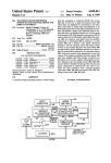
Figure 1 Example interface 2 The development of strategies for managing the emission of greenhouse gases from aviation
clearly need to be underpinned by a solid understanding of, and robust numerical data on, the
patterns of CO2 emitted by aircraft. At the present time most policy makers only have access to
high level fuel use data. For example, in Australia the Department of Resources, Energy and
Tourism publishes data on jet fuel sales at the National and State/Territory level
(http://www.ret.gov.au/resources/fuels/aps/pages/default.aspx). It also breaks this down into fuel
for domestic and international operations. While this is useful, it does not enable either the policy
maker or a member of the public to understand the drivers behind the macro fuel use figures – the
implications of proposed and/or actual expansions at airports, the introduction of new aircraft
types, the introduction of new services and/or routes, changing load factors, changing travel
demand patterns, etc.
In the absence of understanding carbon footprints at the disaggregated level there will be a danger
that decisions made both by individuals about personal travel, and by government decision makers
on long term strategies, may not achieve the optimum outcomes.
1.2
Design Concept
TNIP Carbon Counter has been designed in such a way as to facilitate transparency and to assist in
building trust in carbon calculations, both for decision makers and members of the public, by
allowing the user to drill down into ‘the workings’. In line with the TNIP noise applications
(http://www.infrastructure.gov.au/aviation/environmental/transparent_noise/tnip.aspx), the aim is
to get away from complex black box modelling techniques which effectively entrust knowledge to
the hands of a small number of technical cognoscenti. Key features of the design include:
ƒ
The model computes fuel use for departures only. This is designed to follow what appears
to be becoming standard practice – carbon footprinting on fuel uplifted in order to avoid
double counting.
ƒ
The use of readily available input data. The model uses the same time-stamped
airport/aircraft movement datasets that are used in TNIP noise applications, as well as
published airline schedules.
ƒ
The fuel burn data which underpins the fuel use calculations is transparent and easily
modified. The program comes loaded with the EMEP/CORINAIR fuel use dataset which
also underpins the ICAO Carbon Calculator.
ƒ
Being a macro tool the results are based on standard averaged data. The user needs to
be aware that fuel burn for ‘identical’ operations can and in most cases will vary,
sometimes widely, from flight to flight in the same manner that the noise received on the
ground from ‘identical’ aircraft operations varies.
ƒ
The user does not need specialist skills to rapidly interrogate data and produce reports.
The user is provided with tools to carry out simple ‘what-ifs’ and to produce reports
exploring the outcomes of different scenarios.
1.3
Potential Applications
TNIP Carbon Counter has a number of potential uses. The following list contains examples of
potential uses and is not intended to be exhaustive:
ƒ
Carbon footprint trend reporting (e.g. State of the Environment reports; regular
environment reporting).
3 ƒ
Environmental Impact Assessment – carbon footprinting the outcomes of proposed
developments (e.g. new aircraft types, new runways, flight paths, services, etc).
ƒ
Community consultation/engagement on airport operations and proposed developments.
ƒ
Responding to requests for carbon footprint information from, for example, elected
representatives, government agencies, researchers, students and members of the public.
ƒ
Briefing decision makers on the carbon implications of proposed actions.
ƒ
Policy development – examination of scenarios, what-ifs, etc.
ƒ
Analysing trends in efficiency – developing and reporting key performance indicators
(KPIs).
ƒ
Computing corporate carbon footprints or individual carbon offsetting.
ƒ
Examining options for travel at the personal level (e.g. type of aircraft, route, aircraft vs.
train, car, etc).
ƒ
Carbon footprinting of economic sectors (e.g. tourism, mining, etc).
ƒ
Computing the costs per head, and the quantum of funds that would be generated, under
varying carbon charging regimes.
4 Chapter 2
Quick Guide
2.1
Introduction
This part of the manual aims to provide the user with a quick tour of TNIP Carbon Counter without
expanding on the more advanced parts of the program. The full functionality of the Carbon
Counter is discussed in detail in subsequent parts of this manual. The program is released with
three accompanying sample datasets to enable the user to trial the software to gain a sense of its
capabilities.
A sample dataset for one month for Sydney Airport is loaded internally. This is the same
demonstration dataset that is made available with the noise versions of TNIP. To demonstrate the
network capabilities of the program, a synthetic one year dummy dataset for the Australian
network has been included in a demonstration data Vault.
A sample corporate dataset is also included to demonstrate the use of the Carbon Counter for
corporate footprinting.
2.2
Main Menu
When the program is started the user is presented with the main menu shown below. The first
three buttons:
,
, and
are associated with
the program setup elements of the software.
Figure 2 Main Menu – Sydney vault loaded and March 2003 data movements active Setup
The program is released with sample airport and aircraft setup files already loaded. The user does
not need to delve into this part of the program in order to view the output from the program.
However, if the user wishes to view details of the airport/s, aircraft types and fuel burn profiles in
5 the program, then clicking on the first three buttons will enable exploration of the contents of these
setup files. The functions underlying these buttons are described in detail in Chapter 3 of this
Manual.
The next button
is associated with loading data (see Chapter 5). The
button takes the user to the archive folder structure of the loaded
data as discussed in Chapter 4.
Analysis and Reporting
The remaining two buttons are for analysing the aircraft movement data and computed carbon and
for producing output in the form of graphics or exported data. The
button enables the user to examine subsets of the loaded and computed data by applying filtering
tools (see Chapter 8 for further details).
The
button allows for detailed carbon footprint analyses to be
made for departures from a user selected individual airport and is discussed in Chapter 11.
2.3
Queries and Reports
This facility is network based rather than being single airport centric. The interface enables the
user to compare various parameters (e.g. number of aircraft operations, fuel usage, carbon
emissions, distance travelled, total passengers) for various categories or groupings that have been
filtered from the main datasets using the program’s filtering tools (see Part III). The
Queries & Reports window, shown in Figure 3, is accessed by clicking the button with the same
name on the Main Menu of the program (Figure 2).
1
B
A
2
3
C
Figure 3 Network Carbon Overview ­ Movements tab 6 When movement data is loaded into the program using the Data Input & Pre-processing
screen (refer Chapter 5), airports and their corresponding movement data are placed inside a user
selected folder inside the ‘Vault’. The list at [A] shows folders in the Vault that have been used to
store airport and aircraft movement data. Selecting a folder changes the details in the lists at [B]
and [C] to reflect the information relating to the selected folder.
The user can breakdown aircraft operations into categories or groups using a filtering tool called
‘Save Points’. Save Points are, in effect, stored queries that can be used to carry out data
disaggregation and filtering (see Chapter 7). The Save Point groups previously created by the user
for the movements in the folder selected are shown at [B] along with a breakdown of the
movement numbers, fuel usage, calculated carbon, distance and passenger statistics for each Save
Point group available.
Clicking one of the Save Point group entries in [B] shows the computed results for individual Save
Points in that grouping in the Overview Breakdown list at [C]. The details in this list will also show
Save Point breakdown for movement numbers, fuel usage, calculated carbon, distance and
passenger statistics.
The example in Figure 3 shows the ‘By INT/DOM’ Save Point selected in [B] which breaks the
results down into contributions from the domestic and international sectors as shown in [C].
Clicking on the ‘Export’ button [2] copies the results to an Access datasheet which the user can
then copy to another application.
Clicking the Reports tab at [3] enables the user to see the results expressed in additional metrics
for the chosen operational grouping (Figure 4). This is similar to the Reports tab in the
Active Movements window of Figure 7.
A
B
1
Figure 4 Network Carbon Overview ­ Reports tab 7 Various metrics can be selected in the listing at [A] which are then plotted and listed in [B]. The
data can be copied to other applications (e.g. Microsoft Access, Excel, etc) by clicking the ‘Copy
Data’ button at [1] to facilitate further analysis and the generation of more complex graphics. A
more detailed description of the Queries & Reports window is discussed Chapter 8.
2.4
Active Movements
Detailed single airport based analysis is carried out through the Active Movements interface. To
open the interface select the
button on the main menu (the button
name will change depending upon whether an airport movement has been made active in the
Vault). This brings up the Carbon Counter main interface that initially opens at the Movements
tab [1] (Figure 5).
All movement sets loaded into a vault can be viewed by the Active Movements interface;
however, to analyse a movement set it must first be made active. For a description on how to
activate a movement set refer to Subsection 4.5.1.
This part of the program provides the user with the capability of drilling down into the data for an
individual airport.
2.4.1
The Movements Tab
The Movements tab [1] of the Active Movements screen (Figure 5) contains three main areas,
show as [A], [B] and [C] in Figure 5, are discussed below.
B
1
2
A
Figure 5 Carbon Counter Movements tab interface C
ƒ
[A] The Data Section provides a window on the listing of the aircraft movements in the
active dataset (see Subsection 5.4.2 for an explanation of ‘active dataset’).
ƒ
[B] The Calculation Factors Section lets the user enter a value for the load factor, the
price of carbon and the RFI (Radiative Forcing Index – a factor to take account of the
non-CO2 climate change impacts of aviation). The GCD (Great Circle Distance ) factor can
be used to represent the actual average distance flown between two ports which in
8 practice will be greater than the GCD (e.g. due to the structure of air routes). TNIP
Carbon Counter uses the ICAO Carbon Calculator GCD adjustment factor. Further details
can be found on page 8 of the ICAO Carbon Emissions Calculator Methodology
(http://www2.icao.int/en/carbonoffset/Documents/ICAO%20MethodologyV3.pdf).
ƒ
[C] The Fuel & Emissions Statistics Section displays a range of information relating to
individual and aggregated movements. The individual, aggregated and/or average trip
statistics reported relate to various details such as trip distance, fuel burn, movement
counts, fuel and carbon emissions for the whole of a trip and also for the average trip and
on a per passenger, and on a per passenger per 100 kilometres, basis. Several of the
emissions statistics are also given a monetary unit based on the carbon price entered by
the user in the Calculation Factors Section. These statistics are also affected by the
Aircraft Load Factor and the RFI entered.
After setting the calculation factors [B], the user can step through the listing of movements shown
in the data window [A]. The fuel/carbon/offset information for the flight highlighted in the data
area is shown in the top of the Fuel & Emissions Statistics section in the boxes at [C] which lets
the user rapidly learn about the carbon footprint of specific aircraft types on selected routes.
Also present in section [C] are aggregated trip statistics for all trips in the currently active
movements (under the title Trip Details and Per PAX) as well as aggregated trip statistics for a
selected Save Point (under the tile Filtered Trip Distance).
2.4.2
The Aircraft and Airports Tab
Selecting the Aircraft and Airports tab ([2] in Figure 5) brings up the Aircraft and Airports
display shown in Figure 6. This is similar to the Movements tab except that this tab now shows an
aggregated version of the aircraft movements file. This allows the user to step through the dataset
at either the aircraft type or airport level (as opposed to the movement by movement level on the
Movements tab). Each selection provides fuel/carbon/cost information in the window at [C] as
before.
6
1
C
4
5
3
2
Figure 6 Aircraft and Airports tab 9 Running a Carbon Count
To this point information has been shown for average individual flights, aircraft types or routes. All
the data can be aggregated by selecting the
button at [1] that is located in the
Calculation Factors section. When this is selected the program progressively sums up the
information about each operation in the aircraft movements file. During this process a progress
bar appears at [2] and information on the count is progressively updated and shown in the area at
[3], in the dotted area at [4] and, if a Save Point is selected, at [5]. The count can be
interrupted at any point by clicking on the ‘click to pause’ box that appears in the middle of the
screen during the counting process. Counting can be restarted by selecting the play button
button when counting is interrupted (see which automatically appears next to the
Section Part IV11.4 for details).
The information shown in the boxes at [4] relates to the whole of the active dataset. Subsets of
the main database can be readily selected via the use of Save Points (see Section Part III7.2).
When a subset is selected, parallel information for the subset is shown in the box at [5]. This is a
very useful and powerful tool for generating comparative disaggregated carbon footprint
information.
2.4.3
The Reports Tab
Selecting the Reports tab ([6] in Figure 6) brings up the screen shown in Figure 7.
This screen has four key areas: the metrics list [A], the data selection area [B], the graphics area
[C] and the data area [D].
B1
C
A
B
D
2
3
1
5
Figure 7 Reports tab ƒ
4
[A] Metrics List – this area contains a listing of different metrics for examining the data
in the selected dataset or sets. One or any number of the metrics can be selected using
the mouse and the control or shift key. When the user initially opens this tab the metrics
operate on the active dataset – other datasets can be used, and comparisons between
datasets can be made, through the data selection area.
10 ƒ
[B] & [B1] Data Selection Area – these areas let the user select subsets of the active
dataset and select a number of datasets through drop down lists, boxes and radio buttons
- this is explained in detail in Section Part IV11.5. When one or more Save Points have
been selected from the list in [B] computation is initiated by pressing the Show Report
button at [1]. The report is then shown in the graphics area.
ƒ
[C] Graphics Area – this area gives a graphical display of the results of the computation
where the selected metric(s) have been applied to the selected data. The form of the
graphic (e.g. pie chart, histogram, etc) can be presented in a number of ways by selecting
from the drop down list and boxes at [2]. When the program has generated a graphic it
button [3] – this places
may be exported to other programs by selecting the
the graphic on the clipboard which then lets the user for example, paste it into a report
being generated in Microsoft Word.
ƒ
[D] Report Data Area – this area contains the data underlying every graphic. This data
button [4] – in a similar
can be exported to another program by selecting the
manner to the graphics area, this data is placed on the clipboard to facilitate its use in
other programs (e.g. Excel).
The program also contains a number of embedded reports which can be generated by selecting
from the drop down line list at [5].
2.5
Summary
This brief guide has been intended to demonstrate the broad capabilities of the program using
sample airport and network datasets. The following parts of this manual provide a detailed
description of how the user can set up the program, load data and carry out detailed footprinting
analyses.
11 12 Part II
Data Management
13 Chapter 3
Program Setup
3.1
Getting Started
To perform carbon counting a number of key setup steps must be performed. The two key areas
are Airport and Aircraft setup. When these areas have been set up, airport movement data can
then be imported and carbon counts can be run.
Airport setup involves, amongst other things, identifying the latitude and longitude of each airport
in the movement file. These airport configurations are used to calculate the trip distances and are
stored in a single Airport text file.
Aircraft setup, amongst other things, involves the use of two setup files. Rather than providing the
fuel burn characteristics for individual aircraft, similar aircraft are grouped together and common
fuel burn characteristics are used for each grouping. These aircraft groupings, or substitutions, are
the basis of the Aircraft (Substitution) text file and use reference aircraft types with known fuel
burn characteristics and are substituted for the actual aircraft used in the movement file. Once the
substitutes are defined the fuel burn characteristics for each substitute must be set up. The
aircraft substitute fuel burn is stored in the Fuel Burn file.
A
A B
B
Figure 8 Main Menu showing Advanced Setup For the sake of simplicity the main menu has been designed to provide quick access to the loading
and setup of Airports [A] and Aircraft [B] via the first two buttons on the main menu:
and
respectively.
It is also possible to access these interfaces by selecting the
button on the main
menu and then pressing either of the first two buttons on the Advanced Setup menu (Figure 8):
[A] or
[B].
14 3.2
Airport Set Up
The first part of the carbon calculation process involves the calculation of the distance for each trip.
While it is possible to make changes to airports on an individual basis it may be easier, particularly
when changing two or more airports, to make these changes directly to the text based Airports file
and then load the updated Airports file into the system.
3.2.1
Airports File
The Airports file contains information on all the airports currently referred to in the Origin Airport
and Destination Airport fields of a movements file. The format of the Airports file is shown
below in Figure 9. Column headings in the first line are optional; however, the order of the data
columns is compulsory. While data column names are not necessary they are useful for the user
and are recommended.
Figure 9 Sample Airports file ƒ
Column A: Shows a sequential ID for the airport. This will not be used at load time and
is a number generated by the system when airports are exported.
ƒ
Column B: Lists the ICAO airport codes (4 characters) which appear in the aircraft
movement data file.
ƒ
Columns C & D: Respectively these two columns show the latitude and longitude of each
of the airports in degrees (DD), minutes (MM), seconds (SS), milliseconds (optional) and
direction [Dir] and is in the format of DDMMSS[Dir] with a single letter for the direction
[Dir] as either N/S or W/E.
ƒ
Column E: Shows the airport name and may be up to 50 characters in length.
ƒ
Column F: Is for assigning the airports to various time zones. This information is
currently not utilised in the program and can be left blank.
ƒ
Column G: Assigns the airports to any geographical allocation of the user’s choice. For
example, the user may wish to categorise the airports according to regional jurisdictions
(e.g. States, Provinces, etc), and individual countries or geopolitical regions (e.g. North
15 Asia, South East Asia, etc). Choosing ‘Save Points’ (explained in Chapter 7) with ‘State’ in
the name will organise the results into the ‘State’ groupings defined in this column.
ƒ
Column H: Records the runway type of the airport (e.g. asphalt, concrete, dirt, etc).
ƒ
Column I: The IATA code for the airport. If a movement file to be entered uses IATA
airport codes this information is used to translate them to ICAO codes.
The program uses the information in this file to compute the great circle distance between the
origin and destination airports for each aircraft movement loaded from a movements file.
3.2.2
General Airport Details
To load an Airports file or edit or view the individual setup for a specific airport select the
button on the main menu to bring up the interface in Figure 10.
While it is not possible to load Airports files directly from this screen, this can be achieved by
button at the bottom of the screen and using the subsequent
selecting the
interface to load a file. By default the current airport will be displayed and is dependent upon the
currently active movement set.
Subsection 3.2.4 Subsection 3.2.3 Figure 10 Edit Airport Setup interface The General Airport Setup screen asks the user to enter the name of the current airport, its
ICAO code, the Airport IATA code, the state and runway type of the airport and Aerodrome
Reference Point (ARP) in latitude and longitude. The user can also input the ICAO code for one or
a number of countries that the program then treats as domestic airports. Doing this enables the
program to differentiate between domestic and international operations when counting carbon and
enables international and domestic Save Point creation and searching.
The ARP information is needed in order for the program to calculate the distance, and hence, fuel
use and CO2 generated by each movement.
The user may work in decimal notation. The program calculates the latitude and/or longitude in
the format DDMMSS[Dir] for Latitude and DDDMMSS[Dir] for Longitude. DD & DDD = Degrees,
MM = Minutes, SS = Seconds and [Dir] = 1 character representation of the direction; Latitude =
N(orth) or S(outh); Longitude = E(ast) or W(est).
3.2.3
Currently Loaded Airports & File Loading
Selecting the
button on the Edit Airport Setup screen (Figure 9) provides the
user with the ability to examine and edit the currently loaded airport details. From this screen it is
also possible to load details from an existing Airports file.
16 Figure 11 Loaded Airports interface Edit Existing Details
There are two methods for editing the details for an airport. To quickly change the airport name or
its latitude and/or longitude via the Loaded Airports interface (Figure 11) first select the desired
airport from the list, modify the appropriate fields and then press the
button.
Alternatively, highlight the airport to be changed and then press the
button to edit the
airport details via the General Airport Details screen.
Load Airports Files
To load an Airports file click the
(Figure 12) click the
button and, from the Data File Setup interface
button at the top of the interface. Navigate to the file to be loaded and
then press the Open button.
Figure 12 Airport Data File Setup interface On loading an Airports file, if any airports in the currently loaded movements have not been
defined the user will be prompted with details of the undefined airports and given the option to fix
them before continuing.
17 The last step in loading the Airports file is the updating of the ‘Individual’ airport details stored in
the Vault. The last prompt allows these airports stored in the Vault to be updated with the
contents of the Airports file or left unmodified by not updating the ‘Individual’ Vault airport details.
For large Vaults this process may take a while and if it is known that no airports in the Vault differ
from the airports file this step can be avoided. However, in general, it is best to select ‘Yes’ to this
prompt to ensure vault consistency unless there is a specific reason not to.
Exporting Airports Files
It is also possible to have the Carbon Counter generate an Airports file from the currently loaded
airports. This is particularly useful when changes are about to be made to the loaded airports and
a backup is required. If the current Airports file is missing, the export facility provides an excellent
means of providing a replacement file.
To export the current airports simply click the
button located underneath the
button in Figure 11.
3.2.4
Undefined Airports
button on the General Airport Setup screen (Figure 9)
Selecting the
generates the Undefined Airports screen that is similar to the Loaded Airports screen. The
Undefined Airports screen (Figure 13) enables the user to set up airports that are contained in
loaded movements but the program integrity checks have revealed as undefined in the loaded
airports.
The box on the left [A] shows the airports
in the loaded movements file that are not
contained in the Airports file. The user can
add these undefined airports to the
Airports file by using the cursor to select
one or more of these airports, enter the
airport name(s), latitude and longitude,
and then select the Define Permanently
button
at [2]. Alternatively,
the airport can be defined for the currently
loaded data by selecting the
A
1
2
button at [1].
Figure 13 Undefined Airports interface 18 3.3
Aircraft Set Up
This section provides the core information that enables the program to compute the fuel burn for
each individual operation.
3.3.1
Aircraft (Substitute) File
The format of this file is shown in the adjacent example. While it is not necessary to have field
names in the first line of this file, it is important to have the four columns of data in the correct
order. The four fields include:
ƒ
Column A: contains an aircraft type code
(maximum six characters) that is used to
compare against the aircraft type in the
aircraft movements file.
ƒ
Column B: contains a single character
which represents one of three aircraft types
– ‘J’ for jets, ‘P’ for non-jets and ‘O’ for
others (usually helicopters or other
unidentified aircraft).
ƒ
Column C: contains the CORINAIR
substitute aircraft code that is one of the
aircraft types in the Fuel Burn file discussed
in the next Section.
ƒ
Figure 14 Aircraft (Substitution) File Column D: contains the number of seats
for each aircraft type.
The program uses the data in the aircraft file to differentiate between jet and non-jet aircraft when
generating filtered datasets, for setting up auto substitutions and in determining the number of
seats for computing statistics on a per passenger basis.
While it is may be easier to make aircraft substitutions changes via the Aircraft Substitutions
interface seen in Figure 16 it is possible to make these modifications in the Aircraft (Substitute) file
and reload the file.
3.3.2
Fuel Burn File
The Fuel Burn file seen in Figure 15 is used by the program for setting up the fuel burn
characteristics of the various CORINAIR aircraft in Column C of the Aircraft (Substitutions) file (see
Figure 14). The Fuel Burn file can be set up and edited using the En-route Fuel Burn interface
(Figure 19) discussed later in this Part. The program also comes with a sample Fuel Burn file.
19 Figure 15 Fuel Burn File When editing fuel burn it may be easier to edit the fuel burn text file directly and then reload the
file rather than using the interface, particularly when the entries for two or more aircraft
The file may consist of up to 20 or more fields. While an absolute a minimum of four columns are
required multiple fuel burn columns are highly desirable. The loaded fuel burn uses 16 columns:
ƒ
Column A: AircraftSubstitute: the name of the CORINAIR substitute.
ƒ
Column B: PAX: the number of seats for each aircraft type.
ƒ
Column C: AircraftSubstituteID: the internal ID for the aircraft substitute.
ƒ
Column D onwards: Fuel Burn (kg/nm)
Each column covers a minimum and maximum distance which are used to compute fuel
burn based on the gate-to-gate trip distance.
The data item in each column represents fuel burn per nautical mile at the column’s
maximum distance. When the actual trip distance falls between a column’s minimum and
maximum value a straight line interpolation is made between that column’s value and that of
the previous column.
Column names have three parts:
Part 1
minimum (nm - 5 digits)
Part 2
-
Part 3
maximum (nm - 5 digits)
Example Fields: 00000 - 00125, 000126 - 00250, 00251 - 00500, 00501 - 01000
Note the following: There is no space required before or after the hyphen. The range (or
band) of each column does not have to be the same for all columns. Each distance range must
be unique - a distance cannot fall under more than one column heading.
While the Aircraft (Substitute) file can be given any name the Fuel Burn file must be called FB.CSV
and must be located in the same directory as the Aircraft (Substitute) file. When an Aircraft
(Substitute) file is loaded, the program automatically looks for the FB.CSV file.
3.3.3
The
Currently Loaded Aircraft Substitutions and File Loading
button on the Main Menu brings up the Aircraft Substitutions interface at
Figure 16 which can be used to view and edit the current aircraft substitutions; automatically reset
the current substitutions as defined in the Aircraft (Substitute) file; or open the
Enroute Fuel Burn interface (Figure 19).
20 Additionally, this interface can be used to load the two aircraft setup files. To import both the
aircraft (substitution) file and the Fuel Burn file use the
button. The current
substitutions and fuel burn can be exported using the
button.
Edit Existing Aircraft Substitution Details
To edit an aircraft substitution the user selects an aircraft type in the ‘Generic Aircraft Group’ list
[1] and then, if appropriate, selects an aircraft type or types from the ‘Available Aircraft’ list [2]
button at [3]. The list of aircraft
and adds this as a substituted aircraft by use of the
substitutes linked to the highlighted generic aircraft is shown in the box on the right. Aircraft can
be removed from this list by using the
button [4].
6
3
1
4
2
Figure 16 Aircraft Substitutions interface 5
When a new aircraft type is brought into service, such as the B737-800, and none of the existing
aircraft types in the CORINAIR dataset can be realistically used as a substitute, the user may create
a new substitute group by clicking the
button and entering the name of the new
button. When
group. Groups can also be renamed via this interface with the
deleting a group, substitution information for the group will also be deleted and all aircraft involved
in the deleted group will become available in the ‘Available Aircraft’ list.
Finding and Adding Aircraft
If an aircraft is to be substituted, however, the particular aircraft was not in the loaded Aircraft file
and does not exist in the currently loaded movements it is still possible to add this unlisted aircraft.
Select the group in the ‘Generic Aircraft’ list and then click the button at [5] situated
between the Available Aircraft list on the left and Substituted Aircraft list on the
right. Follow the prompts to either find an aircraft or, if cannot be found, add it to the
substitutes list.
No of Seats
When carbon is counted the number of seats assigned to an aircraft is taken from the aircraft file.
When an aircraft in the aircraft file does not have the number of seats defined the value in the field
at [6] will be used.
The number of seats defined in the field at [6] is initially supplied by the Fuel Burn file. It can be
manually overridden, however, every time a fuel burn file is loaded this value will be reset to the
value in the Fuel Burn file that is loaded.
21 Import Aircraft (Substitute) and Fuel Burn Files
To load both the Aircraft (Substitute) file and the Fuel Burn file open the Aircraft Substitutions
interface (Figure 16), click the
button to display the Data File Setup interface
(Figure 17) and then click the
button at the top right of this interface.
Figure 17 Aircraft Data File Setup interface Navigate to the Aircraft (Substitute) file to be loaded and then press the Open button on the file
dialog box. This will cause the aircraft in the file to be loaded. It is necessary to select an
Aircraft (Substitute) file even if only the Fuel Burn file needs to be reloaded.
Undefined Aircraft
The loaded movements are first checked to determine if any
aircraft not defined in the Aircraft file have been loaded. If any
undefined aircraft exist, a message advising of the undefined
aircraft will be displayed and the option given to correct the
problem aircraft. If the user selects Yes, the
Undefined Aircraft interface will be displayed (Figure 18)
where the user can define any unidentified aircraft shown in box
[A]. The user can select these individually or use the shift and
control keys to select common groups that can be defined by
clicking on the appropriate button at [B]. Depending on the
B
C
A
D
selection at [B], clicking on the modified button at [C] (either
,
or
) will define the selected
aircraft to the relevant type temporarily - for the current allocation
process only. Depending also upon the selection in [B], using the
Figure 18 Undefined Aircraft interface relevant button at [D] writes the selected aircraft types to the Aircraft (Substitute) file and makes
the change permanent.
Fuel Burn
When undefined aircraft have been dealt with, a check is made for the presence of a Fuel Burn file.
If a Fuel Burn file (FB.CSV) is found at the location containing the Aircraft file, the user will be
22 prompted to confirm replacing the currently loaded aircraft substitution fuel burn specifications
with those found in the file just found. If Yes is selected the current details will be overwritten.
Substitutions
Next the user will be asked to automatically define the substitutions for the aircraft being loaded
with the setting as defined in the Aircraft (Substitute) file. Clicking Yes will load the aircraft and
set up the substitutions based on the file settings. Clicking No at this stage will still load the
aircraft, however, current substitutions will not be altered.
Once the process to automatically define the substitutions has been completed, a message will be
displayed showing the aircraft types that were substituted.
This completes the loading of both the Aircraft (Substitute) file and the Fuel Burn file.
This interface can also be accessed via the Airport Setup Menu by selecting the
button (Area B in Figure 8).
3.3.4
The
Edit Existing Fuel Burn Data
button on the Aircraft Substitutions screen (Figure 16) brings up the
Enroute Fuel Burn interface shown in Figure 19. This interface can also be accessed from the
button on the Advanced Setup screen shown in
Figure 8.
3
2
1
Figure 19 En­route Fuel Burn interface This interface is very important to the functioning of TNIP Carbon Counter as it is used to store
both PAX information and fuel burn parameters for each CORINAIR aircraft type.
Seats
For each generic aircraft type, the user is required to enter the number of seats. If no seat
information for an aircraft is included in the Aircraft (Substitutions) file (see Figure 14 column D
titled: SEATS) the value displayed here [3] in the En-Route Fuel Burn screen (Figure 19) is
used by the program to compute the ‘per passenger’ metrics output by the program.
23 Fuel Burn
The fuel information is entered in the form of a fuel consumption rate for a series of discrete
ranges each with a minimum and maximum distance. As discussed in Subsection 3.3.2 the data in
these columns indicates the absolute fuel burn in kilograms per nautical mile (kg/nm) for the
maximum distance covered by the range of the column.
The fuel burn per nautical mile for all distances in a range, other than the maximum, are
interpolated based on the maximum of that range and the previous one.
Each distance range is unique and no distance can be allowed to be covered by more than one
column.
The default information that has been entered into the program has been extracted from the
EMEP/CORINAIR dataset (see Appendix A) where the EMEP/CORINAIR fuel burn values have been
converted from a total fuel burn amount (for the band’s maximum distance) to a fuel burn per
nautical mile figure for that distance.
Selecting the
button at [1] in Figure 19 brings up the Microsoft Access table
show in Figure 20 .
Figure 20 Sample Fuel Burn Report This shows the table sitting under the previous interface and facilitates making a rapid fuel burn
cross comparison between different aircraft types.
The
button at [2] in Figure 19 gives access to the interface at Figure 21.
Figure 21 Default Fuel Burn Intervals interface 24 This lets the user enter the bounds of the distance ranges. It also lets the user set up distance
bands in the form of ‘Stage Lengths’ (this enables, for example, the user to set up distance zones
which are common to those used in the FAA’s Integrated Noise Model (INM)). This facilitates, for
example, the use of common datasets for assessing both aircraft noise and carbon footprints in
environmental assessments (see Section 12.3 Example 3: Environmental Impact Assessment (EIA)).
3.4
Other Settings
button on the main menu brings up the Advanced Setup menu displayed
The
in Figure 22. This sub menu can be used to edit setup data for five separate areas of the Carbon
Counter.
Figure 22 Advanced Setup The first three buttons were addressed above in the sections on Airport Setup and Aircraft Setup.
was discussed in Subsection 3.2.2 and is also accessible
from the main menu.
was discussed in Subsection 3.3.3,
was discussed in
and is also available from the main menu.
Subsection 3.3.4 and is accessible from the Aircraft Substitutions screen by clicking the
button.
The remaining two buttons are discussed in the following two Subsections.
3.4.1
Missing Aircraft Defaults
In some datasets the aircraft field for an entry in the movements file may be missing. In these
circumstances the program will calculate the fuel use (and hence carbon) for these operations
using a substitute aircraft type. This substitution, known as the Missing Aircraft Defaults is
based on the distance that is travelled by the unknown aircraft during the identified movement.
Pressing the
button on the Advanced Setup menu opens a
Microsoft Access table listing the default aircraft to be used in these circumstances. The initial
settings for the default aircraft can be seen in the
table at Figure 23. By default, three distances
bands in kilometres are initially set up (0-1000,
1001-5000 & 5001-20000) with each band set to
small (DH8), medium (B737) and large (B747)
Figure 23 Default (Unknown) Aircraft 25 aircraft respectively.
Specifically, the Missing Aircraft Defaults are used by the Data Input & Pre-processing
interface when loading movement data and when an entry in the column specifying the aircraft
type is missing and not known.
The table is organised so that a band of distances is supplied in a From and To column. Each of
these bands has an aircraft associated with it. When data is loaded via the
Data Input & Pre-processing screen each movement that does not have an aircraft will not
have trip distances calculated unless the Data Input & Pre-processing checkbox
(
) has been checked and the Missing Aircraft Defaults entries have been setup.
3.4.2
Time Periods
Pressing the
button on the Advanced Setup menu opens the
Edit Time Periods interface, which can be used to create or edit the time ranges used by time
based Save Points and reports.
3.4.3
Carbon Count Factors
To access the factors used for carbon counting press the
button
on the Advanced Setup screen. You will then be presented with the screen shown at Figure 24.
This screen is used to modify three different options: The unit and price of carbon per tonne; the
specific gravity (SG) of fuel which is used to convert kilograms into litres; and the fuel to carbon
conversion factor which is used to compute the amount of carbon produced from a kilogram of
fuel.
Figure 24 Carbon Count Factors screen 3.4.4
RTK
Computations of revenue tonne kilometres (RTK) requires the adoption of a number of factors.
The RTK screen show in Figure 25 enables the user to input the parameters which are used to
calculate RTK.
To open the RTK screen (Figure 25) press the
button on the
Advanced Setup screen. There are two sections to this screen, both of which are needed to
compute the freight weight component of the RTK calculations. The top section has a single field
and is used to enter the average weight per passenger in kilograms. The next section contains five
fields which deal with the percentages of passenger to freight weights for the three stages of flight;
short, medium & long haul.
The field in the first section is used to enter the average
weight of each passenger including all baggage they have.
Calculating the ‘Total Weight of all Passengers’ involves
calculating the total number of passengers – ‘load factor’ by
‘number of seats’ by ‘number of flights’ - and multiplying this
by the number supplied in the field. The number here is
represented in kilograms.
Figure 25 Setup screen for RTK 26 By knowing the ‘% of the Total Payload’ attributed to passengers we can work backwards from the
known ‘total passenger weight’ to arrive at the ‘Total Payload’. By subtracting the ‘total passenger
weight’ from ‘Total Payload’ we arrive at the ‘Total Freight Weight’. All RTK calculations can now be
performed.
27 Chapter 4
The Data Vault
4.1
Introduction
Once the airport, aircraft and other key parameters have been set up, a data vault has to be
generated.
The Data Vault is the archive for the aircraft movements datasets that are loaded into the program.
Establishing a vault minimises the time taken to load files and assists in avoiding mismatching
errors. This is achieved by archiving all the relevant files in a prepared format that enables the
user to switch rapidly between the archived movements.
TNIP Carbon Counter is designed to be capable of storing and processing very large databases
(millions of movements at thousands of airports). The data vault avoids the 2 gigabyte file size
restriction inherent in Microsoft Access by breaking down the data into ‘bite size pieces’ that can be
handled by a standard personal computer.
The main functions of the Data Vault are to provide a central data repository which enables the
user to:
ƒ
Set up multiple airports with different parameters for each one.
ƒ
Load one or more movement files into each airport and then quickly view the movements
in each loaded movement set.
ƒ
Build, store and retrieve multiple Save Points for each movement file loaded.
ƒ
Automatically restore all the relevant airport details and Save Points when activating
movement sets.
ƒ
Analyse the data from one or more of the movement files individually or combined into
various subsets.
In effect, the Vault is a repository for storing and quickly retrieving a large number of aircraft
movement files for one or a large number of different airports and archiving them using a simple
tree style interface. The number of airports and movements that can be contained in a Vault is
basically only limited by the amount of available hard disk storage space. After one or more
aircraft movement files are loaded the last one loaded will be automatically made the ‘active’ file.
The user is able to switch the active movements at any time. Additionally, the program allows
multiple Vaults to be set up with different airports, movements and settings specific to themselves
and independent of other vaults.
Prior to loading data the user must have prepared all the necessary setup data files as described in
Chapter 3.
4.2
The Vault Interface
Selecting the
button on the main menu (Figure 8) brings up the
interface shown in Figure 26.
28 1
4
3
2
5
11
7
6
10
9
8
Figure 26 Data Vault interface The address of the current Vault is shown at [1]. Other Vaults can be located using the browse
button
at [2] or new Vaults can be created by selecting the
button at
[3].
Clicking the New Vault button [3] brings up the Create New Vault dialog box shown in
Figure 27 which allows the user to create three different Vault types.
1 2 3 4 6 5 Figure 27 Create New Vault dialog By default, the Standard Vault [2] is created for reading in a standard TNIP aircraft movements
data file. Checking the Non Standard Vault option [2] allows the user to set up two other vault
types: (i) an Industry Mode vault [3] where the data input files contain the actual fuel use per
flight or (ii) a Corporate Mode vault [4] where the input files contain travel data for a company’s
employees. The format and types of input data are discussed in Section 5.2.
29 For each of the three Vault types, the user then needs to select whether the Vault will contain
aircraft movement files where each line in the files represents (i) a single aircraft operation [5] or
(ii) a number of aircraft movements [6].
Returning to Figure 26, when the user browses for existing data Vaults, the program will perform a
scan from the selected location and display a list of available Vaults in the dropdown list [4] where
the user can then select an appropriate one from this list. Alternatively another location can be
browsed to find additional Vaults using the
button. When a valid Vault has been selected and
the Vault is opened this list will contain only one item – the current Vault. To populate this list
again perform another browse. If, after a browse operation, only one Vault is found it is loaded
automatically.
During the loading process the program examines the data being loaded and checks its integrity. If
a Vault database is missing, corrupted or not in the correct format the program will attempt to
correct the problem and a message will be displayed informing the user of the problem and
whether the problem has been fixed.
When activating movement sets, the Vault attempts to avoid a number of potential problems
related to undefined aircraft types or airport codes. The carbon associated with movements in
undefined aircraft types or at undefined airports will not be computed and hence the carbon counts
will be under reporting. Therefore it is strongly recommended that the user completely work
through the data integrity checking processes initiated by the program during the activation
process. This is discussed in Subsection 4.5.3.
Please note the following definitions: the loaded movement file data will be referred to as
movements. When specifically referring to the movement container or place holder (see Vault
Structure Overview in Section 4.3) this manual will refer to them as a movement set, movement
container or simply container.
4.3
Vault Structure Overview
Both the airport and the movement container are stored and accessed via the tree structure in the
‘Airport Movements in the Vault’ list [5] from the Data Vault interface. Folders exist to help the
user further organise and group airports and movements. Adding a folder, an airport or a
movement container is done by selecting the
button [6]. This button brings up the
dialog box in Figure 28. When adding to the top level the Movements button is disabled.
Figure 28 Add to Vault dialog In summary the function of each item that can be added are:
ƒ
A Folder: Used as a simple folder-like container for one or more airports or movement
sets. These appear as standard yellow folders (
). Folders can be nested and
help to organise or document the tree by using clear and simple descriptions.
E.g. ‘The World’, ‘Australia’, ‘Asia Pacific’, ‘2000 Movements’ & ‘1990 Annual’.
30 ƒ
An Airport: Used to group together any number of movement datasets which are all
related to the same airport. These appear as yellow folders with a picture of a runway
(
). Details specific to the airport will relate to all movement sets loaded under it.
These details include: airport name, latitude/longitude and a listing of the ICAO country
codes prefixes for the airport.
ƒ
A Movement Set: This is the container (or placeholder) that is used to store actual data
for a movement dataset and cannot be created at the top level. These appear as an
aircraft to signify they are movements (
). The number of movements is
displayed in brackets. When activating a movement set, highlight the container and then
select the ‘Activate’ button [8] in Figure 26. Similarly, to perform other vault actions,
such as loading data, counting carbon, renaming or deleting movement sets, first select
the movement set and then click the relevant button. For more information on these
actions refer to the relevant parts in this chapter.
Airport
Folder
Movements
Figure 29 Vault tree structure The example above shows that ‘Sydney’ airport has been created (yellow folder with a runway
[Airport]) with two sub folders ‘1990 Annual’ and ‘2000 Annual’ (plain yellow folders [Folder]).
The ‘1990 Annual’ folder has two movement sets loaded under it: ‘1998’ and ‘1999’ (represented by
the aircraft [Movements]) having 282,893 and 280,341 movements respectively.
4.4
Loading Data into the Vault
Once a data vault is set up, the next step is to load data. The standard (and recommended)
procedure for loading data is to exit from the Data Vault interface and enter the Data input &
Pre-processing interface by selecting the similarly named button on the Main Menu (Figure 8).
This interface provides the preferred route for loading aircraft movement data sets into the
program. This is discussed in detail in Chapter 5.
However, the program does provide the user with the ability to load data for individual airports
from the Data Vault interface once a container (represented by an aircraft icon) has been set up. A
movement data file can be loaded into the container by highlighting the aircraft icon and selecting
the
button [7] on the Data Vault interface (Figure 26). This may be a useful shortcut
for experienced users.
Once data is loaded, the user can directly proceed to interrogating the data using the Queries and
Reports interface accessed via the Queries & Reports button on the Main Menu (Figure 8).
Alternatively, as discussed in the next section, data can be ‘activated’ and its integrity checked prior
to interrogation.
31 4.5
Activating and Checking Movement Data
4.5.1
Movement Activation
TNIP Carbon Counter provides two ways of storing, counting and analysing data: either directly
using the internal TNIP Carbon Counter tables or from movements inside the current Vault. The
internal tables are active when the program is first started, whenever no Vault movement has been
made active or when a problem exists with the current Vault which cannot be resolved
automatically. To identify the currently active Vault movement its name and reference is placed in
the title bar of various interfaces.
Once one or more files have been loaded into the Vault, return to the Data Vault (Figure 26)
and, after ensuring the proper movement container is highlighted press the Activate toggle button
[8]. Depending upon whether the movements are already active or not you may see either one of
the toggle buttons Figure 30 or Figure 31.
Activate
If the highlighted movement container is not already
activated the ‘Airport Setup’ button will be greyed out and
the Activate/De-Activate button below it will display the
word Activate as in Figure 30.
Figure 30 Activate Button (Activate)
Deactivate
If the highlighted movement container is already activated
the ‘Airport Setup’ button appears as normal and can be
selected and the Activate/De-Activate button below it will
display the word De-Activate as in Figure 31.
4.5.2
Figure 31 Activate Button (De­Activate)
Activated Movements
When a valid container is selected and made active, the title bar on various screens (including the
Data File Setup screen) will be modified to specify the name of the Vault, airport and movement
that is active. This is done by displaying each of these parts, separated by a colon, and then
enclosing them in braces {…}. The first part will be the Vault name: the second part will be the
airport name: the third part will be the movement container name.
The screen shot Figure 32 is an example from the Data File Setup screen and shows that the
March 2003 movement set for Sydney Airport from the Sydney Vault is currently active.
Figure 32 Window Title Showing Active Vault 4.5.3
Data Integrity Checking
The program provides two opportunities for identifying potential problems related to movement
sets and subsequent problems when performing a carbon count. This integrity checking occurs
when data is loaded and, by default, every time a movement set is activated.
32 Data Loading - Aircraft Integrity Check
During the loading of movement data, via the Data File Setup interface, if missing or undefined
aircraft types are detected the dialog in Figure 33 appears which enables the user to update the
aircraft type file.
Figure 33 Undefined Aircraft dialog Selecting Yes brings up the Undefined Aircraft screen (Figure 18). For a more in-depth
discussion of this refer to Subsection 3.2.4. This interface can also be displayed by clicking the
button on the Aircraft tab of the Data File Setup interface. (The Data File Setup interface
displayed in Error! Reference source not found. does not display the Aircraft tab therefore the
button is not visible).
Data Loading - Airport Integrity Check
If there are unrecognised airport codes in the loaded aircraft movement file the user is presented
with the dialog shown in Figure 34.
Figure 34 Loaded Movements dialog Selecting Yes from this dialog will bring up the Undefined Airports screen (Figure 13). For a
more in-depth discussion of this refer to Subsection 3.3.3.
Movement Activation – Undefined Integrity Check
Upon movement activation the program again checks to see if there are any unidentified
movements due to unknown aircraft or unknown airports. For large movement sets (e.g. 1 Year)
there will be a few seconds pause before the movement set is activated as the program checks
each movement against the airports and aircraft data files that have been loaded. If unidentified
movements exist, the Unknown Movements Summary interface is displayed in Figure 35.
From this interface the user can examine the undefined movements and identify which ones can be
fixed.
33 2
1
3
5
4
Figure 35 Unknown Movements interface There is a check box at the bottom of the Data Vault screen (shown in Figure 26) titled
Auto Test for Unknown which, by default, is turned on. If unchecked the program will not
perform validation during activation. For new movements, movements not activated for some time,
or where their integrity is otherwise unknown, it is recommended that this be turned on before
activating these movements.
Depending upon the number of unknown movements and why they are unknown the user will see
either one or both of the tabs displayed in the interface.
To view the actual movements that are unknown select either the Airports [2] or Aircraft [3]
tab, then click one of the entries in the list [4]. The Unknown Movements list on the right hand
side will be updated with the movements that are ‘unknown’ based on the airport or aircraft item
selected in the left hand list. Unknown airports and aircraft are surrounded by a ‘ * ’, e.g. * JET *
* * when blank.
The list on the left is ordered by the number of undefined movements pertaining to the group and
the list on the right is ordered by the date and time of the movements.
The title bar displays the total number of discrete undefined movements as a total [1] and as a
percentage of all movements loaded. This provides a quick assessment of the impact of all
undefined movements. Please note that the total number of movements in the tab titles (in the
screen shot: Airports 269 [2] & Aircraft 1,267 [3]) do not necessarily add up to the total number
of movements [1] displayed in the title bar since a single movement may have both an unknown
aircraft as well as an unknown airport – as a result adding these two numbers will result in possible
double counting.
Looking at Figure 35 an example of this can be found after JET is selected in the list on the left
[4] and, looking at the list on the right, the first item in the list [5] shows an arrival from an
unknown airport ( * * : blank) in the unknown JET aircraft ( * JET * : JET).
No editing or changing of the movements can be done from this interface. It is provided solely as
an aid to alert, identify and enable the user to determine which movements should be corrected in
order to eliminate undefined movements. To fix either undefined airports or aircraft refer to
Airport Set Up in Chapter 3 Program Setup.
34 4.6
Vault Maintenance
As the Vault is used, with files being loaded, carbon being counted and Save Points being created
and deleted the Vault may become fragmented, especially when disk space is limited or the
computer is accessing the disk while TNIP Carbon Counter is writing to the Vault. Over time this
fragmentation will negatively impact on the speed of the program. To optimise performance it is
important to ensure there is enough free space on the hard drive and it is defragmented regularly.
Optimising the Vault
Over time, as files are loaded and reloaded, carbon counting and Save Points creation and deletion
is performed, the vault will increase in size. Some calculated data is stored along with movement
data in order to speed up access to the data. When movement sets are deleted neither the
movement data nor the calculated data are removed until the Vault is optimised.
If a lot of work has been done with a particular movement set, carbon counting and Save Point
creation, the user will often find it is useful to optimise the Vault for that particular movement set.
When work has been done to many or indeed all of the movement sets then it may be best to
optimise the entire Vault.
If a Vault has hundreds of airports along with their related movements, this process can take an
hour or more to complete. Because of the potential time delays caused by optimising the Vault,
this process has not been automated and is up to the user to initiate.
If the program has slowed down or disk space is running low because of the Carbon Counter, it
may be necessary to optimise the Vault. This function can be accessed via the
button at
[9] on the Data Vault interface in Figure 26. The user will be prompted with a dialog asking if
they wish to optimise the highlighted movement set or the entire Vault.
Figure 36 Optimise Vault dialog Selecting Yes from this dialog will only optimise the currently highlighted movement set, in this
example ‘March 03’. Optimising a single airport entry is a relatively quick operation. If the user
chooses to optimise the entire Vault by selecting No they must then confirm this operation.
Figure 37 Optimise Vault confirmation dialog Depending upon the speed of the computer and if the Vault contains hundreds of airports and their
related movements the process of optimising the Vault could take a significant amount of time,
indeed, this process may take hours. During this time TNIP Carbon Counter cannot be used.
35 While it is possible to open two or more instances of the Carbon Counter and have each instance
connect to the same Vault the user should ensure that this does not happen while the Vault is
being optimised.
Analysing and Repairing the Vault
During normal use of the Vault the program will check for inconsistencies and anomalies in the
Vault and attempt to correct these problems without intervention from the user. To search for and
correct all problems every time a Vault operation is done would slow things down too much;
therefore automatic analysis is limited to basic checking only.
If problems are experienced with the Vault, particularly if an old Vault is being used after
performing an upgrade of the program, it is strongly recommended that a Vault analysis be
performed. More extensive checks will be made and it is possible that old Vault files which have
out of date or obsolete data structures may be corrected and rendered usable.
It is recommended that the Vault is backed up first as this process makes actual changes to the
structure of the Vault. If problems occur (such as power loss) during this ‘analysis and repair’
process, parts of the Vault may be left in an unusable state. When ready to proceed the user must
open up the Data Vault interface and click on the
button at [10].
There are two types of analysis that can be performed, a fast analysis and repair, and a deep
analysis and repair. Clicking the
button will cause the first dialog, as displayed at
the top in Figure 38, to prompt the user with the name of the Vault being analysed and a warning
that a deep analysis and repair may take a long time. Clicking the Yes button on this dialog
performs a deep analysis and repair, whereas clicking No performs a quick analysis and repair only.
Upon clicking either Yes or No a subsequent dialog (see the bottom two dialogs also displayed in
Figure 38) will ask if Vault optimisation should also be performed as part of the Analysis and
Repair.
Figure 38 Analyse Vault dialogs As with Vault Optimisation, this process may take a significant amount of time and neither the
program nor the Vault can be used during this process. While it is impossible to predict the amount
of time required (as this is dependent upon the size of the Vault and the number of problems), as a
very rough guide this process may take anywhere between a minute for small vaults with few
airports to a few hours for large ones with hundreds or thousands of airports and movements. This
process cannot be interrupted.
36 During this process the user will be prompted with various dialog boxes regarding the state of the
Vault and any work that needs to be done. Problems that occur during this stage may be fixed
automatically or may require user intervention to correct them.
37 Chapter 5
Data Input and Pre-processing
5.1
Introduction
This part relates to the loading and management of the datasets that form the basis for the carbon
calculations and reporting carried out by the program.
TNIP Carbon Counter computes carbon footprints across an aviation network, or for a number of
aircraft operations, through aggregating the CO2 computed for each individual operation within a
dataset. The data required is relatively simple and the datasets that are used to perform the
footprinting are commonly generated within the aviation industry.
5.2
Aircraft Movements File
The aircraft movements file is a comma-separated text file and contains one line of data for each
aircraft movement. The Data File Setup interface, as discussed in Section 4.4, works with
standard TNIP style movement files only. The Data Input & Pre-processing interface
(Section 5.3 Figure 41) is far more flexible and is not restricted to the standard TNIP style
movement files, rather it is able to work with three different file types and also provides flexibility
in format and make-up of these files.
5.2.1
Data Formats
It is essential that the correct data format is selected from the outset of the data loading process.
The four basic aircraft movement files that the Data Input & Pre-processing interface works
with are TNIP Standard, TNIP Departures Only, Combined Arrival and Departures and
Segmented Trips which can be found in section [A] in Figure 41. These four formats, also
shown in Figure 39, are discussed below:
Figure 39 Four movement file formats i ) Standard TNIP
This is the standard TNIP style movement file format. Each line is either an arrival or a departure.
While these files contain runway information this is ignored by the Carbon Counter.
The default file header and required fields include:
DATE, TIME LOCAL, ORIGIN AIRPORT, DESTINATION AIRPORT, AIRCRAFT TYPE,
FLIGHT TYPE
An extract of a standard TNIP movement’s data file for Sydney Airport is shown in Figure 40.
38 A missing data item must be followed
by a comma with no spaces between
the preceding and succeeding commas.
There should be no blank lines
between the data lines.
Figure 40 Sample Standard TNIP Movement File ii ) TNIP Departure Only
This is a standard TNIP style movement file. However, it is assumed that ALL entries in the file are
departures, therefore the column [FLIGHT TYPE] does not need to be present.
Caution: If a standard TNIP file is used and this data format is selected, ALL arrivals will be loaded
as departures. This has the potential of doubling the number of departures and hence doubling
the carbon!
The default file header and required fields include:
DATE, TIME LOCAL, ORIGIN AIRPORT, DESTINATION AIRPORT, AIRCRAFT TYPE
iii ) Combined Arrival/Departure
Each line in these data types can be considered as two distinct movements. Each line includes the
departure date and time at the departure (i.e. ORIGIN) airport as well as the arrival data and time
at the arrival (i.e. DESTINATION) airport. The program is able to construct the relevant movement
entries for both the departure airport as well as the destination airport. There is no [FLIGHT TYPE]
field required as each line is by definition both a departure and an arrival.
The default file header and required fields include:
DEPT DATE, DEPT TIME, ORIGIN AIRPORT, ARR DATE, ARR TIME, DESTINATION
AIRPORT, AIRCRAFT TYPE
iv ) Segmented Trips
This import type is currently under development and unavailable, however, when complete it will be
used to load data files that are multi segmented trips. Each movement will have an initial origin
and final destination airport and extra airports can be inserted into the movement between the
origin and destination to simulate a trip that includes extra stops or diversions.
5.2.2
Field Definitions and Notes
The aircraft movement data files must use the following field formats:
STANDARD FIELDS
ƒ
DATE: as DD/MM/YYYY,
ƒ
TIME: as HH:MM (24 hours),
ƒ
ORIGIN AIRPORT & DESTINATION AIRPORT: 4 Characters – the ICAO Airport codes
are generally used,
39 ƒ
AIRCRAFT TYPE: maximum of 6 characters should be used,
ƒ
FLIGHT TYPE: 1 character – either A (arrival) or D (departure)
DATA OPTION SPECIFIC FIELDS – Depending on the Data Options selected the following two
options may be required:
ƒ
DATE TIME LOCAL: this field is required when combining the date and time into a single
field.
DD/MM/YYYY HH:MM (24 hours)
ƒ
ORIGIN-DESTINATION-AIRPORT: This field is required when selecting the
Origin-Destination Data Option and is used to combine the ORIGIN AIRPORT and
DESTINATION AIRPORT fields into a single field.
The field is nine characters. A four-character ORIGIN AIRPORT code is placed first,
followed by a hyphen ‘-’, then followed by a four-character DESTINATION AIRPORT.
Several of the fields in the Standard TNIP and TNIP Departure Only aircraft movement files are
redundant when carrying out computations using TNIP Carbon Counter. However, the format of
these TNIP files have been deliberately retained since this allows a common dataset to be used for
both aircraft noise and carbon footprint analyses using the TNIP family of software. This should be
very useful, for example, in an EIA process where the future files developed for noise assessment
can simply be loaded into TNIP Carbon Counter to carry out a rapid carbon footprint assessment
(see worked example at Section 12.3)
5.3
Introduction to Data Input and Pre-processing
The Data Input and Pre-processing interface, accessed by pressing the
button
from the Main Menu, provides the user with a fully automated system of data loading, carbon
counting and Save Point building without the need for user intervention.
A
F
B
D
G
C
E
Figure 41 Data Input and Pre­processing interface 40 While the interface screen contains a number of parts and may at first glance appear complex it is
relatively simple and can be considered to have five main functional parts that are marked on
Figure 41.
These functional parts of the interface are:
ƒ
[A] Data File Setup: Mandatory if a file is being loaded. Refer to Subsections 5.3.1‐5.3.8.
For information on the specific file formats refer to Section 5.2.
ƒ
[B] Vault Folder Location: Mandatory. Select the location of the vault to perform the
work. Refer to Section 5.4.
ƒ
[C] Data Loading Options: This section deals with the various options for adding Airports,
Movements and Extra fields. If neither the
nor
options are
checked, Section 5.3.1 Data File Setup and the remainder of Section 5.3 can be skipped
completely. Resume reading at Section 5.4 , however, also note that the Adding
Airports and Adding Movements parts of Section 5.5 Load Options can also be
ignored.
ƒ
[D] Building Save Points Options: Required if Save Points are to be generated. Refer Section 5.6.
ƒ
[E] Counting Carbon Options: Required if the carbon is to be counted. Refer to Section 5.7.
If the selected Vault folder has existing movements, carbon counting (see Section 5.7) and any
Save Points to be built (see Section 5.6) will also be carried out for the existing movements and not
just new ones that are added. When two or more movement files are to be loaded one after the
other it is best to delay counting carbon and Save Point building until the last of the movement files
is loaded. This may save a significant amount of time and greatly reduces the amount of work the
carbon counter must do.
Each section will now be discussed in more detail.
5.3.1
Data File Setup
The Data Input and Pre-processing interface provides the user with the flexibility to specify a
movement file and then define which columns in the movement file relate to which required field.
One benefit of using this interface, over the Data File Setup interface (refer to Section 4.4), is
that by using the Data Input and Pre-processing interface one file can contain movements for
any number of airports for a 1-year period
and can consist of millions of movement
entries.
Additionally, the program automatically
creates all airport entries and their
respective movements in a standard tree
structure underneath a folder defined by the user.
Figure 42 Sample folder structure The other significant benefit of using the interface is that it is able to process a number of different
movement file formats as discussed in the previous section.
41 5.3.2
File Selection – The Required Fields
To select the aircraft movements file that is to be loaded click the
button (top right in
Figure 41). Using the Windows file dialog navigate to the desired file, select it and then click the
Open button. When a file has been selected the program will analyse the data and attempt to
automatically match up the Columns in the Input File list (see [G] Figure 41 – these fields
come from the header line of the file just opened) with the Required Fields list [F] also in
Figure 41. If all of the Required Fields [F] can be matched, all the entries in the list will become
‘Set :’ and the text will change to black.
If any of the Required Fields [F] are not ‘Set :’ the text in this list appears in red. Loading
cannot be started until all fields are ‘Set :’ and the list appears in black. See Figure 43.
Missing [AIRCRAFT TYPE] field: The list is displayed in Red [AIRCRAFT TYPE] field now set: The list changes to Black. Loading can begin. Figure 43 Required Fields Unset & Set If the data file specified is the correct one, and the Required Fields list [F] (Figure 41) has some
button and have the program check columns in the
or all of its fields not ‘Set’, click the
input file to automatically set these fields. If the correct file header names were used for all of the
Required Fields [F] listed, the text will change from red to black.
If one or more of the fields cannot be set automatically and the list remains in red, a number of
solutions are possible:
ƒ
Set the unset fields manually (Subsection 5.3.4),
ƒ
Select the correct data file type (Subsection 5.3.3)
ƒ
Eliminate or change the required fields by using one or more of the data options
(Subsection 5.3.5)
ƒ
Correct the missing fields in the data file and reload the file or select another data file that
has all of the required fields present.
It is important to note that when a file is selected the actual data in the file is preloaded and kept
in the program. If changes are made to the file it must be loaded again.
5.3.3
Data Format
As discussed in the previous section there are three alternative data formats that the program can
use: TNIP Standard, TNIP Departures Only and Combined Arrivals and Departures. Refer to Section 5.2 with attention to Subsection 5.2.1 for a complete description of the data formats
available. However, extra fields can be added to any of the available data formats to generate user
defined file formats, refer Subsection 5.3.7.
To specify which data format to use select its desired radio button in the Data Format Section.
When the data format is changed the entries in the Required Fields list [F] (Figure 41) change
to reflect the fields required for this data type.
42 Rather than automatically setting the required fields based on the currently specified and
preloaded file the program will simple display the fields that were set the last time this data format
was set up. If any of those fields are no longer available in the currently preloaded file these
columns will not be displayed and must be set before the data load can begin.
As long as the correct header line has been used clicking the
problem and data loading can begin.
5.3.4
button should correct this
Manually Setting Required Fields
If the Required Fields list [F] (Figure 41) appears in red and the
button does not correct
the problem the user will have to manually set each unknown field in the list.
To manually set a required field the user must first highlight the field to be set and then highlight
its corresponding field in the Input Data Fields list [G] (Figure 41). When both the required
field and its related column have been highlighted clicking the
button should result in the
new setting appearing in the Required Fields list [F]. This procedure needs to be repeated until
all columns have been set and the Required Fields list changes from red to black.
If all the Required Fields [F] cannot be set and the list remains red refer to Subsection 5.3.2 for
other ways to correct this problem.
If the list is currently displayed in black text, it is still possible that one or more of the fields has
been set incorrectly and needs to be changed. To change an already set field simply highlight both
the Required Fields list item which requires the change, and the new field to which it is to be set in
the Input Data Fields list, and click the
button to correct the problem.
5.3.5
Data Options
Problems with loading may mean that a data file cannot be used without some form of
preprocessing. For example, a movement data file may not be available in the standard TNIP
format; the file to be loaded does not contain all the required fields, or alternatively data in the
existing file cannot be changed to a TNIP format easily.
The program allows for some flexibility in the required fields by
allowing the date and time fields as well as the origin and
destination fields to be combined into single fields. Additionally,
if the aircraft type is missing the program can be made to fill in
this blank by substituting an aircraft for each movement based
on the distance flown.
The data options available can found on the
Data Input and Pre-processing interface ([A] in
Figure 41) or more clearly in Figure 44. Each of these options is
discussed below.
Figure 44 Data Options (Data Input & Pre­processing Screen) Single Date & Time
By default the program requires separate fields for date and time to be supplied. If the data has a
column which has the date and time combined into a single field rather than being split there are
two options available. Either the single field in the data file can be split manually into two fields or
this can be carried out by the program by clicking the
radio button under the
43 Options Section. Clicking this option will cause the Required Fields list to change and the Date
and the Time fields will be collapsed into a single field called [DATA TIME LOCAL].
When using the Combined Arrival and Departure data format the departure date and departure
time fields are collapsed into a single field. Similarly, the arrival date and the arrival time fields are
collapsed into a single field. With the
option checked these four fields will be
reduced to only two fields.
Single Origin and Destination
Airport movement datasets sometimes have the origin and destination fields combined into a single
column with a hyphen for separation. If it is not possible to acquire the data in the standard TNIP
style the program can be set up to work with the non-standard data format.
To use a single field for both the origin and destination field click the
box.
check
To use the combined origin/destination field the data in the file must be formatted so that the
origin airport appears first separated by a hyphen and then followed by the destination airport.
The codes for these airports must be in ICAO format and four characters long. The total length of
the field data should be nine characters.
IATA Translation
By default the carbon count uses standard ICAO airport codes. If the data file being loaded uses
IATA airport codes (e.g. datasets generated by corporate travel agents typically use IATA codes)
this option can instruct the program to translate any three character airport code to its relevant
ICAO code. The program will use the IATA codes that were defined in the Airports file and last
loaded to determine these translations.
To turn this feature on and off toggle the state of the
is best to leave this option turned on.
checkbox. By default, it
Missing Aircraft Type – Two Options
It may be common for aircraft movement files to have entries that are not complete or indeed
missing. When the aircraft type is not know and cannot easily be found out, or guessed, the
program can compensate for this by automatically inserting an aircraft type based on the distance
from the origin airport to the destination airport.
When the aircraft type is not known for the entire file uncheck the
checkbox (Figure 44) and the Aircraft Type field will be removed from the Required Fields list
[F] (Figure 41) and the
options disappears. When the data file is loaded each
movement will be flagged as unknown and the relevant Missing Aircraft Defaults (refer
Subsection 3.4.1) will be substituted each time a carbon count is performed.
If the movement file to be loaded has information related to the aircraft type used for each
movement, however, one or more of the entries is missing or unknown, first check the
option and then check the
option to have the missing
entry flagged and substituted using one of the Missing Aircraft Defaults during subsequent
carbon counting.
To view or update the Missing Aircraft Defaults, return to the main menu and click the
button. On the subsequent EDIT AIRPORT SETUP MENU click the
button (refer to Subsection 3.4.1).
44 5.3.6
Data Modes
Multiple Trips per Line Mode
The standard input file originating from air traffic control operational datasets contains one line of
data for each aircraft movement (Figure 40). However, aggregated datasets, where one line of
data relates to multiple movements are commonly used in the industry (e.g. in scheduling/travel
booking applications). These datasets typically take the form of ‘city pair’, ‘aircraft type’ and ‘no. of
movements’ for a given period of time (e.g. a year). An extract of an example dataset is shown in
Figure 45.
DATE
TIME LOCAL ORIGIN AIRPORT DESTINATION AIRPORT AIRCRAFT Airline
1/01/2011
1/01/2011
1/01/2011
1/01/2011
1/01/2011
1/01/2011
1/01/2011
1/01/2011
1/01/2011
1/01/2011
1/01/2011
1/01/2011
1/01/2011
1/01/2011
1/01/2011
01:00
02:00
03:00
04:00
05:00
06:00
07:00
08:00
09:00
10:00
11:00
12:00
13:00
14:00
15:00
YNPE
YMAY
YMAY
YMAY
YMAY
YMAY
YMAY
YMAY
YMAY
YPAD
YPAD
YPAD
YPAD
YPAD
YPAD
YBCS
YSCB
YMML
YSSY
YSSY
YSSY
YSSY
YSSY
YSWG
NZAA
NZAA
YBAS
YMAV
YBHI
YBRM
DH1
SWM
SF3
DH3
DH4
E70
E90
SF3
SF3
320
763
73H
320
SF3
73W
Mvt_Nums_IATA_Org
Q6
FQ
ZL
QF
QF
DJ
DJ
ZL
ZL
NZ
NZ
QF
TT
ZL
DJ
298
384
914
962
387
320
396
1,308
6
253
6
365
171
740
31
ABM
ABX
ABX
ABX
ABX
ABX
ABX
ABX
ABX
ADL
ADL
ADL
ADL
ADL
ADL
IATA_Dst
CNS
CBR
MEL
SYD
SYD
SYD
SYD
SYD
WGA
AKL
AKL
ASP
AVV
BHQ
BME
Figure 45 Example of a Multiple Trips per Line data file When datasets of this form are being loaded the
box, which is found under
the Data Mode heading (section [A] in Figure 41), must be checked. The program will add a
MvCnt field to the Fields to Import list ([F] in Figure 41) if it does not already exist. The
MvCnt field in the dataset corresponds to the field containing the number of aircraft movements
on any given line of data (e.g. the Mvt_Nums column in Figure 45).
Once the file is loaded, the program functions and interface for all areas of the program will be
exactly the same for the user as when using the program with standard format aircraft movement
files.
Corporate Mode
When carrying out corporate reporting the format of the dataset used to compute the carbon
footprint will be different to that used when computing aviation network carbon footprints. In this
case the file will typically list the name or names of individuals who carried out particular journeys
(see Chapter 9).
When the movement file that is being loaded is a list of corporate passenger travel, specifying the
number of passengers that travelled on each trip, the
option, which is found under
the Data Mode heading (section [A] in Figure 41), must be checked. The program will add a
new field to the Required Fields list called PAX that must then be set to its relevant field in the
Column Input File list.
When data is loaded with the
option selected, the Queries & Reports interface
can then properly calculate the carbon breakdown when the Corporate Footprinting mode is
active.
45 Selecting the
checkbox options is a shortcut method for opening the
Additional Fields to Import screen (Figure 46) and choosing the standard field PAX as an
extra. For a breakdown of the Corporate Footprinting facilities refer to Chapter 9.
Industry Mode
This mode is used when the input file already contains known values. For example, if an airline is
loading a dataset it is likely to already have actual data relating to fuel use, distance flown, number
of seats and/or passengers. If this data is available, and is contained in the dataset in the right
format, the program will accept, rather than compute, the value for any given operation. If there
are missing entries in the dataset, the program will compute the values in the normal manner.
When carrying out network reporting the format of the dataset used to compute the carbon
footprint will be different to that used when computing aviation network carbon footprints.
When t the file being loaded already contains data for distance, fuel, seats and passengers, the
option must be checked. The program will add the following fields to the Fields to
Import if they do not already exist: DISTANCE, FUEL, PAX & SEATS. All unset fields in here
will be set to their matching counterpart in the Input Data Fields list.
When data is loaded with the
option selected, the Queries & Reports interface will
switch to this mode and the program will use the specified values contained in the aircraft
movements file that is being loaded.
Selecting the
checkbox options is a shortcut method for opening the
Additional Fields to Import screen (Figure 46) and choosing all of the standard fields:
DISTANCE, FUEL, PAX & SEATS in the Standard Field section. For a breakdown of the
Industry Mode footprinting facilities refer to Chapter 9.
5.3.7
Extra Fields
To enhance data reporting it is often necessary to breakdown movement and carbon data based on
one of the standard Save Points that are available. For a complete list of the Save Points that are
available refer to Chapter 7.
If it is necessary to break down the data based on one or more of the fields in the actual
movement data file it is possible to have the program generate Save Points based on these fields.
These fields are collectively known as Extras. Some examples of extra fields could include:
Department or Section, Traveller Name, Cost Centre Code, Reason for Travel, Billable/Non Billable,
Freight/Passenger. The ability to breakdown the data is only limited to the availability of the
breakdown data.
There are two types of extras that can be imported into the program: predefined standard fields
and all other fields. To identify fields that are to be imported as Extras click the
button
and the Additional Fields to Import interface will be presented (see Figure 46).
Standard fields [1a] & [1b]
Distance – the actual trip distance
Fuel – the actual fuel used
Seats – the number of seats available on the aircraft
PAX – the number of actual passengers on the flight
46 Existing Import File Fields [2a] & [2b]
This list displays of all the fields currently available. The selection of other fields allows the
program to create Save Points based on these fields.
To select a field to include as an extras simply double-click the item in either left list [1a] or [2a].
To deselect a field already set up as an extra simply double-click the relevant item in one of the
lists on the right [1b] or [2b]. Alternatively, to add a field highlight the item in list [1a] or [2a]
and click the button at [3]. To remove an item from one of the include lists [1b] or [2b]
highlight the item and click the button at [3]. The button [3] caption will change depending upon
which list was last clicked.
1a
1b
2a
2b
3
Figure 46 Add/Remove Additional Fields If Extra fields have been selected it is necessary to check the option
(section [c] in
Figure 41) otherwise the Extras will be ignored when the data is loaded. To ensure that Save
(section [C] also) option must
Points based on each Extra field is generated the
also be checked.
If the
option is not checked at load time it is still possible to generate the Extra
Save Points by opening the Save Point Builder (Section 7.5), checking the
and then clicking the
5.3.8
option
button.
Integrity Checking
While the Data Input & Pre-processing interface provides great flexibility when it comes to
data format and structure it must be noted that, for ease of use, data length integrity checking is
postponed until all fields have been set up and the data loading process has begun.
To check data integrity before the data load begins, thus ensuring that the currently set fields in
the preloaded data do not exceed their maximum field length size, click the
button (area
[A] in Figure 41).
47 In the sample integrity check in Figure 47 one line of preloaded data is in error and the error
results show the summarised errors where the data exceeds the maximum field length allowed.
The three fields listed in this example in Figure 47 are: [ORIGIN AIRPORT],
[DESTINATION AIRPORT] and [AIRCRAFT TYPE]. Beside each of these fields will be the maximum
allowable size of the field and the number of data lines that exceed this limit.
> 4 characters
> 6 characters Figure 47 Integrity Check Error Results and Sample Data in Error If errors are returned they should be fixed before the data load is started. Modify the actual data
file to correct the problems listed and reload (click
) the file again to perform the preload
process on the modified data and click the
button to recheck the data changes.
button and select NO to open the preloaded data for editing. From
Alternatively, click on the
the data sheet correct any problems and close the data sheet. Try rechecking the data by clicking
the
button. Repeat these processes until all problems have been fixed.
5.4
Vault Folder Selection
The selection of a Vault folder is mandatory whenever loading data, counting carbon or building
Save Points is performed.
The Vault Folder list ([B] in Figure 41) depicts standard Vault folders as plain yellow folders ([1]
in Figure 48) with no markings, however, when highlighted, the folder opens and shows a piece of
paper inside ([2] in Figure 48).
1
Figure 48 Standard Folder Samples (Unselected [1] & Selected [2]) 2
All actions performed will be applied to the selected folder. When a data load has been performed
all airports added to the selected folder will appear immediately underneath it.
From the Vault Folder list ([B] in Figure 41) scroll through until the desired standard yellow
folder is located and highlight this folder. When a standard folder has been highlighted and all
other options have been set correctly, the button to start the data load, Save Point build and/or
carbon count will be enabled and the process can be started.
It is worthwhile noting that any carbon counting or Save Point building will always be performed on
both new and existing movements in the folder that has been selected.
48 5.5
Load Options
There are a number of options related to the actual loading of data, however, the three main
options discussed here are:
(immediately above the area [c] in Figure 41),
(last two options are both inside the area [c] in Figure 41).
and
Filtering by Airports
, can be used to limit, or filter, which
The first option,
airports and, therefore, which movements are loaded. To limit the data load to a single airport first
check the option and then enter in the ICAO code for the airport in the text box provided. Only
this airport and its movements will be added. To filter multiple airports list each airport code
sequentially separated by either a space or a comma.
Adding Airports
When movement data is loaded, each movement will be associated with an airport. If the airport
already exists, the program will automatically try to identify a related movement set – if this exists
the new movements will be loaded into it. If a related movement set (e.g. the month of
March 2008) cannot be found, it will be created first. This assumes the option to add movements
is also set - refer below to the Adding Movements section.
If an airport cannot be found for a movement and the
option is checked, the airport
entry will be created and movement loading will continue. If this option has not been checked, the
airport will not be created and the movement will not be added. When unchecked, only
movements for airports that already exist will be added.
Reducing the number of airports loaded can simplify reporting by avoiding clutter and by keeping
the physical size of the Vault small, thus reducing load time and making it faster to work with.
With this in mind it is often desirable to set up a Vault for a specific purpose and only load
movements for existing airports in the Vault.
When dealing with a Vault with existing airports, this may be simpler than using the
option and specifying the desired airport codes particularly if they are not known or there are a
large number of them. Alternatively, if only Save Point building or carbon counting is being
performed this option and the
option should be turned off.
When checked the following options are available (area [c] in Figure 41 underneath the
option):
When loading movements and the Origin airport has not already been
created in the Vault, this airport entry must be created. By default, airport
that exist in the loaded airports will be created, however, if an airport does
not exist in the loaded airports it, and all its movements, will be discarded.
When this option is checked, the program will automatically create
corresponding vault airport entries for these unknown airports and then
load movements under the relevant airport. It is important to note,
however, that the carbon for these airport entries cannot be counted
correctly as their location is unknown.
When left unchecked, movements from unknown airports will be ignored.
If using the Combined Arrivals and Departures data format and one
airport is missing, only the known airport half of the movement will be
49 added.
When this option is checked, each movement airport is checked and if the
base airport’s initial prefix matches the ICAO code prefix entered in the
text field here then that movement will be loaded. If the airports initial
prefix does not match the prefix entered the movement will be ignored.
For example, to include only Australian airports enter Y in the ICAO code
prefix field.
Adding Movements
To load movement data the
option must be checked (found inside the area [c] in
Figure 41). If this option is not checked no movements will be loaded.
If only Save Point building or carbon counting is being performed this option and the
option should be turned off.
When the
option is checked the following sub options become available:
Check this to delete existing movements.
When imported, movements are categorised into sets under the month,
the year or a specific name. (see
)
Even if there is a single movement to be added to a movement set all
existing movements will be deleted from this movement set. Check this
option only if all movements are to be replaced.
If adding movements to existing movement sets do not check this option.
If any fields have been specified as Extras in the data file setup section
checking this option will cause the Extra fields to be imported (see
Subsection 5.3.7).
Checking this will cause basic Save Points to be created for any Extra
fields. If movements for Extras fields already exist in a movement set,
Save Points for the existing extras will also be generated as well as any
new ones added.
The Save Points created will break down by category the actual contents
of the data in these fields.
All movements are saved in movement sets. One or more
movement sets can be saved under an Airport. This option
controls which movement set each movement is saved into.
If the expected movement set does not exist it will be
created.
Year: The name will be based on a four digit
representation for the year of the movement, e.g. 1990,
2010.
Month: The name will be based on a representation of the
month name and then followed by the year of the
50 movement, e.g. April 2009, May 2010.
Name: Whatever is entered in the text box will be used
for the name of the movement set.
5.6
Building Save Points
option ([D] in Figure 41) to create Save Points as part of the data
Check the
loading process. While the number of selected Save Points is displayed it is advisable to confirm
that the desired Save Points are selected by pressing the
button next to this option.
When clicked the Save Points to Build interface will open (Figure 49).
Simply clicking an item in the Save Point Types To
Build list will deselect any others that were
previously selected. If you wish to select more than
one Save Point hold down the Ctrl key and click the
desired Save Points. When the correct Save Points
have been highlighted, click the
button to
return to the Data Input and Pre-processing
screen.
As with carbon counting, data does not have be
loaded at the same time as Save Points are built.
This option can be run on its own without any of the
other options.
If one or more of the selected Save Points require
further information from the user this will be
prompted for when the Save Point building process is
first started.
Figure 49 Save Points to Build 5.7
Counting Carbon
When movement data has been loaded there are a number of data related tasks that must be
performed in order to display any carbon related queries or reports. To calculate the carbon for
each movement the program must first calculate the airport-to-airport movement distance, identify
the aircraft fuel burn characteristics and then compute the carbon produced.
To initiate a carbon count, check the
option ([E] in Figure 41). When this option is
checked three sub options become available.
When counting carbon the user may specify the default load factor to use
, whether to
apply a Radiative Forcing Index (R.F.I.)
and whether to include the Great Circle Distance
correction factor
(see Section 13.2).
As discussed in the introduction to this section, if two or more movement files must be loaded, one
after the other, it is best to delay carbon counting until the last movement file has been loaded and
then check this option as this may greatly reduce the time to process all movements during the
previous data loads.
It is worth noting that data does not have be loaded at the same time as counting carbon as this
option can be run on its own without selecting any of the other options
51 52 Part III
Filtering Tools
53 Chapter 6
Network Filter Tool
6.1
Introduction
The Network Filter tool is used by various parts of the Carbon Counter to work with or display user
selected filtered movement sets. By using the tool it is possible to select specific airports and their
movements. Save Point building, carbon counting, analysis and reports all use the tool to
determine which movements to work with. The Data Vault also uses the tool to determine which
movements to display. An understanding of how the tool works is essential.
The tool has two parts which are shown in Figure 50 and highlighted with blue dots and red
dashes.
ƒ
The first half at the left of the screen (blue dotted area) and identified by the Pre-Filter,
Airports and Movement Filter Sections is used to select which airport movements to
include in a filter.
ƒ
The second part is the Saved Filters area to the right (red dashed area) and is used to
build a filter, activate one or edit an existing pre-saved filter.
A
D
D1
5
E
F
3
1
`
2
B
4
C
Option [D1]
selected
and 20
Airports
highlighted
5a
Figure 50 Network Filter tool 6.2
Step One – Airport Movement Selection
Building an airport movement filter involves using the options in the first part (blue dotted area) to
select airport movements and then using either the All Airports [1] or Select Airports [2]
button in Figure 50 to add, remove or toggle these movements.
There are five steps or sections to the first part of the screen (blue dotted area), however, only the
first of these steps [A] is mandatory.
ƒ
[A] By Folder Option: The first step in selecting airport movements is to select a folder
from the Folders list [A] in the Pre Filters Section. This list shows all the folders that
54 are loaded into the current vault. Folder selection must be done first otherwise no other
selections can be made. Once a folder has been selected from the list the relevant states,
airports and movements can be displayed.
There are four remaining Sections to this part of the interface. Any combination of the
remaining four options is possible.
ƒ
[B] By State Option: If the All States option is selected the State list is turned off and
all airports (all states) are available.
Selecting the By State option will enable and populate the State list [B] with all the states as
defined in the Airports file and then loaded into the Vault for each airport entry that is available
in the selected folder [A]. Only one state can be selected at a time. When a state is selected
only airports in that state will be displayed. Depending upon the remaining options only
Airports from the selected state and their Movements will be included in the Airport and
Movements lists.
ƒ
[C] By Distance Option: After checking the By Distance checkbox option and an
airport is currently active, the From and To fields will be enabled along with the Show
button. The Airports list [D] will be populated with airports that are in the distance
range from the currently active airport. If no airport is currently active one must be
selected before a By Distance filter can be enabled.
Enter the distance range in the From and To fields and click the Show button to activate the
By Distance option.
ƒ
[D] Airports Options: The Airports list in this section will change depending upon the
Airport options that are selected. When the desired options have been set click either the
or
button to included the airport movements to the current filter. There
are three ways to select airports to be included in a filter. Under the Airports heading
there are a set of radio buttons:
and
.
– All airports will be included. The Airports list [D] is greyed out.
ƒ
ƒ
,
The
button [1] will include all airports listed.
The
button [2] is not visible.
[D1] – When this option is checked the Airports list [D] is enabled allowing
button [2] becomes visible and will be enabled
items in the list be selected. The
as soon as at least one airport from the Airports list has been selected. This is
represented by the black dotted section shown in Figure 50 where 20 airports have been
selected.
The
button [1] will include all airports listed whether they are selected or not.
The
button [2] will cause movements for only the selected (highlighted) airports
to be added to the current filter. This button is only visible when the
airport
option is checked and at least one airport has been selected. To select more than one
rport from the Airports list hold the Control key down and click the desired airports. No
filter is applied to the airports list.
ƒ
– When this option is chosen a filter field underneath these options is
displayed and the Airports list [D] is enabled. Enter all or part of an airport code or
airport name in this field and the Airports list will be limited by the text entered. To filter
55 by several pieces of text (or airport codes) separate each piece of text with a comma, e.g:
YBBN, YSSY, YCSB.
button [1] will include movements for all of the filtered airports whether
The
selected or not.
The
button [2] will include movements for only those airports in the filtered
Aiports list that have been selected (highlighted).
ƒ
[E] Movement Filter Options: There are two ways for determining which movements
are included in a filter. When the desired movement options have been set click either the
or
button to include the airport movements to the current filter. Under
the Movement Filter heading there are two selectable radio buttons:
ƒ
and
.
– The Movements list [E] will be greyed out, items cannot be selected and no
filters are applied to the list.
The
button [1] will include all movements for all airports.
The
button [2] will include all movements for the selected airports. Note that
this button is only available when either the Airports Select or Airports Filter option
(see [D] above) is checked and at least one item from the Airports list (also [D]) has
been selected.
– This enables the Movements list [E] and allows the user to click on one or
ƒ
more airport movements to select them. To select more than one movement hold the
Control key down and click the desired movements.
The
button [1] will include the selected movements only for all airports.
The
button [2] will only include the selected movements; however, only those
airports that are selected will have their movements included. This option is only visible
when the Airports Select or Airports Filter option (see [D] above) is checked and at
least one item from the Airports list (also [D]) has been selected.
6.3
Step Two – Building, Editing, Saving and Activating
Filters
Once airport movements have been set up in the first part of the screen these movements can be
added, removed from or have their state toggled in an existing filter. Alternatively they can be
used to form a new filter.
When building a filter, it is possible to make a selection, add the listed movements to the filter and
then repeat this procedure until the current filter contains all the desired airport movements. For
most filters it is enough to follow this procedure, however, the interface is flexible enough to
provide the ability to not only add movements to the current filter, but remove or even toggle the
state of a movement based on its current state. These options can be seen at Figure 51.
56 Action To Take Options: Add/Remove/Toggle Checkboxes
Figure 51 Action To Take Options Depending upon the checkboxes pointed to in [3] the
[1] and
[2] buttons will
have different effects and the title above these two buttons changes to reflect this. Changing
which checkbox is ticked affects the actions of these buttons as follows:
ƒ
Existing movements will be cleared every time one of the buttons is clicked.
The relevant airport movements will then be added to the blank filter. This has the effect
of always creating a new filter every time movements are added and eliminates the need
to click the
button [4] every time movements are added.
ƒ
This is the default action. Every time one of the buttons is clicked the
relevant airport movements will be added if they have not already been added previously.
ƒ
Every time one of the buttons is clicked the relevant airport movements will
be removed from the filter if they were added previously. If they do not exist in the
current filter they are ignored.
ƒ
Every time one of the buttons is clicked the relevant airport movements will
be removed from the filter if they were added previously. If they do not exist in the
current filter they will be added. In effect, their state in the current filter will be toggled,
or flipped.
Action To Take Options: All Airports & Select Airports Buttons
Adding, removing or toggling movements from the current filter will be reflected in the
Currently Selected Movements list [F] Figure 50.
Depending upon the setting of the action to take option (pointed to by [3] in Figure 50 and shown
close up in Figure 51) the Network Filter Tool (Figure 50) action buttons
[1] and
[2] will have different effects and can be described as follows:
ƒ
ƒ
[1] Movements for * all airports * listed are added, removed or toggled.
If the Movements Filter [E] radio button
is marked, all movements for ALL airports
will be affected.
ƒ
If the Movements Filter [E] radio button
is marked, only the highlighted
movements for ALL airports will be affected. In essence all airports are included.
ƒ
[2] Movements for only the * selected airports * listed are added,
removed or toggled. This button is visible when either the airport section [D] filter option
or
is checked and at least one item in the Airports list [D] has been
highlighted, otherwise the button is not visible.
ƒ
is marked all movements for only the
If the Movements Filter [E] radio button
Highlighted (or selected) airports will be affected.
57 ƒ
If the Movements Filter [E] radio button
is marked only the highlighted
movements for the highlighted (or selected) airports will be affected. The difference is
that only the highlighted airports are included using this button.
The process of adding movements to the current filter can be repeated until all of the desired
movements have been added, removed or toggled.
Filter Management
The content of the current filter is displayed in the Currently Selected Movements list [F]. To
clear currently selected airport movements click the
button [4].
To restore one of the save filters and make it active, select its name from the dropdown list at [5].
This will load the saved airport movement filter into the Currently Selected Movements list [F]
and these movements are immediately available for use.
Saving a Filter and Closing
When satisfied with the movements currently selected, these movements can be saved under a
user assigned name. The saved name will be stored in the Saved Filters list [5] and can be
restored at a later stage. Click the
button [5a] and give the currently selected
movements a name in the subsequent dialog. If the tool is to be closed after saving a filter, it may
be more convenient to click the
button [5a] instead as the tool is then closed
immediately after saving and the program will return to the calling screen.
Unless the purpose for the current filter is short lived and will not be used again, giving a filter a
name is highly recommended. The save filter name is used by other parts of the Carbon Counter
to display to the user which movements are currently being worked on. When no name is supplied
the program can only list the number of movements in the current filter.
If one of the saved filters needs to be deleted, select the filter to be deleted using the dropdown
list. Once the filter is active click the
button next to the dropdown list [5] and you will be
prompted with the Delete Airport Selection dialog box. Click Yes to delete the filter.
Figure 52 Delete Save Filter dialog If you wish to delete ALL of the saved filters click the No button and confirm the deletion in the
subsequent dialog. Be aware that this procedure will delete all filters and cannot be undone. Any
changes (restoring a saved filter, adding, removing or toggling) are made active immediately.
Upon closing, the program will return to the screen which called the Network Filter Tool and
the movements that were displayed, or affected, by the calling screen will be updated to those
movements last displayed in the Currently Selected Movements list [F] of the
Network Filter Tool upon its closing.
58 Chapter 7
Save Points
7.1
Introduction
When analysing movement data, it is often helpful and/or necessary to work with the data in
subsets. Once data has been grouped into subsets, comparisons can readily be made between
them. For example, it is possible to create a movement file with just international movements and
a second one with domestic movements and then use these to generate information and reports
cross-comparing the two different sectors.
The program incorporates customised filtering tools - termed Save Points - which enable the user
to rapidly generate and work with data subsets inside the program. Throughout this Manual, Save
Point Groups refer to the type of filtered subsets as shown in Figure 55 while Save Points refer
to the individual entries within these groups.
7.2
The Concept of ‘Save Points’
Using Save Points provides a way of quickly filtering data from within the program without the
need to use external spreadsheet or database tools. In comparison to other methods of data
filtering they are extremely quick and simple to set up.
The TNIP Carbon Counter has been designed to use Save Points in many different parts of the
program. They can be used to filter movements that are displayed in various movement, aircraft
and airport listings as well as used in the TNIP Carbon Counter carbon reporting section to compile
filtered carbon charts and graphs. Standardised reports, such as the Destination Carbon
League and the Aircraft Carbon League reports (see Section Part IV11.5.1) can also be filtered
by Save Points that have been created. Using Save Points, filtered movement data, along with any
calculated metric, can be exported for use in external programs.
When analysing the loaded data, Save Points can be used to drill down into the data to selectively
identify and work with filtered aircraft movement datasets based on movement variables such as
time, aircraft type and destination distance. Drilling down into the data will result in successive
filters being applied until the desired granularity has been achieved.
7.3
Setting up ‘Save Points’
Save points can be set up via the Save Point Builder interface (see Section 5.6) and provide a
way to automate the running of predefined filters. The key strength of the Builder lies in the rapid
development of large numbers of Save Points. If more granularity is desired for comparisons,
these automatically generated Save Points can be manipulated via boolean (i.e and/or) type
operations.
The other key strength of the Builder is that one or more types of Save Points can be created
automatically for a single movement file, or if desired, for any number or for all movement files
that are saved in the Vault.
59 7.4
Save Points Management
The management of Save Points at an individual airport movement level, such as deletion,
renaming, copying and moving can all be done via a single interface.
From the Vault (Figure 26), highlight a movement set, activate it, click Yes to open the Active
button at the bottom of this window.
Movements interface and then click the
Note that to edit the Save Points for a particular movement set they must be both active and
highlighted otherwise this button will be greyed out.
Alternatively, from the Carbon Counter interface (e.g. Figure 90) the Save Points interface can be
button at the bottom of the screen.
accessed by clicking the
A further way of creating Save Points is via the Data Input & Preprocessing interface
(refer Section 5.6)
When the Save Points interface is brought up, the user will see a screen similar to the screenshot
in Figure 53. The number and names of Save Points in the Save Points list may vary as will the
details in the title bar which is modified to display the number of movements in the current search
filter or Save Point.
A
B
C
E
D
Figure 53 Save Points management interface While there are a number of options on this interface, it is quite simple to use.
The Save Points list on the left of the screen [A] shows all of the currently saved Save Points. A
simple tree style structure is used to group the Save Points together. Each group is designated by
a picture of a blue book. Inside each group there are any number of Save Points which are
themselves designated by the picture of an aircraft similar to that used by movement sets in the
Vault.
Depending on what is selected in the Save Points list certain buttons will be enabled or disabled.
These buttons can be viewed in four groups. Three group functions - can be seen on the right of
60 the Save Points list; (i) Saving and Loading [B]; (ii) Copy, Rename, Delete and Move [C]; and
(iii) Subfiltering [D]. There is another set of buttons on the bottom of the interface [E]. The
functions and state of each button by group is as follows:
Saving and Loading Group Functions [B]
ƒ
- Save the currently active filter or Save Point. The Save Filter As…
dialog will allow the user to change either the group or Save Point name. When these are
correct click the Save button to complete the process.
ƒ
- Select one of the Save Points in the Save Points list and then click this
button. This will cause the selected Save Point to be loaded and made active. When a
group is selected (blue book icon) the button will be disabled.
Copy, Rename, Delete and Move Group Functions [C]
ƒ
ƒ
- This makes an exact copy of the selected Save Point in the list. After
confirming the operation, a copy of the Save Point will be made in the same group as the
original. The new name of the copy will be prefixed with the text Copy of and followed
by the original name.
If the currently selected item in the Save Point list is a group entry (blue book icon), the
user will be asked if they want to make a copy of all the Save Points in the group rather
than a single Save Point.
- This button creates a copy of the selected Save Point, however, unlike the
button,
allows the user to specify the group where the copy will
be placed. After confirming the procedure the user will be presented with the
Destination Save Point Group dialog box. When the name of the new group is correct
click the OK button and the copy will be created.
does not work with Save Point Groups.
ƒ
- This button moves rather than copies the currently selected Save Point to a
new group. After confirming the procedure the user is again presented with the
Destination Save Point Group dialog box. When the name of the new group is correct
click the OK button and the Save Point will be moved to the new group.
not work with Save Point groups.
does
ƒ
- This button changes the name of the currently selected Save Point
or Save Point group. After selecting this option the user will be prompted with a dialog
box allowing the user to specify the new name of the Save Point or Save Point group.
When the name is correct click the OK button to complete the rename procedure.
ƒ
- This button is used to delete a Save Point or Save Point group.
When a group is selected all Save Points in that group will also be deleted. After
confirming the operation the select item and any related ones will be permanently deleted.
ƒ
- Save points in the list are, depending upon how they were created, ordered
either by the name of the Save Point or the order in which they were created. If the user
wishes to change the order in which the items are displayed the
button can be
61 used to shift the item above its current position. Note that the top item in the list cannot
be moved up any further, when the item at the top of the list is selected this button is
disabled.
ƒ
- Similar to the
button, this button changes the display order of the
Save Points in the list by moving the currently selected item below the next item in the
list. Note that the bottom item in the list cannot be moved down any further. When the
bottom item is selected, this button is disabled.
Subfiltering Group Functions [D]
Subfiltering is a way of combining the details from two or more Save Points based on one of three
different types of subfiltering operations: Match, Join and Exclude. The end result of this subfilter
process is to generate new Save Points.
To perform a subfilter operation you must check the checkbox next to the Save Point in the Save
Points list to indicate which Save Points are to be worked with.
It may be useful to think of each of the subfilter operations in terms of the boolean operations:
AND, OR and NOT.
ƒ
– These sub filters requires that all of the checked Save Points belong
to the same Save Point group. The boolean operations below will apply to all entries in
the Save Points list that have been checked.
This can be thought of as an AND style boolean operation on the checked
Save Points. Only movements that are common to all checked Save Points will be included in
the results of this operation. Each movement in the result will only be included once.
For example: If you had two Save Points: Domestic and Jets, you could use the Match button
to get all Domestic movements using Jets.
This operation can be thought of as an OR style boolean operation on the
checked Save Points. Every movement in all of the checked Save Points will be incorporated
into the results of this operation. Each movement in the result will only be included once.
For example: If you had two Save Points with movements going to Melbourne and Brisbane
airports you could use the Join operation to combine the two to get a Save Point of all
movements going to either Melbourne or Brisbane.
This operation can be thought of as a NOT style boolean operation on the
checked Save Points. Only movements not common to all (or not in all) of the checked Save
Points will be included in the results.
For example: You could take the Save Points created in the Join operation above and another
Save Point with All movements and use the Not operation to get all the movements not going
to Melbourne or Brisbane. This could take quite a while to selectively build up via the Search
function!
You could then take the results of the above operation and the Save Point of all jets and Not
them together and you would then have all the non jet operations flying to all places except
Melbourne and Brisbane.
ƒ
– This sub filter allows for a single reference Save Point to be
identified and then have all boolean operations applied against the reference Save Point.
62 To select the reference Save Point, first highlight the Save Point to be used for the reference
and then click the
option. Then click the SET button that only appears
next to this option when it is selected.
Upon setting the reference Save Point the display will change so that the name of the reference
Save Point and the group it belongs to will be displayed in blue immediately above these
options.
If the current reference Save Point is already selected in the Save Points list, boolean
operation buttons will be greyed out and the SET button has no effect. Picking another item in
the Save Points list will enable the boolean operation buttons.
If the reference Save Point has already been selected and the currently selected Save Point is
different and, either the option is turned on again, or the SET button is pressed, a dialog box
(shown in Figure 54) will advise the user of the current Save Point and the new Save Point it
will be set to. Click Yes to change the reference to the new Save Point, otherwise click No to
leave the reference Save Point unchanged.
Figure 54 Change Single Sub filtering dialog When this sub filtering type has been selected the boolean operation buttons will change and
the Venn diagrams displayed on each will signify the reference Save Point (blue circle = blue
writing) and how each operation will be applied to the reference.
All selected (checked) Save Points in the Save Points list will be compared
against the reference Save Point. Only those movements which are common to both the
reference and selected (checked) Save Points will be included.
All selected (check) Save Points in the Save Points list will be compared
against the reference Save Point. Only those movements which are not common to the
reference and the checked Save Points will be included. Matched movements are excluded.
All movements in the reference and all movements in the selected Save Point
list will be included.
7.5
The Builder Interface
The Builder was created as a way to simplify the creation of Save Points and encourage their use
for data analysis. To assist this, access to the Builder has been provided via the Save Point
management screen which, in turn, can be accessed by clicking on the button titled Save Points
from the Data Vault and Active Movements screens. At the bottom of the Save Points management
screen the user then clicks the Builder button to display the Builder interface as shown in
Figure 56. It is also possible to access the Builder from the Data Vault interface (Figure 26)
directly by clicking on the Builder button.
63 1
2
Figure 55 Save Point Builder interface The Builder interface presents the user with a list of predefined Save Points which can be built.
Save Point creation is a simple matter of selecting one or more of the Save Point types in the list
and clicking on the Build button.
Depending upon the Save Point types selected the user may, or may not, be prompted to answer
one or more questions specifying various options for building the Save Points. For each Save Point
type that is selected there may be any number of actual Save Points created. To separate and
group the Save Points into a manageable structure the Save Points in each type will be grouped
into special Save Point folders.
When Save Points are used to specify the data used in a report these names will, depending on the
makeup of the report, be displayed at the line item level, header or report key. A special Save
Point which actually includes all movements can be created and, when used in reports, will identify
that the report is made up of all movements rather than a sub set by using the name
‘* All Movements *’. To create a special ‘* All Movements *’ Save Point for each group of Save
Points in the Save Point types, select the ‘Include an ‘All Movements’ Save Point when building’
checkbox at [1].
7.5.1
Current Movements vs Vault Movements
By default, the Builder will be limited to, and only create Save Points for, the currently active
movements. It is possible to have the Builder build the selected Save Point types and, when
finished, automatically activate another movement set and build the same set of Save Point types
for the newly activated movements. This process of automatically activating and building Save
Points can be performed on any or all of the movement sets which exist in the current Vault.
To switch from using only the currently active movements to using one or more movement sets in
the Vault select the Use Filter… box [2]. When this option is selected the Filter button will
become visible (see Figure 56) which allows the user to select which Vault movements (Chapter 6)
will automatically be activated and have Save Points created for them.
64 Figure 56 Building in the Vault by checking the Use other data... checkbox. 7.6
Builder Save Point Types
A number of Save Point types can be created. The following list of Save Point types is intended to
provide a quick guide only. To understand what is created by each item in the list it may be useful
for the user to create each Save Point Type and examine the results in order to understand how a
particular Save Point type can be used. By running each Save Point the user will also learn which
Save Point groups are created for each Save Point type. Becoming familiar with the Save Point
groups will make recognition and selection of them easier.
7.6.1
ƒ
7.6.2
ƒ
ƒ
ƒ
7.6.3
ƒ
* All * Group
All Movements – Only 1 Save Point will be created
when this Save Point type is built. The single Save Point
created will include all movements in the movement set
for which it is created. If 23,000 movements exist one
Save Point will created with 23,000 movements in it.
Save Point group:* All *
Figure 57 All Group Save Point Aircraft Group
Aircraft - When selected a separate Save Point will be
created for each type of aircraft named in the movement
set. If the movement set has 23,000 movements but there
are only 100 different types of aircraft making up the
23,000 movements then 100 Save Points will be created.
Save Point group: Aircraft
Aircraft Substitute – When this Save Point type is
selected a separate Save Point will be created for each
aircraft substitute used in the movement set. If the
movement set has 23,000 movements made up from 100
different types of aircraft which have been substituted into
15 Groups then only 15 Save Points will be created – one
for each aircraft substitute used.
Save Point group: Aircraft Substitute
Prop/Jet – this will build Save Points based on the type of
aircraft used. So long as they exist in the movement set,
typically, this will result in a Jet, Prop or Other Save Point.
Save Point group: Aircraft Type
Figure 58 By Aircraft Save Point Figure 59 By Aircraft Substitute Save Point Figure 60 By Prop/Jet Save Point City Pair Group
City Pair (O-D) – this will build Save Points based on the
origin airport code then followed by the destination airport
code and separated by a hyphen. This is the general way
Figure 61 By Prop/Jet Save Point 65 movements are listed.
Save Point group: By City Pair (O-D)
ƒ
7.6.4
ƒ
City Pair (D-O) – this will build Save Points based on the
destination airport code then the origin airport code and
separated by a hyphen. Generally, when using city pair
format, the pair order is usually the opposite way (refer to
City Pair (O-D) above). This Save Point exists so that
movements can be easily grouped by destinations rather
than origins.
Save Point group: By City Pair (D-O)
Figure 62 By Prop/Jet Save Point Distance Group
Airport Proximity – this Save Point allows the
user to generate a filtered dataset that contains
all the airports within a user selected distance
band from a given airport (the base airport). The
Save Point also computes the amount of fuel that
is uplifted in total from all the airports captured in
any band. The relevant interfaces are shown in
Figure 63.
This Save Point differs from the Concentric Circles Save
Point discussed next in that the Airport Proximity Save
Point selects all airports within a certain distance of a
selected airport (using data in the Airports file) rather
than making selections based on aircraft movements
(using data from an aircraft movement file).
Base (Reference) Airport dialog This Save Point was introduced to enable the user to
compute the amount of fuel notionally uplifted within a
certain distance of any given location (e.g. a small
scale biofuel plant (which can be entered into the
Airports file as a notional airport).
Banding Size dialog Figure 63 By Proximity Save Point Save Point group: {Reference AP} Proximity x{Band}
ƒ
Concentric Circles – this Save Point lets the
user create multiple Save Points based on the trip
distance for each movement based on the
distance of the arrival/departure airport from any
user selected airport. By default the distance
covered for each Save Point is 500 kms, however,
it is possible to build these concentric circles from
anywhere between 1 to 15,000 plus kilometres.
Each time this Save Point type is built the user will be
prompted to either accept the default 500 km concentric
circles or enter a different value. This value is only asked
once, therefore, if iteratively building Save Points in the Vault
Figure 64 Concentric Circles dialog By 25km 66 all subsequent ‘Concentric Circle’ Vault movement Save Points
will be built using the initial concentric circle size entered.
If the user wishes to create variable distance concentric circle
Save Points this can be achieved by initially creating a number
of different distance concentric circle Save Points and
subsequently using the subfiltering features (Match, Join and
Exclude) on the Save Point management interface (see Section 7.4) to combine the relevant Save Points.
Save point group: By {999} km Circles – where {999} is the
distance in km used in the Concentric Size dialog box.
ƒ
7.6.5
ƒ
7.6.6
ƒ
By 250km By 500kms
Figure 65 Concentric Circles Save Points INM Stages – Use this Save Point type to create
concentric circles based on the INM stage length of
each flight. Depending upon the movements loaded
there can be up to 7 Save Points created – 1 for each
stage.
Save Point group: By Stage
Figure 66 Stages Save Point INT/DOM Group
Domestic/International – Each loaded movement is allocated to either the Domestic or
International category based on the information entered in the ‘Domestic ICAO Airport
Code Prefixes Used’ field in the Edit Airport Setup interface. All domestic movements will
be put in the Domestic Save Point and all international will be assigned to the
International Save Point. Unknown movements will be included in the domestic Save
Point.
Save Point group: INT/DOM
Location Group
Destination Airport – Creates a Save Point for each
departure destination in the active movements where the
name of the Save Point is given the name of the airport (as
defined in the loaded airports) as shown in Figure 67.
When the destination is unknown, and not in the loaded
airports, the Save Point name will be made up of the actual
airport code used in the movement. All movements
include in this group of Save Points will be departures only.
Save Point group: By Dest Airport
Figure 67 Assessment Points Save Points ƒ
Origin Airport – Creates a Save Point for the origin
airport of each arrival in the active movements where the
name of the Save Point is given the name of the airport (as
defined in the loaded airports) as shown in Figure 68.
When the origin is unknown, and not in the loaded
airports, the Save Point name will be made up of the actual
Figure 68 Origin Airport Save Points 67 airport code used in the movement. All movements
included in this group of Save Points will be arrivals only.
Save Point group: By Orig Airport
ƒ
7.6.7
To And From an Airport – Creates a Save Point for each
arrival origin and departure destination in the active
movements. The name of the Save Point is given the
name of the airport (as defined in the loaded airports) as
shown in Figure 69. Initially, when this Save Point is built
the user will be asked if unknown airports are to be
included when building Save Points. For known airports
the Save Point name will be the same as it appears in the
defined airports. Save Point names for airports not loaded
will be made up of the actual airport code used in the
movement.
Save Point group: By To and From
Figure 69 To and From Save Points State Group
Each state type Save Point will derive the state of an airport, and consequently its state
classification, from the details loaded from the Airports file. A description of the state
classifications is as follows:
International: The first character in an ICAO airport code is used to determine the country that
an airport belongs to. When movements are loaded those that do not match the domestic airport
prefix will be flagged as either domestic or international.
Intraairport: Movements are considered Intraairport when the origin and destination is the
same. These would represent circuit training or where the aircraft returned to its origin airport.
If a movement is neither International or Intraairport it will be looked up to determine what
state it belongs to.
Intrastate: When the state of both the origin and the destination are the same a movement will
be classed as Intrastate.
Interstate: For a domestic flight, when the state of the origin is different to the state of the
destination the movement will be classed as Interstate.
ƒ
ƒ
ƒ
Airport by Intra/Inter – This will produce up to four Save
Points and has two parts. The first part will be based on
the home airport code for each movement (same for all
movements in the set) followed by the state classification
of each movement based on its origin/destination.
Save Point group: By Airport & Intra/Inter
Inter/Intra – This will produce up to four Save Points.
Each Save Point created is based on the origin/destination
state classification of each movement.
Save Point group: By Intra/Interstate
State by Intra/Inter – This will produce up to four Save
Points and has two parts. The first part will be based on
68 the state of the home airport for each movement (same for
all movements in the set) followed by the state
classification of each movement based on its
origin/destination.
Similar to Airport by Intra/Inter save point type
described above.
Save Point group: By State Intra/Inter
ƒ
ƒ
ƒ
7.6.8
State by State Routes – The first part will be based on
the state of the home airport for each movement (same for
all movements in the set) followed by the state of the
associated origin/destination.
Save Point group: By State-State
State of Destination – Each Save Point starts with the
text Dest to signify it is a State of Destination Save Point.
Following this text the state of the movements destination
airport will be added. The number of destination states
defined in the movement set will determine the number of
Save Points created.
Save Point group: By Dest State
State of Origin – Each Save Point starts with the text Orig
to signify it is a State of Origin Save Point. Following this
text the state of the movements origin airport will be
added. The number of origin states defined in the
movement set will determine the number of Save Points
created.
Save Point group: By Orig State
Time Period Group
ƒ
Daily – Save Points will be created based on the day of the year on which each loaded
movement occurs. The name of the Save Point will be given a number between 001 –
365.
Save Point group: By Daily
ƒ
Day of Week – Save Points will be created based on the day of the week that each
loaded movement occurs on. Names will be given between Sunday through Saturday.
Save Point group: By Daily
ƒ
Hourly – Save Points will be created based on the hour that each loaded movement
occurs. Names will be assigned between 12 am – 11 pm.
Save Point group: By Hourly
ƒ
Month – Save Points will be created for each month of the year that exists in the loaded
movements. Names will be created from January through to December.
Save Point group: By Month
ƒ
Quarterly – Save Points are based on which quarter the movement occurs in. Names are
created for: Quarter 1 through Quarter 4.
Save Point group: By Quarterly
69 ƒ
Season – Save Points are created for each season (based on standard season begin and
end dates) in which each loaded movement occurs. Names will be created for First
through to Fourth to avoid northern and southern hemisphere differences.
Save Point group: By Seasons
ƒ
Week – Save Points are created based on the week during which each loaded movement
occurs. Names will range from Wk 01 through Wk 52.
Save Point group: By Weekly
ƒ
Year – Save Points will be created based on the year in which each loaded movement
occurs. Names will be four digit year formats.
Save Point group: By Year
70 Part IV
Footprint
Analysis
and
Reporting
71 Chapter 8
Network Footprinting
8.1
Introduction
The key function of TNIP Carbon Counter is to facilitate the analysis and reporting of carbon
footprinting for aviation across both single airports and airport networks. Previous chapters have
described the process involved in loading both system and movement data and then how to use
the Network Filter and Save Point tools to organise the data to facilitate analysis and reporting.
This chapter describes how the user can utilise these tools via the Queries & Reports interface
to analyse and report on the carbon footprint of aviation operations in three broad areas - across
entire networks, for corporate entities and for operations departing from a single airport or a user
defined airport grouping.
8.2
Network Carbon Overview
This section details how the user can generate both high-level, and detailed, carbon footprint
button on the main menu
reports across networks. Select the
(Figure 8) to bring up the interface shown in Figure 70.
5
4
A
1
2
B
3
C
Figure 70 Queries & Reports interface The Queries & Reports interface can be divided into three main areas:
ƒ
[1] Data Selection: Enables the user to choose which movements are to be included in
an analysis, what grouping to organise the data in and whether to exclude particular
72 movements based on various parameters. This area is marked by the dotted area in
Figure 70.
ƒ
[2] Movement Analysis: This tab (shown in Figure 70) is used to analyse the data at
an individual Save Point level with the ability to drill down into the actual data. Individual
movements and the breakdown data can be exported.
ƒ
[3] Carbon Reporting: This tab (shown in Figure 70) is used to create standard graphs
and reports with a variety of user selectable metrics. The graph and overview metric data
can be exported.
8.3
Data Selection
Selecting the data which is to be examined and reported on can be done in three different ways.
Method 1: The first way of selecting data is by the use of the Network Filter tool (refer to
Chapter 6 and Subsections 8.3.1 & 8.3.2). The Network Filter tool is used to determine which
airport movements are included. From the Queries & Reports interface there are two ways of
accessing the Network Filter tool. When a network filter is active the Folder [A] list and
Save Point Group [B] list borders will change to an orange colour. If a network filter is not in
use all airport movements in the selected folder will be used.
Method 2: The second is by the use of pre-compiled Save Points (Subsection 8.3.3). This
determines the breakdown classifications used. Breakdown data and reports cannot be generated
unless a Save Point group is selected. When selected, the Save Point group will be listed in the
overview breakdown title. Save Points can be built while data loading via the Data Input & Preprocessing screen or via the Save Point Builder (see Section 7.5).
Method 3: The third method is via one or more of the various Show Parameters filters
(Subsection 8.3.4). It limits the data from Method 1 and Method 2 based on the show parameter
filters entered. By adding extra show parameters fields to the breakdown list the user can drill
down further into the data.
All of these methods can be accessed in the dotted section marked [1] in Figure 70.
8.3.1
Network Filters
Network filters are an integral part of the Queries and Reports interface and as such there are
two ways of both activating and modifying them. Additionally, the interface changes in a number
of ways to convey to the user that network filters are currently being used.
There are three ways to turn network filtering on and are pointed to by [4] in Figure 70.
ƒ
Click the checkbox at the top of the screen.
(The Network Filter tool is not displayed automatically)
ƒ
Click the small filter button beside the checkbox.
ƒ
button at the bottom of the screen. If a saved filter
Click the
is currently active the name of the filter will be displayed on the button.
73 8.3.2
Network Filter Tool
When activated, use the network filter tool to select the desired movement sets to filter. Once
activated, the current network filter can be displayed or edited at any time by clicking one of the
buttons at [4]. For a detailed overview of the Network Filter tool refer to Chapter 6.
When a filter is made active the interface changes in the following ways to alert the user:
ƒ
The checkbox at [4] is ticked.
ƒ
The border of the Folder list and Save Point Group list in the dotted Section [1] are
changed to orange.
ƒ
The title of these lists [1] and the filter button caption at the bottom of the screen [4]
changes to either display the name of the saved filter or, if unsaved, a number indicating
the number of filtered airport movement sets.
To turn filtering off either remove the tick in the checkbox at [4] or click the Filter button at the
bottom of the screen (also [4]) and click No when prompted (see Figure 71). It is worth noting
that the small filter button beside the checkbox will always display the Network Filter tool when
clicked and cannot be used to turn the filter off.
Figure 71 Open or Turn Network Filtering Off dialog 8.3.3
Grouping by Save Point
Using Save Points is another way of selecting data into logical groupings. There are two lists in the
top half of the screen.
The Folder list [A] (top left list in Figure 70) will show any folders in the currently loaded vault
which have movements. If a filter is currently active only the movements in the filter will be
displayed. When a folder is selected from this list the Save Point Groupings list ([B] in
Figure 70) will then be populated with a breakdown of these folder movements and organised in
one line for each Save Point group that has been built.
Selecting an item in the Save Point Grouping list [B] this will cause the Overview Breakdown
list ([C] lower half in Figure 70) to be populated with the currently selected movements, arranged
or grouped by the individual Save Points that make up the highlighted Save Point group.
The data displayed in the Save Point Grouping list [B] can be exported to another program by
clicking the
button at the top right hand side of the list. The displayed datasheet can
then be copied and pasted into another application.
In summary, first select a folder and then select from a Save Point group. The currently available
movements will then be displayed in the Overview Breakdown list [C] and is broken down by
the individual Save Points from the group just selected.
Data Totalling Issues
In general the breakdown data for each entry in the Save Point Groupings list [B] should be the
same, however, it is normal for differences to occur for understandable reasons.
74 Two examples for a valid difference include: The By Aircraft Substitute may be different because
not all aircraft have been substituted, therefore, movements for the unsubstituted aircraft will not
be counted in any total. The By State-State Save Point entry (pointed to by[5]) may be different
because one or more airports have not been assigned a state and as a result movements to these
airports will not be counted in the state totals
It is, however, also possible for differences to occur due to a corruption in a Save Point, a
corruption in the summary data or a carbon count or Save Point build having been interrupted.
In the example in Figure 72 the YGLA Proximity x100 entry shows totals for Movements, Fuel,
Carbon, Distance and PAX numbers which are all lower than the other four groups. This may be
indicative of a Save Point build being interrupted or one of the airport details being unknown.
Figure 72 Save Points example If a Save Point has become corrupted it will need to be rebuilt or deleted and have a new Save
Point group created in its place. It is possible to do this without leaving the Queries & Reports
screen by opening up the Save Point Builder.
To open the Save Point Builder (Figure 74) click the Rebuild Save Point Groups button (refer to
the dotted section marked [1] in Figure 70). This will first open a dialog box (Figure 73) advising
of the steps to take in order to update the overview groups.
Figure 73 Save Point Instructions dialog Click the OK button on the dialog box to open the Save Point Builder.
When the builder opens, each of the steps listed in the dialog box will be marked in blue to
highlight them.
ƒ
Step 1. Select the type of Save Point to build from the Save Point Types list. Any
number of Save Points can be selected. Simply hold down the Control key so select more
than one Save Point type at a time.
ƒ
Step 2. Select the airport movements to build Save Points for by clicking the Filter
button at the bottom of the window. While the currently active filter is displayed in the
text of this button, it may be best to click the button and confirm that the correct
movements are included in the filter if the name is unclear or the contents have been
changed. Creating a Save Point for a large number of airports can take a considerable
amount of time, indeed, depending upon the number and type of Save Points created it
could take hours when hundreds of airport movements are involved and especially if
multiple Save Points are being generated.
75 ƒ
Step 3. Initiate the Save Point build by clicking the
button in Figure 74. If Save
Points are to be deleted, click the
button instead. It is also possible to rebuild
the Extras Save Points from this interface by clicking the
button.
STEP 1 STEP 2 The Filter button caption changes to reflect the current filtered dataset. STEP 3 Figure 74 Save Point Pre­processing Builder If any additional information is required this will be prompted when the build begins. For an
in-depth discussion on Save Point management refer to Chapter 7.
If the Save Point Group list ([B] Figure 70) on the Queries & Reports screen becomes
corrupted or a previous build was interrupted the breakdown data may be incorrect. There are a
number of possible solutions to this problem.
ƒ
It may be possible to repair any Save Point problems by performing a quick refresh. To
attempt a quick refresh of the existing Save Points click the
button and
the program will refresh all movements in the current network filter.
ƒ
As discussed above, it may be necessary to rebuild the Save Points in question by using
the Save Point Builder interface via the Rebuild Save Point Groups button.
ƒ
Performing a carbon count for the affected airports may correct this problem.
ƒ
If the problem occurred because of an error during a data load then the data in error may
need to be reloaded and all affected Save Points rebuilt. It is also worth noting that the
data itself may be causing the problem in which case all data errors will need to be
resolved first.
8.3.4
Filtering by Show Parameters
A third way of selecting data to be displayed is by the using Show Parameters marked at the
bottom of the dotted box [1] in Figure 70. Depending upon how the Show Parameters options
are set it is possible to specify how the data is categorised and the filters that will be placed on the
data displayed.
Five different Show Parameters can be used for grouping and filtering. These parameters
include:
76 ƒ
– The column
will be displayed. Data will be categorised using
the individual Save Points from the currently selected Save Point group. By default this
option is turned on.
ƒ
– The column
its ICAO code.
ƒ
– The column
the loaded movements.
ƒ
– The column
will be displayed. Unlike the airport filter the city pair
filter uses the ICAO airport code for the departure and arrival airports which are separated
by a hyphen and no spaces in between.
will be displayed. This is the name of the airport and not
– The column
ƒ
domestic airport and
filter box.
will be displayed. This is the ICAO code for the aircraft in
will be displayed where the text
represents a
represents an international airport. This option does not have a
The first four of these options can have one of three states while the 5th is either on or off. Each of
these options relates to a specific field in the Overview Breakdown list ([C] Figure 70). The
following is a discussion of the states of the first four options:
ƒ
On – Checked: The related column will be displayed in the Overview Breakdown list
[C]. If any text has been entered into the text box next to this option this text will be
used to filter the data in this column. By default the Save Point checkbox is initially
checked. Adding a * will cause any text in this position to be matched.
ƒ
Active – Unchecked: Only available if text has been entered in this option’s text
box. When data has been entered and the check box is in this state the column is turned
on but the list data is displayed differently. The text entered in the options text box (filter
text) will filter the data in the relevant column in Overview Breakdown list [C],
however, the column will not show the actual data. Instead it will display the text: Like
‘*int*’ where the filter text will be displayed in single quotes. This will effectively collapse
the Save Point entries which match the filter text to a single line. Adding a * will cause
any text in this position to be matched.
ƒ
Ignored – Checkbox Greyed Out: The column is not displayed and no filter will be
active.
To quickly clear all parameters and reset them to their defaults, click the Reset button.
8.3.5
Limit By
The Limit By field sitting underneath the Overview Breakdown list provides a way of limiting the
data shown based on the aggregated total for the column the field relates to. When a number is
entered into one of the text boxes only the lines which equal or are greater than that value will be
displayed.
In effect these text boxes hide all lines in the filtered dataset where the value entered falls below
the cut-off value entered in the box. This is designed to eliminate entries with small values that are
hindering interpretation of the overall picture presented by the data.
77 8.4
Movement Analysis
Selecting the Movement Breakdown tab on the Queries & Reports screen ([2] Figure 70)
brings up the movement analysis section shown in Figure 75. This tab is automatically selected
when the Queries & Reports is opened.
Once a Save Point Group has been selected the data in the Overview Breakdown list [C] will
change based on the Save Point group and the show parameters chosen. By default this
breakdown list has a line for every Save Point in the selected group and is listed in the first column.
Each line has five additional columns that show the totals for the line. The totalled columns
include: Number of Movements, Fuel, Carbon, Trip Distance and number of PAX.
Figure 75 Queries & Reports movement breakdown The data displayed in the Overview Breakdown list can be exported to another program by
clicking the
button at the top right hand side of the list. Upon opening, the datasheet
can then be copied and pasted into another application.
8.4.1
Limiting Data
If a large number of breakdown items are displayed it is possible to reduce this number by
selecting a Save Point group that has fewer Save Point entries, by removing unnecessary Show
Parameters or by limiting the data displayed using the Limit By or Exclude Zero Fuel options.
By using the Limit By options it is possible to limit the items displayed by excluding any lines
where a group total in either the Tot Movements, Tot Fuel, Tot Carbon, Tot Distance or Tot PAX
column falls under a particular value or threshold. To limit the data enter the threshold value in the
relevant Limit By field. These fields are to the right and immediately underneath the Overview
Breakdown list.
Often movements which have no fuel burn calculated for them are not required, however, entering
a zero in the Tot Fuel Limit By field will not remove all zero fuel data, rather it will only remove
list entries (or groups) which have zero fuel for all items in the group. If a group has 10 items and
only one of those items has fuel burn, the Save Point group entry will be displayed and the Total
Movements column will record 10 despite the fact that only one has fuel data! To overcome this
problem the
checkbox has been provided which causes all entries with zero fuel
data to be excluded before grouping occurs. Activating this feature will cause the entry with 10
items (9 with zero fuel) to change to having the Tot Movements column display ‘1’ and not ‘10’.
Similarly, the Tot Distance and Tot PAX columns will only show data for the single movement
and not all ten.
78 8.4.2
Transparency
It is possible for a single line in the Overview Breakdown list to be made up of movements from
literally hundreds of airports. While the list can be refined, often a better way of viewing the
makeup of this data is to open the Overview Movements screen.
If an entry in the Overview Breakdown list is to be examined either select the item and click the
button or simply double click the item to bring up the interface at
Figure 76 and drill down into the underlying data.
Figure 76 Overview movement breakdown When the Overview Movements screen opens two lists are presented. The list on the left is
populated with all the movements that make up the entry selected. This list is based on the airport
and movement set combinations involved along with the number of movements for each
combination.
When an item in the left hand list is selected the list on the right is populated with the actual
movements making up this airport and movement set combination.
To view the movements in more detail, select the combination in the left hand list and click the
button and then click Yes on the subsequent dialog. It is important to note that doing
this opens all the movements in the airport movement set and not just the ones listed in the
Overview Movements screen.
8.5
Carbon Reporting
This area enables the user to generate rapid graphical output of disaggregated carbon footprints
using a range of metrics. Alternatively the disaggregated datasets can be exported to other
programs in order to generate more sophisticated graphics or to carry out further analysis.
Selecting the Reports tab on the Queries & Reports screen [1] brings up the reports section
shown in Figure 77. The Reports section has four key areas: the metrics list [A], report options
[B dotted section], graphics area [C] and the data area [D].
79 1
C
A
B
2
5
D
4
Figure 77 Queries & Reports ­ Report tab Metrics Area [A] – this area contains a listing of different metrics for examining the data in the
selected dataset or sets. All but one of the graph types can use one or more metrics. Pie charts
can only use a single metric. As metrics are toggled on and off, the graph [C] and data area [D]
will reflect these changes.
The metrics operate on the current network filter and the selected Save Point group. Comparisons
between datasets can be made through the data selection
area.
Options Area [B] – this area contains six options for
B
customising the graph in [C], one dropdown list and five
checkboxes.
ƒ
changes the style of the report to
either: Bar, Column, Line, Pie or Donut.
ƒ
Appends the y-axis of the graph to the end of each bar, column, line, pie or donut
segment.
ƒ
Appends the data value to the bar, column, line, pie or donut segment.
ƒ
Converts the value scale of Bar, Column and Line graphs from an arithmetic
progression to a logarithmic progression. This is useful when graphing two or more items
that have largely disparate measurement scales or values.
ƒ
Adds or removes the unit of measurement from the metrics list, graph and data
area.
ƒ
Switches the x-axis and y-axis. If labels have been appended these will also
be switched.
Graphics Area [C] – this area gives a graphical display of the results of the computation where
the selected metric(s) have been applied to the selected Save Point groups. The form of the
80 graphic can be presented in a number of ways by selecting from the drop down list and checkboxes
at [B]. To export the graph to another program, select the
button [4] to place it on to
the clipboard. Once on the clipboard it can then be pasted into another program.
Data Area [D] - this area contains the data which underlies the graphic at [C]. All metrics
selected in [A] will be displayed in [D].This data can be exported to another program by selecting
the
8.6
button [5] and then pasting the copied data into another program.
Revenue Tonne Kilometres (RTK)
Revenue Tonne Kilometres (RTK) is one of the commonly used metrics to track levels of aviation
activity. It is a core metric used by ICAO. For example, ICAO has adopted a fuel efficiency goal of
achieving a 2% fuel efficiency improvement per annum using a fuel efficiency metric of litres per
revenue tonne kilometres (L/RTK).
In Australia comprehensive freight data is not available for domestic operations and there is
currently no robust method for validating RTK data relating to international operations. Validation
of RTK data is important given the inherent uncertainties embedded in this metric (e.g.
assumptions about passenger weight).
RTK data is generally derived by assuming a weight for passengers and using actual weights for
freight. However, in many circumstances data is not available for freight. The RTK facility
embedded in TNIP Carbon Counter has been designed to facilitate the computation of RTK data in
the absence of freight data. The methodology is based on concepts associated with the ICAO
Carbon Calculator.
Metrics
Figure 78 Queries & Reports Interface – Report tab 1 The factors for computing RTK can be entered by clicking the RTK button as shown at the bottom
of Figure 78. This brings up the Setup Screen for RTK window (see Figure 25). Fuel efficiency
metrics in terms of RTK (e.g. L/RTK, kg/RTK) can be found by selecting these metrics from the list
shown under the ‘Reports’ tab . These metrics can be shown for any selected subset of the loaded
dataset and be exported using the ‘Copy Results’ button [1] (Figure 78).
81 Chapter 9
Corporate Footprinting
9.1
Introduction
Many companies and organisations now have commitments to manage carbon footprints as part of
their corporate social responsibility (CSR) agenda. This may involve, for example, an undertaking
to operate as a ‘carbon neutral’ organisation. These commitments have little value without having
established procedures in place for computing, validating and reporting carbon footprints. For
many of these organisations a significant component of the carbon footprint derives from air travel
by employees.
In response to the need to carbon footprint the aviation travel of employees, TNIP Carbon Counter
includes a special mode which facilitates the importing of files listing the travel of individual
company personnel and enables the computation and reporting of disaggregated carbon footprints.
This chapter first discusses the difference in the movements data file between corporate and
standard TNIP modes and provides an example of how the corporate data file can be tailored to
analyse emissions according to user-defined fields. Section 9.3 then describes how to load and run
a corporate movements file, while Section 9.4 shows how the results can be viewed and accessed.
9.2
Corporate Movements Data File
When using the corporate mode a different format of input file is required. In the standard mode
each line of data in an aircraft movements file relates to one flight. By way of contrast, while a
corporate movements data file has the same basic format as the standard TNIP data file (see Section 5.2), each line of data typically relates to a movement by one or move corporate
passengers. The corporate file stores the number of corporate passengers travelling in an
additional column called PAX. An example of a hypothetical corporate data file is shown in
Figure 79.
Figure 79 Sample Corporate Movements Data File This sample here has only one passenger for each movement and shows, for each employee, the
outbound and, if it exists, the return trips on separate lines. As TNIP Carbon Counter computes
carbon emissions from departures only, in order to compute the total carbon emissions for an
82 employee’s round trip, each leg of the journey (including return trip) must be entered on a separate
line in the data file.
The first five columns in the data file above are the standard TNIP fields of Date, Time, Origin,
Destination and Aircraft Type. This is followed by the compulsory PAX field representing the
number of employees on each flight (this example has one for each movement). TNIP Carbon
Counter uses the information in this column to compute the total carbon that can be ascribed to
the company/organisation for each flight.
TNIP Carbon Counter provides for extra columns to be included with the imported data (see the
Extras discussion in Subsection 5.3.7) to facilitate data filtering and disaggregated analysis and
reporting by using save points based on the data from these columns. The additional extra
columns in the sample above are called DIVISION (Column G) and EMPLOYEE (Column H).
There are no limits to the number or type of EXTRAS fields that can be set up. A company may
wish for example to include in its corporate file an additional field such as SEAT TYPE which
shows the class of ticket purchased (e.g. business, premium economy, economy, etc.) in order to
compute the carbon contributions from each of these classes.
9.3
Counting the Corporate Footprint
As for a standard TNIP run, the corporate data file is loaded and processed through the
Data Input & Pre-processing interface. This was first shown in Section 5.3, and is shown again
in Figure 80 in order to describe the specific steps involved in loading a corporate data file.
2
1
3
4
A
B
5
Figure 80 Loading and Processing a Corporate Movements Data File As usual, the data file to be loaded is selected by clicking on the
of the interface.
button located at the top right
83 Extra fields are a feature of corporate reporting. In particular the PAX column (or field) must be
selected to identify to the program that corporate data is being loaded. To include the extra data,
including PAX, click on the Extras button [1] to bring up the Extra Fields to Import interface
shown in Figure 81.
1
Figure 81 Window for importing Extra Fields As discussed, for a corporate run the PAX must be included. To include this field double click the
PAX entry in the Standard Fields to Include list shown at the top left. Double clicking this field
will move it (PAX) to the Selected Fields list on the top right.
Alternatively, the PAX field can be added automatically and a quick check made on the state of the
,
and
options [4] by clicking the
checkbox [3] on the Data Input & Pre-processing screen as shown in
Figure 80.
To enhance reporting, additional user-defined fields such as the DIVISION and EMPLOYEE fields
displayed in the example in Figure 81 in the bottom left list box titled All Fields in Import File,
can be added by double clicking each of these fields. Alternatively, fields can be added (or
removed), including PAX, by first selecting the field from relevant list and using the add/replace
button at the bottom of the screen (marked as [1]). The name of this button changes according
to the list selected.
Upon selecting the required extra fields and closing the Extra Fields to Import screen the
program returns the user to the Data Input & Preprocessing interface (Figure 80) where the
added extra fields will be displayed in the Required Fields list (marked by three grey arrows).
The user then needs to click the Auto Set button [2] on this screen to assign the extra fields to
their relevant columns from the data file.
The next step involves selecting a folder from the Vault Location list [A] in Figure 80. If no
folders exist which can be used, press the Create Folder button underneath the Vault Location
list to create a new folder.
84 Following this, set the required processing options in the Data Load & Preprocessing Options
section [B] in Figure 80 (refer to Section 5.5).
checkbox [4] in order
When loading corporate data it is important to clear the
include the compilation of movements and statistics from international airports. If any extra
columns were selected the
and
options should be checked.
Finally, to process the data file, click the Load to Vault button marked by [5] in Figure 80.
9.4
Analysing and Reporting the Corporate Footprint
Corporate footprint analysis and reporting is accessed via the Queries and Reports interface
discussed in Section 8.2 and shown again below in Figure 82.
2
3
1
Figure 82 Queries & Reports window for a sample corporate run To engage the corporate footprinting mode in the Queries & Reports interface, check the
checkbox at [1]. Activating corporate footprinting will cause this
screen to switch to corporate mode – when this is done the band at the bottom of the screen will
be changed to a solid orange colour.
Setting this option will also make changes to the Save Point Group and Overview Breakdown
lists by appending ‘C’ to the name of the four standard data columns [3] to signify that the
columns now represent a corporate PAX adjusted amount. To turn corporate mode off uncheck
the
option.
The analysis and reporting functions of the corporate mode are similar to those of the standard
mode.
The data in the corporate dataset can be filtered by use of Save Points in the same way as is used
in the standard mode. This enables the user to perform disaggregated analysis and reporting of
corporate carbon footprints in a totally analogous way to the standard mode.
To illustrate the way in which the mode works assume that the corporate dataset shown in
Figure 79 has been loaded and processed in the program with Save Points set up for the EXTRAS
85 fields DIVISION and EMPLOYEE (see Section 5.3.7 for creating EXTRAS Save Points). In the
Queries & Reports interface, the DIVISION and EMPLOYEE Save Points will appear in the
SPGroup list as shown in Figure 82.
In the example in Figure 82, clicking on the By DIVISION entry in the Save Point Group list
[2] will show the total carbon emissions broken down into categories specified under the
DIVISION field in the data file, i.e. Executive, Corporate, R&D, Human Resources, etc. Similarly
clicking on the By EMPLOYEE in the Save Point Group list (also [2]) will show the contribution
from each employee towards the company’s total carbon emissions.
A worked example of the type of data that can be extracted, and reports generated, from the
sample corporate data file above is discussed in Section 12.6.
86 Chapter 10
Industry Mode
10.1
Background
In arriving at a value for the CO2 generated from a flight, or a number of flights, TNIP Carbon
Counter works through an aircraft operations file and computes the distance travelled for each
flight using a great circle algorithm. The program translates this distance to the amount of fuel
used for each flight through applying the fuel use data for individual aircraft types specified in the
Corinair dataset. Per passenger CO2 information is determined by ascribing a number of seats to
individual aircraft types and applying a value for the load factor on the flight(s) involved.
While validation testing to date indicates that this computational approach is giving robust results
(ref.), clearly if the user has actual data for any of the above factors then it is preferable that this
‘real data’ be used. Version 2.0 of TNIP Carbon Counter contains a mode (the ‘industry mode’)
which enables actual data, rather than computed data, to be used to arrive at the CO2 footprint of
flights.
It is likely that most industry operators will have datasets which contain the necessary ‘actual’
information to arrive at the CO2 footprint.
10.2
Overview of Functions
In its standard operating mode the carbon footprints are computed using aircraft activity files
which are loaded into TNIP Carbon Counter. These files contain information on the date and time
of each departure, the origin and destination airports and on the aircraft types for each flight.
When operated in the industry mode, the input files have fields which contain information on the
actual distance flown; the actual fuel used; and the actual number of seats and passengers on
each flight. When data is loaded in this mode, the program will detect if any actual data has been
provided in the loaded data file. If there is actual data the program will use this, rather than
computed data, in order to derive the carbon footprint.
When in this mode, the program will compute the CO2 using the standard embedded algorithms if
there are some missing individual entries in an ‘actual’ dataset. While the program uses actual
data to derive and report the carbon footprint when in the industry mode, it also computes and
displays the carbon footprint for each flight using the standard embedded algorithms. This
comparison provides a convenient route for cross comparing the ‘actual’ with the ‘computed’ values
for all the indicators in the program. This is useful for validation and also for gaining an
understanding of the variability, and hence likely sources of error, associated with individual
elements of the standard CO2 computations.
While some of the key computational features of TNIP Carbon Counter are not required when
actual data is available, the application is still a valuable tool for industry users as it provides an
organised, and easily accessible, archive for large datasets. Data contained in the program vaults
can be rapidly dissected into subsets to compute partial footprints and can be exported to other
software programs to enable further analysis and reporting.
87 10.3
Loading a Data File in Industry Mode
The data loading interface (Figure 83) is accessed via the Data Input and Pre-processing
button on the main menu. To commence loading a data file in the industry mode select the
‘Industry’ box at [1]. This brings up four new data import fields: ‘distance’; ‘fuel’; ‘pax’ and ‘seats’
[2]. These fields need to be present as columns, with the correct header names (i.e. ‘distance’,
‘fuel’, ‘pax’ and ‘seats’), in the file being imported. The distance is input as kilometres and the fuel
as kilograms.
2 1 3 Figure 83 Industry Mode – Data Input & Pre­processing Interface When the file is loaded correctly and the program has verified the data fields, the Load to Vault
button [3] becomes activated and the data can be loaded into a vault in the normal manner.
10.4
Queries and Reports in Industry Mode
The Industry Queries & Reports interface (Figure 84) is accessed via the Queries & Reports
button on the main menu. The blue band at the bottom of the interface indicates to the user that
the program is being used in the industry mode.
When subsets are shown under the ‘Breakdown’ tab, two columns are shown for the fuel, carbon
and distance parameters. The data in the columns with the normal headings [1] is the value of
the actual data in the input file for a given selection; the data in the columns with the ‘~’ prefix [2]
is data the program has computed using the standard embedded algorithms. This comparative
analysis between ‘actual’ and ‘computed’ data can be exported to MS Excel using the ‘Export’
button at [3].
88 1 3 2 Figure 84 Industry Mode – Data Input & Pre­processing Interface 89 Chapter 11
Airport Based Analysis
This module of TNIP Carbon Counter provides the user with the ability to carry out detailed analysis
and reporting of the aircraft departures from any airport that is contained within a loaded Vault.
While this part of the program is focussed on a selected airport, it is important to recognise that it
is solely computing the notional carbon arising from departures from the selected airport to the
first port of call. As such it is computing the carbon based on notional fuel uplifted by the aircraft.
It does not include any carbon which is related to activities associated with servicing the flight
(e.g. ground service equipment) which would typically be provided by the airport operating
company.
11.1
Introduction
The airport based analysis functions of the program are accessed by selecting the Active
Movements button on TNIP Carbon Counter’s main menu which is shown in Figure 85. Once the
program has been set up and data has been loaded, the movements at an individual airport can be
activated. The previously activated movement file (active dataset) is automatically loaded and
displayed in the title bar of the main menu (see Figure 8).
Figure 85 Main Menu 11.2
The Movements Tab
Selecting the large
button brings up the Active Movements
screen as seen in Figure 86. Initially the Active Movements screen is opened on the
Movements tab [1], however, when re-opened it starts up on the tab that was active when last
shutdown. If the Movements tab is not displayed click the Movements tab to make it active.
90 Active Dataset (internal movements only)
- no active Vault movements
1
A
2
Active Dataset {March 2005}
from the {Sydney} Vault
B
C
Figure 86 Carbon Counter interface When the Movements tab of the Active Movements screen is selected, there are three main
areas of interest: Calculation Factors, Data Window & Fuel & Emission Statistics.
ƒ
The Calculation Factor area [A] (and shown in Figure 87) lets the user enter a value
for the load factor, the price of carbon the RFI and to select the ICAO factor for adjusting
Great Circle Distance GCD (see Subsection 13.2). The user is only able to enter one
generic value for the load factor.
The RFI – the Radiative Forcing Index – is a factor to take account of the non-CO2 climate
change impacts of aviation. The application of an RFI is a matter of some debate and the
user is recommended to read the relevant literature on this topic if they are not familiar
with the concept.
Figure 87 Carbon Counter Interface ­ Calculation Factors Section ƒ
The Data Window [B] provides a window on the listing of the currently active aircraft
movements dataset. The movements listed here can be sourced from either; movement
data loaded directly into the internal TNIP Carbon Counter tables; or from an activated
movement file from inside the current vault – the name of current active Vault movements
are displayed in the title bar of various windows. The information shown in this window
shows key parameters from the currently active aircraft movements dataset plus derived
information such as distance, fuel use, CO2 generated and number of seats
(see Figure 88).
91 Figure 88 Carbon Counter interface – the data window ƒ
The Fuel & Emission Statistics of queries/actions are shown in the area at the bottom
right [C] of Figure 86. Below is an exploded view of this Section and shows the four subareas within this Section: Current Trip Seating and Distance Travelled [C-A], Current Trip
Fuel & CO2 [C-B], aggregated Trip Details [C-C], and aggregated Filtered Trip Details
[C-D1] & [C-D2].
C­A C C­B C­D1 C­C C­D2 Figure 89 Fuel & Emission Statistics for … Section exploded view During carbon counting only departures are included, therefore Trip Details [C-C] and Filtered Trip
Details [C-D1] & [C-D2] will only include departures. When no Save Point is selected the filtered
trip details will be greyed out and given the title `No Filter Active’ [C-D1] and will be either blank
or show details for all departures. When a Save Point has been selected the Filtered Trip Details
section will be displayed in orange [C-D2] and only the relevant departure movements for the
selected Save Point will be included in the aggregated totals.
The fields in [C-C] and [C-D1]/[C-D2] are each split into two further Sections;
ƒ
Top Section: ‘All Trips’ [C-C]/Filtered Trips [C-D2]
ƒ
Bottom Section: Per PAX [C-C]/Filtered Per PAX [C-D2] (no header is present)
Top Section: The All Trips/Filtered Trips sections show aggregated totals for ‘all departures’ and ‘all
departures in the selected filter’ respectively. Next to a number of fields are values in italics which
show an average value for the field. The fields in this Subsection, in order from top to bottom are;
ƒ
Trip # - The number of all departures.
ƒ
Dist (km) - Total distance of all departures and average distance of departures
92 ƒ
PAX – Based on the number of seats for the aircraft type contained in the
Aircraft (Substitution) file and the load factor entered. Total number of passengers (based
on the load factor) for all departures and averaged passengers per flight across
departures.
ƒ
Fuel (kg) - Total fuel in kilograms for all departures and average kilograms of fuels used
across all departures.
ƒ
CO2 (kg) - Total derived CO2 in kilograms for all departures and average kilograms of CO2
across all departures.
ƒ
Monetary value for CO2 generated.
Bottom Section: This section shows details of averaged values on a per passenger basis.
ƒ
Fuel (kg) – The averaged fuel in kilograms used per passenger.
ƒ
CO2 (kg) – The averaged derived CO2 in kilograms per passenger and derived CO2 per
passenger per 100 kilometers.
ƒ
Monetary value for CO2 on a per passenger basis.
After setting the calculation factors (Figure 87) the user can step through the listing of movements
in the data window. Fuel/carbon/CO2 cost information for the selected individual flight is shown in
the boxes in the Fuel & Emissions Statistics Section.
11.3
The Aircraft and Airports Tab
Selecting the Aircraft and Airports tab [2] of Figure 86 brings up the interface at Figure 90.
This is the same as the first screen except that the window which showed the detailed movements
listing now shows an aggregated version of the aircraft movements file. This allows the user to
step through the dataset at either the aircraft type [A] or airport [B] level (as opposed to the
movement by movement level of the first screen). The user can select an aircraft type and then
step through all the routes that the selected aircraft is used on. Alternatively a route can be
selected and the user can step through the aircraft types that are used on that route. Each
selection generates fuel/carbon/offset information in the window at [C] in a similar manner to the
movements tab.
A
B
C
Figure 90 Carbon Counter (Aircraft and Airports tab) interface 93 11.4
Counting Carbon
To this point information has been shown for individual flights, aircraft types or routes. All the data
can be aggregated by selecting the
button [1] in Figure 91. The screenshot below
demonstrates a carbon count in progress.
6
1
5
4
3
2
Figure 91 Carbon count in progress When selected the program progressively sums up the information for each operation in the aircraft
movements file. During the carbon count a progress bar along with information on the count is
progressively updated and shown in the area above the progress bar at [2] and in the boxes in the
Fuel & Emissions statistics section at [3]. During the counting process the count can be
interrupted at any point by clicking on the ‘click to pause’ box [4] that appears in the middle of the
screen. Counting can be re-started by selecting the restart button
[5] that appears next to the
button when counting is interrupted (Figure 92).
5
Figure 92 Carbon Counter ­ Count and Resume button When the count has been completed the information in the boxes at [3] shows carbon count
information for the whole of the active data file.
While the process described so far is related to the currently active movements it may be necessary
to count the carbon for all movement sets in the Vault. For instance, if fuel burn data for one or
more aircraft has been changed the carbon already calculated for all movements in the Vault,
including the currently active one, does not change or update until a new carbon count is
performed on each and every movement set.
While it is possible for the user to successively activate and then count the carbon for each
movement set in the Vault this has the potential to be a time consuming process and requires the
user to actively wait for the count to finish before activating the next movement set. To access the
automated ‘whole of Vault’ procedures for counting any or all movement sets the user clicks on the
button in the usual manner. When prompted with the Count Carbon dialog, the
94 user selects the ‘No’ button and then ‘Yes’ on the subsequent Count Carbon in Vault confirmation
dialog in Figure 93.
Figure 93 initiating a 'whole of Vault' carbon count The user will then be prompted with the Network Filter interface (refer to Chapter 6) where
they can select the desired movement sets to be counted. When all desired movements are
present in the right hand list, click the Close button to begin the process of successive movement
activation and carbon counting. As each movement set is processed the standard
Click here to Cancel progress dialog is modified to include the current movement set being
processed. It is possible to cancel the whole process by clicking the modified
Click here to Cancel button in much the same way as a normal carbon count.
Examining Filtered Data
Referring back to Figure 91, the information shown in the boxes at [3] relates to the whole of the
active dataset. Subsets of the main database can be readily selected by accessing the Save Points
using the drop down list at [6]. All three Save Point groups in the listing shown in Figure 94 (By 500km Circles, By PAX & By To And From) were built up using the Save Point builder
which is explained in Chapter 7.
Figure 94 Carbon Counter Interface –Save Points List at top level Selecting one of the parameters in the list opens up an expanded breakdown of the data. When a
group item is selected, such as the By PAX group, the items in the list will change the Save Points
for that group, subsequently selecting one of these Save Points causes it to be made active
(see Figure 94).
1
Figure 95 Carbon Counter Interface ­ By PAX Save Point (showing parent) When selecting the ‘By PAX’ group as shown in this example the flights are broken into two Save
Points – Domestic and International categories (in the example dataset there are 17,881 domestic
movements and 4,055 international movements). The currently applied filter can be cleared by
selecting the line with the message
[1]. The list of all Save Point
groups can be returned to by selecting the
line [1]. Depending upon the Save Point group
originally selected the last two entries in this example will be replaced by one or more other entries
95 relevant to the Save Point group selected. When, for example,
is selected the
program automatically generates a filtered carbon count for international movements (as specified
in the Save Point) and displays this in the boxes next to the total carbon count – this example is
shown in Figure 96. The filtered data is shown in the area at [1].
1
Figure 96 Display comparing total and international operations This enables the user to rapidly see the contribution that international operations made to the total
carbon footprint during the period covered by the dataset using a number of different parameters
(i.e. trips, passengers, fuel, etc).
11.5
The Reports Tab
Selecting the Reports tab on the Active Movements interface [1] brings up the screen at
Figure 97. This screen has four key areas: the metrics area [A], the data selection areas [B]
& [E], the graphics area [C] and the data area [D].
1
C
6
E
B
3
A
D
2
4
5
Figure 97 Carbon Counter (Reports tab) interface 96 Metrics Area [A] – this area contains a listing of different metrics for examining the data in the
selected dataset or sets. One or any number of the metrics can be selected using the mouse and
the control and shift keys. When the user initially opens this tab the metrics operate on the active
dataset – other datasets can be used, and comparisons between datasets can be made, through
the data selection area.
Data Selection Area [B] & [E] – Once a data grouping has been selected computation is
initiated by pressing the Show Report button
at [2] with the resulting report shown
in the graphics area [C].
Graphics Area [C] – this area gives a graphical display of the results of the computation where
the selected metric(s) have been applied to the selected data. The form of the graphic can be
presented in a number of ways (e.g. bar, column, line and pie charts; logarithmic or linear) by
selecting from the drop down list and boxes at [3]. When the program has generated a graphic it
may be exported to other programs by selecting the
button [4] – this places the graphic
on the clipboard which then lets the user for example, paste it into a report being generated in
Microsoft Word.
Data Area – [D] - this area contains the data which underlies the graphic at [C]. All the metrics
selected in [A] is displayed in [D]. This data can be exported to another program by selecting the
button [5], in a similar manner to the graphics area
button, the data is placed
on the clipboard to facilitate its use in other programs.
11.5.1
Reporting – Using The Active Dataset
When the program is opened on the reports tab the dataset being reported on is, by default, the
active dataset. Any selection made in the metrics area [A] will produce a graphic using data from
that dataset.
Subsets of that dataset can be used, in a similar manner to the movements tab, by first selecting a
group from the drop down at [6] and then selecting one or more Save Points from the list at [B].
This list of Save Points contains the same Save Points that are shown on the movements tab (see
[6] of Figure 91). The Movements tab displays the Save Point groups and their related Save
Points into a single control, however, on the Report tab these two items have been split into two
controls. The user can make multiple selections from [B] by using the control and shift keys in the
usual way. Once the selections have been made the Show Report button
is selected
and the program then computes and displays the graphic in area [A] and the data in area [B].
An example where the user has selected two metrics to cross compare between eight selected
Save Points from the By To And From Save Point group for the current active movements
(March 2003) is shown in Figure 98.
97 A
1
4
B
2
3
5
Figure 98 Example Carbon Counter Fuel & Departure report (three selected Save Points visible) Despite seven Save Points being selected, as indicated by
on the
button,
there are only six locations displayed in the graph [A] as one of the Save Points does not meet the
required reporting criteria.
Selected items will be missing from the graphic [A] and data area [B] when a movement falls
under one or more of the following conditions:
ƒ
The movement is not a departure.
ƒ
The arrival/departure airport is undefined.
ƒ
The aircraft is undefined.
ƒ
Carbon has not been counted, is out of date, invalid or previously interrupted and needs
to be recounted.
ƒ
The fuel usage for the movement has been calculated to be nil because of zero distance or
fuel burn.
98 Embedded Reports
The program also contains a number of embedded reports which can be generated by selecting
from the drop down line list at [4] or by using the
button at [5] on the Reports tab
interface (Figure 98) – an example chart is shown in Figure 99.
Figure 99 Destination Carbon League Report ­ 2 page view This example shows the Destination Carbon League report. It shows a bar chart for fuel use
(and related data) for international (maroon) and domestic (blue) destinations ordered by
magnitude. The accompanying table shows the underlying data and indicates the routes which
make up 95% of the fuel use for the active airport. There is a similar report – the Aircraft
Carbon League report – which provides parallel information for aircraft types.
99 100 Part V
Technical
Appendix
101 Chapter 12
Worked Examples
This part demonstrates six simple examples of how TNIP Carbon Counter may be used.
12.1
Example 1: Examining a Policy Option - Short/Long
haul
There has been extensive debate in recent times in the media, particularly in Europe, about
whether restrictions should be placed on the use of aviation for short haul flights since, on a per
passenger basis, these flitghts may be less fuel efficient thant alternative forms of transport such
as road and rail. For the purposes of these discussions ‘short haul’ has commonly been defined as
flights travelling a distance of 500km or less. TNIP Carbon Counter enables the user to rapidly see
what would be the carbon, and traffic, implications of removing short haul flights from an airport.
Using the embedded Save Point for ‘500km circles’, or by generating another Save Point with a
different user defined circle distance (see Chapter 7), the user can filter out flights within a certain
distance and compare the fuel use/CO2 generated between short haul and other traffic.
The image in Figure 100 shows a sample for Sydney Airport using the embedded dataset. A
filtered dataset has been generated for all flights that were less than 500km and the fuel/CO2
implications can be viewed by comparing the information in areas [A] and [B]. This shows that
for Sydney Airport for the month of March 2005 approximately 30% of the flights departing from
the Airport travelled a distance of 500km or less and that they generated approximately 1.4% of
the total CO2 generated by aircraft movements at the Airport in that month. Thus even if it were
feasible to transfer all short haul aviation passengers to rail and/or road transport, the impact on
the overall carbon footprint would be small.
A
Figure 100 Example showing short haul carbon footprint contribution B
103 12.2
Example 2: Environmental Reporting – Tracking
change over time
Trend reporting of any form of pollution is a fundamental component of environmental
management. Much of the debate on climate change, and many of the commitments to action,
involves implementing strategies which reduce a sector’s carbon footprint over time. Trend
reporting aviation’s temporal carbon footprint is very important if there is to be public confidence in
the aviation industry’s response to climate change.
The capability to examine trends over time is a key feature of TNIP Carbon Counter. The sample
image in Figure 101 shows trends in the annual fuel consumption and the average fuel efficiency
(expressed in kg of fuel/passenger/100km) for international departures at Sydney Airport over the
11 years from 1999 to 2009. The results indicate a general increase in fuel use (blue bars) but a
decrease in the fuel intensity (red line) over the years. These results were extracted from the
Reports tab of the Network Carbon Overview window in TNIP Carbon Counter. Similar trend
reports can be generated for the full range of metrics contained in the Reports tab across any of
the datasets contained in the Vault.
Fuel/100 RPK
1.40
Aviation Fuel Consumed (Mt)
3.60
Total annual fuel consumed
3.55
1.30
3.50
1.20
3.45
1.10
3.40
1.00
3.35
0.90
3.30
0.80
3.25
0.70
3.20
0.60
3.15
0.50
Fuel (kg)/100 RPK 1.50
3.10
1999
2000
2001
2002
2003
2004
2005
2006
2007
2008
2009
Year
Figure 101 Changes in annual fuel consumption and average fuel efficiency for international aircraft operations at Sydney Airport. 104 12.3
Example 3: Environmental Impact Assessment (EIA)
Conventionally environmental assessment of proposed developments in the aviation sector, for
example, a project to construct a new runway, have not included examination of the carbon
implications of proceeding with a project. However, it is highly likely that in future all major
projects (in all sectors, not just aviation) undergoing EIAs will be required to include an assessment
of climate change impacts.
TNIP Carbon Counter is well suited to carrying out these assessments as it uses the same
time-stamped aircraft movement datasets for carbon assessment as those used for aircraft noise
assessment when performing aircraft noise analyses using tools in the TNIP family of software.
Environmental assessment of aircraft noise using time-stamped aircraft movement datasets
emerged in response to public demands for more transparent approaches to aircraft noise
assessments. These approaches facilitate the examination of noise exposure that goes beyond the
conventional annual average day analysis - these enable variations in noise exposure patterns
(e.g. from day to day or season to season) to be clearly identified and transparently reported.
Figure 102 Flight path movements chart for Sydney Airport March 2003 The flight by flight datasets which underpin the TNIP noise analyses contain all the information that
is required to carry out great circle based carbon computations (see Section 5.2). Importantly,
working with a disaggregated movement by movement dataset allows the user to carry out
105 detailed analysis of the projected carbon footprint broken down into subsets (e.g. domestic vs
international; interstate vs intrastate; short haul vs long haul; impacts of fleet renewal; etc)
The image in Figure 102 shows the flight path movements chart for Sydney Airport for March 2003
generated using a similar one month aircraft movements dataset that is bundled with the
downloadable TNIP Carbon Counter demonstration package.
The image was produced using TNIP Expert:
http://www.infrastructure.gov.au/aviation/environmental/transparent_noise/tnip_core.aspx).
Aircraft movement data files for past periods can be extracted from airport/ANSP operations
databases.
Future datasets, such as those that are used in an EIS process, can be constructed through use of
projected airport schedules for a future year. A simplified approach can be to take the projected
schedule for a ‘typical’ and/or ‘busy’ day, and use this to build up a dataset for a future year
(i.e. replicate the day 365 times). This type of approach was used in the EIS for the new parallel
runway at Brisbane Airport. In this EIS four typical days were constructed for each future year
(northern winter – weekday & weekend; northern summer – weekday & weekend) and these were
then used to build up a detailed aircraft movement schedule for each of a number of future years.
This approach is described in the document at:
http://www.newparallelrunway.com.au/files/pdf/D4.pdf.
106 12.4
Example 4: Examining Improved Fuel Efficiency
A likely scenario that the user may want to examine is the carbon footprint impacts of replacing
specific aircraft types with more fuel efficient alternatives. For example, what would happen if all
the B767s and B777s operating on a route were replaced with B787s? In the absence of any fuel
data for the B787, scenario runs could be carried out – say runs at 10%, 15% and 20% greater
fuel efficiency for the B787 compared to the other aircraft types.
These scenarios can be run by generating new fuel use data for the B767 and B777 and
substituting this in the fuel burn table for those aircraft types. It is probably simplest to generate
the new datasets in Microsoft Excel and then paste the data into the fuel use column in the
‘Enroute Fuel Burn’ interface (see Subsection 3.3.4).
The example below examines the carbon implications of substituting B767 and B777 aircraft with
B787 aircraft for a sample aircraft movements dataset – movements at Sydney Airport for the
month of March 2005. The EMEP/CORINAIR dataset contains fuel use data for B767 and B777
aircraft but not for the B787. In order to account for this a synthetic fuel burn category can be
created. For the purposes of this example a new hypothetical generic aircraft type – ‘B767& B777’
- has been generated using the EMEP/CORINAIR fuel burn data for the B767-300ER. An
assumption is made that the B787 is 10% more efficient than the new synthetic aircraft type.
Figure 103 shows the unadjusted fuel burn data for the ‘B767&B777’; Figure 105 shows the
updated data for the ‘B767&B777’ using 10% less fuel (i.e. simulating the B787).
Using this approach all references to ‘B767’ and ‘B777’ in the aircraft movements dataset are
replaced by the text ‘B767&B777’ before the movements file is loaded into TNIP Carbon Counter
and the CO2 computations are carried out. The first run uses the unadjusted fuel burn profile to
generate the data in Figure 105 while the second run uses the adjusted fuel burn profile to
generate the data in Figure 107. Comparison between Figure 104 and Figure 106 shows that for
the month of March 2005 at Sydney Airport, if the hypothetical aircraft substitution had taken
place, about 1,170 tonnes less fuel would have been burnt in total across all departures from the
airport (on a per passenger basis a drop from 56.48kg/PAX to 55.60kg/PAX).
107 Figure 103 ‘B767’s & B777’s’ using standard CORINAIR fuel data for the B767 Figure 104 Carbon count – ‘B767 & B777’ unadjusted fuel use Figure 105 ‘B767’s & B777’s’ with standard B767 fuel burn less 10% Figure 106 Carbon count ­ ‘B767 & B777’ fuel use reduced by 10%
108 12.5
Example 5: Network Carbon Footprinting
TNIP Carbon Counter gives the user the ability to rapidly interrogate large databases containing
information on aviation system aircraft movements. The filtering tools enable the user to generate
multiple user defined subsets of the main datasets – reports can then be generated from the data
subsets using a range of metrics through either using internal program capabilities or exporting the
data. These functions are contained in the Queries & Reports interface described in Section 8.2.
At the present time there are no standard accepted formats for footprint reporting of aircraft
operations and a range of footprinting concepts are now being tested. Figure 107 to Figure 110
are examples of different formats that are being trialled to show the carbon footprint for aircraft
departures originating in Australia for the financial year 2008-09.
Figure 107 and Figure 108 are based on subsets of the aircraft movements dataset for Australia for
the 2008-09 financial year generated using the State of Destination Save Point (see
Subsection 7.6.7). The data subsets were exported to Microsoft Excel and the values of the
reported metrics were computed using published energy conversion factors and a hypothetical cost
of carbon at $20 per tonne.
These diagrams are designed to provide the viewer with a rapid appreciation of the relative
contributions of different routes/regions to the total carbon footprint for international departures
from Australia.
Figure 107 and Figure 108 were generated using ‘e!sankey’ - a graphics program used to generate
quantity flow diagrams (http://www.e-sankey.com/en/).
Figure 107 Australia’s annual aviation carbon emissions from international departures, 2008­09 109 Figure 108 Carbon emissions from international departures from Australia’s international airports, 2008­09 The donut diagram in Figure 109 was computed using the State of Origin Save Points (see
Subsection 7.6.7) This simple diagram, a standard Microsoft Excel graphic, provides a good picture
of the differences in composition of the aircraft operation carbon footprints for each of the
Australian States and Territories. Aggregating the data by Save Points is described in
Subsection 8.3.3.
4.2%
0.9%
21.4%
21.5%
NSW & ACT
5.73 Mt CO2
45.0%
QLD
2.98 Mt CO2
74.2%
60.4%
VIC
2.81 Mt CO2
38.7%
28.1%
37.4%
WA
1.79 Mt CO2
33.6%
34.5%
0.2% 4.1%
10.5%
24.3%
SA
0.50 Mt CO2
65.2%
16.2%
NT
0.35 Mt CO2
63.5%
10.8%
20.3%
TAS
0.13 Mt CO2
AUSTRALIA
57.0% 14.3 Mt CO2 32.3%
95.7%
Domestic ‐ Intrastate
Domestic ‐ Interstate
International Figure 109 Contributions to the carbon footprint of Australia’s states from intrastate, interstate and international aircraft departures, 2008­09 110 Conventional bar graphs can be an effective means of showing comparisons between city pair
carbon footprints. The data in Figure 110 was generated using the City Pair Save Point (see
Subsection 7.6.7).
International city pairs (departures only)
Sydney‐Los Angeles
Sydney‐Singapore
Sydney‐Hong Kong
Sydney‐Bangkok
Melbourne‐Singapore
Melbourne‐Hong Kong
Brisbane‐Singapore
Sydney‐San Francisco
Sydney‐Auckland
Sydney‐Shanghai
Perth‐Singapore
Melbourne‐Los Angeles
Sydney‐Seoul
Perth‐Dubai
Melbourne‐Kuala Lumpur
Sydney‐Tokyo
Melbourne‐Bangkok
Brisbane‐Los Angeles
Sydney‐Abu Dhabi
Melbourne‐Dubai
Melbourne‐Auckland
Sydney‐Johannesburg
Sydney‐Dubai
Sydney‐Guangzhou
Sydney‐Vancouver
Sydney‐Honolulu
Sydney‐Kuala Lumpur
Brisbane‐Auckland
Brisbane‐Hong Kong
Adelaide‐Singapore
Interstate City Pairs (arrivals & departures)
Sydney‐Melbourne
524,834
Perth‐Melbourne
481,085
Sydney‐Perth
457,551
Sydney‐Brisbane
407,096
Melbourne‐Brisbane
345,217
Brisbane‐Perth
308,296
Adelaide‐Melbourne
274,029
Adelaide‐Sydney
268,906
Melbourne‐Gold Coast
196,925
Sydney‐Gold Coast
178,577
Sydney‐Cairns
174,217
Adelaide‐Perth
172,731
Canberra‐Melbourne
165,900
Melbourne‐Hobart
158,313
Brisbane‐Darwin
157,330
Brisbane‐Adelaide
155,362
Brisbane‐Canberra
154,516
Melbourne‐Cairns
149,100
Sydney‐Darwin
142,877
Sydney‐Avalon
140,946
Melbourne‐Launceston
118,279
Melbourne‐Darwin
115,841
Brisbane‐Newcastle
109,651
Melbourne‐Maroochydore
109,169
Sydney‐Hobart
108,914
Sydney‐Maroochydore
101,261
Adelaide‐Darwin
99,330
Melbourne‐Newcastle
98,355
Brisbane‐Avalon
80,658
Adelaide‐Gold Coast
79,386
0
100,000 200,000 300,000 400,000 500,000 600,000
tonnes CO2
565,409 406,143 395,720 373,577 264,711 193,737 165,425 153,846 147,101 142,880 132,128 101,750 85,126 82,863 79,453 79,073 73,495 66,978 64,080 57,047 55,441 50,064 44,397 43,389 40,979 36,890 35,610 32,918 27,536 27,220 0
100,000 200,000 300,000 400,000 500,000 600,000
tonnes CO2
Figure 110 Australia's top 30 international and domestic aviation routes in terms of CO2 emissions, 2008­09 111 12.6
Example 6: Corporate Footprinting
An example of the type of information on corporate emissions that can be computed from
employee travel records is shown below. This example uses the sample corporate movements data
file for a hypothetical company shown in Figure 79 (Section 9.2).
As discussed in Chapter 9, the data file includes two user-defined Extras Save Points called
DIVISION and EMPLOYEE which enables the company’s carbon emissions to be analysed
according to these categories. Figure 111 shows the results in the Queries & Reports window
after processing the data file.
Figure 111 Corporate Movement Data for a hypothetical company The bottom half of the window in Figure 111 shows the total movements, total fuel, total carbon,
average distance travelled per employee and total number of employees for each of the company
divisions listed under the DIVISION heading in the movements data file.
Using the data above, the column graph in Figure 112 plots the total carbon emissions and the
average carbon per employee by division for the hypothetical company. This is a very simple
example of the type of graphic that can be used to portray a corporate aviation travel carbon
footprint – clearly a very wide range of parameters can be selected, and graphical and tabular
representations shown, to report the carbon footprint of aviation travel by employees of an
organisation.
112 Company XYZ: Carbon Emissions from Employee Travel for March Quarter 2009
0.45
9.0
Carbon per Passenger
Total Carbon Emission (tonnes)
8.0
0.40
7.0
0.35
6.0
0.30
5.0
0.25
4.0
0.20
3.0
0.15
2.0
0.10
1.0
0.05
Average Carbon Emissions per Employee (tonnes)
Total Carbon per Division
0.00
0.0
Executive
Strategic Policy
R&D
Corporate
Finance
Human Resources
Divisions
Figure 112 Carbon Emissions by Division for a hypothetical company 113 Chapter 13
Validation
13.1
Introduction
Carbon footprinting of aviation is in its infancy and there is still much debate about the accuracy of
currently available methodologies. In December 2007 ICAO’s Committee on Aviation Environmental
Protection (CAEP) established a group to work on the development of a carbon calculator. 1 This
work had been initiated by the ICAO Secretariat earlier in 2007. This group, which was termed the
ACE (Aviation Carbon Estimation) group, was chaired by IATA and became a focal point for
international discussion on carbon calculation methodologies.
Australia was a member of the ACE group and TNIP Carbon Counter has adopted key elements of
the work of that group. In particular the group, while recognising several shortcomings in the
EMEP/CORINAIR dataset, determined that it is the most appropriate publicly available dataset to
use at the present time for computing the carbon footprint of aircraft operations between two
specified airports. Given the agreement within the ACE group, TNIP Carbon Counter uses the
EMEP/CORINAIR dataset as its computation ‘engine’.
13.2
Potential Sources of Error
Great circle computation – in common with most carbon footprinting tools, TNIP Carbon
Counter computes the distance between any two airports using Great Circle Distances (GCD). This
is clearly an approximation which doesn’t take into account indirect routing, holding, etc. The IPCC
recommends adding a 9% increment to the Great Circle Distance in carrying out carbon
computations in order to take account of the additional track miles that are incurred in practice.
The IPCC adjustment factor was examined by the ACE group and it was agreed that more accurate
results would be obtained if the variable adjustments in the following table are used.
GCD
Correction to GCD
Less than 550 km
+ 50 km
Between 550 km and 5500 km
+ 100 km
Above 5500 km
+ 125 km
These variables are used in the ICAO Carbon Calculator and also in TNIP Carbon Counter.
Seat Numbers – the program only facilitates the user entering one figure for the number of seats
for a particular aircraft type. This is an approximation in that different carriers configure their
aircraft with different seat layouts and hence this will induce inaccuracies in ‘per passenger’
computations. It is not clear at this stage whether this is a significant issue. It would be possible
to refine the program to use operator specific seat numbers if this were found to be a significant
source of error. The seat numbers for each aircraft type in TNIP Carbon Counter were sourced
from Wikipedia.
1 ICAO Carbon Emissions Calculator (http://www2.icao.int/en/carbonoffset/Pages/default.aspx). 114 Load factors – the program only lets the user enter one load factor for each computation – this is
likely to lead to errors in ‘per passenger’ computations. It is recognised that restricting the load
factor to one global value is an approximation as load factors can vary widely by route and by time.
Ideally the program should facilitate the selection of multiple load factors across datasets to enable
load factors to vary, for, example, over time, by route, by international/domestic, day of week,
season of year, etc.
Freight vs passengers – prolonged discussion took place within the ACE group about computing
the amount of fuel on any flight that can be ascribed to passengers as opposed to that which
should be apportioned to freight carried in the belly of aircraft. In line with the comments on seat
numbers, it is not clear at this stage how significant an issue this is.
EMEP/CORINAIR data – while this is generally accepted as the best publicly available fuel use
dataset it does have important limitations. In particular the CORINAIR dataset does not have fuel
use data for the A380 or B737-700 and B737-800 aircraft which are now very common aircraft. In
TNIP Carbon Counter the CORINAIR dataset has been expanded to include an A380 fuel burn
profile which uses 10% less fuel than a B747. Similarly the CORINAIR dataset was also expanded
to include the fuel burn profiles of B737-700 and B737-800, both of which were set to use 20%
less fuel than the B737-400. 2 The CORINAIR dataset also has a limited number of aircraft types,
so the user has to make a number of aircraft substitutions. Estimates of aircraft fuel burn profiles
are also provided by Eurocontrol’s free Small Emitters Tool. 3
13.3
Validation
13.3.1
Aviation fuel usage – Australian network
Computed monthly jet fuel (avtur) usage for the entire Australian network (both domestic and
international) has been compared with actual fuel sales for the financial year 2008-09 as reported
in the Australian Petroleum Statistics. 4 The results are shown in Table 1.
Points to note about Table 1:
ƒ
The actual fuel sales data has been reduced by 8% to account for military usage. This is
the same assumption used in the National Greenhouse Gas Inventory 2007 for allocating
avtur fuel consumption to military operations. 5
ƒ
The results below show that for all months except March and June 2009 the computed
fuel usage differed by less than 5% from the actual fuel sales. For March and June 2009
the computed results differed in magnitude by just over 7% from the actual monthly fuel
sales. For most months TNIP Carbon Counter underestimated the fuel usage. Monthly
discrepancies between computed and actual data can be due to a number of factors. For
example, the pattern of military fuel usage is unknown and is likely to vary from the
2 This assumption was based on modelling of narrow‐bodied and wide‐bodied aircraft by Daniel Rutherford, a senior researcher at the International Council on Clean Transportation (ICCT) (http://www.flightglobal.com/articles/2009/06/29/328868/mapping‐carbon‐emission‐
improvements.html). 3 EUROCONTROL Small Emitters Tool (http://www.eurocontrol.int/articles/small‐emitters‐tool). 4 Australian Petroleum Statistics, Australian Government Department of Resources, Energy and Tourism (http://www.ret.gov.au/resources/fuels/aps/Pages/default.aspx). 5 National Greenhouse Gas Inventory 2007, Volume 1, Part A, Table 3.A12, page 102 (http://www.climatechange.gov.au/en/publications/greenhouse‐acctg/national‐inventory‐report‐
2007.aspx). 115 constant 8% of total fuel sales as assumed here. Also excess fuel could be purchased in
one month and not be used until subsequent months.
ƒ
For the financial year 2008–09 the computed annual total was 2.2% less than the actual
fuel sales. This level of agreement would appear to indicate that the computational
algorithms underlying TNIP Carbon Counter (essentially the algorithms in the ICAO Carbon
Calculator) are robust when applied to flight operations spanning a wide network and long
period of time.
Table 1: Australia's jet fuel (AVTUR) usage, 2008–09 Note: This table was published in Information Paper IP/41 that was presented by Australia at
the CAEP/8 meeting in Montreal in February 2010. The numbers in this table were based on
preliminary estimates of fuel usage for the A380, B737-700 and B737-800 aircraft. These
figures have since been refined to the values discussed in Section 12.2. Re-working of the
data gives a difference between the computed and ‘actual’ cumulative total for the year
July 2008 - June 2009 of -1.0% compared to the figure of -2.2% as shown in the table.
13.3.2
Air passengers – Australian network
Table 2 compares the computed monthly passengers for 2008–09 for the entire Australian network
with scheduled passenger movements published by BITRE. 6
6
BITRE Monthly Airline Performance (http://www.bitre.gov.au/info.aspx?ResourceId=225&NodeId=101).
116 Table 2: Australia's air passenger movements, 2008–09 Points to note about Table 2:
ƒ
The load factors used in TNIP Carbon Counter for computing domestic and international
passenger movements were the actual monthly averaged load factors for the respective
sectors as published by BITRE.
ƒ
For 2008–09 the computed results were higher by 7.8% and 9.8% for the domestic and
international sectors respectively when compared to the actual scheduled passenger
movements. The computed number of passenger movements is always likely to be higher
than the published scheduled traffic because the data provided by Airservices Australia
includes non-scheduled services, some military movements and dedicated cargo flights.
There is no indication in the Airservices data as to which aircraft movements are dedicated
freighters. TNIP Carbon Counter assigns the same number of seats to these flights as for
passenger flights, thereby increasing the computed results.
ƒ
TNIP Carbon Counter assigns a single total number of seats for each aircraft type. In
practice, however, there are variations in seating configurations in individual aircraft of the
same type operated by different airlines or even within the fleet of a single airline. Due to
the greater number of airlines providing international services from Australia compared to
domestic operators, it is expected that the difference between computed and actual
scheduled passenger movements will be greater for the international sector compared to
the domestic sector due to the greater variability in available seats per aircraft type.
13.3.3
Route comparisons with the ICAO Carbon Calculator
Table 3 compares the average fuel consumed per flight (departure only) computed using TNIP
Carbon Counter and the ICAO Carbon Calculator for ten city pairs. These routes were Australia’s
top ten international city pairs in terms of carbon emissions produced in 2008-09. In order to
account for the mix of aircraft types operating on a particular route, the average fuel consumed per
flight was calculated by dividing the total fuel used on that route as computed by TNIP Carbon
Counter with the total number of aircraft operations in 2008-09 for that route.
117 Average fuel use per flight (kg)
City Pair
TNIP 2008-09
ICAO Carbon Calculator
Difference (%)
Sydney-San Francisco
139,407
141,622
-1.6
Sydney-Los Angeles
134,393
142,539
-5.7
Sydney-Bangkok
69,854
77,125
-9.4
Sydney-Singapore
60,375
63,327
-4.7
Sydney-Shanghai
60,304
55,196
9.3
Melbourne-Hong Kong
59,546
61,003
-2.4
Melbourne-Singapore
56,894
55,564
2.4
Sydney-Hong Kong
56,703
56,668
0.1
Brisbane-Singapore
47,200
47,244
-0.1
Sydney-Auckland
12,619
12,767
-1.2
Table 3: Comparisons of average fuel consumed per flight on ten international routes It can be seen that for 7 of the 10 routes examined the difference between the TNIP Carbon
Counter and ICAO Carbon Calculator results is less than 5%.
118 Appendix
119 Expanded EMEP/CORINAIR Aircraft Fuel Burn Profiles
Continued on the next page.
120 TNIP Carbon Counter - Aircraft Fuel Consumption for Various Flight Distances (kg)
Distance (nm)
Embraer 110P2A
Embraer EMB140
Embraer ERJ170
Embraer ERJ190
F100
F28
Fokker 50 Srs 1
Fokker F27
Lockheed C-130H
Lockheed P-3B O
MD81-88
Reims F406 Cara
Saab 2000
Saab 340B
Shorts 330
Shorts 360-300
Shorts SC.7 Srs3M-200
Swearingen Metro III
ƒ
125
250
500
750
154.20
572.56
775.24
959.77
1,467.59
1,357.45
427.80
374.60
1,101.00
943.70
2,102.90
113.40
476.10
259.60
247.90
285.00
188.00
147.20
273.60
879.35
1,201.12
1,496.48
2,078.75
1,889.25
681.60
606.80
1,960.70
1,598.40
3,110.99
186.30
814.10
428.90
408.50
465.30
361.50
246.10
512.10
1,422.60
1,962.02
2,429.10
3,212.39
2,984.46
1,189.50
1,070.80
3,680.50
2,907.80
4,563.92
332.10
1,490.10
767.80
730.00
826.10
706.50
444.00
750.20
1,985.52
2,728.27
3,373.64
4,285.75
3,985.73
1,697.90
1,534.40
5,400.60
4,217.10
5,913.09
477.90
2,166.20
1,107.30
1,051.60
1,187.00
1,048.20
641.90
1000
1500
2000
2500
3000
3500
4000
4500
5000
5500
6000
14000
2,561.00 3,751.37
3,513.90 5,164.07 6,863.00
4,328.37 6,340.90 8,438.00
5,479.66 7,796.27
5,174.88 7,318.91
2,206.80 3,226.30
1,997.60 2,921.80 3,841.50
7,121.00 10,563.00 14,006.60 17,452.20 20,900.20 24,351.00 27,805.30
5,526.40 8,144.40 10,761.10 13,375.10 15,982.30 18,570.50 21,061.40
7,469.77 10,523.32 13,738.70
623.60
914.40
2,842.30 4,194.50
1,447.40 2,130.50
1,373.40
1,548.30
1,385.40
839.80
Notes: The original CORINAIR dataset has been expanded to include fuel burn profiles for the A380 and later generation B737 aircraft. The A380 has
been assumed to have the same fuel burn profile as the B777. The fuel consumption for both the B737-700 and B737-800 has been set to 75% of the
fuel consumption for the B737-400 (i.e. 25% more efficient) up to the range of the B737-400 (2000 nm) and 22.5% of the fuel consumption of the
B747-400 for distances exceeding 2000 nm.
121 Table of Figures
Figure 1 Example interface .............................................................................................................................................. 2 Figure 2 Main Menu – Sydney vault loaded and March 2003 data movements active ........................... 5 Figure 3 Network Carbon Overview ‐ Movements tab ......................................................................................... 6 Figure 4 Network Carbon Overview ‐ Reports tab ................................................................................................. 7 Figure 5 Carbon Counter Movements tab interface ............................................................................................... 8 Figure 6 Aircraft and Airports tab ................................................................................................................................. 9 Figure 7 Reports tab ......................................................................................................................................................... 10 Figure 8 Main Menu showing Advanced Setup ..................................................................................................... 14 Figure 9 Sample Airports file ........................................................................................................................................ 15 Figure 10 Edit Airport Setup interface ..................................................................................................................... 16 Figure 11 Loaded Airports interface ......................................................................................................................... 17 Figure 12 Airport Data File Setup interface ........................................................................................................... 17 Figure 13 Undefined Airports interface ................................................................................................................... 18 Figure 14 Aircraft (Substitution) File ....................................................................................................................... 19 Figure 15 Fuel Burn File ................................................................................................................................................. 20 Figure 16 Aircraft Substitutions interface .............................................................................................................. 21 Figure 17 Aircraft Data File Setup interface ........................................................................................................... 22 Figure 18 Undefined Aircraft interface .................................................................................................................... 22 Figure 19 En‐route Fuel Burn interface ................................................................................................................... 23 Figure 20 Sample Fuel Burn Report .......................................................................................................................... 24 Figure 21 Default Fuel Burn Intervals interface ................................................................................................... 24 Figure 22 Advanced Setup ............................................................................................................................................. 25 Figure 23 Default (Unknown) Aircraft ..................................................................................................................... 25 Figure 24 Carbon Count Factors screen ................................................................................................................... 26 Figure 25 Setup screen for RTK .................................................................................................................................. 26 Figure 26 Data Vault interface ..................................................................................................................................... 29 Figure 27 Create New Vault dialog ............................................................................................................................ 29 Figure 28 Add to Vault dialog ....................................................................................................................................... 30 Figure 29 Vault tree structure ..................................................................................................................................... 31 Figure 30 Activate Button (Activate) ........................................................................................................................ 32 Figure 31 Activate Button (De‐Activate) ................................................................................................................. 32 Figure 32 Window Title Showing Active Vault ..................................................................................................... 32 Figure 33 Undefined Aircraft dialog .......................................................................................................................... 33 Figure 34 Loaded Movements dialog ........................................................................................................................ 33 Figure 35 Unknown Movements interface ............................................................................................................. 34 Figure 36 Optimise Vault dialog .................................................................................................................................. 35 Figure 37 Optimise Vault confirmation dialog ...................................................................................................... 35 Figure 38 Analyse Vault dialogs .................................................................................................................................. 36 Figure 39 Four movement file formats .................................................................................................................... 38 Figure 40 Sample Standard TNIP Movement File ................................................................................................ 39 Figure 41 Data Input and Pre‐processing interface ............................................................................................ 40 Figure 42 Sample folder structure ............................................................................................................................. 41 Figure 43 Required Fields Unset & Set ..................................................................................................................... 42 Figure 44 Data Options (Data Input & Pre‐processing Screen) .................................................................... 43 Figure 45 Example of a Multiple Trips per Line data file .................................................................................. 45 Figure 46 Add/Remove Additional Fields .............................................................................................................. 47 Figure 47 Integrity Check Error Results and Sample Data in Error ............................................................. 48 Figure 48 Standard Folder Samples (Unselected [1] & Selected [2]) ......................................................... 48 Figure 49 Save Points to Build ..................................................................................................................................... 51 Figure 50 Network Filter tool ...................................................................................................................................... 54 Figure 51 Action To Take Options .............................................................................................................................. 57 Figure 52 Delete Save Filter dialog ............................................................................................................................ 58 Figure 53 Save Points management interface ....................................................................................................... 60 122 Figure 54 Change Single Sub filtering dialog ......................................................................................................... 63 Figure 55 Save Point Builder interface ..................................................................................................................... 64 Figure 56 Building in the Vault by checking the Use other data... checkbox. .......................................... 65 Figure 57 All Group Save Point .................................................................................................................................... 65 Figure 58 By Aircraft Save Point ................................................................................................................................. 65 Figure 59 By Aircraft Substitute Save Point ........................................................................................................... 65 Figure 60 By Prop/Jet Save Point ............................................................................................................................... 65 Figure 61 By Prop/Jet Save Point ............................................................................................................................... 65 Figure 62 By Prop/Jet Save Point ............................................................................................................................... 66 Figure 63 By Proximity Save Point ............................................................................................................................ 66 Figure 64 Concentric Circles dialog ........................................................................................................................... 66 Figure 65 Concentric Circles Save Points ................................................................................................................ 67 Figure 66 Stages Save Point .......................................................................................................................................... 67 Figure 67 Assessment Points Save Points ............................................................................................................... 67 Figure 68 Origin Airport Save Points ........................................................................................................................ 67 Figure 69 To and From Save Points ........................................................................................................................... 68 Figure 70 Queries & Reports interface ..................................................................................................................... 72 Figure 71 Open or Turn Network Filtering Off dialog ....................................................................................... 74 Figure 72 Save Points example .................................................................................................................................... 75 Figure 73 Save Point Instructions dialog................................................................................................................. 75 Figure 74 Save Point Pre‐processing Builder ........................................................................................................ 76 Figure 75 Queries & Reports movement breakdown......................................................................................... 78 Figure 76 Overview movement breakdown .......................................................................................................... 79 Figure 77 Queries & Reports ‐ Report tab ............................................................................................................... 80 Figure 78 Queries & Reports Interface – Report tab .......................................................................................... 81 Figure 79 Sample Corporate Movements Data File............................................................................................. 82 Figure 80 Loading and Processing a Corporate Movements Data File ....................................................... 83 Figure 81 Window for importing Extra Fields ...................................................................................................... 84 Figure 82 Queries & Reports window for a sample corporate run .............................................................. 85 Figure 83 Industry Mode – Data Input & Pre‐processing Interface ............................................................. 88 Figure 84 Industry Mode – Data Input & Pre‐processing Interface ............................................................. 89 Figure 85 Main Menu ....................................................................................................................................................... 90 Figure 86 Carbon Counter interface .......................................................................................................................... 91 Figure 87 Carbon Counter Interface ‐ Calculation Factors Section .............................................................. 91 Figure 88 Carbon Counter interface – the data window ................................................................................... 92 Figure 89 Fuel & Emission Statistics for … Section exploded view .............................................................. 92 Figure 90 Carbon Counter (Aircraft and Airports tab) interface .................................................................. 93 Figure 91 Carbon count in progress .......................................................................................................................... 94 Figure 92 Carbon Counter ‐ Count and Resume button .................................................................................... 94 Figure 93 initiating a 'whole of Vault' carbon count ........................................................................................... 95 Figure 94 Carbon Counter Interface –Save Points List at top level .............................................................. 95 Figure 95 Carbon Counter Interface ‐ By PAX Save Point (showing parent) ........................................... 95 Figure 96 Display comparing total and international operations ................................................................. 96 Figure 97 Carbon Counter (Reports tab) interface ............................................................................................. 96 Figure 98 Example Carbon Counter Fuel & Departure report (three selected Save Points visible)
................................................................................................................................................................................................... 98 Figure 99 Destination Carbon League Report ‐ 2 page view ........................................................................... 99 Figure 100 Example showing short haul carbon footprint contribution ................................................ 103 Figure 101 Changes in annual fuel consumption and average fuel efficiency for international aircraft operations at Sydney Airport. ................................................................................................................... 104 Figure 102 Flight path movements chart for Sydney Airport March 2003 ............................................ 105 Figure 103 ‘B767’s & B777’s’ using standard CORINAIR fuel data for the B767 ................................ 108 Figure 104 Carbon count – ‘B767 & B777’ unadjusted fuel use ................................................................ 108 Figure 105 ‘B767’s & B777’s’ with standard B767 fuel burn less 10% .................................................. 108 Figure 106 Carbon count ‐ ‘B767 & B777’ fuel use reduced by 10% ...................................................... 108 123 Figure 107 Australia’s annual aviation carbon emissions from international departures, 2008‐09
................................................................................................................................................................................................ 109 Figure 108 Carbon emissions from international departures from Australia’s international airports, 2008‐09 ........................................................................................................................................................... 110 Figure 109 Contributions to the carbon footprint of Australia’s states from intrastate, interstate and international aircraft departures, 2008‐09 ................................................................................................ 110 Figure 110 Australia's top 30 international and domestic aviation routes in terms of CO2 emissions, 2008‐09........................................................................................................................................................ 111 Figure 111 Corporate Movement Data for a hypothetical company......................................................... 112 Figure 112 Carbon Emissions by Division for a hypothetical company .................................................. 113 124