
1
LINFLOW
1.4
Tutorial
®
2
Table of content:
Page
1. Exercise (LINFLOW Steady Flow Analysis)
3.
2. Exercise (Illustration of aeroelastic stability analysis using
ANSYS/LINFLOW)
19.
3. Exercise (Full Harmonic Response Analysis)
47.
4. Exercise (Submerged Plate Analysis)
93.
3
1. Exercise (LINFLOW Steady Flow Analysis)
This analysis is intended as an example on LINFLOW steady flow analysis followed
by an application of the static flow pressure as a load on the elastic membrane. In the
model the dark elements of the box is assumed to be rigid. Following properties are
used in the analysis:
Structural Properties for elastic part:
E = 35000 E6 (Mpa)
ρ = 2700 Kg/m3
t = 1.0 E-4 m
α = 1E-7
; Youngs modulus
; Density
; Thickness
; Thermal expansion coefficient
Fluid dynamic properties:
V = 5 m/s
a = 343 m/s
γ = 1.4 m/s
p = 1.013E5 Pa
; Velocity
; Velocity
; (Cp/Cv)
; Ref. Pressure
4
To do:
LINFLOW steady solution
1. Start ANSYS and do /INPUT,instead,inp or click on the File-menu in ANSYS
as shown below
Click here
2. Go to the “Read Input From …” entry and get following window
5
Select the instead.mac file as shown above and click OK.
3. Enter the ANSYS solution module and click on “LINFLOW 1.4” and
LINFLOW setup to get following ANSYS menu.
6
4. Click on the LINFLOW options entry to get following window
As shown above specify the 5 m/s flow velocity and select “Steady” as
analysis type and also select the “Out of Core Iterative” solver.
Now, click OK.
7
5. Start LINFLOW by clicking on the Run LINFLOW entry in the ANSYS
solution module.
6. Click OK in the run LINFLOW window.
8
7. LINFLOW now starts in the ANSYS output window ( if License not found
restart (by clicking on stop followed by start) the LINFLOW license manager
found in the windows control panel. If this does not help then also restart
the license manager on the license server)
8. Click on the ANSYS output window and press any key on the keyboard to
return to ANSYS.
9
9. Click on the main ANSYS window and then click on the “General Postproc”
entry to enter the ANSYS post-processor.
10. Click on the LINFLOW 1.4 > Read LINFLOW> Results File entry as show
below
10
11. Read in the steady flow results by using the “0” read in option as shown
below.
12. If the “Plot Result” entry is not visible in the “ANSYS Main Menu” as shown
below, then click on the “Finish” entry and then click on “General Postproc”
to re-enter post-processing
11
13. Now the “Plot Result” entry is visible
14. Click on the “Plot Results” > Contour Plot> Nodal Solu entry as shown
below.
12
15. Select the Pressure entry from the Nodal Solution> DOF Soution list modes.
The resulting pressure plot shows stagnation pressure in front of the structure
and suction pressure on the top surface.
13
16. Click on the Plot Results > Vector Plot> Predefined entry as shown below.
Select Velocity as the entry to plot as shown below
14
The resulting vector plot shows velocity vectors on the surface of the
structure.
17. We would now like to apply the fluid dynamic pressure on the structural
membrane and perform a linear static analysis in ANSYS. To use the
LINFLOW pressure as loads we need to create a ANSYS load file. Click on
the Write Loads entry as shown below.
15
18. Export the steady flow loads by clicking OK in the below window.
19. Enter the Solution module in ANSYS and read in the “filelf.lld” file from the
File entry in the ANSYS utility menu as show below.
Click here
and select the filelf.lld file as shown below
16
20. Click on Select entry in the ANSYS utility menu and select the Entities…
entry to get following window
As shown select Nodes/Attached to/Areas, all and click Apply.
Then Select Elements/Attached to/Nodes, all and click OK.
17
21. Plot the nodes by clicking Plot > Nodes through the ANSYS utility menu.
Click here
This gives following node plot showing both the simply supported boundary
conditions and nodal loads.
18
22. Now, Click on the “Solve >Current LS” entry in the “ANSYS Main Menu” as
shown
23. Click on the main ANSYS window and then click on the “General Postproc”
entry to enter the ANSYS post-processor and open the “Plot
Results>Contour Plot>Nodal Solu” window as show below
19
24. Select the “Y-component of displacement” entry from the list and click OK
This gives the below plot, which shows positive displacements and hence a
suction of the membrane due to the fluid flow loads.
This concludes the LINFLOW/ANSYS steady flow analysis example.
20
2. Exercise (Illustration of aeroelastic stability analysis
using ANSYS/LINFLOW)
This analysis is intended as an example on a LINFLOW V-g stability analysis
followed by a study of the aeroelastic modes through the usage of the P-k method. In
the model the dark elements of the box is assumed to be rigid and the light collared
membrane is elastic. Following properties are used in the analysis:
Structural Properties for elastic part:
E = 35000 E6 (Mpa)
; Youngs modulus
; Density
ρ = 2700 Kg/m3
t = 1.0 E-4 m
; Thickness
; Thermal expansion coefficient
α = 1E-7
Simply supported membrane edges are used as boundary conditions.
Fluid dynamic properties:
V = 5 m/s
a = 343 m/s
γ = 1.4 m/s
p = 1.013E5 Pa
; Velocity
; Velocity
; (Cp/Cv)
; Ref. Pressure
21
To do:
LINFLOW Aeroelastic solution
Start ANSYS and do /INPUT,instat,mac or click on the File-menu in ANSYS
as shown below
Click here
1. Go to the “Read Input From …” entry and get following window
22
Select the instat.mac file as shown above and click OK.
2. When the log file is executed, the model is created and an ANSYS modal
analysis is performed. Enter “General Postproc” module of ANSYS and
study the ANSYS structural modes. Select the “Read Results>First Set” as
shown below.
3. Click on the “Plot Results” > Contour Plot> Nodal Solu entry as shown
below.
23
4. Select the “Y-component of displacement” entry from the list and click OK.
This gives the below plot for the first mode.
24
5. Select the “Read Results>Next Set” as shown.
25
6. Click on the “Plot Results” > Contour Plot> Nodal Solu entry as shown
below.
7. Select the “Y-component of displacement” entry from the list and click OK.
This gives the below plot for the second mode.
26
8. As in 5., Select the “Read Results>Next Set”.
9. Click on the “Plot Results” > Contour Plot> Nodal Solu entry as shown
below.
27
10. Select the “Y-component of displacement” entry from the list and click OK.
This gives the below plot for the third mode.
28
11. Now, Select the entire model by clicking on Select>Everything in the ANSYS
utility menu.
Click here
12. We would now like to include the first 4 ANSYS modes in the description of
the structure dynamics of the system. Click on the “LINFLOW 1.4>Write
Modes” entry in the menu of ANSYS General Postproc as shown below .
29
Select the sequence option on click OK.
By setting a negative sign on the first ANSYS mode to be exported all earlier
exported mode sequences will be ereased. In this case select mode 1 to 4 by
increment of 1 and click OK.
13. Enter Solution module and click on “LINFLOW 1.4” and LINFLOW setup to
get following ANSYS menu.
30
14. Click on the LINFLOW options entry to get following window.
As shown above specify the 5 m/s flow velocity and select “V-g stability” as
analysis type and also select the “Out of Core Iterative” solver.
Now, click OK.
15. Open the LINFLOW 1.4> LINFLOW Setup> Analysis Setup menu as
illustrated.
31
16. Select the V-g stability function and get the following window.
As shown set the reduced frequency range from 67 to 338 and divide the
calculations into 10 segments. Click OK to close the window.
17. Start LINFLOW by clicking on the Run LINFLOW entry in the ANSYS
solution module.
32
18. Click OK in the run LINFLOW window.
19. LINFLOW now starts in the ANSYS output window ( if License not found
restart (by clicking on stop followed by start) the LINFLOW license manager
found in the windows control panel. If this does not help then also restart
the license manager on the license server).
20. Click on the ANSYS output window and press any key on the keyboard to
return to ANSYS.
33
21. Click on the main ANSYS window and then click on the “General Postproc”
entry to enter the ANSYS post-processor.
22. Click on the LINFLOW 1.4 > Read LINFLOW> Results File entry as shown
below.
34
23. Read in the steady flow results by using the “0” read in option as shown
below.
24. If the “Plot Result” entry is not visible in the “ANSYS Main Menu” as shown
below, then click on the “Finish” entry and then click on “General Postproc”
to re-enter post-processing
35
25. Now the “Plot Result” entry is visible.
26. Click on the “Plot Results” > Contour Plot> Nodal Solu entry as shown
below.
36
27. Select the Pressure entry from the Nodal Solution> DOF Soution list modes.
The resulting pressure plot shows stagnation pressure in front of the structure
and suction pressure on the top surface.
This is the steady flow condition around which stability is analyzed.
37
28. Open the “LINFLOW 1.4> Plot LINFLOW> Graph” menu in the ANSYS
General Postproc module as shown below.
29. Click on the V-g digram function entry to get the following window.
Select frequency and the sort option then plot the frequency diagram for the
first aeroelastic mode by clicking on OK.
38
Re-do the above for aeroelastic mode 2 to get following diagram.
39
30. Click on the V-g digram function entry to get the following window.
Select the damping and the sort option then plot the damping diagram for the
first aeroelastic mode by clicking on OK.
Re-do the above for aeroelastic mode 2 to get following diagram.
40
The above diagram shows that this second mode has a tendency of becoming
unstable at some velocity around 3 m/s. To investigate this mode we will now
perform a P-k stability analysis and converge the mode that require most
damping at 3 m/s.
31. Return to the ANSYS solution module and open the LINFLOW 1.4 menu as
shown below.
32. Click on the LINFLOW Options function to open the following window.
41
As shown above we now set flow velocity to 3 m/s and select the “Aut. P-k
Stability” analysis type to perform an automated P-k stability analysis
converging a mode.
33. Click on the P-k stability function to set the options for the analysis
and get the following window.
We set guessed frequency of the mode to the frequency shown at 3 m/s for the
second aeroelastic mode. We also tell LINFLOW to converge the mode
requiring most damping for neutral stability.
Click OK to close the window.
42
34. Start LINFLOW by clicking on the Run LINFLOW entry in the ANSYS
solution module.
35. Click OK in the run LINFLOW window.
43
36. LINFLOW now starts in the ANSYS output window ( if License not found
restart (by clicking on stop followed by start) the LINFLOW license manager
found in the windows control panel. If this does not help then also restart
the license manager on the license server).
37. Click on the ANSYS output window and press any key on the keyboard to
return to ANSYS.
44
38. If you now open the file “filelf.rls” in the working directory and go to the
end of the file you find following:
The second column of the high lighted line shows that the frequency of the
converged mode is 34.3 Hz, the third column shows that it requires 0.57E-4 of
damping ratio for stability, and the forth column that velocity is 2.84 m/s (which
is close to the 3 m/s selected flow condition). By viewing the second of the
eigenvector in the “##evs-data” section printed prior to the eigenvalues, it can
be seen that a complex combination of the first three modes all participate in
the motion of the second aeroelastic mode.
45
39. The next step is to animate the second aeroelastic mode. This is done by
entering the “General Postproc” module of ANSYS and open the LINFLOW
1.4 menu entries as shown below.
40. Click on the “Flutter Mode” entry to get the following window.
Select the File option and click OK to get the following window.
Enter 2 in the “Aeroelastic Mode Number” field to animate aeroelastic mode 2.
The LINFLOW complex eigenvector (in the .rls file) is now used to describe
how the 4 ANSYS structure modes should be combined when animating the
second aeroelastic mode. Click OK to create the animation.
46
41. Click on the CLOSE bottom in the animation window shown below.
42. Plot the nodal deformation amplitude contours for the last of the segments
forming the animation by click on the “Plot Results” > Contour Plot> Nodal
Solu entry as shown below.
47
43. Select the “Dispacements vector sum” entry from the Nodal Solution> DOF
Soution list modes and click OK.
The resulting velocity amplitude plot is shown below. Both the animation and
the below picture shows that the second aeroelastic mode is a wave type mode
created through a complex combination of the structure dynamics. As seen in
step 31 of this exercise, the damping requirement diagram for the second
aeroelastic mode will at some point (with increasing velocity) require more
damping than is available as structural and/or viscid damping. When this
situation appears the membrane enters so called flutter conditions.
Congratulations, you have now completed your first aeroelastic investigation.
48
4. Exercise (Full Harmonic Response Analysis)
This exercise is intended as and example on how to perform aero-/fluid-elastic full
harmonic response analysis including both the fluid dynamics and the structure
dynamic in the equation system describing the physics of the problem. The system to
be analysed is a MEMS sensor tuning fork that is submerged into water. Following
physical properties is used in the analysis:
Dimensions of watch crystal:
thick
leng_th
leng_tin
dist_t
width_t
= 130E-6 (m)
= 4200E-6 (m)
= 2390E-6 (m)
= 170E-6 (m)
= 240E-6 (m)
; Thickness of wafer
; Length of tuning fork
; Length of tines
; Distance between tines
; Width of tines
Structural Properties for elastic part:
E = (Defined by C- and e-matrix)
ρ = 2700 Kg/m3
t = 1.0 E-4 m
; Youngs modulus
; Density
; Thickness
Fluid dynamic properties:
V = 0 m/s
a = 1043 m/s
ρ = 1000 Kg/m3
p = 1.013E5 Pa
; Velocity
; Velocity
; Density
; Ref. Pressure
49
To do:
1) Start ANSYS and do /INPUT,T-fort,inp or click on the File-menu in ANSYS as
shown below.
Click here
2) Go to the “Read Input From …” entry and get the following window.
Select the T-fork.inp file as shown above and click OK.
50
Run a modal analysis in ANSYS
3) Enter the Solution module in ANSYS as shown below.
4) Select analysis type by opening the New Analysis function as shown below.
51
This opens the following window.
Select Modal Analysis as the analysis type and click Ok.
5) Open the Analysis Options function as shown below.
52
This opens the following window
Select to the Block Lanzos method as the eigenvalue solver and specify to
extract 10 modes. Also specify to expand 10 modes and calculate element
stresses as shown. Click Ok to close the window. Now the following window
appears.
Click OK to select default options. It is important to let ANSYS calculate mass
normalized eigenmodes to be used in subsequent LINFLOW aero-/fluid elastic
analysis of any kind.
53
6) Apply a force Fx= 1E-7 N on the tine nodes attached to area 30. Do this by
opening the Select menu in the ANSYS utility menu
Click here
Open the Select>Entities… function and chose Areas, By Num/Pick, Form Full
as shown below and click Ok.
Now the following window appears.
54
Now in the ANSYS graphics window click on the area highlighted in below
When the area is highlighted click OK in the Select areas window.
The next step is to select the nodes attached to the selected area. This is done
by again opening the Select menu in the ANSYS utility menu and selecting the
Entities… function.
As shown select Nodes, Attached to, Areas, all, From Full and click OK.
55
The last step is to open the Define Loads>Apply>Stuctural>Force/Moment> On
Nodes function as shown below.
This gives the following window.
Click on the Pick All bottom and the following window appears.
As shown select force in x-direction FX and apply a value of 1E-7.
56
7) Apply a force Fx= -1E-7 N on the tine nodes attached to area 14. This is
accomplished by repeating the steps in 6. for the second tin top highlighted
in the below picture.
The only difference in this case is that the sign on the load specification is
changed as shown in the below window.
When setup close the window by clicking on the OK bottom.
57
8) The model does in this case both include a structural model built using
ANSYS SOLID5 elements and LINFLOW elements on the exterior surface of
the model built using SHELL63 elements. Before starting the ANSYS modal
analysis we need to select the structural model as the active model. Open
the Select menu in the ANSYS utility menu as shown below.
Click here
To select the structural model in the select menu click on the “Entities…”
bottom to get the following window.
Select Elements, By Attribute, Element type num, 1, From Full as shown in the
above window and click OK. The SOLID5 elements are defined as element type
1 in this model.
58
9) The next step is to select the nodes attached to the selected elements. Open
the Select menu in the ANSYS utility menu as shown and again click on the
Entities… bottom.
Click here
This gives the following window when selecting the nodes.
Select Nodes, Attached to, Elements, From Full and Click OK.
59
10) Open the Plot menu in the ANSYS utility menu as shown below and click on
“Replot” to get the following picture.
Click here
The graphics window now shows the element model with boundary conditions
in the lower left hand corner of the picture and defined loads in the upper right
hand corner of the picture.
11) Start the ANSYS modal analysis by opening the Solve>Current LS function
as shown below.
60
This opens the following window.
Additionally a solution status window is opened.
Check the status window and if everything is OK click on the OK bottom in the
above Solve Current Load Step to start the ANSYS solution. ANSYS now opens
following window to notify that some of the elements are unselected, which is
OK due to that the unselected elements are our LINFLOW element.
Click on the Yes bottom and ANSYS will start. When the solution is done click
on the Close bottom in the below window.
Also close the Status window if you have not already done so.
61
12) Enter the ANSYS general postprocessor and study the modes. Especially
study mode 4 to 8, which are to be included in subsequent LINFLOW
analysis. Open the General Postproc>Read Results>By Pick function as
shown below.
And get the following window.
Highlight the 4.th mode and click the “read” bottom followed by a click on the
“close” bottom.
62
13) Open the Plot Results>Deformed Shape function as shown below.
This opens the following window.
Click on the OK bottom to create the deformed shape plot of the 4.th structural
mode.
The upper left hand corner legend in the picture shows that the frequency of
the mode is 33654 HZ.
63
14) Repeat steps 12. and 13. for the 5.th, 6.th, and 7.th and 8.th modes to get
following pictures of the modes.
15) As stated prior to the modal anlysis, the model does in this case both
include a structural model built using ANSYS SOLID5 elements and
LINFLOW elements on the exterior surface of the model built using
SHELL63 elements. Before exporting the structure dynamics from ANSYS to
a LINFLOW format we need to select the LINFLOW model as the active
model. Open the Select menu in the ANSYS utility menu as shown below.
64
Click here
To select the LINFLOW model in the select menu click on the “Entities…”
bottom to get the following window.
Select Elements, By Attribute, Element type num, 2, From Full as shown in the
above window and click OK. The SHELL63 elements are defined as element
type 2 in this model.
65
16) The next step is to select the nodes attached to the selected elements. Open
the Select menu in the ANSYS utility menu as shown and again click on the
Entities… bottom.
Click here
This gives the following window when selecting the nodes.
Select Nodes, Attached to, Elements, From Full and Click OK.
66
17) Open the LNFLOW 1.4>Write Modes function in the ANSYS General
Postproc module as shown below.
This opens the following window.
Select to write a sequence of modes from ANSYS to the LINFLOW mode table
and click OK. This will open the following window.
67
Specify to export mode 4 to 8 and also to calculate the modal load vector using
user defined nodal loads as show in the above window. The negative sign on
the “First Mode Number” specification (-4) indicate that any previously
specified sequences will be over written. The alternative is to append the
LINFLOW mode table file.
Click OK to do the export and close the window.
Run a full harmonic response analysis in LINFLOW
18) Enter the ANSYS solution module and open the LINFLOW 1.4>LINFLOW
Setup>LINFLOW Options function as show in the below picture.
68
This opens the following window.
Specify 0 m/s flow velocity, speed of sound to 1043 m/s, reference pressure
101300 Pa, Gamma 0.0, Density 1000 kg/m3. Also select analysis type to
Full_Harmonic and solver to the “Out of Core Iterative” option.
19) Set the frequency range of the analysis to between 29.65 kHz and 29.95 kHz
and calculate 10 intermediate points. This is accomplished by opening the
LINFLOW 1.4>LINFLOW Setup>Full Harmonic Response Setup function.
69
This will open following window.
As shown set the number of points in the interval to 10, the min. frequency to
29650 Hz, max. frequency to 29950 Hz, and click on the OK bottom to close the
window.
20) Start LINFLOW by clicking on the Run LINFLOW entry in the ANSYS
solution module as shown below.
70
21) Click OK in the run LINFLOW window.
LINFLOW now starts in the ANSYS output window ( if License not found restart
(by clicking on stop followed by start) the LINFLOW license manager found in
the windows control panel. If this does not help then also restart the license
manager on the license server).
22) Click on the ANSYS output window and press any key on the keyboard to
return to ANSYS.
71
23) Study the maximum structural response due to the forced excitation of the
structure in water. This is accomplished by opening the LINFLOW 1.4>Plot
LINFLOW>Plot Response Curve function in the ANSYS “General Postproc”
module as shown below.
This will open the following window.
Specify that the start mode number for the structure modes included in the
analysis is 4. th mode (corresponding to min mode number specified in step
17. of this exercise). By specifying -1 as the node number for which the
response curve is presented, the node with maximum amplitude vibration is
presented (Note, For cases when the maximum vibration node point is
72
changing with frequency use o user defined number). Click Ok to create the
diagram. Following diagram is shown.
It is also possible to study the Real and Imaginary part of the response at for
example the peak of the response. This is accomplished by opening the
LINFLOW 1.4>Combine Modes function as shown below.
73
This opens the following window.
As shown, the min. structure mode number included in the analysis need to be
specified to 4, select the frequency to 29800 Hz, and combine the Real part of
the solution. This give following plot for the Real part of the deformations.
By alternatively selecting the IM-part in the above window you can plot
imaginary part of the deformations .
74
24) The next step is to study the acoustic field generated by the tuning fork
vibrating at 29800 Hz. The first step to accomplish this is to export the
combined mode to a LINFLOW mode table. Again open the LINFLOW
1.4>Combine Modes function as in step 24. to get the following window.
Specify to combine the absolute value of the vibrations with the ABS-value
option and select the YES option in the “Write to Mode Table File” entry. Click
OK to close the window.
To run a harmonic/acoustic analysis in LINFLOW
25) Enter the ANSYS solution module and open the LINFLOW 1.4>LINFLOW
Setup>LINFLOW Options function as show in the below picture.
75
This opens the following window.
In a pure harmonic/acoustic analysis we need to set the flow velocity to 0 m/s.
Change the analysis type to “Harmonic”, and use same physical properties and
solver selection as used in the full harmonic analysis. Click the OK bottom to
close the window.
26) Open the LINFLOW 1.4>LINFLOW Setup>Load Setup function as shown
below.
76
This opens the following window.
In step 24 of this exercise the complex eigenmode, defining the fluid-elastic
vibrations at 29800 Hz, was exported to the LINFLOW mode table file. So, at
this stage the mode table file only contain this mode and hence 1 mode in the
mode table file. After specifying that the frequency of excitation is 29800 Hz,
then click OK to close the window.
27) Open the LINFLOW 1.4>Analysis Setup>Load Amplitude function as shown
below.
This opens the following window.
The load amplitude for the mode is set selected 1.0 to oscillate the structure at
the true physical level. Click Ok to close the window.
77
28) Start the LINFLOW harmonic analysis by opening the LINFLOW 1.4>Run
LINFLOW function.
This opens the following window.
Specify NO on the “Return to ANSYS” entry. This opens LINFLOW as a
separate process and enables the user to use ANSYS while LINFLOW is
running. Click OK to start LINFLOW.
Let the LINFLOW window remain open.
78
The next phase is to enter the ANSYS Preprocessor and create a dummy
domain surface mesh on which LINFLOW should calculate the acoustic field as
a post processing feature.
29) Open the ANSYS Preprocessor>Modeling>create>Area>By Dimensions
function as shown below.
This opens the following window.
This ceatesa rectangular surface between x =-leng_TF and x = leng_TF,
y= 1.05*leng_TF and y=3*leng_TF with leng_TF equal to the parameter defining
the length of the tuning fork.
79
Click on the fit to screen bottom to display the model as indicated below.
Click here
30) Set the element type to 1 and the material attribute to 3 by opening the
ANSYS Preprocessor>Meshing>Mesh Attributes>Default Attribs as shown
below.
80
This opens the following window.
As shown select element type 2, material number 3 and click OK to close the
window.
31) Set the global element size to 20 elements along each surface edge by
opening the ANSYS Preprocessor>Meshing>Size Cntrls>Manual
Size>Global>Size function as shown below
81
This opens the following window.
Set the “NDIV No. of element divisions” entry to 20 and click OK to close the
window.
32) Mesh the dummy domain area by opening the ANSYS
Preprocessor>Meshing>Mesh>Areas>Free function as shown below
82
This opens following window in the lower left hand corner of the below picture.
Highlight the area as indicated in the picture and click OK to perform the
meshing.
This creates following mesh plot.
83
33) Select the material 3 elements by opening the ANSYS utility menu Select>
Entities… entry as shown below.
Click here
This opens the following window.
As shown select “Elements, By Attribute, Material num, 3, From Full” and click
OK to close the window
84
34) Select the nodes attached to the selected elements by opening the ANSYS
utility menu Select> Entities… entry as shown below.
Click here
This opens the following window.
85
As shown Select “Nodes, Attached to, Elements, From Full” and click OK to
close the window. Plot the nodes by clicking on the ANSYS utility
menu>Plot>Nodes
Click here
This produces following picture
As indicated in the above picture you should export the node using a LINNWR
command in the ANSYS command window and execute it by hitting the Enter
86
key on the computer keyboard. This creates a “meshext.node” file that
LINFLOW can read.
35) Now activate the LINFLOW window left open in step 29 of this exercise and
execute the LINFLOW “evaldf mesh” command as shown in the below
window.
Execute the command by hitting the Enter key on the computer keyboard.
Close the LINFLOW process by executing the “quit” command as shown
above.
87
36) Enter the General Postproc module of ANSYS and open the
LINFLOW 1.4>Read LINFLOW>Results File function as shown below.
This opens the following window.
Select to read in the Real part of the unsteady solution in to ANSYS by typing
“1” in the “Results Type” entry as shown above. When clicking the Ok bottom
the Real part of the LINFLOW boundary solution is read into the database.
88
37) Open the LINFLOW 1.4>Read LINFLOW>Ext. Results function as shown
below.
This opens the following window.
Select to read in the Real part of the unsteady solution on the dummy surface
mesh by typing “1” in the “Results Type” entry as shown above. When clicking
OK the results are read into the ANSYS database.
89
38) Plot the Real part of the complex velocity potential on the dymmy domain
surface mesh by opening the General Postproc>Plot Results>Contour
Plot>Nodal Solu function as shown below.
This opens the following window.
Select to plot the “Temperature” which is the storage item for the velocity
potential and then click OK to plot.
90
This produces the following velocity potential plot.
39) Now execute the LIN_DB,29800 command in the ANSYS command window
to calculate the decibel contours on the dummy domain mesh surface. This
is done as shown below.
Execute the command by hitting the “Enter” key on the computer keyboard.
Note: LIN_DB is a macro in the linf14\docu directory.
91
40) To display the decibel contours open the General Postproc>Plot
Results>Contour Plot>Nodal Solu function again as shown below.
This opens the following window.
92
As shown above select to plot pressure, which is the storage entry for decibel
level after executing the LIN_DB command. Click OK to plot and close the
window.
This produces the following plot.
Congratulations, you have now completed your first LINFLOW full harmonic
response analysis followed by a harmonic/acoustic analysis to get the acoustic
field generated by a MEMS tuning fork oscillating at resonance in water.
93
5. Exercise (Submerged Plate Analysis)
This exercise is intended as and example on how to perform eigenvalue analysis
including both the fluid dynamics and the structure dynamic in the equation system
describing the physics of the problem. In this example, the fluid “water” is only
present one side of the plate. The system to be analysed is a square steel plate that
is submerged into water. Following physical properties is used in the analysis:
Dimensions of plate:
hight
width
= 0.01 (m)
= 1.0 (m)
; Thickness of wafer
; Length of tuning fork
Structural Properties for elastic part:
E = 2.1e11
ρ = 7800 Kg/m3
; Youngs modulus
; Density
Fluid dynamic properties:
V = 1E-4 m/s
a = 1445 m/s
ρ = 1000 Kg/m3
p = 1.013E5 Pa
; Velocity (small value needed in the eigenvalue solver)
; Speed of Sound Velocity
; Density
; Ref. Pressure
94
LINFLOW Fluid-elastic solution
Start ANSYS and do /INPUT,lau_lin,mac or click on the File-menu in ANSYS
as shown below
Click here
1. Go to the “Read Input From …” entry and get following window
95
2. Open the ANSYS General Postproc>Read Results> By Pick function as
shown below.
This opens the following window.
Click on the first set as shown above. Then click on the “Read” bottom
followed by a click on the “Close” bottom.
96
3.
Now, plot the vertical displacements of the plate by opening the ANSYS
General Postproc>Plot Results>Contour Plot>Nodal Solu function as shown
below.
This opens the following window.
Select to plot Nodal Solution, DOF Solution, Z-component of displacement.
This displays the below picture in the ANSYS graphics window.
97
The legend shows that this first mode has a structural frequency of 71.6 Hz in
vacuum conditions. Note, all eigenvectors of structural modes use in
subsequent LINFLOW fluid-elastic analysis need to be mass normalised.
4.
The next step in an fluid-elastic LINFLOW/ANSYS analysis is to export the
structure dynamics to a LINFLOW mode table file. This is done by opening
the ANSYS General Postproc>LINFLOW 1.4>Write Modes function as shown
below.
98
This open the following window.
Select to write the modes in a sequence of modes as shown above. Then Click
Ok to open the following window.
Specify to export mode 1 to 10 and also to calculate the modal load vector
using user defined nodal loads as show in the above window. The negative
sign on the “First Mode Number” specification (-1) indicate that any previously
specified sequences will be over written. The alternative is to append the
LINFLOW mode table file.
99
5.
Now, enter the ANSYS Solution module and open the “Solution> LINFLOW
1.4>LINFLOW Setup>LINFLOW Options function as shown below.
This opens the following window.
Set velocity to a small value, set speed of sound to 1445 m/s, set gamma to 0,
set density to 1000 kg/m3, select “Aut. P-k Stability” as the analysis type, and
select the Out of Core Iterative solver. Then click Ok to close the window.
100
6.
Open the ANSYS “Solution> LINFLOW 1.4>LINFLOW Setup>Analysis
Setup>P-k Stability Setup” function as shown below.
This opens the following window.
Set the initial guessed frequency to 70 Hz (close to the frequency of the first
structural mode), and set “Mode with the N.th Damping Req.” to 10 (LINFLOW
will now try to converge the mode that require least damping for neutral
stability, due to that we selected 10 modes). The fluid-elastic eigenvalue
solution is a non-linear analysis in which we need to have the assumed
frequency converging to the frequency of the mode we want to study for the
damping properties and mode combinations to be valid.
Above we selected the “Aut. P-k Stability” analysis type to let LINFLOW try to
automatically converge the mode we select. This may sometimes fail due to
that the fluid-elastic modes may have highly non-linear behaviour with shift
101
between the mode order as a result. When this is the case one need to use the
Manual P-k analysis approach described in the LINFLOW 1.4 User’s Manual.
7.
Open the ANSYS “Solution> LINFLOW 1.4>Run LINFLOW function as
shown below.
This opens the following window.
Select to run LINFLOW as a separate process by selecting the “No” option on
the “Return to ANSYS” entry as shown above.
Now, click OK to start LINFLOW.
LINFLOW now starts in the ANSYS output window ( if License not found restart
(by clicking on stop followed by start) the LINFLOW license manager found in
the windows control panel. If this does not help then also restart the license
manager on the license server).
102
8.
9.
LINFLOW creates an “laullf.rls” in the end of the run, in which the fluidelastic eigenvalues and eigenvectors are stored. To view the eigenvector in
LINFLOW type the “show aerelas vg” command in the LINFLOW window as
shown above and hit the “Enter” key on the computer keyboard. This will
produce the output shown below.
The results shows that the first eigenvector has converged to about 29.18 Hz
and that the damping requirement for neutral stability is -0.02472 (this means
that the mode has fluid-elastic damping ratio of about 2.47% (this is sometimes
called acoustic radiation damping when flow field is at rest). The velocity index
V is almost equal to the user specified small velocity, which is an indication of
that the converged mode.
NOTE, If a converge mode damping requirement is positive, this indicates that
the mode picks up energy from the fluid dynamic if executed (hence, negative
type of damping contribution destabilising the fluid-elastic mode)
103
10. To animate the mode open the ANSYS “General Postproc> LINFLOW
1.4>Plot LINFLOW>Animate>Flutter Mode” function as shown below.
This will open the following window.
Click OK to get the following window.
104
Click OK to create and run the animation and also opening the below window.
11. Click the Close bottom in the above window and open the ANSYS
“General Postproc> LINFLOW 1.4>Plot LINFLOW>Animate>Flutter Mode”
function as shown below.
12. ANSYS General Postproc>Plot Results>Contour Plot>Nodal Solu function
as shown below.
This opens the following window.
105
Select to plot Nodal Solution, DOF Solution, Z-component of displacement.
This displays the below picture in the ANSYS graphics window.
As seen the motion of the mode is dominated by the first structural mode and
no significant mode coupling is visible. This can also be seen by opening the
“laullf.rls” file in the working directory as shown below. The highlighted
eigenvector show is a complex vector that describes how the structural modes
should be combined to form the first fluid-elastic mode. The animation function
used above reads this eigenvector to create the animation.
106
After all the 10 eigenvector in the file the corresponding eigenvalues will be
found below the “##v-g data line.
By viewing the second, third, and forth mode vector in the laullf.rls file above it
is noticed that these mode has indication of strong coupling between different
modes. To study for example the second mode in the list closely we need to
converge this mode (it had a frequency of approximately 170 Hz when
converging the first mode.
13. To converge the second mode in the list do, in the open LINFLOW 1.4
window execute the “set freq 170.35” command for the first guessed
frequency and hit the “Enter” key to execute the command as show below.
107
14. Now execute the “aeromat 0 1 1” command as shown below.
This will start the next iteration of the fluid-elastic analysis.
15. When the above analysis is completed execute the “show aerelas vg”
command as shown below.
The results shows that the second eigenvector has converged to about 170.5
Hz and that the damping requirement for neutral stability is -0.0256 (this means
that the mode has fluid-elastic damping ratio of about 2.56% (this is sometimes
108
called acoustic radiation damping when flow field is at rest). The velocity index
V is almost equal to the user specified small velocity, which is an indication of
that the converged mode.
By Executing the “write 6” and “write 7” commands in the LINFLOW window
LINFLOW write the fluid-elastic mode information to the laullf.rls file as show
below.
Before continuing to converge more mode you may now animate the second
mode in the same way as described in step 10 of this exercise. Before the
animation execute the /DSCALE command in the ANSYS command window as
shown below.
109
The animation of the second fluid elastic mode gives following deformation
contour plot created a described for mode 1 in step 12 of this exercise.
NOTE, The laul2.avi file delivered with this tutorial is the animation of this
mode.
When all mode of interest have been converged you can close the LINFLOW
session by executing the “quit” command.
An alternative to the manual approach shown above to converge the additional
modes is of course to use the automated approach used for the first mode but
instead of Selecting to run LINFLOW as a separate process by selecting the
“No” option on the “Return to ANSYS” entry in step 7 of this exercise, select
the “YES” option and ANSYS will wait for LINFLOW to complete the process.
No, just change the mode to converge number in step 6 of this exercise and rerun for additional modes.
This concludes the submerge plate analysis exercise.
NOTE, it is of course no problem to have water all both sides of the plate this is
illustrated in exercise 3 of this tutorial. The intention here was to show how to
handle cases with water on only selected surfaces.


![MSC Online Handbuch 2013_F_Updated [Compatibility Mode]](http://vs1.manualzilla.com/store/data/006391034_1-a870da196a9f55ff9232bef307e0f741-150x150.png)