Download PSM2200 QuanteQ - Newtons4th Ltd

PSM2200
QuanteQ
user manual
“Do not be hasty when making measurements.”
Veqtor is a precision instrument that provides you with
the tools to make a wide variety of measurements
accurately, reliably, and efficiently - but good metrology
practice must be observed. Take time to read this manual
and familiarise yourself with the features of the
instrument in order to use it most effectively.
QuanteQ user manual
IMPORTANT SAFETY INSTRUCTIONS
This equipment is designed to comply with BSEN 61010-1
(Safety requirements for electrical equipment for
measurement, control, and laboratory use) – observe the
following precautions:
• Ensure that the supply voltage agrees with the rating of
the instrument printed on the back panel before
connecting the mains cord to the supply.
• This appliance must be earthed. Ensure that the
instrument is powered from a properly grounded supply
outlet before connecting the inputs to hazardous
voltages.
• The input connectors are High Voltage safety types for
use up to 500V peak input from earth, overvoltage
category II. Do not exceed 500V peak on any input
connection. Only use test leads that are fitted with
approved High Voltage safety connectors when working
with hazardous voltages.
• Keep the ventilation holes on the underneath, rear, and
sides free from obstruction.
• Do not operate or store under conditions where
condensation may occur or where conducting debris
may enter the case.
• There are no user serviceable parts inside the
instrument – do not attempt to open the instrument,
refer service to the manufacturer or his appointed
agent.
Note: Newtons4th Ltd. shall not be liable for any
consequential damages, losses, costs or expenses
arising from the use or misuse of this product
however caused.
i
QuanteQ user manual
DECLARATION OF CONFORMITY
Manufacturer: Newtons4th Ltd.
Address:
Ratcliffe House
30 Rothley Road
Mountsorrel
Loughborough
Leics.
LE12 7JU
We declare that the product:
Description:
Integrated Test Equipment
Product name: QuanteQ
Model:
Alpha
conforms to the requirements of Council Directives:
89/336/EEC relating to electromagnetic compatibility:
EN 61326:1997 Class A
73/23/EEC relating to safety of laboratory equipment:
EN 61010-1
January 2003
Eur Ing Allan Winsor BSc CEng MIEE
(Director Newtons4th Ltd.)
ii
QuanteQ user manual
WARRANTY
This product is guaranteed to be free from defects in
materials and workmanship for a period of 12 months from
the date of purchase.
In the unlikely event of any problem within this guarantee
period, first contact Newtons4th Ltd. or your local
representative, to give a description of the problem. Please
have as much relevant information to hand as possible –
particularly the serial number and release numbers (press
SYSTEM then BACK).
If the problem cannot be resolved directly then you will be
given an RMA number and asked to return the unit. The
unit will be repaired or replaced at the sole discretion of
Newtons4th Ltd.
This guarantee is limited to the cost of the QuanteQ itself
and does not extend to any consequential damage or
losses whatsoever including, but not limited to, any loss of
earnings arising from a failure of the product or software.
In the event of any problem with the instrument outside of
the guarantee period, Newtons4th Ltd. offers a full repair
and
re-calibration
service
–
contact
your
local
representative. It is recommended that QuanteQ be recalibrated annually.
iii
QuanteQ user manual
ABOUT THIS MANUAL
QuanteQ has of number of separate measurement
functions that share common resources such as the
keyboard and display.
Accordingly, this manual first describes the general
features and specification of the instrument as a whole;
and then describes the individual functions in detail.
Each function is described in turn, in its own chapter, with
details of the principles on which it is based, how to use it,
the options available, display options, specifications etc.
Detailed descriptions of the RS232 command set is given
in the separate manual “QuanteQ communications
manual”.
This manual is copyright © 1999-2004 Newtons4th Ltd.
and all rights are reserved. No part may be copied or
reproduced in any form without prior written consent.
3 August 2004
iv
QuanteQ user manual
CONTENTS
1
Introduction – general principles of operation ........ 1-1
1.1
1.2
2
3-3
3-4
3-5
Display zoom
Program store and recall
Zero compensation
Alarm function
Data hold
4-1
4-2
4-3
4-4
4-5
Standard event status register
Serial Poll status byte
RS232 connections
Data streaming
5-3
5-4
5-5
5-6
Using the printer ............................................... 6-1
6.1
7
Selection from a list
Numeric data entry
Text entry
Using remote control.......................................... 5-1
5.1
5.2
5.3
5.4
6
2-1
2-3
2-6
Special functions ............................................... 4-1
4.1
4.2
4.3
4.4
4.5
5
Unpacking
Keyboard and controls
Basic operation
Using the menus ............................................... 3-1
3.1
3.2
3.3
4
1-3
1-4
Getting started .................................................. 2-1
2.1
2.2
2.3
3
Generator output
Voltage inputs
Printer port connection
6-2
System options ................................................. 7-1
7.1
User data
7-3
8
Mode options .................................................... 8-1
9
Output control................................................... 9-1
10 Input channels ................................................ 10-1
v
QuanteQ user manual
11 True RMS Voltmeter ......................................... 11-1
12 Low frequency storage oscilloscope .................... 12-1
13 Frequency response analyser ............................ 13-1
14 Phase angle voltmeter (vector voltmeter) ........... 14-1
15 Phase meter ................................................... 15-1
16 Phase sensitive detector ................................... 16-1
17 Power meter ................................................... 17-1
18 Selective level meter........................................ 18-1
18.1
FSK measurement procedure
18-4
19 LCR meter ...................................................... 19-1
20 Harmonic analyser ........................................... 20-1
21 Transformer analyser ....................................... 21-1
21.1
21.2
21.3
21.4
21.5
21.6
21.7
21.8
21.9
21.10
vi
Turns ratio
21-4
Inductance & leakage inductance
21-5
AC resistance and Q factor
21-6
DC resistance
21-6
Interwinding capacitance
21-7
Magnetising current
21-8
Return loss
21-9
Insertion loss
21-10
Single harmonic & total harmonic distortion 21-12
Longitudinal balance
21-13
QuanteQ user manual
APPENDICES
Appendix A
Accessories
Appendix B
Serial command summary
Appendix C
Available character set
Appendix D
Configurable parameters
Appendix E
Contact details
vii
QuanteQ user manual
1
Introduction – general principles of operation
QuanteQ is a self-contained test instrument, with one
output and two inputs, that incorporates a suite of test
functions.
The QuanteQ has a versatile generator output that can be
used as:
signal generator (sine, triangle, square, sawtooth)
dc generator
pulse generator
white noise generator
dual frequency generator (FSK or harmonics)
The QuanteQ has two mutually isolated, wide range, high
bandwidth, voltage inputs.
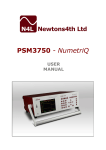
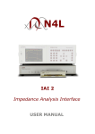
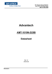
The QuanteQ has two processors:
a DSP (digital signal processor) for data analysis
a CPU (central processing unit) for control and display
At the heart of the system is an FPGA (field programmable
gate array) that interfaces the various elements.
OUT
CH1
CH2
CPU
FPGA
DSP
1-1
QuanteQ user manual
This general purpose structure provides a versatile
hardware platform that can be configured by firmware to
provide a variety of test functions, including:
signal generator
pulse generator
two channel true rms voltmeter
phase angle voltmeter (vector voltmeter)
two channel digital storage oscilloscope
frequency response analyser (gain/phase analyser)
phase meter
phase sensitive detector
dual frequency generator
harmonic analyser
two channel dual frequency selective level meter
transformer analyser
With additional external interface boxes, such as current
shunts, other functions are possible:
true rms current meter
LCR meter
power meter
transformer analyser
QuanteQ is configured to perform the required test
function by simple user menus, or can be controlled
remotely via a serial interface.
The programmable nature of the instrument means that
new functions can be added as they become available, or
existing functions can be enhanced, by simple firmware
download.
1-2
QuanteQ user manual
1.1
Generator output
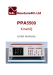
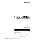
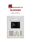
The generator consists of a DAC whose input is derived
from a table held in RAM. The appropriate pattern is
loaded into the RAM (sinewave, sawtooth, dual frequency
etc.) by the DSP, then the RAM address is stepped at a
rate given by the selected frequency. The output of the
DAC is attenuated, has any offset added, is filtered and is
buffered by a high speed, high current buffer.
The DAC is clocked at 23.04MHz.
The DAC resolution is 16 bit.
The RAM depth is 32k words x 16 bit.
The maximum output level is ±10V peak.
The maximum output current is ±200mA peak.
The 0V of the output is earthed.
There is a 50Ω output impedance.
There is a separate analogue white noise generator that
can be selected instead of the DAC output. The rest of the
attenuation, offset, filtering, and buffering circuitry is the
same.
noise
attenuate
offset
filter
RAM
50Ω
DAC
output
buffer
1-3
QuanteQ user manual
1.2
Voltage inputs
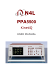
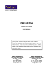
Each input consists of a high impedance buffer followed by
switch to select ac or ac+dc coupling, then a series of gain
stages leading to an A/D converter. Selection of the input
gain and the sampling of the A/D converter are under the
control of the DSP by communication across an isolation
barrier. There is an autozero switch at the front end for dc
accuracy.
Both input channels have their own isolated power supplies
and are fully floating from earth and from each other. The
isolation of the input channels with high CMRR allows
measurements to be made relative to any potential within
500V from earth. For example, the small voltage across a
current sense resistor can be measured, as the much
higher supply voltage will be rejected.
One consequence of the isolation is that each input must
have its signal 0V connected (unlike most oscilloscopes
which force the inputs to be earth referenced).
The
The
The
The
The
maximum input is ±500V peak.
full scale of the lowest range is ±10mV peak.
input frequency range is dc to 2.4MHz.
A/D converter resolution is 14 bit.
A/D sample rate is variable to 0.8M samples/s.
A/D
ac
dc coupled
input buffer
1-4
variable
gain
isolation
interface
QuanteQ user manual
2
Getting started
The QuanteQ is supplied ready to use – it comes complete
with an appropriate power lead and a set of test leads. It
is supplied calibrated and does not require anything to be
done by the user before it can be put into service.
2.1
Unpacking
Inside the carton there should be the following items:
one QuanteQ unit
one appropriate mains lead
two high voltage safety probes
one BNC output lead with clips
one null modem cable to connect to a computer
this manual
Having verified that the entire above list of contents is
present, it would be wise to verify that your QuanteQ
operates correctly and has not been damaged in transit.
First verify that the voltage rating on the rear of the
QuanteQ is appropriate for the supply, then connect the
mains cord to the inlet on the rear panel of the QuanteQ
and the supply outlet.
Switch on the QuanteQ. The display should illuminate with
the company logo and the firmware version for a few
seconds while it performs some initial tests. It should then
default to the RMS voltmeter display. Note that the switch
on message can be personalised – see the User Data
section under System Options.
Note that if there are no leads connected, the rms display
should read zero. If any test leads are connected then
2-1
QuanteQ user manual
because of the high impedance of the inputs, the rms
display may read some random values due to noise pick
up. If the unit does display any values with no leads
connected, give the unit two minutes to warm up then
press ZERO.
Connect the output lead to the output connector of the
Veqtor and the input probes to the two input connectors.
Connect the output to both of the inputs by connecting the
black clip on the output lead to the 0V clip on each of the
input probes, and the red clip of the output lead to the
input probes. Note that this is easiest to do by connecting
across a resistor (any value above 1k).
Press the OUT key to invoke the output menu, then press
the UP key to select the output on/off control then the
RIGHT key to turn on the output.
Exit the menu by pressing the HOME button twice.
The display should now indicate an rms value of ~1.4V on
both channels, each of which should indicate the 3V range.
Press the FUNC key to select the gain phase analyser
function and check that the gain reads 0dB ±0.05dB, and
that the phase reads ≤ 0.01°.
In the event of any problem with this procedure, please
contact customer services at Newtons4th Ltd. or your local
authorised
representative:
contact
addresses
and
telephone numbers are given in the appendix.
2-2
QuanteQ user manual
2.2
Keyboard and controls
The keyboard is divided into 3 blocks of keys:
display control (6 top keys)
menu control (middle 9 keys)
setup keys (lower 12 keys)
In normal operation, the menu control (cursor) keys give
one-touch adjustment of various parameters, such as
generator amplitude, without having to access the menu
system.
The display control and setup keys also have a secondary
function for numeric entry in the menu system.
RMS
SCOPE
FUNC
BACK
DISP
ZOOM+
UP
LEFT
DELETE
ZOOM-
NEXT
HOME
RIGHT
DOWN
ENTER
SYSTEM
MODE
OUT
CH1
CH2
SETUP
PRINT
ALARM
PROG
START
ZERO
STEP
2-3
QuanteQ user manual
Primary key action (normal operation)
RMS
Selects RMS voltmeter function (or loads
program).
SCOPE
Selects oscilloscope function (or loads program).
FUNC
Selects chosen test function (or loads program).
Note: the above keys allow one-touch switching between
RMS, oscilloscope, or any other function, or stored programs.
DISP
Selects display mode or long press initiates
HOLD.
ZOOM+
Increase zoom level (where appropriate).
ZOOMDecrease zoom level (where appropriate).
BACK
Action depends on measurement function.
DELETE
Action depends on measurement function.
NEXT
Action depends on measurement function.
ENTER
Action depends on measurement function.
UP
Step up generator amplitude.
DOWN
Step down generator amplitude.
RIGHT
Step up generator frequency.
LEFT
Step down generator frequency.
Note: the step size for the above can be set via the menus.
HOME
Retrigger
SYSTEM
MODE
OUT
CH1
CH2
SETUP
PRINT
ALARM
PROG
START
ZERO
STEP
2-4
System options menu.
Main operating mode menu.
Output control menu.
Input channel 1 control menu.
Input channel 2 control menu.
Function setup menu.
Printout control menu.
Alarm control menu.
Program save and recall menu.
Start sweep or integration (depends function).
Perform offset compensation.
Step control menu.
QuanteQ user manual
Secondary key action (menu mode)
RMS
SCOPE
FUNC
DISP
ZOOM+
ZOOM-
‘G’ multiplier (x 109), or ‘A’ for text.
‘M’ multiplier (x 106), or ‘E’ for text.
‘k’ multiplier (x 103), or ‘I’ for text.
‘m’ multiplier (x 10-3), or ‘O’ for text.
‘µ’ multiplier (x 10-6), or ‘U’ for text.
‘n’ multiplier (x 10-9), or ‘space’ for text.
NEXT
Step to next menu, or next character for text.
BACK
Back to previous menu or character for text.
UP
Cursor up, or upper case for text.
DOWN
Cursor down, or lower case for text.
RIGHT
Step forward in a list or in data entry.
LEFT
Step backward in a list or in data entry.
DELETE
Delete previous character in data entry.
ENTER
Enter numerical value or text.
HOME
Return to start of menu, or exit if at the start.
Note: to exit any menu press HOME twice.
SYSTEM
MODE
OUT
CH1
CH2
SETUP
PRINT
ALARM
PROG
START
ZERO
STEP
0 in a data entry, or jump to item 0 in a list.
1 in a data entry, or jump to item 1 in a list.
2 in a data entry, or jump to item 2 in a list.
3 in a data entry, or jump to item 3 in a list.
4 in a data entry, or jump to item 4 in a list.
Insert minus sign in a data entry (if valid).
5 in a data entry, or jump to item 5 in a list.
6 in a data entry, or jump to item 6 in a list.
7 in a data entry, or jump to item 7 in a list.
8 in a data entry, or jump to item 8 in a list.
9 in a data entry, or jump to item 9 in a list.
Insert decimal point in a data entry (if valid).
Toggle autoranging in channel menu.
Set alarm limits in alarm menu.
2-5
QuanteQ user manual
2.3
Basic operation
Once the unit has powered on and is displaying the default
RMS voltmeter screen, the simplest way to configure the
instrument is to start at the ‘operating mode’ screen and
step through the menus using the NEXT key. The
instrument will present a sequence of menus then exit to
the normal operating screen.
Press
Press
Press
Press
Press
Press
Press
MODE
NEXT
NEXT
NEXT
NEXT
NEXT
NEXT
select the main function required.
select the output conditions required.
change the channel 1 setup if needed.
change the channel 2 setup if needed.
select the options for the main function.
further options for the main function if any.
exit menu sequence.
For more detail about the menu system refer to the next
chapter.
For example, to use the gain/phase analyser on a circuit
under test, connect the output of the QuanteQ to the input
of the circuitry, connect channel 1 also to the input of the
circuitry, and connect channel 2 to the output of the
circuitry.
Press MODE and select gain phase analyser.
Press NEXT, select the amplitude and turn the output on.
Press NEXT, NEXT, NEXT, select the number of steps, the
start frequency and stop frequency.
Press NEXT, NEXT.
The instrument will now display the gain and phase of the
transfer function of the circuit under test at the spot
frequency specified by the output control menu.
Press LEFT or RIGHT to adjust the frequency, Press UP or
DOWN to adjust the amplitude. (In order to change the
2-6
QuanteQ user manual
size of the steps when using the cursor keys in normal
operation, use the STEP menu).
Press START and QuanteQ will start a frequency sweep
over the specified range.
Pressing DISP selects the display option:
spot frequency result
table (step through with NEXT and BACK)
gain graph
phase graph
gain + phase graph simultaneously
Pressing PRINT allows two lines of print title to be entered
and prints the selected display plus the table of results and
the setup information.
Press HOME to revert to the real time display at a spot
frequency.
There are three ways to change the measurement
function:
MODE menu
RMS, SCOPE, FUNC keys
FUNC key + one of the setup keys within 1.5s
2-7
QuanteQ user manual
3
Using the menus
QuanteQ is a very versatile instrument with many
configurable parameters. These parameters are accessed
from the front panel via a sequence of menus.
Each of the main menus may be accessed directly from a
specific key (e.g. output menu using OUT key, function
setup menu using SETUP key) or may be invoked in a
logical sequence using the NEXT key.
The main menu sequence is:
MODE menu
OUTPUT menu
CH1 menu
CH2 menu
SETUP menu(s)
In order to configure QuanteQ, start at the MODE menu to
select the main function then keep pressing the NEXT key
checking each menu and modifying any parameters as
required. When all relevant menus have been displayed,
QuanteQ reverts back to normal operation in the selected
mode.
Note that the BACK key steps through the menus in the
reverse sequence.
Additionally there are some other menus that are not
linked by the NEXT key:
SYSTEM menu (use dedicated SYSTEM key)
STEP menu (use dedicated STEP key)
ALARM menu (use dedicated ALARM key)
PROGRAM menu (use dedicated PROG key)
3-1
QuanteQ user manual
Each menu starts with the currently set parameters visible
but no cursor. In this condition, pressing the menu key
again or the HOME key aborts the menu operation and
reverts back to normal operation.
To select any parameter, press the UP or DOWN key and a
flashing box will move around the menu selecting each
parameter. In this condition the keys take on their
secondary function such as numbers 0-9, multipliers n-G
etc.
Pressing the HOME key first time reverts to the opening
state where the parameters are displayed but the cursor is
hidden. Pressing the HOME key at this point exits the
menu sequence and reverts back to normal operation.
To abort the menu sequence, press the HOME key
twice.
There are three types of data entry:
selection from a list
numeric
text
3-2
QuanteQ user manual
3.1
Selection from a list
This data type is used where there are only specific options
available such as the output may be ‘on’ or ‘off’, the graph
drawing algorithm may use ‘dots’ or ‘lines’.
When the flashing cursor is highlighting the parameter, the
RIGHT key steps forward through the list, and the LEFT
key steps backwards through the list. The number keys 09 step directly to that point in the list, which provides a
quick way to jump through long lists. There is no need to
press the ENTER key with this data type
For example, if the waveform selection list comprises the
options:
sinewave
(item 0)
triangle wave
(item 1)
square wave
(item 2)
leading sawtooth
(item 3)
trailing sawtooth
(item 4)
and the presently selected option is sinewave, there are 3
ways to select leading sawtooth:
press RIGHT three times
press LEFT twice
press number 3
3-3
QuanteQ user manual
3.2
Numeric data entry
Parameters such as frequency and offset are entered as
real numbers; frequency is an example of an unsigned
parameter, offset is an example of a signed parameter.
Real numbers are entered using the number keys,
multiplier keys, decimal point key, or +/- key (if signed
value is permitted). When the character string has been
entered, pressing the ENTER key sets the parameter to the
new value. Until the ENTER key is pressed, pressing the
HOME key aborts the data entry and restores the original
number.
If a data value is entered that is beyond the valid limits for
that parameter then a warning is issued and the
parameter set as close to the requested value as possible.
For example, the maximum amplitude of the QuanteQ
generator is 10V peak; if a value of 15V is entered, a
warning will be given and the amplitude set to the
maximum of 10V.
When the parameter is first selected there is no character
cursor visible – in this condition, a new number may be
entered directly and will overwrite the existing number.
To edit a data value rather than overwrite it, press the
RIGHT key and a cursor will appear. New characters are
inserted at the cursor position as the keys are pressed, or
the character before the cursor position can be deleted
with the DELETE key.
Data values are always shown in engineering notation to 5
digits (1.0000-999.99 and a multiplier).
3-4
QuanteQ user manual
3.3
Text entry
There are occasions where it is useful to enter a text
string; for example, any printout may have two lines of
text as a title.
Text is entered by selecting one of 6 starting characters
using the display control keys on the top row of the
keyboard, then stepping forwards or backwards through
the alphabet with the NEXT and BACK keys.
The starting letters from left to right are A, E, I, O, U, or
space.
Numbers can also be inserted using the number keys.
The NEXT and BACK keys step forward and backward
using the ASCII character definitions – other printable
characters such as # or ! can be obtained by stepping on
from the space. The available character set is given in the
Appendix.
When entering alphabetic characters, the UP and DOWN
keys select upper and lower case respectively for the
character preceding the cursor and the next characters to
be entered.
The editing keys, RIGHT, LEFT, DELETE and ENTER
operate in the same way as for numeric entry.
3-5
QuanteQ user manual
4
4.1
Special functions
Display zoom
QuanteQ normally displays many results on the screen in a
small font size. Where only one or two results are of
interest, the zoom function allows those results to be
displayed in a larger font size.
There are two zoom levels:
Up to four results each approx. double normal size
A single result approx. four times normal size
To invoke the zoom function from any screen with numeric
results, press the ZOOM+ key.
If no zoom parameters have already been selected, a
flashing box will surround the first result. The flashing box
is moved around the available results using the cursor
keys, UP, DOWN, LEFT and RIGHT. Pressing the ENTER
key selects the result for zoom and the box ceases to
flash. Further results (up to four in total) can then be
selected using the cursor keys in the same way – a solid
box remains around the already selected item, and a new
flashing box appears.
Having selected the desired results, pressing the ZOOM+
key invokes the first zoom level, pressing it again selects
the higher level. Pressing ZOOM-, steps back down one
level each time.
Next time that ZOOM+ is pressed from the normal screen,
the screen shows the previously selected parameters.
These can be accepted by pressing the ZOOM+ key again,
or may be cleared using the DELETE key.
4-1
QuanteQ user manual
4.2
Program store and recall
There are 100 non-volatile program locations where the
settings for the entire instrument can be saved for recall at
a later date. Each of the 100 locations has an associated
name of up to 20 characters that can be entered by the
user to aid identification.
Program number 1 (if not empty) is loaded when the
instrument is powered on, so that QuanteQ can be set to a
user defined state whenever it is switched on. This is
particularly useful to set system options such as phase
convention or printer type. If no settings have been stored
in program 1 then the factory default settings are loaded
(program number 0).
The instrument can be restored to the factory default
settings at any time by recalling program number 0.
The program menu is accessed using the PROG key. The
program location can be selected either by stepping
through the program locations in turn to see the name, or
by entering the program number directly. To print out a
directory of stored programs, press PRINT while in the
program menu.
When storing a configuration in a program, there will be a
slight pause (of about 1 second) if the program has
previously been written or deleted, or the process will be
very quick if the location has not been used.
Each of the ‘one-touch’ keys – RMS, SCOPE, and FUNC –
may optionally be set to load a specified program instead.
When supervisor mode is disabled (see system options),
programs can only be recalled, not stored nor deleted, to
avoid accidental modification.
4-2
QuanteQ user manual
4.3
Zero compensation
There are 3 levels of zero compensation:
Trim out the dc offset in the input amplifier chain.
Measure any remaining offset and compensate.
Measure parasitic external values and compensate.
The trim of the dc offset in the input amplifier chain is reapplied every time that the measurement function is
changed, or can be manually invoked with the ZERO key,
or over the RS232 with the REZERO command.
The measurement of the remaining offset also happens
when the offset is trimmed but is also repeated at regular
intervals when using a measurement function that requires
dc accuracy (such as the rms voltmeter). This is to
compensate for any thermal drift in the amplifier chain.
This repeated autozero function can be disabled via the
SYSTEM OPTIONS menu.
The compensation for parasitic external values (for
example to compensate for the capacitance of the test
leads when measuring capacitance) is invoked manually by
the ZERO key. Refer to each function section for the
function specific operations.
Any compensation values are stored along with the
instrument configuration when a program is stored.
To
restore
operation
without
function
compensation press ZERO then DELETE.
specific
4-3
QuanteQ user manual
4.4
Alarm function
QuanteQ has an audible alarm that can be used in a
variety of ways:
sound the alarm if the value exceeds a threshold
sound the alarm if the value is below a threshold
sound the alarm if the value is outside a window
sound the alarm if the value is inside a window
vary the alarm linearly between thresholds
The value to which the alarm is applied can be any of the
measurements selected for zoom.
To program an alarm, first select the functions for the
zoom; up to four measurements can be selected for the
display, the alarm is applied to any of them; then press
ALARM to invoke the alarm menu:
select which of the zoom functions is to be used
select the type of alarm
set the upper limit (if appropriate)
set the lower limit (if appropriate)
select whether the alarm is to be latched
If the alarm latch is selected then the alarm will continue
to sound even if the value returns to within the normal
boundaries. To clear the alarm, press HOME.
The linear alarm option allows tests to be carried out even
if it is not possible to see the display. Pressing STEP in the
alarm menu sets the upper and lower threshold to 4/3 and
1/3 of the measured value respectively. The repetition rate
of the sounder then varies linearly as the value changes
between these thresholds.
4-4
QuanteQ user manual
4.5
Data hold
The data on the display can be held at any time by
pressing and holding down the DISP key for ½ second.
When HOLD is activated a warning message is briefly
displayed and the word HOLD appears in the top right
hand corner of the display. The held data is that present
when the DISP key was first recognised.
While HOLD is active, the DISP key operates as normal so
that other values may be viewed while the data is not
changing (eg. rms and watts in power meter mode).
Press the HOME key or START key to release HOLD; in this
case, HOME and START do not have their normal
functions. Changing mode also releases hold.
When HOLD has been activated, the DSP continues to
sample, compute and filter the results but the data is
ignored by the CPU. When HOLD is released the display is
updated with the next available value from the DSP.
4-5
QuanteQ user manual
5
Using remote control
QuanteQ is fitted with an RS232 serial communications
port as standard, and may have an IEEE488 (GPIB)
interface fitted as an option. The two interfaces use the
same ASCII protocol with the exception of the end of line
terminators:
RS232
IEEE488
Rx expects
carriage return
(line feed ignored)
carriage return or
EOI
Tx sends
carriage return
and line feed
carriage return
with EOI
All the functions of the QuanteQ can be programmed via
either interface, and results read back. When the IEEE488
interface is set to ‘remote’ the RS232 port is ignored.
The commands are not case sensitive and white space
characters are ignored (e.g. tabs and spaces). Replies
from QuanteQ are always upper case, delimited by
commas, without spaces.
Only the first six characters of any command are important
– any further characters will be ignored. For example, the
command to set the timebase for the oscilloscope function
is TIMEBA but the full word TIMEBASE may be sent as the
redundant SE at the end will be ignored.
Fields within a command are delimited by comma, multiple
commands can be sent on one line delimited with a semicolon.
Mandatory commands specified in the IEEE488.2 protocol
have been implemented, (e.g. *IDN?, *RST) and all
commands that expect a reply are terminated with a
question mark.
5-1
QuanteQ user manual
QuanteQ maintains an error status byte consistent with
the requirements of the IEEE488.2 protocol (called the
standard event status register) that can be read by the
mandatory command *ESR? (see section 5.1).
QuanteQ also maintains a status byte consistent with the
requirements of the IEEE488.2 protocol, that can be read
either with the IEEE488 serial poll function or by the
mandatory command *STB? over RS232 or IEEE (see
section 5.2).
The IEEE address defaults to 23 and can be changed via
the SYSTEM menu.
The keyboard is disabled when the instrument is set to
“remote” using the IEEE. Press HOME to return to “local”
operation.
RS232 data format is: start bit, 8 data bits (no parity), 1
stop bit. Flow control is RTS/CTS (see section 5.2), baud
rate is selectable via the SYSTEM menu.
A summary of the available commands is given in the
Appendix. Details of each command are given in the
“QuanteQ communication manual”.
Commands are executed in sequence except for two
special characters that are immediately obeyed:
Control T (20) – reset interface (device clear)
Control U (21) – warm restart
5-2
QuanteQ user manual
5.1
Standard event status register
PON
CME
EXE
DDE
QYE
OPC
bit 0 OPC
(operation complete)
cleared by most commands
set when data available or sweep complete
bit 2 QYE (unterminated query error)
set if no message ready when data read
bit 3 DDE (device dependent error)
set when the instrument has an error
bit 4 EXE (execution error)
set when the command cannot be executed
bit 5 CME (command interpretation error)
set when a command has not been recognised
bit 7 PON (power on event)
set when power first applied or unit has reset
The bits in the standard event status register except for
OPC are set by the relevant event and cleared by specific
command (*ESR?, *CLS, *RST). OPC is also cleared by
most commands that change any part of the configuration
of the instrument (such as MODE or START).
5-3
QuanteQ user manual
5.2
Serial Poll status byte
ESB
bit 0 RDV
bit 1 SDV
bit 2 FDV
bit 4 MAV
bit 5 ESB
5-4
MAV
FDV
SDV
RDV
(result data available)
set when results are available to be read as
enabled by DAVER
(sweep data available)
set when sweep results are available to be
read as enabled by DAVER
(fast data available (streaming))
set when data streaming results are available
to be read as enabled by DAVER
(message available)
set when a message reply is waiting to be read
(standard event summary bit)
set if any bit in the standard event status
register is set as well as the corresponding bit
in the standard event status enable register
(set by *ESE).
QuanteQ user manual
5.3
RS232 connections
The RS232 port on QuanteQ uses the same pinout as a
standard 9 pin serial port on a PC or laptop (9-pin male ‘D’
type).
Pin
Function
Direction
1
2
3
4
5
6
7
8
9
DCD
RX data
TX data
DTR
GND
DSR
RTS
CTS
RI
in (+ weak pull up)
in
out
out
not used
out
in
not used
QuanteQ will only transmit when CTS (pin 8) is asserted,
and can only receive if DCD (pin 1) is asserted. QuanteQ
constantly asserts (+12V) DTR (pin 4) so this pin can be
connected to any unwanted modem control inputs to force
operation without handshaking. QuanteQ has a weak pull
up on pin 1 as many null modem cables leave it open
circuit. In electrically noisy environments, this pin should
be driven or connected to pin 4.
To connect QuanteQ to a PC, use a 9 pin female to 9 pin
female null modem cable:
1&6
2
3
4
5
7
8
-
4
3
2
1&6
5
8
7
5-5
QuanteQ user manual
5.4
Data streaming
The phase meter, phase angle voltmeter and power meter
modes have the option of high speed data streaming. In
this operation, the window width for the measurement
may be specified from 660us to 100ms and the data for
each measurement window is transmitted over the
communications in a continuous stream. The window is
adjusted to synchronise to the measured frequency.
QuanteQ buffers the data and transmits at the fastest rate
that is possible. The buffer depth is over 8000 data values
so more than 5 seconds of data can be captured at the
fastest rate of 1500 readings per second even if the data is
not read at all. If the window size is such that the data can
be read out in real time then data streaming can continue
indefinitely.
Once the data streaming window has been setup, the
display periodically shows the measured value. Once
streaming has been started, the display is blanked to
minimise processing overheads. Streaming can be stopped
either immediately (ABORT) or may be stopped but
remaining data continues to be transmitted until the buffer
is empty (STOP).
STREAM,ENABLE,0.01
START
read data
STOP
continue to read stored data
5-6
QuanteQ user manual
6
Using the printer
The QuanteQ has a parallel output port for directly driving
an external printer.
The printout consists of:
Optional 1 or 2 line title
Header with the user data and serial number
Setup information
Table of data if available (such as frequency sweep)
Graph if available
Where a sweep has been performed (such as when using
the gain/phase analyser) or when a waveform is on the
display then one or more graphs can be printed with a
table of results; otherwise the available data from the realtime analysis is printed. The sweep printout may be
selected as:
table and graph
table only
graph only
A sequential number can be printed out as part of the title
line by entering the code ## (start with space and press
NEXT). This helps to keep a series of printouts in the
correct sequence.
The data to be printed and the associated instrument
settings are captured internally to a printer buffer when
the print key is pressed so that the instrument settings can
be changed once printing has started.
The printer output may be in the format for an HP inkjet
such as Deskjet 600 (also some laser printers), an Epson
inkjet that accepts the ESC /P2 command set (such as the
Stylus range), or Canon bubblejet such as the portable
BJC-80. As printers often have selectable emulation
modes, it may be necessary to check that the printer has
6-1
QuanteQ user manual
the correct setting (the BJC-80 often defaults to an
incompatible Epson format).
The timeout on each printed character can be adjusted via
the SYSTEM menu. This may be necessary if using a very
slow printer.
If no printer is connected to the printer port then the 8
data output lines and the 5 control input lines may be used
as general purpose logic level I/O lines for controlling or
monitoring external equipment.
Input lines:
7
6
5
4
ACK
6.1
3
BUSY
2
END
1
0
SLI
ERR
Printer port connection
The QuanteQ printer port uses the same pinout and
connector (25-pin female ‘D’ type) as is used on a PC. A
standard PC to Centronics printer cable is required.
6-2
QuanteQ user manual
7
System options
Press SYSTEM to access the system options.
There are two levels of brightness for the display: bright or
dim. Dim can be selected for low ambient light conditions
where the very high contrast of the display may be
uncomfortable; or may be automatically selected if there
has been no key presses for 20 minutes.
The graphs on the display and printout may be made up of
single points or lines.
Each key press is normally accompanied by an audible
‘beep’ as well as the tactile ‘click’. The ‘beep’ can be
disabled for quiet environments if the feel of the key is
sufficient feedback
Measurements of phase can be expressed in one of three
conventional formats:
-180° to +180° (commonly used in circuit analysis)
0° to -360° (commonly used in power applications)
0° to +360°
The measurement is exactly the same it is only the way
that it is expressed that changes.
Regular autozero measurements can be suppressed.
Press NEXT to access the second system menu.
‘Program step’ allows a sequence of user configurations to
be stepped through using NEXT and BACK keys. Store the
desired configurations in the program locations and when
‘program step’ is enabled, the configurations may be
selected by pressing NEXT and BACK. Any empty program
stores are ignored.
Low value blanking can be disabled.
7-1
QuanteQ user manual
Some functions, such as LCR meter and transformer
analyser, can automatically change the test conditions
(frequency and amplitude) to suit the component under
test. Manually changing the conditions disables the
automatic function.
The shunt value is usually selected automatically when
changing function to one that needs a current input such
as power meter or LCR meter. If the ‘automatic shunt’
option is disabled then the shunt value will not be
changed.
Any measurements that are expressed in length (eg.
LVDT) can be displayed in metres or inches.
Press NEXT to access the third system menu.
The printer timeout can be adjusted for slower printers.
The RS232 Baud rate can be selected from 1200 to 19200.
Emulation can be enabled or disabled.
If the IEEE card is fitted, the address can be set from 130.
To save these system settings as default, store the setup
in program 1 so that they are reloaded on power on.
Pressing NEXT from the third SYSTEM OPTIONS menu
selects the USER DATA screen.
Pressing BACK from the first SYSTEM OPTIONS menu
displays the serial number and release versions.
7-2
QuanteQ user manual
7.1
User data
QuanteQ can be personalised by entering up to 3 lines of
user data as text (see section on text entry).
The first line is displayed every time that the instrument is
switched on, the other two lines, if entered, are also
printed out in the header to identify the instrument.
Typical arrangement of the user data would be:
line 1 company name
line 2 department or individual name
line 3 unique identifying number (eg. asset number)
Any user data may be entered as required, as the lines are
treated purely as text and are not interpreted by QuanteQ
at all.
After changing the user data, execute ‘store’ to save the
data in non-volatile memory.
The entered text may also be read over the RS232 to
identify the instrument (see USER?).
For use in a production environment, QuanteQ supports
two modes of operation, supervisor and user. When
supervisor mode is disabled, the stored programs can only
be recalled, not changed. QuanteQ saves the mode of
operation with the user data so that it may be configured
to power up in either mode as required.
7-3
QuanteQ user manual
8
Mode options
The main measurement function for the instrument may
be manually selected in one of three ways:
‘one-touch’ keys, RMS, SCOPE or FUNC,
FUNC key + a setup key within 1.5s,
the MODE menu.
The setup keys have the following effect when pressed
within 1.5s of the FUNC key:
SYSTEM power meter
OUT
gain/phase analyser
CH1
harmonic analyser
CH2
phase meter
PRINT
LCR meter
ALARM
vector voltmeter
PROG
transformer analyser
START
selective level meter
Once the mode is set, the FUNC key will restore the
previously selected mode. For example, if the frequency
meter is selected it is possible to switch to rms voltmeter,
scope, and back to frequency meter using the ‘one-touch’
keys without going back to the MODE menu.
The output mode may be one of the available generators:
disabled
sin/squ/tri
dc only
pulse
white noise
dual frequency
Each input channel may be selected to be:
disabled
voltage
external shunt
8-1
QuanteQ user manual
If the external shunt option is selected, the data is scaled
by the shunt value (entered under the relevant channel
menu) and the units are displayed in Amps. Any resistor
can be used as a shunt, or precision low inductance
current shunts are available as accessories. Current
transformers can be used if fitted with an appropriate
burden resistor.
Note that the external shunt input polarity is
reversed compared to that of the voltage input: ie
the outer screen of the input connector is positive
and the inner contact is negative. This is so that the
capacitance to ground of the input channel 0V is driven
with the lower source impedance in order to minimise
errors at high frequency.
Note that some modes force the input channels to be
voltage or current automatically, eg. the power meter
defaults to channel 1 as voltage and channel 2 as current.
This automatic selection can be overridden if required.
Some control parameters that relate to the operation of
the instrument as a whole rather than a specific
measurement are common across all the relevant
measurement functions. For example, when synchronising
to the input frequency, there is a low frequency option that
extends the frequency measurement down to 20mHz. If
this parameter is set in any measurement function (eg.
vector voltmeter) it applies also to any other function that
uses it (eg. power meter).
The window over which the measurements are computed
is adjusted to give an integral number of cycles of the
input waveform. The results from each window are passed
through a digital filter equivalent to a first order RC low
pass filter.
8-2
QuanteQ user manual
There are three speed options - slow, medium and fast that adjust the nominal size of the window, and therefore
the update rate and the time constant of the filter. Greater
stability is obtained at the slower speed at the expense of
a slower update rate.
Note that at low frequencies, the window is extended to
cover a complete cycle of the input waveform even if this
is a longer period than the nominal update rate.
There are two time constants for the filter, normal or slow,
or the filter can be deselected. The filter applies an auto
reset function to give a fast dynamic response to a change
of measurement – this function can be deselected and the
filter forced to operate with a fixed time constant for use
with noisy signals.
The nominal values are:
speed
update
rate
normal
time
constant
slow time
constant
fast
medium
slow
1/20s
1/3s
2.5s
0.2s
1.5s
12s
0.8s
6s
48s
These common parameters can be set as part of the
function SETUP menu where appropriate.
8-3
QuanteQ user manual
9
Output control
The output for the signal generator, pulse generator, and
dual frequency generator are digitally synthesised at an
update rate of 23.04Msamples/s. This gives very good
sinewave waveform, even at 2.4MHz, while preserving
very accurate frequency control. Output filtering removes
the stepped effect of the sampling.
The white noise generator, however, is a separate analog
circuit to give true, non-repetitive noise.
The output for the signal generator, noise generator, and
dual frequency generator pass through a logarithmic
attenuator equivalent to 17 bits so that very fine
amplitude increments are possible at low signal levels.
The pulse generator bypasses this attenuator to improve
the rising and falling edges that are limited only by the
output filtering. The amplitude of the pulse is set directly
by the output DAC. The rising and falling edges can be set
to be slower.
An offset may be added to any output to bias the signal or
to null out any dc present.
The output parameters of each generator are stored
separately so that changing the output amplitude of the
pulse generator does not change the output amplitude
configured for the signal generator when that is next
selected.
The LEFT and RIGHT keys adjust the frequency of the
generator by a fixed increment stored via the STEP menu;
the UP and DOWN keys adjust the amplitude.
The RS232 commands are common for each generator and
are applied to whichever generator has been selected.
9-1
QuanteQ user manual
The signal generator has a trim function that controls the
measured level to a specified accuracy. This is particularly
useful to maintain a consistent excitation level during a
frequency sweep (amplitude compression). At each
measurement point, the measured level is checked against
the specified level and tolerance; if an adjustment is
needed the data is discarded and a new measurement
made at the new output level. The user is alerted to the
adjustment by an audible beep.
Both dc and ac components can use independent control
values.
Note that as the trim functions compute a new generator
level by scaling:
new level = present x specified / measured
the trim function can be used even if there are amplifiers
or attenuators between the generator output and the input
channel but cannot be used to trim out dc offsets to zero.
The dual frequency generator can be used in two modes,
FSK or harmonics. In FSK mode, the waveform consists of
half one frequency then half the second frequency; in
harmonic mode, both frequency components are present
all the time.
Note that the frequency specified for the dual frequency
generator is the repetition frequency of the composite
waveform. It is only the same as the fundamental
frequency in harmonic mode if one of the components is
specified as 1 cycle.
9-2
QuanteQ user manual
Generator specifications
General
frequency ±0.1%
accuracy
amplitude ±2.5% (to 100kHz)
output impedance 50Ω ±10%
±10V to ±10mV peak
output voltage
±10V peak maximum
offset
waveforms
frequency
Signal generator
sine, triangle, square, sawtooth, dc
only
100uHz to 2.4MHz (sine)
20mHz to 1MHz (other)
frequency
pulse width
resolution
rise and fall time
Pulse generator
100uHz to 1MHz
200ns to 10s
50ns
50ns (5V) to 1s
output voltage
Noise generator
~10mV to ~0.5V rms
repetition
frequency
components
number of cycles
type
Dual frequency generator
100uHz to 2.4MHz / n
2
1 to 50
FSK or harmonics
9-3
QuanteQ user manual
10 Input channels
The two input channels consist are electrically isolated
from each other and from earth, and are controlled
independently but sampled synchronously.
The input ranges have nominal full scale values set with a
ratio of 1:√10 from 10mV to 1000V (although the input is
rated at 500V maximum.). This gives the following ranges:
range
reference
nominal full scale
attenuator
1
2
3
4
5
6
7
8
9
10
11
10mV
30mV
100mV
300mV
1V
3V
10V
30V
100V
300V
500V
10mV
31.6mV
100mV
316mV
1V
3.16V
10V
31.6V
100V
316V
1000V (500V max)
low
low
low
low
low
low
low
high
high
high
high
Additionally, there are some special ranges, marked with
an asterisk that use different attenuator settings
range
reference
nominal full scale
attenuator
12
13
14
15
16
300mV*
1V*
3V*
10V*
30V*
316mV
1V
3.16V
10V
31.6V
high
high
high
high
low
The ranges may be selected manually, or by autoranging
(default). The start range for autoranging may be selected
if it is known that the signal will not be below a certain
level.
10-1
QuanteQ user manual
There is also an option to autorange ‘up only’ so that a test
may be carried out to find the highest range. Once the
highest range has been determined, the range can be set
to manual and the test carried out without losing any data
due to range changing. Pressing the HOME key (or sending
*TRG) restarts the autoranging from the selected
minimum range.
When in an input channel menu, the STEP key provides a
quick way to lock and unlock the range. When no flashing
box is visible in the input channel menu and autoranging is
selected, pressing the STEP key selects the range that the
instrument is currently using and sets the autoranging to
manual, thus locking the range and preventing further
autoranging. Pressing the STEP key again returns to full
autoranging from the bottom range.
For most measurement functions full autoranging is the
most suitable option but some applications, such as
viewing slow events on the oscilloscope, are more reliable
with manual ranging. Manual ranging (or up-only
autoranging) is essential for low frequency measurements.
For measuring signals that are biased on a dc level (such
as an amplifier operating on a single supply or the output
of a dc PSU), ac coupling can be used. This is particularly
useful for the oscilloscope option. AC+DC coupling is the
normal option and should be used where possible. There
are two ac coupling options that are selected according to
the size of the dc bias present:
< 10V dc
< 500V dc
Using the <10V option allows the instrument to autorange
from the 10mV range; the <500V option allows the
instrument to autorange from the 300mV range. When the
dc bias is greater than 10V it is essential that the <500Vdc
option is used for correct operation.
10-2
QuanteQ user manual
A scaling factor can be entered for each channel for use
with attenuators such as x10 oscilloscope probes. A
nominal value can be entered or the attenuation factor of
the probe can be measured and the precise value entered.
The measured voltage will be displayed after multiplication
by the scale factor.
Note that low voltage oscilloscope probes must not
be used where there are hazardous voltages – use
high voltage safety leads such as those supplied
with the instrument.
If the channel has been set for use with an external shunt
then the value of the shunt can be entered.
10-3
QuanteQ user manual
11 True RMS Voltmeter
The RMS voltmeter measures the total rms of the signal
present at the input terminals to the bandwidth of the
instrument (>2.4MHz). Care must be taken when
measuring low signal levels to minimise noise pick on the
input leads.
The RMS voltmeter measures the elementary values:
rms
dc
peak
surge
and derives the values: ac, dBm and crest factor.
The rms value of a periodic waveform, v(φ), is given by:
rms = √
[
2π
1/2π
∫
v2(φ) dφ
]
0
For a sampled signal, the formula becomes:
i = n-1
rms = √
[
1/n
∑ v [i] ]
2
i=0
where n is the number of samples for an integral number
of complete cycles of the input waveform.
These are fundamental definitions that are valid for all
waveshapes. For a pure sinewave, the formulae evaluate
to peak/√2, but this cannot be applied to other
waveshapes. QuanteQ computes the true rms value from
the fundamental definition for sampled data.
11-1
QuanteQ user manual
The dc present is given by:
dc = 1/2π
∫
2π
v(φ) dφ
0
For a sampled signal, the formula becomes:
i = n-1
dc = 1/n
∑ v[i]
i=0
where n is the number of samples for an integral number
of complete cycles of the input waveform.
Having computed the true rms and the dc component, the
ac component can be derived from:
rms2 = ac2 + dc2
=>
ac2 = rms2 – dc2
The ac component is also expressed in dB referred to 1mW
into 600Ω (dBm):
dBm = 20 log (Vac/Vref)
where Vref = √ (1mW x 600Ω)
or
20 log (Iac/Iref)
where Iref = √ (1mW / 600Ω)
The peak measurement is simply the value with the largest
magnitude. Positive and negative peaks are independently
filtered then the result with the largest magnitude is taken
as the peak value.
In order to measure surge conditions, the maximum
instantaneous peak value (unfiltered) is also recorded. It is
11-2
QuanteQ user manual
important
measuring
repeat the
maximum,
that QuanteQ does not autorange while
surge – either set the range to manual or
test with ranging set to up only. To reset the
press START.
Crest factor is derived from the peak and rms:
cf = peak / rms
The measurements are computed over rectangular
windows with no gaps. The processing power of the DSP
allows the measurements to be made in real time without
missing any samples. In this way, the measured rms is a
true value even if the signal is fluctuating. The only
occasion when data is missed is when an autozero
measurement is requested – this can be disabled in the
SYTEM OPTIONS menu.
The ZOOM function can be used to select any combination
of up to four parameters from the display.
DISP selects the measurement screen:
rms, dc, ac, dBm
rms, peak, crest factor, surge
11-3
QuanteQ user manual
RMS voltmeter specification
DVM
channels
2 isolated
display
5 digits
measurement
true rms, ac, dc, dBm, peak, cf, surge
coupling
ac or ac+dc
frequency
dc to >2.4MHz (ac+dc coupling)
ac coupling cut off ~1.5Hz (–3dB)
±500V peak
max input
±500V peak from earth
input ranges
500V, 300V, 100V, 30V, 10V, 3V, 1V,
300mV, 100mV, 30mV, 10mV
ranging
full auto, up only, or manual
input impedance
1M // 30pF (exc. leads)
accuracy (ac)
0.05% range + 0.05% reading +
0.3mV <1kHz
0.15% range + 0.15% reading +
0.3mV < 10kHz
0.5% range + 0.5% reading +
0.0025%/kHz + 0.3mV > 10kHz
accuracy (dc)
0.1% range + 0.1% reading + 0.5mV
CMRR (typical)
140dB @ 240V 50Hz
120dB @ 100V 1kHz
60dB @ 10V 1MHz
time constant
0.2s, 1.5s or 12s
Conditions:
23ºC +/- 5ºC ambient temperature
instrument allowed to warm up for ≥30 minutes
sinewave
slow speed, normal filtering
ac+dc coupling
autoranging or manual ranging ≥ 1/3 range
11-4
QuanteQ user manual
12 Low frequency storage oscilloscope
The QuanteQ provides a 2 channel storage oscilloscope
function with isolated inputs. The isolation of the inputs
makes it possible to view signals that are not earth
referenced (all normal oscilloscopes have their inputs tied
to earth). One consequence of the isolation, however, is
that it is essential to connect the 0V of both inputs. If both
inputs are connected to the same circuitry, it is not
sufficient to connect one 0V line and leave the other
floating.
The display for the oscilloscope is divided into 10 divisions
along the time axis with the selected timebase displayed in
units of time/division. The timebase may be set to any real
value between 20µs/div to 5s/div. Pressing BACK and
DELETE adjust the timebase by the factor stored via the
STEP menu (default 2). Thus the timebase may be
adjusted in fixed increments by a single key press, or may
be entered directly using the menu. For slow timebase
operation, (> 0.8s/div) the display operates in ‘roll’ mode
where the waveform scrolls across from left to right until
triggered.
The vertical scaling is shown as a full scale value, rather
than as a V/cm. This indicates the range that the
instrument is using for each channel.
The trigger level is set directly in Volts and does not
change if the range is changed, i.e. it is an absolute trigger
level and not relative to the range full scale. Pressing NEXT
and ENTER adjust the trigger level by a fixed increment
stored via the STEP menu (default 200mV).
The trigger may be set to rising edge or falling edge on
either channel 1 or channel 2.
12-1
QuanteQ user manual
The trigger level is shown as a small horizontal bar on the
extreme left-hand edge of the display against the
appropriate channel. If the trigger is set to a value above
or below the range of the input channel then a small carat
^ is shown at the top or inverted at the bottom of the
display as appropriate.
The trigger mode may be set to:
auto
(trigger if possible but do not wait for long)
normal
(wait indefinitely for trigger)
single shot
(wait for trigger then hold)
The single shot option is reset using the HOME key.
Pretrigger may be set to:
none
25%
50%
75%
Pretrigger is useful to see the conditions leading up to the
trigger event.
The display may be set to
Both channel 1 and channel 2
Channel 1 only
Channel 2 only
using the DISP key. When printing, the screen will be
printed with whichever channel(s) have been selected.
There are no ZOOM options with the oscilloscope mode.
Autoranging can be used with the oscilloscope functions
but it is more customary to fix the range manually. Manual
ranging is essential for rare events with a low mark space
ratio.
12-2
QuanteQ user manual
LF Oscilloscope specification
channels
timebase
roll mode
pretrigger
trigger
coupling
max input
input ranges
input impedance
ranging
Low frequency DSO
2 isolated
20us to 5s per division
timebase > 0.8s/div
none, 25%, 50%, or 75%
auto, normal, or single shot
ac or ac+dc
±500V peak
±500V peak from earth
500V, 300V, 100V, 30V, 10V, 3V, 1V,
300mV, 100mV, 30mV, 10mV
1M // 30pF (exc. leads)
full auto, up only, or manual
12-3
QuanteQ user manual
13 Frequency response analyser
QuanteQ measures the gain and phase of channel 2
relative to channel 1 using a discrete Fourier transform
(DFT) algorithm at the fundamental frequency.
The DFT technique can measure phase as well as
magnitude and is inherently good at rejecting noise – it is
much more reliable than measuring the rms at one point
relative to another point.
The circuit can be characterised by computing the gain and
phase at a number of points over a frequency range. This
gives results that show the transfer function of the circuit
as a graph on the display.
The DFT analysis yields two components – in-phase and
quadrature, or ‘a’ and ‘b’ values – from which the
magnitude and phase can be derived.
Considering
frequency:
the
components
at
the
fundamental
The fundamental in-phase and quadrature values of a
periodic waveform, v(φ), are given by:
a1 = 1/2π
b1 = 1/2π
∫
∫
2π
v(φ).cos(φ) dφ
0
2π
v(φ).sin(φ) dφ
0
13-1
QuanteQ user manual
For a sampled signal, the formulae become:
i = n-1
a1 = 1/n
∑ v[i].cos(2πci/n)
i=0
i = n-1
b1 = 1/n
∑ v[i].cos(2πci/n)
i=0
where n is the number of samples for an integral number
of complete cycles of the input waveform, and c is the
number of cycles.
Having computed the real and quadrature components, the
magnitude and phase of each channel can be derived:
mag = √ (a12 + b12)
θ = tan-1(b1/a1)
The relative gain and phase of the circuitry under test at
that particular frequency is derived from the real and
quadrature components by vector division:
vector gain = (a + jb) {ch2} / (a + jb) {ch1}
gain = magnitude (vector gain)
phase = tan-1(b/a (vector gain))
The gain is usually quoted in dB:
dB
13-2
= 20 log10(gain)
QuanteQ user manual
To look at differences in gain from a nominal value, an
offset gain can be applied either manually or by pressing
ZERO.
offset gain = measured dB – offset dB
The filtering is applied to the real and quadrature
components individually, rather than the derived
magnitude and phase values. This gives superior results as
any noise contribution to the components would have
random phase and therefore would be reduced by filtering.
QuanteQ can operate either in real time mode at a single
frequency where the gain and phase are filtered and
updated on the display; or it can sweep a range of
frequencies and present the results as a table or graphs of
gain and phase.
The frequency points to be measured are specified with
three parameters:
number of steps
start frequency
end frequency
QuanteQ computes a multiplying factor that it applies to
the start frequency for the specified number of steps. Note
that due to compound multiplication it is unlikely that the
end frequency will be exactly that programmed. The
frequency sweep is initiated by the START key, and when
completed the data can be viewed as a table or graphs or
printed out.
The window over which the measurements are computed
is adjusted to give an integral number of cycles of the
input waveform. In real time mode the results from each
window are passed through a digital filter equivalent to a
first order RC low pass filter; in sweep mode each result
comprises a single window without any filtering.
13-3
QuanteQ user manual
Very good results can be obtained in a reasonable time
using the medium speed setting (e.g. 50 points x ~1/3s ≅
17s); for the very best results, use the slow setting (50
points x ~2.5s ≅ 125s or 2 minutes, 5 seconds).
The top of the vertical axis for the graph is normally set to
be the highest measured value during the sweep. The
bottom of the vertical axis is normally either set to the
lowest measured value or the result of the highest value
less 20dB/decade of frequency. The vertical axis can be
fixed to a manual scale using the menus.
As the DFT algorithm is very good at measuring even very
low signals, the QuanteQ does not have any blanking of
the results.
The ZOOM function can be used to select up to four
parameters from the display when in real time mode. It
has no function following a sweep.
Following a sweep the DISP key selects between:
real time display
table of sweep results (use BACK and NEXT to view)
graph of gain v frequency
graph of phase v frequency
graph of gain and phase v frequency.
Pressing HOME restarts the real time measurement at the
selected frequency.
Although it is most usual to use the QuanteQ generator
when performing gain/phase analysis, there may be
circumstances where this is impractical, for example
measuring across a transformer under load. In this case,
turn off the QuanteQ generator (OUT menu) and the
frequency reference for the analysis is measured from
channel 1. Provided that the signal is clean enough for an
accurate frequency measurement (and for DFT analysis
13-4
QuanteQ user manual
the frequency does need to be accurately known), then the
gain and phase can be measured reliably.
When using an external frequency reference there can be
no sweep function.
13-5
QuanteQ user manual
Frequency response analyser specification
Frequency response (gain/phase) analyser
frequency
100uHz to 2.4MHz (own generator)
20mHz to 1MHz (external source)
±500V peak
max input
±500V peak from earth
input ranges
500V, 300V, 100V, 30V, 10V, 3V, 1V,
300mV, 100mV, 30mV, 10mV
ranging
full auto, up only, or manual
input impedance
1M // 30pF (exc. leads)
gain accuracy
0.02 dB < 1kHz
0.05 dB < 10kHz
0.2 dB < 50kHz
0.2 dB + 0.001 dB/kHz > 50kHz
0.02° < 100Hz
phase accuracy
0.05° < 1kHz
0.2° + 0.005°/kHz > 1kHz
sweep step rate
1/20s, 1/3s or 2.5s (approx.)
Conditions:
23ºC +/- 5ºC ambient temperature
instrument allowed to warm up for ≥30 minutes
ac+dc coupling
autoranging or manual ranging ≥ 1/3 range
13-6
QuanteQ user manual
14 Phase angle voltmeter (vector voltmeter)
A phase angle voltmeter (or vector voltmeter, or phase
sensitive voltmeter) measures the signal at one input
compared to the phase of the signal at a reference input.
The results may be expressed as magnitude and phase, or
as separate in-phase and quadrature components.
QuanteQ measures the in-phase and quadrature
components at the fundamental frequency using DFT
analysis as described in the section on frequency response
analysis. CH2, the measurement input, is phase referred to
CH1, the reference input. The individual components are
filtered separately to minimise the effects of noise, which
would have random phase and would therefore be filtered
out. The true rms of the input signals is also computed.
CH1 and CH2 may be voltage inputs or may use external
shunts.
From the phase referred fundamental components, (a +
jb), the following results can be derived:
magnitude
phase
B/A
A2/A1
LVDT (diff)
LVDT (ratio)
=
=
=
=
=
=
√ (a2 + b2)
tan-1(b/a)
b/a
a2 / a1
scale * a2 / a1
scale * (m1-m2) / (m1+m2)
where a1 and a2 are the in-phase components, and m1
and m2 are the magnitudes, of the signals present at ch1
and ch2 respectively.
The parameter of interest is selected via the SETUP menu.
The frequency and phase are always displayed.
14-1
QuanteQ user manual
A null meter display may be selected by pressing DISP to
allow adjustment of a circuit for minimum phase or
component. The parameter on the display depends on the
selected component:
parameter
A
B
B/A
magnitude
phase
rms
rms2/1
A2/A1
LVDT diff
LVDT ratio
display
B/A (= tanφ)
magnitude
phase
rms
rms2/rms1
A2/A1
LVDT
LVDT
null meter
A
B
B/A
magnitude
rms2
rms2/rms1
A2/A1
LVDT
LVDT
There is a phase offset option that applies a vector rotation
of +/- 45 degrees to the CH2 input data.
QuanteQ can operate either in real time mode at a single
frequency where the measurements are filtered and
updated on the display; or it can sweep a range of
frequencies and present the results as a table or graphs.
Before performing a sweep, the desired parameter must
be selected.
The frequency points to be measured are specified with
three parameters:
number of steps
start frequency
end frequency
QuanteQ computes a multiplying factor that it applies to
the start frequency for the specified number of steps. Note
that due to compound multiplication it is unlikely that the
end frequency will be exactly that programmed. The
frequency sweep is initiated by the START key, and when
14-2
QuanteQ user manual
completed the data can be viewed as a table or graphs or
printed out.
The window over which the measurements are computed
is adjusted to give an integral number of cycles of the
input waveform. In real time mode the results from each
window are passed through a digital filter equivalent to a
first order RC low pass filter; in sweep mode each result
comprises a single window without any filtering.
Very good results can be obtained in a reasonable time
using the medium speed setting (e.g. 50 points x ~1/3s ≅
17s); for the very best results, use the slow setting (50
points x ~2.5s ≅ 125s or 2 minutes, 5 seconds).
The ZOOM function can be used to select up to four
parameters from the display when in real time mode. It
has no function following a sweep.
Following a sweep press, the DISP key to select between
the real time display, the table of results and the graphs.
Pressing HOME restarts the real time measurement at the
selected frequency.
Although it is most usual to use the QuanteQ generator
when making Phase Angle Voltmeter measurements, there
may be circumstances where this is impractical, for
example measuring LVDT displacement under actual circuit
conditions. In this case, turn off the QuanteQ generator
(OUT menu) and the frequency reference for the analysis
is measured from channel 1. Provided that the signal is
clean enough for an accurate frequency measurement
(and for DFT analysis the frequency does need to be
accurately known), then the measurements can be made
reliably.
When using an external frequency reference there can be
no sweep function.
14-3
QuanteQ user manual
Phase angle voltmeter specification
Phase angle voltmeter (vector voltmeter)
frequency
100uHz to 2.4MHz (own generator)
20mHz to 1MHz (external source)
measurement type DFT analysis, and true rms
measurements
magnitude, phase, A & B components,
B/A, A2/A1, LVDT (diff), LVDT (ratio),
rms, rms2/1
±500V peak, ±500V peak from earth
max input
input ranges
500V, 300V, 100V, 30V, 10V, 3V, 1V,
300mV, 100mV, 30mV, 10mV
ranging
full auto, up only, or manual
input impedance
1M // 30pF (exc. leads)
magnitude
0.05% range + 0.05% reading +
accuracy
0.1mV <1kHz
0.15% range + 0.15% reading +
0.1mV < 10kHz
0.5% range + 0.5% reading +
0.0025%/kHz + 0.1mV > 10kHz
0.02° < 100Hz
phase accuracy
0.05° < 1kHz
0.2° + 0.005°/kHz > 1kHz
0.01°
resolution
A/B resolution
0.001
CMRR (typical)
140dB @ 240V 50Hz
120dB @ 100V 1kHz
60dB @ 10V 1MHz
sweep step rate
1/20s, 1/3s or 2.5s (approx.)
Conditions:
23ºC +/- 5ºC ambient temperature
instrument allowed to warm up for ≥30 minutes
ac+dc coupling
autoranging or manual ranging ≥ 1/3 range
14-4
QuanteQ user manual
15 Phase meter
QuanteQ measures the phase of channel 2 relative to
channel 1 using a discrete Fourier transform (DFT)
algorithm at the fundamental frequency.
The DFT technique is inherently good at rejecting noise
and QuanteQ improves the noise rejection by phase
referring channel 2 to channel 1, then filtering the inphase and quadrature components independently. As noise
has a random phase, the effect is to filter out the noise but
leave the fundamental signal.
In the event that CH1 has a much noisier signal than that
on CH2 a more stable reading may be obtained more
quickly by changing the phase reference CH2.
The frequency for the DFT algorithm can be taken either
from the QuanteQ generator (if used) or can be measured
from the input on channel 1.
The phase measurement may be made with voltage inputs
or using an external shunt for current. If using an external
shunt, then use a low inductance current sensing shunt to
minimise any phase shift due to the shunt. A range of low
inductance shunts is available as accessories.
For making phase measurements where there is a fixed
time delay (eg. audio tests on a loudspeaker), the delay
may be compensated for by entering an offset. The offset
is entered as a time value and the effect on phase at a
given frequency is computed.
The formulae for DFT analysis are given in the chapter on
frequency response analysis.
The low frequency option is only relevant when not using
the QuanteQ generator. Low frequency mode extends the
15-1
QuanteQ user manual
maximum window to allow for very low frequencies
(~20mHz), otherwise the lowest frequency depends on the
selected speed.
The phase meter has a special ‘data streaming’ mode for
high speed data capture over RS232 or IEEE488 (GPIB). In
this mode, the capture window is specified between 650us
and 100ms, and data is computed over a window given by
the nearest integral number of cycles of the input
waveform to the specified window size. When START is
pressed, all the results are buffered and streamed out of
the RS232 port without filtering. Press HOME to stop.
While data is being streamed, the display is blanked.
Data streaming can also be started by sending START
command, and can be stopped either by STOP or ABORT.
The effect of STOP is to stop any further data acquisition
but to continue transmitting stored data. The effect of
ABORT is to stop acquisition and discard any stored
values.
When using data streaming mode, filtering can be applied
as normal.
The ZOOM function can be used to select up to four
parameters from the display.
15-2
QuanteQ user manual
Phase meter specification
frequency
max input
input ranges
ranging
input impedance
phase accuracy
resolution
measurement
data streaming
window
maximum data
rate
Phase meter
100uHz to 2.4MHz (own generator)
20mHz to 1MHz (external source)
±500V peak
±500V peak from earth
500V, 300V, 100V, 30V, 10V, 3V, 1V,
300mV, 100mV, 30mV, 10mV
full auto, up only, or manual
1M // 30pF (exc. leads)
0.02° < 100Hz
0.05° < 1kHz
0.2° + 0.005°/kHz > 1kHz
0.01°
DFT analysis
660us – 100ms
1500 readings per second
Conditions:
23ºC +/- 5ºC ambient temperature
instrument allowed to warm up for ≥30 minutes
ac+dc coupling
autoranging or manual ranging ≥ 1/3 range
15-3
QuanteQ user manual
16 Phase sensitive detector
A phase sensitive detector measures a signal buried in
noise by multiplication of the input signal by the known
frequency of the signal of interest.
QuanteQ uses a discrete Fourier transform (DFT) algorithm
with independent filtering of the in-phase and quadrature
components. As any non-synchronous signal (such as
noise) would have a varying phase relative to the
frequency reference, the effect is to filter out the noise but
leave the fundamental signal.
The frequency reference may be either the QuanteQ
generator (if used) for dual channel operation, or can be
measured on channel 1 from a reference source. Channel
2 is always a measurement channel.
The formulae for DFT analysis are given in the chapter on
gain/phase analysis.
The low frequency option is only relevant when not using
the QuanteQ generator. Low frequency mode extends the
maximum window to allow for very low frequencies
(~20mHz), otherwise the lowest frequency depends on the
selected speed.
For very poor signal to noise ratios (80dB or worse) the
result can be integrated with linear weighting over an
indefinite period. Optimum noise rejection is obtained by
integrating the in-phase and quadrature components
separately (coherent integration) providing that the signal
of interest does not drift in phase relative to the reference.
If the phase does drift then the magnitude can be
averaged but this will not be as effective because noise
always increases the magnitude. Integration is started or
reset with the START key.
16-1
QuanteQ user manual
Phase sensitive detector specification
Phase sensitive detector
frequency
100uHz to 2.4MHz (own generator)
20mHz to 1MHz (external source)
±500V peak
max input
±500V peak from earth
input ranges
500V, 300V, 100V, 30V, 10V, 3V, 1V,
300mV, 100mV, 30mV, 10mV
ranging
full auto, up only, or manual
input impedance
1M // 30pF (exc. leads)
noise rejection
~60dB (no integration)
(1V white noise) ~70dB (integration for 10 minutes)
~80dB (integration for 2 hours)
measurement
DFT analysis
Conditions:
23ºC +/- 5ºC ambient temperature
instrument allowed to warm up for ≥30 minutes
ac+dc coupling
autoranging or manual ranging ≥ 1/3 range
16-2
QuanteQ user manual
17 Power meter
The power meter measures the total power and
fundamental power of the signal present at the input
terminals to the bandwidth of the instrument (>2MHz).
One of the inputs must be configured as an external shunt
input. The external shunt may be a simple resistor or
dedicated high frequency precision shunts are available as
accessories. Current transformers and clamps may be used
if fitted with a suitable burden resistor.
The power meter will operate either from its own
generator or will use the frequency measured on channel 1
(usually voltage).
The power meter measures the elementary values:
W
Vrms
Arms
V fundamental (in-phase and quadrature)
A fundamental (in-phase and quadrature)
Vdc
Adc
frequency
and derives the following values:
VA (true and fundamental)
power factor (true and fundamental)
fundamental W
phase shift
When the integrator function is activated, the following
values are available:
Elapsed time (in hours, minutes and seconds)
Watt-hours (true and fundamental)
VA hours (true and fundamental)
average power factor (true and fundamental)
Ampere hours (true and fundamental)
17-1
QuanteQ user manual
The power dissipated in a load subjected to a periodic
voltage, v(φ), with a current flowing a(φ), is given by:
w = 1/2π
∫
2π
v(φ).a(φ) dφ
0
For a sampled signal, the formula becomes:
i = n-1
w = 1/n
∑ v[i].a[i]
i=0
where n is the number of samples for an integral number
of complete cycles of the input waveform.
These are elementary definitions that are valid for all
waveshapes. QuanteQ computes the true watts value from
the elementary definition for sampled data. Formulae for
the components at the fundamental frequency are given in
the section on frequency response analysis.
The formulae for the derived
VA
power factor
fundamental Watts
fundamental VA
fund power factor
17-2
results are:
= Vrms x Arms
= Watts/VA
= Vfund x Afund x cos(angle)
= Vreal x Areal + Vquad x Aquad
= Vfund x Afund
= Wfund / VAfund
QuanteQ user manual
The measurements are computed over rectangular
windows with no gaps. The processing power of the DSP
allows the measurements to be made in real time without
missing any samples. In this way, the measured power is
a true value even if the signal is fluctuating. The only
occasion when data is missed is when an autozero
measurement is requested – this can be disabled in the
SYTEM OPTIONS menu.
QuanteQ blanks the results when either of the measured
rms signals are low compared to the full scale range. This
function can be disabled if desired in the SETUP menu.
The ZOOM function can be used to select any combination
of up to four parameters from the display.
DISP selects the data to be displayed:
Watts/VA/power factor
channel data: rms/magnitude/phase/dc
integrated data
When printing, all the available data is printed out
whichever display is selected at the time.
The integrator is started, or reset, by pressing the START
key. The Watt hour integration and the Ampere hour
integration can be selected to be signed or magnitude. To
integrate the total power in terms of heating effect, choose
magnitude. If signed integration is selected then the rms
current is given the sign of the power before integration.
The Ampere hours and Watt hours then reflect the power
taken by the load, less any power generated by the load,
such as during regenerative braking in battery systems.
17-3
QuanteQ user manual
Power meter specification
Power meter
current input
external shunt
display
5 digits
measurement
W, VA, PF, fundamental, rms, phase
coupling
ac or ac+dc
frequency
dc to > 2.4MHz
20mHz to 1MHz (fundamentals)
ac coupling cut off ~1.5Hz (–3dB)
±500V peak
max input
±500V peak from earth
input ranges
500V, 300V, 100V, 30V, 10V, 3V, 1V,
300mV, 100mV, 30mV, 10mV
ranging
full auto, up only, or manual
input impedance
1M // 30pF (exc. leads)
accuracy (ac)
0.15% range + 0.15% reading < 1kHz
1.5% range + 1.5% reading < 50kHz
2% range + 8% reading < 1MHz
accuracy (dc)
0.2% range + 0.3% reading
CMRR (typical)
140dB @ 240V 50Hz
120dB @ 100V 1kHz
60dB @ 10V 1MHz
time constant
0.2s, 1.5s or 12s
Conditions:
23ºC +/- 5ºC ambient temperature
instrument allowed to warm up for ≥30 minutes
sinewave, power factor > 0.7
slow speed, normal filtering
ac+dc coupling
autoranging or manual ranging ≥ 1/3 range
0.1% current shunt selected to give > 100mV rms
17-4
QuanteQ user manual
18 Selective level meter
QuanteQ measures the magnitude of one or two specific
frequencies on channel 1 and channel 2 using a discrete
Fourier transform (DFT) algorithm.
Variable selectivity (bandwidth) is achieved by adjusting
the sampling and analysis conditions of the DFT. The
formulae for DFT analysis are given in the chapter on
gain/phase analysis.
Simultaneous analysis of two frequencies is particularly
useful for evaluating an active FSK (Frequency Shift
Keying) signal where the magnitudes of the two
components vary with the encoded data stream.
The magnitudes of the signals are given in volts (or amps)
and also in dB relative to 1mW into 600Ω (dBm).
dBm = 20 log (Vac/Vref)
where Vref = √ (1mW x 600Ω)
or
20 log (Iac/Iref)
where Iref = √ (1mW / 600Ω)
The selective level meter operates in one of three modes:
single frequency scan
dual frequency scan
frequency sweep
With single frequency scan, the data from both
can be seen together; with dual frequency scan
from both frequencies can be seen from either
The channel on the display can be selected using
key.
channels
the data
channel.
the DISP
Frequency sweep plots the measurements over a range of
frequencies and displays a graph of dBm against
18-1
QuanteQ user manual
frequency. QuanteQ then selects the two largest peaks
(indicated by cursors) and takes their frequencies as the
nominal frequencies for analysis. Pressing HOME then
restarts the real time measurement at the selected
frequencies.
The selectivity
coarse
medium
fine
very fine
of the measurement may be chosen as:
(~100Hz +0-3dB)
(~24Hz +0-3dB)
(~3Hz +0-3dB)
(~0.4Hz +0-3dB)
When sweeping a frequency range it is usual to set coarse
selectivity to minimise the possibility of missing peaks that
lie between spot frequencies. Once the approximate
frequency is known, medium or fine selectivity can be
used. At low frequencies however, (below ~1kHz) it is
better to use medium selectivity for the sweep.
Coarse selectivity is also useful where the frequency of the
signal to be measured is not closely stabilised.
The centre frequency of the pass band may be adjusted
manually or automatically:
For manual adjustment, the ‘one-touch’ keys BACK and
DELETE increase and decrease the search frequency
respectively, as do NEXT and ENTER using a finer step:
Selectivity
coarse
medium
fine
very fine
BACK/DELETE
50Hz
10Hz
1Hz
0.2Hz
NEXT/ENTER
10Hz
1Hz
0.1Hz
0.02Hz
For automatic adjustment, enter the frequencies of
interest to within ±10% (or perform the frequency sweep)
18-2
QuanteQ user manual
and press START. QuanteQ searches for the one or two
frequencies with the largest magnitudes by performing
three successive sweeps with increasingly fine resolution,
then reverts back to normal operation at the detected
frequencies. Having found the frequencies, pressing the
START key again repeats the final sweep at finest
resolution in case the signals have drifted slightly. The
search can be operated over the communications with the
START command – monitor OPC with *ESR? to see when
the search is complete.
This automatic tuning procedure will find the frequency of
one or two largest signal components and can be used to
measure the frequency of a tone even in the presence of
another tone, or when buried in noise, where time domain
frequency measurement would fail.
The window over which the measurements are computed
is adjusted to give an integral number of cycles of the
input waveform. In real time mode the results from each
window are passed through a digital filter equivalent to a
first order RC low pass filter; in sweep mode each result
comprises a single window without any filtering.
In order to make it easier to see the frequencies of
interest, blanking at a preset threshold can be applied. The
threshold is entered in dBm and is the same for all ranges.
The ZOOM function can be used to select up to four
parameters from the display when in real time mode. It
has no function following a sweep.
18-3
QuanteQ user manual
18.1
1.
FSK measurement procedure
Choose ‘selective level meter mode’ (via MODE menu
or FUNC & SETUP within 1.5s).
2.
If the frequencies of the FSK tones are known to
within 10%, press SETUP, select scan = ‘dual’, enter
the two nominal frequencies and proceed from step 9.
3.
Press SETUP and select scan = ‘sweep’
4.
Enter a start and end frequency that will include the
two tones of the FSK signal.
5.
Set the number of steps to around 100.
6.
Press NEXT and set the selectivity to coarse, or
medium if below ~1kHz.
7.
Press NEXT again to exit the menu.
8.
Press START and observe the graph on the display.
When the graph is complete, QuanteQ will mark the
two largest components with cursors. If these do not
look correct, try changing the sweep parameters and
press START again.
9.
Once two tones have been identified, press NEXT to
initiate the automatic tuning procedure.
10. When the tuning is complete, QuanteQ reverts back
to real time operation displaying the selected
frequencies and their magnitudes.
18-4
QuanteQ user manual
Selective level meter specification
Selective level meter
frequency
10Hz to 2.4MHz
±500V peak
max input
±500V peak from earth
input ranges
500V, 300V, 100V, 30V, 10V, 3V, 1V,
300mV, 100mV, 30mV, 10mV
ranging
full auto, up only, or manual
input impedance
1M // 30pF (exc. leads)
input channels
2
scan
single, dual or sweep
selectivity
~100Hz, ~24Hz, ~3Hz, ~0.4Hz
(+0/-3dB)
(user selectable)
±0.02 dBm <1kHz
accuracy
±0.05 dBm < 10kHz
±0.2 dBm < 100kHz
±0.5 dBm < 1MHz
±1 dBm < 2MHz
frequency homing manual or automatic
sweep step rate
~1/6s (coarse or medium)
~1/3s (fine)
~3s (very fine)
Conditions:
23ºC +/- 5ºC ambient temperature
instrument allowed to warm up for ≥30 minutes
ac+dc coupling
autoranging or manual ranging ≥ 1/3 range
stable frequency source
18-5
QuanteQ user manual
19 LCR meter
In LCR meter mode, channel 1 measures the voltage
across the component under test, and channel 2 measures
the current through it. To measure the current, channel 2
must be connected across an appropriate external shunt.
The easiest way to use the LCR meter is with the ‘LCR
active head’ (see accessories) that fits onto the front of
QuanteQ and provides Kelvin clip connections to the
component under test. The active head provides a choice
of shunts, selectable from the front panel, and buffers the
signals to minimise the effects of stray capacitance and
inductance.
Measurements can be made without the active head by
simply connecting a series shunt (set the LCR head option
in the SETUP menu to ‘none’). This allows measurements
to be made at the full operating voltage range of QuanteQ
(eg. the primary of a mains transformers energised at
mains voltage). The shunt chosen must be appropriate for
the voltage, the current and the frequency of operation.
QuanteQ measures the real and imaginary components at
the fundamental frequency using DFT analysis as
described in the section on gain/phase analysis. The
frequency may be taken from its own generator or from
the circuitry under test.
From the fundamental components of voltage, (a + jb),
and those of the current, (c + jd), QuanteQ computes the
complex impedance given by:
z
= v/i
= (a + jb) / (c + jd)
The components of the complex impedance are filtered
independently to minimise the effects of noise, which
19-1
QuanteQ user manual
would have random phase and would therefore be filtered
out.
The magnitude of the voltage and current are also
computed.
From the complex impedance the following parameters can
be derived:
ac resistance
inductance,
capacitance
impedance
phase
tanδ (= real/imaginary)
Q factor (= imaginary/real)
Values are displayed
configurations.
for
both
series
and
parallel
If the parameter option in SETUP menu is set to ‘auto’,
QuanteQ will display capacitance or inductance according
to the phase of the measurement. Alternatively, the
display can be forced to capacitance, inductance or
impedance.
Capacitance is displayed with tanδ, inductance is displayed
with Q factor, and impedance is displayed in its resistive +
reactive form and as magnitude. The phase of the
impedance is displayed with all options.
The operating conditions for the component under test
may be selected manually or QuanteQ will automatically
try to find appropriate conditions.
When measuring large electrolytic capacitors, it is
necessary to add an appropriate bias voltage to polarise
the electrodes. In this case it may be necessary to select
19-2
QuanteQ user manual
ac coupling in the CH1 menu in order to reliably measure
the small ac voltage present.
When measuring small inductance or low resistance, it
may be necessary to zero out the stray inductance from
the test connections, even if using Kelvin leads. Connect
together the test leads to a good short and press ZERO –
the message ‘ZERO SET’ will be displayed. To remove the
zero, press ZERO then press DELETE within 1.5s – the
message ‘ZERO CLEARED’ will be displayed.
QuanteQ can operate either in real time mode at a single
frequency where the measurements are filtered and
updated on the display; or it can sweep a range of
frequencies and present the results as a table or graphs.
Before performing a sweep, either series circuit or parallel
circuit must be selected.
The frequency points to be measured are specified with
three parameters:
number of steps
start frequency
end frequency
QuanteQ computes a multiplying factor that it applies to
the start frequency for the specified number of steps. Note
that due to compound multiplication it is unlikely that the
end frequency will be exactly that programmed. The
frequency sweep is initiated by the START key, and when
completed the data can be viewed as a table or graphs or
printed out.
The window over which the measurements are computed
is adjusted to give an integral number of cycles of the
input waveform. In real time mode the results from each
window are passed through a digital filter equivalent to a
first order RC low pass filter; in sweep mode each result
comprises a single window without any filtering.
19-3
QuanteQ user manual
Very good results can be obtained in a reasonable time
using the medium speed setting (e.g. 50 points x ~1/3s ≅
17s); for the very best results, use the slow setting (50
points x ~2.5s ≅ 125s or 2 minutes, 5 seconds).
The ZOOM function can be used to select up to four
parameters from the display when in real time mode. It
has no function following a sweep.
Following a sweep press the DISP key to select between
the real time display, the table of results and the graphs.
Pressing HOME restarts the real time measurement at the
selected frequency.
Although it is most usual to use the QuanteQ generator
when performing LCR measurements, there may be
circumstances where this is impractical, for example
measuring the inductance of a transformer primary
winding under load. In this case, turn off the QuanteQ
generator (OUT menu) and the frequency reference for the
analysis is measured from channel 1. Provided that the
signal is clean enough for an accurate frequency
measurement (and for DFT analysis the frequency does
need to be accurately known), then the measurements can
be made reliably.
When using an external frequency reference there can be
no sweep function.
19-4
QuanteQ user manual
LCR meter specification
frequency
measurement type
measurements
conditions
display
ranges
(with external
shunt)
ranges
(with active head)
basic accuracy
sweep step rate
LCR meter
100uHz to 2.4MHz (own generator)
20mHz to 1MHz (external source)
DFT analysis
L, C, R (ac), Q, tanδ, impedance,
phase
series or parallel circuit
auto, or manual
numeric values
table of sweep results
graph of any measurement
100pF to 100uF
1µH to 100H
1Ω to 1MΩ
10pF to 1000uF
100nH to 1kH
10mΩ to 100MΩ
0.25% < 1kHz
0.75% < 10kHz
2.5% < 100kHz
12.5% < 1MHz
20% < 2MHz
1/20s, 1/3s or 2.5s (approx.)
Conditions:
23ºC +/- 5ºC ambient temperature
instrument allowed to warm up for ≥30 minutes
ac+dc coupling
autoranging or manual ranging ≥ 1/3 range
both signals < 10V peak
19-5
QuanteQ user manual
20 Harmonic analyser
The QuanteQ harmonic analyser computes multiple DFTs
on the input waveforms in real time (refer to the chapter
on frequency response analysis for the formulae for DFT
analysis).
There are three modes of operation: single harmonic,
difference thd, and series thd. In single harmonic mode,
the specified harmonic is displayed both in Volts and as a
ratio to the fundamental; in thd mode, the computed thd
and a specified harmonic are displayed as a ratio to the
fundamental.
In difference thd mode, the thd is computed from the rms
and fundamental:
thd = 1/h1 √ ( rms² - h1²)
In series thd mode, the thd is computed from a series of
up to 50 harmonics.
i=n
thd = 1/h1 √
∑
hi²
where hi is the ith harmonic
i=2
In all cases the harmonics are phase referred to CH1
fundamental so that their in-phase and quadrature
components may be separately filtered to minimise noise.
The single harmonic and the thd are expressed relative to
the fundamental either as a percentage or in dB, as
selected via the SETUP menu.
The harmonic that is displayed can be selected either from
the SETUP menu or may be stepped using NEXT and BACK
keys.
20-1
QuanteQ user manual
QuanteQ can operate either in real time mode at a single
frequency where the measurements are filtered and
updated on the display; or it can sweep a range of
frequencies and present the results as a table or graphs.
The frequency points to be measured are specified with
three parameters:
number of steps
start frequency
end frequency
QuanteQ computes a multiplying factor that it applies to
the start frequency for the specified number of steps. Note
that due to compound multiplication it is unlikely that the
end frequency will be exactly that programmed. The
frequency sweep is initiated by the START key, and when
completed the data can be viewed as a table or graphs or
printed out.
The window over which the measurements are computed
is adjusted to give an integral number of cycles of the
input waveform. In real time mode the results from each
window are passed through a digital filter equivalent to a
first order RC low pass filter; in sweep mode each result
comprises a single window without any filtering.
Very good results can be obtained in a reasonable time
using the medium speed setting (e.g. 50 points x ~1/3s ≅
17s); for the very best results, use the slow setting (50
points x ~2.5s ≅ 125s or 2 minutes, 5 seconds).
The ZOOM function can be used to select up to four
parameters from the display when in real time mode. It
has no function following a sweep.
Following a sweep press the DISP key to select between
the real time display, the table of results and the graphs.
20-2
QuanteQ user manual
Pressing HOME restarts the real time measurement at the
selected frequency.
Although it is most usual to use the QuanteQ generator
when making harmonic measurements, there may be
circumstances where this is impractical, for example
measuring harmonic currents drawn from the mains. In
this case, turn off the QuanteQ generator (OUT menu) and
the frequency reference for the analysis is measured from
channel 1. Provided that the signal is clean enough for an
accurate frequency measurement (and for DFT analysis
the frequency does need to be accurately known), then the
measurements can be made reliably.
When using an external frequency reference there can be
no sweep function.
20-3
QuanteQ user manual
Harmonic analyser specification
fundamental
frequency
harmonic
frequency
measurement type
measurements
max harmonic
max input
input ranges
ranging
input impedance
magnitude
accuracy
sweep step rate
Harmonic analyser
100uHz to 1.2MHz (own generator)
20mHz to 1MHz (external source)
200uHz to 2.4MHz
multiple DFT analysis
single harmonic or thd
50
±500V peak, ±500V peak from earth
500V, 300V, 100V, 30V, 10V, 3V, 1V,
300mV, 100mV, 30mV, 10mV
full auto, up only, or manual
1M // 30pF (exc. leads)
0.1% of fundamental + 0.01mV
1/20s, 1/3s or 2.5s (approx.)
Conditions:
23ºC +/- 5ºC ambient temperature
instrument allowed to warm up for ≥30 minutes
ac+dc coupling
autoranging or manual ranging ≥ 1/3 range
20-4
QuanteQ user manual
21 Transformer analyser
The transformer analyser mode allows a comprehensive
set of measurements to be performed on a transformer at
a single frequency or automatically swept over a range of
frequencies.
The tests available are:
turns ratio
inductance
leakage inductance
ac resistance and Q factor
dc resistance
interwinding capacitance
magnetising current
insertion loss
return loss
single harmonic distortion
total harmonic distortion
longitudinal balance
The easiest way to connect to the transformer in the
various configurations for the different test is to use the
transformer analyser fixture (see accessories) that
connects to the QuanteQ BNC connectors and also to the
QuanteQ extension port. Using the fixture, with
appropriate source and load resistors, the test
configuration and winding selection is selectable from the
front panel. Active buffers within the fixture minimise the
effects of stray capacitance and inductance.
Measurements can be made without the automatic fixture
by manually making the appropriate connections to the
transformer and resistors (set the fixture option in the
SETUP menu to ‘none’). This allows measurements to be
made at the full operating voltage range of QuanteQ (eg.
the turns ratio of a mains transformers under load).
Ensure that all connections and resistors used are
21-1
QuanteQ user manual
appropriate for the voltage, the current and the frequency
of operation.
Each of the tests are discussed separately in their own
section. The NEXT and BACK can be used to step through
the tests; this is particularly useful when using the
transformer analyser fixture that will reconfigure the relays
automatically for each test.
The operating conditions for the component under test
may be selected manually or for some tests (such as turns
ratio) QuanteQ will automatically try to find appropriate
conditions.
QuanteQ can operate either in real time mode at a single
frequency where the measurements are filtered and
updated on the display; or it can sweep a range of
frequencies and present the results as a table or graphs.
Before performing a sweep, the required test must be
selected.
The frequency points to be measured are specified with
three parameters:
number of steps
start frequency
end frequency
QuanteQ computes a multiplying factor that it applies to
the start frequency for the specified number of steps. Note
that due to compound multiplication it is unlikely that the
end frequency will be exactly that programmed. The
frequency sweep is initiated by the START key, and when
completed the data can be viewed as a table or graphs or
printed out.
The window over which the measurements are computed
is adjusted to give an integral number of cycles of the
input waveform. In real time mode the results from each
window are passed through a digital filter equivalent to a
21-2
QuanteQ user manual
first order RC low pass filter; in sweep mode each result
comprises a single window without any filtering.
Very good results can be obtained in a reasonable time
using the medium speed setting (e.g. 50 points x ~1/3s ≅
17s); for the very best results, use the slow setting (50
points x ~2.5s ≅ 125s or 2 minutes, 5 seconds).
The ZOOM function can be used to select up to four
parameters from the display when in real time mode. It
has no function following a sweep.
Following a sweep press the DISP key to select between
the real time display, the table of results and the graphs.
Pressing HOME restarts the real time measurement at the
selected frequency.
Although it is most usual to use the QuanteQ generator
when performing transformer analysis, there may be
circumstances where this is impractical, for example
measuring the turns ratio of a transformer under load. In
this case, turn off the QuanteQ generator (OUT menu) and
the frequency reference for the analysis is measured from
channel 1. Provided that the signal is clean enough for an
accurate frequency measurement (and for DFT analysis
the frequency does need to be accurately known), then the
measurements can be made reliably.
When using an external frequency reference there can be
no sweep function.
21-3
QuanteQ user manual
21.1
Turns ratio
Turns ratio is computed from the real part of the complex
ratio of CH2 divided by CH1 using DFT analysis at the
fundamental frequency (refer to the chapter on gain/phase
analysis for the formulae for DFT analysis). This technique
gives good results even on ‘lossy’ transformers.
The polarity of the windings is indicated by a positive turns
ratio for in phase windings and negative ratio for inverted
windings.
A nominal number of turns may be entered using the
SETUP menu if known and QuanteQ will then also display
the computed number of turns.
As the inputs are independent of the output it is possible
to energise a third winding when measuring turns ratio, or
only two windings may be used.
To manually connect a transformer for turns ratio, connect
the QuanteQ output to the winding to be energised, and
the inputs to the two windings for the ratio.
Note that when using the transformer analyser fixture, the
transformer is always energised through the source
resistance.
Pressing ZERO makes the turns ratio read 1:1, and the
computed number of turns equal to the value entered via
SETUP. This allows accurate testing of transformers or
chokes against a known good reference. Press ZERO
followed by DELETE to restore true turns ratio
measurement.
21-4
QuanteQ user manual
21.2
Inductance & leakage inductance
The inductance of a winding is computed from the complex
ratio of CH1 (voltage across the winding) divided by CH2
(current through the winding) using DFT analysis at the
fundamental frequency (refer to the chapter on gain/phase
analysis for the formulae for DFT analysis).
CH2 is forced to be external shunt input – enter the value
of the external shunt as the source resistance via the
SETUP menu.
To manually connect a transformer for inductance
measurement, connect an appropriate source resistance in
series with the winding and connect the QuanteQ output
across the series combination of the source resistance and
winding. Connect the CH1 input across the winding to
measure the voltage, and CH2 across the series resistance
(note that the polarity of external shunt input is the
opposite of that for voltage). Leave all other windings
open.
To manually measure leakage inductance, use the same
set up as for inductance but short the other windings.
When using the transformer analyser fixture, the
connections for inductance or leakage inductance are
made automatically by relays.
When measuring small inductance it may be necessary to
zero out stray effects by replacing the winding with a good
short and pressing ZERO. The message ‘ZERO SET’ will be
displayed. To remove the effect of the zero press ‘ZERO’
followed ‘DELETE’ within 1.5s and the message ‘ZERO
CLEARED’ will be displayed.
21-5
QuanteQ user manual
21.3
AC resistance and Q factor
AC resistance is measured the same way as inductance
with CH1 monitoring the voltage across the winding, and
CH2 monitoring the current through it via the external
shunt (source resistance).
The Q factor measurement is an effective way of detecting
a shorted turn – either on a transformer, or on a choke
when using the transformer analyser fixture TAF02. When
using suitable conditions (often very different from the
normal operating conditions of the device under test) the
Q factor changes dramatically when a shorted turn is
present.
21.4
DC resistance
DC resistance is measured with the same circuit
arrangement as inductance and ac resistance, but dc
signals are used (refer to the chapter on the rms voltmeter
for the formulae for dc analysis).
21-6
QuanteQ user manual
21.5
Interwinding capacitance
The interwinding capacitance of a transformer is computed
from the complex ratio of CH1 (voltage across the
transformer) divided by CH2 (current through the
transformer) using DFT analysis at the fundamental
frequency (refer to the chapter on gain/phase analysis for
the formulae for DFT analysis).
CH2 is forced to be external shunt input – enter the value
of the external shunt as the source resistance via the
SETUP menu.
To manually connect a transformer for interwinding
capacitance measurement, connect an appropriate source
resistance in series with one winding and connect the
QuanteQ output across the transformer from the series
resistance to another winding. Connect the CH1 input
across the transformer from one winding to the other to
measure the voltage across the windings, and CH2 across
the series resistance (note that the polarity of external
shunt input is the opposite of that for voltage).
When using the transformer analyser fixture, the
connections for interwinding capacitance are made
automatically by relays.
When measuring small capacitance it may be necessary to
zero out stray effects by disconnecting the transformer
and pressing ZERO – the message ‘ZERO SET’ will be
displayed. The transformer analyser fixture TAF01, has a
stray capacitance of around 60pF that can be zeroed out
this way. To remove the effect of the zero press ‘ZERO’
followed ‘DELETE’ within 1.5s and the message ‘ZERO
CLEARED’ will be displayed.
21-7
QuanteQ user manual
21.6
Magnetising current
The magnetising current is the current drawn by the
primary, energised under normal operating conditions but
without any secondary load. It is typically measured on
power transformers rather than signal transformers so
although the transformer analyser fixture, TAF01, will
select appropriate relays to make the measurement it is
more common that a manual connection or a custom
fixture would be used.
The magnetising current is measured as the true rms
value (refer to the chapter on the rms voltmeter for the
formulae for rms analysis) so it will include all distortion
components.
To manually connect a transformer for magnetising current
measurement, connect an appropriate shunt in series with
the primary. When selecting the shunt, bear in mind the
current that it must pass, the resulting voltage drop across
it, and the power that will be dissipated in it. Connect CH1
directly across the primary winding, and CH2 across the
series resistance (note that the polarity of external shunt
input is the opposite of that for voltage). Ensure that all
connections and the series resistance are appropriate for
the voltage, the current and the frequency of operation.
Energise the primary so that the voltage seen at the
primary after the series resistance, is the normal operating
voltage.
21-8
QuanteQ user manual
21.7
Return loss
Return loss is a measure of impedance mismatch in signal
transformers that are terminated with the design load
resistance.
The secondary winding is terminated with the appropriate
load resistance and the primary is energised via a source
resistance that is equal to the resistance that should be
reflected back from the secondary (load resistance *
(turns ratio)2 ). The impedance looking into the primary is
measured.
If z is the complex impedance measured at the primary,
and R is the source resistance then the return loss is given
by:
return loss
=|z+R|/|z-R|
Return loss is usually expressed in dB:
= 20 log (| z + R | / | z - R |) dB
As a figure of merit, a higher value of return loss indicates
a better transformer.
The circuit arrangement for return loss is the same as that
for inductance measurement except that the secondary is
terminated with the appropriate load resistance.
21-9
QuanteQ user manual
21.8
Insertion loss
Insertion loss is a measure of power loss due to impedance
mismatch in signal transformers that are terminated with
the design load resistance.
The secondary winding is terminated with the appropriate
load resistance and the primary is energised via a source
resistance that is equal to the resistance that should be
reflected back from the secondary (load resistance *
(turns ratio)² ). The voltage energising the series
resistance and primary winding is measured and the
voltage on the secondary is measured.
If Rs is the source resistance, the power into the
transformer is computed as:
Win = Vin² / 4 Rs
If Rl is the load resistance, the power out is computed as:
Wout = Vout² / Rl
Insertion loss then is given by:
Insertion loss
= Win / Wout
= (Vin / Vout)² . Rl / 4 Rs
Insertion loss is usually expressed in dB:
= 10 log ((Vin / Vout)² . Rl / 4 Rs) dB
As a figure of merit, a lower value of insertion loss
indicates a better transformer.
To manually connect a transformer for insertion loss
measurement, fit the appropriate source resistance in
series with the primary winding then connect the QuanteQ
21-10
QuanteQ user manual
output and CH1 input across the series combination of the
source resistance and the primary winding. Connect the
appropriate load resistance and Ch2 input across the
secondary.
When using the transformer analyser fixture, the
connections for insertion loss are made automatically by
relays.
As the values of the load resistance, Rl, and the source
resistance, Rs, are used in the computation, it is important
that both values are entered via the SETUP menu.
21-11
QuanteQ user manual
21.9
Harmonics and distortion
Harmonic distortion introduced by a signal transformer
may be measured either at a single spot harmonic or as
the thd computed from a series of harmonics.
The primary of the transformer is energised either by the
output of QuanteQ or by external means and CH2 is
connected across the secondary. It is usual to measure
harmonic distortion with the secondary loaded.
Specify the single harmonic, or the maximum series
harmonic via the SETUP menu.
QuanteQ analyses for up to 50 harmonics in real time,
using multiple DFTs (refer to the chapter on gain/phase
analysis for the formulae for DFT analysis). Each harmonic
is individually phase referenced to the fundamental so that
the in-phase and quadrature components can be
separately filtered. As the harmonics are usually very
small, this technique is important to give adequate noise
rejection.
The series harmonic data is combined to give the thd
(refer to the chapter on harmonic analysis for the thd
formula).
The single harmonic and the thd are expressed as dB
relative to the fundamental.
21-12
QuanteQ user manual
21.10
Longitudinal balance
Longitudinal balance is a measure of the common mode
rejection ratio, CMRR, of the transformer.
Longitudinal balance requires external circuitry to give the
required accuracy – a plug in module is available for the
transformer analyser fixture, TAF01, with precision
resistors and active buffers adjacent to the transformer
pins to minimise stray effects.
As a figure of merit, a higher value of longitudinal balance
indicates a better transformer.
When stepping through the tests using the BACK and NEXT
keys, longitudinal balance is skipped because of the need
to fit the specialist jig. All the other tests can be performed
using the normal plug in module.
21-13
QuanteQ user manual
Transformer analyser specification
Transformer analyser
frequency
100uHz to 2.4MHz (own generator)
20mHz to 1MHz (external source)
measurement type DFT analysis, true rms as appropriate
measurements
turns ratio
turns
inductance
leakage inductance
ac resistance
dc resistance
interwinding capacitance
insertion loss
return loss
longitudinal balance
harmonics
thd
conditions
auto, or manual
display
numeric values
table of sweep results
graph of any measurement
accuracy
refer to other functions
sweep capability
all ac functions
sweep step rate
1/20s, 1/3s or 2.5s (approx.)
21-14
QuanteQ user manual
Appendix A – Accessories
ACCESSORIES
A-1
QuanteQ user manual
Power meter adaptors
The power meter adaptors allow easy and safe connection
of the QuanteQ to a mains appliance under test to
measure the power or harmonics.
The appliance under test plugs into a standard mains
outlet on the adaptor, which contains a precision low
resistance shunt for monitoring the current. The adaptor
connects to the QuanteQ inputs using safety BNC
connectors approved for use up to 500V cat II.
The adaptor is fitted with a standard mains plug.
When the adaptor is plugged into the mains and the mains
switched on, the appliance is energised and QuanteQ can
be used to measure the power or harmonics.
Leave the QuanteQ generator off (OUT menu) so that it
will synchronise to the mains frequency.
Various versions with different current ratings are
available. It is best to use the version with the lowest
rating possible for the appliance to give the best accuracy
for the current.
Part numbers
500-006
512-010
500-011
A-2
UK 13A power meter adaptor
UK 5A power meter adaptor
UK 1A power meter adaptor
QuanteQ user manual
Car Power Conversion Kit
The car power conversion kit allows QuanteQ to be used at
a remote location where a normal mains supply is not
available. Power for the QuanteQ is derived from a vehicle
cigarette lighter socket.
Warning. Only use the car power adapter kit where
there is a safety earth connection available. QuanteQ
must be securely earthed before power is applied
and before the inputs are connected to any
hazardous voltages.
Kit contents
12V input 230V 50Hz inverter with safety earth lead.
Safety earth lead for QuanteQ.
Instructions
Connect the ring on the QuanteQ earth lead to the earth
post on the front of the instrument.
Securely clip the QuanteQ earth lead to a safety earth
point.
Securely clip the inverter earth lead to a safety earth
point.
Warning: Do not proceed if no suitable safety earth
points are available.
Connect the normal mains lead from the QuanteQ into the
outlet socket on the inverter.
Connect the cigarette lighter adapter from the inverter into
the socket in the vehicle. Note that the adapter is only
suitable for negative earth +12V vehicles (center pin
is +12V, outer contacts are 0V).
Switch on the inverter and observe that the red light
illuminates.
A-3
QuanteQ user manual
Switch on QuanteQ and operate as normal.
QuanteQ draws approximately 3A from the lighter
connection so it is advisable to keep the engine running
while using the inverter to avoid discharging the vehicle
battery.
Inverter specification
Input voltage range
Low battery shutdown
Output
Output waveform
Output power
Efficiency
10-15V dc
10V dc
230V 50Hz
Quasi-sinewave
Maximum 75W continuous
>80%
Part numbers
500-014
512-007
A-4
car power conversion kit
safety earth lead
QuanteQ user manual
75Ω / 600Ω output adapter
The generator output from the QuanteQ has a series
impedance of 50Ω. The output adapter fits directly onto
the front of the instrument and provides 2 outputs:
75Ω via a BNC connector
600Ω via 4mm sockets.
There are two versions of the adapter that have different
spacing between the 4mm sockets:
½” (12.5mm) as commonly used for communications.
¾” (19mm) as standard on instruments.
In both cases, the red connector carries the output signal,
the green or black connector is 0V (connected to earth via
the QuanteQ chassis).
The impedance conversion is resistive and does not limit
the frequencies available from the generator (dc coupled).
When driving into the characteristic impedance (75Ω or
600Ω as appropriate) the voltage delivered to the load will
be half that delivered into open circuit.
Matching the source to the load impedance minimises
reflections at higher frequencies and improves transient
response, especially when driving long lengths of cable or
transformers.
Part numbers
500-005
500-026
75/600Ω adaptor with ½” spacing
75/600Ω adaptor with ¾” spacing
A-5
QuanteQ user manual
LCR active head
The QuanteQ LCR active head fits onto the front of the
instrument, making connection to the output and the two
inputs, to provide four BNC connections for use with Kelvin
leads to connect to the component under test.
A cable from the active head connects to the extension
port on the rear of the QuanteQ to allow selection of one of
the four internal shunts:
shunt
low
normal
value
5Ω
50Ω
high
2kΩ
very high
100kΩ
purpose
test current > 70mA rms
general purpose,
all frequencies
higher impedance,
low to medium frequency
impedance > 100kΩ,
low frequency only
The active head contains high impedance buffer amplifiers
that help to reduce the effect of stray capacitance and
inductance.
The active head is usually supplied with Kelvin clip leads
but Kelvin test probes are also available for in-circuit
testing.
Part numbers
500-013
510-013
510-014
A-6
LCR active head
Kelvin clip lead set
Kelvin test probe set
QuanteQ user manual
Transformer analyser fixture, TAF01
The transformer analyser fixture TAF01 consists of a relay
switching base unit that accepts plug in module to
interface to transformers.
It connects to the BNC connectors on the front of QuanteQ
and is controlled by QuanteQ via the extension port.
It supports transformers with 2 single windings, or with 1
single winding and one split winding. The winding(s) to be
used for a measurement may be controlled by the front
panel or by communications.
The connections to the transformer may be made either by
a plug in pcb with suitable ZIF socket and resistors, or by
flying leads with cable clips. To use the latter, plug in a
resistance carrier board with appropriate source and load
resistors.
NB it is essential that a source resistor be fitted for
all tests.
The fixture contains high impedance buffer amplifiers that
help to reduce the effect of stray capacitance and
inductance.
Part numbers
500-017
500-019
500-020
500-021
500-044
510-015
509-004
TAF01 transformer analyser fixture
plug in module for modem transformers
plug in module for longitudinal balance
plug in resistance carrier
plug-in terminal block module
TAF01 Kelvin lead set
UK mains PSU
A-7
QuanteQ user manual
Transformer analyser fixture, TAF02
The transformer analyser fixture TAF02 consists of a relay
switching unit with two vertical probes for testing coils.
The small probe (3mm diameter) is W3, the large probe
(10mm diameter) is W4.
It connects to the BNC connectors on the front of QuanteQ
and is controlled by QuanteQ via the extension port.
Coils are placed over one of the probes and connected via
flying leads with Kelvin clips or grabbers for small
transformers. The probe and winding(s) to be used for a
measurement may be controlled by the front panel or by
communications.
The probe can be energised and the turns ratio measured
against the known number of turns energising the probe.
Two windings from the device under test may be
simultaneously connected and a turns ratio measurement
made.
Inductance may be measured and Q factor measurement
can be used to reliably detect a shorted turn.
The fixture contains high impedance buffer amplifiers that
help to reduce the effect of stray capacitance and
inductance.
Part numbers
500-022
510-025
510-027
510-028
509-004
A-8
TAF02 transformer analyser fixture
TAF02 Kelvin lead set
TAF02 grabber lead set
TAF02 BNC lead set
UK mains PSU
QuanteQ user manual
Isolation transformer
When testing the stability of control loops it is necessary to
inject a small disturbance signal into the loop. QuanteQ
output is ground referenced so it is necessary to isolate
the output before it can be connected to the loop.
The isolation transformer provides an isolated output at a
reduced signal level of about 1/6 of the direct output level
over a frequency range of about 10Hz to 200kHz.
Connections are via BNC connectors – one is grounded to
the case the other is isolated. The grounded connector
should be connected to the OUTPUT connector of QuanteQ
– the isolated connector should be wired to the circuit
under test.
Part numbers
500-042
isolation transformer
A-9
QuanteQ user manual
CommVIEW PC software
CommVIEW is a self contained software program for a PC,
which facilitates communication with QuanteQ over RS232.
CommVIEW allows strings to be sent and received
between a PC and QuanteQ. The strings can be viewed in a
window and optionally stored in a file. Data received from
QuanteQ may be displayed in normal scientific notation
with an identifying label.
Strings to be sent to QuanteQ can be stored in a “script
file” and executed automatically. The script file is created
with any text editor and includes three types of lines
(interpreted by the first character on each line):
lines beginning with a quote character are sent to
QuanteQ
lines beginning with # are commands for CommVIEW
any other line is a comment.
The # commands that are recognised:
#beep
sound the beeper on the PC
#label,i,string
apply a label to data value[i]
#pause,t
wait for time t
#reply,t
wait time t for a reply
For an example script file, look at example.scr on the
CommVIEW release disc.
Other functions in CommVIEW:
save results
set COM port parameters
firmware upgrade
read/store user programs
A-10
results menu
configure menu
instrument menu
instrument menu
QuanteQ user manual
Appendix B – Serial command summary
command format
*CLS
*ESE,value
*ESE?
*ESR?
*IDN?
*OPC?
*RST
*SRE,value
*SRE?
*STB?
*TRG
*TST?
*WAI
ABORT
ACTRIM,channel,level,tol
AMPLIT,amplitude
AMPLI2,amplitude
BLANKI,on/off,threshold
CONFIG,parameter,data
CONFIG,parameter?
COUPLI,channel,coupling
COUPLI,channel?
DAV?
DAVER,value
DAVER?
DCTRIM,channel,level,tol
DUALFR,type,cyc1,cyc2
FALLTI,falltime
FILTER,type,dynamics
FRA
FRA?
FRA,SWEEP?
FREQUE,frequency
FSWEEP,steps,start,end
GAINPH
GAINPH?
GAINPH,SWEEP?
HARMON,scan,para,h,hmax
HARMON?
or
reply format
single integer data value
single integer data value
company,product,serial no,version
0 or 1
single integer data value
single integer data value
single integer data value
single integer or real data value
single integer data value
single integer data value
single integer data value
freq,mag1,mag2,dB,phase
n lines of GAINPH? data
freq,mag1,mag2,dB,phase
n lines of GAINPH? data
freq,mag1,mag2,hmag1,hmag2,h1,h2
freq,mag1,mag2,thd1,thd2,h1,h2
B-1
QuanteQ user manual
HARMON,SWEEP?
INPUT,channel,type
INPUT,channel?
LCR,conditions,param,head
LCR?
LCR,SWEEP?
LOWFRE,on/off
MODE,type
OFFSET,offset
OUTPUT,type
PAV,parameter,scaling
PAV?
PAV,SWEEP?
PHASE
PHASE?
PHASE,STREAM,window
PHCONV,convention
PHREF,channel
POWER,integration type
POWER,WATTS?
POWER,RMS?
POWER,INTEGR?
PPORT,value
PPORT?
PRETRI,data
PRINT
PROGRAM,function,number
PSD,integration type
PSD?
RANGE,ch,ranging,range
RESOLU,resolution
REZERO
RISETI,risetime
SCALE,channel,factor
SCALE,channel?
SHUNT,channel,resistance
SHUNT,channel?
SLM,select,scan,freq1,freq2
SLM?
SLM,SWEEP?
SPEED,speed
START
B-2
n lines of HARMON? data
single integer data value
freq,mag1,mag2,impedance,phase,R,
L,C (series),R,L,C (parallel),tanδ,Q
n lines of data:
freq,QF,tanδ,impedance,phase,L,C,R
freq,mag1,mag2,parameter,phase,a,b
n lines of VECTOR? data
freq,phase
phase,phase,phase,phase,phase,…….
W,W.f,VA,VA.f,pf,pf.f,Wdc,freq
rms1,rms2,dc1,dc2,fnd1,fnd2,φ1,φ2
Wh,Wh.f,VAh,VAh.f,pf,pf.f,Ah,Ah.f,t
single integer data value
freq,magnitude,integration
single real data value
single real data value
freq,mag1,mag2,dbm1,dbm2
n lines of SLM? data
QuanteQ user manual
STATUS,channel?
STOP
STREAM,enable,window
STREAM,disable
STREAM?
TIMEBA,timebase
TFA
TFA?
TFA,SWEEP?
TRIGGE,level,ch,edge,type
TXA,test,fixture,load,source
TXA?
TXA,SWEEP?
TXTEST,test,wind1,wind2
USER?
VECTOR,parameter,scaling
VECTOR?
VECTOR,SWEEP?
VERSIO?
VRMS
VRMS?
VRMS,RMS?
VRMS,SURGE?
WAVEFO,type
WIDTH,width
ZERO
ZERO,DELETE
ZOOM,level,d1,d2,d3,d4
ZOOM?
range number,range text,over/low/ok
data, data, data, data, data, …..
freq,mag1,mag2,dB,phase
n lines of GAINPH? data
freq,mag1,mag2,parameter
n lines of TXA? data
3 CR terminated strings
freq,mag1,mag2,parameter,phase,a,b
n lines of VECTOR? data
model,mark,cpu,fpga,dsp,boot
RMS? data followed by SURGE?
rms1,rms2,dc1,dc2,ac1,ac2,db1,db2
pk1,pk2,cf1,cf2,surge1,surge2
level,d1,d2,d3,d4
B-3
QuanteQ user manual
calibration commands
CALAPP
CALCOM,freq
CALFIL,index,value
CALFIL?
CALFRQ,index,freq
CALFRQ?
CALIBR,index,value
CALIBR?
CALIDS,string
CALIDS?
CALNOI,value
CALPHA,index
CALRES
CALSAV,password
CALSHU,index,value
CALSHU?
CALSNO,serial number
CALSTR,string
CALSTR?
B-4
six real data values
seven real data values
single integer data value
string
single real data value
string
QuanteQ user manual
Appendix C – Available character set
The following characters can be selected in text entry
mode.
The table is to be read across then down (eg, starting at
space and repeatedly pressing NEXT gives ! “ # $ % & ‘ ( )
* etc.)
!
“
#
$
%
&
‘
(
)
*
+
,
-
.
/
0
1
2
3
4
5
6
7
8
9
:
;
<
=
>
?
@
A
B
C
D
E
F
G
H
I
J
K
L
M
N
O
P
Q
R
S
T
U
V
W
X
Y
Z
[
\
]
^
_
‘
a
b
c
d
e
f
g
h
i
j
k
l
m
n
o
p
q
r
s
t
u
v
w
x
y
z
{
|
}
C-1
QuanteQ user manual
Appendix D – Configurable parameters
All parameters can be accessed
command:
CONFIG,parameter?
CONFIG,parameter,data
using
Number
Function
1
2
3
4
5
6
7
8
9
10
11
12
13
14
15
16
17
18
19
20
21
22
23
System parameters
operating mode
alternate operating mode
output mode
autozero manual or auto
blanking disable
phase convention
main output on/off
line drawing on/off
keyboard beep on/off
auto dim timer
low frequency mode
printer type
measurement speed
filter type
filter dynamics
baud rate
program step enable
sweep steps
sweep start frequency
sweep stop frequency
single sweep / continuous sweep
auto conditions
auto shunt
24
25
26
27
Input parameters
enable channel 1
enable channel 2
input range channel 1
input range channel 2
the
CONFIG
D-1
QuanteQ user manual
28
29
30
31
32
33
34
35
input ranging channel 1
input ranging channel 2
filter channel 1
filter channel 2
scale factor channel 1
scale factor channel 2
external shunt channel 1
external shunt channel 2
38
39
40
41
General parameters
5/6 digit resolution
phase reference
output scaling
output resolution
42
43
44
45
46
Display parameters
zoom level
function zoomed on 1
function zoomed on 2
function zoomed on 3
function zoomed on 4
48
49
50
51
52
53
Signal generator parameters
generator frequency
generator amplitude
generator offset
generator waveform
delta frequency
delta amplitude
56
57
DC generator parameters
generator amplitude
delta amplitude
60
61
62
63
64
Pulse generator parameters
pulse repetition frequency
pulse width
pulse amplitude
pulse offset
delta frequency
D-2
QuanteQ user manual
65
66
67
delta amplitude
rise time
fall time
68
69
70
71
72
73
58
59
Dual frequency generator
parameters
waveform repetition frequency
generator amplitude 1
generator amplitude 2
number of cycles 1
number of cycles 2
type
delta frequency
delta amplitude
74
75
76
White noise generator parameters
white noise generator amplitude
white noise on/off
delta amplitude
78
Voltmeter parameters
display option
82
83
Power meter parameters
display option
integration type
94
95
96
97
Phase meter parameters
display option
data streaming
data streaming window size
phase offset time delay
98
99
100
101
102
Harmonic analyser parameters
display option
mode
selected harmonic
maximum harmonic
computation
Oscilloscope parameters
D-3
QuanteQ user manual
106
109
110
111
112
113
114
115
timebase
trigger level
pretrigger samples
trigger polarity
trigger mode
delta timebase
delta trigger
channel to display
120
121
122
123
124
125
126
127
Transformer analyser parameters
display option
test
fixture
winding 1
winding 2
source impedance
load impedance
nominal number of turns
136
137
138
139
140
141
LCR meter parameters
display option
computation
series/parallel sweep
graph option
active head control
impedance lin/log
144
145
146
147
148
gain/phase analyser parameters
dB maximum
dB minimum
auto scaling
display option
dB offset
153
154
System parameters
IEEE address
printer timeout
156
Alarm functions
alarm data
D-4
QuanteQ user manual
157
158
159
160
type
high threshold
low threshold
latching type
164
165
Phase sensitive detector
parameters
display option
integration type
168
169
170
171
172
173
174
Selective level meter parameters
display option
scan type
selectivity
frequency 1
frequency 2
minimum dB level for blanking
frequency to adjust using ‘one-touch’
keys
130
131
176
177
178
179
180
181
Vector voltmeter parameters
LVDT head
LVDT computation
display option
computation
LVDT scaling
manual null meter ranging
null maximum
phase offset
182
183
184
One touch program recall
key 1
key 2
key 3
186
187
188
189
Amplitude compression parameters
ac trim enable
dc trim enable
ac trim level
dc trim level
D-5
QuanteQ user manual
190
trim tolerance
119
191
192
193
194
195
196
Other parameters
length units
sampling control
graph/table printout
graph scaling manual/auto
manual graph scaling maximum
manual graph scaling minimum
emulation mode
D-6
QuanteQ user manual
Appendix E – Contact details
Please direct all queries or comments regarding the
QuanteQ instrument or manual to:
Newtons4th Ltd.
30 Loughborough Road
Mountsorrel
LOUGHBOROUGH
LE12 7AT
United Kingdom
Tel: (0116) 230 1066
Fax: (0116) 230 1061
international
international
+44 116 230 1066
+44 116 230 1061
E-mail address:
[email protected]
[email protected]
web site:
www.newtons4th.com
At Newtons4th Ltd. we have a policy of continuous product
improvement and are always keen to hear comments,
whether favourable or unfavourable, from users of our
products.
An example comment form can be found at the end of this
manual – if you have any comments or observations on
the product please fill a copy of this form with as much
detail as possible then fax or post it to us.
Alternatively send an e-mail with your comments.
E-1
QUANTEQ comments
serial
number:
main release:
date:
dsp release:
fpga release:
boot release:
(press SYSTEM then BACK)
your contact details:
comments:
detailed
description
circumstances:
of
relevant
application
Please post or fax to Newtons4th Ltd.
or