Download Prode Properties

Prode Properties
Properties of pure fluids and mixtures
User’s Manual rel. 1.2
PRODE
www.prode.com
Contents
License agreement ......................................................................................................................................................................... 3
Customer support ........................................................................................................................................................................... 3
Introduction ..................................................................................................................................................................................... 4
What’s new ..................................................................................................................................................................................... 5
Installing the program ..................................................................................................................................................................... 7
Prode Properties Quick Start .......................................................................................................................................................... 8
Data files folder ............................................................................................................................................................................... 8
Getting Started from Microsoft Excel .............................................................................................................................................. 9
Getting started from MATLAB ....................................................................................................................................................... 39
Access from MATHCAD ................................................................................................................................................................ 42
Getting started with Microsoft NET (VB , C) applications ............................................................................................................. 42
Solving problems (introduction) .................................................................................................................................................... 44
Working with archives, save and load data, default settings ........................................................................................................ 45
Properties editor ........................................................................................................................................................................... 45
Stream operating .......................................................................................................................................................................... 46
Predefined Flash Operations ........................................................................................................................................................ 47
Stream Composition ..................................................................................................................................................................... 48
Stream Models .............................................................................................................................................................................. 49
BIPs .............................................................................................................................................................................................. 50
Config Units ................................................................................................................................................................................. 51
Config Settings .............................................................................................................................................................................. 52
Chemicals data ............................................................................................................................................................................. 53
Chemicals Settings ....................................................................................................................................................................... 54
Regress raw data .......................................................................................................................................................................... 55
Binary Interaction Parameters (BIP) ............................................................................................................................................. 56
Regress VLE-LLE-SLE data ......................................................................................................................................................... 57
Parameters of models ................................................................................................................................................................... 63
Accessing Prode Properties library ............................................................................................................................................. 64
Translate resources to different languages .................................................................................................................................. 65
Microsoft Applications and Strings ................................................................................................................................................ 65
Define models, compatibility with old verions ............................................................................................................................... 65
Units of measurement ................................................................................................................................................................... 66
Introducing Prode Properties library methods .............................................................................................................................. 67
Methods for thermodynamic calc’ s .............................................................................................................................................. 67
Methods for stream’ s data access ............................................................................................................................................... 69
Methods for stream’ s definition .................................................................................................................................................... 73
Methods to define stream’s operating conditions ......................................................................................................................... 75
Copy of streams ............................................................................................................................................................................ 75
Methods for solving staged columns ............................................................................................................................................ 76
Methods for Reactors .................................................................................................................................................................... 78
Methods for fluid flow problems .................................................................................................................................................... 79
Methods for Hydrates phase equilibria ......................................................................................................................................... 79
Methods for solving a Polytropic operation ................................................................................................................................... 79
Methods for relief valves design / rating ....................................................................................................................................... 80
Methods for calculating equilibrium lines in phase diagrams ....................................................................................................... 81
Methods for direct access to properties (F,H,S,V) and derivatives (T,P,W) .................................................................................. 82
Extended methods for accessing stream’s properties .................................................................................................................. 83
Methods for chemical’s file access ............................................................................................................................................... 85
Methods to set / access different options ..................................................................................................................................... 87
Codes used in Prode library ......................................................................................................................................................... 87
Methods to define thermodynamic models .................................................................................................................................. 89
Methods to define base values for Enthalpy and Entropy ............................................................................................................ 89
Methods to set / access stream’s names ...................................................................................................................................... 90
Methods to access Model’s data ................................................................................................................................................... 90
Methods to control error’s messages .......................................................................................................................................... 91
Methods for accessing data-editing windows ............................................................................................................................... 91
Methods to load / save archives ................................................................................................................................................... 91
Methods for accessing / defining the units of measurement ........................................................................................................ 92
Additional methods ....................................................................................................................................................................... 92
Application examples .................................................................................................................................................................... 93
How to define directly a stream (without accessing the Properties Editor) .................................................................................. 94
How to save and restore streams to / from a file .......................................................................................................................... 95
Error messages ............................................................................................................................................................................. 96
Calculation basis ........................................................................................................................................................................... 97
Limits in thermodynamic calc’s ..................................................................................................................................................... 97
Chemical’s File format .................................................................................................................................................................. 98
Sources of data ........................................................................................................................................................................... 101
Comparing Prode Properties results against those of different process simulators ................................................................... 101
Models ........................................................................................................................................................................................ 102
UNIFAC functional groups .......................................................................................................................................................... 103
2
License agreement
Agreement made between Prode "Prode" and "User".
•
Prode is the owner of the product "Prode Properties" including , but not limited to, dynamic link libraries, static libraries,
header files, sample programs, utility programs, together with the accompanying documentation collectively known as the "software",
•
User desires to obtain the right to utilize the software, the parties hereby agree as follows
Personal license
A version with limited features is available for personal use at home or in educational establishments for teaching purposes, all
other applications, without first obtaining a commercial license from Prode, are expressly prohibited.
Commercial license
Upon full payment of the license fee the User has full right to utilize the purchased number of units of the software, a unit is defined
as one copy of the software or any portion thereof installed on one stand-alone computer, for networked computers one unit shall
be applied for each user having concurrent access and one unit shall be applied for the server.
For all applications
•
Prode grants the nonexclusive, nontransferable right to use the software.
•
User has a royalty free right to reproduce and distribute the software as available from Prode Internet server (personal
licence) provided that User doesn’t remove or alter any part of the software or of the licensing codes and threat the software as a
whole unit.
•
You cannot decompile, disassemble or reverse engineer the files containing the licensed software, or any backup copy, in
whole or in part.
•
You cannot rent, lease or sublicense the Licensed Software without express agreement by Prode.
•
The software is provided “as is, where is” , Prode does not warrant that software is free from defects, or that any technical
or support services provided by Prode will correct any defects which might exist.
•
Prode shall not be liable for any damages that may result directly or indirectly from the use of these software programs
including any loss of profits, loss of revenues, loss of data, or any incidental or consequential damages that may arise out of use
of these software.
•
Your license is effective upon your acceptance of this agreement and installing the Licensed Software.
•
This license agreement shall remain in effect until the Licensed Software will be in use.
•
You may terminate it at any time by destroying the Licensed Software together with all copies. It will also terminate if you
fail to comply with any term or condition of this Agreement. You agree upon such termination to destroy all copies of the Licensed
Software in any form in your possession or under your control.
Customer support
Prode will provide the licensee with limited technical support by telephone, or by electronic media for a period of 60 days after
delivery of the product.
How to contact Prode
you can contact Prode by phone, web page or email, the details are available at http://www.prode.com
How to obtain technical support
we welcome your comments or suggestions about our program. On request we will also provide information on the internal
methods used. While the program has been tested carefully to ensure proper operation, it still may be possible for an unusual
situation to result in an error. We will have a much greater chance of fixing or assisting with errors and problems if they are
provided to us in a form that is repeatable.
In reporting a problem to us, the following information should be given:
•
•
•
•
•
customer reference
the version of the software
a copy of the procedure you are running and if possible the input data
a detailed description of what you were doing (sequence of operations) when the problem occurred
any additional information you think may describe the problem
3
Introduction
Prode Properties includes a comprehensive collection of procedures to solve problems such as :
• Physical Properties Data
• Heat / Material Balance
• Process Simulation
• Process Control
• Equipment Design
• Separations
• Instrument Design
• And more ....
Technical features overview
Entirely written in C++ from the origin Properties for Windows (different versions for Android, Linux etc. are available) is
released in form of Dynamic Library (DLL, Active X) for direct access from Windows applications (Microsoft Excel, , Visual
Studio applications including NET, Borland applications, MATLAB, MathCad etc.).
• Windows XP, Wndows Vista, Wndows 7 / 8 etc.
• support for up to 500 different streams with up to 100 components per stream (user can redefine)
• Several compilations of chemical data and BIPs are available, the user can add new components and BIPs
• Comprehensive set of thermodynamic models
• A complete set of flash operations T-P, H-P, H-T, S-P, S-T, V-P, V-T, H-V, S-V, H-S, constant energy, phase-fraction...
‘ Functions for calculating specific properties of mixtures (critical point, Cricodentherm, Cricondenbar, cloud point etc.)
• Functions which calculates values and derivatives of fugacities, enthalpy, entropy, volume vs. temperature, pressure,
composition
• Functions which return equilibrium lines at specified phase fractions (generation of phase diagrams)
• Functions for simulating operating blocks as mixer, gas separator, liquid separator, distillation column, compressor, pipe
• Functions for component property access (from database)
• Functions for stream property calcs (density, conductivity and viscosity for both gaseous and liquid phase, surface tension,
speed of sound, Joule Thomson etc.)
Dynamic Link Libraries
A dynamic-link library is a binary file that acts as a shared library of functions that can be used simultaneously by multiple
applications. these libraries are compatible with almost all Microsoft Windows applications and being compiled code they run
very fast. They also integrate tightly with your application, allowing it to run as an autonomous program unit rather than being
dependent on external modules of a different application.
Prode Properties includes file I/O , graphical interfaces etc. for a total of about 200000 lines of code, all the code (compiled with
last version of Microsoft C++ compiler) resides in a library , ppp.dll of about 7 Mbytes , it’s a very compact and efficient code,
easy to distribute with your application.
Reference Literature
Although Prode Properties may appear easy to utilize also to people without a background in chemical engineering a basic
knowledge in this area is useful for selecting the proper methods and critically evaluate the results. There are good books
available, we would suggest some titles :
•
•
•
Introduction to Chemical Engineering Thermodynamics, Smith, Van Ness, Abbott , McGraw-Hill
Chemical and Engineering Thermodynamics, Sandler, Wiley
The Properties of Gases & Liquids, Reid, Prausnitz, Poling , McGraw-Hill
4
What’s new
Release 1.1
[ 1994 ]
First version of Prode Properties (author Roberto Paron) as part of Prode Calculator, a tool distributed since 1994
Release 1.1f
[1995]
Updated the UNIFAC model, included different options for calculating gas fugacity with liquid activity models.
Release 1.1g
[1996]
User can define units of measurement via edCS() method.
Release 1.1g1 [1996]
Added a set of extended functions for direct access from spreadsheets, read the paragraph “Accessing Properties from
spreadsheet’s cells” for additional information.
Release 1.1h
[1996]
Included a procedure for defining the path to the working directory of program, now the file Properties.dll can reside in the
“system” directory of Windows while the other files on a different directory. Modified the licensing scheme, the user receives a
signature file, this permits to distribute the software via internet.
Release 1.1h1 [1997]
Revised the base class for managing memory, now the users can specify the number of streams, the number of components
per stream, the number of components in database etc. , additional information on paragraph “Configure Properties”.
Release 1.1h2 [1997]
Included the procedure edST() which permits to define the title when accessing the Stream’s dialog, included procedures for
defining via software the units of measurement, modified methods setKM(), getKM().
Release 1.1i
[1998]
New installation procedure.
Release 1.12
[1999]
New methods StrSGH(), StrSLH(), StrSGS(), StrSLS(), StrmCopy().
Release 1.13
[2002]
New methods AOpen, ASave, editSS, StrN, MStrN, putN, MputN, getSUMS(), MgetSUMS()
Release 1.14
[2002]
New methods StrHC, StrFML, StrFMH, EStrHC, EStrFML, EStrFMH
Release 1.15
[2005]
New methods getOM, setOM
Release 1.16 1-5 [2009]
upgraded dialog interface
Release 1.17
[2010]
included method PIPE
Release 1.18
[2010]
included methods HPFORM, HTFORM
Release 1.2
[2012]
maintenance version for porting in different platforms
5
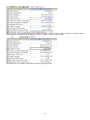
Features available vs. Versions
Personal
Base
Extended (**)
Database with more than 1600 chemicals
x
x
Database with more than 25000 BIPs
x
x
SRK, PR (vdW mixing rules)
x
x
x
SRK, PR (WS mixing rules)
x
x
x
LKP, BWRS, GERG, AGA, Steam Tables
x
x
x
UNIFAC,UNIQUAC,NRTL,Wilson
x
x
x
CPA (with association)
x
x
x
Solid Solution Model
x
x
x
SRK, PR (HV mixing rules)
E1
SRK, PR (MHV mixing rules)
E1
SAFT (with association)
E1
GERG (2008)
E1
BWR
E1
Pitzer , NRTL (electrolytes)
E1
Derivatives vs. P,T,W of Fg, H, S, V
x
x
Properties of fluids and mixtures
x
x
x
Vapor Liquid solid isothermal flash operation
x
x
x
Vapor Liquid Pf-T, Pf-P flash operations
x
x
x
Vapor Liquid solid H-P, S-P, V-P flash operations
x
x
x
Complete set of flash operations (Pf,H,S,V)
x
Vapor-Liquid phase diagram
x(*)
x
x
Vapor-Liquid-Liquid phase diagram
x (*)
x
x
Vapor-Liquid-Solid phase diagram
E2
VLE-LLE-SLE data regression
x
x
x
Raw data regression utility
x
x
x
Characterization of petroleum fractions
E2
Hydrate formation (multiphase with std. model)
x (*)
x
x
Hydrate formation (multiphase with complex model)
E2
Multiphase (gas,liquid) pipeline with heat transfer
E2
Isentropic nozzle HEM . HNE
x
x
Isentropic nozzle HNE-DS , NHNE
x
E2
Polytropic stage, single phase (gas)
x
Polytropic stage, multi phase (gas+liquid)
Distillation column (gas-liquid)
x (*)
x
x
x
x
x
x
Distillation column (gas-liquid-liquid and liquid-liquid)
E3
Depressuring unit (blow-down)
E3
Reactions
E3
(*) simplified procedures with limited features
(**) extended versions available with distribution license
6
Installing the program
this paraghaph provides information about system requirements, procedures on installing Prode Properties software and
upgrading from previous versions.
Sistem requirements
•
•
•
Microsoft Windows XP, Vista, 7, 8 or later compatible system
1GB of RAM installed (if used in union with Microsoft Excel or other applications)
20 MB of available hard-disk space
Installation procedure
1) download the last version of the program from Prode server :
http://www.prode.com
2) if there are previous installations of Prode Properties uninstall the previous version
3) run the program, the automatic installation procedure will do the work for you, follow the on-screen installation instructions
note : in some operating system you must be logged as a user with administrative privileges to make the necessary changes,
if you do not have administrative privileges, contact your system administrator for assistance.
To uninstall a Prode Properties installation
Use the Add / Remove Programs utility in the Windows Control Panel, the procedure does all the work for you.
Obtain the licence
Prode Properties is copy-protected, your personal copy has limited features and to access all the features you must obtain a
licence from Prode, there are se veral types of licence
• software copy protection (distribution via email, installation on a single computer identified by an installation code)
•
•
hardware (dongle) copy protection (we ship the dongle, installation on single or multiple computers )
network installation
Order a software copy protection licence
the licence file is based on the installation code which the program generates automatically.
•
Run an applications which does access Prode PROPERTIES, once in the Properties editor the licence page
will show the installation code ID (see below, it’s the string IGSGH2 )
•
when placing the order, specify the installation code
Order a hardware copy protection licence
There are versions for stand-alone computer and network-connected computers, please contact Prode for details
7
Prode Properties Quick Start
With Prode Properties you can solve complex problems with only minor programming effort. Much of the functionality is
provided by the library. In this chapter you will learn step by step how to access Properties from your favourite application. This
chapter is for those of you that want to skip the tutorial and immediately start using Properties. In the following sections, you will
learn how to utilize the samples provided with Properties. When you run the samples you will get a broad overview of the
possibilities available from using Properties, you will notice the following features:
• The Properties editor permits a simple and quick access and editing of all data including streams, units, databases.
• The user can define on each different stream : compositions, operating conditions , BIPs, thermodynamic models per
property (fugacity, enthalpy, entropy, volume)
• The Properties library solves problems as multiphase equilibrium, critical points etc.
• Specific methods are provided for diagnostic / error messages
• Results of flash operations, transport properties etc. can be retrieved easily into your application
Locating and testing the sample files
As default the sample files, including data files, project files, and other associated files are supplied with the program and
placed in subdirectories under Prode main directory.
MPORTANT
The installation procedure creates a directory \Prode\ and different subdirectories
\Prode\C
\Prode\Excel
\Prode\LIB
\Prode\MATLAB
\Prode\MATHCAD
\Prode\Fortran
\Prode\NET\VBprops
\Prode\NET\C#-props
includes definitions and code for C / C++ applications
includes samples for Microsoft Excel
includes the versions of the library
includes definitions and code for MATLAB applications
includes definitions and code for MATHCAD applications
includes definitions and sample code for Fortran applications
includes definitions and samples for Microsoft NET VB applications
includes definitions and samples for Microsoft NET C# applications
Data files folder
IMPORTANT
When running Properties requires to access several files, these are placed in a directory \Prode\ in user space to avoid possible
conflicts with code reserved areas, the exact path depends from Windows version and settings, for example in Windows XP
they could be placed in C:\Documents and Settings\All Users\Application Data, the list of files includes
chem.dat
pseudo.dat
bips.dat
mod.dat
def.ppp
res.lan
lic.dat
.........
do not remove or rename these files, if Prode Properties cannot access these files (for example because they have been
disseminated in different directories) an error message “Corrupted file, error reading data file” will be generated.
8
Getting Started from Microsoft Excel
IMPORTANT the different versions (32 or 64 bit) of Excel require different versions of Prode dll library,
(Excel 32 requires Prode dll 32 bit while Excel 64 requires Prode dll 64 bit),
when installing Prode Properties you must select the version suitable for your copy of Excel
IMPORTANT Microsoft Excel support files are located in the directory \Prode\Excel
IMPORTANT Define the proper separator (to be used in Macros) in Excel Reegional Settings, here we assume ‘,’ as separator,
you may wish to utilize a different separator, for eample =EStrGD(1;300;1.0E5) instead of =EStrGD(1,300,1.0E5)
IMPORTANT as first step you must load the add-in (file properties.xla) which instructs Excel about Prode Properties library, you
need to go through this procedure only once, to load the add-in
Excel 2003
open Excel and choose the Tools/Add-ins menu item, you’ll see a list of add-ins, some checked, some not checked. If Prode
Properties isn’t listed (and it won’t be unless you went through this procedure earlier) browse for the properties.xla file in Excel
folder then back your way out. Now Prode Properties should be listed in the list of add-ins, its box should be checked, and you
should see a Prode Properties menu in Excel. If you close Excel and then reopen it Prode Properties menu must still be there.
Once you installed the add-in you'll be able to access Prode Properties from within Excel (see below)
Excel 2007 and more recent versions
open Excel and choose Excel Options item, then Add-Ins, on the bottom select Manage Excel Add-Ins and click Go, you’ll see
a list of add-ins, some checked, some not checked. If Prode Properties isn’t listed (and it won’t be unless you went through this
procedure earlier) browse for the properties.xla file in Excel folder then back your way out. Now Prode Properties should be
listed in the list of add-ins, its box should be checked. If you click on Add-Ins you should see the Properties menu (see below).
Working with Excel
The Properties Add-In creates a menu which permits direct access to Properties Editor, save and load archives.
In Excel 2003 Properties adds a new item in main menu
In Excel 2007 to access Properties menu click on Add-Ins and then Properties
9
MPORTANT
Excel 2003 , Security Alert Macro
when opening Properties files in Excel 2003 you may be requested to fix a (Macro) Security Warning (see below ) issued by
Excel
To fix the Security Warning click Enable Macro in Security Alert dialog
Excel 2007 , Security Alert Macro
when opening Properties files in Excel 2007 you may be requested to fix a (Macro) Security Warning (see below “Security
Warning Macros have been disabled”) issued by Excel
To fix the Security Warning click the Options button and select Enable this content in Security Alert dialog
10
IMPORTANT
before to evaluate the sample files read the paragraph “Working with archives, save and load data, default settings”
while working in Microsoft Excel use the commands “Open Archive” and “Save a Archive” to save and restore data
IMPORTANT
the values indicated in this manual as results of some operations can be different when calculated with software due to the
different values of chemical’s properties and BIP’s stored in different versions of the software.
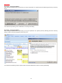
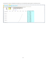
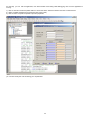
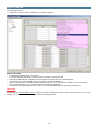
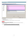
A simple way for accessing Prode Properties from Excel is to use the methods as macros within the cells, supposing we have
created a worksheet for solving some problem and we need the values of gas and liquid densities at some specified temperature
and pressure, first we need to define the stream and the units, from Properties menu select Edit Properties to define
compositions and the units of measurement .
Notice that for the first stream (for editing the different streams use the Select edit stream combo) there is a mixture of three
components already defined, you can change the list of components and compositions from Stream->components and models
from Stream->models.
MPORTANT
Once you modify a list of components it is recommended to edit also Models and BIPs dialogs, differently Properties adopts
default values.
If you modify something do not forget to click the Save button before to edit a different stream or leaving the dialog ! Differently
changes will be lost.
11
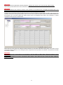
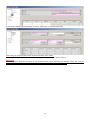
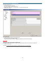
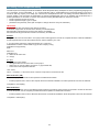
once defined the stream we need to define the units which we wish to utilize in our problem, for the pressure (first row) select
Bar.a , notice that unit for temperature is K and density Kg/m3 (but you can set the units which you prefer) then click on Ok for
accept changes and leaving the Properties editor
finally we can calculate the densities for the specified mixture directly in the cells, in B3 we enter the macro =EStrLD(1,B1,B2)
, for calculating liquid density of stream 1 at temperature specified in B1 and pressure specified in B2 ,in B4 we enter the macro
=EStrGD(1,B1,B2) for calculating the gas density and in B5 the macro =EStrLf(1,B1,B2) for calculating the liquid fraction
In B1 we enter 200 as temperature (remember we have K as unit) and in B2 we enter 5 as pressure (remember we have set
Bar.a as unit), densities are in Kg/m3 , notice that when you change B1 or B2 Prode Properties recalculates these values.
Now you can modify the stream 1 (changing the list of components, the compositions or models) or the units of measurement
and Prode Properties will calculate the value of ldensities and iquid fraction accordingly, in this way is very easy with Excel to
solve many different problems leaving to Prode Properties the task to calculate all properties for pure fluids and mixtures.
12
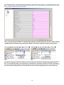
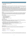
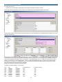
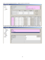
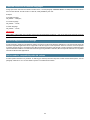
Next example permits to calculate the phase fractions and compositions in multiphase equilibria, to show the result in Excel
we’ll use a predefined Excel page, from Excel menu File->open , in Excel folder (in Prode Properties installation) select the file
multiphase.xls and click Ok to load the file
We need to define a new mixture :
a) from Properties menu select Edit Properties
b) in Stream->Operating dialog we select the stream number 2 and define the name “MIxture 2”
c) then we select t Stream->Components dialog and define a composition of two components with following molar fractions
Methane 0.9 n-Hexane 0.1
d) in Stfream->Models dialog we define SRK VDW (select in predefined packages) for both gas and liquid
e) we set Multiphase equilibria to Multiphase vapor-liquid and Multiphase initialization to Standard tests
f) then we can edit BIPs, we can input data or load from database
IMPORTANT when accessing the library from an external program you must define the proper settings in stream’s options for
multiphase flash operation
13
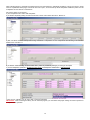
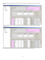
g) and finally in Stream->Operating dialog we click on Save button to save the stream data
Notice that once saved the dialog shows the feed composition of the stream.
Now you can define / access diferent streams as the program remembers your data for stream 2
MPORTANT
before to leave the application remember to save all data into the archive otherways your changes will be lost read the
paragraph “Working with archives, save and load data, default settings” for additional information
14
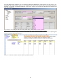
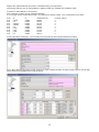
From the dialog Stream->Operating you can calculate a isothermal multiphase flash, select stream 2 as feed, then T-P VLL
(isothermal Vapor Liquid Liquid) , enter 187 K as temperature and 40 atm.g as pressure (this is the example provided by
Michelsen in “Calculation of multiphase equilibrium”) then click on Compute, the procedure will calculate two liquid phases and
show the compositions
If you wish you can modify the units from Config->Units dialog, define Bar.a as unit for pressure.
Notice that when changing units you must close and reopen the editor to see the changes (in editor).
The results are available directly in Excel, set stream as 2, temperature as 187 K and pressure as 4154420 Pa.a (40 atm.g) the
nclick on “Compute isothermal Flash at p,t”
Now you are able to calculate results at different operating conditions.
15
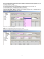
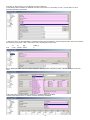
Altough a slow process multiphase analysis permits to discover instabilities and formation of new phases, examine the isothermal
flash at 149 K 10 Bar.a with API SRK as model and a mixture of Methane 0.7 Carbon Dioxide 0.15 Hydrogen Sulfide 0.15 , this
is the Mixture 1 provided as example.
a) from Properties menu select Edit Properties,
b) in Stream->Operating dialog select the stream number 1 , label “MIxture 1”
c) In Stream->Components verify the composition (Methane 0.7 Carbon Dioxide 0.15 Hydrogen Sulfide 0.15)
d) In Stream->Models we verify that model (fugacity) is SRK for gas and liquid
e) In Stream->BIPs we input BIPs or verify that procedure loads BIPs from database
f) in Stream->Components Save the stream
g) set as feed stream the first (“Mixture 1”), as operation T-P VL (isothermal, two phases flash), as specifications 150 K for
temperature and 10 Bar.a for pressure, then select Compute
The procedure detects one liquid phase,
a) define TP-VLL (isothermal vapor-liquid-liquid) and select Compute
NOTE
the procedure may detect two or three liquid phases depending from values of BIPs
16
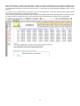
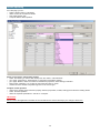
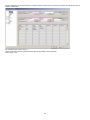
Next example permits to calculate and graph tables of values in a range of temperatures for many different properties (liquid
fraction, cp, cv, density, viscosity, thermal conductivity, speed of sound) and for both gas and liquid phases, for doing this we’ll
use a predefined Excel page, from Excel menu File->open , in Excel folder (in Prode Properties installation) select the file
props.xls
If you wish you can modify the stream composition or the units of measurement , in that case, as before from Properties menu
access the Properties editor and modify the previous data.
Then enter (in the proper units) the desired range of temperatures (cells B2-B3) and the operating pressure (cell B4) and click
on compute button to calculate the data, Prode Properties will print the values with the desired units of measuremebt.
17
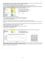
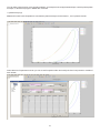
Next example will permits to calculate and graph a phase diagram ( phase envelope ), to do this we’ll use a predefined Excel
page, from Excel menu File->open , in Excel folder (in Prode Properties installation) select the file phasenv.xls
If you wish you can modify the stream composition or the units of measurement , in that case, from Properties menu access the
Properties editor and modify the previous data, remember to set the same equation of state for gas and liquid fugacity and dont’
forget to save the stream (button Save in first dialog) before to click “Ok” and exit. Then enter the desired liquid fraction for
equilibrium line (cell C6) and click on compute button to calculate the data, Prode Properties will print the calculated values with
the desired units of measurement, herebelow an example with 3 components
MPORTANT
The procedure for calculating a phase diagram allows different settings, you can modify these settings from the dialog Stream>Models (in Properties editor)
Check stability against feed option permits to test stability of calculated points against feed, unstable points are not printed, to
show all calculated points change the settings.
Phase diagram, specified phase fraction lines, allows to end (or continue) lines after crossing a phase boundary, set to end
(when crossing phase boundary lines) to avoid generating lines containing inconsistent data.
Phase diagram calculation option allows to select the EOS root for minimum Gibbs energy or according the state.
Hpwever the most important setting is the multiphase equilibria oprion which allows to calculate
1) vapor-liquid phase diagrams (see above)
2) vapor-liquid-liquid phase diagrams
3) vapor-liquid-solid phase diagrams
18
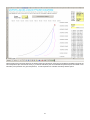
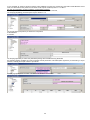
Next example will show a vapor-liquid-liquid phase diagram
a) In Excel load the file phasenv.xls
b) select the stream 4, a predefined test case with a natural gas mixture including water
c) click on compute button to calculate the data
Notice the water dew point line, the red line on the right
Next example will show a phase digram with up to three dew points at the same temperature,
a) In Excel load the file phasenv.xls
b) from Properties menu select Edit Properties,
c) in Stream->Operating dialog we select the stream number 2, a predefined test case
19
we can edit the list of components and the fraction of each component selecting the Stream->Components dialog,
this mixture includes two components with molar fractions Methane 0.999 n-Butane 0.001
we can modify models and options in Stream->Models dialog ,
in this test case we adopt Peng Robinson (PR-VDW) for both gas and liquid
we can edit BIPs from Stream->BIPs dialog
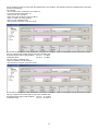
Remember, if you have changed some values, in Stream->Operating dialog click on Save button to save the stream data
for canculating the phase envelope for test case 3 from Excel page phasenv.xls
enter 3 as stream and 0.001 as liquid fraction and click on button “Compute phase diagram”
20
Observe that for this mixture the dew line, the red line below the critical point, shows up to three different equilibrium points at the
same temperature (the area around 190 K), if you add the saturation point on the bubble line (black line) we have atotal of four
saturation point pressures at a given temperature, Prode Properties can calculate accurately all these points.
21
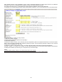
Prode Properties includes methods for calculating equilibrium points at specified conditions, see the paragraph “Methods for
thermodynamic calc’ s” for details, methods LfPF(), LfTF() as the name says are based on a liquid fraction specification, they
returns the first point (along the specified liquid fraction line) at the specified pressure (or temperature). Methods PfPF() and
PfTF() can accept a gas or liquid fraction (solid fractions in extended edition) as specification, they can calculate up to 5 points
(at specified pressure or temperature) along the line with specified phase fraction
double p = PfTF(integer stream, double t, double pf, int state, int n)
which requires the stream, the equilibrium temperature, the phase fraction (range 0-1), the state (gas, liquid, solid) and the
position (1-5) of the equilibrium point
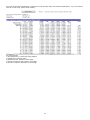
In cell B39 we define the temperature as 190.208 K , then in cells B40 , B41, B42 we enter the macros
=PfTF(3,B39,0,1,1)
in cell B40
=PfTF(3,B39,0,1,2)
in cell B41
=PfTF(3,B39,0,1,3)
in cell B42
where the first value (3) is the stream , the second (cell B39) represents the temperature, the third (1) is the phase fraction (with
1 we specify 100% gas or a point on dew line, the same would be by setting the state as liquid and phase fraction as 0.0) the
fourth (0) is the state (in Properties 0 = gas, 1 = liquid, 2 = solid) and the last is the required position (we require the points 13 along the dew line)
the procedure calculates the three equilibrium points, if we change the temperature to 190.1 K we get different equilibrium
pressures:
you may wish to test the method LfTF() , enter the macro
=LfTF(3,B39,0)
where 3 is the stream, B39 represents the temperature and 0 is the (liquid) phase fraction, notice that you’ll get the same values
as for the first equilibrium point in PfTF()
Finally we can calculate the point on bubble line with the method LfTF()
=LfTF(3,B39,1)
where 1 is the specification (100% liquid) for a point on the bubble line ,
of course you get the same result with the method
=PfTF(3,B39,1,1,1)
where the third value (1) is the phase fraction (with 1 we specify a 100% fraction) the fourth (1) is the state (in Properties 0 =
gas, 1 = liquid, 2 = solid) and the last is the required position for the point
22
Prode Properties includes several methods for solving multiphase (vapor-liquid-solid) phase equilibria plus enthalpy, entropy or
volume specifications
-specified enthalpy or entropy or volume and pressure
-specified enthalpy or entropy or volume and temperature
-constant energy and pressure
the paragraph “Methods for thermodynamic calc’ s” provides additional information.
in this example we will examine the methods HPF() and SPF() which permit to solve the enthalpy (HPF) or entropy (SPF) and
pressure specifications, they return the temperature at which the calculated value of enthalpy (or entropy) equals the specified
value.
These methods permit to solve many problems, for example
-model heat exchangers where you know inlet and outlet pressures and heat duty
-simulate valves where you know inlet and outlet pressures, usually valves are modeled as adiabatic processes (dh = 0)
-simulate pipelines where you know inlet and outlet pressures and heat exchanged with surrounding environment
-model pumps and compressors, when you know inlet and outlet pressures
Supposing we wish to simulate a process to cool down the mixture already examined in previous examples
Methane
Carbon Dioxide
Hydrogen Sulfide
0.7
0.15
0.15
with Soave Redlick Kwong model , from the point A in retrograde region and near the dew line (89 Bar.a and 246 K
to the point B located close to the critical point
this example can represent a good test for evaluating the stability and reliability of convergence in retrograde region
23
select stream 1 , verify the list of components and molar fractions (C1 = 0.7 CO2 = 0.15 H2S = 0.15) the models for vapor and
liquid fugacity (SRK VDW) and the values for BIPs
with these values the calculated p, t for critical point are 79.117 Bar.a and 232.08 K
In first dialog select the HP-VL flash operation on second grid, then set 89 Bar.a and 246 K as inlet conditions, 79.12 Bar.a as
outlet condition and -71.9 KW (-61864.3 Kcal/h) as heat duty, the negative sign means that energy is subtracted
Please note that you must specify the value of energy (to add or subtract) to the total value of stream determined as
specific enthalpy * mass flow the mass flow in this case has been specified as 1.0 Kg/s (see the second row)
Click on Compute buttom to solve the problem, the procedure calculates an outlet temperature (see the second row) of 232.1 K
which is close to the critical point giving a idea of reliability of procedure.
24
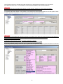
As alternative to utilize Properties Editor you can solve the problem directly in Excel,
in cell B5 enter EstrH(stream,p,t) to define the initial conditions for stream 1 at 89 Bar.a and 246 K and calculate the enthalpy
=EstrH(1,$B2,$B1)+$B4
where 1 is the stream, B2 is the operating temperature, B1 the operating pressure and B4 represents the additional duty
then with HPF() you calculate the final temperature at specified enthalpy (the initial enthalpy calculated at 89 Bar.a and 246 K
plus -or minus- the specified heat duty)
=HPF(1,$B3,$B5,0.0)
where 1 is the stream, B3 is the outlet pressure, B5 the required heat duty and 0.0 is the estimated final temperature (set to 0.0
for automatic initialization)
Prode Properties can solve multiphase equilibria (vapor, liquid, solid, hydrate) at specified value of enthalpy, entropy, volume
pressure , temperature, additional specifications are possible.
25
in next example we model a pressure reducing valve (adiabatic process), the stream has composition 0.982 Methane 0.018
CO2, the valve reduces the pressure from 200 K 37 Bar.a (inlet conditions) down to 1.72 Bar.a .
We wish to investigate if at outlet conditions a solid phase is present.
As first step we define a new stream with composition 0.982 Methane 0.018 CO2,
On first page (Operating) we select (first row) the stream nr. 10
On second page (Composition) we define the composition
0.982 Methane
0.018 CO2,
On third page (Models) we select the predefined package Soave Redlich Kwong Extended
the extended models available in Prode Properties include parameters calculated (data regression) for best fitting of vapor
pressure, enthalpy and liquid volume of pure fluids.
in fourth page (BIPS) click on button “Get BIPs from database” to load BIPs
26
We can model the pressure reducer with the predefined H-P VLS operation, this opetration solves a multiphase flash at specified
pressure and enthalpy.
On first page
-click on button Save to define the new stream 10
-in second grid select the stream 10
-select the H-P VLS operation
-define 200 K and 37 Bar.a as inlet conditions
-define 1.72 Bar.a as outlet pressure
-define 0 as dh (adiabatic flash)
-click on button “Compute” to get the results
the procedure calculates an outlet temperature of 157.45 K at 1.72 Bar.a , there is a solid phase (mainly composed by CO2)
We can compare these results against vapor-solid equilibria data
Experimental data (vapor-solid equilibria) 158.12 K , 1.72 Bar.a
Calculated values
157.45 K , 1.72 Bar.a
We can examine a different case
-define 15.72 Bar.a as outlet pressure
-click on button “Compute” to get the results
the procedure calculates an outlet temperature of 175.6 K at 15.72 Bar.a , there is a solid phase (mainly composed by CO2)
We can compare these results against vapor-solid equilibria data
Experimental data (vapor-solid equilibria) 176.04 K , 15.72 Bar.a
Calculated values
175.6 K , 15.72 Bar.a
27
In next example we estimate the (initial) discharging temperature of a fluid contained in a vessel protected by a safety valve, the
block valves have been closed and the fluid heated (at constant volume),
the mixture is that already examined in previous examples
Methane
Carbon Dioxide
Hydrogen Sulfide
0.7
0.15
0.15
with Soave Redlick Kwong model , the operating conditions are 60 Bar.a and 225 K
the discharging pressure is 78 Bar.a
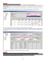
the method EStrV() in cell B3 allows to define the operating conditions and to calculate the specific volume
=EStrV(1,$B2,$B1)
where 1 is the stream, B2 is the inlet temperature and B1 is the inlet pressure
to calculate the Outlet temperature for the isochoric process in celll B5 we enter
=VPF(1,$B4,$B3,0)
where 1 is the stream, B4 is the final pressure, B3 the required specific volume (equal to inlet volume) and 0.0 the estimated final
temperature (the value 0.0 means we require the automatic initialization)
IMPORTANT due to the calling mechanism of Microsoft Excel in some cases Prode Properties may return a 0.0 value even
when a solution is available, in those cases you can get the correct results by forcing the cell recalc with the Enter key
28
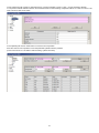
In next example we estimate the discharge temperature and the power absorbed by a single stage compressor with determined
adiabatic efficiency, the theoretical power requirements can be calculated as
(enthalpy at outlet conditions - enthalpy at inlet conditions) / mechanical efficiency
The outlet temperature is calculated with four steps,
a) model the compressor as isentropic process and calculate the final temperature
b) calculate the final enthalpy for the isentropic process
c) calculate the outlet enthalpy as
outlet enthalpy for the isentropic process - enthalpy at inlet conditions
outlet enthalpy = enthalpy at inlet conditions + -----------------------------------------------------------------------------------------------adiabatic efficiency
d) calculate the outlet temperature at given outlet enthalpy
The specifications are mass flow 1 Kg/s , fluid Methane 0.999, n-Butane 0.001 (this is the Test case 2) to compress from 10
Bar.a, 203 K to 20 Bar.a, we assume 0.75 as adibatic efficiency and 0.98 as mechanical efficiency
In Excel we define the inlet conditions with macro EStrH() which forces a isothermal flash at specified pressure and temperature
=EStrH(2,$B2,$B1)
where 2 is the stream, B2 is the inlet temperature and B1 is the inlet pressure
in cell B4 we calculate the initial entropy as
=EstrS(2,$B2,$B1)to calculate the outlet temperature for the isentropic process in celll B6 we enter
=SPF(2,$B5,$B4,0)
where 2 is the stream, B5 is the outlet pressure, B4 the required entropy (equal to inlet entropy being a isentropic process) and
0.0 as estimated final temperature
to calculate the outlet enthalpy enter in cell B7
=EstrH(2,$B6,$B5)
and in cell B9 enter
=$B3+($B7-$B3)/$B8
to calculate the final enthapy (with the adiabatic efficiency specified in cell B7),
to estimate the absorbed power in cell B11 enter
=($B9-$B3)/$B10
Since we know the enthalpy and pressure at outlet conditions we can calculate the temperature with HPF() method
=HPF(2,$B5,$B9,0)
where 2 is the stream, B4 is the outlet pressure, $B8-$B6 represents the heat duty (the difference from initial conditions calculated
in cell B6) and 0.0 the estimated final temperature
29
Now if we wish to evaluate the performance at different conditions we can modify the inlet conditions, for example setting
2500000 Pa.a as outlet pressure and changing the value in cell B1 or cell B2 to force a recalc
In a similar way you can define a procedure to model a polytropic process.
30
Next example shows how to simulate a compression stage (as polytropic process) where the inlet stream can be vapor or vapor
+ liquid (mixed), comparing the results of different methods, see the paragraph “Methods for solving a Polytropic operation”.for
additional information.
We use a predefined Excel page as interface to Prode Properties.
From Excel menu File->open , in Excel folder (in Prode Properties installation) select the file compressor.xls
the page contains two sections, the first permits to calculate the polytropic efficiency of a single compression stage given the
inlet temperature and pressure.
The second section allows to estimate the discharging temperature given inlet temperature and pressure, outlet pressure and
polytropic efficiency.
Notice that Prode Properties includes a specific methof for solving a polytropic stage with phase equilibria, this method permits
to simulate both single phase (vapor) and mixed (vapor + liquid) processes.
The mixture Methane 0.999, n-Butane 0.001 (predefined stream 2) at 10 Bar.a shows a dew point of 187.5 K , by setting a inlet
temperature of 180 K we specify vapor + liquid as inlet condition, the standard method can simulate only gas streams, however
the Polytropic solution with phase equilibria method allows to solve this case.
31
Next example allows to size a relief valve comparing the results of different methods for critical and two-phase flow, see the
paragraph “Methods for solving a Isentropic operation” for additional information.
We use a predefined Excel page as interface to Prode Properties.
From Excel menu File->open , in Excel folder (in Prode Properties installation) select the file nozzle.xls
The steps to size a relief valve are easy to follow:
1) from Properties editor define the composition, models, BIPs (for mixtures)
2) enter the discharging temperature, pressure, flow, model, outlet pressure
3) click on button “Calculate Solution”
the procedure calculates the required area and the outlet temperature for critical and two-phase flow,
you may utilize the procedure to verify the results from a different software in applications as fluids in critical area, two-phases
flow etc.
The same page includes a procedure to compare the results from HEM (Homogeneous Equilibrium) and different Non Equilibrium
models for a specified pressure in a range of inlet vapor qualities
Please follow fhese steps to compare:two models,
1) from Properties editor define the composition, models, BIPs (for mixtures)
2) enter the pressure, model and parameter
3) click on button “Compare Models”
.
The Non Equlibrium models are mainly of interest for short nozzles where the final equilibrium condition (predicted by HEM
models) is not reached cause the residence time of the fluid is too short.
The HNE models require specific parameters, for Prode HNE model a value of 0.75 is suggested for short nozzles but different
values may be defined to fit specific data sets.
32
Next example permits to solve a distillation column, refer to paragraph “Methods for solving staged columns” for additional
information, here we use a predefined Excel page as interface to Prode Properties methods.
From Excel menu File->open , in Excel folder (in Prode Properties installation) select the file column.xls
In this page you can define different kind of columns with reboiler, condenser , one or more feeds and one or more side streams.
The steps to define a column are easy to follow:
1) define the number of stages
2) define pressure distribution (bottom and top stage)
3) define stage efficiency
4) define the number of feeds, each feed flow rate and compositions (click on the proper Feed button to access the stream
editor), each feed stage (remember that reboiler (if present) is stage 1 and condenser (if present) is stage N, and the liquid
fraction (or the temperature) of each feed.
5) Define the number of side streams (if any) , the stage, the type (vapor or liquid flow) and the flow specification
6) Define variables as condenser and reboiler and the related specifications, the procedure allows different specifications
including molar fractions (and recovery) of a component in top or bottom stage
Notes :
In Stream Editor (Config->Units) you can define all the units for this project
in Stream Editor (Config->Setti gs) you can define mass units or molar units for flows in Stream Editor
33
Once the column has been defined it is suggested to verify the input data for inconsistent specifications, if you are sure that
all is Ok run the solver (button Solve Column)
the report includes
1) the verified errors in mass and energy balance
2) reboiler and condenser duties
3) temperature and pressure in each stage
4) total and component vapor flows in each stage
5) total and component liquid flows in each stage
34
next example shows how to calculate the hydrate formation curve (temperature and pressure) for a given mixture.
From Excel menu File->open , in Excel folder (in Prode Properties installation) select the file hydrate.xls
IMPORTANT
in order to calculate phase equilibria with hydrates you must include in stream one or more fomers plus water,
when solving multiphase equilibria Prode Properties considers SI, SII and SH structures
In Properties Editor select stream “6 Test Hydrate” in both selectors of first and second window, the “6 Test Hydrate” stream
includes a predefined composition C1 0.905 C2 0.05 C3 0.02 CO2 0.02 H2O 0.005 CH4O 0
IMPORTANT
when solving phase equilibria with solids and hydrates to avoid large errors make sure to have the same model selected for
vapor, liquid, solid and hydrate, you can set / inspect models from models tab in Properties Editor,
Base version allows two alternatives
1) CPA PR for vapor and liquid , SP-CPA for solid , HYD-CPA for hydrate
2) PR Extended (PRX) for vapor and liquid plus SP-PRX for solid and HPRX for hydrate
the list with predefined packages shows two opions, Hydrate CPA-PRX (based on CPA) and Hydrate PRX (based on Extended
Peng Robinson) , for this example select Hydrate CPA-PRX
35
IMPORTANT
solving hydrate phase equilibria you must define BIPs ,
Prode Properties includes many precalculated BIPs for VLE, LLE, SLE and Hydrates phase equilibria,
you may utilize these values when meaured data points are not available, if there are doubts about the range of application you
may inspect the database for the range of temperatures and estimated errors, see the paragraph “Binary Interaction Parameters
(BIP)” for details
Consider data regression from measured data the recommended option, for the details see the paragraph “Regress VLE-LLESLE data”
for this example select Hydrate BIPs as Data Set and click on Get BIPs from Database button to load the values
then, back to Operating tab and click on Save button to store the values in Prode Properties,
once saved you can calculate hydrate phase equilibria immediately selecting the TP VLSH flash operation, setting temperature
(277 K) and Pressure (15 Bar.a) , click on Compute button to see the results, at specified condotions the model indicates that
hydrates can form
you may decide to adopt methanol as inhibitor to avoid the formation of hydrates
IMPORTANT
depending from models BIPs for liquid-solid equilibria (water-methanol) may have limited ranges of application,
for the predefined BIPs included in Prode Properties (PRX model) the allowed range for the fraction methanol / water is 0.0-0.4
to keep the errors in calculated freezing point depression below 1.5-2 K in the range 210-273.15 K
if you wish to inject more methanol make sure to recalculate the liquid-solid BIPs with the utility available in Prode Properties,
for the details see the paragraph “Regress VLE-LLE-SLE data”
36
In this example we will consider a methanol fraction of 0.002 equivalent to 0.002 / 0.005 = 0.4 (the maximum allowed)
In component’s tab edit methanol fraction and methane fraction so that resulting composition will be C1 0.903 C2 0.05 C3 0.02
CO2 0.02 H2O 0.005 CH4O 0.002
in the Operating tab click on Save button to store the new composition
then solve the TP-VLSH operation to find the predicted hydrate formation pressure
(in this case we test 277 K 50 Bar.a without finding hydrate formation)
37
As alternative to solve the multiphase flash operations you can calculate the hydrate formation curve directly in Excel
38
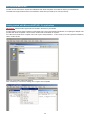
Getting started from MATLAB
IMPORTANT Microsoft MATLAB support files are located in the directory \Prode\MATLAB
MATLAB provides two ways to access external libraries as Prode Properties
-direct access
-access through scripts and mex files
Direct Access
Direct access is through the command-line interface, this interface lets you load an external library into MATLAB
memory and access functions in the library, to load Prode Properties in MATLAB enter
>if not(libisloaded('ppp'))
hfile = ['C:\Program Files\Prode\MATLAB\ppp.h'];
loadlibrary('ppp.dll', hfile);
end
libfunctions ppp
this command will load Prode Properties in memory and print the list of methods avaliable, you may wish to modify
‘C:\Program Files\Prode\MATLAB\ppp.h' to reflect your installation’s settings
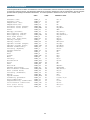
Functions in library ppp:
AFOpen
AFSave
AOpen
ASave
BFsave
BPF
BPLine
BRegr
CompAc
CompCID
CompDm
CompF
CompGC
CompGV
CompGf
CompHG
CompHL
CompHS
CompHV
CompHf
CompID
CompLC
CompLD
CompLV
CompMp
CompMw
CompN
CompNb
CompPc
CompRg
CompSC
CompSD
CompSG
CompSL
CompSS
CompST
CompSf
CompSol
CompTc
CompVP
CompVc
DCOL
DPF
DPLine
Divi
EStrFMH
EStrFML
EStrGC
EStrGCp
EStrGCv
EStrGD
EStrGIC
EStrGJT
EStrGMw
EStrGSS
EStrGV
EStrGVE
EStrH
EStrHC
EStrLC
EStrLCp
EStrLCv
EStrLD
EStrLIC
EStrLJT
EStrLMw
EStrLSS
EStrLV
EStrLVE
EStrLf
EStrPf
EStrS
EStrSCp
EStrSD
EStrST
EStrZv
ErrMsg
GSep
HPF
HPFORM
HTF
HTFORM
LFLine
LSep
LfPF
LfTF
MixF
PIPE
PSep
PfPF
PfTF
SPF
STF
StrAc
StrCBp
StrCBt
StrCPnr
StrCTp
StrCTt
StrCopy
StrFMH
StrFML
StrFv
StrFvd
StrFvdv
StrGC
StrGCp
StrGCv
StrGD
StrGH
StrGIC
StrGICp
StrGJT
StrGMw
StrGS
StrGSS
StrGV
StrGVE
StrH
StrHC
StrHv
StrHvd
StrLC
StrLCp
StrLCv
StrLD
StrLH
StrLIC
StrLJT
StrLMw
StrLS
StrLSS
StrLV
StrLVE
StrLf
StrMDt
StrMw
StrN
StrPc
StrPcm
StrPf
StrPt
StrPts
StrS
StrSCp
StrSD
StrSGH
StrSGS
StrSH
StrSLH
StrSLS
StrSS
StrSSH
StrSSS
StrST
StrSv
StrSvd
StrTc
StrTcm
StrVv
StrVvd
StrZv
StrlnFv
StrlnFvd
StrlnFvdv
UMAU
UMCR
UMCS
UMRAU
VLLSep
defErrMsg
edCF
edCS
edS
edSS
edST
getAji
getCC
getCNr
getCi
getCj
getErrFlag
getFCNr
getFPNr
getGij
getGji
getKji
getMBPNr
getMCNr
getMFg
getMH
getMS
getMSNr
getMV
getMod
getOM
getP
getPNr
getPatm
getSUMS
getT
getUMC
getUMN
getUMS
getW
getWm
getX
getY
getZ
initS
isSDef
loadSB
putAji
putBIP
putCC
putCi
putCj
putGij
putGji
putKji
putMod
putN
putZ
setAc
setErrFlag
setKM
setMFg
setMH
setMS
setMV
setMw
setOM
setOp
setPc
setS
setSOp
setTc
setUMC
setVc
setWm
to access a method in a shared library MATLAB provides the command calllib to call functions in the library, the syntax
for calllib is:
calllib('ppp', 'FunctionName', arg1, ..., argN)
the FunctionName and arguments are detailed in Prode Properties manual, for example we can call the method
edSS() to edit streams with the command
>calllib('ppp', 'edSS')
in the same way you can access other methods in Prode Properties, for example to calculate cp / cv and speed of
sound for vapor fraction of stream 1 at 300 K and 5 Bar
>> calllib(‘ppp’,’EstrGCp’1,300,500000)/’calllib(‘ppp’,’EstrGCv’1,300,500000)
>> ans = 1.3211
>> calllib(‘ppp’,’EstrGSS’1,300,500000)
>> ans = 374.1625
you can call even complex functions as those to plot a phase envelope or calculate a column, for these remember
before to pass an array from Matlab to Prode Properties that you must allocate the memory to avoid system errors.
Finally you can use the unloadlibrary function to unload Prode Properties library from Matlab and free up memory.
>unloadlibrary ppp
39
Access from Matlab through scripts
In addition to direct access, you can utilize Prode Properties from Matlab with scripts or mex files (compiled scripts)
In many cases this way is more immediate since you use the original names of the functions in Prode Properties
without need to write additional code.
Prode Properties includes a large number of Matlab scripts installed in directory \Prode\MATLAB\m
Before to utilize the scripts you must
-move the files into a Matlab directory (i.e. a directory where Matlab can access the scripts) , read Matlab documentation for additional information.
-edit the file pppdir.txt, this file contains a string with path and name of the header file required to instruct Matlab about
the methods avalialable in Prode Properties library, once you have edited move the file on the same location of script
files.
How the scripts work
Scripts act as interface between Matlab and Prode Properties, scripts have names identical to Prode Properties methods, then when you invoke the script StrGD (which is the method in Prode Properties to calculate density of vapor
phase) MATLAB simply executes the commands found in the file, calls the method StrGD in Prode Properties and
returns the result, by the way the script StrGD.m contains these MATLAB commands
function [] = StrGD(stream)
if not(libisloaded('ppp'))
fid = fopen('pppdir.txt'); hfile = fgetl(fid); fclose(fid);
loadlibrary('ppp.dll', hfile);
h = uimenu('Label','Properties');
h1 = uimenu(h,'Label','Edit Properties','Callback','edSS');
h2 = uimenu(h,'Label','Open Archive','Callback','AOpen');
h3 = uimenu(h,'Label','Save a Archive','Callback','ASave');
end
d = calllib('ppp', 'StrGD', stream)
end
By typing in Matlab the command
>>StrGD(1)
Matlab executes the code within the script, it loads ppp.dll (if not in memory) , creates a menu bar (with the standard
Prode Properties commands) and then executes the method StrGD, to calculate the density.
Notice that the script creates a menu bar which permits to access directly Prode Properties from Matlab GUI,
there are three commands
-edit Streams
-open a archive
-save a archive
Important features of menu bar
-the characteristics may depend from Matlab version
-if you delete the associated figure the menu bar is deleted, to recreate the menu you must reenter the commands
h = uimenu('Label','Properties');
h1 = uimenu(h,'Label','Edit Properties','Callback','edSS');
h2 = uimenu(h,'Label','Open Archive','Callback','AOpen');
h3 = uimenu(h,'Label','Save a Archive','Callback','ASave');
40
You can write scripts to solve more complex problems, an example is the script phaseenvelope.m which prints a phase
envelope, to test the script type in Matlab the command
>>phaseenvelope(1)
Matlab will invoke Prode Properties to calculate the phase envelope for the stream 1 , then it plots the result
Notice that from Properties menu bar you can access Properties editor and modify the list of components or models of
each stream
41
Access from MATHCAD
The files and the instructions required to link MathCad with Prode Properties are located in directory \Prode\MathCad
The MathCad support files and the documentation have been provided by Dr. Harvey Hensley
Getting started with Microsoft NET (VB , C) applications
IMPORTANT Microsoft NET support files are located in the directory \Prode\NET
Prode Properties can be easily included as unmanaged code in every Microsoft NET application, for compiling the sample code
provided with Prode Properties a recent version of Microsoft Visual Studio is required.
From Microsoft Visual Studio compiler menu File->Open->Project/Solution , in NET folder (in Prode Properties installation)
select the file vba.sln
then from menu Build- select Build Solution.
Note: if desired you can edit the settings from Project->vba Properties
42
As next step you can test the application, from Visual Studio menu Debug->Start Debugging, then once the application is
running :
1) click on the button Prode Properties editor to access the editor, define the streams and units of measurement
2) define a suitable temperature and pressure (with proper units)
3) click on button Compute Properties to print the properties
you can then modify the code according your requirements.
43
Solving problems (introduction)
There are several different classes of problems which Prode Properties can help to solve but the most common are probably :
• physical properties of pure fluids and mixtures
• equipment design
• system simulation
Prode Properties provides many methods for the prediction of physical properties, in general a single instruction is required for
calculating a property.
The design and rating of unit operations as distillation columns, towers, pumps, compressors, valves, heat exchangers etc. is
another area where Prode Properties can result useful, the use of programming languages is generally suggested when
dealing with complex problems while some formula in a worksheet can solve the usual work.
The system simulation may be used in the design stage to evaluate parameters, to help achieve an improved design or applied
to existing systems for optimizing operating conditions. Generally the required solution is the list of operating conditions at the
input and output of the operating blocks in the simulation block diagram. When there are no recycle streams or controls the
method for solving the system is very simple : the output information from the first operating block is utilized as input for the
second operating block and so on. However when there are output conditions which may interfere with input conditions some
sort of iteration is required since some or all the equations governing the system may be non linear. There are two well known
methods for solving such a system of non linear equations, the method of successive substitutions and Newton-Raphson, refer
to good books of numerical analysis for additional information.
Streams
Most thermodynamic calcs in Prode Properties library take as reference a stream entity. For example when simulating a plant
it makes sense to define different streams to represent flows in different sections, a stream usually defines compositions
and operating conditions, Prode Properties supports a variable number of streams and most methods in Prode Properties
require a reference to a stream, the reference is a numeric code (a progressive integer starting from 1 for first stream) .
Streams attributes
As
•
•
•
•
•
•
in process simulators each stream may include following information
a list of components and relative weights
a value for the operating pressure
a value for the operating temperature
a value for the operating flow
thermodynamic models for different properties
a list of BIPs
Working with streams
Prode Properties permits to define complex topologies as there is no limit to the number of operating blocks required for
simulating a plant, with Prode Properties for simulating a plant you convert the different sections into pieces of code, to do
so you can use the basic blocks available in all process simulators, for esample
• isothermal flash, for calculating multiphase equilibria at the specified temperature ad pressure
• flash unit (enthalpy, entropy or volume basis), calculates output temperature or pressure, with this unit you can simulate
pipelines, valves, heat exchangers, pumps, compressors and many others operations.
• fixed vapor fraction flash, for constructing phase envelopes, calculating bubble and dew points etc.
• mixer to add the contents of two streams
• divider to subtract a part of flow from a stream
by putting together these blocks it is possible to simulate also complex plants.
Simulating a plant
transform the flow sheet in a simulation block diagram, fluid and energy flow diagrams are standard engineering tools, you
assign a number to the different streams and identify the basic blocks which will be solved by Prode Properties.
Notice the number which identifies each stream, in this case different numbers mean (possible) different compositions (we do
not consider chemical reactions here), the output of each block can be easily calculated providing the input has been defined
44
Working with archives, save and load data, default settings
Load and save archives
Archives are files which contain the data required by Prode Properties to work with stream's and units of measurement, when
you open an archive the stream's data and units are loaded, when you choose to save an archive these data are stored in a file,
in this way you can work with many different projetcs.
Prode Properties includes several methods to save and load data as archives.
The default settings
When Prode Properties starts it loads data from the archive named "def.ppp" so if you wish to use your own list of streams,units
etc. just save your preferred settings under the name "def.ppp".
Properties editor
Prode Properties includes Properties editor, from the editor you have access to
• Streams
edit operating conditions, flow, compositions, models, BIPs for all streams
• Config
edit all units of measurement and settings
• Chemicals edit all chemical’s data, regress data , add new chemicals
• BIPs
edit BIPs, regress data, add new BIPs
How to activate the Properties editor
call one of the methods edS(stream), edSS() remember that in Prode Properties each stream is referenced with a code (integer
value) in the range (1... max number of streams).
Use the right method :
Use edSS() if you wish to start editing the first stream (but access all streams).
Use edS()stream if you would like to choose which stream to edit
From Microsoft VB
Call edSS()
Call edS(8) ‘ start editing stream nr. 8
From Microsoft Excel
=edSS()
=edS(8) ‘ start editing stream nr. 8
From Microsoft Visual C++
edSS();
edS(8); // start editing stream nr. 8
45
Stream operating
From this page you can :
• select a stream (select / edit stream)
• define a name for the selected stream
• save edited stream data
• Compute different flash operatins
Define a new stream / edit existing streams
• select the stream (you wish to edit / define) from the “Select / edit stream list”
• go to page “Components”, define the list of components and relative weights
• go to page “Models”, define the models for the different properties, define settings, load BIPs
• back to page “Operating”, put a name for the stream and click on “Save”
• check that correct stream composition appears on the second grid
Compute a flash operation
• make sure a feeding stream has been properly defined (composition, models, settings) then select the feeding stream
• select the flash operation
• define the required specifications and clik on “Compute”
IMPORTANT
before to leave the application remember to save all data into the archive otherways your changes will be lost !
46
Predefined Flash Operations
Prode Properties allows to solve directly from editor many Flash operations
T-P VL
vapor-liquid, two phases, at specified temperature and pressure
T-P VLL
vapor-liquid-liquid, multiphase, at specified temperature and pressure
T-P VLS
vapor-liquid-solid, multiphase,at specified temperature and pressure
T-P VLSH
vapor-liquid-solid-hydrate, multiphase,at specified temperature and pressure
LF-P
equilibrium temperature at specified (liquid) phase fraction and pressure
LF-T
equilibrium pressure at specified (liquid) phase fraction and temperature
H-P VL
equilibrium temperature, two phases, at specified pressure and enthalpy
H-P VLL
equilibrium temperature, vapor-liquid-liquid, multiphase, at specified pressure and enthalpy
H-P VLS
equilibrium temperature, vapor-liquid-solid, multiphase, at specified pressure and enthalpy
H-P VLSH
equilibrium temperature, vapor-liquid-solid-hydrate, multiphase, at specified pressure and enthalpy
S-P VL
equilibrium temperature, two phases, at specified pressure and entropy
S-P VLL
equilibrium temperature, vapor-liquid-liquid, multiphase, at specified pressure and entropy
S-P VLS
equilibrium temperature, vapor-liquid-solid, multiphase, at specified pressure and entropy
S-P VLSH
equilibrium temperature, vapor-liquid-solid-hydrate, multiphase, at specified pressure and entropy
V-P VL
equilibrium temperature, two phases, at specified pressure and specific volume
V-P VLL
equilibrium temperature, vapor-liquid-liquid, multiphase, at specified pressure and specific volume
V-P VLS
equilibrium temperature, vapor-liquid-solid, multiphase, at specified pressure and specific volume
V-P VLSH
equilibrium temperature, vapor-liquid-solid-hydrate, multiphase, at specified pressure and specific volume
Copy Stream
copy a stream into another stream
Gas Separator
simulates a gas separation at specified temperature and pressure
Liquid Separator
simulates a liquid separation at specified temperature and pressure
47
Stream Composition
From this page you can :
• define a list of components by selecting components from the library
• specifyi the amount of each component.
Define the sorting criteria
• select the preferred criteria
Add a component to the list
• select a component from the list of components
• click on Add button
Remove a component from the list
• click on Remove button to remove the last component in the list
Clear the list
• click on Clear button to rclear all components in the list
Enter / normalize according Mole or Weight fractions
•
select the desired Mole or Weight fractions
MPORTANT
to obtain the maximum accuracy solving multiphase equilibria with solid and hydrate phases it is suggested to regress BIPs from
VLE + LLE data points, models such as CPA-PR can calculate accurately fugacities of solid phases with a suitable set of BIPs.
48
Stream Models
From this page you can :
• define up to 30 different packages with user defined models and options
• define the model per each propertty and state (gas,liquid,solid)
• set different options available for calc’s
Define a new package / Edit existing package
• select a package in the list
• in Models and Options Window select the models and options for this package
• define a name for the package,
• click on “Save” button to save this package
Select a package
• select a predefined package in the list
Define a model
• specify the model per each property and state
Set a option
• define multiphase as vapor + liquid or vapor +liquid+solid
• reduce the number of trial phases (in multiphase)
• use iso compressibility coeff. to detect the state of each phase
• evaluate stability of each phase in equilibrium
• in phase diagrams, end lines with specified phase fractions when crossing a phase boundary
• in phase diagrams, select EOS root for minimum energy or state
49
BIPs
From this page you can :
• input / edit / load BIPs for the different models
Define a list of BIPs
• click on Get BIPs for loading all BIPs available in library
• if required add your own specific BIPs
IMPORTANT
For BIPs the first two columns Ci and Cj define the component’s position in the list (i.e. 1 for the first component , 2 for second
and so on), while othe colums allow to enter the values for the different BIPs required by selected model, note that some values
(for example in Wilson, NRTL etc.models) have units of cal / gr.mol.
Example, binary of methanol and ethyl acetate UNIQUAC A12 : -64.1299, A21 : 644.1931 in the first two columns (c1 , c2) enter
the components relative position in the list, assuming that methanol is the first component and ethyl acetate the second
c1
1
c2
2
BIP-1
-64.1299
BIP-2
644.1931
MPORTANT
Prode Properties allows to define Temperature Dependent BIPs for models as Soave or Peng Robinson, Temperature Dependent
BIPs provide a better accuracy than Temperature Independent BIPs, the database includes many Temperature Dependent
BIPs, BIPs in database have been calculated from VLE points at temperatures about 300 K and may not produce reliable results
at temperatures far from 300 K, in those cases (a typical application could be a phase envelope) it is recommended to use
Temperature Independent BIps or calculate new BIPs for the required range of temperatures.
50
Config Units
From this page you can :
• define the unit of measurement for the different properties
IMPORTANT
Prode Properties is a collection of functions for thermodynamic calculations, these functions receive data, of properties such as
temperature or pressure, a reference to a stream etc. and perform some operations.
With Prode Properties you have complete control over the engineering units, this means that program permits to select from a
list of different units for each property, and Prode Properties automatically converts the input values and the results according to
the selected units.
1) if you set Bar.a as unit for pressure all inputs and outputs will be in that unit !.
2 ) if you wish to define your own set of units remember, before to leave the application, to save data into a archive otherways
your changes will be lost !
51
Config Settings
From this page you can :
• define the different settings as max number of streams, the temperature and pressure at reference conditions, the base
values for entalpy and entropy, convergence tolerance etc.
Prode Properties permits to define several different operating parameters, these parameters are :
•
•
•
•
•
•
•
•
•
max number of streams
max number of components per stream
max number of interaction coefficients pairs per stream
reference temperature and pressure
base values for enthalpy and entropy calc’s
convergence tolerance
max allowed time for solving a operation
Flow units
minimum liquid density to validate liquid phase
IMPORTANT
before to leave the application remember to save all data into the archive differently your changes will be lost !
52
Chemicals data
From this page you can :
• edit and change the physical properties data included in the databank
• save all data in a file
Edit / modify data :
• select a component from the component’s list
• edit / modify the related fields (see also the section with description of all fields)
• select the “Save” button to save the modified data (differently new data will be discharged)
Adding a new component :
•
•
•
select the “New” button
edit the related fields (see also the following page with description of all data fields)
select the “Save” button to save the data (differently new data will be discharged)
Remove a component :
•
•
select a component from the component’s list
select the “Remove” button
IMPORTANT
Updating the file which contains the databank :
this option permits to store all data into a file, differently all changes will be lost when leaving the application
• select the “File” button
CAUTION : you may wish to create a backup of the file chem.dat before to overwrite the file
53
Chemicals Settings
From this page you can :
• edit informations (CAS number) required to identify some components .
54
Regress raw data
From this page you can :
• regress raw data into values compatible with chemical’s database
Regress raw data
•
•
•
•
•
•
•
in Chemicals Data page select a chemical
in Chemical Regress page selet a property and the correlation for fitting raw data
enter the available data (all temperature and value pairs) with the proper units of measurement
if required you may enter initializing values and limits for calculated parameters
click on Calculate button, evaluate calculated values and errors, you may try different correlations for best data fitting
click on Transfer button to copy calculated values into Chemicals Data page
in Chemicals Data page select the “Save” button to save the data (differently new data will be discharged)
IMPORTANT
Prode Properties flexible datbase format supports more than 15 different correlations (30 in extended version), so for each
property you can select the correlation which best fits experimental data.
55
Binary Interaction Parameters (BIP)
From these pages you can :
• edit Binary Interaction Parameters
• add / remove Binary Interaction Parameters
• regress VLE (vapor-liquid) , LLE (liquid-liquid) , SLE (solid-liquid) data points
• save all data in a file
Edit / modify data :
• select two components from the component’s lists
• edit / modify BIPs for the different models
• select the “Save” button to save the modified data (differently new data will be discharged)
IMPORTANT
Updating the file which contains the BIPs data :
this option permits to store all data into a file, differently all changes will be lost when leaving the application
• select the “File” button
CAUTION you may wish to create a backup of the file bips.dat before to overwrite the file
56
Regress VLE-LLE-SLE data
From this page you can :
• regress VLE-LLE-SLE data for calculating the best fitting paraneters of different models
as first step in BIPs->Data page you must select two components (in this example methanol and water)
The procedure permits to enter experimental (measured) VLE-LLE-SLE data points or fit automatically the model to VLE points
calculated with UNIFAC.
When entering measured VLE (vapor-liquid data points) on each row include in X column the measured liquid molar fraction
of component 1, in Y column the measured vapor molar fraction of component 1, for LLE (liquid-liquid equilibria) include in X
column the measured liquid molar fraction of component 1 in first liquid phase, and in Y column the measured liquid molar
fraction of component 1 in second liquid phase, for SLE (solid-liquid equilibria) include in X column the measured liquid
molar fraction of component 1 in liquid phase, and in Y column the measured solid molar fraction of component 1, finally
enter the temperature and the pressure for that point.
Example of measured VLE data for Methanol-Water
VLE data for Methanol-Water at 735 mmHg
Point
VLE
VLE
VLE
VLE
VLE
VLE
VLE
VLE
X(1)
0.008400
0.025800
0.068000
0.137000
0.240000
0.480000
0.572000
0.741000
Y(1)
0.103000
0.227000
0.391000
0.568000
0.680000
0.790000
0.820000
0.906000
Temperature (C)
96.5
92.3
87.5
80.1
75.9
70.6
68.7
66.4
Pressure (mmHg)
735
735
735
735
735
735
735
735
57
Enter the measured data, select the models to regress (in this case Wilson for liquid phase and regulat -ideal- for vapor
phase)
Selecting the button Calculate the procedure calculates the best fitting parameters, shows the calculatd results and the
relative errors (%)
as alternative the procedure offers the option to calculate the best fitting parameters to VLE data points calculated with UNIFAC,
this entirely predictive method doesn’t require experimental data and in some cases can result useful.
58
Select “VLE points calculated with UNIFAC” in “Regress” selector to use this method
Once the paramters have been calculated you must select the “Transfer” button to transfer the results in BIPs->Data page, from
that page you can save the calculated BIPs in database (select Save button) or store permanently in file (select File button).
59
Regress SLE (Water-Methanol) and test the calculated freezing point depression
This example will show how to estimate BIPs for different models from available SLE equilibrium points
SLE data for Water-Methanol atm pressure
First component is Water, second component Methanol
X1 is the water fraction in liquid phase while Y1 is solid fraction (always 0.9999... for a model based on pure fluid)
Point
SLE
SLE
SLE
SLE
SLE
SLE
SLE
SLE
SLE
X1
0.9432
0.9
0.87676
0.80583
0.8
0.728
0.641
0.636
0.6
Y1
0.9999
0.9999
0.9999
0.9999
0.9999
0.9999
0.9999
0.9999
0.9999
Temperature (K)
266.85
259.65
257.65
246.85
242.95
233.45
217.95
214.95
208.15
Pressure (Bar.g)
0
0
0
0
0
0
0
0
0
as first step in BIPs->Data page you must select the components (in this example methanol and water)
then in BIPs->Regress page select models (CPA-PR for vapor, CPA-PR for liquid, SP-CPA for solid) options, enter all data
points and click on Calculate button to get the results
60
Then click on Save button to move calculated values on Data tab,
in Data dialog select SLE BIPs as database and click on Save button to store data, you may use File button to store
(permanently) data in bips.dat file
to test the accuracy of calculated BIPs in estimating freezing point depression in Prode Properties Editor select a new stream
and define as composition H2O 0.728 CH4O 0.272 to test this point in the series
SLE
X1
0.728
Y1
T(K)
0.9999 233.45
P(Bar.g)
0
then in Models tab select the same models adopted in data regression, CPA-PR for vapor, CPA-PR for liquid, SP-CPA for
solid
In BIPs tab select SLE BIPs Data set and click on Load BIPs button to get BIPs,
make sure that values shown on window are those previously calculated
61
Finally in Operating tab click Save Button to define the stream and solve a TP-VLS flash operation to evaluate the point of
incipient solidification
the calculated point is about 235.1 K ,
compare this value with the experimental data (233.45 K) utilized in data regression,
error is about 1.6 K
62
Parameters of models
From this page you can :
• edit the parameters required by the different models available in library
Edit / modify data :
• select the components from the component’s lists
• select the model
• edit / modify the parameters
• select the “Save” button to save the modified data (differently new data will be discharged)
IMPORTANT
Updating the file which contains the Model data :
this option permits to store all data into a file, differently all changes will be lost when leaving the application
• select the “File” button
CAUTION you may wish to create a backup of the file bips.dat before to overwrite the file
63
Accessing Prode Properties library
The technique for accessing the methods available in Prode Properties library will depend on which programming language You
use. Languages such as FORTRAN , C, C++ or Microsoft NET (VB,C) exhibit differences in parameter passing in and out of
functions. This may require you to adapt your code from the examples shown here. The calling convention determines how a
program makes a call and where the parameters are passed. PROPERTIES does use of standard calls of Windows API, it
pushes parameters on the stack, in reverse order. When accessing PROPERTIES You must also consider :
• Prode Properties real type is 8 bytes
• Prode Properties integer type is 4 bytes
• parameters are passed by value (with exception of strings which are arrays of characters)
IMPORTANT
C / C++ support files are located in the directory \Prode\C
FORTRAN support files are located in the directory \Prode\FORTRAN
Microsoft NET support files are located in the directory \Prode\NET
Microsoft EXCEL support files are located in the directory \Prode\Excel
Fortran
add ppp.lib file to the list of the files in Your project and include ppp.f90 to instruct the compiler about the methods available in
Prode Properties then access the methods as they were included in your code
C this procedure returns the critical temperature of a compound
INTERFACE TO REAL*8 FUNCTION TC ([C,ALIAS:’CompTc’] comp)
INTEGER*4 comp [VALUE]
END
REAL*8 tc
INTEGER*4 id
C define the id value here
tc = TC(id)
C / C++
•
•
•
•
include the ppp.h header
add ppp.lib file to the list of the files in Your project
make sure you use the calling convention of ppp.h header file,
access the Prode Properties methods
char *name;
name = CompN(1); // returns the name of the first component in the chemical’s file
Microsoft NET ( VB )
see the samples provided with Prode Properties for additional information
•
include properties.vba to instruct the compiler about the methods available in Prode Properties and access the methods
CompName = MCompN(1)
Microsoft Excel
Microsoft Excel supports macros and VBA language for defining procedures; both of these can be used to access the functions
in Prode Properties, see the samples provided with Prode Properties for additional information
•
include properties.vba to instruct Microsoft Excel about the methods available in Prode Properties and access the methods
CompName = MCompN(1)
64
Translate resources to different languages
A large part of the resources are stored in the file res.lan , see the paragraph “Data files folder” for additional information about
how to locate the file. The file res.lan is a text file, easily editable by the user.
Example
in English language
N2_NAME = “Nitrogen”;
in French language
N2_NAME = “Azote”;
in Italian language
N2_NAME = “Azoto”;
IMPORTANT
When editing a string take care to modify only the parts enclosed within the braces ”” and do not alter/modify the data structures
composed by special characters as for example ::
Microsoft Applications and Strings
Prode Properties utilizes the standard API calling convention for Microsoft Windows applications. This assures that almost all
Windows compatible applications which support DLLs will also support Prode Properties. There are, however, some exceptions
in passing strings (arrays of characters) since Microsoft utilizes proprietary data formats. Prode Properties includes Microsoft
specific methods in addition to the standard methods supporting the ANSI C standard, Microsoft specific methods are compatible
with almost all Microsoft applications.
Define models, compatibility with old verions
Prode Properties includes many methods for defining (via software) the thermodynamic models and the related options, see the
paragraph “Methods to set / access different options” for additional information
65
Units of measurement
Prode Properties allows to define via software the units of measurement, there are methods for defining the units and methods
for retrieving codes and strings, see paragraph “Methods for accessing / defining the units of measurement” and the samples
provided with the package for additional information, in Prode Properties to reference a unit must use a numeric code
QUANTITY
UNIT
Pressure (abs)
Pressure (rel)
Temperature (abs)
Temperature(rel)
Calorific Value (weight)
Calorific Value (molar)
Power
Entropy (Streams)
Heat Capacity (weight)
Heat Capacity (molar)
Flow (mass basis)
Flow (gas, mass basis)
Density (weight)
Density (molar)
Specific Volume (weight)
Specific Volume (molar)
Thermal Conductivity
Viscosity (dynamic)
Surface Tension
Lenght
Area
Volume
Mass
Velocity
Acceleration
Force
Time
Heat Flux
Thermal Resistance
Heat Transfer Coefficent
Flow (volume basis)
Viscosity (kinematic)
Energy
Dipole moment
Solubility parameter
Flow Coefficient
Compressibility coefficient
Joule Thomson coefficient
Flow (molar basis)
Volume expansivity
CONV_P
CONV_DP
CONV_T
CONV_DT
CONV_HM
CONV_HMM
CONV_HS
CONV_SS
CONV_CP
CONV_CPM
CONV_W
CONV_WG
CONV_D
CONV_DM
CONV_SV
CONV_SVM
CONV_TC
CONV_V
CONV_ST
CONV_L
CONV_A
CONV_VOL
CONV_M
CONV_VL
CONV_ACC
CONV_FOR
CONV_TM
CONV_HF
CONV_TR
CONV_HTC
CONV_VW
CONV_VK
CONV_EN
CONV_EDM
CONV_SP
CONV_CV
CONV_CC
CONV_JTC
CONV_WM
CONV_VE
CODE
15
16
17
18
19
20
21
22
23
24
25
26
27
28
29
30
31
32
33
34
35
36
37
38
39
40
41
42
43
44
45
46
47
48
49
50
51
52
53
54
66
DEFAULT UNIT
“Pa.a”
“Pa”
“K”
“K”
“Kj/Kg”
“Kj/Kmol”
“KW”
“KJ/(K*s)”
“kJ/(kg*K)”
“kJ/(kmol*K)”
“Kg/s”
“Kg/s”
“Kg/m3”
“Kmol/m3”
“m3/Kg”
“m3/Kmol”
“W/(m*K)”
“Pa*s”
“N/m”
“m”
“m2”
“m3”
“Kg”
“m/s”
“m/s2”
“N”
“s”
“KW/m2”
“K*m2/KW”
”KW/(m2*C)”
“m3/s”
“m2/s”
“KJ”
“c-m”
“(J/m3)^1/2”
“Cv”
“1/Pa”
“K/Pa”
“Kmol/s”
“1/K”
Introducing Prode Properties library methods
Prode Properties library includes a range of methods to deal with problems in chemical engineering and to achieve tight control
over the calculations .
A
•
•
•
•
non-inclusive list would include
Thermodynamic calcs (flash operations, enthalpy, entropy, volume, energy, unit operations)
Streams data access and calcs (set and retrieve operating conditions, critical and transport properties calcs)
Chemicals library access (retrieve data from chemicals file)
Error messages (management of errors messages)
Methods for thermodynamic calc’ s
Prode Properties includes a complete set of methods for solving all the standard flash operations with specified final temperature
or pressure and entropy or enthalpy or volume or energy basis, phase fraction with temperature or pressure basis plus mixers,
dividers, gas,liquid phase separation operations etc.
integer result = setOp(integer stream, double t, double p)
Given a stream, operating pressure and temperature, performs an isothermal flash and sets operating conditions.
integer result = setSOp(integer stream)
Given a stream performs an isothermal flash at (user defined) standard conditions.
double t = PfPF(integer stream, double p, double pf, int state, int n)
Given a stream, the pressure , phase fraction (range 0-1), state (gas, liquid, solid) and position n calculates and returns the nth
(n : 1-5) equilibrium temperature along the specified phase fraction line
double p = PfTF(integer stream, double t, double pf, int state, int n)
Given a stream, the temperature , phase fraction (range 0-1), state (gas, liquid, solid) and position n calculates and returns the
nth (n : 1-5) equilibrium pressure along the specified phase fraction line
double t = LfPF(integer stream, double p, double lf)
Given a stream, the pressure and Liquid fraction (range 0-1) calculates and returns the first equilibrium temperature along
the specified phase fraction line
double p = LfTF(integer stream, double t, double lf)
Given a stream, the temperature and Liquid fraction (range 0-1) calculates and returns the first equilibrium pressure along
the specified phase fraction line
double t = HPF(integer stream, double p, double h, double et)
Given a stream, final pressure, the required (final) enthalpy (see the method StrH() for the definition) and a estimated value for
final temperature (or 0 for automatic estimate), method solves the flash operation (enthalpy basis) and returns final temperature
double p = HTF(integer stream, double t, double h, double ep)
Given a stream, final temperature, the required (final) enthalpy (see the method StrH() for the definition) and a estimated value
for final pressure (or 0 for automatic estimate), method solves the flash operation (enthalpy basis) and returns final pressure
double t = SPF(integer stream, double p, double s, double et)
Given a stream, final pressure, the required (final) entropy (see the method StrS() for the definition) and a estimated value for
final temperature (or 0 for automatic estimate), method solves the flash operation (entropy basis) and returns final temperature.
double p = STF(integer stream, double t, double s, double ep)
Given a stream, final temperature, the required (final) entropy (see the method StrS() for the definition) and a estimated value for
final pressure (or 0 for automatic estimate), method solves the flash operation (entropy basis) and returns final pressure.
double t = VPF(integer stream, double p, double v, double et)
Given a stream, final pressure, the required specific volume (see the method StrV() for the definition) and a estimated value for
final temperature (or 0 for automatic estimate), method solves the flash operation (volume basis) and returns final temperature.
double p = VTF(integer stream, double t, double v, double ep)
Given a stream, final temperature, the required specific volume (see the method StrV() for the definition) and a estimated value
for final pressure (or 0 for automatic estimate), method solves the flash operation (volume basis) and returns final pressure.
integer result = HVF(integer stream, double h, double v, double et, double ep)
Given a stream, the required (final) enthalpy (see the method StrH() for the definition) the required (final) specific volume (see
the method StrV() for the definition) and estimated values for final temperature and pressure (or 0 for automatic estimate),
method solves the flash operation
67
integer result = SVF(integer stream, double s, double v, double et, double ep)
Given a stream, the required (final) entropy (see the method StrS() for the definition) the required specific volume (see the
method StrV() for the definition) and estimated values for final temperature and pressure (or 0 for automatic estimate), method
solves the flash operation
integer result = HSF(integer stream, double h, double s, double et, double ep)
Given a stream, the required (final) enthalpy (see the method StrH() for the definition) the required (final) entropy (see the
method StrS() for the definition) and estimated values for final temperature and pressure (or 0 for automatic estimate), method
solves the flash operation
double t = EPF(integer stream, double p, double E, double aout, double et)
Given a stream, final pressure, outlet area, the term E (equal to Hin + 1/2Vin^2) and a estimated value for final temperaure (or
0 for automatic estimate) method solves the constant energy flash and returns final temperature.
Hin + 1/2Vin^2 = Ho + 1/2Vo^2
this method permits to model adiabatic, irreversible expansions when the contribute of kinetic energy cannot be neglected.
integer result = MixF(integer stream1, integer stream2, double et)
Given two streams, stream1 and stream2 and a estimated value for final temperature (or 0 for automatic estimate) method
solves a mixer operation and returns the result on stream1, the feed streams are adiabatically flashed to the lowest inlet stream
pressure
integer result = Divi (integer stream1, integer stream2, double wdiv)
Given two streams (stream1 and stream2) and a flowrate fraction (0-1) performs a divider operation so that stream 1 is shifted
into two streams (stream1, stream2) of the same composition, temperature and pressure, flowrate fractions are subdivided as
specified by wdiv (stream2 = wdiv, stream1 = 1- wdiv)
integer result = psep(integer stream1, integer stream2, integer phase)
Given a stream (stream1) performs an isothermal flash to simulate a phase type (vapor,liquid,solid) separator and returns the
result as stream2.
68
Methods for stream’ s data access
Prode Properties includes a set of functions for accessing stream parameters and calculating transport properties. Note that
when calculating transport properties the program performs a VLE flash and returns 0 (zero value) when no associated liquid or
gas phase is found.
integer res = isSDef(integer stream)
given a stream returns TRUE (integer = 1) if stream has been defined, otherwise returns FALSE (0)
double t = getT(integer stream)
given a stream returns stream’s operating temperature
double p = getP(integer stream)
given a stream returns stream’s operating pressure
integer nr = getPNr()
returns the maximum number of phases that procedure can detect
integer type = StrPt(integer stream, int phase)
given a stream and position in range 1- getPNr() returns the phase type (vapor,liquid,solid)
char *description = StrPts(integer stream, int phase)
given a stream and position in range 1- getPNr() returns a ANSI C string with the description of type for detected phase
VARIANT description = MStrPts(integer stream, int phase)
given a stream and position in range 1- getPNr() returns a string with the description of type of detected phase, this is the
Microsoft specific method
double lf = StrLf(integer stream)
given a stream returns the total liquid fraction (molar basis) in stream
double pf = StrPf(integer stream, integer phase)
given a stream and phase position in range 1- getPNr() returns the phase fraction
double w = getW(integer stream, integer phase, integer pos.)
given a stream, the phase position and component’s position (in component’s list) returns the component molar fraction in that
phase
double Zi= getZ(integer stream, integer pos.)
given a stream and component’s position (in component’s list) returns the comp’s Z (weight percentage, molar basis)
integer res = putZ(integer stream, integer pos., double Zi)
given a stream, comp’s position and Z , sets the comp’s pos. in Z vector (composition, molar basis) for that stream
integer nr = getCNr(integer stream)
given a stream returns the number of components defined in that stream
integer nr = getMCNr()
returns the maximum number of components in a stream
double zv = StrZv(integer stream)
given a stream returns the relevant compressibility factor (gas phase)
double mw = StrMw(integer stream)
given a stream returns the averaged molecular weight (all phases)
double v = StrV(integer stream)
given a stream returns the specific volume as sum of specific volumes of all phases
double mw = StrGMw(integer stream)
given a stream returns the averaged molecular weight (gas phase)
double mw = StrLMw(integer stream)
given a stream returns the averaged molecular weight (liquid phase)
69
double h = StrH(integer stream)
given a stream returns the total (stream) enthalpy (gas + liquid + solid phases)
double h = StrGH(integer stream)
given a stream returns the total (stream) enthalpy (gas phase)
double h = StrSGH(integer stream)
given a stream returns the specific (unit weight) enthalpy (gas phase)
double h = StrLH(integer stream)
given a stream returns the total (stream) enthalpy (liquid phase)
double h = StrSLH(integer stream)
given a stream returns the specific (unit weight) enthalpy (liquid phase)
double h = StrSH(integer stream)
given a stream returns the total (stream) enthalpy (solid phase)
double h = StrSSH(integer stream)
given a stream returns the specific (unit weight) enthalpy (solid phase)
double cp = StrGICp(integer stream)
given a stream returns the ideal gas heat capacity
double cp = StrGCp(integer stream)
given a stream returns the specific heat capacity (constant pressure, gas phase)
double cv = StrGCv(integer stream)
given a stream returns the specific heat capacity (constant volume, gas phase)
double cp = StrLCp(integer stream)
given a stream returns the specific heat capacity (constant pressure, liquid phase)
double cv = StrLCv(integer stream)
given a stream returns the specific heat capacity (constant volume, liquid phase)
double cp = StrSCp(integer stream)
given a stream returns the specific heat capacity (constant pressure, solid phase)
double ss = StrMSS(integer stream)
given a stream returns the speed of sound (gas, liquid) as calculated with HEM model for mixed phases
double ss = StrGSS(integer stream)
given a stream returns the speed of sound in gas phase
double ss = StrLSS(integer stream)
given a stream returns the speed of sound in liquid phase
double jt = StrGJT(integer stream)
given a stream returns the Joule Thomson coefficient in gas phase
double jt = StrLJT(integer stream)
given a stream returns the Joule Thomson coefficient in liquid phase
double ic = StrGIC(integer stream)
given a stream returns the isothermal compressibility coefficient - (1 / V) * dV / dP in gas phase
double ic = StrLIC(integer stream)
given a stream returns the isothermal compressibility coefficient - (1 / V) * dV / dP in liquid phase
double v = StrGVE(integer stream)
given a stream returns the volumetric expansivity coefficient - (1 / V) * dV / dT in gas phase
double ic = StrLVE(integer stream)
given a stream returns the volumetric expansivity coefficient - (1 / V) * dV / dT in liquid phase
70
double s = StrGS(integer stream)
given a stream returns the total (stream) entropy (gas phase)
double s = StrSGS(integer stream)
given a stream returns the specific (unit weight) entropy (gas phase)
double s = StrLS(integer stream)
given a stream returns the total (stream) entropy (liquid phase)
double s = StrSS(integer stream)
given a stream returns the total (stream) entropy (solid phase)
double s = StrSLS(integer stream)
given a stream returns the specific (unit weight) entropy (liquid phase)
double s = StrSSS(integer stream)
given a stream returns the specific (unit weight) entropy (solid phase)
double s = StrS(integer stream)
given a stream returns the total (stream) entropy (gas + liquid + solid phases)
integer res = setWm(integer stream, double W)
given a stream and flow (mass basis), sets the flow
double w = getWm(integer stream)
given a stream returns the flow specified for that stream.
double hc = StrHC(integer stream)
given a stream returns the calculated net heat of combustion (gas phase).
double fl = StrFML(integer stream)
given a stream returns the calculated flammability lean limit (gas phase).
double fl = StrFMH(integer stream)
given a stream returns the calculated flammability rich limit (gas phase).
double d = StrLD(integer stream)
given a stream returns the calculated liquid density (at operating conditions).
double d = StrGD(integer stream)
given a stream returns the calculated gas density (at operating conditions).
double tc = StrLC(integer stream)
given a stream returns the calculated liquid thermal conductivity (at operating conditions).
double tc = StrGC(integer stream)
given a stream returns the calculated gas thermal conductivity (at operating conditions).
double v = StrLV(integer stream)
given a stream returns the calculated liquid viscosity (at operating conditions).
double v = StrGV(stream)
given a stream returns thecalculated gas viscosity (at operating conditions).
double st = StrST(integer stream)
given a stream returns the calculated surface tension (at operating conditions).
Integer cpnr = StrCPnr(integer stream)
given a stream returns the number of critical points detected and calculated, to get a critical point use the methods StrPc()
and
StrTc() setting value of pos in the range 1-cpnr
double p = StrPc(integer stream, Integer pos)
given a stream and the critical point position in the list (see method StrCPnr()) returns the critical pressure
double t = StrTc(integer stream, Integer pos)
given a stream and the critical point position in the list (see method StrCPnr()) returns the critical temperature.
71
double p= StrCBp(integer stream)
given a stream returns the cricodenBar pressure.
double t= StrCBt(integer stream)
given a stream returns the cricodenBar temperature.
double p= StrCTp(integer stream)
given a stream returns the cricodenTherm pressure.
double t= StrCTt(integer stream)
given a stream returns the cricodenTherm temperature.
double ac = StrAc(integer stream)
given a stream returns the acentric factor (mole fraction average).
72
Methods for stream’ s definition
Prode Properties includes a set of functions to define a stream by program (as alternative to utilize the Properties Editor)
typical application
„ call initS()
„
„
„
„
„
„
„
define the list of components with putCC()
define the mole fraction of each component with putZ()
call setS() to define the stream
utilize the methods described in paragraph “Methods to define thermodynamic models” to define the models
call setW() to define the flow
call loadSB() to load the BIPs from database
as alternative to define specific BIPs utilize the methods PutCi(), PutCj(), PutMB(), PutBIP()
integer res = initS (integer stream)
given a stream initializes all data for successive data transfer operations. This method must be called before restoring stream’s
data from archives (files etc.)
integer res = putCC (integer stream, integer pos, integer compcode)
given a stream, component’s position (in component’s list) and component code sets the code in component’s list.
integer res = putZ(integer stream, integer pos., double Zi)
given a stream, comp’s position and Z , sets the comp’s pos. in Z vector (composition, molar basis) for that stream
integer res = setS(integer stream)
given a stream performs a sequence of validating operations on data. This method must be called after to have restored
stream’s data from archives (files etc.)Methods to define a initial condition for a stream
nteger res = loadSB(integer stream, integer btype)
given a stream loads all BIP available in database. This method must be called after the stream has been defined since it
requires the list of components. Codes for btype are 0 for VLE, 1 for LLE, 2 for SLE, 3 for Hydrates
double Zi= getZ(integer stream, integer pos.)
given a stream and component’s position (in component’s list) returns the comp’s Z (molar fraction)
integer cc = getCC(integer stream, integer pos)
given a stream and component’s position (in component’s list) returns the component code (a integer that identifies the component
in chemical’s file).
integer nr = getMBPNr()
returns the maximum number of (interaction coefficients) binary pairs in a stream
int ci = getCi(integer stream, integer pos)
given a stream and position (in interaction’s coeff. list) returns the first component reference (a integer that identifies the component
in component’s list).
integer res = PutCi (integer stream, integer pos, integer ci)
given a stream, position (in interaction coefficients list) and first component reference sets the component’s reference in interaction
coefficient’s list.
int cj = getCj(integer stream, integer pos)
given a stream and position (in interaction’s coeff. list) returns the second component reference (an integer that identifies the
component in component’s list).
integer res = PutCj (integer stream, integer pos, integer cj)
given a stream, position (in interaction coefficients list) and second component reference sets the component’s reference in
interaction coefficient’s list.
int model = getMB(integer stream, integer pos)
given a stream and position (in interaction’s coeff. list) returns the related model (an integer that identifies the model).
integer res = PutMB(integer stream, integer pos, integer model)
given a stream, position (in interaction coefficients list) and a model identifier sets the model in interaction coefficient’s list.
73
double BIP = getBIP(integer stream, integer pos, integer id)
given a stream, position (in binary coeff. list) and BIP identifier (0-max nr. of BIPs for that model) returns BIP.
integer res = PutBIP(integer stream, integer pos, integer id. double Kji)
given a stream, position (in binary coeff. list) BIP identifier (0-max nr. of BIPs for that model) and value stores BIP in that position
of the list.
74
Methods to define stream’s operating conditions
Prode Properties includes a set of functions to define the intial (operating) condition of a stream, these can be utilized as
alternative to the standard initialization via setOp() method
typical application
„ call rstValidSop()
„
„
„
„
„
„
„
„
define compostion in phase 1 with putW()
define phase fraction with putPF()
define phase type with putPT()
set phase 1 as valid , setValidPhase()
continue with another phase (2...n)
define temperature with putT()
define pressure with putP()
set conditions as valid with setValidSop()
integer result = rstValidSop(integer stream)
Given a stream clears the compostions of different phases at operating conditions
integer result = setValidSop(integer stream)
Given a stream sets the compostions of different phases at operating conditions.as valid.
integer result = setValidPhase(integer stream, integer phase)
Given a stream and phase sets the phase compostion.as valid.
integer result = putW(integer stream, integer phase, int compnr, double w)
Given a stream, phase, component number and component’s molar fraction in that phase stores the value
integer result = putPF(integer stream, integer phase, double fraction)
Given a stream, phase and phase fraction stores the phase .fraction value
integer result = putPT(integer stream, integer phase, int type)
Given a stream, phase and phase type (vapor,liquid,solid) stores the phase type
nteger result = putT(integer stream, double t)
Given a stream and operating temperature stores the value
nteger result = putP(integer stream, double p)
Given a stream and operating pressure stores the value
Copy of streams
to make a copy of a stream utilize the method
integer res = StrCopy(integer stream1, integer stream2)
Given two streams (stream1 and stream2) copies the stream 2 into stream 1
75
Methods for solving staged columns
Note : this method utilizes the standard ANSI C convention for exchanging parameters (see the samples
provided with the software)
Properties includes a procedure for solving staged columns, the column is modeled with stgnr equilibrium stages, column
may include a condenser and a rebolier, stage numbering is bottom up, the bottom stage (reboiler, if specified) is number one
and the top stage (condenser, if specified) is number stgnr
There may be one or more feeds, a feed is modeled by entering liquid on the specified stage and vapor portion to the stage
above (with exception of top stage).
There may be one or more side streams
Heat added/removed on each stage can be specified
Efficiency parameter on each stage can be specified
integer res = DCOL(int csep, int stgnr, int init, double *stgt,double *stgp,double *stgef,double *stgdH,
int prod_h, int btm_h,int fnr,int *fstr,int *fpos,int snr,int *sstr,int *spos,int *sft,
double *sflow,int vnr,double *vrv,int *vtype,int *ptype,int *piv,double *prv,
double*flows)
Parameters :
csep
(int)
stgnr
(int)
init
(int)
stgt
(double*)
stgp
(double*)
stgef
(double*)
stgdH (double*)
prod_h (int)
btm_h (int)
fnr
(int)
fstr
(int*)
fpos
(int*)
snr
(int)
sstr
(int*)
spos
(int*)
sft
(int*)
sflow
(double*)
vnr
(int)
vtype
(int*)
vrv
(double*)
ptype
(int*)
piv
(int*)
prv
(double*)
flows
(double*)
column type : 1 VLE , 2 VLLE , 3 LLE (some features available in extended versions)
number of stages
0 for automatic initialization, 1 temperatures and flows are defined by user
vector (stgnr) with stage temperatures
vector (stgnr) with specified stage pressures
vector (stgnr) with specified stage efficiency, permitted range 0,1-1
vector (stgnr) with specified dH (heat added, removed)
stream for top product/distillate
stream for bottom product
number of feeds
vector (fnr) with the feeding streams
vector (fnr) with feeds positions 1-stgnr
number of side streams
vector (snr) with the list of side streams
vector (snr) with side streams positions (1-stgnr)
vector (snr) with specified flow type (GAS_PHASE, LIQ_PHASE, see Codes used in Prode library)
vector (snr) with the specified (on each side stream) side product to feed flow ratio
number of variables to solve
vector (vnr) with type of variable (seebelow)
vector (vnr) with calculated values for variable
vector (pnr) with type of specification (see below)
vector (pnr) with integer values as the position of components in the list
vector (pnr) with values of the specifications to solve
vector with calculated values for vapor/liquid flows in all stages, dimension nrphases*nrc*stgnr
when a condenser is present the reflux is the liquid flow on top stage
Codes for variables
reboiler
total condenser
partial condenser
1
2
3
Codes for specifications
reflux ratio
product to feed ratio (molar fract.)
bottom to feed ratio (molar
fract.)
component (molar fract.) in top product
component (molar fract.) in bottom product
component recovery in top product
component recovery in bottom product
1
2
3
4
5
6
7
Notes :
When passing / returning paramenters the first element in vectors is the element 0
Main variables (1-vnr) are (when specified) reboiler and condenser (partial or total), each variable (of type defined in vtype)
requires a suitable specification (in ptype, piv, prv), usually for reboiler the specification is the product to feed ratio and for a
condenser the reflux ratio, but specifications based on component’s fractions on top and bottom products are permitted, in
these cases specify in piv the position of selected component in the list and in prv the value of the fraction required
Secondary variables are side streams (1-snr), each side stream (defined in sstr, spos) requires (in sflow) a specification for
the side product to (total) feed flow ratio.
76
The column is modeled with thermodynamics and options defined for the first feed in the list.
Initialization
in most cases the procedure doesn’t require to initialize values, when required set the variable init to 1 and define the proper
initial values in vectors stgt and flows, note that in a sequence of similar operations (for example when controlling the
operating point of a column) it may result useful to reintroduce the calculated values as starting point for the new calculus
Examples
Column with 8 stages, 1 feed (stage 4), pressure reboiler 12.5 Bar, pressure top 12 Bar, efficiency 1, dH = 0
csep
stgnr
init
stgp[0]
......
stgp[7]
stgef[0]
......
stgef[7]
stgdH[0]
......
stgdH[7]
prod_h
btm_h
fnr
fstr
fpos
=1
=8
=0
= 12.5
=0
= stream1
= stream2
=1
= stream3
=4
variables
specifications
: reboiler and total condenser
: component 2 fraction in top product and bottom product to to feed ratio
vnr
vtype[0]
ptype[0]
piv[0]
prv[0]
vtype[1]
ptype[1]
piv[1]
prv[1]
=2
=1
=4
=2
= 0.96
=2
=3
=0
= 0.4
variables
specifications
: reboiler , partial condenser and 2 side streams (liquid and gas phases)
: component 2 fraction in top product , bottom product to feed ratio, side streams flow to feed ratio
vnr
vtype[0]
ptype[0]
piv[0]
prv[0]
vtype[1]
ptype[1]
piv[1]
prv[1]
=2
=1
=4
=2
= 0.96
=3
=3
=0
= 0.4
snr
sstr[0]
spos[0]
sft[0]
sflow[0]
sstr[1]
spos[1]
sft[1]
sflow[1]
=2
= stream4
=4
= LIQ_PHASE
= 0.12
= stream5
=7
= GAS_PHASE
= 0.078
= 12
=1
=1
=0
77
Methods for Reactors
Note : this method utilizes the standard ANSI C convention for exchanging parameters (see the samples
provided with the software)
simulation of reactors
int res = REACT(int streamIn, streamOut, int model, int NrReactions, double **Conv, double Pout, double
dHeat)
Parameters :
streamIn (int)
streamOut
model
NrReactions
Conv
Pout
dHeat
inlet stream
(int)
outlet stream
(int)
model for reactor (see below)
(int)
number of reactions
(double**)
matrix (NrComponents, NrReactions) to specify reactions
(double)
output pressure
(double)
heat added, removed
Codes for models
Gibbs
Equilibrium Reactor
additional models on request
1
2
78
Methods for fluid flow problems
simulation of single phase, two-phases, multiphase flow on circular pipes
int res = PIPE(int stream, int model, double diam, double rough, double length, double dHeight,
double dHeat)
Parameters :
stream (int)
model (int)
diam
(double)
rough (double)
length (double)
dHeight (double)
dHeat (double)
inlet stream
model for fluid flow and phase equilibria (see below)
pipe internal diameter
parameter defining relative pipe roughness
lenght of this segment
height difference (inlet, outlet)
heat added, removed
Codes for models
Beggs & Brill / Hazen-Williams / AGA
additional models on request
1
Methods for Hydrates phase equilibria
methods for calculating hydrate formation pressure (or temperature)
double p = HPFORM(int stream, double t, int method)
double t = HTFORM(int stream, double p, int method)
Parameters :
stream (int)
t (double)
method (int)
inlet stream
operating temperature (or operating pressure)
1 = include SI , SII , SH
2 = SI
3 = SII
Methods for solving a Polytropic operation
Polytropic stage (compression and expansion)
double val = PSPF(int stream, double pout, int model, double param)
Parameters :
stream (int)
pout (double)
model (int)
param (double)
inlet stream
outlet pressure
model, see below codes 1-4
for model 1 and 3 specified polytropic efficiency (range 0-1)
for model 2 and 4 (measured) outlet temperature
the procedure can model compression and expansion units such as centrifugal compressors, expansion turbines etc.
the procedure returns
-calculated temperature options 1,3
-calculated efficiency
options 2,4
models available (**)
1
2
3
4
given initial condition, pout and polytropic efficiency calculates outlet condition,
R.A. Huntington “Evaluation of Polytropic calculation Methods for Turbomachinery Performance”,
method applicable to gas phase only
given initial condition, pout and tout calculates polytropic efficiency,
R.A. Huntington “Evaluation of Polytropic calculation Methods for Turbomachinery Performance”,
method applicable to gas phase only
given initial condition, pout and polytropic efficiency calculates outlet condition
R.Paron “Polytropic solution with phase equilibria”
method applicable to gas and mixed (gas + liquid) phases
given initial condition, pout and tout calculates polytropic efficiency,
R.Paron “Polytropic solution with phase equilibria”
method applicable to gas and mixed (gas + liquid) phases
(**) additional models available from Prode
79
Methods for relief valves design / rating
This unit models a relief valve with different methods
double area = ISPF(int stream, double pout, int model, double *param)
Parameters :
stream (int)
pout (double)
model (int)
param(double)
inlet stream
outlet pressure
model, see below codes 1-4
correction parameter, see below the range of values
the procedure models a relief valve at specified operating conditions and returns the calculated area
models available (**)
1
2
3
4
HEM Homogeneous Equilibrium (Solution of Mass Flux integral)
HNE Homogeneous Non-equilibrium (HEM with Boling Delay and Gas-Liquid Slip Contributes)
HNE-DS , Homogeneous Non-equilibrium
NHNE Non-homogeneous Non-equilibrium
model
HEM
HNE
HNE-DS
NHNE
recommended range of values for correction parameter
not required
0.7-0.8 for safety valves
see the paper
0.7-0.8 for safety valves
(**) additional models available from Prode
80
Methods for calculating equilibrium lines in phase diagrams
Note : these methods utilize the standard ANSI C convention for exchanging parameters, the distribution
includes samples to show how to utilize these methods in different languages
Prode Properties includes methods for calculating different types of phase diagrams
vapor-liquid
vapor-liquid-liquid
vapor-liquid-solid (**)
(**) feature available in extended versions
typical application
„ define the stream, set the required phase equilibria (vapor-liquid, vapor-liquid-liquid, vapor-liquid-solid)
„
„
„
call PELnr() to calculate the phase diagram and obtain the number of lines available
on each line call PELP(), PELT(), PELine() to obtain the data for the different lines
if required call PFLine() to calculate a line with specified phase fraction ad state
integer lnr = PELnr(integer stream)
Given a stream calculates the phase diagram and returns the number of equilibrium lines available
integer lnr = PELT(integer stream, integer line)
Given a stream and the line, returns the line type (see below)
1 = bubble line
2 = dew line
3 = three phase line
integer lnr = PELP(integer stream, integer line)
Given a stream and the line, returns the line property (see below)
1 = vapor-liquid
2 = vapor-liquid-liquid
3 = vapor-solid
4 = liquid-solid
integer nrpt =PELine(integer stream, integer line, double *P, double *T, int maxpt)
Given a stream, the line and two arrays (0 -maxpt elements) the procedure returns nrpt < maxpt equilibrium points in specified
line
integer nrpt =PVLine(integer stream, integer line, double *P, double *T, double *H, double *S,double *V,int
maxpt)
Given a stream, the line and five arrays (0 -maxpt elements) the procedure returns nrpt < maxpt equilibrium points in specified
line,
in additions to t,p values this method returns enthalpy, entropy and volume values calculated at equilibrium points
this method allows to calculate a line with specified phase fraction in specified state (gas,liquid,solid)
integer nrpt =PFLine(integer stream,int line, double pf, double *P, double *T, int maxpt)
Given a stream, the line, a specified phase fraction and two arrays (0-maxpt elements) the procedure returns nrpt < maxpt
equilibrium points in specified phase fraction line
81
Methods for direct access to properties (F,H,S,V) and derivatives (T,P,W)
Prode Properties includes methods for fast access to the procedures for calculating thermodynamic properties, to
access these methods create one or more processes with method DPinit() passing a integer as process code
(permitted range of values 1..5) to identify each process and a stream (caution: must define the stream, i.e. the list
of components and molar fractions, before to call DPinit), then call in sequence the methods for calculating thermodynamic properties passing as first parameter the process code, the methods will return the properties calculated for the stream associated with that specific process.
Note: Base version allows to define up to 5 iindependent processes
example of application
DPinit(1,stream);
StrHv(1,0,t ,p,X,&HL);
StrHv(1,1,t ,p,Y,&HV);
integer res = DPinit(integer process,integer stream)
Given a process (code 1-5) and a stream the method loads all data
integer res = StrFv(integer process,integer state,double t ,double p, double *w,double *fg)
Given a predefined stream the required state (vapor, liquid, solid) ) and operating conditions returns the vector of fugacities
(Pa)
integer res = StrFvd(integer process,integer state,double t ,double p, double *w,double *fg, double *dfgt,
double *dfgp, double **dfgw)
Given a predefined stream the required state (vapor, liquid, solid) ) and operating conditions returns the vector of fugacities
(Pa) and related derivatives vs. temperature (K), pressure (Pa), composition (note : derivatives vs. composition as matrix [n][m])
integer res = StrFvdv(integer process,integer state,double t ,double p, double *w,double *fg, double *dfgt,
double *dfgp, double *dfgw)
Given a predefined stream the required state (vapor, liquid, solid) ) and operating conditions returns the vector of fugacities
(Pa) and related derivatives vs. temperature (K), pressure (Pa), composition (note : derivatives vs. composition as vector [n*m])
integer res = StrHv(integer process, integer state,double t ,double p, double *w,double *H)
Given a predefined stream the required state (vapor, liquid, solid) ) and operating conditions returns the molar enthalpy (Kj/
Kmol)
integer res = StrHvd(integer process,integer state,double t ,double p, double *w,double *H, double *dHt,
double *dHp, double *dHw)
Given a predefined stream the required state (vapor, liquid, solid) ) and operating conditions returns the molar enthalpy (Kj/
Kmol) and related derivatives vs. temperature, pressure, composition
integer res = StrSv(integer process,integer state,double t ,double p, double *w,double *S)
Given a predefined stream the required state (vapor, liquid, solid) ) and operating conditions returns the molar entropy (Kj/
Kmol-K)
integer res = StrSvd(integer process,integer state,double t ,double p, double *w,double *S, double *dSt,
double *dSp, double *dSw)
Given a predefined stream the required state (vapor, liquid, solid) ) and operating conditions returns the molar entropy (Kj/
Kmol-K) and related derivatives vs. temperature, pressure, composition
integer res = StrVv(integer process,integer state,double t ,double p, double *w,double *V)
Given a predefined stream the required state (vapor, liquid, solid) ) and operating conditions returns the molar volume (M3/
Kmol)
integer res = StrVvd(integer process,integer state,double t ,double p, double *w,double *V, double *dVt,
double *dVp, double *dVw)
Given a predefined stream the required state (vapor, liquid, solid) ) and operating conditions returns the molar volume (M3/
Kmol) and related derivatives vs. temperature, pressure, compositionMethods for stream’ s data access
82
Extended methods for accessing stream’s properties
These functions (which are otherways equivalent to standard methods) permit in addition to set the operating conditions at
which the required property must be evaluated. This may result useful in many cases, for example when utilizing Prode Properties
methods as macros from Excel cells. Caution : the isothermal flash will reset any previous settings and you should use with care
these methods in sequential calculus.
double mw = EStrGMw(integer stream, double t, double p)
given the stream, pressure and temperature performs an isothermal flash and returns the molecular weight for gas phase
double mw = EStrLMw(integer stream, double t, double p)
given the stream, pressure and temperature performs an isothermal flash and returns the molecular weight for liquid phase
double lf = EStrLf(integer stream, double t, double p)
given the stream, pressure and temperature performs an isothermal flash and returns liquid fraction (molar basis) in stream
double pf = EStrPf(integer stream, integer state, double t, double p)
given a stream , state (gas, liquid, solid) pressure and temperature performs an isothermal flash and returns the phase fraction
(molar basis) in specified state
double zv = EStrZv(integer stream, double t, double p)
given the stream, pressure and temperature performs an isothermal flash and returns the relevant compressibility factor (gas
phase)
double h = EStrH(integer stream, double t, double p)
given the stream, pressure and temperature performs an isothermal flash and returns the enthalpy (gas + liquid phase)
double v = EStrV(integer stream, double t, double p)
given a stream, pressure and temperature performs an isothermal flash and returns the specific volume as sum of specific
volumes of all phases
double cp = EStrGCp(integer stream, double t, double p)
given the stream, pressure and temperature performs an isothermal flash and returns the specific heat capacity (constant
pressure, gas phase)
double cv = EStrGCv(integer stream, double t, double p)
given the stream, pressure and temperature performs an isothermal flash and returns the specific heat capacity (constant
volume, gas phase)
double cp = EStrLCp(integer stream, double t, double p)
given the stream, pressure and temperature performs an isothermal flash and returns the specific heat capacity (constant
pressure, liquid phase)
double cv = EStrLCv(integer stream, double t, double p)
given the stream, pressure and temperature performs an isothermal flash and returns the specific heat capacity (constant
volume, liquid phase)
double c = EStrGIC(integer stream, double t, double p)
given the stream, pressure and temperature performs an isothermal flash and returns the isothermal compressibility in gas
phase
double c = EStrLIC(integer stream, double t, double p)
given the stream, pressure and temperature performs an isothermal flash and returns the the isothermal compressibility in
liquid phase
double ss = StrMSS(integer stream, double t, double p)
given the stream pressure and temperature performs an isothermal flash and returns returns the speed of sound (gas, liquid) as
calculated with HEM model for mixed phases
double ss = EStrGSS(integer stream, double t, double p)
given the stream, pressure and temperature performs an isothermal flash and returns the speed of sound in gas phase
double ss = EStrLSS(integer stream, double t, double p)
given the stream, pressure and temperature performs an isothermal flash and returns the speed of sound in liquid phase
83
double jt = EStrGJT(integer stream, double t, double p)
given the stream, pressure and temperature performs an isothermal flash and returns the Joule Thomson coefficient for gas
phase
double jt = EStrLJT(integer stream, double t, double p)
given the stream, pressure and temperature performs an isothermal flash and returns the Joule Thomson coefficient for liquid
phase
double ic = EStrGIC(integer stream double t, double p)
given the stream, pressure and temperature performs an isothermal flash and returns the isothermal compressibility coefficient
- (1 / V) * dV / dP in gas phase
double ic = EStrLIC(integer stream double t, double p)
given the stream, pressure and temperature performs an isothermal flash and returns the isothermal compressibility coefficient
- (1 / V) * dV / dP in liquid phase
double v = EStrGVE(integer stream double t, double p)
given the stream, pressure and temperature performs an isothermal flash and returns the volumetric expansivity coefficient - (1
/ V) * dV / dT in gas phase
double v = EStrLVE(integer stream double t, double p)
given the stream, pressure and temperature performs an isothermal flash and returns the volumetric expansivity coefficient - (1
/ V) * dV / dT in liquid phase
double hc = EStrHC(integer stream, double t, double p)
given the stream, pressure and temperature performs an isothermal flash and returns the net heat of combustion (gas phase).
double fl = EStrFML(integer stream, double t, double p)
given the stream, pressure and temperature performs an isothermal flash and returns the flammability lean limit (gas phase).
double fl = EStrFMH(integer stream, double t, double p)
given the stream, pressure and temperature performs an isothermal flash and returns the flammability rich limit (gas phase).
double s = EStrS(integer stream, double t, double p)
given the stream, pressure and temperature performs an isothermal flash and returns the relative entropy (gas + liquid phase)
double d = EStrLD(integer stream, double t, double p)
given the stream, pressure and temperature performs an isothermal flash and returns the calculated liquid density (at operating
conditions).
double d = EStrGD(integer stream, double t, double p)
given the stream, pressure and temperature performs an isothermal flash and returns the calculated gas density (at operating
conditions).
double tc = EStrLC(integer stream, double t, double p)
given the stream, pressure and temperature performs an isothermal flash and returns the calculated liquid thermal conductivity
(at operating conditions).
double tc = EStrGC(integer stream, double t, double p)
given the stream, pressure and temperature performs an isothermal flash and returns the calculated gas thermal conductivity
(at operating conditions).
double v = EStrLV(integer stream, double t, double p)
given the stream, pressure and temperature performs an isothermal flash and returns the r calculated liquid viscosity (at operating
conditions).
double v = EStrGV(stream, double t, double p)
given the stream, pressure and temperature performs an isothermal flash and returns the calculated gas viscosity (at operating
conditions).
double st = EStrST(integer stream, double t, double p)
given the stream, pressure and temperature performs an isothermal flash and returns the calculated surface tension (at operating
conditions).
84
Methods for chemical’s file access
Prode Properties includes a set of functions for chemical data file access. Components are referenced via a component code
which is an integer with value in the range 1 to getFCNR()
Integer nr = getFCNr()
returns the number of components in Chemical’s File
VARIANT str = MCompF(integer code)
given the component code returns the relevant component formula (eventually truncated to string maximum lenght) , this is the
Microsoft specific method
char *str = CompF(integer code)
given the component code returns the relevant component formula (eventually truncated to string maximum length) , this is the
ANSI C compatible method
VARIANT str = MCompN(integer code)
given the component code returns the relevant component name (eventually truncated to string maximum length) , this is the
Microsoft specific method
char *str = CompN(integer code)
given the component code returns the relevant component name (eventually truncated to string maximum length) , this is the
ANSI C compatible method
int id = CompID(integer code)
given the component code returns component’s ID (it’s the CAS number)
int cc = CompCID(integer id)
given the component ID returns the component’s code
double mw = CompMw(integer code)
given the component code returns the relevant molecular weight
double tc = CompTc(integer code)
given the component code returns the relevant critical temperature
double ac = CompAc(integer code)
given the component code returns the relevant acentric factor
double vc = CompVc(integer code)
given the component code returns the relevant critical volume
double pc = CompPc(integer code)
given the component code returns the relevant critical pressure
double dm = CompDm(integer code)
given the component code returns the dipole moment
double rg = CompRg(integer code)
given the component code returns the radius of gyration
double sol = CompSol(integer code)
given the component code returns the solubility parameter
double hf = CompHf(integer code)
given the component code returns the std. enthalpy of formation
double gf = CompGf(integer code)
given the component code returns the Gibbs energy of formation
double sf = CompSf(integer code)
given the component code returns the enthalpy of fusion
double nb = CompNb(integer code)
given the component code returns the normal boiling point
85
double mp = CompMp(integer code)
given the component code returns the melting point
double p = CompVP(integer code, double t)
given the component code and a temperature, returns the calculated saturation pressure (calculated via Chemical’s file
temperature dependent correlation)
double h = CompHG(integer code, double t0, double t1)
given the component code , initial and final temperatures for integration, returns the calculated ideal gas enthalpy (calculated
via Chemical’s file temperature dependent correlation)
double s = CompSG(integer code, double t0, double t1)
given the component code , initial and final temperatures for integration, returns the calculated ideal gas entropy (calculated
via Chemical’s file temperature dependent correlation)
double h = CompHL(integer code, double t0, double t1)
given the component code , initial and final temperatures for integration, returns the calculated ideal liquid enthalpy (calculated
via Chemical’s file temperature dependent correlation)
double s = CompSL(integer code, double t0, double t1)
given the component code , initial and final temperatures for integration, returns the calculated ideal liquid entropy (calculated
via Chemical’s file temperature dependent correlation)
double h = CompHS(integer code, double t0, double t1)
given the component code , initial and final temperatures for integration, returns the calculated ideal solid enthalpy (calculated
via Chemical’s file temperature dependent correlation)
double s = CompSS(integer code, double t0, double t1)
given the component code , initial and final temperatures for integration, returns the calculated ideal solid entropy (calculated
via Chemical’s file temperature dependent correlation)
double h = CompHV(integer code, double t)
given the component code and a temperature, returns the calculated latent heat (calculated via Chemical’s file temperature
dependent correlation)
double v = CompLV(integer code, double t)
given the component code and a temperature, returns the calculated liquid viscosity (calculated via Chemical’s file temperature
dependent correlation)
double v = CompGV(integer code, double t)
given the component code and a temperature, returns the calculated gas viscosity (calculated via Chemical’s file temperature
dependent correlation)
double d = CompLD(integer code, double t)
given the component code and a temperature, returns the calculated liquid density (calculated via Chemical’s file temperature
dependent correlation)
double tc = CompLC(integer code, double t)
given the component code and a temperature, returns the calculated liquid (thermal) conductivity (calculated via Chemical’s file
temperature dependent correlation)
double tc = CompGC(integer code, double t)
given the component code and a temperature, returns the calculated gas (thermal) conductivity (calculated via Chemical’s file
temperature dependent correlation)
double st = CompST (integer code, double t)
given the component code and a temperature, returns the calculated surface tension (calculated via Chemical’s file temperature
dependent correlation)
double d = CompSD(integer code, double t)
given the component code and a temperature, returns the calculated solid density (calculated via Chemical’s file temperature
dependent correlation)
double tc = CompSC(integer code, double t)
given the component code and a temperature, returns the calculated solid (thermal) conductivity (calculated via Chemical’s file
temperature dependent correlation)
86
Methods to set / access different options
To set / access the different options available in Prode Properties the library includes two methods, getOM() and setOM(), these
methods accept / return a 32 bit integer, each bit in the integer represents a different option, see below a short list of the most
important options available.
int om = getOM(integer stream)
given a stream returns a code (integer) which defines the settings
integer res = setOM (integer stream, integer option)
given a stream and model code sets the options.
Codes used in Prode library
Table of codes to specify the different options
reference : methods getOM(), setOM() ...
Caution! The codes may change in different versions.
Bit
1
2
3
4
5
6
7
8
Decimal value
1
2
4
8
16
32
64
128
Option
set multiphase vapor + liquid
set multiphase vapor + liquid + solid
set multiphase vapor + liquid + solid + hydrate
reduce the number of trial phases (in multiphase)
use iso compressibility coeff. to detect single phase state
evaluate stability of each phase in equilibrium
end specified phase fraction lines when crossing phase boundary lines
includeall hydrate structures (also those not normally generated by formers)
to set one or more options call setOM() passing as value a integer with the sum (decimal values) of all required options.
Table of codes to specify the different states
reference : methods setMP() , PfTF() , PfTF() , StrFv(), StrFvd() ...
Code
0
1
2
3
State
Vapor phase
Liquid phase
Solid phase
Hydrate phase
87
Table of codes to specify the different models
reference : methods setMP(), getMP() ...
Caution! Some models may not be available and/or the codes may change in different versions (contact Prode for details).
Code
1
11
21
31
32
33
40
50
51
60
61
62
63
64
65
66
67
68
69
70
71
75
76
80
81
82
83
85
86
87
90
95
96
97
100
101
102
105
111
112
Model
Regular
Pitzer
Hayden-O’Connell
Wilson
NRTL
Uniquac
Unifac
Soave-Redlich_Kwong (VDW)
Soave-Redlich_Kwong Extended (VDW)
Peng Robinson (VDW)
Peng Robinson Extended (VDW)
Peng Robinson-Wilson (WS)
Peng Robinson-UNIQUAC (WS)
Peng Robinson-NRTL (WS)
Peng Robinson-UNIFAC (WS)
Peng Robinson-Wilson (MHV2)
Peng Robinson-UNIQUAC (MHV2)
Peng Robinson-NRTL (MHV2)
Peng Robinson-NRTL (LCVM)
BWR
BWRS
Lee Kesler
Lee Kesler (Plocker)
Solid Pure (based on Peng Robinson Extended)
Solid Pure (based on CPA-Peng-Robinson)
Solid Pure Regular (solid pressure)
Solid Solution (based on Peng Robinson Extended)
Hydrate (based on CPA-Peng-Robinson)
Hydrate (based on Peng Robinson Extended)
Hydrate (based on CPA-Electrolyte)
PC SAFT
CPA-Soave-Redlich-Kwong
CPA-Peng-Robinson
CPA-Electrolyte
Steam tables (IAPWS 1995)
GERG (ISO 18453)
GERG (2008)
AGA (ISO 20765)
COSTALD
VT PR
88
Methods to define thermodynamic models
To define or retrieve the thermodynamic models associated with a stream the library includes several methods setKM() works
with predefined packages while setMP(), getMP() allow to define specific models on each property (Fg, H, S,V..).
integer res = setKM (integer stream, integer Kcode)
given a stream and the code for the predefined package (contact Prode for the list of predefined packages available in different
versions) sets the package.
integer res = setMP(integer stream, integer mp, integer model, integer state)
given a stream, property (Fg,H,S..) model and state (Vapor,Liquid,Solid,Hydrate) this method sets the specified model for that
property and returns TRUE in case of success, otherwise returns FALSE
integer m = getMP(integer stream, integer mp, integer state)
given a stream, related property (Fg,H,S..) and state (Vapor,Liquid,Solid,Hydrate) this method returns the specified model for
that property and state
Table of codes to specify the different properties in setMP() and getMP()
reference : methods setMP(), getMP() ...
Code
1
2
3
4
5
...
Property
Fugacity
Enthalpy
Entropy
Volume
Viscosity
(additional properties available in extended versions)
Methods to define base values for Enthalpy and Entropy
The library allows to define the base values (the temperature and initial value from which to start integration) for entropy and
enthalpy from Properties Editor, in setting’s page, these values are stored in archive and restored when program starts.
In addition it is possible to modify these value by code with the following methods,
integer res = setHB(integer mod, double t, double val)
given a code to identify the procedure (see the table with codes), the temperature and initial value sets base value for
enthalpy .
integer res = setSB(integer mod, double t, double val)
given a code to identify the procedure (see the table with codes), the temperature and initial value sets base value for
entropy .
Table of codes to specify the different base values in setHB() and setSB()
reference : methods setHB(), setSB() ...
Code Procedure
1
initial values specified by user (values of t and val)
2
initial values are enthalpy of formation (or entropy of formation) and temperature 25 C
89
Methods to set / access stream’s names
In Prode Properties streams have several properties including a label (name) which could match (for example) the name of a
line in your project, you can easily set / access these labels through a series of methods.
VARIANT str = MStrN(integer stream)
given a integer (that identifies a stream ) method returns a string identifying that stream this is the Microsoft specific method
char *str = StrN(integer stream)
given a integer (that identifies a stream ) method returns as ANSI C type the string identifying that stream.
integer res = putN(integer stream, char *str)
given a integer (that identifies a stream ) and a ANSI C string identifying that stream this method sets the label.
Methods to access Model’s data
Prode Properties includes models for calculating properties as fugacities, enthalpies, entropies, volumes, viscosities etc. these
methods allow to access the models available
integer nr = getMDnr()
returns the number of models available in this version
char *str = getMDN(int model)
given the model position (in the range 1-number of models available) method returns as ANSI C type the string
identifying that model.
integer res = getMDP(int model, int prop, int state)
given the model position (in the range 1-number of models available) the required property and state returns TRUE
if model can calculate the specified property, otherwise returns FALSE
integer code = getMDC(int model)
given the model position (in the range 1-number of models available) returns the code of the model
90
Methods to control error’s messages
PROPERTIES includes a set of functions to control the error messages. By default PROPERTIES produces an error message
via a Microsoft Windows Dialog Box every time an error is discovered. This approach can slow down the process when a long
sequence of errors occurs in an extended calculation sequence, such as an iterative convergence calculation. A better solution
in that situation is to provide a status flag that can be interrogated and used by the users at convenient points in the sequence.
setErrFlag (integer state)
given a Boolean (state) sets the error flag to TRUE or FALSE. The flag should be cleared (state = FALSE) before each
sequence of calculations and tested (method getErrFlag() ) after the calcs. If this is done, then a flag state of TRUE indicates
that an error has occurred somewhere in the calculation sequence).
integer res = getErrFlag ()
a value of TRUE means that an error has been found, please note that PROPERTIES doesn’t clear the error flag state, You
should clear the error flag (via setErrFlag() ) before each sequence of calc’s.
defErrMsg (integer state)
a value TRUE for variable state sets on the Microsoft Windows Dialog Box and a message will appear every time an error is
discovered. A value FALSE sets off the dialog box (no messages of error).
VARIANT str = MErrMsg()
Returns the last error message generated, this is the Microsoft specific method
char *str = ErrMsg()
Returns the last error message generated, this is the ANSI C compatible method
Methods for accessing data-editing windows
Prode Properties includes two predefined methods for activating Properties editor
integer res = edS(nteger stream)
given a integer (that identifies a stream) method activates the Properties Editor on the specified stream
integer res = edSS()
this method activates the Properties Editor on first stream
Methods to load / save archives
Archives are files which contain a copy of the data used by Prode Properties to manage stream's and units of measurement,
when you open an archive the stream's data and units are loaded, when you choose to save an archive these data are stored in
a file. Archives are useful to create copies of your work otherways all data will be lost when leaving the application, Prode
Properties includes methods for operations on archives.
integer res = AOpen()
open a file as archive (browse for file)
integer res = AFOpen(char *path)
open the file specified in *path as archive
integer res = ASave()
save a file as archive (browse for file)
integer res = AFSave(char *path)
save the file specified in *path as archive
91
Methods for accessing / defining the units of measurement
Prode Properties includes methods for accessing and defining the units of measurement, these methods utilize a numeric code
for identifying the correspondent quantities, refer to the paragraph “Access via software to the units of measurement” for a list
of these codes.
integer res = getUMC(integer UM)
given a integer (that identifies a quantity) method returns the selected UM for that quantity.
integer res = setUMC(integer UM, integer sel)
given two integers (the first identifies a quantity and the second the selection) method selects a UM for that quantity.
integer res = getUMN(integer UM)
given a integer (that identifies a quantity) method returns the number of different units of measurement available for that quantity.
VARIANT str = MgetUMS(integer UM, integer sel)
given two integers (the first identifies a quantity and the second the selection) method returns a string identifying the selected
UM, this is the Microsoft specific method
char *str = getUMS(integer UM, integer sel)
given two integers (the first identifies a quantity and the second the selection) method returns as ANSI C type the string identifying
the selected UM.
VARIANT str = MgetSUMS(integer UM)
given a integer UM for quantity this method returns a string identifying the selected UM, this is the Microsoft specific method
char *str = getSUMS(integer UM)
given a integer UM for quantity this method returns as ANSI C type the string identifying the selected UM.
double res = UMCR(double value, integer UM, integer SEL)
given a value, the code for quantity and selection converts to reference and returns the result
double res = UMCS(double value, integer UM, integer SEL)
given a value, the code for quantity and selection converts from reference and returns the result
integer res = UMAU(double a, double b, char *name, integer UM)
given the code for a quantity, the parameters a, b required for conversion and the name adds a new (user defined,
temporary) unit.
integer res = UMRAU(integer UM)
given the code for a quantity removes all additional (temporary) units
Additional methods
double p = getPatm()
returns the internal reference (user defined) for atmosferic pressure quantity.
92
Application examples
We present here some notes about Prode Properties applications in form of FAQ that should assist users to easily extend
features or add interfaces.
Tips on creation of Prode Properties applications
• Include a command (menu’, button etc.) for accessing the Properties Editor (method edS(stream) )
• Ensure that units of measurement are those defined in Prode Properties or include methods to set the units.
• Use isSDef() method to test a streams validity before accessing the stream. Accessing an undefined stream generates a
large numbers of errors.
• Include functions for controlling error messages if you have extended calculation sequences. When managing error messages
ensure that you test at the end of the calculation sequence to capture any problems that may have occurred.
• When debugging always attempt to limit the complexity of problems and expand progressively to the full application, retesting
at intervals as you expand the scope of your problem.
User defined ID for accessing the components in chemical’s file
In Prode Properties each component in chemical’s file includes a ID which permits to access that component, this feature
permits to maintain a unique identification number also when the chemical file changes. The ID must be a integer type, as
default the CAS number has been adopted but the user may edit and change this value from theProperties Editor. The functions
for accessing components in Prode Properties require the component code, this code may vary in different versions of chemical
file, to convert the ID to the component code utilize the method CompCID() and CompID() to convert from code to ID
‘ this example shows how to access data
‘ with ID code
Dim code As Long , ID As Long, Pc As Double
ID
= 74840
‘ CAS code for Ethane (but the user may define his own list of values)
code = CompCID(ID)
‘ get the code
Pc = CompPc(code)
‘ and the critical pressure
93
How to define directly a stream (without accessing the Properties Editor)
Prode Properties includes methods to access (read and write) each different value in a stream, making it possible for the user
to create procedure to define / edit / update directly each value without going through the Properties editor
Following list presents the methods for accessing all items
•
•
•
•
•
•
•
•
•
operating pressure,
operating temperature,
flow,
vector [getMCNr() elements] with components codes
vector [getMCNr() elements] Z vector, mole basis
thermodynamic model (and related options)
vector[getMBPNr() elements] of Ci
vector[getMBPNr() elements] of Cj
vector[getMBPNr() elements] of BIP matrix
read the value
getP()
getT()
getW()
getCC()
getZ()
getMP()
getCi()
getCj()
getBIP()
set the value
setOp()
setOp()
setW()
putCC()
putZ()
setMP()
putCi()
putCj()
putBIP()
When defining a stream one must follow these steps.
•
•
•
call initS() method to clear all stream’s data
definedata
call setS() method to validate the data
The following example shows how to define a 2 components stream
Call initS(Stream)
Call setMP(Stream, Fg, SRK, 0)
Call setMP(Stream, Fg, SRK, 1)
...........................
Call putZ(Stream, 1, z1)
Call putCC(Stream, 1, cc1)
Call putZ(Stream, 2, z2)
Call putCC(Stream, 2, cc2)
Call setS(Stream)
‘ validates stream
Call setW(Stream, W)
‘ flow
Call loadSB(Stream,0)
‘ see the paragraph “Codes used in Prode library”
‘ define the models for all required properties and states
‘ load VLE BIPS from database
94
How to save and restore streams to / from a file
Archives are files which contain a copy of all compositions, operating conditions, units of measurement, settings etc. , archives
are useful for creating copies of your work otherways all data will be lost when leaving the application.
The library includes methods to load and save archives , see the paragraph “Methods to load / save archives” for the list.
Call AOpen()
‘ open a file as archive (browse for file)
Call AFOpen(“e:/def.ppp”)
‘ open the specified file as archive
Call ASave()
‘ save a file as archive (browse for file)
Call AFSave(“e:/def.ppp”)
‘ save the specified file as archive
95
Error messages
PROPERTIES may generate the following error messages. For some of these, an action is suggested
Memory allocation error
A limit in resources allocation (close applications, release memory and restart)
Corrupted file, error reading data file
PROPERTIES cannot access a file, this may depend from the file not being in the proper directory or being corrupted, it is
suggested that You reinstall PROPERTIES.
Internal error
This error may depend from several different conditions, the most common is a wrong parameter in a function (i.e. an attempt to
pass a value out of permitted range). Check Your code.
too many local variables
too many variables
a limit in resources allocation (see above)
calc. on undefined stream data
an undefined stream found while executing calc’s (edit and define the stream)
undefined stream’ s operating conditions
pressure, temperature or flow are undefined (edit and define the stream)
error calling thermo calc. procedure
wrong input value (calcs cannot converge) or calcs outside temperature range (check chemical’s file for limits in temperature
correlation’s).
cannot converge calc’ s loop
A wrong convergence condition has been specified (i.e in an adiabatic flash calcs a thermal condition that cannot be reached by
varying temperature, pressure or liquid fraction ; a parameter is outside range limits etc.)
T, P values outside H, S range calcs
A wrong condition has been specified and a parameter in enthalpy /entropy calcs is outside range limits
too many comp’ s in a stream
when two or more streams are mixed the total nr. of components may exceed the maximum
some inconsistences in stream’s data
error accessing component’ s data archive
unavailable data (a unspecified component) or calc’s outside temperature range.
Stack error (no memory), reload procedure
a limit in resources allocation (see above)
Method not available in this version
Attempt to define a method not available in that version, edit the stream and define a new method
A stream with Steam Tables model must have only 1 component
You should specify a stream with one component only in order to apply ASME Steam Tables model
96
Calculation basis
The user can specify which method to use selecting the models.
Please refer to the paragraph “reference literature” and “Models” for additional information about the methods.
Fugacity
calculated according selected model
Enthalpy
calculated according selected model
Entropy
calculated according selected model
Volume
calculated according selected model
Viscosity
gas
low pressure mixing rule according Wilke (1950) , operating conditions correction according Stiel and Thodos (1964).
liquid
logarithmic average mixing rule, pressure correction according Lucas (1981)
Thermal conductivity
gas
low pressure mixing rule according Mason and Saxena (1958), operating conditions correction according Stiel and Thodos
(1964)
liquid
mixing rule according Li (1976)
Surface tension
mixing rule according MacLeod-Sugden
Heat of combustion
weight average mixing rule according ISO std. (database contains values in Kj/Kg)
Flammability limits
mixing rule according Le Chatelier as discussed by Coward & Jones (1952)
Limits in thermodynamic calc’s
Enthalpy, Entropy calc’s
In Prode Properties the user can specify different initial conditions for enthalpy and entropy, see the paragraph “Config settings”
for additional details.
Temperature, pressure ranges
Temperature range
Pressure range
1 K - 5000 K
1 Pa – 1000 Bar
97
Chemical’s File format
Note : all data dependent correlation’s in chemicals file have a range of temperature for application, outside this range they may
provide inconsistent results. Prode Properties checks for this range (as defined by high and low limits in chemicals file) and
attempts to extend data when required (when operating conditions are outside the range of application of correlations), this may
produce in some cases inconsistent results with simple models and properties which require differentiation, for example specific
heat capacity.
Flexible data format
Prode Properties utilizes proprietary code which allows up to 30 correlations and custom units to define each temperature
dependent property, all major standards including DIPPR and others are supported.
Chemical’ s data file
Prode Properties base version adopts the following format
Formula string 12 chars max
Name (1) (main list) string 40 chars max
Name (2) (user defined list) string 40 chars max
Name (3) (user defined list) string 40 chars max
Identification number (CAS as default)
Molecular weight
Critical temperature
Critical pressure
Critical volume
Acentric factor
Dipole Moment
Radius of Gyration
Solubility parameter
Standard enthalpy of formation (298 K)
Gibbs free energy of formation (298 K, 1 atm)
Normal boiling point
Enthalpy of fusion
Melting point
Flammability lean limit % (range 0-100)
Flammability rich limit % (range 0-100)
Autoignition temperature
Net heat of combustion
Gas heat capacity correlation
type of equation
unit for property
unit for temperature
low temperature limit
high temperature limit
A-E (5 parameters)
Vapor viscosity correlation
type of equation
unit for property
unit for temperature
low temperature limit
high temperature limit
A-E (5 parameters)
Vapor thermal conductivity correlation
type of equation
unit for property
unit for temperature
low temperature limit
high temperature limit
A-E (5 parameters)
Heat of vaporization correlation
type of equation
unit for property
unit for temperature
low temperature limit
high temperature limit
A-E (5 parameters)
98
Liquid vapor pressure correlation
type of equation
unit for property
unit for temperature
low temperature limit
high temperature limit
A-E (5 parameters)
Surface tension
type of equation
unit for property
unit for temperature
low temperature limit
high temperature limit
A-E (5 parameters)
Liquid density correlation
type of equation
unit for property
unit for temperature
low temperature limit
high temperature limit
A-E (5 parameters)
Liquid viscosity correlation
type of equation
unit for property
unit for temperature
low temperature limit
high temperature limit
A-E (5 parameters)
Liquid thermal conductivity correlation
type of equation
unit for property
unit for temperature
low temperature limit
high temperature limit
A-E (5 parameters)
Liquid heat capacity correlation
type of equation
unit for property
unit for temperature
low temperature limit
high temperature limit
A-E (5 parameters)
Solid vapor pressure correlation
type of equation
unit for property
unit for temperature
low temperature limit
high temperature limit
A-E (5 parameters)
Solid density correlation
type of equation
unit for property
unit for temperature
low temperature limit
high temperature limit
A-E (5 parameters)
99
Solid thermal conductivity correlation
type of equation
unit for property
unit for temperature
low temperature limit
high temperature limit
A-E (5 parameters)
Solid heat capacity correlation
type of equation
unit for property
unit for temperature
low temperature limit
igh temperature limit
A-E (5 parameters)Sources of data
100
Sources of data
Data in chemical data file come from several sources including :
• “Dechema Chemistry Data ser.” text books
• “DIPPR data collection” text books
• “Technical Data Book, Petroleum Refining”
Due to the large differences in critical and transport properties found in different sources, DIPPR (AICHE Design Institute for
Physical PRoperty Data) reference has been selected as a default.
Component’s identification
Components are identified by name (from DIPPR list) , chemical formula and Identification number.
Regression procedures and results
Coefficients in correlations have been calculated with a custom program that uses a modified version of Levenberg-Marquardt
algorithm , reported errors (at each fitting point) are usually lower than 1 % of input values for the most complex correlations (i.e.
vapor pressure), ), however in some cases they may be higher.
Consistency tests
When relations exist between thermodynamic properties (i.e. acentric factor and critical pressure and temperature, vapor
pressure and heat of vaporization etc.) a consistency test has been performed.
Comparing Prode Properties results against those of different process simulators
When comparing data from different tools one must verify that
• the different tools do use the same thermodynamic models
• properties in databanks have siimilar values
• lists and values of BIPs and other parametres which can influence results have similar values
101
Models
Standard versions include a complete set of thermodynamic models, additional models are available in extended
versions
Regular
Properties calculated according ideal fluid law
Wilson
Properties calculated according Wilson (G.M.Wilson 1964)
NRTL
Properties calculated according NRTL (Renon and Prausnitz, 1968)
UNIQUAC
Properties calculated according UNIQUAC (Abrams and Prausnitz, AICHE J. 1975)
UNIFAC
Liquid activity coefficient calculated according UNIFAC (Fredeslund, Jones, Prausnitz, AICHE J. 1975)
Soave-Redlich-Kwong
Different variants of Soave Redlich Kwong model (Giorgio Soave, 1972) are available,
base version includes standard and extended version of Soave Redlich Kwong model, extended version includes (for each
fluid) 5 parameters calculated to fit the set of experimental data (saturation pressures, densities, latent heats) available in
DIPPR or DECHEMA pure fluid data collections.
PR , Peng Robinson
Different variants of Peng Robinson model (D.Y.Peng, D.B. Robinson, 1976) are available,
base version includes standard and extended version of Peng Robinson model , extended version includes (for each fluid)
5 parameters calculated to fit the set of experimental data (saturation pressures, densities, latent heats) available in DIPPR or
DECHEMA pure fluid data collections.
BWRS , Benedict-Webb-Rubin-Starling
Properties calculated according Benedict-Webb-Rubin Starling Han (1972)
LKP , Lee Kesler Plocker
Properties calculated according Lee-Kesler-Plocker (1978)
AGA (ISO 20765)
Gas volume calculated according AGA report (ISO 20765)
GERG (ISO 18453)
Fugacity calculated according GERG report (ISO 18453)
CPA SRK
Properties calculated as Q = Qphys + Qass where Qphys is derived from Soave Redlich Kwong model and Qass is the
association term (G.M. Kontogeorgis, E. Voutsas, I. Yakoumis, D.P. Tassios 1996)
The model includes (for each fluid) 5 + 2 (ass.) parameters calculated to fit the set of experimental data (saturation pressures,
densities, latent heats) available in DIPPR or DECHEMA pure fluid data collections.
CPA PR
Properties calculated as Q = Qphys + Qass where Qphys is derived from Peng Robinson model and Qass is the association
term (G.M. Kontogeorgis, E. Voutsas, I. Yakoumis, D.P. Tassios 1996)
The model includes (for each fluid) 5 + 2 (ass.) parameters calculated to fit the set of experimental data (saturation pressures,
densities, latent heats) available in DIPPR or DECHEMA pure fluid data collections.
SPM Solid Pure Model
solid phase treated as single component, solid fugacity derived from liquid fugacity calculated according selected model
SSM Solid Solution Model
solid phase treated as homogeneous solution, solid fugacity derived from liquid fugacity calculated according selected model
Steam tables (IAPWS 1995)
Water / steam properties calculated according IAPWS 1995 formulation for the thermodynamic properties of Water for general
and scientific use, issued by the International Association for the Properties of Water and Steam
Hydrates
Multiphase equilibria, fugacities calculated according Van der Waals and Plateeuw, two models available (simplified model, in
Base version, and complex model, in Extended versions )
102
UNIFAC functional groups
The underlying idea in UNIFAC method is that a molecule can be considered as a collection of functional groups. The main
advantage of this approach is that from a relatively small number of functional groups the properties of many different molecules
can be predicted. The UNIFAC model is useful for estimating solution behaviour in the absence of experimental data. Prode
Properties incorporates the UNIFAC Group Contribution revision 5 (January 1992, J.P.Baker).
Following the main groups and subgroups table :
Code Main
Subgroup
Example
1
2
3
4
5
6
7
8
70
9
10
11
12
13
14
15
16
17
18
19
20
21
22
23
24
25
26
27
28
29
30
31
32
33
34
35
36
37
38
39
40
41
42
43
44
45
46
47
48
49
50
51
52
53
54
55
56
CH3
CH2
CH
C
CH2=CH
CH=CH
CH2=C
CH=C
C=C
ACH
AC
ACCH3
ACCH2
ACCH
OH
CH3OH
H2O
ACOH
CH3CO
CH2CO
CHO
CH3COO
CH2COO
HCOO
CH3O
CH2O
CHO
THF
CH3NH2
CH2NH2
CHNH2
CH3NH
CH2NH
CHNH
CH3N
CH2N
ACNH2
C5H5N
C5H4N
C5H3N
CH3CN
CH2CN
COOH
HCOOH
CH2Cl
CHCl
CCl
CH2Cl2
CHCl2
CCl2
CHCl3
CCl3
CCl4
ACCl
CH3NO2
CH2NO2
CHNO2
Hexane
n-Hexane
2-Methylpropane
Neopentane
1-Hexene
2-Hexene
2-Methyl-1-butene
2-Methyl-2-butene
2,3-Dimethylbutene
Naphthaline
Styrene
Toluene
EthylBenzene
Cumene
n-Propanol
Methanol
Water
Phenol
Butanone
Pentanone-3
Propionic aldehyde
Butyl acetate
Methyl propionate
Ethyl formate
Dimethyl ether
Diethyl ether
Diisopropyl ether
Tetrahydrofuran
Methylamine
Ethyl amine
Isopropylamine
Dimethylamine
Diethyl amine
Diisopropylamine
Trimethylamine
Triethylamine
Aniline
Pyridine
2-Methyl pyridine
2,3-Dimethylpyridine
Acetonitrile
Propionitrile
Acetic acid
Formic acid
Butane-1-chloro
Propane-2-chloro
2-Methylpropane-2-chloro
Methane-dichloro
Ethane-1,1-dichloro
Propane-2,2-dichloro
Chloroform
Ethane-1,1,1-trichloro
Methane-tetrachloro
Benzene-chloro
NitroMethane
Propane-1-nitro
Propane-2-nitro
CH2
C=C
ACH
ACCH2
OH
CH3OH
H2O
ACOH
CH2CO
CHO
CCOO
HCOO
CH2O
CNH2
CNH
(C)3N
ACNH2
Pyridine
CCN
COOH
CCl
CCl2
CCl3
CCl4
ACCl
CNO2
103
Code Main
Subgroup
57
58
59
60
61
62
63
64
65
66
67
68
69
71
72
73
74
75
76
77
78
79
80
81
82
83
84
85
86
87
88
89
90
91
92
93
94
95
96
97
98
99
100
101
102
103
104
105
106
107
108
ACNO2
Benzene-nitro
CS2
Carbon Disulfide
CH3SH
Methanethiol
CH2SH
Ethanethiol
Furfural
Furfural
DOH
1,2-Ethanediol
I
Iodoethane
Br
Bromoethane
CH-C
Hexyne-1
C-C
Hexyne-2
DMSO
Dimethylsulfoxide
Acrylnitril
Acrylnitrile
Cl-(C=C)
Ethene-trichloro
ACF
Hexafluorobenzene
DMF-1
N,N-Dimethylformamide
DMF-2
N,N-Diethylformamide
CF3
Perfluorohexane
CF2
CF
Perfluoromethylcyclohexane
COO
Methyl acrylate
SiH3
Methylsilane
SiH2
Diethylsilane
SiH
Heptamethyltrisiloxane
Si
Heptamethyldisiloxane
SiH2O
1,3-Dimethyldisiloxane
SiHO
1,1,3,3-Tetramethyldisiloxane
SiO
Octamethylcyclotetrasiloxane
NMP
N-methylpyrrolidone
CCl3F
Trichlorofluoromethane
CCl2F
Tetrachloro-1,2-difluoroethane
HCCl2F
Dichlorofluoromethane
HCClF
1-Chloro-1,2,2,2,-tetrafluoroethane
CClF2
1,2-Dichlorotetrafluoroethane
HCClF2
Chlorodifluoromethane
CClF3
Chlorotrifluoromethane
CCl2F2
Dichlorodifluoromethane
CONH2
Acetamid
CONHCH3
N-Methylacetamid
CONHCH2
N-Ethylacetamid
CON(CH3)2
N,N-Dimethylacetamid
CONCH3CH2
N,N-methylethylacetamid
CON(CH2)2
N,N-Diethylacetamid
C2H5O2
2-Ethoxyethanol
C2H402
2-Ethoxy-1-propanol
CH3S
Dimethylsulfide
CH2S
Diethylsulfide
CHS
Diisopropylsulfide
MORPH
Morpholine
C4H4S Thiophene
C4H3S
2-Methylthiophene
C4H2S
2,3-Dimethylthiophene
ACNO2
CS2
CH3SH
Furfural
DOH
I
Br
C-C
DMSO
ACRY
ClCC
ACF
DMF
CF2
COO
SiH2
SiO
NMP
CClF
CON
OCCOH
CH2S
Morpholine
Thiophene
Example
104