Download User`s Manual (1 MB )

ASCEND
The ASCEND Modelling and Simulation Environment
(c) 2006-2008 Carnegie Mellon University
http://ascend4.org/
March 5, 2015
Contents
i
List of Figures
ii
List of Tables
iii
Part I
Tutorial
1
Chapter 1
Starting Points
1.1
Our goal
The purpose of this chapter is to help you find out what you need to read first about ASCEND IV in
order to accomplish some portion of your mathematical modeling tasks. Since there is no single best
order to learn in for all people, we list the introductory documents and their sound bytes concisely, in
the hope that this makes your search task less difficult. If ASCEND IV is new to you, work through
the first three listed in sequence, then branch to the special topics you need most. Without further
ado, your goals.
1.1.1
Primal Subjects
Chapter ?? Building and solving a small mathematical model from a simple problem description of
a water tank. This is basic mathematical modeling of a physical system. If you have never, ever
used ASCEND IV, you should probably start here to build and solve a model.
Chapter ?? Making any model easier to share with others by adding basic methods, scripts, and
model interfaces.
Chapter ?? Reusing a model for plotting and case studies with an introduction to type refinement
and inheritance. Defining and executing a case study to generate data and plots which indicate
how your mathematical model responds to alternative input values.
Chapter ?? Managing modeling project files with REQUIRE and PROVIDE. ASCEND will automatically load the other type definition files you need when working on a model if you follow
some simple rules.
Chapter ?? Defining a plot which gathers scattered data from your models into a plt_plot that can
be viewed from the Browser window.
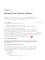
Chapter ?? Defining new types of variables or constants when the standard library does not have
what you want.
Chapter ?? Entering correlation equations with units and how we support degrees Farenheit.
Chapter ?? Defining new units of measure based on SI or other existing units.
Chapter ?? Making basic models easy to use later by adding METHODS. Defining more standard
methods and your own methods so you do not have to remember how you made the model work
yesterday, last week, last year, or in your last incarnation. Its almost automatic.
2
CHAPTER 1. STARTING POINTS
1.1.2
3
Engineering Subjects
Chapter ?? Defining a chemical mixture and physical property calculations for use in process simulation. Equilibrium thermodynamics, phases, species, and all that jazz. Adding species and
correlations to the database.
Chapter ?? Defining a simple dynamic model (initial value problem) and watching it respond. Water
level in a tank.
Chapter Writing a conditional model where which equations apply is determined by variable values
or boundary expressions.
Chapter (Ben, in progress) Defining a dynamic model with end-point conditions (boundary value
problem) using our collocation (bvp) library.
Chapter 2
Vessel Model for Beginners
You read our propaganda about the ASCEND system in which we said it was to help technical people
create hard models. We said you can tackle really large models – 100,000 equations, compiling and
solving them in minutes on a PC. We also pointed out that you can readily solve the small problems
many currently solve using a spreadsheet, only once posed you can solve them inside out, upside down
and backwards.
This sounded intriguing so you downloaded the system and installed it. Hopefully, this proved
quite straight forward. You double-clicked the ASCEND icon on your desktop and started it up for
the first time. Four windows opened up. You panicked.
Who wouldn’t?
To use this system properly requires that you learn how to use it. If you pay the price to do so and we hope it is not a large price, then we believe you will find the tools we have provided to help
you create and debug models will pay you back handsomely.
This chapter and the next two chapters (Chapter ?? and Chapter ??) are meant to be a good first
step along the path to learning how to use ASCEND. We will lead you through the steps for creating
and testing a simple model. You will also learn how to improve this model so it may be more readily
shared with others. We will present our reasons for the steps we take. We will show you all the buttons
you should push as you proceed.
We strongly suggest you put time aside and go through all three of these early chapters to introduce
yourself to ASCEND. It should take you about two to three hours. The second chapter is particularly
important if you wish to understand our approach to good modeling practices.
the problem
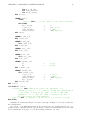
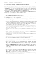
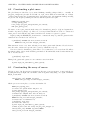
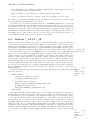
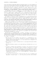
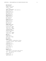
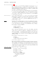
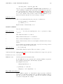
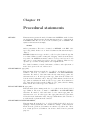
Step 1: We are going to create and test an ASCEND model to compute, the mass of the metal in
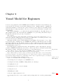
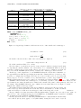
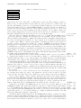
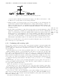
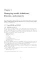
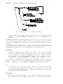
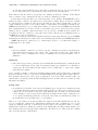
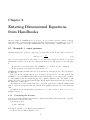
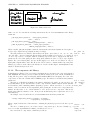
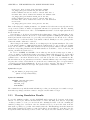
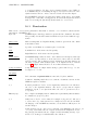
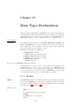
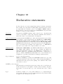
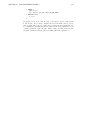
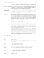
the sides and ends of the thin-walled cylindrical vessel shown in Figure ??.
Step 2: This model is to become a part of a library of models which others can use in the future.
You must document it. You must add methods to it to make it easy for others to make it well-posed.
You should probably parameterize it, and finally you must create a script which anyone can easily run
that solves an example problem to illustrate its use.
topics covered
Topics covered in this and the following two chapters are:
This chapter)
• Converting the word description to an ASCEND model.
• Loading the model into ASCEND, dealing with the error messages.
• Compiling the model.
• Browsing the model to see if it looks right
• Solving the model.
• Examining the results.
• More thoroughly testing the model.
Chapter ??
• Converting the model to a more reusable form by adding methods to it and by parameterizing
it.
4
CHAPTER 2. VESSEL MODEL FOR BEGINNERS
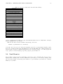
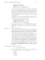
5
Figure 2.1: A thin-walled cylindrical vessel with flat ends
Symbol
D
H
wall_thickness
metal_density
Table 2.1: Variables required for model
Meaning
Typical Units
ASCEND
variable type
vessel diameter
m, ft
length
vessel height
m, ft
length
wall thickness
mm, in
length
metal density
kg/m3 , lbm/ft3
mass_density
• Creating a script to load and execute an instance of the model.
Chapter ??
• Creating an array of models.
• Using an existing library model for plotting.
• Creating a case study using the model.
We shall introduce many of the features of the modeling language as well as the use of the interactive
interface you use when compiling, debugging, solving and exploring your model. Language features
include units conversion, arrays and sets.
2.1
Converting the word description into an ASCEND model
an
ASCEND
Every ASCEND model is, in fact, a type definition. To "solve a model," we make an instance of a model is a type
type and solve the instance. So we shall start by creating a vessel type definition. We will have to definition
create our type definition as a text file using a text editor. (Some simple text editors include emacs
and gedit on Linux, and Notepad and TextPad on Windows. We shall discuss editors shortly.)
We need first to decide the parts to our model. In this case we know that we need the variables
listed in Table ??. We readily fill in the first three columns in this table. We shall discuss the entry in
the last column in a moment.
We will be computing the masses for the metal in the side wall and in the ends for this vessel. As
this is a thin-walled vessel, we shall compute the volume of metal as the area of the walls times the
wall thickness. The following equations allow us to compute the required areas
CHAPTER 2. VESSEL MODEL FOR BEGINNERS
Symbol
side_area
end_area
vessel_volume
metal_volume
metal_mass
6
Table 2.2: Some more variables required for vessel model
Meaning
Typical Units
ASCEND
variable type
area in the sidewall of
m2 , ft2
area
the vessel
total area iin the ends of
m2 , ft2
area
the vessel
volume of the vessel
m3 , ft3
volume
total volume of metal in
m3 , ft3
volume
the walls
total mass of the metal
kg, lbm
mass
in the walls of the vessel
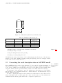
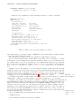
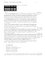
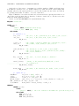
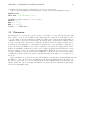
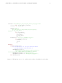
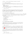
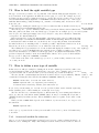
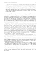
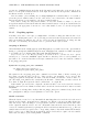
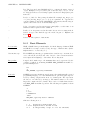
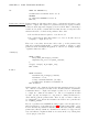
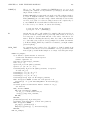
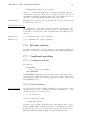
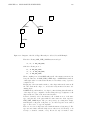
ATOM volume REFINES solver_var
DIMENSION L^3
DEFAULT 1 0 0 . 0 { f t ^3} ;
lower_bound := 0 . 0 { f t ^3} ;
upper_bound := 1 e50 { f t ^3} ;
nominal := 1 0 0 . 0 { f t ^3} ;
END volume ;
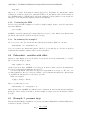
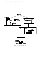
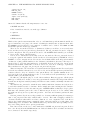
Figure 2.2: A typical type definition, called an atom, used to define variable and constant types
side wall area = πDH
πD2
4
We should be interested in the volume of the vessel, which we compute as:
single end area =
vessel volume = single end area × H
(2.1)
(2.2)
(2.3)
We add the variables in Table ?? to our list.
We believe that no one should create a model of any consequence without worrying about the units
for expressing the variables within it. We consider that to be a commandment handed down from
somewhere on high; however, we know that others do not believe as we do. Grant us our beliefs. We
have created in the ASCEND system a library of variable and constant types called atoms.a4l .
The file type ".a4l" designates it to be an ASCEND IV library file. Double-click on this link to see
the approximately 150 different types ranging from universal constants such as π (=3.14159...) and e
(=2.718...) to length, mass and angle. If we have not created one that you need, you can use this
library of types to see how to construct one for yourself and add it to your file of type definitions. You
will find detailed instructions for how to make your own variable type library in Chapter ??.
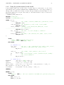
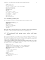
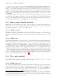
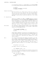
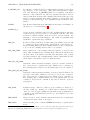
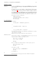
ASCEND considers variable and constant types to be elementary or "atomic" to the system. These
type definitions can contain only attributes for variables and constants. They cannot contain equations,
for example. Thus ASCEND calls such a type definition an atom rather than a model. Figure ??
illustrates the definition for the type volume.
The definition starts by stating that volume is a specialization of solver_var. The type solver_var
refines a base type in the system known as real and adds several attributes to it that a nonlinear
equation solver may need, such as a lower and upper bounds, a ’fixed’ flag, and so forth.
The type definition for volume states that volume has dimensionality of length to the power 3 (L^3)
where L is one of the 10 dimensions supported by ASCEND (see in ASCEND Syntax document for
the 10 dimensions defined within the ASCEND language).
One may express the value for a volume using any units which are consistent with the dimensionality
of L^3, such as {ft^3}, {m^3}, {gal}, or even {mile^4/mm}. Setting the lower bound to 0 {ft^3}
type definition
library for variables and constants
dimensions
and units
ASCEND.
in
CHAPTER 2. VESSEL MODEL FOR BEGINNERS
7
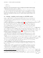
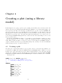
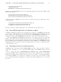
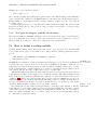
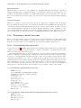
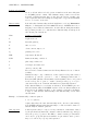
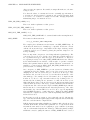
UNIVERSAL CONSTANT circle_constant
REFINES real_constant :== 1{ PI };
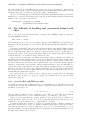
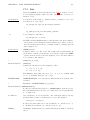
Figure 2.3: Type definition for circle_constant; has value of 1 {PI} or 3.1415927
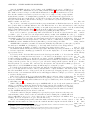
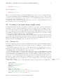
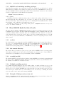
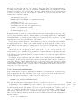
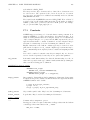
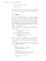
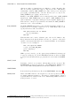
REQUIRE " atoms . a4l ";
MODEL vessel ;
(* variables *)
side_area , end_area
vessel_vol , wall_vol
wall_thickness , H , D
H_to_D_ratio
metal_density
metal_mass
IS_A
IS_A
IS_A
IS_A
IS_A
IS_A
area ;
volume ;
distance ;
factor ;
mass_density ;
mass ;
(* equations *)
FlatEnds : end_area = 1{ PI } * D ^2 / 4;
Sides : side_area = 1{ PI } * D * H ;
Cylinder : vessel_vol = end_area * H ;
Metal_volume :( side_area + 2 * end_area ) *
wall_thickness = wall_vol ;
HD_definition : D * H_to_D_ratio = H ;
VesselMass : metal_mass = metal_density * wall_vol ;
END vessel ;
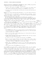
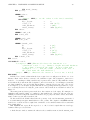
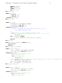
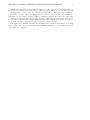
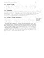
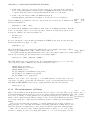
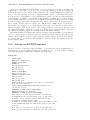
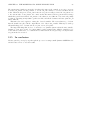
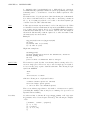
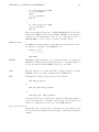
Figure 2.4: First version of the type definition for vessel.
says volume must be a nonnegative number. ASCEND used the nominal value for scaling a variable
of type volume when solving, here 100 ft3 .
One may change the values for the bounds, default and nominal values at any time.
We now can understand the last column in Table ?? and Table ??. For each variable or constant
in the system, we have identified its type in the file atoms.a4l. That is, we looked in this file for the
type definition that corresponded to the variable we were defining and listed that type here. This task
is not as onerous as it seems. As we shall see later, we provide a tool to find for you all atom types
that correspond to a particular set of units, e.g, ft^3 – i.e., the computer will do the searching for
you.
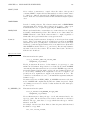
In Figure ?? we see the definition of one of the universal constants contained in atoms.a4l. This
definition is very short; it gives the name of the type circle_constant, that it refines real_constant
and that it has the value 1 {PI} where the internal conversion needed for {PI} is defined in the file
defining the built-in units in ASCEND. One can add more units if desired at any time to ASCEND
by defining one or more personal units files (Chapter ?? tells you how to do this).
universal conWe shall in fact find this constant useful in our program, and we can either introduce a constant stant definition
with this value or simply use the value 1{PI} in our program. We shall choose to do the latter.
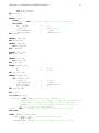
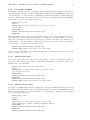
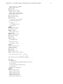
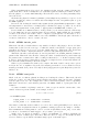
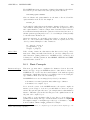
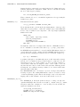
It is time to write our first version for the model, which we do in Figure ?? (available as vesselPlain.a4c
in the ASCEND model library). We first list any other files containing type definitions which this model
will use; here we list "atoms.a4l" following the keyword REQUIRE. ASCEND is sensitive to case so pay
attention to where we use and do not use capital letters. Keywords are always capitalized. Often for
clarification we use capital letters in a name we use for a variable or label (e.g., we use D for diameter
rather than d). Note that all ASCEND statements end with a semicolon (i.e., with ’;’) and not at
the end of a line and that blank lines have no impact. Comments are between opening and closing
parenthesis/asterisk pairs, i.e., ’(*’ and ’*)’.
the first version
Our model definition has the following structure for it so far:
of the code for
vessel
• MODEL statement
• list of variable we intend to use in the type definition
CHAPTER 2. VESSEL MODEL FOR BEGINNERS
8
• equations
• END statement
While we have put the statements in this order, we could mix up and intermix the middle two types
of statements, even going to the extreme of defining the variables after we first use them. The MODEL
and END statements begin and end the type definition.
You should see little that surprises you in the syntax here. However, you may have noted that we
have created a definition that says absolutely nothing about how to use the variables and equations
listed. There is no solution procedure buried in this type definition. In ASCEND the idea of solving
is separate from saying what we intend to solve. Also note that we have not said anything about the
values for any of the variables nor what we intend to calculate and what variables we intend to treat
as fixed input.
2.2
Editing, compiling and browsing an ASCEND model
Could we compile an instance of a vessel given this definition? If there had been some arrays in our
definition for which we did not say how many items were in the arrays, we could not. However, here we
could compile an instance, putting aside storage space for each of the variables and somehow capturing
the equations relating them.
When we compile new models, we need a place to store them. One possibility would be to put
them into the models subdirectory of the ASCEND installation1 . However, you really should leave
the contents of this subdirectory untouched – always. Hopefully the files will be read-only from your
user account. We count on being able to replace the model library totally every time you install a new
version of ASCEND. Whenever we add new model libraries or corrected versions of previously existing
model libraries, we put them in this subdirectory. This subdirectory belongs to us (the developers of
the system): hands off, please.
To avoid this problem, ASCEND also creates a subdirectory called ascdata that it will not touch
when you install a new version of ASCEND. It will look in this subdirectory first when looking for
a file to load when you have not given a full path name for finding that file. The install process for
ASCEND will place ascdata into your home directory??2 . ASCEND tells you where it has placed
this subdirectory when you install it. However, if you did not note where that was, then you will have
to search for it (using a tool like "FIND file or folder").
It is within the folder ascdata that you should place any ASCEND models you create. When
running a script (which we shall talk about later), ASCEND first looks in this subdirectory for files,
and then it looks in the models subdirectory. It stops looking when it finds the first available version
of the file.
Next open an editor, such as emacs, gedit, vi, vim, Notepad or TextPad. Now type in or, better
yet, cut-and-paste the statements in Figure ??. Be very careful to match the use of capital and small
letters. Do not worry about blanks between symbols but do not embed blanks within symbols. In
other words, do not put a blank in the middle of the symbol side_wall but do not worry about putting
zero or more blanks between side_wall and = in an equation.
When you are finished, be sure to save the file as a text file. Call it vesselPlain.a4c. The ".a4c"
stands for "ASCEND 4 Code". Many Windows editors will append ".txt" to the file name. Remove
the .txt ending off the file name – do not let Microsoft bully you into thinking you should not – and
change it to ".a4c".
(This model is also available as vesselPlain.a4c in the ASCEND models library, but we suggest
it would be better for you to go through the exercise of creating your own version here. At the least
copy the library file to your ASCEND space so you can play with your own version at this time.)
When you are done, you should have a text file called vesselPlain.a4c stored in your ASCEND/models/vessel subdirectory. It should contain precisely the statements in Figure ?? with care having
been taken to match capital and lower case letters as shown there.
Do not alter
the
models
subdirectory
rather put your
things into the
ascdata
subdirectory (you
own it)
create a text
file
containing the model
definition
start the AS1 On windows this might be c:\Program File\ASCEND\models. On Linux, this might be /usr/share/ascend/models. CEND system.
Move and resize
The location can vary depending on how you went about installing ASCEND.
2 On Windows, your home directory will normally be the My Documents folder. On Linux, it will normally be the windows to
/home/username . Note that in both systems, you can set an “environment” variable to designate your home directory. make
yourself
comfortable.
CHAPTER 2. VESSEL MODEL FOR BEGINNERS
9
Start the ASCEND system by double clicking on the ASCEND icon if you are on Windows or
typing ascend at the command line if you are using a Linux machine3 . Four windows will appear,
three smaller ones and one larger one that will, if left unattended, disappear by itself in a few seconds.
Move the three smaller ones around on your screen so they do not overlap or so they overlap very little.
Resize them if you want to. You might start by putting the one called Script in the upper left, the one
called Library in the upper right and the one called Console in the lower right. We shall assume you
have placed them in these positions in the following so, even if that is not your favorite placement, it
might be useful to use it for now.
As you can see, each window by itself looks like a pretty normal window. Each has buttons across
the top under which one will find different tools to run. Each also has one to three sub-windows for
displaying things. Each has a Help button that you can push at any time that you want to read all
kinds of detailed things about the window4 . For the moment we will provide you with the "just-in-time"
details here so you do not need to be sidetracked just yet by pushing these Help buttons.
If you ever lose a window, open the Script window and under the Tools button, select the window
you wish to open. You cannot lose the Script window unless you shut down ASCEND. For other
windows in ASCEND, you can close them and re-open them as required. Any window that you closed
can usually be restored by going back to the Script window and selected it from the Tools menu there.
To exit ASCEND, close the Script window. You will be asked to confirm that you want to exit
ASCEND. If you have simulations in memory this will stop you from losing your results.
ASCEND will not remember your window locations automatically. If you like where you have placed
the windows for ASCEND on your display, go to the Script window and select ’Save all appearances’
under the View menu. A similar tool exists for each window for saving only its position.
We shall start with the Library window in the upper right. This window provides you with the tools
to load and compile files containing type definitions. You can also display the code for the different
types you have loaded.
Let’s load your file. Under the File button select the ’Read types from File’ tool. You select this
tool by clicking on it using the left mouse button - i.e., the button you should have expected to use.
A window will appear asking you to find the file you want to read into ASCEND. Navigate to where
you stored vesselPlain.a4c (in the subdirectory ascdata) and select that file. If you have the wrong
ending on the file (you left .txt or you forgot to put .a4c as the ending), tell the system to list all
files and pick the one you want. The .a4c is used by the system to list only the files it thinks you
might want to load, but ASCEND isn’t fussy. It will attempt to load any file you pick.
Look in the Console window at the lower right, and, if the file loads without any errors being listed
there, you can skip past the next bit to where you should start to compile an instance. The next bit
has some useful hints on how to debug your models. If you want some debugging experience, put a
known error into your vesselPlain.a4c file and see what happens. This move will give you a reason
to read the following section.
If the Console window in the lower right starts filling with several tens of lines of diagnostics,
look to see if you included the REQUIRE statement at the beginning of your model file. Without that
statement, ASCEND is missing all the definitions for the types of variables in your model, and it will
go wild telling you so5 .
While loading the files containing these types, ASCEND will look very closely at the syntax and
will give you all kinds of diagnostic messages in the Console window (lower right) if you have done
something wrong. It will also at times spew out some warning messages if you have done something
thought to be poor modeling style. You must heed the error messages as the file will not load if there
are any. ASCEND will tell you if it did not load the file.
You should consider heeding the warnings if you get any. If you ignore them now, they may come
back and haunt you later. However, there are times when we issue a warning but everything will work,
and you will think we were not too clever. Our response: better modeling style can eliminate these
warnings. (It’s been our system so we get to have the last word.)
The error and warning messages will contain a line number in the file where the error has occurred.
This will be the line number as counted by an editor with the first line being line 1 in the file. Editors
note that each
window by itself looks pretty
nonthreatening
hey, where did
that
window
go? I want it
back NOW!
How do I quit
ASCEND?
saving window
positions
start by loading and compiling using tools
in the Library
window
use the left
mouse button
unless we tell
you otherwise
(however,
on
you own explore using the
right
mouse
button in any
of the windows)
Do not ignore
the diagnostics
that
might
appear
in
the
Console
window
how do I jump
to line 100 of
a file when
3 Depending on the Linux version you have installed, you might find that the command is ascend4 or that you have using some of
the
standard
an ASCEND option in your GNOME ’Applications’ menu.
4 assuming you have got the help files installed on your system, which you may not find you have.
editors?
5
It might also be choking on a Word document because you forgot to save it as a text file.
CHAPTER 2. VESSEL MODEL FOR BEGINNERS
10
always provide you with a means to get directly to a line number in a file. Find out how to do that or
you will not be too happy with debugging a large file.
You will be in the debug mode for a new system so do not expect it to be totally obvious the first
few times you make an error. We have tried to use language that should be meaningful, but we may
have failed or the error may be pretty subtle and not possible for us to anticipate how to describe it
in your terms. (Send us a bug report if you have any good ideas on language.)
You can reload any file your have corrected using the Read types from file tool under the File menu.
It will overwrite the previous version of the file only if the file has changed since it was last loaded
(note that we do not reload those big files unless you make a change even if you tell us to).
You can display the code you have written. Select the model vessel in the right window of the
Library. Then under the Display menu at the top, select the tool Code. The Display window will open
displaying the code for this model.
Okay, you have your file loaded without getting any diagnostics. You are ready to compile. In the
Library window, look in the left window and select the file vesselPlain.a4c. It contains the type
definition you wish to compile. You should see the type vessel appear in the right window. Select
vessel. Under the Edit button, select Create simulation. A small window opens and asks you to name
the simulation. Call it v – yes, just the letter "v", and select "OK". Short names for instances often
seem to be preferable.
Look again in the Console window for diagnostics. If everything worked without error, you will
see some statistics telling you how many models, relations and so forth you have created during the
compile step.
Select v IS A vessel in the bottom of the Library window. Then under the Export button, select
’Simulation to Browser’ to export v to the Browser tool set. The Browser window will open and
contain v. It might be useful to enlarge this window and move it down a bit, placing it a bit to the
right of the center of your screen. (Remember you can save this positioning and sizing of the Browser
window by going under the View menu and picking ’Save appearance’.)
In the left upper window of the Browser, you will find v to be the current object. Listed in the
right window are all the parts of the current object. You will see the variables listed here along with an
indication of their type. For example, you will find Cylinder IS A relation and D IS A distance
listed, among many others. Cylinder is one of the equations you wrote describing the model while D
was the diameter of the vessel.
If you pick any of the parts in the right or bottom windows, it becomes the current object; its parts
then show in the right window. For example, a relation has a boolean part (a flag that takes the value
TRUE or FALSE) indicating whether or not it is to be included when ASCEND solves the equations you
defined for the model.
If you wish to display the current value for this flag, pick ’Display Atom Values’ under the View
menu. This tool toggles a switch that causes either the value or the type to show for a variable, a
constant or a relation in the upper right window of the Browser. Try toggling it back and forth and
looking at different things in the Browser.
Pick each of the tools under View and note what happens to the displaying of things in the Browser.
Across the bottom of the Browser window note the buttons you can select labeled RV, DV and so
forth. If you have made the Browser window large enough, you will see to the right of these buttons
the type of objects whose value you want to appear or not in the lower Browser window as you toggle
each button. Toggle each of these buttons and see if the lower display changes. If it does not, then
this type of part is not in the current object.
2.3
reloading
a
file overwrites
the
previous
version
displaying the
code
now compile as
"v"
and pass the instance to the
Browser
examine v by
playing with it
in the Browser
included flags
for relations
Solving an ASCEND instance
Well, you have been patient. While there are lots of interesting tools left to explore in the Browser,
perhaps it is time to try to solve this model. To solve v, make it the current object (it alone should be
listed in the upper left window of the Browser). Then, under the Export menu, select ’to Solver’. The
Solver window will open, along with a smaller window labeled Eligible. Move the Eligible window up
a bit so it does not cover any or very little of the Solver window. Move the Solver window to the lower
left and enlarge it so you can see all of its contents.
if
ASCEND
This Eligible window is ’modal’: if it is open and you do not do something to make it happy and stops respondgo away, it will stop you from doing anything else in the ASCEND system. Such windows appear ing, hunt down
one of those
"nasty"
windows with a
"yellow
lock"
and close it
CHAPTER 2. VESSEL MODEL FOR BEGINNERS
11
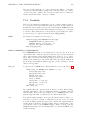
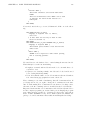
Table 2.3: Variables we have fixed
variable
D
H_to_D_ratio
meta_density
wall_thickness
with a black lock icon in a yellow field – we shall call it a "yellow lock." They demand you attend to
them now. A good solution would be for such a window to stay open and on top of all the other open
windows. Unfortunately we have not been able under all window managers to stop it from ducking
under another window. If you ever find ASCEND unwilling to respond, iconify the other windows to
get them out of the way, until you find one of these windows. On the PC you can go to the icon bar
at the bottom of your screen and, by clicking on the window, bring it to the top. Then do whatever it
takes to make it happy and close properly – such as cancel it. If you are not careful here, for example,
this window will hide under the Solver window before you are through with it.
The Solver window contains the information we need to see to explain why the Eligible window
opened in the first place. Examine the information the Solver displays. It tells you that v has 6
relations defining it and that all are equalities and included. It has no inequalities. On the right side
we see there are 10 variables and all are ’free.’ A free variable is one for which you want the system
to compute a value. Hmm, 6 equations in 10 variables. Something is wrong here. For a well-posed
problem, you want 6 equations in 6 variables (i.e., square). ASCEND reports that the system is
underspecified by 4. This means you need to pick four of the variables and declare them to be fixed.
You will also have to pick values for these fixed variables before you can solve for the remaining 6. For
such a small problem as this one, this task is not formidable. For a model with 50,000 equations and
60,000 variables, one would quit and go home. We have exposed a need here. We certainly would like
ASCEND to help us here for this small problem. But we insist that it help us in major ways to make
the 50,000 equation, 60,000 variable problem possible.
Okay, the small help such as needed here is why the Eligible window opened. Let’s return to
it. It lists all the variables of those not yet fixed that are eligible to be fixed and still leave us a
calculation that has a chance to solve. The algorithm to find eligible variables does an quick analysis
of the structure of the equations. The variables it lists are those that can be fixed without the system
becoming numerically singular. So any variables that are not shown cannot possibly help you.
So look at the list and decide what you would like to fix for your first calculation with this model.
Diameter (v.D) seems a good choice. Now you can see why we called the instance just plain old v.
A longer name would get tiring here. Anyway, pick v.D. Immediately the list reappears with v.D no
longer on it. ASCEND has just repeated the eligibility analysis, and found that more variables still
need to be fixed.
We have three more to pick. On the list are both vessel height, v.H, and v.H_to_D_ratio.
We certainly cannot pick both of these. One implies the other if we know a value for v.D. Pick
v.H_to_D_ratio. Note that v.H is no longer eligible. Good. We would be worried if it were still there.
We see v.metal_density. Pick it. Strange. Metal mass and volume stayed eligible. Why? If
we pick metal mass, wall thickness is implied, and the same is true if we were to pick metal volume.
However, as it seems much more natural to pick wall_thickness, make that the last variable you
choose. The Solver window now says this problem is square (i.e., it has 6 equations in the same
number of unknowns). Table ?? summarizes the four variables we have elected here to fix.
Toward the bottom right of the Solver window, we see there are 6 "blocks." What are blocks?
ASCEND has examined the equations and, in this case, has discovered that not all the equations have
to be solved simultaneously. There are 6 blocks of equations which it can solve in sequence. 6 blocks
and 6 equations means that ASCEND has found a way to solve the model by solving 6 individual
equations in sequence – i.e., one at a time. This is a good thing: it usually means that the solver will
have less problems with locating the overall solution.
As well as breaking down the system into blocks, ASCEND has the ability to rearrange some simple
algebraic equations so that unknown variables can be evaluated directly from the known values, with
no need for iterative numerical methods. This is only possible if there is just one equation in the block.
In fact, this problem, with the 4 variables we selected to be fixed, can be solved entirely without
is our problem
well-posed?
picking
variables we are
going to fix
ASCEND partitions
the
problem
into
smaller problems for solving
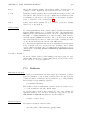
CHAPTER 2. VESSEL MODEL FOR BEGINNERS
variable
D
H_to_D_ratio
meta_density
wall_thickness
value
4
3
5000
5
12
Table 2.4: Values to use for fixed variables
units
ft
kg/m^3
mm
iteration.
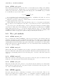
Can we see what ASCEND has just discovered? It turns out we can (we would not have asked if
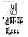
we could not). Under the Display menu on the Solver, select the ’Incidence matrix tool’. A window
pops open showing us the incidence of variables in the equations and display them in the order that
ASCEND has found to solve them, also known as a sparsity matrix or sparsity pattern. The dark
squares are incidences under the variables for which we are solving; the lighter looking ’X’ symbols to
the right side are incidences for the fixed (known) variables. Click on the incidence in the upper left
corner. ASCEND immediately identifies it for us as the end_area. It identifies the equation as the
one we labeled FlatEnds. We can go back to our model and find the equation ASCEND will solve
first. The other variable in this equation is in the set we fixed; pick it and discover it is D, the vessel
diameter. Of course we can compute the area of the ends given the diameter. The end_area is πD2 /4.
Play with the other incidences here. See what the other equations are and the order ASCEND will
use to solve them.
Okay, we return to our task of solving. We need next to supply values for the variables we have
selected to be fixed. Again, the approach we are going to take is acceptable for this small problem,
but we would not want to have to do what we are about to do for a large problem. Fortunately, we
really have thought about these issues and have some nice approaches that work even for extremely
large problem – like 100,000 equations.
Let’s see. Do you remember the variables we fixed? What if you do not? Well, we go back to the
Browser. Be sure v remains the current object (it alone is in the upper left window). Under the Find
menu select ’by Type.’ A small window opens with default information in it saying it will find for us
all objects contained in the current object v of type solver_var whose fixed flags are set to TRUE.
These are precisely the attributes for the variables we have fixed. Select OK and a list of the four
variables we fixed earlier appears.
For each variable on this list, we should supply a value. Select D in the lower window of the Browser
using the right (the right, not the left – make v the current object and do it again) mouse button. A
window opens in which we input a value for D. Put in the value 4 in the left window and ft in the right.
Continue by putting in the values for the variables as listed in Table ??. These values immediately
appear in the Browser window as you enter them. If you did not fully appreciate the proper handling
of dimension and units before, you just got a taste of its advantages. You did not have to worry about
specifying these things in consistent preselected units – ASCEND did this for you.
You can now solve this model. Go the Solver window and, under the Execute menu, select Solve.
You will get a message telling you the model solved. Dismiss that message and return to the Browser
window to examine the results. You should see the following results:
displaying
the
incidence
matrix
which variables
are
currently
fixed for this
problem?
specifying values for the fixed
variables - this
approach
is
useful for small
problems
D = 1.21922 meter
H = 3.65765 meter
H_to_D_ratio = 3
end_area = 1.16748 meter ^2
metal_density = 5000 kilogram / meter ^3
metal_mass = 408.62 kilogram
side_area = 14.0098 meter ^2
vessel_vol = 4.27025 meter ^3
wall_thickness = 0.005 meter
wall_vol = 0.0817239 meter ^3
alter the units
You may wish to alter the units used to display these results. For example, you enter the diameter used for disD in ft. You may wish to reassure yourself the 1.21922 meter is 4 ft. Go to the Script window and playing values
CHAPTER 2. VESSEL MODEL FOR BEGINNERS
13
under the Tools menu select ’Measuring units’. The Units window will open. Enlarge it appropriately
and then place it to the top and far right of your display.
There are two ways you can reset the units for displaying length.
1. Length is a basic dimension in ASCEND so under the Display button select Length. A side
window will open with all the alternate units supported in ASCEND for length. Select ft.
2. Or, in the lower part of the Units window is a frame labeled ’Set units’. Clear and then type ft
then hit Enter.
In either way, the units for all length variables will switch to ft. Look at the values in the Browser
window.
The left upper window of the Units window contains many variable types that have composite
dimensions. For example, you will find volume there. Pick it and the right window fills with all the
alternative units in which you can express volume.
Play with changing the units for displaying the various variables in the vessel instance v.
One point - the left window displaying types having composite dimensions will display only one type
for each composite dimension. If the atom types you have loaded were to include volume_difference
as well as volume, then only one of the two types, volume or volume_difference, will be listed here.
Changing the units to express either changes the units for both.
When you are done, you may wish to return to a consistent set, such as SI. Under the Display
button are different sets; pick SI (MKS) set.
We can now resolve our vessel instance in any number of different ways. For example we can ask
what the diameter would be if we had a volume of 250 ft3. To accomplish this calculation, we need
first to make vessel_volume a variable whose value we wish to fix. When we do this the model will
be overspecified. ASCEND will indicate this problem to us and offer us a list of variables - including
the vessel diameter D, one of which we will have to "unfix." Finally we need to alter the value of
vessel_volume to the desired value and solve. Explicit instructions to accomplish these steps are as
follows.
returning to a
consistent set of
units
now we can
solve the model
in other ways
• In the Browser window, make vessel_volume the current object (select it using the left mouse
button). The right window of the Browser display the parts of the vessel_volume, among them
is the fixed flag with a value of FALSE.
• (If you do not see the value for fixed but rather its type as a boolean, under the View button at
the top, select Display Atom Values.)
• Pick fixed with the right mouse button, and, in the small window that opens, delete the value
FALSE, enter the value TRUE and select OK.
• Now make v the current object by picking it in the left window of the Browser.
• Export v to the Solver again by selecting to Solver under the Export button. A window entitled
Overspecified will appear listing the variables v.D, v.H_to_D_ratio and v.vessel_volume. Pick
v.D and hit the OK button; ASCEND will reset its fixed flag to FALSE.
• Finally, return to the Browser window and select vessel_volume with the right mouse button.
In the small window that appears type 250 in the left window, ft^3 in the right, and hit the OK
button.
• Under the Execute button in the Solver window, select Solve.
Note the Solver reports only 4 blocks for 6 equations. This time it has to solve some equations
simultaneously. In the Solver window, under the Display button, select the Incidence matrix tool.
You will see that the first three equations must be solved together as a single block of equations.
clearing all the
For a more complicated model you may wish to start over on the process of selecting which variables fixed flags
are fixed. You can set the fixed flags for all the variables in a problem to FALSE all at once – without
knowing which are currently set to TRUE. In the Browser window, under the Edit button, select the
Run method tool. A window will open that displays a list of default methods that are automatically
attached to every model in ASCEND. One is called ClearAll. Pick it and hit OK. All the fixed flags
for the entire model will now be reset to FALSE. Can you think of a way to check if this is true? (Do
CHAPTER 2. VESSEL MODEL FOR BEGINNERS
14
you remember how to check which variables are currently fixed? Repeat that check and you should
find no variables are on the list.)
You might now want to play by changing what you calculate and fix.
2.4
Discussion
You have just completed the creation and solving of a very small model in ASCEND. In doing so, you
have been exposed to some interesting issues. How can we separate the concept of the model from how
we intend to solve it? How do we make a model to be well-posed – i.e., a model involving n equations
in n unknowns – so we can solve it? How should one handle the units for the variables in a modeling
system? What we have shown you here is for a small model. We still need to show you how one can
make a large model well-posed, for example. You will start to understand how one can do this in the
next chapter.
The next chapter is crucial for you to understand if you want to begin to understand how we
approach good modeling practice. Please do continue with it. As it uses the vessel model, it would, of
course, be best to continue with that chapter now.
Chapter 3
Preparing a model for reuse
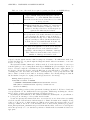
There are four major ways to prepare a model for reuse. First, you should add comments to a model.
Second, you should add methods to a model definition to pass to a future user your experience in
creating an instance of this type which is well-posed. Third, you should parameterize the model type
definition to alert a future user as to which parts of this model you deem to be the most likely to be
shared. And fourth, you should prepare a script that a future user can run to solve a sample problem
involving an instance of the model. We shall consider each of these items in turn in what follows.1
3.1
Adding comments and notes
In ASCEND we can create traditional comments for a model – i.e., add text to the code that aids
anyone looking at the code to understand what is there. We do this by enclosing text with the
delimiters (* and *). Thus the line
(* This is a comment *)
is a comment in ASCEND. Traditional comments are only visible when we display the code using the
Display code tool in the Library window or when we view the code in the text editor we used to create
it.
We suggest we can do more for the modeler with the concept of Notes, a form of "active" comments
available in ASCEND. ASCEND has tools to extract notes and display them in searchable form.
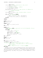
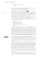
In Figure ?? we show two types of notes the modeler can add. Longer notes are set off in block
style starting with the keyword NOTES and ending with END NOTES. In this model, we declare two
notes in this manner: (1) to indicate who the author is and (2) to indicate the creation date for this
model. Note that the notes are director to documenting SELF, which is the model itself – i.e., the
vessel model as a whole object. The object one documents can be any instance in the model – any
variable, equation or part. The tools for handling notes can sort on the terms enclosed in single quotes
so one could, for example, isolate the author notes for all the models.
Vessel model with NOTES added (model vesselNotes.a4c)
REQUIRE " atoms . a 4 l " ;
MODEL v e s s e l ;
NOTES
’ a u t h o r ’ SELF { Arthur W. Westerberg }
’ c r e a t i o n ␣ d a t e ’ SELF {May , 1998 }
END NOTES;
(∗ v a r i a b l e s ∗)
side_area
" the ␣ area ␣ of ␣ the ␣ c y l i n d r i c a l ␣ s i d e ␣ wall ␣ of ␣ the ␣ v e s s e l " ,
end_area
" t h e ␣ a r e a ␣ o f ␣ t h e ␣ f l a t ␣ ends ␣ o f ␣ t h e ␣ v e s s e l "
1 More
detail on these is available in papers and reports by Allan, Zaher, Chittur et al [?],[?],[?],[?],[?].
15
CHAPTER 3. PREPARING A MODEL FOR REUSE
16
IS_A a r e a ;
vessel_vol
" t h e ␣ volume ␣ c o n t a i n e d ␣ w i t h i n ␣ t h e ␣ c y l i n d r i c a l ␣ v e s s e l " ,
wall_vol
" t h e ␣ volume ␣ o f ␣ t h e ␣ w a l l s ␣ f o r ␣ t h e ␣ v e s s e l "
IS_A volume ;
wall_thickness " the ␣ t h i c k n e s s ␣ of ␣ a l l ␣ of ␣ the ␣ v e s s e l ␣ w a l l s " ,
H
" the ␣ v e s s e l ␣ height ␣ ( of ␣ the ␣ c y l i n d r i c a l ␣ s i d e ␣ w a l l s ) " ,
D
" the ␣ v e s s e l ␣ diameter "
IS_A d i s t a n c e ;
H_to_D_ratio
" the ␣ r a t i o ␣ of ␣ v e s s e l ␣ height ␣ to ␣ diameter "
IS_A f a c t o r ;
metal_density
" d e n s i t y ␣ o f ␣ t h e ␣ metal ␣ from ␣ which ␣ t h e ␣ v e s s e l
␣␣␣␣␣␣␣␣ ␣␣␣␣␣␣␣␣ ␣␣␣␣␣␣␣␣ ␣ i s ␣ c o n s t r u c t e d "
IS_A mass_density ;
metal_mass
" t h e ␣ mass ␣ o f ␣ t h e ␣ metal ␣ i n ␣ t h e ␣ w a l l s ␣ o f ␣ t h e ␣ v e s s e l "
IS_A mass ;
(∗ equations ∗)
FlatEnds :
end_area = 1 { PI } ∗ D^2 / 4 ;
Sides :
s i d e _ a r e a = 1 { PI } ∗ D ∗ H;
Cylinder :
v e s s e l _ v o l = end_area ∗ H;
Metal_volume : ( s i d e _ a r e a + 2 ∗ end_area ) ∗ w a l l _ t h i c k n e s s = w a l l _ v o l ;
H D _d e f in i t i on : D ∗ H_to_D_ratio = H;
VesselMass :
metal_mass = m e t a l _ d e n s i t y ∗ w a l l _ v o l ;
END v e s s e l ;
ADD NOTES IN v e s s e l ;
’ d e s c r i p t i o n ’ SELF { This model r e l a t e s t h e d i m e n s i o n s o f a
c y l i n d r i c a l v e s s e l −− e . g . , diameter , h e i g h t and w a l l t h i c k n e s s
t o t h e volume o f metal i n t h e w a l l s .
It uses a thin wall
assumption −− i . e . , t h a t t h e volume o f metal i s t h e a r e a o f
the v e s s e l times the wall t h i c k n e s s . }
’ p u r p o s e ’ SELF { t o i l l u s t r a t e t h e i n s e r t i o n o f n o t e s i n t o a model }
END NOTES;
A user may use any term desired in the single quotes. We have not decided yet what the better
set of terms should be so we do not as yet suggest any. With time we expect the terms used to settle
down to just a few that are repeated for all the models in a library.
There are also short notes we can attach to every variable in the model. A "one liner" in double
quotes just following the variable name allows the automatic annotation of variables in reports.
The last few lines of Figure ?? shows adding separate notes we write using ADD NOTES IN
syntax. This object can appear before or after or in a different file from the object it describes. This
style of note writing is useful as it allows another person to add notes to a model without changing
the code for a model. Thus it allows several different sets of notes to exist for a single model, with the
choice of which to use being up to the person maintaining the model library. Finally, it allows one to
eliminate the "clutter" the documentation often adds to the code.
3.2
Adding methods
We would next like to pass along our experiences in getting this model to be well-posed – i.e., we
would like to tell future users which variables we decided to fix and which we decided to calculate.
We would also like to provide some typical values for the variables we decided to fix. ASCEND allows
us to attach any number of methods to a type definition. Methods are procedural code that we can
CHAPTER 3. PREPARING A MODEL FOR REUSE
17
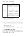
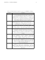
Table 3.1: Some of the methods we require for putting a model into an ASCEND library
ClearAll
specify
reset
values
a method to set all the .fixed flags for variables in the
type to FALSE. This puts these flags into a known
standard state – i.e., all are FALSE. All models inherit
this method from the base model and the need to rewrite
it is very, very rare.
a method which assumes all the fixed flags are currently
FALSE and which then sets a suitable set of fixed flags to
TRUE to make an instance of this type of model
well-posed. A well-posed model is one that is square (n
equations in n unknowns) and solvable.
a method which first runs the ClearAll method and then
the specify method. We include this method because it is
very convenient. We only have to run one method to
make any simulation well-posed, no matter how its fixed
flags are currently set. All models inherit this method
from the base model, as with ClearAll . It should only
rarely have to be rewritten for a model.
a method to establish typical values for the variables we
have fixed in an application or test model. We may also
supply values for some of the variables we will be
computing to aid in solving a model instance of this type.
These values reflectiveness that we have tested for a
simulation of this type and found to work.
request be run through the interface while browsing a model instance. We shall include methods as
described in Table ?? to set just the right fixed flags and variable values for an instance of our vessel
model to be well-posed.
The system has defaults definitions for all these methods. You already saw that to be true if you
went through the process of setting all the fixed flags to FALSE in the previous chapter. In case you
did not, load and compile the vesselPlain.a4c model in ASCEND. Export the compiled instance to
the Browser. Then in the Browser, under the Edit button, select Run method. You will see a list
containing these and other methods we shall be describing shortly. Select specify and hit the OK
button. Then look in the Console window. A message similar to the following will appear, with all
but the first line being in red to signify you should pay attention to the message:
Running method specify in v
Found STOP statement in METHOD
C:\PROGRAM FILES\ASCEND\ASCEND4\models\basemodel.a4l:307
STOP {Error! Standard method "specify" called but not
written in MODEL.};
This message is telling you that you have just run the default specify method. We have to hand-craft
every specify method so the default method is not appropriate. This message is alerting us to the fact
that we did not yet write a special specify method for this model type.
Try running the ClearAll method. The default ClearAll method is always the one you will want so
it does not put out a message to alert you that it is the default.
To write the specify and values methods for our vessel model, we note that we have successfully
solved the vessel model in at least two different ways above. Thus both variations are examples of being
‘well-posed’. We can choose which variation we shall use when creating the specify method for our
vessel type definition. Let us choose the alternative where we fixed vessel_volume, H_to_D_ratio,
metal_density and wall_thickness and provided them with the values of 250 ft^3, 3, 5000 kg/m^3
and 5 mm respectively to be our ‘standard’ specification. Default methods ClearAll and reset are
appropriate
CHAPTER 3. PREPARING A MODEL FOR REUSE
18
As already noted, the purpose of ClearAll is to set all the variables to FREE, a well-defined state
from which we can start over to set variables FIXed as we wish. The method reset simply runs
ClearAll followed by the specify method for a model. The default versions for these two methods
are generally exactly what one wants so one need not write these.
Figure ?? illustrates our vessel model with our local versions added for specify and values. Look
only at these for the moment and note that they do what we described above. We show some other
methods we shall explain in a moment.
Version of vessel with METHODS added (vesselMethods.a4c)
REQUIRE " atoms . a 4 l " ;
MODEL v e s s e l ;
NOTES
’ a u t h o r ’ SELF { Arthur W. Westerberg }
’ c r e a t i o n ␣ d a t e ’ SELF {May , 1998 }
END NOTES;
(∗ v a r i a b l e s ∗)
side_area
" the ␣ area ␣ of ␣ the ␣ c y l i n d r i c a l ␣ s i d e ␣ wall ␣ of ␣ the ␣ v e s s e l " ,
end_area
" t h e ␣ a r e a ␣ o f ␣ t h e ␣ f l a t ␣ ends ␣ o f ␣ t h e ␣ v e s s e l "
IS_A a r e a ;
vessel_vol
" t h e ␣ volume ␣ c o n t a i n e d ␣ w i t h i n ␣ t h e ␣ c y l i n d r i c a l ␣ v e s s e l " ,
wall_vol
" t h e ␣ volume ␣ o f ␣ t h e ␣ w a l l s ␣ f o r ␣ t h e ␣ v e s s e l "
IS_A volume ;
wall_thickness " the ␣ t h i c k n e s s ␣ of ␣ a l l ␣ of ␣ the ␣ v e s s e l ␣ w a l l s " ,
H
" the ␣ v e s s e l ␣ height ␣ ( of ␣ the ␣ c y l i n d r i c a l ␣ s i d e ␣ w a l l s ) " ,
D
" the ␣ v e s s e l ␣ diameter "
IS_A d i s t a n c e ;
H_to_D_ratio
" the ␣ r a t i o ␣ of ␣ v e s s e l ␣ height ␣ to ␣ diameter "
IS_A f a c t o r ;
metal_density
" d e n s i t y ␣ o f ␣ t h e ␣ metal ␣ from ␣ which ␣ t h e ␣ v e s s e l
␣␣␣␣␣␣␣␣ ␣␣␣␣␣␣␣␣ ␣␣␣␣␣␣␣␣ ␣ i s ␣ c o n s t r u c t e d "
IS_A mass_density ;
metal_mass
" t h e ␣ mass ␣ o f ␣ t h e ␣ metal ␣ i n ␣ t h e ␣ w a l l s ␣ o f ␣ t h e ␣ v e s s e l "
IS_A mass ;
(∗ equations ∗)
FlatEnds :
end_area = 1 { PI } ∗ D^2 / 4 ;
Sides :
s i d e _ a r e a = 1 { PI } ∗ D ∗ H;
Cylinder :
v e s s e l _ v o l = end_area ∗ H;
Metal_volume : ( s i d e _ a r e a + 2 ∗ end_area ) ∗ w a l l _ t h i c k n e s s = w a l l _ v o l ;
H D _d e f in i t i on : D ∗ H_to_D_ratio = H;
VesselMass :
metal_mass = m e t a l _ d e n s i t y ∗ w a l l _ v o l ;
METHODS
METHOD s p e c i f y ;
NOTES
’ p u r p o s e ’ SELF { t o f i x f o u r v a r i a b l e s and make t h e problem w e l l −posed }
END NOTES;
FIX v e s s e l _ v o l ;
FIX H_to_D_ratio ;
FIX w a l l _ t h i c k n e s s ;
CHAPTER 3. PREPARING A MODEL FOR REUSE
19
FIX m e t a l _ d e n s i t y ;
END s p e c i f y ;
METHOD v a l u e s ;
NOTES
’ p u r p o s e ’ SELF { t o s e t t h e v a l u e s f o r t h e f i x e d v a r i a b l e s }
END NOTES;
H_to_D_ratio
:=
2;
vessel_vol
:=
250 { f t ^3} ;
wall_thickness
:=
5 {mm} ;
metal_density
:=
5000 { kg /m^3} ;
END v a l u e s ;
METHOD b o u n d _ s e l f ;
END b o u n d _ s e l f ;
METHOD s c a l e _ s e l f ;
END s c a l e _ s e l f ;
METHOD d e f a u l t _ s e l f ;
D
H
H_to_D_ratio
vessel_vol
wall_thickness
metal_density
END d e f a u l t _ s e l f ;
END v e s s e l ;
:=
:=
:=
:=
:=
:=
1 {m} ;
1 {m} ;
1;
1 {m^3} ;
5 {mm} ;
5000 { kg /m^3} ;
ADD NOTES IN v e s s e l ;
’ d e s c r i p t i o n ’ SELF { This model r e l a t e s t h e d i m e n s i o n s o f a
c y l i n d r i c a l v e s s e l −− e . g . , diameter , h e i g h t and w a l l t h i c k n e s s
t o t h e volume o f metal i n t h e w a l l s .
It uses a thin wall
assumption −− i . e . , t h a t t h e volume o f metal i s t h e a r e a o f
the v e s s e l times the wall t h i c k n e s s . }
’ p u r p o s e ’ SELF { t o i l l u s t r a t e t h e i n s e r t i o n o f n o t e s i n t o a model }
END NOTES;
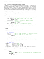
In Table ?? we describe additional methods we require before we will put a model into one of our
libraries. Each of these had two versions, both of which we require. The designation _self is for a
method to do something for all the variables and/or parts we have defined locally within the current
model with an IS_A statement. The designation _all is for a method to do something for parts that
are defined within an ‘outer’ model that has an instance of this model as a part. The ‘outer’ model
is at a higher scope. It can share its parts with this model by passing them in as parameters, a topic
we cover shortly in Section ??. Only the _self versions of these methods are relevant here and are in
Figure ??.
The bound_self and scale_self, methods we have written are both empty. We anticipate no
difficulties with variable scaling or bounding for this small model. Larger models can often give
difficult problems in solving if the variables in them are not properly scaled and bounded; these issues
must be taken very seriously for such models.
We have included the variables that define the geometry of the vessel in defaults_self method
to avoid such things as negative initial values for vessel_volume. The compiler for ASCEND runs this
method as soon as the model is compiled into an instance so the variables mentioned here start with
their default values.
Exit ASCEND and repeat all the steps above to edit, load and compile this new vessel type
definition. Then proceed as follows.
• In the Browser window, examine the values for those variables mentioned in the default_self
CHAPTER 3. PREPARING A MODEL FOR REUSE
20
Table 3.2: Additional methods required for model in ASCEND libraries
method
description
default_self,
a method called automatically when any simulation is
default_all
compiled to provide default values and adjust bounds for
any variables which may have unsuitable defaults in their
ATOM definitions. Usually the variables selected are
those for which the model becomes ill-behaved if given
poor initial guesses or bounds (e.g., zero).
bound_self,
a method to update the . upper_bound and .
bound_all
lower_bound value for each of the variables. ASCEND
solvers use these bound values to help solve the model
equations.
scale_self,
a method to update the . nominal value for each of the
scale_all
variables. ASCEND solvers will use these nominal values
to rescale the variable to have a value of about one in
magnitude to help solve the model equations.
check_self,
a method to check that the computations make sense. At
check_all
first this method may be empty, but, with experience,
one can add statements that detect answers that appear
to be wrong. As ASCEND already does bounds checking,
one should not check for going past bounds here.
However, there could be a rule of thumb available that
suggests one computed variable should be about an order
of magnitude larger than another. This check could be
done in this method.
method. Note they already have their default values.
• To place the new instance v in a solvable state, go to the Browser window. Select Run method
under the Edit menu. Select first the method values and hit OK.
• Repeat the last step but this time select the method reset.
In the Browser, examine the values for the variables listed in the method values in Figure ??. They
should be set to those stated (remember you can alter the units ASCEND uses to report the values
by using the tools in the Units window).Also examine the fixed flags for these variables; they should
all be TRUE (remember that you can find which variables are fixed all at once by using the By type
command under the Find button).
• Finally export v to the Solver. The Eligible window should NOT appear; rather that Solver
should report the model to be square.
• Solve by selecting Solve under the Execute menu.
The inclusion of methods has made the process of making this model much easier to get well-posed.
This approach is the one that works for really large, complex models.
3.3
Parameterizing the vessel model
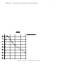
Reuse generally implies creating a model which will have as a part an instance of a previously defined
type. For example, let us compute metal_mass as a function of the H_to_D_ratio for a vessel for
a fixed vessel_volume. We would like to see if there is a value for the H_to_D_ratio for which the
metal_mass is minimum for a vessel with a given vessel_volume. We might wonder if metal_mass
goes to infinity as this ratio goes either to zero or infinity.
CHAPTER 3. PREPARING A MODEL FOR REUSE
3.3.1
21
Creating a parameterized version of vessel
To use instances of our model as parts in another model, we can parameterize it. We use parameterization to tell a future user that the parameters are objects he or she is likely to share among many
different parts of a model. We wish to create a table containing different values of H_to_D_ratio vs.
metal_mass. We can accomplish this by computing simultaneously several different vessels having the
same vessel_volume, wall_thickness and metal_density. The objects we want to see and/or share
for each instance of a vessel should include, therefore: H_to_D_ratio, metal_mass, metal_density,
vessel_volume and wall_thickness.
The code in Figure ?? indicates the changes we make to the model declaration statement and the
statements defining the variables to parameterize our model.
The parameterized version of vessel model (vesselParams.a4c)
MODEL v e s s e l (
vessel_vol
" t h e ␣ volume ␣ c o n t a i n e d ␣ w i t h i n ␣ t h e ␣ c y l i n d r i c a l ␣ v e s s e l "
WILL_BE volume ;
wall_thickness " the ␣ t h i c k n e s s ␣ of ␣ a l l ␣ of ␣ the ␣ v e s s e l ␣ w a l l s "
WILL_BE d i s t a n c e ;
metal_density
" d e n s i t y ␣ o f ␣ t h e ␣ metal ␣ from ␣ which ␣ t h e ␣ v e s s e l
␣␣␣␣␣␣␣␣ ␣␣␣␣␣␣␣␣ ␣␣␣␣␣␣␣␣ ␣ i s ␣ c o n s t r u c t e d "
WILL_BE mass_density ;
H_to_D_ratio
" the ␣ r a t i o ␣ of ␣ v e s s e l ␣ height ␣ to ␣ diameter "
WILL_BE f a c t o r ;
metal_mass
" t h e ␣ mass ␣ o f ␣ t h e ␣ metal ␣ i n ␣ t h e ␣ w a l l s ␣ o f ␣ t h e ␣ v e s s e l "
WILL_BE mass ;
);
NOTES
’ a u t h o r ’ SELF { Arthur W. Westerberg }
’ c r e a t i o n ␣ d a t e ’ SELF {May , 1998 }
END NOTES;
(∗ v a r i a b l e s ∗)
side_area
" the ␣ area ␣ of ␣ the ␣ c y l i n d r i c a l ␣ s i d e ␣ wall ␣ of ␣ the ␣ v e s s e l " ,
end_area
" t h e ␣ a r e a ␣ o f ␣ t h e ␣ f l a t ␣ ends ␣ o f ␣ t h e ␣ v e s s e l "
IS_A a r e a ;
wall_vol
H
D
" t h e ␣ volume ␣ o f ␣ t h e ␣ w a l l s ␣ f o r ␣ t h e ␣ v e s s e l "
IS_A volume ;
" the ␣ v e s s e l ␣ height ␣ ( of ␣ the ␣ c y l i n d r i c a l ␣ s i d e ␣ w a l l s ) " ,
" the ␣ v e s s e l ␣ diameter "
IS_A d i s t a n c e ;
(∗ equations ∗)
FlatEnds :
end_area = 1 { PI } ∗ D^2 / 4 ;
Sides :
s i d e _ a r e a = 1 { PI } ∗ D ∗ H;
Cylinder :
v e s s e l _ v o l = end_area ∗ H;
Metal_volume : ( s i d e _ a r e a + 2 ∗ end_area ) ∗ w a l l _ t h i c k n e s s = w a l l _ v o l ;
H D _d e f in i t i on : D ∗ H_to_D_ratio = H;
VesselMass :
metal_mass = m e t a l _ d e n s i t y ∗ w a l l _ v o l ;
METHODS
METHOD s p e c i f y ;
NOTES
’ p u r p o s e ’ SELF { t o f i x f o u r v a r i a b l e s and make t h e problem w e l l −posed }
END NOTES;
FIX v e s s e l _ v o l ;
CHAPTER 3. PREPARING A MODEL FOR REUSE
22
FIX H_to_D_ratio ;
FIX w a l l _ t h i c k n e s s ;
FIX m e t a l _ d e n s i t y ;
END s p e c i f y ;
METHOD v a l u e s ;
NOTES
’ p u r p o s e ’ SELF { t o s e t t h e v a l u e s f o r t h e f i x e d v a r i a b l e s }
END NOTES;
H_to_D_ratio
:=
2;
vessel_vol
:=
250 { f t ^3} ;
wall_thickness
:=
5 {mm} ;
metal_density
:=
5000 { kg /m^3} ;
END v a l u e s ;
METHOD b o u n d _ s e l f ;
END b o u n d _ s e l f ;
METHOD bound_all ;
RUN b o u n d _ s e l f ;
END bound_all ;
METHOD s c a l e _ s e l f ;
END s c a l e _ s e l f ;
METHOD s c a l e _ a l l ;
RUN s c a l e _ s e l f ;
END s c a l e _ a l l ;
METHOD d e f a u l t _ s e l f ;
D
H
END d e f a u l t _ s e l f ;
METHOD d e f a u l t _ a l l ;
RUN d e f a u l t _ s e l f ;
vessel_vol
wall_thickness
metal_density
H_to_D_ratio
END d e f a u l t _ a l l ;
END v e s s e l ;
:=
:=
1 {m} ;
1 {m} ;
:=
:=
:=
:=
1 {m^3} ;
5 {mm} ;
5000 { kg /m^3} ;
1;
ADD NOTES IN v e s s e l ;
’ d e s c r i p t i o n ’ SELF { This model r e l a t e s t h e d i m e n s i o n s o f a
c y l i n d r i c a l v e s s e l −− e . g . , diameter , h e i g h t and w a l l t h i c k n e s s
t o t h e volume o f metal i n t h e w a l l s .
It uses a thin wall
assumption −− i . e . , t h a t t h e volume o f metal i s t h e a r e a o f
the v e s s e l times the wall t h i c k n e s s . }
’ p u r p o s e ’ SELF { t o i l l u s t r a t e t h e i n s e r t i o n o f n o t e s i n t o a model }
END NOTES;
Substitute the statements in Figure ?? for lines 2 through 9 in Figure ??. Save the result in the
file vesselParam.a4c.
Note the use of the WILL_BE statement in the parameter list. By declaring that the type of a
parameter will be compatible with the types shown, the compiler can tell immediately if a user of this
model is passing the wrong type of object when defining an instance of a vessel.
CHAPTER 3. PREPARING A MODEL FOR REUSE
3.3.2
23
Using the parameterized vessel model
A type definition will set up our table of H_to_D_ratio values vs. metal_mass so we can observe
approximately where it attains a minimum value. ASCEND allows us to create arrays of instances of
any type. Here we shall create an array of vessels. The type definition is shown in Figure ??. Note
that the line numbers are not a part of the actual code. We include them here only so we can reference
them as needed later.
tabulated_vessel_values model
REQUIRE " atoms . a 4 l " ;
PROVIDE " v e s s e l T a b u l a t e d . a4c " ;
MODEL v e s s e l (
vessel_vol
" t h e ␣ volume ␣ c o n t a i n e d ␣ w i t h i n ␣ t h e ␣ c y l i n d r i c a l ␣ v e s s e l "
WILL_BE volume ;
wall_thickness " the ␣ t h i c k n e s s ␣ of ␣ a l l ␣ of ␣ the ␣ v e s s e l ␣ w a l l s "
WILL_BE d i s t a n c e ;
metal_density
" d e n s i t y ␣ o f ␣ t h e ␣ metal ␣ from ␣ which ␣ t h e ␣ v e s s e l
␣␣␣␣␣␣␣␣ ␣␣␣␣␣␣␣␣ ␣␣␣␣␣␣␣␣ ␣ i s ␣ c o n s t r u c t e d "
WILL_BE mass_density ;
H_to_D_ratio
" the ␣ r a t i o ␣ of ␣ v e s s e l ␣ height ␣ to ␣ diameter "
WILL_BE f a c t o r ;
metal_mass
" t h e ␣ mass ␣ o f ␣ t h e ␣ metal ␣ i n ␣ t h e ␣ w a l l s ␣ o f ␣ t h e ␣ v e s s e l "
WILL_BE mass ;
);
NOTES
’ a u t h o r ’ SELF { Arthur W. Westerberg }
’ c r e a t i o n ␣ d a t e ’ SELF {May , 1998 }
END NOTES;
(∗ v a r i a b l e s ∗)
side_area
" the ␣ area ␣ of ␣ the ␣ c y l i n d r i c a l ␣ s i d e ␣ wall ␣ of ␣ the ␣ v e s s e l " ,
end_area
" t h e ␣ a r e a ␣ o f ␣ t h e ␣ f l a t ␣ ends ␣ o f ␣ t h e ␣ v e s s e l "
IS_A a r e a ;
wall_vol
H
D
" t h e ␣ volume ␣ o f ␣ t h e ␣ w a l l s ␣ f o r ␣ t h e ␣ v e s s e l "
IS_A volume ;
" the ␣ v e s s e l ␣ height ␣ ( of ␣ the ␣ c y l i n d r i c a l ␣ s i d e ␣ w a l l s ) " ,
" the ␣ v e s s e l ␣ diameter "
IS_A d i s t a n c e ;
(∗ equations ∗)
FlatEnds :
end_area = 1 { PI } ∗ D^2 / 4 ;
Sides :
s i d e _ a r e a = 1 { PI } ∗ D ∗ H;
Cylinder :
v e s s e l _ v o l = end_area ∗ H;
Metal_volume :
( s i d e _ a r e a + 2 ∗ end_area ) ∗ w a l l _ t h i c k n e s s = w a l l _ v o l ;
H D _d e f i ni t i on : D ∗ H_to_D_ratio = H;
VesselMass :
metal_mass = m e t a l _ d e n s i t y ∗ w a l l _ v o l ;
METHODS
METHOD s p e c i f y ;
NOTES
’ p u r p o s e ’ SELF { t o f i x f o u r v a r i a b l e s and make t h e problem w e l l −posed }
END NOTES;
FIX v e s s e l _ v o l ;
FIX H_to_D_ratio ;
CHAPTER 3. PREPARING A MODEL FOR REUSE
24
FIX w a l l _ t h i c k n e s s ;
FIX m e t a l _ d e n s i t y ;
END s p e c i f y ;
METHOD v a l u e s ;
NOTES
’ p u r p o s e ’ SELF { t o s e t t h e v a l u e s f o r t h e f i x e d v a r i a b l e s }
END NOTES;
H_to_D_ratio
:=
2;
vessel_vol
:=
250 { f t ^3} ;
wall_thickness
:=
5 {mm} ;
metal_density
:=
5000 { kg /m^3} ;
END v a l u e s ;
METHOD b o u n d _ s e l f ;
END b o u n d _ s e l f ;
METHOD bound_all ;
RUN b o u n d _ s e l f ;
END bound_all ;
METHOD s c a l e _ s e l f ;
END s c a l e _ s e l f ;
METHOD s c a l e _ a l l ;
RUN s c a l e _ s e l f ;
END s c a l e _ a l l ;
METHOD d e f a u l t _ s e l f ;
D
H
END d e f a u l t _ s e l f ;
METHOD d e f a u l t _ a l l ;
RUN d e f a u l t _ s e l f ;
vessel_vol
wall_thickness
metal_density
H_to_D_ratio
END d e f a u l t _ a l l ;
:=
:=
1 {m} ;
1 {m} ;
:=
:=
:=
:=
1 {m^3} ;
5 {mm} ;
5000 { kg /m^3} ;
1;
END v e s s e l ;
ADD NOTES IN v e s s e l ;
’ d e s c r i p t i o n ’ SELF { This model r e l a t e s t h e d i m e n s i o n s o f a
c y l i n d r i c a l v e s s e l −− e . g . , diameter , h e i g h t and w a l l t h i c k n e s s
t o t h e volume o f metal i n t h e w a l l s .
It uses a thin wall
assumption −− i . e . , t h a t t h e volume o f metal i s t h e a r e a o f
the v e s s e l times the wall t h i c k n e s s . }
’ p u r p o s e ’ SELF { t o i l l u s t r a t e t h e i n s e r t i o n o f n o t e s i n t o a model }
END NOTES;
MODEL t a b u l a t e d _ v e s s e l _ v a l u e s ;
v e s s e l _ v o l u m e " volume ␣ o f ␣ a l l ␣ t h e ␣ t a b u l a t e d ␣ v e s s e l s "
IS_A volume ;
wall_thickness " t h i c k n e s s ␣ of ␣ a l l ␣ the ␣ w a l l s ␣ f o r ␣ a l l ␣ the ␣ v e s s e l s "
CHAPTER 3. PREPARING A MODEL FOR REUSE
25
IS_A d i s t a n c e ;
m e t a l _ d e n s i t y " d e n s i t y ␣ o f ␣ metal ␣ used ␣ f o r ␣ a l l ␣ v e s s e l s "
IS_A mass_density ;
n _ e n t r i e s " number␣ o f ␣ v e s s e l s ␣ t o ␣ s i m u l a t e "
IS_A integer_constant ;
n _ e n t r i e s :== 2 0 ;
H_to_D_ratio [ 1 . . n _ e n t r i e s ] " s e t ␣ o f ␣H␣ t o ␣D␣ r a t i o s ␣ f o r ␣ which ␣we␣ a r e
␣␣␣␣␣␣␣␣ ␣␣␣␣␣␣␣␣ computing ␣ metal ␣ mass "
IS_A f a c t o r ;
metal_mass [ 1 . . n _ e n t r i e s ] " mass ␣ o f ␣ metal ␣ i n ␣ w a l l s ␣ o f ␣ v e s s e l s "
IS_A mass ;
FOR i IN [ 1 . . n _ e n t r i e s ] CREATE
v [ i ] " t h e ␣ i −th ␣ v e s s e l ␣ model "
IS_A v e s s e l ( vessel_volume , w a l l _ t h i c k n e s s ,
metal_density , H_to_D_ratio [ i ] , metal_mass [ i ] ) ;
END FOR;
METHODS
METHOD d e f a u l t _ s e l f ;
END d e f a u l t _ s e l f ;
METHOD s p e c i f y ;
RUN v [ 1 . . n _ e n t r i e s ] . s p e c i f y ;
END s p e c i f y ;
METHOD v a l u e s ;
NOTES ’ p u r p o s e ’ SELF { t o s e t up 20 v e s s e l models having H t o D r a t i o s
r a n g i n g from 0 . 1 t o 2 . }
END NOTES;
v e s s e l _ v o l u m e := 250 { f t ^3} ;
w a l l _ t h i c k n e s s := 5 {mm} ;
m e t a l _ d e n s i t y := 5000 { kg /m^3} ;
FOR i IN [ 1 . . n _ e n t r i e s ] DO
H_to_D_ratio [ i ] := i / 1 0 . 0 ;
END FOR;
END v a l u e s ;
METHOD s c a l e _ s e l f ;
END s c a l e _ s e l f ;
END t a b u l a t e d _ v e s s e l _ v a l u e s ;
ADD NOTES IN t a b u l a t e d _ v e s s e l _ v a l u e s ;
’ d e s c r i p t i o n ’ SELF { This model s e t s up an a r r a y o f v e s s e l s t o
compute a r a n g e o f metal_mass v a l u e s f o r d i f f e r e n t v a l u e s
o f H_to_D_ratio . }
’ p u r p o s e ’ SELF { t o i l l u s t r a t e t h e u s e o f a r r a y s i n ASCEND}
END NOTES;
Add this model to the end of the file vesselParam.a4c (after the vessel model) and save the file
as vesselTabulated.a4c. Compile an instance of tabulated_vessel_values (call it tvv), run the
values and specify methods for it, and then solve it. You will discover that the tenth element of
the metal_mass array, corresponding to an H_to_D_ratio of 1 has the minimum value of 510.257
kilograms.
CHAPTER 3. PREPARING A MODEL FOR REUSE
3.4
26
Creating a script to demonstrate this model
The last step to make the model reusable is to create a script that anyone can easily run. Running the
model successfully will allow a user to demonstrate the use of the model and to explore an instance it
by browsing it.
ASCEND allows one to create such a script using either an editor or the tools in the Script window.
Restart the ASCEND system. You will have three windows open plus the large one which disappears
by itself in a few seconds: the Script, the Library and the Console windows.
In the Script window you will see the license agreement information for ASCEND. First clear the
license agreement from this window by doing the following two steps:
• Click Select all under the Edit menu.
• Then click Delete statements under the same button.
With the Script window now cleared of text, select Record actions under the Edit menu to start
recording the steps you are about to undertake. Then,
• In the Library window, under the Edit menu, select Delete all types. Hit Delete all on the
small window that appears.
• Load the file vesselTabulated.a4c, the file containing the model called tabulated_vessel_values.
Do this by selecting the Read types from file tool under the File menu and browsing the file system to find it. If you have trouble finding it, be sure to set the Files of type dropdown at the
bottom of the file browsing window to allow all types of files to be seen.
• Select the type tabulated_vessel_values in the right Library window and compile an instance
of it by selecting Create simulation under the Edit menu. In the small window that appears,
enter the name tvv and hit OK.
• Export the instance to the Browser by selecting Simulation to Browser under the Export
menu.
• Initialize the variable values by running the values method. Do this by selecting Run method
under the Edit menu. Select the values method and hit OK.
• Set the fixed flags to get a well-posed problem by repeating the last step but this time select
the reset method.
• Export the instance tvv to the Solver by selecting to Solver under the Export menu.
• Solve tvv by selecting Solve under the Execute menu in the Solver window.
• Return to the Script window and turn off the recording by deselecting the Record actions
option under the Edit menu.
• Save the script you have just created by selecting Save under the File menu of the Script
window. Name the file vesselTabulated.a4s (note the ’s’ ending) to indicate it is a script file
corresponding to the model file vesselTabulated.a4c (note the ’c’ ending) file.
• Exit by selecting Exit ASCEND under the File menu on the Script window. The contents of
the Script window at this point will be similar to that in Figure ?? (although the path to the
file may differ).
• Restart ASCEND.
• Open the script you just created by selecting Read file under the File menu on the Script
window. (Be sure you are allowing the system to see files with the ending .a4s by using the
Files of type dropdown at the bottom of the file-browsing window.)
• Highlight all the instructions in this script and then execute the highlighted instructions by
selecting Statements selected under the Execute menu.
CHAPTER 3. PREPARING A MODEL FOR REUSE
27
You will run the same sequence of instructions you ran to create the script.
Script to run vesselTabulated.a4c (this is the contents of the file vesselTabulated.a4s)
DELETE TYPES;
READ FILE " v e s s e l T a b u l a t e d . a4c " ;
COMPILE tvv OF t a b u l a t e d _ v e s s e l _ v a l u e s ;
BROWSE { tvv } ;
RUN { tvv . r e s e t } ;
RUN { tvv . v a l u e s } ;
SOLVE { tvv } WITH QRSlv ;
3.5
Discussion
In this chapter we converted the vessel model into a form where you and others in the future will
have a chance to reuse it. We did this by first adding methods to make the problem well-posed and
to provide values for the fixed variables for which we readily found a solution when playing with our
original model as we did in the previous chapter. We then thought of a typical use for this model and
developed a parameterized version based on that use. If this model were in a library, a future user of
it would most often simply have to understand the parameters to create an instance of this type of
model. We next added NOTES, a form of active comments, to the model. We suggest that notes are
much more useful than comments as we can provide tools that can extract them and allow us to search
them, for example, to find a model with a given functionality. Finally, we showed you how to create
a script by turning on a "phone" session where ASCEND records the actions one takes when loading,
compiling and solving a model. One can save and play this script in the future to see a typical use of
the model.
In the next chapter, we look at how we can plot the results we created in the model vesselTabulated.a4c.
We will have to reuse a model someone else has put into the library of available models. In other words,
the "shoe is on the other foot," and we quickly experience the difficulties with reuse first hand. We
will also learn how to run a case study from which we can extract the same information with a single
vessel model run multiple times.
Chapter 4
Creating a plot (using a library
model)
In this chapter we are going to produce a plot by using a model that someone else has created. We
gain two lessons: (1) you will understand first hand the difficulties one encounters when trying to use
a model someone else has created and (2) you will learn how to produce a plot in ASCEND. The
approach we take is not the one you should take if your goal is simply to produce this plot. Our goal
is pedagogical, not efficiency. In the last chapter we created an array of vessel models to produce the
data that we now about to plot. We approached this problem this way so you could see how one
creates arrays in ASCEND. Having this model, we have the data. The easiest thing we can do now it
use it to produce a plot.
We also have in ASCEND the ability to do case studies over a model instance, varying one or more
of the fixed variables for it over a range of values and capturing the values of other variables that
result. This powerful case study tool is the proper way to produce this plot as ASCEND only has to
compile one instance and solve it repeatedly rather than produce an array of models. We finish this
chapter showing you how to use this case study tool.
4.1
Creating a plot
We want a plot of metal_mass values vs. H_to_D_ratio. If we look around at the available tools,
we find there is a Plot option under the Display menu in the Browser window. While not obvious,
it turns out we can plot the arrays we produce when we include instances of type plt_plot_integer
and plt_plot_symbol in our model. We find these types in the file plot.a4l located in the ASCEND
models directory which is distributed with ASCEND. Figure ?? is shows a distilled version of that file.
The file plot.a4l
MODEL p l t m o d e l ( ) REFINES cmumodel ( ) ;
( ∗ t h e methods i n t h i s MODEL l i b r a r y have
b a s i c a l l y n o t h i n g t o do e x c e p t e x i s t .
∗)
METHODS
METHOD c h e c k _ s e l f ;
END c h e c k _ s e l f ;
METHOD s c a l e _ s e l f ;
END s c a l e _ s e l f ;
METHOD b o u n d _ s e l f ;
END b o u n d _ s e l f ;
METHOD d e f a u l t _ a l l ;
END d e f a u l t _ a l l ;
METHOD c h e c k _ a l l ;
END c h e c k _ a l l ;
28
CHAPTER 4. CREATING A PLOT (USING A LIBRARY MODEL)
29
METHOD bound_all ;
END bound_all ;
METHOD s c a l e _ a l l ;
END s c a l e _ a l l ;
END p l t m o d e l ;
MODEL p l t _ p o i n t (
x WILL_BE r e a l ;
y WILL_BE r e a l ;
) REFINES p l t m o d e l ( ) ;
END p l t _ p o i n t ;
MODEL p l t _ c u r v e (
npnts IS_A s e t OF integer_constant ;
y_data [ npnts ] WILL_BE r e a l ;
x_data [ npnts ] WILL_BE r e a l ;
)REFINES p l t m o d e l ( ) ;
( ∗ p o i n t s o f matching s u b s c r i p t w i l l be p l o t t e d i n o r d e r o f
i n c r e a s i n g subscript value .
∗)
l e g e n d " L ab el ␣ f o r ␣ c u r v e ␣ ( d i s p l a y e d ␣ i n ␣ l e g e n d ␣ box ) "
, format " c o l o u r / l i n e s t y l e ␣ i n ␣ pylab ␣ format , ␣ eg ␣ ’ r −’␣ f o r ␣ r e d ␣ l i n e "
IS_A symbol ;
FOR i IN [ npnts ] CREATE
pnt [ i ] IS_A p l t _ p o i n t ( x_data [ i ] , y_data [ i ] ) ;
END FOR;
END p l t _ c u r v e ;
ATOM p l t _ i n t e g e r _ d e f a u l t _ 0 REFINES i n t e g e r
DIMENSIONLESS
DEFAULT 0 ;
END p l t _ i n t e g e r _ d e f a u l t _ 0 ;
MODEL p l t _ p l o t _ i n t e g e r (
c u r v e _ s e t IS_A s e t OF integer_constant ;
c u r v e [ c u r v e _ s e t ] WILL_BE p l t _ c u r v e ;
)REFINES p l t m o d e l ( ) ;
t i t l e " P l o t ␣ t i t l e ␣ ( shown␣ a t ␣ top ) "
, XLabel "X−a x i s ␣ l a b e l "
, YLabel "Y−a x i s ␣ l a b e l "
IS_A symbol ;
l e g e n d _ p o s i t i o n " Legend ␣ p o s i t i o n ␣ ( s e e ␣ h t t p : / / m a t p l o t l i b . s o u r c e f o r g e . n e t / a p i / p y p l o t _ a p
IS_A p l t _ i n t e g e r _ d e f a u l t _ 0 ;
Xlow , Ylow , Xhigh , Yhigh IS_A r e a l ;
Xlog , Ylog IS_A b o o l e a n _ s t a r t _ f a l s e ;
END p l t _ p l o t _ i n t e g e r ;
MODEL plt_plot_symbol (
c u r v e _ s e t IS_A s e t OF symbol_constant ;
c u r v e [ c u r v e _ s e t ] WILL_BE p l t _ c u r v e ;
)REFINES p l t m o d e l ( ) ;
t i t l e " P l o t ␣ t i t l e ␣ ( shown␣ a t ␣ top ) "
, XLabel "X−a x i s ␣ l a b e l "
, YLabel "Y−a x i s ␣ l a b e l "
CHAPTER 4. CREATING A PLOT (USING A LIBRARY MODEL)
30
MODEL cmumodel ();
(* This MODEL does nothing except provide a root
for a collection of loosely related models .
If it happens to reveal a few bugs in the software ,
and perhaps masks others , well , what me worry ? BAA , 8/97.
*)
END cmumodel ;
Figure 4.1: The code for cmumodel
IS_A symbol ;
l e g e n d _ p o s i t i o n " Legend ␣ p o s i t i o n ␣ ( s e e ␣ h t t p : / / m a t p l o t l i b . s o u r c e f o r g e . n e t / a p i / p y p l o t _ a p
IS_A p l t _ i n t e g e r _ d e f a u l t _ 0 ;
Xlow , Ylow , Xhigh , Yhigh IS_A r e a l ;
Xlog , Ylog IS_A b o o l e a n _ s t a r t _ f a l s e ;
END plt_plot_symbol ;
As you can see, this file contains the two types we seek. However, before we can use them, we do
need to understand them. We are, so to speak, on the receiving end of the reusability issue. To make
that less painful, we will examine how the above code works. If these models were better documented,
they would be much less difficult to interpret. In time we will add Notes to them to remedy this
deficiency.
4.1.1
Model refinement
The first model, pltmodel, is two lines long, having a MODEL statement indicating it "refines" cmumodel and an END statement. We have not encountered the concept of refinement as yet. In ASCEND
the to refine means the model pltmodel inherits all the statements of cmumodel, a model which has
been defined at the end of the file system.a4l. We show the code for cmumodel in Figure ??, and we
note that it too is an empty model. It is, as it says, a root for a collection of loosely related models.
You will note (and forgive) a bit of dry humor by its author, Ben Allan. So far as we know, this model
neither provokes nor hides any bugs.
We need to introduce the concept of type refinement to understand these models. We divert for a
moment to do just that.
Suppose model B refines model A. We call A the parent model and B the child. The child model
B inherits all the code defining the parent model A. In writing the code for model B, we do not write
the code it inherits from A; we simply understand it is there already. The code we write for model
B will be only those statements that we wish to add beyond the code defining its parent. ASCEND
supports only single inheritance; thus a child may have only one parent. A parent, on the other hand,
may have many children, each inheriting its code.
We are dealing in ASCEND with models defined by their variables and equations. As we have
noted above, the order for the statements defining each of these does not matter – i.e., the variables
and equations may be defined in any order. So adding new variables and equations through refinement
may be done quite easily.
In constrast, the methods are bits of procedural code – i.e., they are run as a sequence of statements
where order does matter. In ASCEND, a child model will inherit all the methods of the parent. If
you wish to alter the code for a method, you must replace it entirely, giving it the same name as
the method to be replaced. (However, if you look into the documentation on the language syntax for
methods, you will find that the original method is still available for execution. You simply have to
add a qualifier to its name to point to it.)
If we look into this file we see the refinement hierarchy shown in Figure ??. ’cmumodel’ is the
parent model for all these models. pltmodel is its child. The remaining three models are children of
pltmodel.
There are three reasons to support model refinement, with the last being the most important one.
• We write more compact code: The first reason is compactness of coding. One can inherit a lot of
please, explain
"refines"
parents
and
children
in
a
refinement
hierarchy
order does not
matter in nonprocedural code
but it does in
the procedural
code for methods
reasons for refinement
CHAPTER 4. CREATING A PLOT (USING A LIBRARY MODEL)
31
Figure 4.2: The refinement hierarchy in the file plot.a4l
code from a parent. Only the new statements belonging to the child are then written to define
it. This is not a very important reason for having refinement.
• Changes we make to the parent propagate: A second reason is that one can edit changes into the
parent and know that the children will inherit those changes without having to alter the code
written for the child. (Of course, one can change the parent in such a way that the changes to the
child are not what is wanted for the child, introducing what will likely become some interesting
debugging problems.)
• We know what can substitute for what: The most important reason is that inheritance tells us
what kinds of parts may be substituted for a particular part in a model. Because a child inherits
all the code from its parent, we know the child has all the variables and equations defined for it
that the parent does – and typically more. We can use an instance of the child as a replacement
for an instance of the parent. Thus if you were to write a model with the part A1 of type A in it,
someone else can create an instance of your model and substitute a part B1 which is of type B.
This substituted part will have all the needed variables in it that you assumed would be there.
This third reason says that when a object passed as a parameter WILL_BE of type A, we know that a
part of either type A or type B will work.
4.1.2
Continuing with creating a plot
We are going to include in our model a part of type plt_plot_integer or plt_plot_symbol that
ASCEND can plot. We need to look at the types of parameters required by whichever of these two we
select to include here. Tracing back to its parents, we see them to be empty so all the code for these
types is right here.
The first parameter we need is a curve_set which is defined to be a set of integer_constant or
of symbol_constant. We have to guess at this time at the purpose for curve_set. It would really
help to have notes defining the intention here and to have a piece of code that would demonstrate the
use of these models. At present, we do not. We proceed, admitting we will appear to "know" more
than we should about this model. It turns out that curve_set allows us to identify each of the curves
we are going to plot. These models assume we are plotting several variables (let’s call them y[1], y[2],
...) against the same independent variable x. The values for curve_set are the ’1’, ’2’, etc. identifying
these curves.
Here we wish to plot only one curve presenting metal_mass vs. H_to_D_ratio. We can elect to
use plt_plot_symbol and label this curve ’5 mm’. The label ’5 mm’ is a symbol so we will create a
set of type symbol with this single member.
The second object has to be a object of type plt_curve.
Looking at line 45, we see how to include an object of type plt_curve. It must be passed three
objects: a set of integers (e.g., the set of integers from 1 to 20) and two lists of data giving the y-values
vs. the x-values for the curve. In the model tabulated_vessel_values, we have just these two lists, and
they are named metal_mass and H_to_D_ratio.
You need now to add to the model tabulated_vessel_values in Figure ?? (it is saved as vesselPlot.a4c). It contains a part called massVSratio of type plt_plot_symbol that ASCEND can plot.
This code is at the end of the declarative statements in tabulated_vessel_values. It also replaces the
first method, default_self.]
Also just after the first line in this file – which reads
with the most
important being we know
what can substitute
for
what
CHAPTER 4. CREATING A PLOT (USING A LIBRARY MODEL)
CurveSet " the ␣ index ␣ set ␣ for ␣ all ␣ the ␣ curves ␣ to ␣ be ␣ plotted "
IS_A set OF symbol_constant ;
CurveSet :== [ ’5 ␣ mm ’ ];
Curves [ ’5 ␣ mm ’]
" the ␣ one ␣ curve ␣ of ␣ 20 ␣ points ␣ for ␣ metal_mass ␣ \
␣ ␣ ␣ ␣ ␣ ␣ ␣ vs . ␣ H_to_D_ratio "
IS_A plt_curve (
[1.. n_entries ] ,
metal_mass ,
H_to_D_ratio
);
massVSratio " the ␣ object ␣ ASCEND ␣ can ␣ plot "
IS_A plt_plot_symbol (
CurveSet ,
Curves
);
METHODS
METHOD default_self ;
(* set the title for the plot and the labels
for the ordinate and abscissa *)
massVSratio . title :=
’ Metal ␣ mass ␣ of ␣ the ␣ walls ␣ vs ␣ H ␣ to ␣ D ␣ ratio ␣ \
␣ ␣ ␣ ␣ ␣ ␣ ␣ ␣ ␣ ␣ ␣ ␣ ␣ for ␣ a ␣ thin - walled ␣ cylindrical ␣ vessel ’;
massVSratio . XLabel := ’H ␣ to ␣ D ␣ ratio ’;
massVSratio . YLabel := ’ metal ␣ mass ␣ IN ␣ kg / m ^3 ’;
END default_self ;
Figure 4.3: The last bit of new code to include a plot in the model tabulated_vessel_values
32
CHAPTER 4. CREATING A PLOT (USING A LIBRARY MODEL)
33
REQUIRE " atoms . a4l " ;
place the instruction
REQUIRE " plot . a4l " ;
When you solve this new instance and make massSVratio the current object, you will find the Plot
option under the Display menu in the Browser window lights up and can be selected. If you do this,
you will get a plot of metal_mass vs. H_to_D_ratio. A clear minimum is apparent on this plot at
H_to_D_ratio equal to approximately one.
You should create a script to run this model just as you did for vesselTabulated.a4c in the
previous chapter. Save it as vesselPlot.a4s.
4.2
Creating a case study from a single vessel
You may think creating an array of vessels and a complex plot object just to generate a graph is either
an awful lot of work or a method which will not work for very large models. You think correctly on
both points. The plt_plot models are primarily useful for sampling values from an array of interrelated models that represent a spatially distributed system such as the pillars in a bridge or the trays
in a distillation column. You can conduct a case study, solving a single model over a range of values
for some specified variable, using the Script command STUDY.
We will step through creating a base case and a case study using the vessel model. Start by opening
a new buffer in the Script window and turning on the record button of the Scripts edit menu. In the
Library window run the Delete all types button to clear out any previous simulations. Load the vessel
model from the file vesselMethods.a4c you created in Section 3.2????.
4.2.1
The base case
Select and compile the vessel model. Give the simulation the name V. Select the simulation V in the
bottom pane of the Library window and use the right mouse button (or Alt-x b) to send the simulation
to the Browser.
In the Browser, place the mouse cursor over the upper left pane. Use the right mouse button to
run methods reset and values, then send the model to the Solver by typing Alt-x s. Move the mouse
to the Solver window and hit the F5 key to solve the model.
We now know that it takes 535.7 kg of metal to make a 250 cubic foot vessel which is twice as high
as it is broad. Suppose that now we want to know the largest volume that this amount of metal can
contain assuming the same wall thickness is required. Perhaps a skinnier or fatter vessel can hold more,
so we need to do a case study using the aspect ratio (H_to_D_ratio) as the independent variable. Use
the Browser to change V.metal_mass.fixed to TRUE, since we are using a constant amount of metal.
The solver will want you to free a variable now, so select V.vessel_vol to be freed, since volume is
what we want to study.
script recorded
Turn off the recording button on the Script window. The recording should look something like
so far
DELETE TYPES ;
READ FILE { vesselMethods . a4c } ;
COMPILE V OF vessel ;
BROWSE { V } ;
RUN { V . reset } ;
SOLVE { V } WITH QRSlv ;
ASSIGN { V . metal_mass . fixed } TRUE { } ;
# you must type the next line in the script yourself .
ASSIGN { V . vessel_vol . fixed } FALSE { } ;
The file vesselStudy.a4s was recorded in a similar manner.
CHAPTER 4. CREATING A PLOT (USING A LIBRARY MODEL)
4.2.2
34
Case study examples
The STUDY command takes a lot of arguments. Well explain them all momentarily, but should you
forget them simply enter the command STUDY without arguments in the ASCEND Console window
or xterm window to see an error message explaining the arguments and giving an example. Enter the
following command in the Script window exactly as shown except for the file name following OUTFILE.
Specify a file to be created in your ascdata directory.
STUDY {vessel_vol} \
IN {V} \
VARYING {{H_to_D_ratio} {0.1} {0.5} {0.8} {1} {1.5} {2} \
{3} {4} {8}} \
USING {QRSlv} \
OUTFILE {/usr0/ballan/ascdata/vvstudy.dat} \
ERROR STOP;
This is the simplest form of case study; the backslashes at the end of each line mean that it is all one
big statement. Select all these lines in the Script at once with the mouse and then hit F5 to execute the
study. The solver will solve all the cases and produce the output file vvstudy.dat. The quickest way to
see the result is to enter the following command in the Script, then select and execute it. (Remember
to use the name of your file and not the name shown).
ASCPLOT {/usr0/ballan/ascdata/vvstudy.dat};
ASCPLOT CLOSE; #omit if you want to see data table
You should get a graph that looks something like Figure 4-5??. The largest volume is in the neighborhood of an H_to_D_ratio of 1.
4.2.2.1
Multi-variable studies
We now have an idea where the solution is most interesting, so we can do a detailed study where we
also monitor other variables such as surface areas. Additional variables to watch can be added to the
STUDY clause of the statement.
STUDY {vessel_vol} {end_area} {side_area} \
IN {V} \
VARYING {{H_to_D_ratio} {0.5} {0.6} {0.7} {0.8) {0.9} \
{1} {1.1} {1.2} {1.3}} \
USING {QRSlv} \
OUTFILE {/usr0/ballan/ascdata/vvstudy.dat} \
ERROR STOP;
ASCPLOT {/usr0/ballan/ascdata/vvstudy.dat};
ASCPLOT CLOSE; #omit if you want to see data table
4.2.2.2
Multi-parameter studies
We can also do a multi-parameter study, for example also varying the wall thickness allowed. In general,
any number of the fixed variables can be varied in a single study, but be aware that ASCENDs relatively
simple plotting capabilities do not yet include surface or contour maps so you will need another graphic
tool to view really pretty pictures.
STUDY {vessel_vol} \
IN {V} \
VARYING \
{{H_to_D_ratio} {0.8) {0.9} {1} {1.1} {1.2} {1.3}} \
{{wall_thickness} {4 {mm}} {5 {mm}} {6 {mm}} {7 {mm}}} \
USING {QRSlv} \
OUTFILE {/usr0/ballan/ascdata/vvstudy.dat} \
ERROR STOP;
ASCPLOT {/usr0/ballan/ascdata/vvstudy.dat};
CHAPTER 4. CREATING A PLOT (USING A LIBRARY MODEL)
Figure 4.4: Study of Volume as Function of H/D
35
CHAPTER 4. CREATING A PLOT (USING A LIBRARY MODEL)
36
In this study the peak volume occurs at the same H_to_D_ratio for any wall thickness but the vessel
volume increases for thinner walls. This may be hard to see with the default graph settings, but
column 2 in rows 8-11 (H_to_D = 1.0) of the ASCPLOT data table have the largest volumes for any
given thickness in column 1. Notice that the units must be specified for the wall_thickness values in
the VARYING clause.
4.2.2.3
Plotting output with other tools
To convert the study results from the ASCPLOT format to a file more suitable for importing into a
spreadsheet, the following command does the trick. As usual, change the names to match your ascdata
directory.
asc_merge_data_files excel \
{/usr0/ballan/ascdata/vvs.txt} \
{/usr0/ballan/ascdata/vvstudy.dat}
If you prefer Matlab style text, substitute matlab for excel in the line above and change the output
name from vvs.txt to vvs.m.
4.2.3
STUDY behavior details
We now turn to the details of the STUDY statement. As we saw in Section ??, any number of variables
to be monitored can follow the STUDY keyword.
The IN clause specifies which part of a simulation is to be sent to the Solver; a small part of a much
larger model can be studied if you so desire. All the variable and parameter names that follow the
STUDY keyword and that appear in the VARYING clause must be found in this part of the simulation.
The VARYING clauses is a list of lists. Each inner list gives the name of the parameter to vary
followed by its list of values. Each possible combination of parameter values will be attempted in
multi-parameter studies. If a case fails to solve, then the study will behave according to the option set
in the ERROR clause.
The solver named in the USING clause is invoked on each case. The solver may be any of the
algebraic solvers or optimizers, but the integrators (e.g. LSODE) are not allowed.
The case data are stored in the file name which appears in the OUTFILE clause. By default, this file
is overwritten when a STUDY is started, so if you want multiple result files, use separate file names.
When the solver fails to converge or encounters an error, the STUDY can either ignore it (ERROR
IGNORE) and go on to the next case, warn you (ERROR WARN) and go on to the next case, or stop
(ERROR STOP). The ERROR option makes it possible start a case study and go to lunch. Cases which
fail to solve will not appear in the output data file.
Note that if the model is numerically ill-behaved it is possible for a case to fail when there is in
fact a solution for that combination of parameters. STUDY uses the solution of the last successfully
solved case as the initial guess for the next case, but sometimes this is not the best strategy. STUDY
also does not attempt to rescale the problem from case to case. When a case that you think should
succeed fails, go back and investigate that region of the model again manually or with a more narrowly
defined study.
4.3
Discussion
We have just led you step by step through the process of creating, debugging and solving a small
ASCEND model. We then showed you how to make this model more reusable, first by adding comments
and methods. Methods capture the "how you got it well-posed" experience you had when first solving
an instance of the vessel model. We then showed you how to parameterize this model and then use
it to construct a table of metal_mass values vs. H_to_D_ratio values. Finally we showed you how
to add a plot of these results. You should next look at the chapter in the documentation where you
create two more small ASCEND models. This chapter gives you much less detail on the buttons to
push. Finally, if you are a chemical engineer, you should look at the chapter on the script and model
for a simple flowsheet (simple_fs.a4s and simple_fs.a4c respectively).
CHAPTER 4. CREATING A PLOT (USING A LIBRARY MODEL)
37
With this experience you should be ready to write your own simple ASCEND models to solve
problems that you might now think of solving using a spreadsheet. Remember that once you have the
model debugged in ASCEND, you can solve inside out, backwards and upside down and NOT just the
way you first posed it – unlike your typical use of a spreadsheet model.
Chapter 5
Managing model definitions,
libraries, and projects
Most complex models are built from parts in one or more libraries. In this chapter we show typical
examples of how to make sure your model gets the libraries it needs. We then explain in more general
terms the ASCEND mechanism which makes this work and how you can use it to manage multiple
modeling projects simultaneously.
5.1
Using REQUIRE and PROVIDE
5.1.1
REQUIREing system.a4l
Suppose you are in a great hurry and want to create a simple model and solve it without concern for
good style, dimensional consistency, or any of the other hobgoblins we preach about elsewhere. You
will write equations using only generic_real variables as defined in system.a4l. The equations in
this example do not necessarily have a solution. In your ascdata (see howto1) directory you create an
application model definition file “myfile.a4c" which looks like:
REQUIRE "system.a4l";
MODEL quick_n_dirty;
x = y^2;
y = x + 2*z;
z = cos(x+y);
x,y,z IS_A generic_real;
(* homework problem 3, due May 21. *)
END quick_n_dirty;
The very first line REQUIRE "system.a4l"; tells ASCEND to find and load a file named system.a4l
if it has not already been loaded or provided in some other way. This REQUIRE statement must come
before the MODEL which uses the generic_real ATOM that system.a4l defines.
The REQUIRE statements in a file should all come at the beginning of the file before any other text,
including comments. This makes it very easy for other users or automated tools to determine which
files, if any, your models require.
On the ASCEND command line (in the Console window or xterm) or in the Script window, you
can then enter and execute the statement
READ FILE "myfile.a4c";
to cause system.a4l and then myfile.a4c to be loaded.
38
CHAPTER 5. MANAGING MODEL DEFINITIONS, LIBRARIES, AND PROJECTS
5.1.2
39
Chaining required files
Notice when you read myfile.a4c that ASCEND prints messages about the files being loaded. You
will see that a file basemodel.a4l is also loaded. In system.a4l you will find at the beginning the
statements
REQUIRE "basemodel.a4l";
PROVIDE "system.a4l";
The basemodel library is loaded in turn because of the REQUIRE statement in system.a4l. We will
come back to what the PROVIDE statement does in a moment. This chaining can be many files deep.
To see a more complicated example, enter
READ FILE column.a4l;
and watch the long list of files that gets loaded. If you examine the first few lines of each file in
the output list, you will see that each file REQUIRES only the next lower level of libraries. This
style minimizes redundant loading messages and makes it easy to substitute equivalent libraries in the
nested lower levels without editing too many higher level libraries. The term "equivalent libraries" is
defined better in the later section on PROVIDE.
5.1.3
Better application modeling practice
5.1.4
Substitute libraries and PROVIDE
never
require
It is generally a bad idea to create a model using only generic_real variables. The normal practice is system.a4l
in
to use correct units in equations and to use dimensional variables. In the following file we see that this an application
is done by requiring atoms.a4l instead of system.a4l and by using correct units on the coefficients model.
in the equations.
REQUIRE "atoms.a4l"; MODEL quick_n_clean;
x = y^2/1{PI*radian};
y = x + 2{PI*radian}*z;
z = cos(x+y);
x, y IS_A angle;
z IS_A dimensionless;
(* homework problem 3, due May 21. *)
END quick_n_clean;
ASCEND keeps a list of the already loaded files, as we hinted at in Section ??. A library file should
contain a PROVIDE statement, as system.a4l does, telling what library it supplies. Normally the
PROVIDE statement just repeats the file name, but this is not always the case. For example, see the
first few lines of the file ivpsystem.a4l, which include the statement
PROVIDE "system.a4l";
indicating that ivpsystem.a4l is intended to be equivalent to file system.a4l while also supplying
new features. When ivpsystem.a4l is loaded both "system.a4l" and "ivpsystem.a4l" get added to
the list of already loaded files. For one explanation of when this behavior might be desirable, see
Section ??. Another use for this behavior is when creating and testing a second library to eventually
replace the first one.
When a second library provides compatible but extended definitions similar to a first library, the
second can be substituted for the first one. The second library will obviously have a different file name,
but there is no need to load the first library if we already have the second one loaded. ivpsystem.a4l
is a second library substitutable for the first library system.a4l. Note that the reverse is not true:
system.a4l does not
PROVIDE "ivpsystem.a4l";
so system is not a valid substitute for ivpsystem.
CHAPTER 5. MANAGING MODEL DEFINITIONS, LIBRARIES, AND PROJECTS
5.1.5
40
REQUIRE and combining modeling packages
Model libraries frequently come in interrelated groups. For example, the models referred to in Ben
Allan’s thesis are published electronically as a package models/ben/ in ASCEND IV release 0.9. To
use Ben’s distillation libraries, which require rather less memory than the current set of more flexible
models, your application model should have the statement
REQUIRE "ben/bencolumn.a4l";
at the beginning.
Combining models from different packages may be tricky if the package authors have not documented them well. Since all packages are open source code that you can copy into your ascdata
directory and modify to suit your needs, the process of combining libraries usually amounts to changing the names of the conflicting model definitions in your copy.
Do NOT use \ instead of / in the package name given to a REQUIRE statement even if you are
forced to use Microsoft Windows.
5.2
How REQUIRE finds the files it loads
The file loading mechanism of REQUIRE makes it simple to manage several independent sets of models
in simultaneous development. We must explain this mechanism or the model management may seem
somewhat confusing. When a statement is processed, ASCEND checks in a number of locations for
a file with that name: ascdata, the current directory, and the ascend4/models directory. We will
describe how you can extend this list later. ASCEND also looks for model packages in each of these
same locations.
5.2.1
ascdata
If your ascdata directory exists and is readable, ASCEND looks there first for required files. Thus you
can copy one of our standard libraries from the directory ascend4/models to your ascdata directory
and modify it as you like. Your modification will be loaded instead of our standard library. The
ascdata directory is typically put into your HOME directory (see Section ??).
5.2.2
the current directory
The current directory is what you get if you type ’pwd’ at the ASCEND Console or xterm prompt.
Under Microsoft Windows, the current directory is usually some useless location. Under UNIX, the
current directory is usually the directory from which you started ASCEND.
5.2.3
ascend4/models/
The standard (CMU) models and packages distributed with ASCEND are found in the ascend4/models/
subdirectory where ASCEND is installed. This directory sits next to the directory ascend4/bin/ where
the ascend4 or ascend4.exe executable is located.
5.2.4
Multiple modeling projects
If you dislike navigating multi-level directories while working on a single modeling project, you can
separate projects by keeping all files related to your current project in one directory and changing to
that directory before starting ASCEND. If you have files that are required in all your projects, keep
those files in your ascdata directory. Under Windows, cd to the directory containing the current
project from the Console window after starting ASCEND.
5.2.5
Example: Finding ben/bencolumn.a4l
Suppose an application model requires bencolumn.a4l from package ben as shown in Section ??.
Normally ASCEND will execute this statement by searching for:
CHAPTER 5. MANAGING MODEL DEFINITIONS, LIBRARIES, AND PROJECTS
41
~/ascdata/ben/bencolumn.a4l
./ben/bencolumn.a4l
$ASCENDDIST/ascend4/models/ben/bencolumn.a4l
Assuming we started ASCEND from directory /usr1/ballan/projects/test1 under UNIX, the full
names of these might be
/usr0/ballan/ascdata/ben/bencolumn.a4l
/usr1/ballan/projects/test1/ben/bencolumn.a4l
/usr/local/lib/ascend4/models/ben/bencolumn.a4l
Assuming we started ASCEND from some shortcut on a Windows desktop, the full names of these
locations might be
C:\winnt\profiles\ballan\ascdata\ben\bencolumn.a4l
C:\Program Files\netscape\ben\bencolumn.a4l
C:\ASCEND\ascend4\models\ben\bencolumn.a4l
The first of these three which actually exists on your disk will be the file that is loaded.
5.2.6
How REQUIRE handles file and definition conflicts
Normally you simply delete all types before loading a new or revised set of ASCEND models and thus
you avoid most conflicts. When you are working with a large simulation and several smaller ones, you
may not want to delete all the types, however. We decided to make REQUIRE handle this situation and
the almost inevitable redundant REQUIRE statements that occur in the following reasonable way.
When a file is REQUIREd, ASCEND first checks the list of loaded and provided files for a name that
matches. If the name is found, then that file is checked to see if it has changed since it was loaded.
If the file has changed, then any definition that was changed is loaded in the ASCEND Library and
the new definition is used in building any subsequently compiled simulations. Old simulations remain
undisturbed and are not updated to use the new definitions since there may be conflicts that cannot
be automatically resolved.
5.2.7
Extending the list of searched directories
ASCEND uses the environment variable ASCENDLIBRARY as the list of directory paths to search for
required files. Normally you do not set this environment variable, and ASCEND works as described
above.
To see or change the value of ASCENDLIBRARY that ASCEND is using, examine ASCENDLIBRARY
in the System utilities window available from the Script Tools menu. Changes made to environment
variables in the utilities window are NOT saved. If you are clever enough to set environment variables
before running ASCEND, you can make it look anywhere you want to put your model files. Consult
your operating system guru for information on setting environment variables if you do not already
know how.
Chapter 6
Plotting data sampled from
complex models
Often you need a plot of data sampled from arbitrary locations in a model that are not naturally grouped in a single easily plotted vector. The plot.a4l library provides models (plt_curve,
plt_plot_symbol, and plt_plot_integer) that can be used with the Browser’s Display Plot button.
In this chapter we see how to create such a plot using the ASCEND statement ALIASES/IS_A to
sample data from a mechanical system of stretched springs, masses, anchors, and fingers. Creating
plots of time series data output from ASCEND’s initial value solver LSODE is discussed in Chapter ??.
Chemical engineers who can tolerate distillation models should visit the file plotcol.a4c in the
models library for more complicated examples of plotting and visit the model simple_column_profiles
in column.a4l for more complicated examples of sampling data. Reading this chapter first may be of
help in interpreting those models.
6.1
The graph we want
We want to plot the positions X1 to X3 of the connecting hooks h1, h2, and h3 in a mechanical system
as shown in Figure ??. The anchor, hooks, springs, and finger (we could replace either spring with a
block mass, also) are all separate objects which we have modeled very simply. These models are given
at the end of the chapter and can also be found (with improvements) in force1d.a4c, a model file in
the distributed ASCEND libraries.
Plotting is usually a post-solution analysis tool, so our plots should not be entangled with the basic
models or with the total mechanical system model, st. We might want to explain the system st to
someone and this could be hard to do if the code is cluttered up with plot information.
Figure 6.1: Spring test model system, st
42
CHAPTER 6. PLOTTING DATA SAMPLED FROM COMPLEX MODELS
6.2
43
Constructing a plot curve
The plot library models follow object-oriented thinking carefully, perhaps a little too carefully. A
plt_plot_integer is a plottable model built out of plt_curves which are in turn built out of arrays
of data points from the user. Constructing these data arrays is the only significant challenge in using
the plot models. Begin by building a new model with the system st as a part:
MODEL plot_spring_test;
st IS_A spring_test;
Plot_X IS_A plt_plot_integer(curve_set,curves);
END plot_spring_test;
We want to create a plt_curve from the array of hook numbers y_data[1..3] plotted against horizontal hook position x_data[1..3]. There are obvious problems with the model above: curves and
curve_set are used without being defined, and there is no mention of x_data or y_data.
Begin by using an ALIASES/IS_A statement to construct the array of positions x_data from the
variables X stored in the hooks of model st.
x_data[Xset] ALIASES (st.h1.X,st.h2.X,st.h3.X)
WHERE Xset IS_A set OF integer_constant;
This statement creates a set, Xset, indexing a new array x_data with elements collected from st.
Since the value of Xset is not specified, it becomes by default the set [1,2,3].
Now we need the hook numbers, y_data. These do not exist in st, so we create them. We will set
the numeric values of these in the default_self method. We will include method in the final model,
but do not show it here.
y_data[Xset] IS_A real;
Having both y_data and x_data, we can construct a curve from them:
X_curve IS_A plt_curve(Xset,y_data,x_data);
6.3
Constructing the array of curves
We have a curve, but the plt_plot_integer model Plot_x expects an array of curves and the set
indexing this array as input. We can make both from X_curve easily using, once again, an ALIASES/IS_A statement.
curves[curve_set] ALIASES (X_curve)
WHERE curve_set IS_A set OF integer_constant;
All the pieces are now in place, so we have the final model:
MODEL plot_spring_test;
(* create our system model and plot. *)
st IS_A spring_test;
Plot_X IS_A plt_plot_integer(curve_set,curves);
(* Gather the sampled data into an array *)
x_data[Xset] ALIASES (st.h1.X,st.h2.X,st.h3.X)
WHERE Xset IS_A set OF integer_constant;
(* Create the Y coordinates *)
y_data[Xset] IS_A real;
(* create the curve *)
X_curve IS_A plt_curve(Xset,y_data,x_data);
(* Make X_curve into the array for plt_plot_integer *)
curves[curve_set] ALIASES (X_curve) WHERE
curve_set IS_A set OF integer_constant;
CHAPTER 6. PLOTTING DATA SAMPLED FROM COMPLEX MODELS
44
METHOD default_self;
RUN st.default_self;
st.s1.L0 := 0.2{m}; (* make st more interesting *)
RUN Plot_X.default_self;
RUN X_curve.default_self;
FOR i IN Xset DO
y_data[i] := i;
END FOR;
X_curve.legend := ’meter’;
Plot_X.title := ’Hook locations’;
Plot_X.XLabel := ’location’;
Plot_X.YLabel := ’hook #’;
END default_self;
END plot_spring_test;
6.4
Resulting position plot
We can compile the plot model and obtain the graph in with the following short script.
READ FILE force1d.a4c;
COMPILE pst OF plot_spring_test;
BROWSE {pst};
RUN {pst.st.reset};
SOLVE {pst.st} WITH QRSlv;
PLOT {pst.Plot_X} ;
SHOW LAST;
We can also obtain the plot by moving to pst.Plot_X in the Browser window and then pushing the
Display→Plot button or then typing "Alt-d p". We see the hooks are positioned near 0, 230, and 370
mm. We also see that xgraph sometimes makes less than pretty graphs (Figure ??).
6.5
1-D mechanical hook, spring, mass, anchor, and finger
models
The models used in this chapter are very simple versions of masses and springs horizontally at rest,
but possibly under tension, stretched between an anchor and a finger. Only the code absolutely
necessary for this example is given here; the full code with methods and additional comments is given
in force1d.a4c, an ASCEND modeling example in the library.
These models could easily be extended to include mass, momentum, and acceleration in two or three
dimensions. Most of the methods in the force1d.a4c models are unedited from the code generated
by the ASCEND Library button Edit→Suggest method. If you improve on these models, please share
them with us and the rest of the ASCEND community.
REQUIRE "atoms.a4l";
CONSTANT spring_constant REFINES real_constant DIMENSION M/T^2;
CONSTANT position_constant REFINES real_constant DIMENSION L;
ATOM position REFINES distance DEFAULT 0{m};
END position;
MODEL hook;
F_left, F_right IS_A force;
F_left = F_right;
X IS_A position;
METHODS
METHOD default_self;
(* ATOM defaults are fine *)
END default_self;
CHAPTER 6. PLOTTING DATA SAMPLED FROM COMPLEX MODELS
Figure 6.2: Plot_X in plot_spring_test
45
CHAPTER 6. PLOTTING DATA SAMPLED FROM COMPLEX MODELS
METHOD specify;
F_right.fixed := TRUE;
END specify;
METHOD specify_float;
END specify_float;
END hook;
MODEL massless_spring(
k IS_A spring_constant;
h_left WILL_BE hook;
h_right WILL_BE hook;
) WHERE (
h_left, h_right WILL_NOT_BE_THE_SAME;
);
L0, dx IS_A distance;
h_right.X = h_left.X + L0 + dx;
F = k * dx;
h_left.F_right = F;
h_right.F_left = F;
F IS_A force;
METHODS
METHOD default_self;
dx := 1{cm};
L0 := 10{cm};
END default_self;
METHOD specify;
L0.fixed := TRUE;
RUN h_left.reset;
RUN h_right.reset;
h_left.F_right.fixed := FALSE;
h_left.X.fixed := TRUE;
END specify;
METHOD specify_float;
L0.fixed := TRUE;
RUN h_left.specify_float;
RUN h_right.specify_float;
END specify_float;
END massless_spring;
MODEL massless_block(
h_left WILL_BE hook;
h_right WILL_BE hook;
) WHERE (
h_left, h_right WILL_NOT_BE_THE_SAME;
);
width IS_A distance;
h_left.F_right = h_right.F_left;
h_right.X = h_left.X + width;
X "center of the block" IS_A position;
X = width/2 + h_left.X;
METHODS
METHOD default_self;
width := 3{cm};
END default_self;
METHOD specify;
width.fixed := TRUE;
RUN h_left.reset;
h_left.F_right.fixed := FALSE;
46
CHAPTER 6. PLOTTING DATA SAMPLED FROM COMPLEX MODELS
h_left.X.fixed := TRUE;
RUN h_right.reset;
END specify;
METHOD specify_float;
width.fixed := TRUE;
RUN h_left.specify_float;
RUN h_right.specify_float;
END specify_float;
END massless_block;
MODEL anchor(
x IS_A position_constant;
h_right WILL_BE hook;
);
h_right.X = x;
F = h_right.F_left;
F IS_A force;
METHODS
METHOD default_self;
END default_self;
METHOD specify;
RUN h_right.reset;
END specify;
METHOD specify_float;
END specify_float;
END anchor;
MODEL finger(
h1 WILL_BE hook;
);
pull IS_A force;
h1.F_right = pull;
METHODS
METHOD default_self;
pull := 3{N};
END default_self;
END finger;
MODEL finger_test;
NOTES ’ascii-picture’ SELF {
___
__
\\--O--/\/\/\/\/\/--O--|
|--O(_ \
|___|
\ \
(reference)-h1-(s1)-h2-(m1)-h3-(pinky)
}
END NOTES;
h1 IS_A hook;
s1 IS_A massless_spring(100{kg/s^2},h1,h2);
h2 IS_A hook;
m1 IS_A massless_block(h2,h3);
h3 IS_A hook;
pinky IS_A finger(h3);
METHODS
METHOD default_self;
RUN h1.default_self;
RUN h2.default_self;
RUN h3.default_self;
RUN m1.default_self;
RUN pinky.default_self;
47
CHAPTER 6. PLOTTING DATA SAMPLED FROM COMPLEX MODELS
RUN reference.default_self;
RUN s1.default_self;
END default_self;
METHOD specify;
RUN m1.specify_float;
RUN pinky.reset;
RUN reference.specify_float;
RUN s1.specify_float;
END specify;
END finger_test;
MODEL spring_test;
NOTES ’ascii-picture’ SELF {
\\--O--/\/\/\/\/\/--O--\/\/\--O(\
(reference)-h1-(s1)-h2-(s2)-h3-(pinky)
}
END NOTES;
reference IS_A anchor(0.0{m},h1);
h1 IS_A hook;
s1 IS_A massless_spring(100{kg/s^2},h1,h2);
h2 IS_A hook;
s2 IS_A massless_spring(75{kg/s^2},h2,h3);
h3 IS_A hook;
pinky IS_A finger(h3);
METHODS
METHOD default_self;
RUN h1.default_self;
RUN h2.default_self;
RUN h3.default_self;
RUN s2.default_self;
RUN pinky.default_self;
RUN reference.default_self;
RUN s1.default_self;
END default_self;
METHOD specify;
RUN pinky.reset;
RUN reference.specify_float;
RUN s1.specify_float;
RUN s2.specify_float;
END specify;
END spring_test;
REQUIRE "plot.a4l";
MODEL plot_spring_test;
(* create our model *)
st IS_A spring_test;
(* Now gather the sampled data into an array for plotting *)
x_data[Xset] ALIASES (st.h1.X,st.h2.X,st.h3.X)
WHERE Xset IS_A set OF integer_constant;
(* Now create the Y coordinates of the plot since there is no
* natural Y coordinate in our MODEL.
*)
y_data[Xset] IS_A real; (* all will be assigned to 1.0 *)
X_curve IS_A plt_curve(Xset,y_data,x_data);
(* Make X_curve into the expected array for plt_plot *)
curves[curve_set] ALIASES (X_curve) WHERE
curve_set IS_A set OF integer_constant;
Plot_X IS_A plt_plot_integer(curve_set,curves);
48
CHAPTER 6. PLOTTING DATA SAMPLED FROM COMPLEX MODELS
METHODS
METHOD default_self;
RUN st.default_self;
st.s1.L0 := 0.2{m};
RUN X_curve.default_self;
RUN Plot_X.default_self;
FOR i IN Xset DO
y_data[i] := i;
END FOR;
X_curve.legend := ’meter’;
Plot_X.title := ’Hook locations’;
Plot_X.XLabel := ’location {m}’;
Plot_X.YLabel := ’hook #’;
END default_self;
END plot_spring_test;
49
Chapter 7
Defining Variables and Scaling
Values
the purpose of
By now you have probably read Chapter ?? and seen an example of how to create a model using existing this chapter
variable types in ASCEND. You found that variables of types area, length, mass, mass_density, and
volume were needed and that they could be found in the library atoms.a4l. You want to know how
to generalize on that; how to use variables, constants, and scaling values in your own models so that
the models will be easier to solve.
This chapter is meant to explain the following things:
• The "Big Picture" of how variables, constants, and scaling values relate to the rest of the ASCEND
IV language and to equations in particular. We’ll keep it simple here. More precise explanations
for the language purist can be found in our syntax document **syntax.fm5**. You do not need
to read about the "Big Picture" in order to read and use the other parts of this chapter, but you
may find it helpful if you are having trouble writing an equation so that ASCEND will accept it.
• How to find the type of variable (or constant) you want. We keep a mess of interesting ATOM
and CONSTANT definitions in atoms.a4l. We provide tools to search in already loaded libraries
to locate the type you need.
• How to define a new type of variable when we do not have a predefined ATOM or CONSTANT that
suits your needs. It is very easy to define your own variable types by copying code into an atoms
library of your own from atoms.a4l and then editing the copied definition.
• How to define a scaling variable to make your equations much easier to solve.
7.1
The Big Picture: a taxonomy
As you read in Chapter ??, simulations are built from MODEL and ATOM definitions, and MODEL
and ATOM definitions are defined by creating types in an ASCEND language text file that you load
into the ASCEND system. Figure ?? shows the types of objects that can be defined. You can see
there are many more types than simply real variables used for writing equations. Some of these types
can also be used in equations. You also see that there are three kinds of equations, not simply real
relations. Throughout our documentation we call real relations simply "relations" because that is the
kind of equation most people are interested in most of the time. Notice that "scaling values" do not
appear in this diagram. We will cover scaling values at the end of this The major features of this
diagram are:
ATOM
• Any variable quantity for use in relations, logical relations, or when statements or other computations. These come in the usual programming language flavors real, boolean, symbol, integer.
Not all kinds of atoms can be used in all kinds of equations, as we shall explain when describing
50
CHAPTER 7. DEFINING VARIABLES AND SCALING VALUES
51
Figure 7.1: The big picture: how to think about variables
relations in a little bit. Atoms may be assigned values many times interactively, with the Script
ASSIGN statement, with the METHOD := assignment operator, or by an ASCEND client such
as a solver.
An ATOM may have attributes other than its value, such as .fixed in solver_var, but these attributes
are not atoms. They are subatomic particles and cannot be used in equations. These attributes are
interpretable by ASCEND clients, and assignable by the user in the same ways that the user assigns
atom values.
Each subatomic particle instance belongs to exactly one atom instance (one variable in your compiled simulation). This contrasts with an atom instance which can be shared among several models
by passing the atom instance from one model into another or by creating aliases for it.
CONSTANT
• Constants are "variables" that can be assigned no more than once. By convention, all constant
types in atoms.a4l have names that end in _constant so that they are not easily confused with
atoms. A constant gets a values from the DEFAULT portion of its type definition, by an interactive assignment, or by an assignment in the a model which uses the :== assignment operator.
Constants cannot be assigned in a METHOD, nor can they be assigned with the := operator.
Integer and symbol constants can appear as members of sets or as subscripts of arrays. Integer, boolean,
and symbol constants can be used to control SELECT statements which determine your simulation’s
structure at compile-time or to control SWITCH and WHEN behavior during problem solving .
set
• Sets are unordered lists of either integer or symbol constants. A set is assigned its value exactly
once. The user interface always presents a set in sorted order, but this is for convenience only.
Sets are useful for defining an array range or for writing indexed relations. More about sets and
their use can be found in **syntax.fm5**.
relationships
• Relations and logical relations allow you to state equalities and inequalities among the variables
and constants in you models. WHEN statements allow you to state relationships among the
CHAPTER 7. DEFINING VARIABLES AND SCALING VALUES
52
models and equations which depend on the values of variables in those models. Sets and symbols
are not allowed in real or logical relations except when used as array subscripts.
Real relations relate the values of real atoms, real constants, and integer constants. Real relations
cannot contain boolean constants and atoms, nor can they contain integer atoms.
Logical relations relate the values of boolean atoms and boolean constants. The SATISFIED operator
makes it possible to include real relations in a logical relation. Neither integer atoms and constants
nor real atoms and constants are allowed in logical relations. If you find yourself trying to write an
equation with integer atoms, you are really creating a conditional model for which you should use the
WHEN statement instead. See **conditional modeling** to learn about how ASCEND represents this
kind of mathematical model. There are also a real variable types, solver_integer and solver_binary,
which are used to formulate equations when the solver is expected to initially treat the variable as a
real value but drive it to an integer or 0-1 value at the solution. The integer programming features of
ASCEND are described **elsewhere**.
Like atoms, real and logical relations may have attributes, subatomic particles for use by ASCEND
clients and users. The name of a relation can be used in writing logical relations and WHEN statements.
WHEN statements are outside the scope of this chapter; please see **conditional modeling** or
**syntax.fm5** for the details.
MODEL
• A model is simply a container for a collection of atoms, constants, sets, relations, logical relations,
when statements, and arrays of any of these. The container also specifies some of the methods
that can be used to manipulate its contents. Compiling a model creates an instance of it– a
simulation.
SOLVER_VAR
• The real atom type solver_var is the type from which all real variables that you want the system
to solve for must spring. If you define a real variable using a type which is not a refinement of
solver_var, all solvers will treat that variable as an a scaling value or other given constant
rather than as a variable.
Solver_vars have a number of subatomic attributes (upper_bound, lower_bound, and so forth) that
help solvers find the solution of your model. ATOM definitions specify appropriate default values for
these attributes that depend on the expected applications of the atom. These attribute values can
(and should) be modified by methods in the final application model where the most accurate problem
information is available.
Scaling value
• A real that is not a member of the solver_var family is ignored by the solver. Numerical solvers
for problems with many equations in many variables work better if the error computed for each
equation (before the system is solved) is of approximately size 1.0. This is most critical when
you are starting to solve a new problem at values far, far away from the solution. When the error
of one equation is much larger than the errors in the others, that error will skew the behavior of
most numerical solvers and will cause poor performance.
This is one of the many reasons that scientists and engineers work with dimensionless models: the
process of scaling the equations into dimensionless form has the effect of making the error of each
equation roughly the same size even far away from the solution. It is sometimes easiest to obtain a
dimensionless equation by writing the equation in its dimensional form using natural variables and
then dividing both sides by an appropriate scaling value. We will see how to define an atom for scaling
purposes in the last part of this chapter.
CHAPTER 7. DEFINING VARIABLES AND SCALING VALUES
7.2
53
How to find the right variable type
The type of real atom you want to use depends first on the dimensionality (length, mass/time, etc.)
needed and then on the application in which the atom is going to be used. For example, if you are
modeling a moving car and you want an atom type to describe the car’s speed, then you need to find
an atom with dimensionality length/time or in ASCEND terms L/T. There may be two or three types
with this dimensionality, possibly including real_constants, a real scaling value, and an atom derived
from solver_var.
The first step to finding the variable type needed is to make sure that atoms.a4l is loaded in your
Library window from ascend4/models/atoms.a4l.
The next step is to open the "ATOM by units" dialog found in the Library window’s Find menu.
This dialog asks for the units of the real variable type you want. For our example, speed, you would
enter "feet/second," "furlongs/fortnight," "meter^3/second/ft^2" or any other combination of units that
corresponds to the dimensionality L/T.
If the system is able to deduce the dimensionality of the units you have entered, it will return a list
of all the currently loaded ATOM and CONSTANT definitions with matching dimensions. It may fail
to understand the units, in which case you should try the corresponding SI units. If it understands
the units but there are no matching atoms or constants, you will be duly informed. If there is no atom
that meets your needs, you should create one as outlined in **the next section**.
The resulting list of types includes a Code button which will display the definition of any of the
types listed once you select (highlight) that type with the mouse. Usually you will need to examine
several of the alternatives to see which one is most appropriate to the physics and mathematics of your
problem. Compare the default, bounds, and nominal values defined to those you need. Check whether
the type you are looking at is a CONSTANT or an ATOM.
You now know the name of the variable type you need, or you know that you must create a new
one to suit your needs.
7.3
Load atoms.a4l
Find an ATOM
or CONSTANT
by units
Selecting
right type
the
How to define a new type of variable
In this section we will give examples of defining the atom and constant types as well as outline a few
exceptional situations when you should NOT define a new type. More examples can be found and
copied from atoms.a4l. You should define your new atoms in your personal atoms library.
Saving
cusThe user data file ~\ascdata\myatoms.a4l is the normal location for a personallibrary. This file tomized varicontains the following three lines and then the ATOM and CONSTANT definitions you create.
able types
REQUIRE "atoms.a4l"; (* loads our atoms first *)
PROVIDE "myatoms.a4l"; (* registers your library *)
(* Custom atoms created by <insert your name here> *)
If you develop an interesting set of atoms for some problem domain outside chemical engineering
thermodynamics, please consider mailing it to us through our web page.
The user data directory ~/ascdata may have a different name if you are running under Windows
and do not have the environment variable HOME defined. It may be something like C:\ascdata or
\WINNT\Profiles\Your Name\ascdata. When ASCEND is started, it prints out the name of this
directory.
When you write a MODEL which depends on the definition of your new atoms, do not forget to add
the statement
REQUIRE "myatoms.a4l";
at the very top of your model file so that your atoms will be loaded before your model definitions try
to use them.
7.3.1
A new real variable for solver use
Suppose you need an atom with units {dollar/ft^2/year} for some equation relating amortized construction costs to building size. Maybe this example is a bit far fetched, but it is a safe bet that our
CHAPTER 7. DEFINING VARIABLES AND SCALING VALUES
54
library is not going to have an atom or a constant for these units. Here is the standard incantation
for defining a new variable type based on solver_var. ASCEND allows a few permutations on this
incantation, but they are of no practical value. The parts of this incantation that are in italics should
be changed to match your needs. You can skip the comments, but you must include the units of the
default on the bounds and nominal.
ATOM amortized_area_cost
REFINES solver_var DEFAULT 3.0 {dollar/ft^2/year};
lower_bound := 0 {dollar/ft^2/year};
(* minimum value *)
upper_bound := 10000 {dollar/ft^2/year};
(* maximum value for any sane application *)
nominal := 10 {dollar/ft^2/year};
(* expected size for all reasonable applications*)
END amortized_area_cost;
In picking the name of your atom, remember that names should be as self-explanatory as possible. Also
avoid choosing a name that ends in _constant (as this is conventionally applied only to CONSTANT
definitions) or _parameter. Parameter is an extremely ambiguous and therefore useless word. Also
remember that the role a variable plays in solving a set of equations depends on how the solver being
applied interprets .fixed and other attributes of the variable.
Exceptions
If an atom type matches all but one of the attributes you need for your problem, say for example
the upper_bound is way too high, use the existing variable type and reassign the bound to a more
sensible value in the default_self method of the model where the variable is created. Having a dozen
atoms defined for the same units gets confusing in short order to anyone you might share your models
with.
The exception to the exception (yes, there always seems to be one of those) is the case of a
lower_bound set at zero. Usually a lower_bound of zero indicates that there is something inherently
positive about variables of that type. Variables with a bound of this type should not have these physical
bounds expanded in an application. Another example of this type of bound is the upper_bound 1.0
on the type fraction.
For example, negative temperature just is not sensible for most physical systems. ASCEND defines
a temperature atom for use in equations involving the absolute temperature. On the other hand, a
temperature difference, delta T, is frequently negative so a separate atom is defined. Anyone receiving
a model written using the two types of atoms, which both have units of {Kelvin}, can easily tell which
variables might legitimately take on negative values by noting whether the variable is defined as a
temperature or a delta_temperature.
7.3.2
A new real constant type
Real constants which do not have a default value are usually needed only in libraries of reusable models,
such as components.a4l, where the values depend on the end-user’s selection from alternatives in a
database. The standard incantation to define a new real constant type is:
CONSTANT critical_pressure_constant
REFINES real_constant DIMENSION M/L/T^2 ;
Here again, the italic parts of this incantation should be redefined for your purpose.
It is wasteful to define a CONSTANT type and a compiled object to represent a universal constant.
For example, the thermodynamic gas constant, R = 8.314... {J/mole/K}, is frequently needed in
modeling chemical systems. The SI value of R does not vary with its application. Neither does the
value of π. Numeric constants of this sort are better represented as a numeric coefficient and an
appropriately defined unit conversion. Consider the ideal gas law, PV = NRT and the ASCEND
unit conversion {GAS_C} which appears in the library ascend4/models/measures.a4l. This equation
should be written:
P * V = n * 1.0{GAS_C} * T;
Universal
exceptions
and
unit
conversions
CHAPTER 7. DEFINING VARIABLES AND SCALING VALUES
55
Similarly, area = pi*r^2 should be written
area = 1{PI} * r^2;
The coefficient 1 of {GAS_C} and {PI} in these equations takes of the dimensionality of and is multiplied
by the conversion factor implied by the UNITS definition for the units. If we check measures.a4l, we
find the definition of PI is simply {3.14159...} and the definition of GAS_C is {8.314... J/mole/K} as
we ought to expect.
For historical reasons there are a few universal constant definitions in atoms.a4l. New modelers
should not use them; they are only provided to support outdated models that no one has yet taken
the time to update.
7.3.3
New types for integers, symbols, and booleans
The syntax for ATOM and CONSTANT definitions of the non-real types is the same as for real number
types, except that units are not involved. Take your best guess based on the examples above, and you
will get it right. If even that is too hard, more details are given in **syntax.fm5**.
7.4
How to define a scaling variable
A scaling variable ATOM is defined with a name that ends in _scale as follows. Note that this ATOM
does not refine solver_var, so solvers will not try to change variables of this type during the solution
process.
ATOM distance_scale REFINES real DEFAULT 1.0{meter};
END distance_scale;
ASCEND uses a combination of symbolic and numerical techniques to create and solve mathematical
problems. Once you get the problem close to the solution, ASCEND can internally compute its own
scaling values for relations, known elsewhere as "relation nominals,” assuming you have set good values
for the .nominal attribute of all the variables. It does this by computing the largest additive term in
each equation. The absolute value of this term is a very good scaling value.
This internal scaling works quite well, but not when the problem is very far away from the solution
so that the largest additive terms computed are not at all representative of the physical situation being
modeled. The scale_self method, which should be written for every model as described in Section ??
of Chapter ?? should set the equation scaling values you have defined in a MODEL based on the best
available information. In a chemical engineering flowsheeting problem, for example, information about
a key process material flow should be propagated throughout the process flowsheet to scale all the
other flows, material balance equations, and energy balance equations.
The default value for any scaling atom should always be 1.0 in appropriate SI units, so that the
scaling will have no effect until you assign a problem specific value. Multiplying or dividing both sides
of an equation by 1.0 obviously will not change the mathematical behavior, but you do not want to
change the behavior arbitrarily either– you want to change it based on problem information that is
not contained in your myatoms.a4l file.
ASCEND cannot do it all for
you
Scaling
atom
default value
Chapter 8
Entering Dimensional Equations
from Handbooks
Often in creating an ASCEND model one needs to enter a correlation given in a handbook that is
written in terms of variables expressed in specific units. In this chapter, we examine how to do this
easily and correctly in a system like ASCEND where all equations must be dimensionally correct.
8.1
Example 1– vapor pressure
Our first example is the equation to express vapor pressure using an Antoine-like equation of the form:
ln(Psat ) = A −
B
T +C
(8.1)
where Psat is in {atm} and T in {R}. When one encounters this equation in a handbook, one then
finds tabulated values for A, B and C for different chemical species. The question we are addressing
is:
How should one enter this equation into ASCEND so one can then enter the constants A,
B, and C with the exact values given in the handbook?
ASCEND uses SI units internally. Therefore, P would have the units {kg/m/s^2}, and T would have
the units {K}.
Eqn ?? is, in fact, dimensionally incorrect as written. We know how to use this equation, but
ASCEND does not as ASCEND requires that we write dimensionally correct equations. For one thing,
we can legitimately take the natural log (ln) only of unitless quantities. Also, the handbook will
tabulate the values for A, B and C without units. If A is dimensionless, then B and C would require
the dimensions of temperature.
The mindset we describe in this chapter is to enter such equations is to make all quantities that
must be expressed in particular units into dimensionless quantities that have the correct numerical
value.
We illustrate in the following subsections just how to do this conversion. It proves to be very
straight forward to do.
8.1.1
Converting the ln term
Convert the quantity within the ln() term into a dimensionless number that has the value of pressure
when pressure is expressed in {atm}.
Very simply, we write
P_atm = P/1{atm};
Note that P_atm has to be a dimensionless quantity here.
We then rewrite the LHS of Equation ?? as
56
CHAPTER 8. ENTERING DIMENSIONAL EQUATIONS FROM HANDBOOKS
57
ln(P_atm)
Suppose P = 2 {atm}. In SI units P= 202,650 {kg/m/s^2}. In SI units, the dimensional constant
1{atm} is about 101,325 {kg/m/s^2}. Using this definition, P_atm has the value 2 and is dimensionless. ASCEND will not complain with P_atm as the argument of the ln () function, as it can take the
natural log of the dimensionless quantity 2 without any difficulty.
8.1.2
Converting the RHS
We next convert the RHS of Equation ??, and it is equally as simple. Again, convert the temperature
used in the RHS into:
T_R = T/1{R};
ASCEND converts the dimensional constant 1{R} into 0.55555555...{K}. Thus T_R is dimensionless
but has the value that T would have if expressed in {R}.
8.1.3
In summary for example 1
We do not need to introduce the intermediate dimensionless variables. Rather we can write:
ln(P/1{atm}) = A - B/(T/1{R} + C);
as a correct form for the dimensional equation. When we do it in this way, we can enter A, B and C
as dimensionless quantities with the values exactly as tabulated.
8.2
Fahrenheit– variables with offset
What if we write Equation ?? but the handbook says that T is in degrees Fahrenheit, i.e., in {F}?
The conversion from {K} to {F} is
T{F} = T{K}*1.8 - 459.67
and the 459.67 is an offset. ASCEND does not support an offset for units conversion. We shall discuss
the reasons for this apparent limitation in Section ??.
You can readily handle temperatures in {F} if you again think as we did above. The rule, even
for units requiring an offset for conversion, remains: convert a dimensional variable into dimensionless
one such that the dimensionless one has the proper value.
Define a new variable
T_degF = T/1{R} - 459.67;
Then code ??Equation 7.1 as
ln(P/1{atm}) = A - B/(T_degF + C);
when entering it into ASCEND. You will then enter constants A, B, and C as dimensionless quantities
having the values exactly as tabulated. In this example we must create the intermediate variable
T_degF.
8.3
Example 3– pressure drop
From the Chemical Engineering Handbook by Perry and Chilton, Fifth Edition, McGraw-Hill, p10-33,
we find the following correlation:
∆Pa0 =
y (Vg − Vl )G2
144g
CHAPTER 8. ENTERING DIMENSIONAL EQUATIONS FROM HANDBOOKS
58
where the pressure drop on the LHS is in psi, y is the fraction vapor by weight (i.e., dimensionless),
Vg and Vl are the specific volumes of gas and liquid respectively in ft3/lbm, G is the mass velocity in
lbm/hr/ft2 and g is the acceleration by gravity and equal to 4.18x108 ft/hr2.
We proceed by making each term dimensionless and with the right numerical value for the units in
which it is to be expressed. The following is the result. We do this by simply dividing each dimensional
variable by the correct unit conversion factor.
delPa/1{psi} = y*(Vg-Vl)/1{ft^3/lbm}*
(G/1{lbm/hr/ft^2})^2/(144*4.18e8);
8.4
The difficulty of handling unit conversions defined with
offset
How do you convert temperature from Kelvin to centigrade? The ASCEND compiler encounters the
following ASCEND statement:
d1T1 = d1T2 + a.Td[4];
and d1T1 is supposed to be reported in centigrade. We know that ASCEND stores termperatures in
Kelvin {K}. We also know that one converts {K} to {C} with the following relationshipT{C} = T{K}
- 273.15.
Now suppose d1T2 has the value 173.15 {K} and a.Td{4} has the value 500 {K}. What is d1T1 in
{C}? It would appear to have the value 173.15+500-273.15 = 400 {C}. But what if the three variables
here are really temperature differences? Then the conversion should be T{dC} = T{dK}, where we
use the notation {dC} to be the units for temperature difference in centigrade and {dK} for differences
in Kelvin. Then the correct answer is 173.15+500=673.15 {dC}.
Suppose d1T1 is a temperature and d1T2 is a temperature difference (which would indicate an
unfortunate but allowable naming scheme by the creator of this statement). It turns out that a.Td[4]
is then required to be a temperature and not a temperature difference for this equation to make sense.
We discover that an equation written to have a right-hand-side of zero and that involves the sums and
differences of temperature and temperature difference variables will have to have an equal number of
positive and negative temperatures in it to make sense, with the remaining having to be temperature
differences. Of course if the equation is a correlation, such may not be the case, as the person deriving
the correlation is free to create an equation that "fits" the data without requiring the equation to be
dimensionally (and physically) reasonable.
We could create the above discussion just as easily in terms of pressure where we distinguish
absolute from gauge pressures (e.g., {psia} vs. {psig}). We would find the need to introduce units
{dpisa} and {dpsig} also.
8.4.1
General offset and difference units
Unfortunately, we find we have to think much more generally than the above. Any unit conversion can
be introduced both with and without offset. Suppose we have an equation which involves the sums
and diffences of terms t1 to t4:
t1 + t2 − (t + t4 ) = 0
(8.2)
where the units for each term is some combination of basic units, e.g., {ft/s^2/R}. Let us call this
combination {X} and add it to our set of allowable units, i.e., we define{X} = {ft/s^2/R}.
Suppose we define units {Xoffset} to satisfy: {Xoffset} = {X} - 10 as another set of units for our
system. We will also have to introduce the concept of {dX} and and should probably introduce also
{dXoffset} to our system, with these two obeying{dXoffset} = {Xoffset}.
For what we might call a "well-posed" equation, we can argue that the coefficient of variables in
units such as {Xoffset} have to add to zero with the remaining being in units of {dX} and {dXoffset}.
Unfortunately, the authors of correlation equations are not forced to follow any such rule, so you can
find many published correlations that make the most awful (and often unstated) assumptions about
the units of the variables being correlated.
CHAPTER 8. ENTERING DIMENSIONAL EQUATIONS FROM HANDBOOKS
59
Will the typical modeler get this right? We suspect not. We would need a very large number of
unit conversion combinations in both absolute, offset and relative units to accomodate this approach.
We suggest that our approach to use only absolute units with no offset is the least confusing for
a user. Units conversion is then just multiplication by a factor both for absolute {X} and difference
{dX} units– we do not have to introduce difference variables because we do not introduce offset units.
When users want offset units such as gauge pressure or Fahrenheit for temperature, they can use
the conversion to dimensionless variables having the right value, using the style we introduced above,
i.e., T_defF = T/1{R} - 459.67 and P_psig = P/1{psi} - 14.696 as needed.
Both approaches to handling offset introduce undesirable and desirable characteristics to a modeling
system. Neither allow the user to use units without thinking carefully. We voted for this form because
of its much lower complexity.
Chapter 9
Defining New Units of Measure
Occasionally units of measure are needed that do not come predefined in the ASCEND system. You
can define a new unit of measure by defining the conversion factor. In this chapter, we examine how
to do this easily for an individual user and on a system-wide basis.
Caveats
9.1
Order matters!
Order matters for defining units of measure in three ways.
• a unit of measure must be defined before it is used anywhere.
• the first definition ASCEND reads for a unit of measure is the only definition ASCEND sees.
• new units can be defined only from already defined units.
Measuring units are absolutely global in the ASCEND environment – they are not deleted when the
Library of types is deleted. Once you define a unit’s conversion factor, you are stuck with it until you
shut down and restart ASCEND. For any unit conversion definition, only the first conversion factor
seen is accepted. Redefinitions of the same unit are ignored.
Multiplicative
The various units ASCEND uses are all obtained by conversion factors (multiplication only) from unit
converthe SI units. So, for example, temperatures may be in degrees Rankine but not in Fahrenheit. In this sions only!
chapter we address creating new conversion factors. For handling nonmultiplicative conversions (such as the Fahrenheit or Celsius offsets) see Section ??.
9.2
Individualised units
There are two scenarios for individualized units of measure. One in which you need a measure defined
only for a specific model and another in which you want to define a measure that you will use throughout
your modeling activities in the future. The syntax for both is the same, but where best to put the
UNITS statement differs.
9.2.1
Units of measure for a specific model
Units of measure that are used in only one model
or before the model, but not the units appear in
measure speed in {furlong/fortnight} in a model.
furlong/fortnight. (Interestingly, we have been
can be defined at the beginning of the model itself
the model definition. Let us suppose you want to
ASCEND does not define furlong, fortnight, or
unable to find standard definitions for them!).
MODEL mock_turtle;
d IS_A distance;
delta_t IS_A time;
s IS_A speed
s = d/delta_t;
(* We really should write s * delta_t = d;
60
CHAPTER 9. DEFINING NEW UNITS OF MEASURE
61
to avoid division by zero. *)
UNITS
furlong = {3.17*kilometer};
fortnight = {10*day};
END UNITS;
METHODS
METHOD default_self;
d := 1 {furlong};
t := 5 {hours};
END default_self;
(* other standard methods omitted *)
END mock_turtle;
In mock_turtle we define furlong and fortnight conversions before they are used in the methods
and before any equations which use them. Also, notice that, even though ASCEND rejects this
model mock_turtle, as it will because of the missing ";" after "speed" in the fourth line, furlong
and fortnight still get defined. The UNITS statement can appear in any context and gets processed
regardless of any other errors in that context.
9.2.2
UNITS OF MEASURE FOR ALL YOUR PERSONAL MODELS
If you commonly use a set of units that is not in the default ASCEND library measures.a4l, you
can create your own personal library of units in the user data directory ascdata. The location of this
directory is given by ASCEND at the end of all the start-up spew it prints to the Console window (or
xterm under UNIX) as shown below. You will see a path other than /usr0/ballan/ of course.
----------------------------------User data directory is /usr0/ballan/ascdata
----------------------------------Create the library file myunits.a4l in your ascdata directory. This file should contain a UNITS
statement and any comments or NOTES you wish to make. This file should contain any conversions
that you change often. For example:
UNITS
(* Units for Norway, maybe?*)
euro = {1*currency};
(* currency is the fundamental financial unit *)
kroner = {0.00314*euro};
nk = {kroner};
USdollar = {0.9*euro};
CANdollar = {0.65*USdollar};
END UNITS;
Note that this file contains a definition of USdollar different from that given in the standard library
measures.a4l. ASCEND will warn you about the conflict. You must load myunits.a4l into ASCEND
before atoms.a4l or any of our higher level libraries. You can ensure that this happens by putting
the statement
REQUIRE "myunits.a4l";
on the very first line in all your model definition files.
9.3
NEW SYSTEM-WIDE UNITS
Suppose you are maintaining ASCEND on a network of computers with many users. You have a
standard set of models stored in a centrally located directory, and you want to define units for use by
CHAPTER 9. DEFINING NEW UNITS OF MEASURE
62
Table 9.1: Groups of units in the current measures library
distance
mass
time
molecular quantities
money
reciprocal time (frequency)
area
volume
force
pressure
energy
power
absolute viscosity
electric charge
miscellaneous electromagnetic
swiped from C math.h
constant based conversions
subtly dimensionless measures
light quantities
miscellaneous rates
time variant conversions
everyone on the network. In this case, just edit models/measures.a4l, the default units of measure
library. ASCEND is an open system.
Make the new unit conversion definition statement(s) of the form
newunit = {combination of old units};
as described in **Section 9.2.** In the file measures.a4l, add your statement(s) anywhere inside
the block of definitions that starts with UNITS and ends with END UNITS. The existing definitions are
divided up into groups by comment statements. If your conversion belongs to one of the groups, it is
best to put the conversion in that group. The groups are given in Table ??.
9.4
Send them in
We are always on the lookout for useful unit conversions to add to measures.a4l. If you create a
myunits.a4l containing unit conversion definitions of general use (i.e. not currency exchange rates
and other time-varying conversions), please mail us a copy and include your name in a comment.
Thank you very much.
Chapter 10
Writing METHODs
In this chapter we describe a methodology (pun intended) which can help make anyone who can solve
a quadratic equation a mathematical modeling expert. This methodology helps you to avoid mistakes
and to find mistakes quickly when you make them. Finding bugs weeks after creating a model is
annoying, inefficient, and (frequently) embarrassing. Because METHOD code can be large, we do
not include many examples here. One of the advantages of this methodology is that it allows almost
automatic generation of methods for a model based on the declarative structure (defined parts and
variables) in the model, as we shall see in Section ??. Even if you skip much of this chapter, read
Section ??
We divide methods into _self and _all categories. The premise of our approach to design methods
is that we can write the _self methods incrementally, building on the already tested methods of
previous MODEL parts we are reusing. In this way we never have to write a single huge method that
directly manipulates the hundreds of variables that are in the model hierarchy. Were that all there
was to it, things would actually be pretty simple. However, in ASCEND, one can also select to solve
any part of an ASCEND model (in particular, any part that is an instance of a single type), and this
capability complicates method writing - but not by much if we really understand the approach we
advocate here. As an example, suppose we have a flowsheet that has a reactor followed by a flash unit
in it. In ASCEND, we can select to solve the entire flowsheet, only the reactor, only the flash unit or
even any one of the streams in it (yes, each stream has physical property calculations that belong to
it making it interesting to isolate and solve). Should we choose to solve only the flash unit, ASCEND
will isolate the equations defining the flash - including the equations we use when defining the input
and output streams to it as they are a part of the flash unit. But the input to the flash is also the
output from the reactor and is a part of the reactor, too. Each part would typically take the prime
responsibility for supplying methods that will set fix flags, set nominal values, etc., for its variables,
but who owns the variables they both share such as in the connecting stream? By “tradition” in
chemical engineering flowsheet modeling, we will assert that the reactor has prime responsibility for
its output stream. If we are solving the entire flowsheet, it should set the flags, etc., for its output
stream. However, when we isolate the flash for solving, the flash unit must assume responsibility to
set fix flags, nominal values, etc., for the output stream from the reactor as that stream is its input
stream. The _all methods allow us to handle these shared variables correctly when we isolate a part
for solving by itself.
Usually discovery of the information you need to write the methods proceeds in the order that they
appear below: check, default, specify, bound, scale.
10.1
Why use standardised methods on models?
In the present chapter, we are proposing that you use a particular standardised set of methods on your
models. While ASCEND doesn’t force you to follow these conventions, we hope that you will choose
to follow them, because:
• You models will be more portable.
63
CHAPTER 10. WRITING METHODS
64
• They will integrate better with the existing model library when composing larger models composed of smaller perhaps pre-existing models.
• Other users will be be more easily able to understand what you have built.
• The proposed structure has, in our experience, made for models that are easier to debug.
There will be cases where these standard methods don’t suffice for your needs; these are just proposals
for a useful starting point and shared-use conventions.
Note that if you do not write the standard methods, your MODEL will inherit the ones given in
the library basemodel.a4l. The ClearAll and reset methods here will work for you if you follow
the guidelines for the method specify. The other methods defined in basemodel.a4l (check_self,
default_self, bound_self, scale_self, check_all, default_all, bound_all, scale_all) all contain STOP statements that will warn you that you have skipped something important, should you
accidentally call one of these methods. If you create a model for someone else and they run into one
of these STOP errors while using your model, that error is your fault.
10.2
Methods *_self VS *_all
When you create a model definition, you create a container holding variables, equations, arrays, and
other models. You create methods in the same definition to control the state of (the values stored in)
all these parts. ASCEND lets you share objects among several models by passing objects through a
model interface (the MODEL parameter list), by creating ALIASES for parts within contained objects,
and even by merging parts (though merging should be avoided for any object larger than a variable). Too many cooks
The problem this creates for you as a METHOD writer is to decide which of the several MODELs that spoil the broth.
share an object is responsible for updating that variable’s default, bounds, and nominal values. You
could decide that every model which shares a variable is responsible for these values. This decision
will lead to many, many, many hard to understand conflicts as different models all try to manage
the same value. And, the last one run will in fact have the final say. But it is difficult to know
always which is the last one run. The sensible approach is to make only one model responsible for the
bounding, scaling, and default setting of each variable: the model that creates the variable in the first
place. If you abide by this approach, you will keep things much simpler for yourself. And, fortunately,
the modeling language makes it pretty clear who has created each and every variable - except when
merging variables.
Use
*_self
Consider the following model and creating the *_self methods default_self, check_self, bound_self,
methods
on
and scale_self for it.
locally created
variables and
MODEL selfish(
parts
external_var WILL_BE solver_var;
out_thingy WILL_BE input_part;
);
my_variable IS_A solver_var;
peek_at_variable ALIASES out_thingy.mabob.cost;
my_thingy IS_A nother_part;
navel_gaze ALIASES my_thingy.mabob.cost;
END selfish;
IS_A statements indicate all the parts we have created in this model: namely, the solver_var we
call my_variable and the nother_part we call my_thingy. This model should manage the value of
the only variable it creates: my_variable. The variable, external_var, comes in from the outside
so some other model has created it and should manage it. The variables peek_at_variable and
navel_gaze also are not created here and should not be managed in the *_self methods of selfish.
my_thingy.mabob.cost belongs to a part we created. We want to default, bound, or scale variables in
all parts we create, also, so we must call my_thingy.default_self whenever default_self is called
for this model. Its *_self method should in turn call the *_self method for mabob, which should set
defaults, bounds and scaling for its variable, cost. Finally, out_thingy is an input parameter and is
not created here; we should not call out_thingy.default_self, therefore, as some other model will
do so.
Use
*_all
methods
to
manage
a
troublesome
part
CHAPTER 10. WRITING METHODS
65
As noted above, you may choose to isolate any mathematical subproblem in a large simulation for
debugging or solving purposes. When you do this isolation using the Browser and Solver tools, you
still need to call scaling, bounding, and checking methods for all parts of the isolated subproblem, even
for those parts that come in from the outside. This is easily done by writing *_all methods. In the
example above, scale_all will scale external_var and call out_thingy.scale_all because these
parts are defined using WILL_BE statements. Finally scale_all will call its local *_self to do all the
normal scaling.
That’s the big picture of *_self and *_all methods. Each kind of method (bound, scale, default,
check) has its own peculiarities, which we cover in Section ?? and Section ??, but they all follow the
rules above and distinguish among variables and parts defined with WILL_BE (managed in *_all only),
IS_A (managed in *_self only), and ALIASES (not our responsibility).
10.3
How to write ClearAll and reset
Writing these two standard methods in your model is very simple: do nothing. You may wish to write
alternative reset_* methods as we shall discuss. All models inherit these methods from the definitions
in basemodel.a4l. Just so you know, here is what they do.
10.3.1
METHOD ClearAll
This method finds any variable that is a solver_var or refinement of solver_var and changes the
.fixed flag on that var to FALSE. This method only touches the .fixed flags; i.e., it does not change
the value of .included flags on relations or return boolean, integer and symbol variables to a default
value.
10.3.2
METHOD reset
This method calls ClearAll to bring the model to a standard state with all variables unfixed (free),
then it calls the user-written specify method to bring the model to a state where it has an equal number
of variables to calculate and equations to solve - i.e., to being “square.” Normally you do not need to
write this method: your models will inherit this one unless you override it (redefine it) in your model.
This standard state is not necessarily the most useful starting state for any particular application.
This method merely establishes a base case the modeler finds to be a good starting point. As an
example, the modeler may elect to set fix variables for the base case for a flash unit so it corresponds
to an isothermal flash calculation. Chemical engineers understand this case and can make changes
from it to set up other cases, such as an adiabatic flash, relatively easily by setting and resetting but
one or two .fixed flags. There is no one perfect "reset"’ for all purposes. Other reset_* methods can
also be written for particular purposes, if such arise1 .
10.4
The *_self methods
The following methods should be redefined by each reusable library MODEL. Models that do not supply
proper versions of these methods are usually very hard to reuse.
10.4.1
METHOD check_self
One can benefit by writing this method first, though it is run last. Just as they taught you in elementary
school, always check your work. Start by defining criteria for a successful solution that will not be
included in the equations solved and compute them in this method. As you develop your MODEL, you
should expect to revise the check method from time to time, if you are learning anything about the
model. We frequently change our definition of success when modeling.
1 The name of a method, for example reset_someOtherPurpose is a communication tool. Please use meaningful names
as long as necessary to tell what the method does. Avoid cryptic abbreviations and hyper-specialized jargon known only
to you and your three friends when you are naming methods; however, do not shy away from technical terms common
to the engineering domain in which you are modeling.
CHAPTER 10. WRITING METHODS
66
When a mathematical model is solved, the assumptions that went into writing (deriving) the
equations should be checked. Usually there are redundant equations available (more than one way to
state the physics or economics mathematically). These should be used to check the particularly tricky
bits of the model.
Check that the physical or intuitive (qualitative) relationships among variables you expect to hold
are true, especially if you have not written such relationships in terms of inequalities (x*z <= y) in
the MODEL equations.
In some models, checking the variable values against absolute physical limits (temperature > 0{K}
and temperature < Tcritical, for example) may be all that is necessary or possible. Do not check
variable values against their .lower_bound or .upper_bound, as ASCEND will do this for you.
If a check fails, use a STOP statement to notify yourself (or your end-user) that the solution may
be bogus. STOP raises an error signal and issues an error message. STOP normally also stops further
execution of the method and returns control to a higher level, though there are interactive tools to
force method execution to continue. STOP does not cause ASCEND to exit though: just for the method
execution to halt and for control to return to the user.
10.4.2
METHOD default_self
This method should set default values for any variables declared locally (IS_A) to the model. If the
default value declared for the atom type, of which the variable is an instance, is appropriate (and
typically it is), then you need not set a specific default value here. This method also should run
default_self on all the complex parts that are declared locally (with IS_A) in the model.
This method should not run any methods on model parts that come via WILL_BE in the definition’s
parameter list. This method also should not change the values of variables that are passed in through
the parameter list. Sometimes there will be nothing for this method to do. Define it anyway, leaving
it empty, so that any writer reusing this model as part of a higher level model can safely assume it is
there and call it without having to know the details.
When a top-level simulation is built by the compiler, this method will be run (for the top-level
model) at the end of compilation. If your model’s default_self method does not call the lower-level
default_self methods in your model locally-declared (IS_A) parts, it is quite likely that your model
will not solve.
10.4.3
METHOD bound_self
Much of the art of nonlinear physical modeling is in bounding the solution. This method should
update the bounds on locally defined (IS_A) variables and (IS_A) defined model parts. Updating
bounds requires some care. For example, the bounds on fractions frequently don’t need updating.
This method should not bound variables passed into the MODEL definition or parts passed into the
definition.
A common formula for updating bounds is to define a region around the current value of the
variable. A linear region size formula, as an example, would be:
xbound = x ± ∆ · xnominal
(10.1)
or, in ASCEND syntax,
v.upper_bound := v + boundwidth * v.nominal;
v.lower_bound := v - boundwidth * v.nominal;
Care must be taken that such a formula does not move the bounds (particularly lower bounds) out
so far as to allow non-physical solutions. Logarithmic bounding regions are also simple to calculate.
Here boundwidth is a bound_width: it could be a real atom (but not a solver_var) or some value
you can use to determine how much "wiggle-room" you want to give a solver.
Small powers of 4 and 10 are usually good values of boundwidth. Too small a boundwidth can
cut off the portion of number space where the solution is found. Too large a bound width can allow
solvers to wander for great distances in uninteresting regions of the number space.
CHAPTER 10. WRITING METHODS
10.4.4
67
METHOD scale_self
Most nonlinear (and many linear) models cannot be solved without proper scaling of the variables.
scale_self should reset the .nominal value on every real variable in need of scaling. It should then
call the scale_self method on all the locally-defined (IS_A) parts of the MODEL. A proper nominal
is one such that you expect at the solution
x
≤ 10
(10.2)
0 ≤ abs
xnominal
As one is dividing by the nominal value for the variable to establish its scaled value, zero is about
the worst value you could choose for a nominal value.
This method should not change the .nominal values for models and variables that are received
through the parameter list of the model.
Variables (like fractions), when bounded such that they cannot be too far away from 1.0 in magnitude, probably don’t need scaling most of the time, so long as they they are also bounded away from
0.0.
Some solvers, but not all, will attempt to scale the equations and variables by heuristic matrixbased methods. This works, but inconsistently; user-defined scaling is generally superior. ASCEND
makes scaling equations easy to do. You scale the variables, which can only be done well by knowing
something about where the solution is going to be found (by being an engineer, for example). Then
ASCEND can calculate an appropriate equation-scaling by efficient symbolic methods.
10.5
The *_all methods
10.5.1
METHOD default_all
Above we discussed the ability in ASCEND to isolate and solve any part of a model that is defined as
an instance of a single type requires you initialize the arguments to a model that you are isolating. This
method should run the default_all method on each of the parts received through the parameter list
via WILL_BE statements and should give appropriate default values to any variables received through the
parameter list. After these calls and settings have been done, it should then call its own default_self
to take care of all local defaults.
10.5.2
METHOD check_all
When solving only a part of a simulation, it is necessary to check the models and variables passed into
the part as well as the locally defined parts and variables. This method should call check_all on the
parts received as WILL_BE parameters, then call check_self to check the locally defined parts and
equations.
10.5.3
METHOD bound_all
This method should be like bound_self except that it bounds the passed in variables and calls
bound_all on the passed in parts. It should then call bound_self.
10.5.4
METHOD scale_all
This method should be like scale_self above except that it scales the variables received through the
parameter list and calls scale_all on the passed in parts. It should then call scale_self to take
care of the local variables and models.
10.6
METHOD specify
The method specify sets the .fixed flags so an instance of the model is solvable. There are two
issues involved. First, the model must be square - i.e., it must have as many free variables as it has
eligible equations available to compute them. Second, it should be a setting of .fixed flags that the
CHAPTER 10. WRITING METHODS
68
modeler knows will solve numerically. This latter requirement requires one to have an intuitive feel
for the model. A chemical engineer will “know” that a flash calculation, where he has fixed both the
pressure and the vapor fraction, is a pretty robust calculation. It would be a good way to set fix
flags in the specify method. Getting the .fixed flags set for a large complex model is one of the
hardest tasks ever invented by mathematicians if you go about it in the wrong way. If you follow the
prescription here, getting the right number of flags set is almost automatic. We have set written the
specify methods for a complex hierarchy of models correctly the first time using this approach.
We shall illustrate this section by examining the set of models in simple_fs.a4c. You should
find that model in the model directory for ASCEND and open it in your favorite text editor. This
model is for a simple flowsheet comprising a mixer, a reactor, a flash unit and a simple stream splitter. It contains the following models: mixture, molar_stream, mixer, reactor, flash, splitter,
flowsheet, controller, test_flowsheet and test_controller. When compiling and solving, one
typically creates an instance of test_controller.
Model mixture only defines new variables y[components] and one equation that says their sum
is unity. Model molar_stream introduces new variables Ftot and f[components]. It also introduces
an instance of the model mixture, which it calls state. Finally it introduces locally the equations
f_def, one for each component. Models mixer, reactor, flash and splitter introduce their own
local variables and equations. Each also defines it input and output streams as instances of the model
molar_stream. Model flowsheet contains a mixer, reactor, flash and splitter, etc.
Assume you have just written a set of models, such as those in simple_fs.a4c. In this approach
you should start with the lowest level models - i.e., the ones that only introduce (using IS_A statements)
new variables and new parts that are instances of types in existing ASCEND libraries. The lowest
level model by this definition is mixture. It only introduces new variables and one new equation.
Once you have written and debugged a specify method for mixture, then again look for any model
that only introduces new variables and local equations and/or parts for which a debugged specify
method exists. The model molar_stream is such a model and can be considered next. It introduces a
part which is an instance of mixture for which we already have a specify method. Once we have a
debugged specify method for molar_stream, then we can consider any of the models mixer, reactor,
flash and splitter - they only have parts that are instances of molar_stream. After creating and
debugging their specify methods, we can consider the model flowsheet, then controller, then
test_flowsheet and finally test_controller.
The safest way to set .fixed flags is first to clear all the .fixed flags for a model instance by
running the method ClearAll. The method specify does not run ClearAll, but we always write
our specify methods assuming ClearAll has just been run and thus that all .fixed flags are set to
false. The following steps will aid you to write, almost automatically, a specify method that fixes the
correct number of .fixed flags.
1. Find all locally defined solver variables (of type solver_var - e.g., y[components] are of type
fraction which is of type solver_var). In mixture, the statement “y[components] IS_A
fraction;” introduces new solver_vars, one for each element in the set components. Let
us assume there are nc such elements.
2. Find locally introduced equations. In mixture, there is one such equation that says the variables
y add up to one.
3. Find all new parts that are instances of previously defined types. In mixture, there are no new
parts.
4. You must set .fixed flags locally equal in number to the number of new locally defined solver_vars
minus the number of new locally defined equations. In mixture you must write set one fixed
flag to true for all but one of the components as there are nc new locally introduced variables
and one new locally introduced equation. The CHOICE function arbitrarily selects one element of
the set (in set theory, you cannot identify a set element as being first, another as second, etc, so
for purity’s sake, we only give you the option of letting ASCEND pick one arbitrarily). Thus we
set all nc flags and then clear one.
5. You must run the specify method for each new part. Here there are none. Running specify
will guarantee each part is “square” - i.e., after being run, the part will not alter the number
CHAPTER 10. WRITING METHODS
69
of degrees of freedom for the current model definition. However, the same solver_var may get
fixed in two or more different parts if those parts share that solver_var, and you will have to
discover this sharing and add special statements to correct this type of multiple setting of the
same flag. This discovery will best be done by compiling an instance of the type and using the
Find By Type tool in the Browser. Its default setting is to find all solver_vars with .fixed
equal to TRUE, exactly what you need to aid you with this task. You may also wish to change in
minor ways the flag setting that the parts do to suit the needs of the current type definition you may wish to free temperature and fix pressure for a stream, for example, when the stream
is part of a higher level model.
Look now at the molar_stream model. Running ClearAll for an instance of molar_stream will clear
all the .fixed flags for it and all its parts. It introduces Ftot and f[components] as local new solver
variables. It also introduces one new equation for each component, one less than the number of new
variables. Finally it introduces a new part called state. We have partitioned the specify method into
two methods here for “chemical engineering reasons,” one of which runs the other. Think of what the
two of them accomplish as the specify method we wish to create. First we run the specify method for
the new part: state. That will set the .fixed flags for nc-1 of the variables state.y[components].
Then, as there is one more variable than equation in this model, we must set a net of one added .fixed
flag. We accomplish this by first clearing all the flags for the variables state.y[components] – one
of which was already clear – and then fixing all the variables f[components]. We cleared nc-1 flags
and set nc for a net of one new flag being set. For our molar_stream model, we would prefer that the
variables f[components] are the ones we fix.
Lastly, look at the reactor model. We introduce nc+1 new variables: stoich_coef[feed.components]
and turnover. We also introduce nc new equations. Lastly we introduce two parts feed and out,
which are molar_streams. The specify method, again a combination of specify and seqmod, must
set a net of one new .fixed flag. The way it does it is “tricky” but not difficult to follow. In seqmod,
we fix turnover and all nc of the variables stoich_coef. We seem to have fixed nc too many. In
specify, which first runs seqmod, we only run the specify method for feed and not the specify
method for out. We know that not running the specify method for out, a molar_stream as we
just discussed above, will leave us with nc .fixed flags not set. So we deviously traded these flags
for those belonging to stoich_coef, giving us a net of fixing one flag. If we had abided by all the
steps above, we would have run the specify method for out, then gone in and cleared the flags for
out.f[components] while setting those for stoich_coef[components] in trade to get the flags we
want set for this model. We did the equivalent with a shortcut.
If a model is parametric, the models defined by WILL_BE in the parameter list should be viewed
as new variables defined in the model. Remember specify must fix sufficient variables to make an
instance of this model square.
At each of the above steps, pay special attention to indexed variables used in indexed equations.
Frequently you must fix or free n or n-1 variables indexed over a set of size n, if there are n matching
equations. In general, if you think you have specify correctly written, change the sizes of all the
sets in your MODEL by one and then by two members. If your specify method still works, you are
probably using sets correctly. Pursuing ’symmetry’, i.e. the identical treatment of all variables defined
in a single array, usually helps you write specify correctly.
When writing models that combine parts which do not share very well, or which both try to
compute the same variable in different ways, it may even be necessary to write a WHEN statement
to selectively ’turn off’ the conflicting equations or model fragments. An object or equation USEd in
any WHEN statement is turned off by default and becomes a part of the solved MODEL only when the
condition of some CASE that USEs that object is matched.
The setting of boolean, integer, and symbol variables that are controlling conditions of WHEN and
SWITCH statements should be done in the specify method.
There is no ’one perfect’ specify method for all purposes. This routine should merely define a
reasonably useful base configuration of the model. Other specify_whatElseYouWant methods can
also be written.
CHAPTER 10. WRITING METHODS
10.7
70
METHOD values
In a final application MODEL, you should record at least one set of input values (values of the fixed
variables and guesses of key solved-for variables) that leads to a good solution. This facilitates testing
of the model, and helps the next person using your model to be assured that it works as expected.
10.8
Summary
adding
our
We have defined a set of standard methods for ASCEND models which we insist a modeler provide standard methbefore we will allow a model to be placed in any of our model libraries. These are listed in Table ??. ods to a model
As should be evident from above, not all models must have associated methods; our first vessel model definition
did not. It is simply our policy that models in our libraries must have these methods to promote model
reuse and to serve as examples of best practices in mathematical modeling.
10.9
Method writing automation
ASCEND will help you write the standard methods. Writing most of the standard methods can be
nearly automated once the declarative portion of the model definition is written. Usually, however,
some minor tweaking of the automatically generated code is needed. In the Library window, the Edit
menu has a "Suggest methods" button. Select a model you have written and read into the library, then
hit this button.
In the Display window will appear a good starting point for the standard methods that you have
not yet defined. This starting point follows the guidelines in this chapter. It saves you a lot of typing
but it is a starting point only. Select and copy the text into the model you are editing, then tailor it
to your needs and finish the missing bits. The comments in the generated code can be deleted before
or after you copy the text to your model file.
If you have suggestions for general improvements to the generated method code, please mail them
to us and include a sample of what the generated code ought to look like before the user performs any
hand-editing. We aim to create easily understood and easily fixed method suggestions, not perfect
suggestions, because procedural code style tastes vary so widely.
Hit the button
Library/Edit/Suggest
methods
and
tweak
the
results
CHAPTER 10. WRITING METHODS
Table 10.1: Standard methods required for types in our ASCEND model library
method
default_self
ClearAll
specify
reset
values
bound_self
scale_self
description
a method called automatically when any simulation is compiled
to provide default values and adjust bounds for any locally
created variables which may have unsuitable defaultsin their
ATOM definitions. Usually the variables selected are those for
which the model becomes ill-behaved if given poor initial guesses
or bounds (e.g., zero). This method should include statements to
run the default_self method for each of its locally created
(IS_A’d) parts. This method should be written first.
a method to set all the fixed flags for variables in the type to
FALSE. This puts these flags into a known standard state – i.e.,
all are FALSE. All models inherit this method from the base
model and the need to rewrite it is very, very rare.
a method which assumes all the fixed flags are currently FALSE
and which then sets a suitable set of fixed flags to TRUE to make
an instance of this type of model well-posed. A well-posed model
is one that is square (n equations in n unknowns) and solvable.
a method which first runs the ClearAll method and then the
specify method. We include this method because it is very
convenient. We only have to run one method to make any
simulation well-posed, no matter how its fixed flags are currently
set. All models inherit this method from the base model, as with
ClearAll.
a method to establish typical values for the variables we have
fixed in an application or test model. We may also supply values
for some of the variables we will be computing to aid in solving a
model instance of this type. These values are ones that we have
tested for simulation of this type and found good.
a method to update the .upper_bound and .lower_bound value
for each of the variables. ASCEND solvers use these bound values
to help solve the model equations. This method should bound
locally created variables and then call bound_self for every
locally created (IS_A’d) part.
a method to update the .nominal value for each of the variables.
ASCEND solvers will use these nominal values to rescale the
variable to have a value of about one in magnitude to help solve
the model equations. This method should re-scale locally created
variables and then call scale_self for every locally created
(IS_A’d) part.
71
Chapter 11
Multi-phase equilibrium libraries
This chapter describes the models we provide to compute thermodynamic properties for multi-phase,
multi-component vapor/liquid mixtures where we assume equilibrium exists among co-existing phases.
11.1
A description of the libraries
In this section we describe the three libraries, phases.a4l, components.a4l and thermodynamics.a4l.
These libraries contain many models, but the end user is only interested in a few of them. Our intention
is that these few should be very simple to use, with the complexities buried inside the models.
The first contains the models we use to define the phases we allow for a mixture (i.e., vapor, liquid,
vapor/liquid, liquid/liquid and vapor/liquid/liquid)??1 .
The second library contains the models having all the component physical properties for the components we include with ASCEND – e.g., there are property values for heat capacity, heat of vaporization,
accentric factor and so forth for water, methanol, carbon dioxide, etc. There is also the very extensive
list of group contribution data we need to use the UNIFAC method.
The third provides the models we use to compute multi-component mixture thermodynamic properties for phases, such as ideal gas, Pitzer, UNIFAC, and Wilson. The final model in this library is
the one to compute equilibrium conditions for multi-component, multi-phase systems. We provide
both a constant relative volatility and a rigorous phase equilibrium model, with the ability to switch
interactively between which one to use. Thus one can first assume constant relative volatility to have
a better chance to converge and then switch to the version that makes the chemical potential equal
for a component in all phases.
11.1.1
The phases.a4l library
first the phase
definitions
then the components
and
their data
and
finally
the
mixture
thermodynamic
models
need to create
The Phases.a4l library, see Figure ??, has only one model in it, phases_data2 . The user creates only instances
an instance of this model, specifying which phases are to exist for a stream or holdup and which of phases_data
thermodynamic model the system should use to compute mixture properties for each phase. Compiling
this instance then sets up the data structures required to characterize those phases for the system.
For example, suppose we want to model a flowsheet consisting of a single flash unit. Suppose further
that we want to allow the feed to the flash unit to be vapor, liquid or vapor/liquid (i.e., 2 phase).
The product streams from the flash unit will be a vapor phase mixture and a liquid phase mixture.
We would define three instances of the phases_data model, one for each type of phase condition we
1 It should be noted that, while the models will correctly set up the data structures for the liquid/liquid and vapor/liquid/liquid options, we do not really support these alternatives at this time.
2 In this and following figures, we represent each model as a rectangle. On the upper left is the name of the model.
In ??Figure 1-1, the model is phases_data. On the left side we list in order the parameters for the model. These are
shared objects a model containing an instance of phases_data will pass to that instance. An example would bepd IS_A
phases_data(V, ’Pitzer_vapor_mixture’, ’none’, ’none’)We list the parts defined locally within a model on the right
side of the rectangle, including instances of models, atoms and sets. The slanted double-headed arrow indicates a set;
thus, phases and other_phases are sets in phases_data.In ??Figure 1-3 we show lines connecting a model, call it A, to
a part within another model, call it B.part. The connection is to the sides of both. This type of connection says B.part
is an instance of model A. We also show connections from the bottom of one model, call it C, to the top of another, call
it D; with this connection we indicate that the lower model D is a refinement of the upper model C.
72
CHAPTER 11. MULTI-PHASE EQUILIBRIUM LIBRARIES
73
Figure 11.1: Phases.a4l models
wish to model. You can find the following statements in the model testflashmodel in the library
flash.a4l.
pdV IS_A phases_data(’V’, ’ideal_vapor_mixture’,
’none’, ’none’);
pdL IS_A phases_data(’L’, ’none’,
’UNIFAC_liquid_mixture’, ’none’);
pdVL IS_A phases_data(’VL’, ’ideal_vapor_mixture’,
’UNIFAC_liquid_mixture’,’none’);
When compiled, pdV, pdL and pdVL contain the data structures the thermodynamic models require to
model a vapor, liquid and vapor/liquid stream (or holdup).
the phase inThe first parameter is a character that indicates the phase option desired - ’M’, ’V’, ’L’, ’VL’, dicators
and
’LL’ and ’VLL’. ’M’ is for a material only stream (no thermodynamic properties are to be computed), types
’V’ is for vapor and ’L’ for liquid. This model always expects the user to supply in the last three
parameters an ordered list giving the three single phase mixture models to be used: vapor, liquid1,
liquid2. For a non-existent phase, the user should supply ’none’ as the model. If there is only one
liquid phase, liquid2 will not exist. The allowed models we can use to estimate multi-component phase
mixture properties are in the third of the libraries we describe in this chapter, thermodynamics.a4l,
which we discuss shortly in Section ??.
11.1.2
The components.a4l library
In this library (see Figure ??) we provide the actual physical property data for the components supplied
with ASCEND. The data we provide is that found in the tables at the back of Reid, Prausnitz and
Poling, The Properties of Vapors & Liquids, 4th Ed, McGraw-Hill, New York (1986). For a few of the
components, we have also identified their UNIFAC groups. We include a few Wilson binary mixture
parameters.
The purpose of this library is similar to the phases.a4l library. We wish to provide an easy-to-use
model that will set up the data structures for the components in a mixture that the thermodynamic
models will use when estimating mixture physical properties. All the user has to do is create an
instance of the bottom-most model components_data, passing into it a list of the components in the
mixture and the name of one of them which is to serve as the reference component. This model,
having parts which are instances of the others present in this library, then compiles into the needed
data structures.
An example of use is found in the model testflashmodel in the library flash.a4l:
need to create
only instances
of
components_data
cd IS_A components_data([’n_pentane’,’n_hexane’,
’n_heptane’],’n_heptane’);
When compiled cd has in it a data structure containing the physical properties for the three species
listed.
reference comThe choice of which species to use as the reference component is up to the user. Usually a good ponent
choice is one that is plentiful in the mixture, but that need not be so.
adding a new
One can add more components to this library as follows:
component
CHAPTER 11. MULTI-PHASE EQUILIBRIUM LIBRARIES
Figure 11.2: components.a4l models
74
CHAPTER 11. MULTI-PHASE EQUILIBRIUM LIBRARIES
75
1. add the name of the new component to the list of supported_components at the beginning of
the model td_thermodynamic_constants (part of the WHERE statement that causes the system
to output a diagnostic if someone subsequently misspells the name of a component)
2. add the component data as a CASE to the SELECT statement in
td_thermodynamic_constants (for an example, look at how it is done for ’methanol’)
adding
UNIPut the UNIFAC group identifiers for the new component into the set subgroups. To illustrate, this FAC
group
statement for methanol is:
identifiers
subgroups:== [’CH3’, ’OH’];
You can find all the UNIFAC group identifiers possible in the model UNIFAC_constants. Then fill
in the vector nu with a value for each of these groups (to indicate how many such groups are in the
molecule). To illustrate, the values for methanol are:
nu[’CH3’]:==1;
nu[’OH’]:==1;
If you are entering the component without identifying its UNIFAC groups, then enter the subgroups
statement and define it as empty – i.e., write
subgroups:== [ ];
There should then be no entry for nu (see the CASE for hydrogen, for example). An activity coefficient
estimated by the UNIFAC method will be unity for such a component.
adding Wilson
To add Wilson parameters, first fill in the names of the other components for which you are adding parameters
data into the set wilson_set. For example, this set for methanol might be:
wilson_set:== [’H2O’,’(CH3)2CO’,’CH3OH’];
Then fill in lambda and energy parameters into the arrays lambda and del_ip, one for each of the
other components. Again, to illustrate, these arrays for methanol would be:
lambda[’H2O’]:==0.43045;
lambda[’(CH3)2CO’]:==0.77204;
lambda[’CH3OH’]:==1.0;
del_ip[’(CH3)2CO’]:==2.6493E+002 {J/g_mole};
del_ip[’H2O’]:==1.1944E+002 {J/g_mole};
del_ip[’CH3OH’]:==0.0 {J/g_mole};
Finally for each of these other components, go to its CASE statement, add the name of the new
component to its wilson_set and then add statements to set the corresponding lambda and energy
data. BEN, IS THIS RIGHT????If you are not adding any Wilson data, enter the statement:
wilson_set:== [ ];
11.1.3
The thermodynamics.a4l library
Figure ?? shows all the models in this library and how they are related to each other. There are two
models in this library that the user has to worry about: phase_partials and thermodynamics. The
user creates one instance of thermodynamics for every stream or holdup in a process model. Each
instance, when compiled has parts which are instances of the other models in this library and which
are create the equations to compute the thermodynamic properties for a multi-component, multi-phase
mixture.
However, the user must pass each instance of a thermodynamics model an array of instances of
phase_partials, one for each phase in the mixture. One phase_partials model must exist for each
phase in each stream or holdup in the process model as it provides the equations modeling that phase.
Each of the models in the array of phase_partials must be refined to be one of the possible
models for computing properties for a single phase mixture, i.e., one of the models lying below the
create
instances only of
phase_partials
and thermodynamics
CHAPTER 11. MULTI-PHASE EQUILIBRIUM LIBRARIES
Figure 11.3: Models in thermodynamic.a4l
76
CHAPTER 11. MULTI-PHASE EQUILIBRIUM LIBRARIES
77
phase_paritals model in Figure ??: ideal_vapor_mixture, Pitzer_vapor_mixture, UNIFAC_liquid_mixture
or Wilson_liquid_mixture.
The information in an instance of a phases_data model allows us to construct this array of
phase_partials. We extract the following code from the library stream_holdup.a4l to illustrate
how we have created such a model, given a phases_data model.
MODEL select_mixture_type(
cd WILL_BE components_data;
type WILL_BE symbol_constant;
) REFINES sh_base;
phase IS_A phase_partials(cd);
SELECT (type)
CASE ’ideal_vapor_mixture’:
phase IS_REFINED_TO ideal_vapor_mixture(cd);
CASE ’Pitzer_vapor_mixture’:
phase IS_REFINED_TO Pitzer_vapor_mixture(cd);
CASE ’UNIFAC_liquid_mixture’:
phase IS_REFINED_TO UNIFAC_liquid_mixture(cd);
CASE ’Wilson_liquid_mixture’:
phase IS_REFINED_TO Wilson_liquid_mixture(cd);
OTHERWISE:
END SELECT;
boundwidth IS_A bound_width;
...
...
...
END select_mixture_type;
MODEL stream( .......
...
...
...
FOR j IN phases CREATE
smt[j] IS_A select_mixture_type(cd, pd.phase_type[j]);
END FOR;
FOR j IN phases CREATE
phase[j] ALIASES smt[j].phase;
END FOR;
state IS_A thermodynamics(cd, pd, phase, equilibrated);
...
...
...
...
We had to be a bit tricky, but we hope we have not been so devious that you cannot understand what we
have done if we explain it to you here. Look first at the code we extracted from the model stream. The
models cd and pd are instances of a components_data and a phases_data model respectively. If we
look inside pd, we will find it contains an array called phase_type, with one entry for each phase that
gives the type (name) of the model to be used to set up the equations for that phase. ASCEND does not
allow SELECT statements to be embedded directly within a FOR loop – thus we need a bit of deviousness.
For each phase j we create smt[j] as an instance of a select_mixture_type model. We parameterize
the select_mixture_type with the components data cd and the type (name) pd.phase_type[j]
of the model to be used to generate its equations. Then we embed the select statement within the
select_mixture_type model, something ASCEND does allow.
The model select_mixture_type appears first in this code. It uses the type (name) it is passed
to select and then to instance the desired refinement of the phase_partials model.
Returning to the code extracted from the flash model, the second FOR loop creates the desired array
by aliasing the array element phase[j] with the phase model created within the corresponding smt
instance.
cannot
directly
embed
SELECT statements in FOR
loops
disappearing
phases
CHAPTER 11. MULTI-PHASE EQUILIBRIUM LIBRARIES
78
The multi-phase model handles the case where a phase disappears by using a complementarity
formulation. This formulation relaxes the constraint for a phase that its mole fractions must sum to
unity when it disappears. Thus the vapor/liquid model will correctly alter the model to handle the
situation when the mixture becomes a superheated vapor or a subcooled liquid.
We are now ready to create an instance of a thermodynamics model. When compiled this instance
contains all the equations needed to estimate the phase conditions for a multi-phase, multi-component
mixture assuming equilibrium exists among the phases. The following line of code, extracted from the
stream model referred to above, illustrates its use:
state IS_A thermodynamics(cd, pd, phase, equilibrated);
where cd is an instance of a components_data model, pd of a phases_data model, phase an array of
instances of phase_partials, and equilibrated a boolean variable. When equilibrated is FALSE,
the model will generate the equations assuming constant relative volatilities (the user must estimate
these volatilities). When TRUE, the model generates the equations assuming the chemical potentials
for a component are equal in all phases.
11.2
Using the thermodynamics models
There are several libraries of models that use the libraries we have just described. The first library to
examine is stream_holdup.a4l. This library contains steady-state models for a stream and a holdup.
The following gives the parameter list for a user to create an instance of a stream.
11.2.1
Streams and holdups
MODEL stream (
cd WILL_BE components_data;
pd WILL_BE phases_data;
equilibrated WILL_BE boolean;
) REFINES sh_base;
The model sh_base is a dummy model to tie all models into this library back to a common root model.
The user need do nothing because of this refinement. What you should note is that all you need to do
to create a stream is create a components_data model and a phases_data model. One supplies the
boolean variable equilibrated as a variable that one can set interactively or in a method or a script
when running the model to decide how to model equilibrium, as we have discussed above. A holdup
is equally as easy to model.
11.2.2
Flash units and variants thereof
From streams and holdups, we can move on to unit operation models. The library flash.a4l provide
us with a flash model. The parameter list for the flash model is:
MODEL vapor_liquid_flash(
Qin WILL_BE energy_rate;
equilibrated WILL_BE boolean;
feed WILL_BE stream;
vapout WILL_BE stream;
liqout WILL_BE stream;
) WHERE (
feed, vapout, liqout WILL_NOT_BE_THE_SAME;
feed.cd, vapout.cd, liqout.cd WILL_BE_THE_SAME;
vapout.pd.phase_indicator == ’V’;
liqout.pd.phase_indicator == ’L’;
(feed.pd.phase_indicator IN [’V’,’L’,’VL’,’VLL’]) == TRUE;
) REFINES flash_base;
CHAPTER 11. MULTI-PHASE EQUILIBRIUM LIBRARIES
79
Again we see that to create a flash unit, we need to create the variable Qin for the heat input to the
unit, a boolean equilibrated and three streams, feed, vapout and liqout. The three streams must
all be different streams. They must have the same components in them. The stream vapout must be
a vapor stream and the stream liqout a liquid stream. The feed stream can be of any kind.
Hopefully with the above information, creating a flash unit should not now seem particularly
difficult.
If you examine this library further, you will see it contains models which are variations of the flash
unit for: detailed_tray, tray, feed_tray, total_condenser and simple_reboiler.
11.2.3
Distillation columns
We provide two libraries that allow you to model distillation columns: column.a4l and collocation.a4l.
The library column.a4l first models a tray stack and then a simple column using that model. A third
model extracts the profiles for pressure, temperature, a parameter that indicates the deviation from
constant molar overflow conditions, total vapor and liquid flows and component compositions against
tray number. This information may then be used for plotting these profiles using the ASCEND plotting
capability.
The library collocation.a4l provides collocation models for simple columns. With collocation
models, one models composition profiles as smooth functions of tray number in a column section.
Columns with a large number of trays are modeled with relatively small collocation models. Also the
number of trays becomes a continuous variable, aiding in optimization studies where the number of
trays in each section is to be computed.
11.2.4
Dynamic unit models
ASCEND contains models for simulating the dynamic behavior of units. Their use is described in
Chapter ??.
11.3
Discussion
We have presented a description of the libraries that allow one to model the equations providing
thermodynamic properties for multi-component, multi-phase mixtures when one assume equilibrium
exists among co-existing phases. With this description, we hope that these models become much less
difficult to use. We end this chapter by describing other libraries that build on the property estimation
libraries, models for streams and holdups, for flash units and variations thereof, and for columns.
Chapter 12
The modeling of a simple dynamic
tank
This chapter assumes you have read Chapter ?? and Chapter ??, which introduce you to ASCEND
modeling concepts.
The purpose of this chapter is to be a good first step along the path to learning how to use ASCEND
for dynamic simulations1 . We shall lead you through the steps for creating a simple model. You will
also learn the standard methods that we employ for our dynamic libraries. We will present our reasons
for the steps we take.
The problem
Step 1:
We would like to create a dynamic model of a simple tank.
Topics covered in this chapter are:
• Converting the word description to an ASCEND model.
• Solving the model.
• Creating a script to load and execute an instance of the model.
• Integrating the model.
• View Integration Results.
12.1
Converting the word description
into an ASCEND model
As stated in Section ??, we need to make an instance of a type and solve the instance. So we shall
start by creating a tank type definition. We will have to create our type definition as a text file using
a text editor. (Possible text editors are Word, Emacs, Notepad, pico, vi, etc. We shall discuss editors
shortly.)
We need first to decide the parts to our model. In this case we know that we need the variables
listed in Table (??)We readily fill in the first three columns in this table, and we can also fill out the
fourth column if we know the units that are associated with each of the parts. To find the ASCEND
variable type needed for the fourth column use the find menu on the library window and select ATOM
by units. The result of this search will be all the ASCEND variable type that have the units you
entered.
We would like to be able to compute the number of moles in the tank for a given volume assuming
steady state (dM_dt = 0). We would also like to be able to calculate how the volume changes if we
are not at steady state. The following equations describe the simple tank system.
1 Some
further information on this topic is available in the report by Perry and Allan [?]
80
CHAPTER 12. THE MODELING OF A SIMPLE DYNAMIC TANK
Symbol
M
dM_dt
input
output
Volume
density
dynamic
81
Table 12.1: Variables required for model
Typical Units2
ASCEND
variable type
Moles in Tank
mol, kmol
mole
Rate of change of Moles
mol/sec, kmol/sec
molar_rate
in tank (derivative)
Feed flow rate
mol/sec, kmol/sec
molar_rate
Output flow rate
mol/sec, kmol/sec
molar_rate
Volume of liquid in the
m^3,ft^3
volume
tank
Molar density of tank
mol/m^3,mol/ft^3
molar_density
fluid
Boolean for switching
N/A
boolean
between dynamic and
steady state simulations
Meaning
The first equation is the differential equation that relates the input and output flows to the accumulation in the tank. The second equation is the relation of the moles in the tank to the volume of
liquid and should be rearranged to avoid division. These equations are all that is need for a simple
tank.
dM _dt = input − output
V olume =
The first version of the code for tank
REQUIRE "ivpsystem.a4l";
REQUIRE "atoms.a4l";
MODEL tank;
(* List of Variables *)
dM_dt IS_A molar_rate;
M IS_A mole;
input IS_A molar_rate;
output IS_A molar_rate;
Volume IS_A volume;
density IS_A real_constant;
dynamic IS_A boolean;
t IS_A time;
(* Equations *)
dM_dt = input - output;
M = Volume * density;
(* Assignment of values to Constants *)
density :==10 {mol/m^3};
METHODS
METHOD check_self;
IF (input < 1e-4 {mole/s}) THEN
STOP {Input dried up in tank};
END IF;
IF (output < 1e-4 {mole/s}) THEN
STOP {Output dried up in tank};
END IF;
END check_self;
METHOD check_all;
M
density
(12.1)
(12.2)
CHAPTER 12. THE MODELING OF A SIMPLE DYNAMIC TANK
RUN check_self;
END check_all;
METHOD default_self;
dynamic := FALSE;
t :=0 {sec};
dM_dt :=0 {mol/sec};
dM_dt.lower_bound := -1e49 {mol/sec};
END default_self;
METHOD default_all;
RUN default_self;
END default_all;
METHOD bound_self;
END bound_self;
METHOD bound_all;
RUN bound_self;
END bound_all;
METHOD scale_self;
END scale_self;
METHOD scale_all;
RUN scale_self;
END scale_all;
METHOD seqmod;
dM_dt.fixed :=TRUE;
M.fixed :=FALSE;
Volume.fixed :=TRUE;
input.fixed :=TRUE;
output.fixed :=FALSE;
IF dynamic THEN
dM_dt.fixed :=FALSE;
M.fixed :=TRUE;
Volume.fixed :=FALSE;
output.fixed :=TRUE;
END IF;
END seqmod;
METHOD specify;
input.fixed :=TRUE;
RUN seqmod;
END specify;
METHOD set_ode;
(* set ODE_TYPE -1=independent variable,
0=algebraic variable, 1=state variable,
2=derivative *)
t.ode_type :=-1;
dM_dt.ode_type :=2;
M.ode_type :=1;
(* Set ODE_ID *)
dM_dt.ode_id :=1;
M.ode_id :=1;
END set_ode;
METHOD set_obs;
(* Set OBS_ID to any integer value greater
than 0, the variable will be recorded
(i.e., observed) *)
M.obs_id :=1;
Volume.obs_id :=2;
input.obs_id :=3;
82
CHAPTER 12. THE MODELING OF A SIMPLE DYNAMIC TANK
83
output.obs_id :=4;
END set_obs;
METHOD values;
Volume :=5 {m^3};
input :=100 {mole/s};
END values;
END tank;
Our model definition has the following structure for it so far:
• MODEL statement
• list of variables we intend to use in the type definition
• equations
• METHODS
• END statement
While we have put the statements in this order, we could mix them up and intermix the middle two
types of statements, even going to the extreme of defining the variables after we first use them. Once
the METHODS section is started no new equations or variables can be declared. The MODEL and END
statements begin and end the type definition.
There are two new methods added to a dynamic model that you would not see in a steady state
model, and they are the set_ode and set_obs methods. The set_ode method is used to setup the
model for integration. The set_obs method is used to tell ASCEND which variables you would like
to observe in the output of the integration.
Now we need to discuss the how and why of the two new methods. The set_ode method is used
to set up the equations and variables described in the model for integration by LSODE. In order for
LSODE to be able to integrate the model, it needs to know which variable is the independent variable
- in this case t (time), which variables are the derivatives, and which are the states. The way we do
this is we have to add a few extra attributes to each variable. In Section ??, the idea of an atom was
discussed with its units, default value, bounds etc. We need to add 5 more of this type of parameter.
These attributes are ode_type, ode_id, obs_id, ode_rtol and ode_atol.
This now brings us to the reason there is a system.a4l and an ivpsystem.a4l. For a steady state
model the new attributes discussed above are not needed, and would take up memory and introduce
confusion; therefore, they are excluded for the system library. If a dynamic simulations is to be
loaded and solved, the ivpsystem library needs to be loaded instead of the system library so the extra
attributes will be present with each part.
We will now go through the purpose of each of these attributes. First ode_type is to tell the system
what type of variable it is. A value of -1 for ode_type means the variable is the independent variable,
0 means it is an algebraic variable (default), 1 means it is a state variable, and finally 2 means it is a
derivative.
The attribute ode_id is used to match the state variables with their derivatives and only needs to
be used if the variable is a state or derivative. In the example M is a state and dM_dt is the derivative.
Therefore they both need to have the same ode_id so ASCEND will know that they belong together.
Each state and derivative pair needs to have a different ode_id; however, it does not matter what
the number is as long as it is a positive integer and no other state and derivative pair has the same
number.
Next obs_id is used by the user to flag a variable for observation while integrating. For any integer
value of obs_id greater then 0 the variable will be observed. The result of flagging a variable for
observation is that its values will be in a data column in one of two output files. One of the files of
data produced with each integration contains the values of the states and the second the values of the
variables flagged for observation. The default file names are y.dat and obs.dat respectfully; however,
they can be changed in the solver options general menu.
Last, but not least, are the error control attributes for LSODE: ode_rtol and ode_atol. Both of
these come directly from the LSODE attributes rtol and atol which are the local relative and absolute
error tolerances for the variable respectively.
CHAPTER 12. THE MODELING OF A SIMPLE DYNAMIC TANK
84
There is one other thing about methods that we need to discuss before moving on and that is the
seqmod method. If you have not already noticed, it is a little different from the other examples as
it has an IF statement in it. This is an important part of the dynamic simulation. It switches the
degrees of freedom depending on if we are computing an initial condition or performing an integration
step. We use the boolean dynamic to control whether we are going to solve the model as a steady state
model (dynamic := FALSE;) or as a dynamic model (dynamic := TRUE;). For the current example,
we have a simple tank and, for steady state, we would like to calculate the number of moles and output
flow rate for a fixed tank volume and input flow rate. Also, for the model to be at steady state, we
have to fix the derivative and set it equal to zero, (dM_dt.fixed :=TRUE; dM_dt :=0 {mole/s};.
The derivative is normally set to zero in the default_self method to prepare the model to solve for
initial steady-state conditions.) If we then want to integrate this model for a fixed output flow (as
when pumping the liquid out under flow control), we would free up the volume and fix the output flow
rate. The model will then compute how the liquid volume will change with time.
In dynamic simulation, an initial value integration package, such as LSODE, repeatedly asks the
model to compute the time derivatives for the state variables, given fixed values for the states. Using
values for dM_dt computed by the model, the integration package will then update the state variable,
M, to its new value. To accommodate this calculation, we therefore fix the state variable, M, and free
up the derivative, dM_dt.
12.2
Solving an ASCEND instance
We are now ready to read in and compile an instance of our tank model. We are assuming that you
understand how to use the scripting window, and we will show how to go about reading, compiling,
solving and integrating a dynamic model using the following script.
Script code
DELETE TYPES;
READ FILE "example.a4c";
COMPILE ex OF tank;
BROWSE ex;
RUN {ex.default_self};
RUN {ex.reset};
RUN {ex.values};
SOLVE ex WITH QRSlv;
RUN {ex.check_all};
ASSIGN {ex.dynamic} TRUE;
RUN {ex.reset};
RUN {ex.set_ode};
RUN {ex.set_obs};
# User will need to edit the next line to correct path
# to the models directory
source "$env(ASCENDDIST)/models/set_intervals.tcl";
set_int 500 10 {s};
INTEGRATE ex FROM 0 TO 50 WITH BLSODE;
ASSIGN {ex.input} 120 {mole/s};
INTEGRATE ex FROM 50 TO 499 WITH BLSODE;
# In order to view integration results for both the
# integrations the user will have to go to the solver
# window, select options, general and turn off the
# overwrite integrator logs toggle.
# (NOTE: If you were then to run a different model or this
# same simulation again it would still write to the same
# files)
# In order to see both sets of data at the same time on
# one plot you will have to merge the two sets of data in
CHAPTER 12. THE MODELING OF A SIMPLE DYNAMIC TANK
85
# the file. This is done with following command.
asc_merge_data_file ascend new_obs.dat obs.dat;
# This command can also be used to convert data into a
# format that can be loaded into matlab for further work.
asc_merge_data_file matlab matlab_obs.m obs.dat;
# This command can also be used to convert data into a
# format that can be loaded into excel as a tab delimited
# text file.
asc_merge_data_file excel excel_obs.txt obs.dat;
First of all reading and compiling an instance of a dynamic model is the same as a steady state model
except, as stated earlier, we must load ivpsystem.a4l instead of system.a4l. The file containing
example.a4c in the first version of the code has REQUIRE statements to load the right system file and
the file atoms.a4l.
Now it is time to solve the model, and this is where things start to change. We must first solve the
model for its initial conditions. We set the boolean variable dynamic to FALSE (in the default_self
method) and run the reset method to get a well-posed steady-state model. We also need to run the
values method to set the fixed values of the initial conditions. Finally we are solve, getting as the
solution the initial conditions for our model.
After solving for the initial conditions, we set things up for the dynamic simulation. We set the
boolean variable dynamic to TRUE and then run the seqmod method to give a well-posed dynamic
model. We now have to establish which variables are the independent variables, the state variables
and their corresponding derivatives, and tell which variables we would like to observe; we run set_ode
and set_obs methods described above.
In order for ASCEND and LSODE to know what step size and how many steps we want to
observe, we must load a Tcl file that defines a new script command. The file we need to load is called
set_intervals.tcl, and it is found in the models subdirectory of the ASCEND distribution. The
command source comes from Tcl and is used to read and execute the a set of commands in a file.
The file in this case is set_intervals.tcl and the commands within it setup a new script command
set_int. Once we have loaded this file, we can use the new command set_int to set up the number
of possible steps and their maximum size. Now we are ready to integrate. The way we do this is to
use the INTEGRATE command in the script. The syntax for these command is as follows.
Syntax for set_int
set_int number_of_steps step_size
{units of step size(time)};
Syntax for INTEGRATE
INTGRATE compiled_model_name
FROM initial_step
TO final_step
WITH BLSODE;
The command is set up with the initial and final step so that you can integrate for a number of steps,
then make step changes, and then continue to integrate another number of steps.
12.3
Viewing Simulation Results
To view the simulation results, open the ASCPLOT window using the Tools menu on the Script
window. To view a plot, first use the File menu to load the data using Load data set. Depending
on what you want to look at, you can load the file containing the states or the file containing the
variables you flagged for observation. Once the data file is loaded, you can double click on the file
name in the top window to get a list of the variables in the file. This list will appear in the left window
named Unused variables below where you just double clicked. As you will notice on the line below, the
independent variable has already been set to time. The way we select the variables we want to plot
CHAPTER 12. THE MODELING OF A SIMPLE DYNAMIC TANK
86
vs. time is to highlight them from the list in the left window and, using the top arrow button, move
them over to the plotted variables window on the right. We then use the View plot file command from
the Execute menu to view the plot.
If we now want to plot something else, we simply highlight those variables that we do not want to
plot in the plotted variables window, use the other arrow to move them back to the unused variable
window and then move new variables to the plotted variables window.
If we want to change the independent variable, we select the variable we want to be the new
independent variable from the list in either the unused variable window or the plotted variable window
and then use the appropriate down arrow to move that variable down to become the independent
variable.
12.3.1
Graphing options
Now that you are able to view a plot, you might want to add titles or change the axis scale, line colors,
and so forth. Adding titles can be done by selecting set titles under the Display menu, a new window
will open in which you will have the option to add a plot title and axis labels. To change the axis
scale, line color and many other features select see options from the Options menu.
Graphing in Windows
Under MS Windows the default graph program Tkxgraph gives you full control of the options without
having to go through the ASCPLOT Options menu. Tkxgraph is also available for UNIX, but xgraph
does a much better job drawing dashed lines with X11 than Tkxgraph does.
If you decide you do not like the plotting tools described above, you have two more options,
and they are to convert the ASCEND output data files so that they can be loaded by Matlab or a
spreadsheet. To convert the data files a new script command needs to be introduced and the command
is asc_merge_data_file.
Syntax for asc_merge_data_file command
asc_merge_data_file convert_to \
output_file_name input_file_names
The syntax for the asc_merge_data_file command is as follows. First of all the convert_to is
the format you want the data converted to. There are three options matlab, excel or ascend. The
output_file_name is exactly that, the name of the file in which you want the converted data to be
put. The input_file_names is also exactly that, the file name or names that you want converted. If
more than one input file is given the data is combined into one output file.
If the matlab option is used the output file extension should be m, if excel is used the extension
should be txt as it is a tab delimited text file and for ascend the extension should be dat for use with
ASCPLOT.
You maybe wondering what exactly is this asc_merge_data_file command doing. In the next
three paragraphs we will give a brief explanation of each of the options.
Matlab conversion
When the data is converted to be used in matlab the first thing that is done is the header of the ascend
data file is placed in the output file but is commented out. This is so the user can still tell when the
data was created. The next thing is does is put all the data into a matrix that has the same name
as the output file with var added to the end. All variable names from the ascend data file are then
converted to matlab legal names by replacing the all dots and brackets with underscores(_). The new
variable names are then set equal to there corresponding column of data in the matrix. Each variable
then becomes a vector. When the file is run all the data is loaded and set equal to the new variable
names and can easily be plotted using matlab commands.
CHAPTER 12. THE MODELING OF A SIMPLE DYNAMIC TANK
87
Excel conversion
When the data is converted to be used in Excel the only thing that happens is instead of the list of
variables and units being a column it is turn into rows. When the data is loaded into Excel as a tab
delimited text file all the data will be in columns with the first row being the units of the data and
the second being the ascend variable name. The data is then easily plotted using the Excel graphing
package.
Ascend conversion
This is not so much a conversion as a merge and is the origin of the command. It is only useful if
there are multiple headers in a file or more than one input file is given. Multiple headers in the file
occur when stopping and starting integrations with the overwrite option turned off. This conversion
removes all subsequent headers that are the same as the first, whether in one file or multiple, to leave
one output file with what looks like one data set for plotting. If the headers are different the data will
just be combined into one file and when loaded in ASCPLOT will still look like different data sets.
12.4
Preparing a model for reuse
There are four major ways to prepare a model for reuse as described in Chapter ??. All of what is said
there about reusable models applies to dynamic models. However, there is one thing that we think
should be repeated to make clear for dynamic models, and that is parameterizing a model.
12.4.1
Parameterizing the tank model
As stated in Section ??, parameterizing a model type definition alerts a future user as to which parts
of this model you deem to be the most likely to be shared. An instance of a parameterized model is
then created from previously defined types.
The new thing that needs to be repeated is that the ode_id’s of derivative and state pairs must be
different even if they are in different part of a larger model. If for instance we wanted to have two tanks
in series we could parameterize the tank model and connect the two tanks together with the outlet
of the first tank being the feed to the second tank. However, with the set_ode method, as we have
currently written it, the derivative and state pairs for both tanks would have the same ode_id’s. Our
way around this is to introduce an ode_counter that is used to set the ode_id’s and is incremented
after each derivative and state pair is set. The ode_counter becomes one of the model parameters
and is, therefore, the same in all models. We will now give an example of this to help explain.
set_ode method for parameterized tank model
METHOD set_ode;
(* set ODE_TYPE -1=independent variable,
0=algebraic variable, 1=state variable,
2=derivative *)
t.ode_type :=-1;
dM_dt.ode_type :=2;
M.ode_type :=1;
(* Set ODE_ID *)
dM_dt.ode_id := ode_offset;
M.ode_id := ode_offset;
ode_offset := ode_offset+1;
END set_ode;
set_ode method for larger model with two tank models being used as parts
METHOD set_ode;
RUN tank_1.set_ode;
RUN tank_2.set_ode;
END set_ode;
CHAPTER 12. THE MODELING OF A SIMPLE DYNAMIC TANK
88
The parameterized tank set_ode method is almost the same as the original one we wrote except it
now uses ode_offset, an ode_counter, to set the ode_ids. It may be obvious, but this is how it
works. When the larger model set_ode is run, the set_ode for tank_1 is run, the ode_ids are set
to the current value of ode_offset, the counter is then incremented and set_ode is run for tank_2
which then gets the incremented ode_offset so the values are now different. You can now hopefully
see that we can string as may tanks together as we like, and all the derivative and state pairs ode_id
will be different.
This same idea can be applies to setting the observed variables. The reason this is a good idea is
that the variables are placed in the output files in order of there obs_id value. This way we can keep
all variables flagged for observation from one part of a model together.
The important thing that needs to be stressed for a dynamic system is that the time variable,
dynamic boolean, and ode and obs counters must be in the parameter list. All these variable need to
be the same in each model to be consistent and to make sure the model gets setup correctly when the
set_ode method is executed.
12.5
In conclusion
We have just led you step by step through the process of creating a small dynamic ASCEND model
and the basics on how to view the results.
Chapter 13
Conditional Modelling
This chapter hasn’t yet been converted from the Framemaker version. There are other references
however:
• Vicente Rico-Ramirez’ doctoral thesis [?]
• A tech report by Rico-Ramirez, Allan and Westerberg [?]
• A report on a complementarity formulation by Rico-Ramirez [?]
• Joe Zaher’s doctoral thesis [?]
89
Chapter 14
Boundary Value Problems
This chapter hasn’t been converted from Framemaker sources yet.
90
Part II
Language Reference
91
Chapter 15
Syntax reference
We shall present an informal description of the ASCEND IV language. Being informal, we shall usually
include examples and descriptions of the intended semantics along with the syntax of the items. At
times the inclusion of semantics will seem to anticipate later definitions. We do this because we would
also like this chapter to be used as a reference for the ASCEND language even after one generally
understands it. Often one will need to clarify a point about a particular item and will not wish to
have to search in several places to do so.
Syntax is the form or structure for the statements in ASCEND, where one worries about the exact
words one uses, their ordering, the punctuation, etc. Semantics describe the meaning of a statement.
To distinguish between syntax and semantics, consider the statement
y IS_A fraction;
Rules on the syntax for this statement tell us we need a user supplied instance name, y, followed by
the ASCEND operator IS_A, followed by a type name (fraction). The statement terminates with a
semicolon. The statement semantics says we are declaring the existence of an instance, locally named
y, of the type fraction as a part within the current model definition and it is to be constructed when
an instance of the current model definition is constructed.
The syntax for a computer language is often defined by using a Bachus-Naur formal (BNF) description. The complete YACC and FLEX description of the language described (as presently implemented)
is available by FTP and via the World Wide Web. The semantics of a very high level modeling language such as ASCEND IV are generally much more restrictive than the syntax. For this reason we
do not include a BNF description in this paper. ASCEND IV is an experiment. The language is under
constant scrutiny and improvement, so this document is under constant revision.
92
Chapter 16
Preliminaries
We will start off with some background information and some tips that make
the rest of the chapter easier to read. ASCEND is an object-oriented (OO)
language for hierarchical modeling that has been somewhat specialized for
mathematical models. Most of the specialization is in the implementation and
the user interface rather than the language definition.
We feel the single most distinguishing feature of mathematical models is that
solving them efficiently requires that the solving algorithms be able to address
the entire problem either simultaneously or in a decomposition of the natural
problem structure that the algorithm determines is best for the machine(s) in
use. In the ASCEND language object-orientation is used to organize natural
structures and make them easier to understand. It is not used to hide the
details of the objects. The user (or machine) is free to ignore uninteresting details, and the ASCEND environment provides tools for the runtime suppression
of these.
ASCEND is well into its 4th generation. Some features we will describe are
not yet implemented (some merely speculative) and these are clearly marked
(* 4+ *). Any feature not marked (* 4+ *)has been completely implemented,
and thus any mismatch between the description given here and the software
we distribute is a bug we want you to tell us about.
The syntax and semantics of ASCEND may seem at first a bit unusual. However, do not be afraid to just try what comes naturally if what we write here
is unclear. The parser and compiler of ASCEND IV really will help you get
things right. Of course if what we write here is unclear, please ask us about it
because we aim to continuously improve both this document and the language
system it describes.
We will describe, starting in Section ??, the higher level concepts of ASCEND,
but first some important punctuation rules.
ASCEND is cAsE sensitive!
The keywords that are shown capitalized (or in lower case) in this chapter are
that way because ASCEND is case sensitive. IS_A is an ASCEND keyword;
isa, Is_a, and all the other permutations you can think of are NOT equivalent
to IS_A. In declaring new types of models and variables the user is free to use
any style of capitalization he or she may prefer; however, they must remain
consistent or undefined types and instances will result.
This case restriction makes our code very readable, but hard to type without
a smart editor. We have kept the case-sensitivity because, like all mathematicians, we find ourselves running out of good variable names if we are restricted
93
CHAPTER 16. PRELIMINARIES
94
to a 26 letter alphabet. We have developed smart add-ins for two UNIX editors, EMACS and vi, for handling the upper case keywords and some other
syntax elements. The use of these editors is described in another chapter.
The ASCEND IV parser is very picky and pedantic. It also tries to give helpful
messages and occasionally even suggestions. New users should just dive in and
make errors, letting the system help them learn how to avoid errors.
16.1
Punctuation
This section covers both the punctuation that must be understood to read this document and the
punctuation of ASCEND code.
keywords:
ASCEND keywords and type names are given in the left column in bold format.
It is generally clear from the main text which are keywords and which are type
names.
Minor items:
Minor headings that are helpful in finding details are given in the left column
in underline format.
Tips:
Special notes and hints are sometimes placed on the left.
LHS:
Left Hand Side. Abbreviation used frequently.
RHS:
Right Hand Side. Abbreviation used frequently.
Simple names:
In ASCEND simple names are made of the characters a through z, A through
Z, _, (*4+*: $). The underscore is used as a letter, but it cannot be the first
letter in a name. The $ character is used exclusively as the first character in
the name of system defined built-in parts. "$" is explained in more detail in
Section ??. Simple names should be no more than 80 characters long.
Compound names:
Compound names are simple names strung together with dots (.). See the
description of "." below.
Groupings:
«»
In documentation optional fields are surrounded by these markers.
(* *)
Comment. Anything inside these is a comment. Comments can nest in ASCEND and span several lines.
( )
Rounded parentheses. Used to enclose arguments for functions or models where
the order of the arguments matters. Also used to group terms in complex
arithmetic, logical, or set expressions where the order of operations needs to
be specified.
Efficiency tip:
The compiler can simplify relation definitions in a particularly efficient manner
if constants are grouped together.
{ }
Curly braces. Used to enclose units. For example, 1 {kg_mole/s}. Also used
to enclose the body of annotations. Note: Curly braces are also used in TCL,
the language of the ASCEND user interface, about which we will say more in
another chapter.
[ ]
Square brackets. Used to enclose sets or elements of sets. Examples: my_integer_set
:== [1,2,3], demonstrates the use of square brackets in the assignment of a set.
My_array[1] demonstrates the use of square brackets in naming an array object
indexed over an integer set which includes the element 1.
CHAPTER 16. PRELIMINARIES
95
.
Dot. The dot is used, as in PASCAL and C, to construct the names of nested
objects. Examples: if object a has a part b, then the way to refer to b is as
a.b. Tray[1].vle shows a dot following a square bracket; here Tray[1] has a part
named vle.
..
Dot-dot or double dot. Integer range shorthand. For example, my_integer_set
:== [1,2,3] and my_integer_set :== [1..3] are equivalent. If .. appears in a
context requiring (), such as the ALIASES/IS_A statement, then the range is
expanded and ordered as we would naturally expect.
:
Colon. A separator used in various ways, principally to set the name of an
arithmetic relation apart from the definition.
::
Double colon. A separator used in the methods section for accessing methods
defined on types other than the type the method is part of. Explained in
Section ??.[
;
Semicolon. The separator of statements.
16.2
Basic Elements
Boolean value
TRUE or FALSE. Can’t get much simpler, eh? In the language definition TRUE
and FALSE do not map to 1 and 0 or any other type of numeric value. (In the
implementation, of course, they do.)
User interface tip:
The ASCEND user interface programmers have found it very convenient, however, to allow T/F, 1/0, Y/N, and other obvious boolean conventions as interactive input when assigning boolean values. We are lazy users.
Integer value
A signed whole number up to the maximum that can be represented by the
computer on which one is running ASCEND. MAX_INTEGER is machine dependent. Examples are:
123
-5
MAX_INTEGER, typically 2147483647.
Real value
ASCEND represents reals almost exactly as any other mathematically oriented
programming language does. The mantissa has an optional negative sign followed by a string of digits and at most one decimal point. The exponent is
the letter e or E followed by an integer. The number must not exceed the
largest the computer is able to handle. There can be no blank characters in a
real. MAX_REAL is machine dependent. The following are legitimate reals in
ASCEND:
-1
1.2
1.3e-2
7.888888e+34
.6E21
MAX_REAL, typically about 1.79E+308.
while the following are not:
1. 2
(*contains a blank within it*)
1.3e2.0 (*exponent has a decimal in it*)
+1.3
(* illegal unary + sign. x = +1.3 not allowed*)
CHAPTER 16. PRELIMINARIES
96
Reals stored in SI units
We store all real values as double precision numbers in the metre-kilogramsecond (MKS) system of units. This eliminates many common errors in the
modeling of physical systems. Since we also place the burden of scaling equations on system routines and a simple modeling methodology, the internal units
are not of concern to most users.
Dimensionality:
Real values have dimensionality such as length/time for velocity. Dimensionality is to be distinguished from the units such as ft/s. ASCEND takes care of
mapping between units and dimensions. A value without units (this includes
integer values) is taken to be dimensionless. Dimensionality is built up from
the following base dimensions:
Name
definition; typical units
L
length; metre, m
M
mass; kilogram, kg
T
time; second, s
E
electric current; ampere, A
Q
quantity; mole, mole
TMP
temperature; Kelvin, K
LUM
luminous intensity; candela, cd
P
plane angle; radian, rad
S
solid angle; steradian, srad
C
currency; currency, CR
The atom and constant definitions in the library illustrate the use of dimensionality.
Dimensions may be any combination of these symbols along with rounded
parentheses, (), and the operators *, ^ and /. Examples include M/T or
M*L^2/T^2/TMP {this latter means (M*(L^2)/(T^2))/TMP}. The second operand
for the to-the-power-of operator, ^, must be an integer value (e.g., -2 or 3) because fractional powers of dimensional numbers are physically undefined .
If the dimensionality for a real value is undefined, then ASCEND gives it a
wildcard dimensionality. If ASCEND can later deduce its dimensionality from
its use in a model definition it will do so. For example consider the real variable
a, suppose a has wildcard dimensionality, b has dimensionality of L/T. Then
the statement:
Example of a dimensionally consistent equation.
a + b = 3 {ft/s};
requires that a have the same dimensionality as the other two terms, namely,
L/T. ASCEND will assign this dimensionality to a. The user will be warned of
dimensionally inconsistent equations.
Unit expression
A unit expression may be composed of any combination of unit names defined
by the system and any numerical constants combined with times (*), divide(/)
and to the power (^) operators. The RHS of ^ must be an integer. Parentheses
can be used to group subexpressions with the exception that a divide operator
may not be followed by a grouped subexpression.
CHAPTER 16. PRELIMINARIES
97
So, {kg/m/s} is fine, but {kg/(m*s)} is not. Although the two expressions
are mathematically equivalent, it makes the system programming and output
formatting easier to code and faster to execute if we disallow expressions of the
latter sort.
The units understood by the system are defined in the first part of this manual.
Note that several units defined are really values of interesting constants in
SI, e.g. R :== 1{GAS_C} yields the correct value of the thermodynamic gas
constant. Users can define additional units.
Units
A Unit expression unit expression must be enclosed in curly braces {}. When
a real number is used in a mathematical expression in ASCEND, it must have
a set of units expressed with it. If it does not, ASCEND assumes the number
is dimensionless, which may not be the intent of the modeler. An example is
shown in the dimensionally consistent equation above where the number 3 has
the units {ft/s} associated with it.
Examples:
{kg_mole/s/m} same as {(kg_mole/s)/m}
{m^3/yr}
{3/100*ft} same as {0.03*ft}
{s^-1} same as {1/s}
Illegal unit examples are
{m/(K*kg_mole)}
grouped subexpression used in the denominator; should be
written {m/K/kg_mole}.
{m^3.5}
power of units or dimensions must be integer.
Symbol Value
The format for a symbol is that of an arbitrary character string enclosed between two single quotes. There is no way to embed a single quote in a symbol:
we are not in the escape sequence business at this time. The following are legal
symbols in ASCEND:
’H2O’
’r1’
’Bill said,foo to whom?’
while the following are not legal symbol values:
"ethanol" (double quotes not allowed)
water (no single quotes given)
’i can’t do this’ (no embedded quotes)
There is an arbitrary upper limit to the number of characters in a symbol
(something like 10,000) so that we may detect a missing close quote in a bad
input file without crashing.
Sets values
Set values are lists of elements, all of type integer_constant or all of type symbol_constant, enclosed between square brackets []. The following are examples
of sets:
[’methane’, ’ethane’, ’propane’]
[1..5, 7, 15]
[2..n_stages]
[1, 4, 2, 1, 16]
[]
CHAPTER 16. PRELIMINARIES
98
More about sets in Section ??.
The value range 1..5 is an allowable shorthand for the integers 1, 2, 3, 4
and 5 while the value range 2..n_stages (where n_stages must be of type
integer_constant) means all integers from 2 to n_stages. If n_stages is less
than 2, then the third set is empty. The repeated occurrence of 1 in the fourth
set is ignored. The fifth set is the empty set.
We use the term set in an almost pure mathematical sense. The elements have
no order. One can only ask two things of a set: (1) if an element is a member
of it and (2) its cardinality (CARD(set)). Repeated elements used in defining
a set are ignored. The elements of sets cannot themselves be sets in ASCEND;
i.e., there can be no sets of set.
Sets are unordered.
A set of integers may appear to be ordered to the modeler as the natural
numbers have an order. However, it is the user imposing and using the ordering,
not ASCEND. ASCEND sees these integers as elements in the set with NO
ordering. Therefore, there are no operators in ASCEND such as successor or
precursor member of a set.
Arrays
An array is a list of instances indexed over a set, in computer-speak, an associative array of objects. The instances are all of the same base type (as that is
the only way they can be defined). An individual member of a list may later
be more refined than the other members (we shall illustrate that possibility).
The following are arrays in ASCEND.
stage[1..n_stages]
y[components]
column[areas][processes]
where components, areas and processes are sets. For example components
could be the set of symbols [’ethylene’, ’propylene’], areas the set of
symbols [’feed_prep’, ’prod_purification’] while processes could be the
set [’alcohol_manuf’, ’poly_propropylene_manuf’]. Note that the third
example (column) is a list of lists (the way that ASCEND permits a multiply
subscripted array).
The following are elements in the above arrays:
stage[1]
y[’ethylene’]
column[’feed_prep’][alcohol_manuf’]
provided that n_stages is 1 or larger.
There can be any number of subscripts for an array. We point out, however,
that in virtually every application of arrays requiring more than two subscripts,
there is usually a some underlying concept that is much better modeled as an
object than as part of a deeply subscripted array. In the following jagged array
example, there are really the concepts of unit operation and stream that would
be better understood if made explicit.
Arrays can be jagged
Arrays can be sparse or jagged. For example:
process[1..3] IS_A set OF integer;
process[1] :== [2];
process[2] :== [7,5,3];
process[3] :== [4,6];
FOR i in [1..3] CREATE
FOR j IN process[i] CREATE
flow[i][j] IS_A mass;
END FOR;
END FOR;
CHAPTER 16. PRELIMINARIES
99
process is an array of sets (not to be confused with a set of sets which ASCEND
does not have) and flow is an array with six elements spread over three rows:
flow[1][2]
flow[2][7], flow[2][3], flow[2][5]
flow[3][4], flow[3][6]
Arrays are also instances
Each array is itself an object. That is, when you write a[1..2] IS_A real,
three objects get created: a[1], a[2], and a. The object a is an array instance
which has parts named [1] and [2] that are real instances. When a parameterized model requires an array, you pass it the single item a, not the elements
a[1..2].
No contiguous storage
Just in case you still have not caught on, ASCEND arrays are not blocks of
memory such as are seen in low-level languages like C, FORTRAN, and Matlab.
The modeling language does not provide things like MatMult, Transpose, and
Inverse because these are procedural solving tools. If you are dedicated, you
could write METHODs that implement matrix algebra, but this is a really
dumb idea. We aim to structure our software so that it can interact openly
with separate, dedicated tools (such as Matlab) when those tools are needed.
Index variable
One can introduce a variable as an index ranging over a set. Index variables
are local to the statements in which they occur. An example of using an index
variable is the following FOR statement:
FOR i IN components CREATE
VLE_equil[i]: y[i] = K[i]*x[i];
END FOR;
In this example i implicitly is of the same type as the values in the set components. If another object i exists in the model containing the FOR loop,
it is ignored while executing the statements in that loop. This may cause
unexpected results and the compiler will generate warnings about loop index
shadowed variables.
Label:
One can label statements which define arithmetic relationships (objective functions, equalities, and inequalities) in ASCEND. Labeling is highly recommended because it makes models much more readable and more easily debugged. Labels are also necessary for relations which are going to be used
in conditional modeling or differentiation functions. A label is a sequence of
alphanumeric characters ending in a colon. An example of a labeled equation
is:
mass_balance: m_in = m_out;
An example of a labeled objective function is:
obj1: MAXIMIZE revenue - cost;
If a relation is defined within a FOR statement, it must have an array indexed
label so that each instance created using the statement is distinguishable from
the others. An example is:
FOR i IN components CREATE
equil[i]: y[i] = K[i]*x[i];
END FOR;
CHAPTER 16. PRELIMINARIES
100
The ASCEND interactive user interface identifies relationships by their labels.
If one has not provided such a label, the system generates the label:
modelname_equationnumber
where modelname and equationnumber are the name of the model and the
equation number in the model. An example is
mixture_14
for the unlabeled 14th relation in the mixture definition. If there is a conflict
caused with an existing name, the generated name has enough letters added
after equationnumber to make it a unique name. Remember that each model
in a refinement hierarchy inherits the equations of its less refined ancestors, so
the first equation appearing in the source code of a refining model may actually
be the nth relation in that model.
Lists
Often in a statement one can include a list of names or expression. A name
list is one or more names where multiple list entries are separated from each
other by commas. Examples of a list of names are:
T1, inlet_T, outlet_T
y[components], y_in
stage[1..n_stages]
Ordered lists:
If the ordering of names in a list matters, that list is enclosed in (). Order
matters in: calling externally defined methods or models, calling most realvalued functions, passing parameters to ASCEND models or methods, and
declaring the controlling parameters that SELECT, SWITCH, and WHEN
statements make decisions on.
16.3
Instances and types
Basic Concepts
This is an opportune time to emphasize the distinction between the terms
instance and type. A type in ASCEND is what we define when we declare an
ASCEND model or atom. It is the formal definition of the attributes (parts)
and attribute default values that an object will have if it is created using the
type definition. Methods are associated with types.
In ASCEND there are two meanings (closely related) of an instance.
• An instance is a named part that exists within a type definition.
• An instance is a compiled object.
If one is in the context of the ASCEND interface, the system compiles an
instance of a model type to create an object with which one carries out computations. The system requires the user to give a simple name for this simulation
instance. This name given is then the first part of the qualified name for all
the parts of the compiled object.
Implicit types
It is possible to create an instance that does not have a corresponding type
definition in the library. The type of such an instance is said to be implicit1 .
The simplest example of an implicit type is the type of an instance compiled
from the built-in definition integer_constant. For example:
1 (Some people use the word anonymous. However, no computable type is anonymous and the implicit type of an
instance is theoretically computable)
CHAPTER 16. PRELIMINARIES
101
i, j IS_A integer_constant;
i:== 2;
j:== 3;
Instances i and j, though of the same formal type, are implicit type incompatible because they have been assigned distinct values.
Instances which are either formally or implicitly type incompatible cannot be
merged. This will be discussed further in Section ??.
Parsing
Most errors in the declaration of an ASCEND model can be caught at parse
time because the object type of any well-formed name in an ASCEND definition
can be resolved or proved ambiguous. We cannot prove at parse time whether a
specific array element will exist, but we can know that should such an element
exist, it must be of the type with which the array is defined.
Ambiguity is warned about loudly because it is caused by either misspelling or
poor modeling style. The simplest example of ambiguity follows.
Assume a type, stream, and a refinement of stream, heat_stream, which adds
the new variable H. Now, if we write:
MODEL mixer;
input[1..2] IS_A stream;
output IS_A heat_stream;
input[1].H + input[2].H = output.H;
END mixer;
We see the parser can find the definition of H in the type heat_stream, so
output.H is well defined. The author of the mixer model may intend to refine
input[1] and input[2] to be objects of different types, say steam_stream
and electric_stream, where each defines an H suitable for use in the equation.
The parser cannot read the authors mind, so it warns that input[1].H and
input[2].H are ambiguous in the mixer definition. The mixer model is not
highly reusable except by the author, but sometimes reusability is not a high
priority objective. The mixer definition is allowed, but it may cause problems
in instantiation if the author has forgotten the assumption that is not explicitly
stated in the model and neglects to refine the input streams appropriately.
Instantiation
Creating an simulation based on a type definition is a multi-phase process
called compiling (or instantiation). When an instantiation cannot be completed because some structural parameter (a symbol_constant, real_constant,
boolean_constant, integer_constant, or set) does not have a value there will
be PENDING statements. The user interface will warn that something is incomplete.
In phase 1 all statements that create instance structures or assign constant
values are executed. This phase theoretically requires an infinite number of
passes through the structural statements of a definition. We allow a maximum
of 5 and have never needed more than 3. There may be pending statements
at the end of phase 1. The compiler or interface will issue warnings about
pending statements, starting with warnings about unassigned constants.
Phase 2 compiles as many real arithmetic relation definitions as possible. Some
relations may be impossible to compile because the constants or sets they
depend on do not have values assigned. Other relations may be impossible
because they reference variables that do not exist. This is determined in a
single pass.
Phase 3 compiles as many logical arithmetic relation definitions as possible.
Some relations may be impossible to compile because the constants or sets they
depend on do not have values assigned. Other relations may be impossible
CHAPTER 16. PRELIMINARIES
102
because they reference real arithmetic relations that do not exist. This is
determined in a single pass.
Phase 4 compiles as many conditional programming statements (WHENs) as
possible. Some WHEN relations may be impossible to compile because the
discrete variables, models, or relations they depend on do not exist. This is
determined in a single pass.
Phase 5 executes the variable defaulting statements made in the declarative
section of each model if and only if there are no pending statements from
phases 1-4 anywhere in the simulation.
default_self
After all phases are done, the method default_self is called in the top-most
model of the simulation, if this method exists.
The first occurrence of each impossible statement will be explained during a
failed compilation. Impossible statements include:
• Relations containing undefinable variables (often misspellings).
• Assignments that are dimensionally inconsistent or containing mismatched
types.
• Structure building or modifying statements that refer to model parts
which cannot exist or that require a type-incompatible argument, refinement, or merge.
Chapter 17
Data Type Declarations
In the spectrum of OO languages, ASCEND is best considered as being classbased, though it is rather more a hybrid. We have atom and model definitions,
called types, and the compiled objects themselves, called instances. ASCEND instances have a record of what type they were constructed from.
Type qualifiers:
UNIVERSAL
Universal is an optional modifier of all ATOM, CONSTANT and MODEL definitions. If UNIVERSAL precedes the definition, then all instances of that type
will actually refer to the first instance of the type that is created. This saves
memory and ensures global consistency of data.
Examples of universal type definitions are
UNIVERSAL MODEL methane
REFINES generic_component_model;
UNIVERSAL CONSTANT circle_constant
REFINES real_constant :== 1{PI};
UNIVERSAL ATOM counter_1
REFINES integer;
Tip: Do not use UNIVERSAL variables in relations.
It is important to note that, because variables must store information about
which relations they occur in, it is a very bad idea to use UNIVERSAL typed
variables in relations. The construction and maintenance of the relation list
becomes very expensive for universal variables. UNIVERSAL constants are fine
to use, though, because there are no relation links for constants.
17.1
MODEL
Models
An ASCEND model has a declarative part and an optional procedural part
headed by the METHODS word. Models are essentially containers for variables
and relations. We will explain the various statements that can be made within
models in Section ?? and Section ??.
Simple models:
foo
MODEL foo;
(* statements about foo go here*)
METHODS
(* METHODs for foo go here*)
END foo;
103
CHAPTER 17. DATA TYPE DECLARATIONS
bar
104
MODEL bar REFINES foo;
(*additional statements about foo *)
METHODS
(* additional METHODs for bar *)
END bar;
Parameterized Models Parameterizing models makes them easier to understand and faster for the
system to compile. The syntax for a parameterized model vaguely resembles
a function call in imperative languages, but it is NOT. When constructing a
reusable model, all the constants that determine the sizes of arrays and other
structures should be declared in the parameter list so that
• the user knows what is required to reuse the model.
• the compiler knows what values must be set before it should bother attempting to compile the model.
There is no reason that other items could not also go in the parameter list,
such as key variables which might be considered inputs or outputs or control
parameters in the mathematical application of the model. A simple example
of parameterization would be:
column(n,s)
MODEL column(
ntrays WILL_BE integer_constant;
components IS_A set of symbol_constant;
);
stage[1..ntrays] IS_A simple_tray;
END column;
flowsheet
MODEL flowsheet;
tower4size IS_A integer_constant;
tower4size :== 22;
ct IS_A column(tower4size,[c5,c6]);
(* additional flowsheet statements *)
END flowsheet;
In this example, the column model takes the first argument, ntrays, by reference. That is, ct.ntrays is an alias for the flowsheet instance tower4size.
tower4size must be compiled and assigned a value before we will attempt
to compile the column model instance ct. The second argument is taken
by value, [c5,c6], and assigned to components, a column part that was declared with IS_A in the parameter list. There is only one name for this set,
ct.components. Note that in the flowsheet model there is no part that is a
set of symbol_constant.
The use of parameters in ASCEND modeling requires some thought, and we
will present that set of thoughts in Section ??. Beginners may wish to create
new models without parameters until they are comfortable using the existing
parameterized library definitions. Parameters are intended to support model
reuse and efficient compilation which are not issues in the very earliest phase
of developing novel models.
CHAPTER 17. DATA TYPE DECLARATIONS
17.2
105
Sets
Arrays in ASCEND, as already discussed in Section ??, are defined over sets.
A set is simply an instance with a set value. The elements of sets are not
instances or sets.
Set Declaration:
A set is made of either symbol_constants or integer_constants, so a set object
is declared in one of two ways:
my_integer_set IS_A set OF integer_constant;
or
my_symbol_set IS_A set OF symbol_constant;
:==
A set is assigned a value like so:
my_integer_set :== [1,4];
The RHS of such an assignment must be either the name of another set instance
or an expression enclosed in square brackets and made up of only set operators,
other sets, and the names of integer_constants or symbol_constants. Sets can
only be assigned once.
Set Operations
UNION[setlist]
A function taken over a list of sets. The result is the set that includes all
the members of all the sets in the list. Note that the result of the UNION
operation is an unordered set and the argument order to the union function
does not matter. The syntax is:
+
UNION[list_of_sets]
A+B is shorthand for
UNION[A,B]
Consider the following sets for the examples to follow.
A := [1, 2, 3, 5, 9];
B := [2, 4, 6, 8];
Then UNION[A, B] is equal to the set [1, 2, 3, 4, 5, 6, 8, 9] which equals
[1..6, 8, 9] which equals [[1..9] - [7]].
INTERSECTION[]
INTERSECTION[list of set expressions]. Finds the intersection (and) of the
sets listed.
*
Equivalent to INTERSECTION[list_of_sets].
A*B is shorthand for INTERSECTION[A,B]
For the sets A and B defined just above, INTERSECTION[A, B] is the set [2].
The * shorthand for intersection is not recommended for use except in libraries
no one will look at.
Set difference:
One can subtract one set from another. The result is the first set less any
members in the set union of the first and second set. The syntax is
first_set - second_set
For the sets A and B defined above, the set difference A - B is the set [1, 3,
5, 9] while the set difference B - A is the set [4, 6, 8].
CARD[set]
Cardinality. Returns an integer constant value that is the number of items in
the set.
CHAPTER 17. DATA TYPE DECLARATIONS
CHOICE[set]
106
Choose one. The result of running the CHOICE function over a set is an
arbitrary (but consistent: for any set instance you always get the same result)
single element of that set.
Running CHOICE[A] gives any member from the set A. The result is a member,
not a set. To make the result into a set, it must be enclosed in square brackets.
Thus [CHOICE[A]] is a set with a single element arbitrarily chosen from the
set A. Good modelers do not leave modeling decisions to the compiler; they do
not use CHOICE. We are stuck with it for historical reasons.
To reduce a set by one element, one can use the following
A_less_one IS_A set OF integer;
A_less_one :== A - [CHOICE[A]];
IN
lhs IN rhs can only be well explained by examples. IN is used in index expressions. If lhs is a simple and not previously defined name, it is created
as a temporary loop index which will take on the values of the rhs set definition. If lhs is something that already exists, the result of lhs IN rhs is
a boolean value; stare at the model set_example below which demonstrates
both IN and SUCH_THAT. If you still are not satisfied, you might examine
[[westerbergksets]].
SUCH_THAT
Set expressions can be rather clever. We will give a detailed example from
chemistry because unordered sets are unfamiliar to most people and set arithmetic is quite powerful. In this example we see arrays of sets and sparse arrays.
MODEL set_example;
(* we define a sparse matrix of reaction
coefficient information and the species
balance equations. *)
rxns IS_A set OF integer_constant;
rxns :== [1..3];
species IS_A set OF symbol_constant;
species :== [’A’,’B’,’C’,’D’];
reactants[rxns] IS_A set OF symbol_constant; (* species
in each rxn_j *)
reactants[1] :== [’A’,’B’,’C’];
reactants[2] :== [’A’,’C’];
reactants[3] :== [’A’,’B’,’D’];
reactions[species] IS_A set OF integer_constant;
FOR i IN species CREATE (* rxns for each species i *)
reactions[i] :== [j IN rxns SUCH_THAT i IN reactants[j]];
END FOR;
(* Define sparse stoichiometric matrix. Values of eta_ij
set later.*)
FOR j IN rxns CREATE
FOR i IN reactants[j] CREATE
(* eta_ij --> mole i/mole rxn j*)
eta[i][j] IS_A real_constant;
END FOR;
END FOR;
production[species] IS_A molar_rate;
rate[rxns] IS_A molar_rate; (* mole rxn j/time *)
FOR i IN species CREATE
gen_eqn[i]: production[i] =
SUM[eta[i][j]*rate[j] | j IN reactions[i]];
END FOR;
END set_example;
CHAPTER 17. DATA TYPE DECLARATIONS
"|"
107
is shorthand for SUCH_THAT.
The array eta has only 8 elements, and we defined those elements in a set
for each reaction. The equation needs to know about the set of reactions
for a species i, and that set is calculated automatically in the models first
FOR/CREATE statement.
The | symbol is the ASCEND III notation for SUCH_THAT. We noted that "|"
is often read as "for all", which is different in that "for all" makes one think of
a FOR loop where the loop index is on the left of an IN operator. For example,
the j loop in the SUM of gen_eqn[i] above.
17.3
Constants
ASCEND supports real, integer, boolean and character string constants. Constants in ASCEND do not have any attributes other than their value. Constants are scalar quantities that can be assigned exactly once. Constants may
only be assigned using the :== operator and the RHS expression they are assigned from must itself be constant. Constants do not have subparts. Integer
and symbol constants may be used in determining the definitions of sets.
Explicit refinements of the built-in constant types may be defined as exemplified in the description of real_constant. Implicit type refinements may be
done by instantiating an incompletely defined constant and assigning its final
value.
Sets could be considered constant because they are assigned only once, however
sets are described separately because they are not quite scalar quantities.
real_constant
Real number with dimensionality. Note that the dimensionality of a real constant can be specified via the type definition without immediately defining the
value, as in the following pair of definitions.
CONSTANT declaration example:
CONSTANT molar_weight
REFINES real_constant DIMENSION M/Q;
CONSTANT hydrogen_weight
REFINES molar_weight :== 1.004{g/mole};
integer_constant
Integer number. Principally used in determining model structure. If appearing
in equations, integers are evaluated as dimensionless reals. Typical use is inside
a MODEL definition and looks like:
n_trays IS_A integer_constant;
n_trays :== 50;
tray[1..n_trays] IS_A vl_equilibrium_tray;
symbol_constant
Object with a symbol value. May be used in determining model structure.
boolean_constant
Logical value. May be used in determining model structure.
Setting constants
:==
Constant and set assignment operator.
It is suggested, but not required, that names of all types that refine the built-in
constant types have names that end in _constant.
LHS_list :== RHS;
CHAPTER 17. DATA TYPE DECLARATIONS
108
Here it is required that the one or more items in the LHS be of the same
constant type and that RHS is a single-valued expression made up of values,
operators, and other constants. The :== is used to make clear to both the user
and the system what scalar objects are constants.
17.4
Variables
There are four built-in types which may be used to construct variables: symbol,
boolean, integer, and real. At this time symbol types have special restrictions.
Refinements of these variable base types are defined with the ATOM statement.
Atom types may declare attribute fields with types real, integer, boolean, symbol, and set. These attributes are not independent objects and therefore cannot
be refined, merged, or put in a refinement clique (ARE_ALIKEd).
ATOM
The syntax for declaring a new atom type is
ATOM atom_type_name REFINES variable_type
«DIMENSION dimension_expression »
«DEFAULT value »; (* note the ; *)
«initial attribute assignment ;»
END atom_type_name ;
DEFAULT, DIMENSION, and DIMENSIONLESS
The DIMENSION attribute is for variables whose base type is real. It is an
optional field. If not defined for any atom with base type real, the dimensions
will be left as undefined. Any variable which is later declared to be one of these
types will be given wild card dimensionality (represented in the interactive
display by an asterisk (*)). The system will deduce the dimensionality from
its use in the relationships in which it appears or in the declaring of default
values for it, if possible.
solver_var
is a special case of ATOM and we will say much more about it in Section ??.
ATOM solver_var REFINES real DEFAULT 0.5 {?};
lower_bound IS_A real;
upper_bound IS_A real;
nominal IS_A real;
fixed IS_A boolean;
fixed := FALSE;
lower_bound := -1e20 {?};
upper_bound := 1e20 {?};
nominal := 0.5 {?};
END solver_var;
The default field is also optional. If the atom has a declared dimensionality,
then this value must be expressed with units which are compatible with this
dimensionality. In the solver_var example, we see a DEFAULT value of 0.5
with the unspecified unit {?} which leaves the dimensionality wild.
real
Real valued variable quantity. At present, all variables that you want to be
attended to by solver tools must be refinements of the type solver_var. This
is so that modifiable parametric values can be included in equations without
treating them as variables. Strictly speaking, this is a characteristic of the
solver interface and not the ASCEND language. Each tool in the total ASCEND system may have its own semantics that go beyond the ASCEND object
definition language.
CHAPTER 17. DATA TYPE DECLARATIONS
109
integer
Integer valued variable quantity. We find these mighty convenient for use in
certain procedural computations and as attributes of solver_var atoms.
boolean
Truth valued variable quantity. These are principally used as flags on solver_vars
and relations. They can also be used procedurally and as variables in logical
programming models, subject to the logical solver tools semantics. (Compare
solver_boolean and boolean_var in Section ??.)
symbol
Symbol valued variable quantity. We do not yet have operators for building
symbols out of other symbols.
Setting variables
:=
Procedural equals differs from the ordinary equals (=) in that it means the lefthand-side (LHS) variables are to be assigned the value of the right-hand-side
(RHS) expression when this statement is processed. Processing happens in the
last phase of compiling (instantiation) or when executing a method interactively through the ASCEND user interface. The order the system encounters
these statements matters, therefore, with a later result overwriting an earlier
one if both statements have the same the same LHS variable.
Note that variable assignments (also known as defaulting statements) written
in the declarative section are executed only after an instance has been fully
created. This is a frequent source of confusion and errors, therefore we recommend that you DO NOT ASSIGN VARIABLES IN THE DECLARATIVE
SECTION.
Note that := IS NOT =.
We use an ordinary equals (=) when defining a real valued equation to state
that the LHS expression is to equal the RHS expression at the solution for the
model. We use == for logical equations.
17.5
Relations
Mathematical expression:
The syntax for a mathematical expression is any legal combination of variable
names and arithmetic operators in the normal notation. An expression may
contain any number of matched rounded parentheses, (), to clarify meaning.
The following is a legal arithmetic expression:
y^2+(sin(x)-tan(z))*q
Each additive term in a mathematical expression (terms are separated by +
or - operators) must have the same dimensionality.
An expression may contain an index variable as a part of the calculation if
that index variable is over a set whose elements are of type integer. (See the
FOR/CREATE and FOR/DO statements below.) An example is:
term[i] = a[i]*x^(i-1);
Numerical relations
The syntax for a numeric relation is either
optional_label : LHS relational_operator RHS ;
or
CHAPTER 17. DATA TYPE DECLARATIONS
110
optional_label : objective_type LHS ;
Objective_type is either MAXIMIZE or MINIMIZE. RHS and LHS must be one
or more variables, constants, and operators in a normal algebraic expression.
The operators allowed are defined below and in Section ??. Variable integers,
booleans, and symbols are not allowed as operands in numerical relations, nor
are boolean constants. Integer indices declared in FOR/CREATE loops are
allowed in relations, and they are treated as integer constants.
Relational operators:
=, >=, <=, <, >, <> These are the numerical relational operators for declarative use.
Ftot*y[’methane’] = m[’methane’];
y[’ethanol’] >= 0;
Equations must be dimensionally correct.
MAXIMIZE, MINIMIZE
Objective function indicators.
Binary Operators:
+, -, *, /, ^. We follow the usual algebraic order of operations for binary
operators.
+
Plus. Numerical addition or set union.
-
Minus. Numerical subtraction or set difference.
*
Times. Numerical multiplication or set intersection.
/
Divide. Numeric division. In most cases it implies real division and not integer
division.
^
Power. Numeric exponentiation. If the value of y in x^y is not integer, then x
must be greater than 0.0 and dimensionless.
Unary Operators:
-, ordered_function()
-
Unary minus. Numeric negation. There is no unary + operator.
ordered_function() unary real valued functions. The unary real functions we support are given in
section Section ??.
Real functions of sets of real terms:
SUM[term set]
Add all expressions in the functions list.
For the SUM, the base type real items can be arbitrary arithmetic expressions.
The resulting items must all be dimensionally compatible.
An examples of the use is:
SUM[y[components]] = 1;
or, equivalently, one could write:
SUM[y[i] | i IN components] = 1;
Empty SUM yields wildcard 0.
When a SUM is compiled over a list which is empty it generates a wildcarddimensioned 0. This will sometimes cause our dimension checking routines to
fail. The best way to prevent this is to make sure the SUM never actually
encounters an empty list. For example:
CHAPTER 17. DATA TYPE DECLARATIONS
111
SUM[Q[possibly_empty_set], 0{watt}];
In the above, the variables Q[i] (if they exist) have the dimensionality associated with an energy rate. When the set is empty, the 0 is the only term in
the SUM and establishes the dimensionality of the result. When the set is not
empty the compiler will simplify away the trailing 0 in the sum.
PROD[term set]
Multiply all the expressions in the products list. The product of an empty list
is a dimensionless value, 1.0.
Possible future functions:
(Not implemented - only under confused consideration at this time.) The
following functions only work in methods as they are not smooth function and
would destroy a Newton-based solution algorithm if used in defining a model
equation:
MAX[term set]
(* 4+ *) maximum value on list of arguments
MIN[term set]
(* 4+ *) minimum value on list of arguments
17.6
External relations
We cannot document these at the present time. Some details are available in
Kirk Abbott’s thesis [?], or check the wiki at http://ascendwiki.cheme.cmu.edu/
17.7
Conditional modelling
17.7.1
Conditional relations
The syntax is
CONDITIONAL
list_of_relation_statements
END CONDITIONAL;
A CONDITIONAL statement can appear anywhere in the declarative portion of
the model and it contains only relations to be used as boundaries. That is, these
real arithmetic equations are used in expressing logical condition equations via
the SATISFIED operator.
17.7.2
Logical expression
Logical relations
An expression whose value is TRUE or FALSE is a logical expression. Such
expressions may contain boolean variables. If A,B, and laminar are boolean,
then the following is a logical expression:
A + (B * laminar)
as is (and probably more clearly)
A OR (B AND laminar)
The plus operator acts like an OR among the terms while the times operator
acts like an AND. Think of TRUE being equal to 1 and FALSE being equal to
0 with the 1+1=0+1=1+0=1, 0+0=0, 1*1=1 and 0*1=1*0=0*0=0. If A =
FALSE, B=TRUE and laminar is TRUE, this expression has the value
CHAPTER 17. DATA TYPE DECLARATIONS
112
FALSE OR (TRUE AND TRUE) -->TRUE
or in terms of ones and zeros
0 + (1 * 1) --> 1.
Logical relations are then made by putting together logical expressions with
the boolean relational operators == and !=. Since we have no logical solving
engine we have not pushed the implementation of logical relations very hard
yet.
17.8
NOTES
Within a MODEL (or METHOD) definition annotations (hereafter called notes)
may be made on a part declared in the MODEL, or on the MODEL (or METHOD)
itself. Short notes may be made when defining or refining an object by enclosing
the note in double quotes ("). Longer notes may be made in a block statement.
Each note is entered in a database with the name of the file, name of MODEL,
name of METHOD if applicable, and the language (a kind of keyword) in which
the note is written. Users, user interfaces, and other programs may query this
database for information on models and simulations. The block notes may
include code fragments in other languages that you wish to embed in your
MODEL or any other kind of text.
Short notes should be included as you write any model to clarify the roles of
parts and variables. All short notes have the language ’inline.’ Here are some
examples of short notes:
L[1..10] "L[i] is the length of the ith rod"
IS_A distance;
thetaM "angle between horizon and moon",
thetaJ "angle between horizon and jupiter"
IS_A angle;
car.tires "using car in Minnesota, you betcha"
IS_REFINED_TO snow_tire;
In the second IS_A statement concerning two angles, we see that a short note
in double quotes goes with the name immediately to its left. We also see that
the note comes before the comma if the name is part of a list of names. In the
third statement, we see that not only simple names but also qualified names
may be annotated.
Longer notes are made in block statements of the form below. These blocks can
appear in a METHOD or MODEL. These blocks can also be written separately
before or after a model as we shall see.
NOTES
’language or keyword’ list.of, names {
free-form block of text to store in the
database exactly as written.
}
some.other.name {
this note has the same language or keyword as
the first since we didn’t define a new keyword
in single quotes before the name list.
}
’another language’ some.other.name {
en espanol
CHAPTER 17. DATA TYPE DECLARATIONS
113
}
’fortran’ SELF {
This model should be solved with subroutine
LSODE.
This note demonstrates that "SELF" can be used
to annotate the entire model instead of a
named part.
}
END NOTES;
Notes made outside the scope of a model definition look like one of the following:
ADD NOTES IN name_of_model;
’language or keyword’ list.of, names {
more text
} (* more than one note may be made in this
block if desired. *)
END NOTES;
ADD NOTES IN name_of_model METHOD name_of_method;
’language or keyword’ SELF {
This method proves Fermat’s last theorem and
makes toast.
}
’humor’ SELF {
ASCEND is not expected to make either proving
FLT or toasting possible.
}
END NOTES;
We can add notes to the database before or after defining the annotated model.
This is handy for several reasons including:
• Lengthy notes mixed with model and method code can make that code
very hard to read.
• Separate notes describing a family of models can be loaded and browsed
before loading that library family.
• Users other than the author of a model can annotate that model without
fear of introducing typographical errors into the model.
These advantages come with a disadvantage that all documentation has. If
you change the model, you ought to change the documentation at the same
time. To make finding these documentation locations in need of change easier,
the name of the file containing each note is included in the loaded database.
Experience has shown that even documentation embedded directly in models or
in other computer programs gets out-dated if the person changing the program
is in a hurry and is not required to document properly as part of the task at
hand. Neither ASCEND nor any other software system can eliminate the
garbage code and documentation that results from undisciplined modeling.
Chapter 18
Declarative statements
We have already seen several examples that included declarative statements.
Here we will be more systematic in defining things. The statements we describe
are legal within the declarative portion of an ATOM or MODEL definition.
The declarative portion stops at the keyword METHODS if it is present in the
definition or at the end of the definition.
Statements
Statements in ASCEND terminate with a semicolon (;). Statements may
extend over any number of lines. They may have blank lines in the middle of
them. There may be several statements on a single line.
Compound statements Some statements in ASCEND can contain other statements as a part of them.
The declarative compound statements are the ALIASES/IS_A, CONDITIONAL,
FOR/CREATE, SELECT/CASE, and WHEN/CASE statements. The procedural
compound statements allowed only in methods are the FOR/DO, FOR/CHECK,
SWITCH and the IF statements. Compound statements end with "END word;",
where word matches the beginning of the syntax block, e.g. END FOR.and
they can be nested, with some exceptions which are noted later.
CASE statements
WHEN/CASE, CONDITIONAL, and SELECT/CASE handle modeling alternatives within a single definition. The easy way to remember the difference is
that the first picks which equations to solve WHEN discrete variables have certain values, while the second SELECTs which statements to compile based on
discrete constants. SWITCH statements handle flow of control in methods, in
a slightly more generalized form than the C language switch statement.
Type declarations
are not compound statements.
MODEL and ATOM type definitions and METHOD definitions are not really
compound statements because they require a name following their END word
that matches the name given at the beginning of the definition. These definitions cannot be nested.
ASCEND operator synopses:
Well start with an extremely brief synopsis of what each does and then give
detailed descriptions. It is helpful to remember that an instance may have
many names, even in the same scope, but each name may only be defined
once.
IS_A
Constructor. Calls for one or more named instances to be compiled using the
type specified. If the type is one that requires parameters, the parameters must
be supplied in () following the type name.
114
CHAPTER 18. DECLARATIVE STATEMENTS
115
IS_REFINED_TO
Reconstructor. Causes the already compiled instance(s) named to have their
type changed to a more refined type. This causes an incremental recompilation of the instance(s). IS_REFINED_TO is not a redefinition of the named
instances because refinement can only add compatible information. The instances retain all the structure that originally defined them. If the type being
refined to requires arguments, these must be supplied, even if the same arguments were required in the IS_A of the originally less refined declaration of the
instance.
ALIASES
Part alternate naming statement. Establishes another name for an instance at
the same scope or in a child instance.1
ALIASES/IS_A
Creates an array of alternate names for a list of existing instances with some
common base type and creates the set over which the elements of the array
are indexed. Useful for making collections of related objects in ways the original author of the model didnt anticipate. Also useful for assembling array
arguments to parameterized type definitions.
WILL_BE
Forward declaration statement. Promises that a part with the given type will
be constructed by an as yet unknown IS_A statement above the current scope.
At present WILL_BE is legal only in defining parameters. Were it legal in the
body of a model, compiling models would be very expensive.
ARE_THE_SAME
Merge. Calls for two or more instances already compiled to be merged recursively. This essentially means combining all the values in the instances into
the most refined of the instances and then destroying all the extra, possibly
less refined, instances. The remaining instance has its original name and also
all the names of the instances destroyed during the merge.
WILL_BE_THE_SAME
Structural condition statement restricting objects in a forward declaration.
The objects passed to a parameterized type definition can be constrained to
have arbitrary parts in common before the parameterized object is constructed.
WILL_NOT_BE_THE_SAME
Structural condition statement restricting objects in a forward declaration. We
apologize for the length of this key word, but we bet it is easy to remember.
The objects passed to a parameterized type definition can be constrained to
have arbitrary parts be distinct instances before the parameterized object is
constructed. At present the constraint is only enforced when the objects are
being passed.
ARE_ALIKE
Refinement clique constructor. Causes a group of instances to always be of
the same formal type. Refining one of them causes a refinement of all the
others. Does not propagate implicit type information, such as assignments to
constants or part refinements made from a scope other than the scope of the
formal definition.
FOR/CREATE
Indexed execution of other declarative statements. Required for creating arrays
of relations and sparse arrays of other types.
FOR/CHECK
Indexed checking of the conditions (WHERE statements) of a parameterized
model.
1 The equivalent of an ALIASES in ASCEND III was to create another part with the desired name and merge it
immediately via ARE_THE_SAME with the part being renamed, a rather expensive and unintuitive process.
CHAPTER 18. DECLARATIVE STATEMENTS
116
SELECT/CASE
Select a subset of statements to compile. Given the values of the specified
constants, SELECT compiles all cases that match those values. A name cannot
be defined two different ways inside the SELECT statement, but it may be
defined outside the case statement and then refined in different ways in separate
cases.
CONDITIONAL
Describe bounding relations. The relations written inside a CONDITIONAL
statement must all be labelled. These relations can be used to define regions
in which alternate sets of equations apply using the WHEN statement.
WHEN/CASE
When logical variables have certain values, use certain relations or model parts
in defining a mathematical problem. The relations are not defined inside the
WHEN statement because all the relations must be compiled regardless of
which values the logical variables have at any given moment.
Reminder:
In the following detailed statement descriptions, we show keywords in capital
letters. These words must appear in capital letters as shown in ASCEND
statements. We show optional parts to a statement enclosed in double angle
brackets (« ») and user supplied names in lower-case italic letters. (Remember
that ASCEND treats the underscore (_) as a letter). The user may substitute
any name desired for these names. We use names that describe the kind of
name the user should use.
Operators in detail:
IS_A
This statement has the syntax
list_of_instance_names IS_A model_name
«(arguments_if_needed)»;
The IS_A statement allows us to declare instances of a given type to exist
within a model definition. If type has not been defined (loaded in the ASCEND
environment) then this statement is an error and the MODEL it appears in is
irreparably damaged (at least until you delete the type definitions and reload
a corrected file). Similarly, if the arguments needed are not supplied or if
provably incorrect arguments are supplied, the statement is in error. The
construction of the instances does not occur until all the arguments satisfy the
definition of type.
If a name is used twice in WILL_BE/IS_A/ALIASES statements of the same
model, ASCEND will complain bitterly when the definition is parsed. Duplicate naming is a serious error. Labels on relations share the same name space
as other objects.
IS_REFINED_TO
This statement has the syntax
list_of_instances IS_REFINED_TO type_name
«(arguments_if_needed)»;
We use this statement to change the type of each of the instances listed to the
type type_name. The modeler has to have defined each member on the list of
instances. The type_name has to be a type which refines the types of all the
instances on the list.
An example of its use is as follows. First we define the parts called fl1, fl2 and
fl3 which are of type flash.
fl1, fl2, fl3 IS_A flash;
CHAPTER 18. DECLARATIVE STATEMENTS
117
Assume that there exists in the previously defined model definitions the type
adiabatic_flash that is a refinement of flash. Then we can make fl1 and fl3
into more refined types by stating:
fl1, fl3 IS_REFINED_TO adiabatic_flash;
This reconstruction does not occur until the arguments to the type satisfy the
definition type_name.
ALIASES (* 4 *)
This statement has the syntax
list_of_instances ALIASES instance_name ;
We use this statement to point at an already existing instance of any type other
than relation, logical_relation, or when. For example, say we want a flash tank
model to have a variable T, the temperature of the vapor-liquid equilibrium
mixture in the tank.
MODEL tank;
feed, liquid, vapor IS_A stream;
state IS_A VLE_mixture;
T ALIASES state.T;
liquor_temperature ALIASES T;
END tank;
We might also want a more descriptive name than T, so ALIASES can also be
used to establish a second name at the same scope, e.g. liquor_temperature.
An ALIASES statement will not be executed until the RHS instance has been
created with an IS_A. The compiler schedules ALIASES instructions appropriately and issues warnings if recursion is detected. An array of aliases, e.g.
b[1..n], c ALIASES a;
is permitted (though we cant think why anyone would want such an array),
and the sets over which the array is defined must be completed before the
statement is executed. So, in the example of b and c, the array b will not be
created until a exists and n is assigned a value. b and c will be created at
the same time since they are defined in the same statement. This suggests the
following rule: if you must use an array of aliases, do not declare it in the same
statement with a scalar alias.
The ALIASES RHS can be an element or portion of a larger array with the
following exception. The existing RHS instance cannot be a relation or array
of relations (including logical relations and whens) because of the rule in the
language that a relation instance is associated with exactly one model.
ALIASES/IS_A (* 4 *)
The ALIASES/IS_A statement syntax is subject to change, though some
equivalent will always exist. We take a set of symbol_constant or integer_constant
and pair it with a list of instances to create an array. For the moment, the
syntax and semantics is as follows.
alias_array_instance[aset]
ALIASES (list_of_instances)
WHERE aset IS_A set OF settype ;
or
CHAPTER 18. DECLARATIVE STATEMENTS
118
alias_array_instance[aset]
ALIASES (list_of_instances )
WHERE aset IS_A set OF settype
WITH_VALUE (value_list_matching_settype );
aset is the name of the set that will be created by the IS_A to index the array
of aliases. If value_list_matching_set_type is not given, the compiler will
make one up out of the integers (1..number of names in list_of_instances) or
symbols derived from the individual names given. If the value list is given,
it must have the same number of elements as the list of instances does. The
value list elements must be unique because they form a set. The list of instances
can contain duplicates. If any of these conditions are not met properly, the
statement is in error.
ALIASES/IS_A can be used inside a FOR statement. When this occurs,
the definition of aset must be indexed and it must be the last subscript of
alias_array_instance. The statement must look like:
array_instance[FOR_index][aset[FORindex]]
ALIASES (list_of_instances )
WHERE aset[FORindex] IS_A set OF settype
WITH_VALUE (value_list_matching_settype );
Here, as with the unindexed version, the WITH_VALUE portion is optional.
If this explanation is unclear, just try it out. The compiler error messages for
ALIASES/IS_A are particularly good because we know it is a bit tricky to
explain.
WILL_BE (* 4 *)
instance WILL_BE type_name;
The most common use of this forward declaration is as a statement within the
parameter list of a model definition. In parameter lists, list_of_instances must
contain exactly one instance. When a model definition includes a parameter
defined by WILL_BE, that model cannot be compiled until a compiled instance
at least as refined as the type specified by type_name is passed to it.
(* 4+ *) The second potential use of WILL_BE is to establish that an array of a
common base type exists and its elements will be filled in individually by IS_A
or ARE_THE_SAME or ALIASES statements. WILL_BE allows us to avoid
costly reconstruction or merge operations by establishing a placeholder instance
which contains just enough type information to let us check the validity of other
statements that require type compatibility while delaying construction until it
is called for by the filling in statements. Instances declared with WILL_BE are
never compiled if they are not ultimately resolved to another instance created
with IS_A. Unresolved WILL_BE instances will appear in the user interface as
objects of type PENDING_INSTANCE_model_name. Because of the many
implementation and explanation difficulties this usage of WILL_BE creates,
it is not allowed. The ALIASES/IS_A construct does the same job in a much
simpler way.
ARE_THE_SAME
The format for this instruction is
list_of_instances ARE_THE_SAME;
All items on the list must have compatible types. For the example in Figure
??, consider a model where we define the following parts:
a1
b1
c1
d1
e1
IS_A
IS_A
IS_A
IS_A
IS_A
A;
B;
C;
D;
E;
CHAPTER 18. DECLARATIVE STATEMENTS
A
refines
B
119
E
refines
D
refines
C
Figure 18.1: Diagram of the Model Type Hierarchy for A, B, C, D, and E Example
Then the following ARE_THE_SAME statement is legal
a1, b1, c1 ARE_THE_SAME;
while the following are not
b1, d1 ARE_THE_SAME;
a1, c1, d1 ARE_THE_SAME;
b1, e1 ARE_THE_SAME;
When compiling a model, ASCEND will put all of the instances mentioned as
being the same into an ARE_THE_SAME clique. ASCEND lists members
of this clique when one asks via the interface for the aliases of any object in a
compiled model.
Merging any other item with a member of the clique makes it the same as all
the other items in the clique, i.e., it adds the newly mentioned items to the
existing clique.
ASCEND merges all members of a clique by first checking that all members
of the clique are type compatible. It then changes the type designation of all
clique members to that of the most refined member.
It next looks inside each of the instances, all of which are now of the same
type, and puts all of the parts with the same name into their respective
ARE_THE_SAME cliques. The process repeats by processing these cliques
until all parts of all parts of all parts, etc., are their respective most refined
type or discovered to be type incompatible.
There are now lots of cliques associated with the instances being merged. The
type associated with each such clique is now either a model, an array, or an
atom (i.e., a variable, constant, or set). If a model, only one member of the
CHAPTER 18. DECLARATIVE STATEMENTS
120
clique generates its equations. If a variable, it assigns all members to the same
storage location.
Note that the values of constants and sets are essentially type information,
so merging two already assigned constants is only possible if merging them
does not force one of them to be assigned a new value. Merging arrays with
mismatching ranges of elements is an error.
WILL_BE_THE_SAME (* 4 *)
There is no further explanation of this operator.
WILL_NOT_BE_THE_SAME (* 4 *)
There is no further explanation of this operator.
ARE_NOT_THE_SAME (* 4+ *)
ARE_NOT_THE_SAME will be documented further when it is implemented.
ARE_ALIKE
The format for this statement is
list_of_instance_names ARE_ALIKE;
The compiler places all instances in the list into an ARE_ALIKE clique. It
checks that the members are formally type compatible and then it converts
each into the most refined type of any instance in the clique. At that point the
compiler stops. It does not continue by placing the parts into cliques nor does
it merge anything.
There are important consequences of modeling with such a partial merge. The
consequences we are about to describe can be much more reliably achieved by
use of parameterized types, when the types are well understood. When we
are exploring new ways of modeling, ARE_ALIKE still has its uses. When a
model and its initial uses are understood well enough to be put into a reusable
library, then parameterization and the explicit statement of structural constraints by operators such as WILL_NOT_BE_THE_SAME should be the
preferred method of ensuring correct use.
One consequence of ARE_ALIKE is to prevent extreme model misuse when
configuring models. For example, suppose a modeler creates a new pressure
changing model. The modeler is not yet concerned about the type of the
streams into and out of the device but does care that these streams are of the
same final type. For example, the modeler wants both to be liquid streams
if either is or both to be vapor streams if either is. By declaring both to be
streams only but declaring the two streams to be alike, the modeler accomplishes this intent. Suppose the modeler merges the inlet stream with a liquid
outlet stream from a reactor. The merge operation makes the inlet stream into
a liquid stream. The outlet stream, being in an ARE_ALIKE clique with the
inlet stream, also becomes a liquid stream. Any subsequent merge of the outlet
stream with a vapor stream will lead to an error due to type incompatibility
when ASCEND attempts to compile that merge. Without the ARE_ALIKE
statement, the compiler can detect no such incompatibility unless parameterized models are used.
Another purpose is the propagation of types through a model. Altering the
type of the inlet stream through merging it with a liquid stream automatically
made the outlet stream into a liquid stream.
If all the liquid streams within a distillation column are alike, then the modeler
can make them all into streams with a particular set of components in them
and with the same method used for physical property evaluation by merging
only one of them with a liquid stream of this type. This is the primary example
which has been used to justify the existence of ARE_ALIKE. We have observed
CHAPTER 18. DECLARATIVE STATEMENTS
121
that its use makes a column library very difficult to compile efficiently. But
since we now have parameterized types to help us keep the column library
semantically consistent, ARE_ALIKE can be left to its proper role: the rapid
prototyping of partially understood models. We have yet to see anyone use
ARE_ALIKE in a prototyping context, however.
Finally, because ARE_ALIKE does not recursively put the parts of ARE_ALIKEd
instances into ARE_ALIKE cliques, it is possible to ARE_ALIKE model instances which have compatible formal types but incompatible implicit types.
This can lead to unexpected problems later and makes the ARE_ALIKE instruction a source of non-reusability.
FOR/CREATE
The FOR/CREATE statement is a compound statement that looks like a loop.
It isnt, however, necessarily compiled as a loop. What FOR really does is
specify an index set value. Its format is:
FOR index_variable IN set CREATE
list_of_statements;
END FOR;
This statement can be in the declarative part of the model definition only.
Every statement in the list should have at least one occurrence of the index
variable, or the statement should be moved outside the FOR to avoid redundant
execution. A correct example is
FOR i IN components CREATE
a.y[i], b[i] ARE_THE_SAME;
y[i] = K[i]*x[i];
END FOR;
FOR loops can be nested to produce sparse arrays as illustrated in Arrays can
be jagged( on this page. IS_A and ALIASES statements are allowed in FOR
loops, provided the statements are properly indexed, a new feature in ASCEND
IV.
SELECT/CASE
Declarative. Order does not matter. All matching cases are executed. The
OTHERWISE is executed if present and no other CASEs match. SELECT is not
allowed inside FOR. Writing FOR statements inside SELECT is allowed.
CONDITIONAL
Both real and logical relations are allowed in CONDITIONAL statements.2
WHEN/CASE
Inside each CASE, relations or model parts to be used are specified by writing,
for example, USE mass_balance_1;. The method of dealing with the combined
logical/nonlinear model is left to the solver. All matching CASEs are included
in the problem to be solved.
2 CONDITIONAL is really just a shorthand for setting the $boundary flag on a whole batch of relations, since $boundary
is a write-once attribute invisible through the user interface and methods at this time.
Chapter 19
Procedural statements
METHODS
This statement separates the method definitions in ASCEND from the declarative statements. All statements following this statement are to define methods
in ASCEND while all before it are for the declarative part of ASCEND. The
syntax for this statement is simply
METHODS
with no punctuation. The next code must be a METHOD or the END of the
type being defined. If there are no method definitions, this statement may be
omitted.
METHOD definitions for a type can also be added or replaced after the type has
been defined. This is to make creating and debugging of methods as interactive
as possible. In ASCEND an instance must be destroyed and recreated each
time a new or revised method is added to the type definition. This is a very
expensive process when working with models of significant size.
The detailed semantics of method inheritance, addition, and replacement of
methods are given at the end of this section.
ADD METHODS IN type_name;
This statement allows new methods to be added to an already loaded type
definition. The next code must be a METHOD or the END METHODS;
statement. If a method of the same name already exists in type_name, the
statement is in error. If other types refine type_name then the addition follows the method inheritance rules. Any type which inherited methods from
type_name now inherits the methods added to type_name. If a refinement of
type_name already defines a method ADDed to type_name, then the existing
method in the more refined type is not disturbed.
REPLACE METHODS IN type_name;
This statement allows existing methods to be replaced in an already loaded
type definition. The next code must be a METHOD or the END METHODS
statement. If a method of the same name does not exist in type_name, the
statement is in error. If other types refine type_name then the replacement
follows the method inheritance rules. Any type which inherited the old method
now inherits the replacment method instead.
ADD METHODS IN DEFINITION MODEL;
This statement allows methods to be added globally. It should be used very
sparingly. Library basemodel.a4l contains the example of this statement.
Methods in the global model definition are inherited by all models. There
is no actual global model definition, but it has a method list for practical
purposes.
122
CHAPTER 19. PROCEDURAL STATEMENTS
123
Initialization routines:
METHOD
A method in ASCEND must appear following the METHODS statement within
a model. The system executes procedural statements of the method in the order
they are written.
At present, there are no local variables or other structures in methods except
loop indices. A method may be written recursively, but there is an arbitrary
stack depth limit1 to prevent the system from crashing on infinite recursions.
Specifically disallowed in ASCEND methods are IS_A, ALIASES, WILL_BE,
IS, IS_REFINED_TO, ARE_THE_SAME and ARE_ALIKE statements as these
declare the structure of the model and belong only in the declarative section.
The syntax for a method declaration is
METHOD method_name ;
«procedural statement;» (*one or more*)
END method_name ;
Procedural assignment
The syntax is
instance_name := mathematical_expression ;
or
array_name[set_name] := expression ;
or
list_of_instance_names := expression.
Its meaning is that the value for the variable(s) on the LHS is set to the value
of the expression on the RHS.
DATA statements can (should, rather) also appear in methods.
FOR/DO statement
This statement is similar to the FOR/CREATE statement except it can only
appear in a method definition. An example would be
FOR i IN [1..n_stages] DO
T[i] := T[1] + (i-1)*DT;
...
END FOR;
Here we actually execute using the values of i in the sequence given. So,
FOR i IN [n_stages..1] DO ...
END FOR;
is an empty loop, while
FOR i IN [n_stages..1] DECREASING DO ...
END FOR;
is a backward loop.
IF
The IF statement can only appear in a method definition. Its syntax is
1 currently
set to 20 in compiler/initialize.h
CHAPTER 19. PROCEDURAL STATEMENTS
124
IF logical_expression THEN
list_of_statements
ELSE
list_of_statements
END IF;
or
IF logical_expression THEN
list_of_statements
END IF;
If the logical expression has a value of TRUE, ASCEND will execute the statements in the THEN part. If the value is FALSE, ASCEND executes the statements in the optional ELSE part. Please use () to make the precedence of
AND, OR, NOT, ==, and != clear to both the user and the system.
WHILE statement
The WHILE statement is similar to the C while statement, but it can only be
used in the procedural part of an ASCEND model.
WHILE x > 1 DO
x := x * 0.5;
...
END WHILE;
SWITCH
Essentially roughly equivalent to the C switch statement, except that ASCEND allows wildcard matches, allows any number of controlling variables to
be given in a list, and assumes BREAK at the end of each CASE.
CALL
External calls are not presently well defined, pending debugging of the EXTERNAL connection prototype originally created by Kirk Abbott.
RUN
This statement can appear only in a method. Its format is:
RUN name_of_method ;
or
RUN part_name.name_of_method ;
or
RUN model_type::name_of_method ;
The named method can be defined in the current model (the first syntax), or
in any of its parts (the second syntax). Methods defined in a part will be run
in the scope of that part, not at the scope of the RUN statement.
Type access to methods:
When model_type:: appears, the type named must be a type that the current
model is refined from. In this way, methods may be defined incrementally. For
example:
CHAPTER 19. PROCEDURAL STATEMENTS
MODEL foo;
x IS_A generic_real;
METHODS
METHOD specify;
x.fixed:= TRUE;
END specify;
END foo;
MODEL bar REFINES foo;
y IS_A generic_real;
METHODS
METHOD specify;
RUN foo::specify;
y.fixed := TRUE;
END specify;
END bar;
125
Chapter 20
Parameterized models
Parameterized model definitions have the following general form1 :
MODEL new_type (parameter_list ;)
«WHERE (where_list ;)»
«REFINES existing_type «(assignment_list ;)»»;
20.1
The parameter list
A parameter list is a list of statements about the objects that will be passed into
the model being defined when an instance of that model is created by IS_A or
IS_REFINED_TO. The parameter list is designed to allow a complete statement
of the necessary and sufficient conditions to construct the parameterized model.
The mechanism implemented is general, however, so it is possible to put less
than the necessary information in the parameter list if one seeks to confuse
the models reusers. To make parameters easy to understand for users with
experience in other computer languages (and to make the implementation much
simpler), we define the parameter list as ordered. All the statements in a
parameter list, including the last one, must end with a ‘;’. A parameter list
looks like:
MODEL test (
x WILL_BE real;
n IS_A integer_constant;
p[1..n] IS_A integer_constant;
q[0..2*n-1] WILL_BE widget;
);
Each WILL_BE statement corresponds to a single object that the user must
create and pass into the definition of test. We will establish the local name x
for the first object passed to the definition of test. n is handled similarly, and
it must preceed the definition of p[1..n], because it defines the set for the
array p. Constant types can also be defined with WILL_BE, though we have
used IS_A for the example test.
Each IS_A statement corresponds to a single constant-valued instance or an
array of constant-valued instances that we will create as part of the model we
are defining. Thus, the user of test must supply an array of constants as the
third argument. We will check that the instance supplied is subscripted on the
set [1..n] and copy the corresponding values to the array p we create local to
the instance of test.
1 «»
signify optional parts
126
CHAPTER 20. PARAMETERIZED MODELS
127
WILL_BE statements can be used to pass complex objects (models) or arrays
of objects. Both WILL_BE and IS_A statements can be passed arguments that
are more refined than the type listed. If an object that is less refined than
the type listed, the instance of parameterized model test will not be compiled.
When a parameterized model type is specified with a WILL_BE statement, NO
arguments should be given. We are only interested in the formal type of the
argument, not how it was constructed.
20.2
The WHERE list
We can write structural and equation constraints on the arguments in the
WHERE list. Each statement is a WILL_BE_THE_SAME, a WILL_NOT_BE_THE_SAME,
an equation written in terms of sets or discrete constants, or a FOR/CHECK
statement surrounding a group of such statements. Until all the conditions
in the WHERE list are satisfied, an object cannot be constructed using the
parameterized definition. If the arguments given to a parameterized type in
an IS_A or IS_REFINED_TO statement cannot possibly satisfy the conditions,
the IS_A or IS_REFINED_TO statement is abandoned by the compiler.
We have not created a WILL_BE_ALIKE statement because formal type compatibility in ASCEND is not really a meaningful guarantee of object compatibility. Object compatibility is much more reliably guaranteed by checking
conditions on the structure determining constants of a model instance.
20.3
The assignment list
When we declare constant parameters with IS_A, we can in a later refinement
of the parameterized model assign their values in the assignment list, thus
removing them from the parameter list. If an array of constants is declared
with IS_A, then we must assign values to ALL the array elements at the same
time if we are going to remove them from the parameter list. If an array element
is left out, the type which assigns some of the elements and any subsequent
refinements of that type will not be compilable.
20.4
Refining parameterized types
Because we wish to make the parameterized model lists represent all the parameters and conditions necessary to use a model of any type, we must repeat
the parameters declared in the ancestral type when we make a refinement. If
we did not repeat the parameters, the user would be forced to hunt up the
(possibly long) chain of types that yield an interesting definition in order to
know the list of parameters and conditions that must be satisfied in order to
use a model. We repeat all the parameters of the type being refined before
we add new ones. The only exception to this is that parameters defined with
IS_A and then assigned in the assignment list are not repeated because the
user no longer needs to supply these values. A refinement of the model test
given in Section ?? follows.
MODEL expanded_test (
x WILL_BE real;
p[1..n] IS_A integer_constant;
q[0..2*n-1] WILL_BE better_widget;
r[0..q[0].k] WILL_BE gizmo;
ms WILL_BE set OF symbol_constant;
CHAPTER 20. PARAMETERIZED MODELS
128
) WHERE (
q[0].k >= 2;
r[0..q[0].k].giz_part WILL_BE_THE_SAME;
) REFINES test(
n :== 4;
);
In expanded_test, we see that the type of the array q is more refined than
it was in test. We see that constants and sets from inside passed objects,
such as q[0].k, can be used to set the sizes of subseqent array arguments. We
see a structural constraint that all the gizmos in the array r must have been
constructed with the same giz_part. This condition probably indicates that
the gizmo definition takes giz_part as a WILL_BE defined parameter.
Chapter 21
Miscellany
21.1
solver_var
Variables for solvers
solver_var is the base-type for all computable variables in the current ASCEND
system. Any instances of an atom definition that refines solver_var are considered potential variables when constructing a problem for one of the solvers.
solver_var has wildcard dimensionality. (Wildcard in this context means that
until ASCEND can decide what its dimensionality is, it has none assigned.
ASCEND can decide on dimensionality while compiling or executing.) In
system.a4l we define the following parts with associated initial values for
each:
Attributes:
type, default
lower_bound
real, 0.0
upper_bound
real, 0.0
nominal
real, 0.0
fixed
boolean, FALSE
lower_bound and upper_bound are bounds for a variable which are monitored
and maintained during solving. The nominal value is the value used to scale
a variable when solving. The flag fixed indicates if the variable is to be held
fixed during solving. All atoms which are refinements of solver_var will have
these parts. The refining definitions may reassign the default values of the
attributes.
The latest full definition of solver_var is always in the file system.a4l.
generic_real
One should not declare a variable to be of type solver_var. The nominal value
and bound values will get you into trouble when solving. If you are programming and do not wish to declare variable types, then declare them to be of type
generic_real. This type has nominal value of 0.5 and lower and upper bounds
of -1.0e50 and 1.0e50 respectively. It is dimensionless. The type generic_real
is the first refinement of solver_var and is also defined in system.a4l.
Kluges for MILPs
Also defined in system.a4l are the types for integer, binary, and semi-continuous
variables.
solver_semi, solver_integer, solver_binary
We define basic refinements of solver_var to support solvers which are more
than simply algebraic. Various mixed integer-linear program solvers can be
fed solver_semi based atoms defining semi-continuous variables, solver_integer
129
CHAPTER 21. MISCELLANY
130
based atoms defining integer variables, and solver_binary based atoms defining
binary variables.
Integers are relaxable All these types have associated boolean flags which indicate that either the
variable is to be treated according to its restricted meaning or it is to be
relaxed and treated as a normal continuous algebraic variable.
Kluges for ODEs
We have an alternate version of system.a4l called ivpsystem.a4l which adds
extra flags to the definition of solver_var in order to support initial value problem (IVP) solvers (integrators). Integration in the ASCEND environment is
explained in another chapter.
ivpsystem.a4l
Having ivpsystem.a4l is a temporary, but highly effective, way to keep people
who want to use ASCEND only for algebraic purposes from having to pay for
the IVP overhead. Algebraic users load system.a4l. Users who want both algebraic and IVP capability load ivpsystem.a4l instead of system.a4l. This
method is temporary because part of the extended definition of ASCEND is
that differential calculus constructs will be explicitly supported by the compiler. The calculus is not yet implemented, however.
21.2
Supported attributes
The solver_var, and in fact most objects in ASCEND, should have built-in
support for (and thereby efficient storage of) quite a few more attributes than
are defined above. These built-in attributes are not instances of any sort,
merely values. The syntax for naming one of these supported attributes is:
object_name.$supported_attribute_name.
Supported attributes may have symbol, real, integer, or boolean values. Note
that the $ syntax is essentially the same as the derivative syntax for relations;
derivatives are a supported attribute of relations. The supported attributes
must be defined at the time the ASCEND compiler is built. The storage
requirement for a supported boolean attribute is 1 bit rather than the 24 bytes
required to store a run-time defined boolean flag. Similarly, the requirement
for a supported real attribute is 4 or 8 bytes instead of 24 bytes.
21.3
Single operand real functions
exp()
exponential (i.e., exp(x) = ex )
ln()
log to the base e
sin()
sine. argument must be an angle (ASCEND will deal with the unit conversions
automatically)
cos()
cosine. argument must be an angle.
tan()
tangent. argument must be an angle.
arcsin()
inverse sine. return value is an angle between -π/2 and π/2 radians.
arccos()
inverse cosine. return value is an angle between 0 and π radians.
arctan()
inverse tangent. return value is an angle between -π/2 and π/2 radians.
erf()
error function (not available under Windows)
sinh()
hyperbolic sine
cosh()
hyperbolic cosine
CHAPTER 21. MISCELLANY
131
tanh()
hyperbolic tangent
arcsinh()
inverse hyperbolic sine
arccosh()
inverse hyperbolic cosine
arctanh()
inverse hyperbolic tangent
lnm()
modified natural logarithm function. This lnm function is parameterized by
a constant a, which is typically set to about 1 × 10−8 . lnm(x) is defined as
follows:
lnm(x) =
ln(x)
+ ln(a)
x−a
a
for x > a
for x ≤ a
Below the value a (default setting is 1 × 10−8 ), lnm takes on the value given
by the straight line passing through ln(a) and having the same slope as ln(a)
has at a. This function and its first derivative are continuous. The second
derivative contains a jump at a.
The lnm function can tolerate a negative argument while the ln function cannot.
At present the value of a is controllable via the user interface of the ASCEND
solvers.
Operand dimensionality must be correct.
The operands for an ASCEND function must be dimensionally consistent with
the function in question. Most transcendental functions require dimensionless
arguments. The trigonometric functions require arguments with dimensionality
of plane angles, P . ASCEND functions return dimensionally correct results.
The operands for ASCEND functions are enclosed within rounded parentheses,
(). An example of use is:
y = A*exp(-B/T);
Discontinuous functions:
Discontinuous functions may destroy a Newton-based solution algorithm if used
in defining a model equation. We strongly suggest considering alternative
formulations of your equations.
abs()
absolute value of argument. Any dimensionality is allowed in an abs() function.
21.4
SATISFIED()
Logical functions
SATISFIED(relation_name,tolerance) returns TRUE if the relation named has
a residual value less than the real value, tolerance, given. If the relation named
is a logical relation, the tolerance should not be specified, since logical relations
evaluate directly to TRUE or FALSE.
21.5
UNITS definitions
As noted in Section ??, ASCEND will recognize conversion factors when it
sees them as {units}. These units are built up from the basic units, and new
units can be defined by the user. Note that the assignment x:= 0.5 {100};
yields x == 50, and that there are no ‘offset conversions,’ e.g. F=9/5C+32.
Please keep unit names to 20 characters or less, as this makes life pretty for
other users.
CHAPTER 21. MISCELLANY
132
One or more unit conversion factors can be defined with the UNITS keyword.
A unit of measure, once defined, stays in the system until the system is shut
down. A measuring unit cannot be defined differently without first shutting
down the system, but duplicate or equivalent definitions are quietly ignored.
A UNITS declaration can occur in a file by itself, inside a model or inside
an atom. UNITS definitions are parsed immediately, they will be processed
even if a surrounding MODEL or ATOM definition is rejected. Because units
and dimensionality are designed into the deepest levels of the system, a unit
definition must be parsed before any atoms or relations use that definition.
It is good design practice to keep customized unit definitions in separate files
and REQUIRE those files at the beginning of any file that uses them. Unit
definitions are made in the form, for example:
UNITS (* several unit definitions could be
here. *)
ohm =
{kilogram*meter^2/second^3/ampere^2};
END UNITS;
The standard units library, measures.a4l, is documented in the ASCEND
manual, Section ?? [?].