1
SoFiA Tutorial
T. Westmeier, N. Giese, R. Jurek, J. M. van der Hulst
Version 1.2 (07 / 12 / 2015)
Table of Contents
1 Introduction ......................................................................................................................................................... 1
2 Getting started ..................................................................................................................................................... 2
2.1 Obtaining the SoFiA test data cube ....................................................................................................... 2
2.2 Launching SoFiA ........................................................................................................................................ 2
3 Setting up a basic source finding run ............................................................................................................ 4
3.1 Selecting the input data cube .................................................................................................................. 4
3.2 Selecting a source finding algorithm .................................................................................................... 4
3.3 Assigning detected pixels to sources .................................................................................................... 5
3.4 Source parameterisation settings ........................................................................................................... 6
3.5 Selecting output data products ............................................................................................................... 7
3.6 Running the source finding pipeline ..................................................................................................... 7
3.7 Checking the results .................................................................................................................................. 8
3.8 Next steps ................................................................................................................................................... 10
4 Advanced techniques ....................................................................................................................................... 11
4.1 Other source finding algorithms .......................................................................................................... 11
4.2 Improving completeness and reliability ............................................................................................. 13
5 Further information ......................................................................................................................................... 16
1 Introduction
The SoFiA software is a versatile, stand-alone source finding pipeline written in Python and C++.
The name SoFiA stands for “Source Finding Application” and is a reference to the Greek word for
“wisdom” (σοφία). SoFiA was originally written for the automated detection of the H Ⅰ emission of
galaxies, but the pipeline is general enough to be suitable for a wider range of applications.
The purpose of this tutorial is to provide a basic set of instructions on how to use the different
components of SoFiA in an effective way. This tutorial is not likely to remain static, but will pre sumably expand and improve over time.
Note
SoFiA’s graphical user interface comes with its own, built-in help browser with detailed information of how to set up and run SoFiA. It can be accessed by selecting “SoFiA User Manual”
from the “Help” item in the menu bar.
1
2. Getting started
SoFiA Tutorial
2 Getting started
We assume that you managed to install SoFiA on your computer, including the graphical user
interface (GUI). If not, please visit the SoFiA website on GitHub (https://github.com/SoFiAAdmin/SoFiA/) to download the source code and follow the installation instructions.
2.1 Obtaining the SoFiA test data cube
The examples in this tutorial use the dedicated SoFiA test data cube which is available from the
SoFiA wiki on GitHub at https://github.com/SoFiA-Admin/SoFiA/wiki/SoFiA-Test-Data-Set. Simply download the test data set and extract its content into a new folder following the instructions
on the wiki page.
The test data cube, named sofiatestcube.fits, is a small H Ⅰ cube that contains detectable
emission from four galaxies. It also comes with examples of SoFiA output data products, but these
will usually get overwritten again by the examples shown in this tutorial.
2.2 Launching SoFiA
SoFiA operates by reading in a so-called parameter file that contains all the parameter settings
required to run the different modules of the pipeline. Parameter files are really just simple text
files and can either be create by hand or, much more conveniently, using the GUI. In order to cre-
Figure 1: View of the main window of SoFiA’s graphical user interface.
2
SoFiA Tutorial
2. Getting started
ate your first parameter file and run SoFiA on the test data cube, simply open a terminal window
and navigate to the directory where the test data cube is stored:
> cd /location/of/sofiatestcube.fits/
Then launch SoFiA by typing:
> SoFiA &
This should open the GUI, and you should see the SoFiA main window approximately as shown in
Fig. 1. Note that SoFiA will adopt the native window design scheme of your desktop manager and
hence will seamlessly integrate into the look & feel of your system. The example in Fig. 1 shows
the appearance on a Kubuntu Linux system under KDE.
The bottom half of the window contains seven different tabs in which the settings for the source
finding pipeline can be chosen. These are:
Input
Setting up input data products and related information, e.g. the data cube
to be searched.
Input Filter
Setting up any filters to be run on the data cube prior to source finding.
Source Finding
Selecting and setting up the source finding algorithm to be used.
Merging
Setting up how detected pixels in the cube are merged into sources.
Parameterisation
Setting up how the observational parameters of the detected sources are
extracted and measured.
Output Filter
Filtering the source catalogue by defining allowed ranges of observational
parameters.
Output
Selecting the desired output data products and parameters, e.g. source catalogues, moment maps, etc.
In the next section we will step through these tabs one by one and demonstrate how to set up a
simple source finding run on an H Ⅰ data cube.
This tutorial is accompanied by several example parameter files that contain the parameter
settings for each of the examples presented in the following sections. These files can be obtained
from https://github.com/SoFiA-Admin/SoFiA/wiki/SoFiA-Tutorial and directly loaded into SoFiA
and executed, either through the GUI or alternatively on the command line. Note that, prior to executing the files, the input data cube path will need to be changed in each file to point to the actual location of the SoFiA example cube on your computer.
Note
Never rely on SoFiA’s default settings! While SoFiA does provide default settings for all
available parameters, any serious source finding effort will require these settings to be modified
and fine-tuned to the specific data cube and problem. Relying on the default settings will almost
certainly result in sub-optimal results and a source catalogue of limited completeness or reliability.
3
3. Setting up a basic source finding run
SoFiA Tutorial
3 Setting up a basic source finding run
This section illustrates how to run SoFiA on the H Ⅰ data cube provided for testing purposes on the
SoFiA wiki at https://github.com/SoFiA-Admin/SoFiA/wiki/SoFiA-Test-Data-Set. The settings for
this example are provided in the file SoFiA_Tutorial_Section_3_S+C.par which can be
directly loaded into SoFiA by selecting “Open...” from the “File” entry in the menu. Alternatively,
all parameters can be set manually by following the instructions below.
Note
In order to get more information about a particular parameter setting,
you can first click on the “What’s this?” icon in the tool bar (or the corresponding item in the help section of the menu bar) and then on the
corresponding field or button. This should open a tool tip with some basic information about the parameter and its possible values.
3.1 Selecting the input data cube
Navigate to the first tab (“Input”). In the “Input Data Products” section click on the “Select...”
button next to the “Data cube” field. This will open a file selection window in which you can select and open the input data cube named sofiatestcube.fits. The full path of the data cube
should now appear in the text field, as shown below in Fig. 2. In addition, the small icon next to
the section heading should have turned from red to green, indicating that an input data cube has
been specified.
Figure 2: Selecting an input data cube for source finding.
3.2 Selecting a source finding algorithm
We will skip the “Input Filter” tab at this point and proceed straight to the “ Source Finding” tab
to select and set up a source finding algorithm. You will note that the “Smooth + Clip Finder” is
already selected by default (see Fig. 3), and we will use this algorithm in our example as well. The
S + C finder works by iteratively smoothing the data cube (both spatially and spectrally) on multi ple scales and including from each iteration all pixels whose flux is above a given threshold. Several parameters of the algorithm can be set in the GUI by the user:
4
SoFiA Tutorial
3. Setting up a basic source finding run
Threshold: This defines the relative detection threshold to be used in each smoothing iteration. It
is given in multiples of the rms noise level (σ) of the data. The default setting is 6 σ, which is
rather conservative, so let’s change this to a slightly lower value of 5 σ by typing 5.0 into the
“Threshold” field.
Edge mode: This defines how the smoothing kernel should treat pixels near the edges of the
cube. The default setting is constant, which means that pixels outside the data cube are assumed to be zero for the purpose of convolution with the kernel. We will leave this as is for
now.
RMS mode: The S + C finder will automatically measure the rms noise level of the data to convert
the relative threshold set by the user to an absolute flux threshold. The “RMS mode” setting allows us to choose which algorithm should be used for measuring the noise. The default setting
is to fit a Gaussian function to the negative side of the flux histogram, assuming that all nega tive signals in the data cube are due to noise. This is usually the most robust algorithm, but it
could fail if there is significant source emission with negative flux (e.g. extensive H Ⅰ absorption
or negative sidelobes). In such cases the median absolute deviation might be a better choice.
The third option, the standard deviation, is the fastest of the three methods, but it is not partic ularly robust and will only work if the entire cube consists of essentially noise.
Kernel units: This defines whether the smoothing kernels are provided in pixel or world coordinates. We will leave it as is, i.e. pixel.
Kernels: Here we can define a list of spatial and spectral smoothing kernels to be used by the
S + C finder. In each kernel, the first two numbers specify the FWHM of the Gaussian used for
spatial smoothing, while the third number specifies the width of the spectral smoothing kernel.
The spectral kernel can be either Gaussian ( 'g') or boxcar ('b'; default), as specified by the
fourth parameter. We will keep the default set of kernels for now.
The S + C finder settings should now look as in Fig. 3 below.
Figure 3: The “Smooth + Clip Finder” section of the “Source Finding” tab.
3.3 Assigning detected pixels to sources
The source finder will detect all pixels above the given detection threshold, but these pixels will
still need to be assigned to individual sources. This step is set up in the fourth tab (“Merging”).
There are two basic settings here:
5
3. Setting up a basic source finding run
SoFiA Tutorial
Radius X / Y / Z: These define the radii across which detected pixels are merged into the same
source in the three dimensions of the cube. They all default to 3, but we will set all of them to 1
here to ensure that only neighbouring (connected) pixels are considered to be part of the same
source, whereas unconnected pixels are treated as separate sources.
Min. size X / Y / Z: These define the minimum required size of a source in each of the three di mensions after merging. Any collection of significant pixels that does not fulfil the size requirements will be discarded. This is to ensure that signals such as noise peaks are filtered out and
don’t end up in the final source catalogue. The defaults settings are 3 and 2 for the spatial and
spectral size, respectively. As the sources in our test data cube are all well-resolved, we will increase the settings for all three dimensions to 5, meaning that any of our sources will need to
be at least five pixels across, both spatially and spectrally.
The “Merging” tab should now look as in Fig. 4 below.
Figure 4: View of the merging tab after changing the default settings.
3.4 Source parameterisation settings
In the fifth tab (“Parameterisation”) we can choose the source parameterisation settings provided by SoFiA. Note that source parameterisation is already enabled by default, and for now we
will leave all other settings as they are. The “Parameterisation” tab should then look as in Fig. 5.
Figure 5: View of the parameterisation tab with default settings.
6
SoFiA Tutorial
3. Setting up a basic source finding run
This will tell SoFiA to measure standard observational parameters for each source, including
source position, radial velocity, integrated flux, etc.
3.5 Selecting output data products
We will skip the “Output Filter” tab, which has not yet been enabled, and move straight to the last
tab named “Output” to select the output data products we would like SoFiA to create. There is a
wide range of settings available here, but for now we will only focus on the two most important
output files, source catalogues and data products.
Note
By default, SoFiA will write all output files into the same directory as the input data cube, and
all file names will be based on the name of the input data cube with additional extensions that
indicate the nature of the data product. This behaviour can be changed by specifying the “Output directory” and “Base name” settings in the “Output” tab.
Creation of a source catalogue in ASCII format is already switched on by default, but in addition
let us also also create a VO-compliant catalogue in XML format by checking the “VO table” box in
the “Source catalogue” row. The XML catalogue can later be read into any VO-compliant analysis
software, such as TOPCAT. We will also generate a few useful data products, including a mask
cube as well as moment 0 and 1 images showing all detected sources. To enable these, simply
check the “Mask”, “Mom. 0” and “Mom. 1” boxes in the “Data products” row. The “Output” tab
should then look as in Fig. 6 below.
Figure 6: View of the output tab with selected source catalogues and data products.
3.6 Running the source finding pipeline
Once we are satisfied with all our settings, we can launch the pipeline. The easiest way is to click
the “Run Pipeline” button in the tool bar (or alternatively the corresponding item in the “Pipeline” section of the menu bar). The pipeline should then start and produce all kinds of status mes7
3. Setting up a basic source finding run
SoFiA Tutorial
Figure 7: Displaying the output catalogue with the SoFiA catalogue viewer.
sages in the “Pipeline Messages” window of the GUI. If successful, the pipeline will print the mes sage
Pipeline finished with exit code 0.
at the end of the run (in green colour), and no error messages (printed in red colour) should have
occurred along the way (although there may be a few warnings, also printed in red, in particular
about the automatic overwriting of output files).
Alternatively, the pipeline can be launched on the command line rather than through the GUI.
This option is useful for running SoFiA repeatedly on a large set of data cubes or running SoFiA
as part of a script. To do so, simply open a terminal window, change into the directory where the
SoFiA parameter file is stored, and then launch the pipeline by calling
sofia_pipeline.py <parameter_file>
where <parameter_file> is the name of the parameter file that you wish to process, e.g.
SoFiA_Tutorial_Section_3_S+C.par for the file associated with this section of the tutorial (make sure that the path to the input data cube defined by the parameter import.inFile is
the correct one on your computer). There is no practical difference in running SoFiA via the GUI
or on the command line; the GUI simply calls the command-line script whenever you push the
“Run Pipeline” button.
3.7 Checking the results
If the “Output directory” field in the “Output” tab is left blank, all output files will automatically
be written to the same directory in which the input data cube is located. Listing the contents of
that directory should now show the following additional files:
sofiatestcube_cat.ascii
sofiatestcube_cat.xml
sofiatestcube_mask.fits
sofiatestcube_mom0.fits
sofiatestcube_mom1.fits
8
SoFiA Tutorial
3. Setting up a basic source finding run
Figure 8: An individual channel map of the test data cube (left) and the corresponding channel map
from the output mask cube produced by SoFiA (right). Detected sources are labelled with their ID.
Figure 9: Moment 0 (left) and 1 (right) images produced by SoFiA from the test data cube, showing
the four sources detected by SoFiA (labelled with their ID) using the settings described in Section 3.
If the “Base name” field in the “Output” tab is left blank, all output files produced by SoFiA will by
default use the same name as the input cube with an additional extension to indicate the nature of
the data product. The source catalogue can either be viewed in a text editor (ASCII format) or in
the built-in catalogue viewer provided by SoFiA (XML format). Simply select “View Catalogue”
from the “Analysis” section of the menu bar to display the catalogue (Fig. 7).
9
3. Setting up a basic source finding run
SoFiA Tutorial
With our settings as described above, SoFiA should have detected four sources in the test data
cube, as shown in Fig. 7 and 9. In the mask cube, sofiatestcube_mask.fits, all pixels identified as part of a source are marked with the respective source ID number as listed in the cata logue (Fig. 8). This allows the location of individual sources from the catalogue to be identified
based on their ID. Finally, the moment 0 and 1 images (sofiatestcube_mom0.fits and
sofiatestcube_mom1.fits) show the integrated flux and velocity field of all detected
sources (Fig. 9). Mask cubes and moment maps are provided as FITS files and can be viewed in
any standard FITS viewer, such as Karma or DS9.
3.8 Next steps
In our example above, SoFiA detected four sources in the test data cube. Visual inspection of the
data cube reveals that sources 3 and 4 are not actually two different objects, but rather the two
halves of a single, rotating, edge-on disc galaxy. Due to the steep rotation curve, however, the
emission near the systemic velocity of that galaxy is so faint that it fell below the detection
threshold used in our example, and the galaxy got broken up into two separate sources as a result.
In Section 4.2 we will introduce ways of decreasing our detection threshold without increasing
the number of false detections due to noise at the same time. This will lead to a better completeness of our source catalogue without loss in reliability and will also address the issue of edge-on
galaxies being broken up into two separate detections as a result of their fast rotation.
We invite you at this stage to play around with the different settings in SoFiA to explore what effect they have on the source finding results. For example, what happens if you decrease the detec tion threshold of the S + C finder from 5 to 3 σ? What effect does it have if the merging radii and
source size requirements in the merging step are changed? Playing around with these settings is
easy; simply change them as desired and then run the pipeline again to update the results and
output files.
Note
When setting up and running SoFiA from within the GUI, a temporary parameter file will be
created in the current directory (called SoFiA.session), and the pipeline will read its settings from that file. If you wish to permanently keep the current set of settings defined in the
GUI (e.g. to rerun SoFiA on the same data cube in the future), you will need to save the settings by clicking on “Save” or “Save as...” in the menu or tool bar.
10
SoFiA Tutorial
4. Advanced techniques
4 Advanced techniques
In this section we will introduce a few of the more sophisticated techniques and algorithms offered by SoFiA for the purpose of improving the quality of the source finding and parameterisation output.
4.1 Other source finding algorithms
While we have only used the S + C finder so far, SoFiA offers several alternative source finding al gorithms that may be more suitable to some problems and data sets.
Characterised Noise H Ⅰ (CNHI) finder
The CNHI finder is best suited for H Ⅰ data cubes in which the sources are resolved in the spectral
domain, but only marginally resolved in the spatial domain. It applies a statistical test (Kuiper’s
test) to identify regions in the H Ⅰ spectrum that are inconsistent with statistical noise. In other
words, instead of looking for sources, the CNHI finder tries to identify regions that don’t appear
to be purely noise.
In order to use the CNHI finder, all we need to do is navigate to the “Source Finding” tab in SoFiA,
disable the “Smooth + Clip Finder” module and enable the “CNHI Finder” module. Again there are
several settings enabling us to control the CNHI finder. These are provided in the file
SoFiA_Tutorial_Section_4.1_CNHI.par (remember to change the input file path to
point to the location of the cube on your computer). Given the statistical nature of the algorithm,
most of these parameters are somewhat less intuitive than those of the S + C finder.
Probability: This defines the probability (as determined from Kupier’s test) below which the data
are considered to be inconsistent with pure noise and hence treated as a source. Useful values
typically are in the range of 10⁻⁷ to 10⁻³. We will set this to a value of 1e-7 here.
Quality: This is the Q value of Kuiper’s test, a heuristic parameter that is used to assess the accuracy of the probability calculated from Kuiper’s test. We will set this to a value of 5.0.
Min. / Max. scale: These define the minimum and maximum size of the spectral regions to be
tested. The maximum scale parameter can be set to −1, in which case it defaults to half the size
of the spectral axis. We will explicitly set both to 10 and 25, respectively.
Median test: If enabled, the CNHI finder will additionally require all regions identified as possible sources to have a median greater than that of the remaining data. We will leave this option
enabled (which is the default setting).
The “CNHI Finder” section should now look as shown in Fig. 10. In addition to these settings, we
also need to modify some of the settings in the “Merging” tab from those established in Section 3.3. Specifically, we need to increase the values of the “Min. size X / Y / Z” parameters from 5
to 8. We then run the pipeline again, and SoFiA should detect all four sources that were also
found by the S + C finder run described in Section 3.
As noted before, the CNHI finder uses statistical methods to detect sources. Its different settings
are therefore less intuitive, and some level of experimentation is usually required to optimise its
performance. It should also be noted that the SoFiA test data cube is not a particularly suitable
data set for this algorithm, because the galaxies contained in the cube are spatially extended,
whereas the CNHI finder works best for sources that are spatially unresolved or only marginally
resolved, such as galaxies at higher redshift.
11
4. Advanced techniques
SoFiA Tutorial
Figure 10: Settings of the CNHI finder used in the example in Section 4.1.
2D–1D wavelet decomposition
Another useful source finding method implemented in SoFiA is based on decomposition of the
data cube into wavelets of different scales. The algorithm implemented in SoFiA specifically treats
the spatial and spectral wavelet scales separately to account for the fact that the spatial extent of
H Ⅰ sources often differs from their spectral extent in terms of the number of pixels / channels covered by the source (hence the name 2D–1D wavelet decomposition, referring to two spatial dimensions and one spectral dimension).
The 2D–1D wavelet decomposition algorithm does not constitute a source finder as such, but is
rather implemented as an input filter in SoFiA. Hence, it is found under the “Input Filter” tab in
the GUI. The algorithm essentially decomposes the cube into wavelet components on different
scales and then reconstructs the entire cube by only including significant signal from the individual wavelet components. This will generally get rid of most of the image noise, but retain signal
from sufficiently bright sources in the field (see Fig. 11). A simple threshold source finder can then
be used to extract sources from the reconstructed cube. The settings used in this example are provided in the file SoFiA_Tutorial_Section_4.1_Wavelet.par (remember to change the
input file path to point to the location of the cube on your computer).
We will first need to set up the 2D–1D wavelet filter found under the “Input Filter” tab. After en abling the filter, we then apply the following settings:
Threshold: This is the relative threshold in units of the rms noise level for wavelet components to
be included in the reconstructed cube. We will set it to 5.0 here, which is its default value.
Iterations: The number of iterations in the reconstruction process. Again, we will leave this at its
default value of 3.
Scale XY / Z: This defines the number of spatial / spectral scales to be used in the reconstruction
process. Leaving both at their default value of −1 will tell SoFiA to automatically determine the
optimal number of scales based on the cube dimensions.
Positivity: We will enable this to ensure that only positive wavelet components are added to the
reconstructed cube. Otherwise, both positive and negative signals whose absolute value is
above the threshold will be included.
With the wavelet decomposition filter set up, we will next have to choose and set up a source
finding algorithm to run on the reconstructed cube. The most obvious choice is SoFiA’s threshold
12
SoFiA Tutorial
4. Advanced techniques
Figure 11: Application of the 2D–1D wavelet decomposition filter on a channel map of the SoFiA test
data cube (left) creates a noise-free map of wavelet components (right). A simple threshold finder can
then be applied to extract the three galaxies (labelled here with arbitrary numbers).
finder, designed to apply a simple flux threshold to the data. Under the “Source Finding” tab we
enable the threshold finder and disable the S + C and CNHI finders. In the threshold finder we then
set the clip mode to absolute and the threshold to 0.0005, i.e. 0.5 mJy. In addition, the “Min.
size X / Y / Z” settings under the “Merging” tab should be set to a value of 10.
Next, we run the source finding pipeline again, and if everything is correctly set up, SoFiA should
detect all three galaxies present in the data cube, again breaking up the edge-on galaxy near the
southern edge of the cube into two separate detections (hence four detections overall). Another
interesting thing to do is to take a look at the actual reconstructed cube. This can be done by
checking the “Filtered cube” option in the “Data products” settings of the “Output Data Products”
section under the “Output” tab. Rerunning the pipeline should then produce an additional file
called sofiatestcube_filtered.fits that contains a copy of the reconstructed cube. A
single channel map from that cube is shown in the right-hand panel of Fig. 11 and illustrates the
capability of the 2D–1D wavelet algorithm to suppress noise in a data cube and highlight the
underlying source emission on larger spatial and spectral scales.
Finally, it should be noted at this stage that the 2D–1D wavelet algorithm implemented in SoFiA
has not yet been optimised and currently occupies a large amount of memory (about 40 times the
size of the input data cube). Improving the algorithm’s memory footprint is work in progress.
4.2 Improving completeness and reliability
The aim of any source finding effort is to detect as many sources as possible right down to the statistical noise level of the data cube. However, when decreasing the detection threshold to pick up
fainter sources, we will also inevitably increase the number of false positives, most of which will
be noise peaks or signals from radio-frequency interference. In other words, increasing the completeness of our catalogue will at the same time decrease its reliability.
13
4. Advanced techniques
SoFiA Tutorial
Figure 12: Moment-0 maps of the SoFiA test data cube after running the S + C finder with a threshold
of 5 σ (left), 3 σ (centre) and 3 σ + reliability threshold of 0.9 (right). Note the great improvement in reliability in the latter case, as well as the merging of the two halves of the edge-on galaxy near the
southern edge of the cube into a single source.
Fortunately, SoFiA comes to the rescue with a powerful algorithm that allows us to determine the
reliability of each detected source in a statistical way. This “Reliability Calculation” method can
be found under the “Parameterisation” tab in the GUI. The algorithm makes the fundamental as sumption that all astronomical signal in the data cube will have positive flux, whereas all negative
signals must be due to statistical noise. In addition, the assumption is made that the noise is sym metric about zero, i.e. the flux distribution of positive noise peaks is the same as that of negative
noise peaks. Based on these assumptions, the algorithm then determines the density of positive
and negative sources in an N-dimensional source parameter space around the position of each
positive detection and uses these to calculate the probability of the positive signal being a genuine
source as opposed to a noise peak.
Of course, this method will only produce meaningful results if enough positive and negative noise
peaks have been detected to ensure that the calculated probability is statistically significant.
Therefore, the reliability calculation algorithm will usually only work with very low detection
thresholds of typically 3 σ and lower. The great advantage, however, is that we can use the calculated reliabilities to filter out all detections with low reliability from our catalogue and hence produce a much more reliable and complete source catalogue down to low flux detection thresholds.
Let’s see how well the algorithm works by picking up our source finding example from Section 3
again. As you may remember, one of the galaxies got broken up into two separate sources in that
example (left-hand panel of Fig. 12), so let’s see if we can rectify this issue by decreasing our de tection threshold without picking up any false positives at the same time. The settings for this ex ample are provided in the file SoFiA_Tutorial_Section_4.2_Reliability.par (remember to change the input file path to point to the location of the cube on your computer).
In our original parameter settings from Section 3, we first need to change the threshold of the
S + C finder from 5.0 to 3.0. If we now run the pipeline again with the lower threshold, the
number of detections in the final catalogue will increase dramatically from 4 to 71. A quick inspection of the moment images produced by SoFiA reveals that the overwhelming majority of
these are false detections caused by noise peaks (central panel of Fig. 12), although some additional extra-planar gas associated with the largest galaxy in the field is also detected.
Now we switch on the “Reliability Calculation” module in the “Parameterisation” tab of the GUI
and set the threshold to 0.9 (which should be its default value). We will leave all other parame14
SoFiA Tutorial
4. Advanced techniques
Figure 13: Two projections of the three-dimensional parameter space in which SoFiA calculates the reliability of detections. Sources with positive flux are shown in blue, negative sources in red. The three
isolated blue dots, corresponding to the three galaxies in the data cube, populate a highly reliable region of parameter space where there are no negative signals.
ters at their default values. This will calculate the reliability of each detection and then remove all
detections from the catalogue whose reliability is found to be below 90%. Running the pipeline
again with the reliability calculation turned on will now result in a catalogue of only 3 sources,
corresponding to the three galaxies contained in the cube. Note that all false positives got removed from the catalogue (right-hand panel of Fig. 12 and Fig. 13). Most importantly, thanks to
our lower detection threshold, the two halves of the edge-on galaxy near the southern edge of the
cube have now been merged into a single object.
Note
The reliability calculation module offers on option to produce diagnostic plots (in PDF format)
that can be used to inspect the distribution of positive and negative sources in parameter space
(see Fig. 13 for an example). This can be helpful in assessing whether there are enough positive
and negative detections for accurate reliability determination. The higher the density of negative signals in parameter space, the more accurate the reliability calculation will be. To enable
diagnostic plots, simply activate the corresponding check box in the “Reliability Calculation”
section of the “Parameterisation” tab in the GUI.
15
5. Further information
SoFiA Tutorial
5 Further information
The SoFiA test data set comes with its own example parameter file that makes use of some of
the more sophisticated algorithms in SoFiA to improve the source finding and parameterisation
results. Feel free to load that parameter file into the GUI and play around with its settings. Note
that you will need to modify the path of the input data cube in the “Input” tab first, so it points to
the correct location of the cube on your machine. Some of the additional methods applied in the
example parameter file are explained in Section 4.
More information about SoFiA can be found on the SoFiA GitHub site at
https://github.com/SoFiA-Admin/SoFiA
The website contains the latest version of the SoFiA source code, installation requirements and instructions, a trouble shooting page addressing a few commonly encountered installation problems, and a wiki with detailed information about the individual parameter settings in SoFiA.
SoFiA also comes with its own internal help system and build-in user manual, accessible through
the “Help” menu of the graphical user interface. A printable PDF file of the user manual can be
obtained from the SoFiA wiki.
Lastly, the details of SoFiA’s philosophy and implementation are described in the peer-reviewed
SoFiA paper published in the Monthly Notices of the Royal Astronomical Society:
Serra, P., Westmeier, T., Giese, N., et al., 2015, MNRAS, 448, 1922 (ADS, arXiv)
Should you find SoFiA useful and decide to use it in your own research, we would appreciate a
reference to the SoFiA paper in all publications resulting from that research.
16