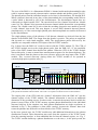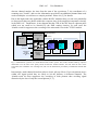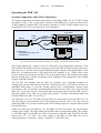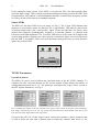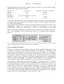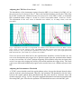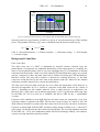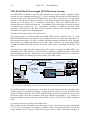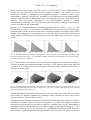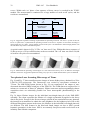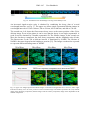
1
High Performance
Photon Counting
User Manual
PML-16-C
16 Channel Detector Head for
Time-Correlated
Single Photon Counting
Becker & Hickl GmbH
PML-16C
Becker & Hickl GmbH
User Handbook
March 2006
High Performance
Photon Counting
1
Tel.
+49 / 30 / 787 56 32
FAX
+49 / 30 / 787 57 34
http://www.becker-hickl.de
email: [email protected]
PML-16-C
16 Channel Detector Head for Time-Correlated
Single Photon Counting
User Handbook
Simultaneous detection in all 16 channels
Works with all bh TCSPC modules
Routing electronics and high voltage power supply included
Gain control and overload shutdown via bh DCC-100 detector controller card
1-by-16 arrangement of detector channels
IRF width 150 ps FWHM
Count rate up to 4 MHz
2
PML-16C
User Handbook
Contents
Introduction............................................................................................................................ 3
Principles of Multidetector TCSPC....................................................................................... 4
Operating the PML-16C ........................................................................................................ 7
System Components and Cable Connections .................................................................... 7
Status LEDs ....................................................................................................................... 8
TCSPC Parameters ............................................................................................................ 8
System Parameters......................................................................................................... 8
Trace and Display Parameters ....................................................................................... 9
DCC-100 Parameters................................................................................................... 12
Internal Discriminator Threshold of the PML-16C ..................................................... 13
Safety ............................................................................................................................... 13
Technical Details of Single-Photon Detection .................................................................... 14
Amplitude Jitter of the Single-Photon Pulses.................................................................. 14
Constant Fraction Triggering........................................................................................... 16
Adjusting the CFD Zero-Cross Level.......................................................................... 17
Adjusting the Discriminator Threshold ....................................................................... 17
Channel Uniformity......................................................................................................... 19
Efficiency................................................................................................................. 19
Transit Time ............................................................................................................ 20
Spectral Response............................................................................................................ 20
Background Count Rate................................................................................................... 21
Dark Count Rate ...................................................................................................... 21
Afterpulsing ............................................................................................................. 22
PML-SPEC Assembly ......................................................................................................... 24
MW-FLIM Multi-Wavelength FLIM Detection Systems.................................................... 26
One-Photon Excitation with Confocal Detection .................................................... 26
Two-photon Excitation with Descanned Detection................................................. 26
Two-photon Excitation with Non-Descanned Detection......................................... 27
Applications......................................................................................................................... 30
Single-point tissue spectroscopy...................................................................................... 30
Chlorophyll Transients .................................................................................................... 30
Two-photon Laser Scanning Microscopy of Tissue ........................................................ 32
Troubleshooting................................................................................................................... 34
Assistance through bh.......................................................................................................... 35
Specification ........................................................................................................................ 36
Electrical .......................................................................................................................... 36
Mechanical....................................................................................................................... 37
References............................................................................................................................ 38
Index .................................................................................................................................... 39
PML-16C
User Handbook
3
Introduction
The PML-16C detector is part of the Becker & Hickl modular multidimensional TCSPC
systems. The PML-16-C detects photons simultaneously in 16 channels of a multi-anode
PMT. The module connects directly to the bh SPC-130, 140, 150, 630, 730, or 830 TCSPC
devices. Signal recording is based on bh’s proprietary multi-dimensional TCSPC technique [2,
3, 10]. For each photon the internal routing electronics generate a timing pulse and a detector
channel signal. These signals are used in the TCSPC device to build up the photon distribution
over the arrival time of the photons and the detector channel number. The result is a set of 16
waveform recordings for the 16 channels of the multi-anode PMT.
The required routing electronics and a high-voltage power supply for the multi-anode PMT is
included in the PML-16-C module. The PML-16-C is controlled via the bh DCC-100 detector
controller [12]. The DCC-100 provides for the power supply, gain control, and overload
shutdown of the PML-16C.
Compared to sequential recording of 16 signals with a single detector the PML-16-C yields a
dramatically increased detection efficiency. Typical applications are optical tomography,
multi-wavelength fluorescence lifetime microscopy, stopped flow experiments, and classic
multi-wavelength fluorescence lifetime experiments. The PML-16 is part of the bh
PML-SPEC spectral detection system and the bh multi-wavelength FLIM systems [3].
This handbook covers the general function of the PML-16C, the interaction with the SPC
module, the setting of the TCSPC system parameters, and the special technical issues of
photon detection with multichannel PMTs. It describes the PML-SPEC spectral detection and
MW-FLIM multi-wavelength FLIM detection systems and demonstrates the application of
these systems to spectroscopy and imaging of biomedical systems. The basics of multidimensional TCSPC are described only briefly. For a comprehensive review of this technique
please refer to [2]. For detailed description of the bh SPC modules, the associated SPCM
software, applications of the bh TCSPC technique please refer to the bh TCSPC Handbook
[3], available on www.becker-hickl.com.
4
PML-16C
User Handbook
Principles of Multidetector TCSPC
Classic time-correlated single photon counting (TCSPC) is based on the detection of single
photons of a periodic light signal, the measurement of the detection times within the signal
period, and the reconstruction of the optical waveform from the individual time measurements
[26]. Advanced TCSPC techniques are multi-dimensional. They measure not only the times of
the photons after the excitation pulses but also the wavelength, the location of emission in a
sample, or the times from the start of the experiment [2, 3]. All TCSPC techniques make use
of the fact that for low-level, high-repetition rate signals the light intensity is usually low
enough that the probability to detect more than one photon per signal period is negligible.
Under this condition only one photon per signal period has considered. The photon is
detected, its parameters, i.e. time, wavelength, location, etc., are measured, and the
distribution of the photon density over these parameters is build up.
Compared with other time-resolved detection techniques TCSPC has a number of advantages,
such as superior time resolution, near-ideal (or ‘shot-noise’ limited) sensitivity and signal-tonoise ratio, superior stability of the instrument response function [2, 3, 7], and multidimensionality. It is often objected against TCSPC that the count rate must be low enough to
make the detection of several photons per signal period unlikely. Often a limit of 0.01 photons
per signal period is given for TCSPC [26], but a detection rate up to 0.1 or even 0.2 per signal
period can usually be tolerated [2, 3]. Thus, with modern excitation sources count rates on the
order of 10⋅106 s-1 can be obtained. Acquisition times at such count rates are in the
millisecond range.
It is difficult to obtain count rates above 1⋅106 s-1 high from biological samples without
causing photobleaching or photodamage [6]. In other words, at typical count rates a single
TCSPC module with a single detector delivers undistorted waveforms.
Now consider an array of PMT channels over which the same photons flux is spread. Because
it is unlikely that the complete array detects several photons per signal period it is also
unlikely that several channels of the array will detect a photon in one signal period. This is the
basic idea behind multi-detector TCSPC. Although several detectors are active simultaneously
they are unlikely to detect a photon in the same signal period. The photon pulses delivered by
the detectors are therefore unlikely to overlap, and the times of the photons detected in all
detectors can be measured in a single TCSPC channel [2, 3, 9].
A block diagram of the PML-16-C is shown in Fig. 1.
Multi-anode PMT
Photocathode Dynodes
Routing Electronics
Anodes
Discriminators
Encoder
to TCSPC
module
D1
..
..
..
..
..
..
D16
High
Voltage
ENC
’Channel’
Detector number
’Disable count’
Photon Pulses
Fig. 1: Block diagram of the PML-16-C
PML-16C
User Handbook
5
The core of the PML-16 is a Hamamatsu R5900 16 channel multi-anode photomultiplier tube
with 16 separate output (anode) elements and a common cathode and dynode system [20, 22].
The photon pulses from the individual anodes are fed into 16 discriminators, D1 through D16.
When a photon is detected in any place of the photocathode the corresponding anode delivers
a pulse which is detected by one of the discriminators. The discriminator output lines are
connected to a digital encoder, ENC. The encoder delivers four ‘channel’ bits and one ‘disable
count’ bit. The ‘channel’ bits represent the detector channel which detected the corresponding
photon. The ‘disable count’ bit is active when the encoding electronics was unable to provide
a valid ‘channel’ data word. This may happen is several PMT channels detected photons
simultaneously, or if the current single-photon pulse had an amplitude too small to be detected
by the discriminators.
The single-photon pulses of the photons of all detector channels are derived from the last
dynode of the R5900 PMT. The output from the dynode is positive. The pulses are amplified
and inverted an a wide band amplifier, AMP. The single-photon pulses delivered by the
amplifier are compatible with the CFD inputs of the bh TCSPC modules.
Fig. 2 shows how the PML-16C works in concert with the TCSPC module [3]. The CFD of
the TCSPC module receives the single-photon pulse from the PML-16C, i.e. the amplified
pulse of the PMT channel that detected the photon. When the CFD of the TCSPC module
detects this pulse, it starts a normal time-measurement sequence for the detected photon. The
time is measured from the photon to the next reference pulse at the stop input of the TCSPC
module. This ‘reversed start-stop’ timing allows the TCSPC module to be operated at
extremely high pulse repetition rates [3].
PML-16C
TCSPC Module
Channel
Channel register
PMT
Channel
latch
Dis.Cnt
Start
CFD
Time
measurement
TAC
Reference
from laser
Stop
ADC
t
CFD
Fig. 2: TCSPC multidetector operation. The TCSPC module builds up the photon distribution over the time in the
pulse period and the PMT channel number. The result is 16 separate waveforms for the 16 PMT channels.
The output pulse of the CFD loads the ‘channel’ information from the PML-16C into the
channel register of the TCSPC module. The channel information is used as an additional
dimension of the recording process. In other words, it controls the memory block in which the
photon is stored. Thus, in the TCSPC memory separate photon distributions for the individual
detectors build up. In the simplest case, these photon distributions are single waveforms, as
indicated in Fig. 2. The technique is often called ‘routing’, because the ‘channel’ data word
routes the photons into different waveform blocks of the TCSPC memory.
In the more general case, the TCSPC module may add additional dimensions to the photon
distribution recorded. These dimensions may come from the sequencer of the TCSPC board,
from the scanning interface, or from additional bits fed into the channel register, see Fig. 3.
The TCSPC module builds up a photon distribution over the time, t, in the pulse period, the
6
PML-16C
User Handbook
detector channel number, the time from the start of the experiment, T, the coordinates of a
scanning area, X and Y, and over the information provided by an additional channel data word
used to multiplex several lasers or sample positions. Please see [3] for details.
Due to the high count rates applicable with the bh SPC modules there is a non-zero probability
to detect more than one photon within the response time of the amplifier/comparator circuitry
in the PML-16C. Furthermore, it may happen that the CFD of the SPC detects a photon pulse
which was too small to be detected by the PML routing circuitry. In such cases the
‘disable count' bit suppresses the recording of the misrouted event in the TCSPC module.
Multiplexing
Multiplexing channel
Channel register
Channel
PML-16C
PMT Channel
latch
Dis.Cnt
Start
CFD
Time
measurement
TAC
Reference
from laser
Experiment
Trigger
Scan Clocks
etc.
Stop
ADC
CFD
Sequencer,
scanning
interface
t
Photon
distribution
PMT
channel 1
Photon
distribution
PMT
channel 2
............
Photon
distribution
PMT
channel 16
T, X, Y, etc.
Fig. 3: Multidetector operation of a multi-dimensional TCSPC system. The TCSPC module builds up a photon
distribution over the time in the pulse period, the detector channel number, the time from the start of the
experiment, the coordinates of a scanning area, and over the information provided by an additional channel data
word.
Interestingly, multi-channel detection reduces classic pile-up effects. If several photons arrive
within one signal period they are likely to hit the detector in different channels. The
‘disable count' bit then suppresses the recording of both photons thus avoiding signal
distortion by the loss of only the second photon [2, 3].
PML-16C
User Handbook
7
Operating the PML-16C
System Components and Cable Connections
The system components and cable connections for operating a PML-16C in a TCSPC system
are shown in Fig. 4. The 15 pin sub-D connector of the PML-16C is connected both to the
TCSPC module [3] and the DCC-100 detector controller [12]. The TCSPC module can be any
of the bh SPC-630, 730, 830, 140/144 or 150/154 modules.
SPC module
PML-16C
Photon
pulses
see (1)
’CFD’
Routing
from
Laser
’SYNC’
C1
Power supply
(1) cable length:
<1.5m for SPC-630, 730, 830, 140
7m for SPC-130
DCC-100
C2
C3
Fig. 4: Cable connections between the PML-16C, the DCC-100 and the TCSPC module.
The routing signals (the ‘channel’ bits) are connected to the routing input connector of the
SPC module. For modules with two connectors (such as the SPC-830) the routing connector is
the lower one, i.e. the one closer to the motherboard of the computer. The photon pulses of the
PML-16C are connected to the ‘CFD’ input of the SPC modules. A 50-Ω SMA cable is used
for this connection. Except for the SPC-130/134 the photon pulse cable should not be longer
than the routing cable in order to maintain correct sampling of the routing bits by the channel
register of the SPC module.
The bh SPC-130 modules and the SPC-134 packages were originally designed for
multiplexing, not for multi-detector operation. Therefore the SPC-130 cards do not have an
adjustable latch delay to read the routing signals from a multichannel detector head.
Nevertheless, SPC-130 modules manufactured later than January 2004 can be used with the
PML-16C. To provide for the correct latch delay the photon pulses from the PML must be
delayed by about 35 ns. This can be achieved by using a 7 m cable in the photon pulse line
from the PML to the SPC-130, see Fig. 4.
The older SPC-330, 430, 530 work with the PML-16C in the same way as the SPC-630, 730
and 830. However, these modules have an ISA connector. Because a DCC-100 card is used to
control the PML-16C operation with the older SPC modules requires a computer that has both
ISA and PCI slots.
Unlike its predecessor, the PML-16 [13], the PML-16C does not require any external highvoltage power supply. The high voltage for the PMT tube is generated internally. The voltage,
i.e. the PMT gain, is controlled via a DCC-100 detector controller card. The DCC-100 also
delivers the +5V, -5V, and +12V power supply to the PML-16. The PML-16C can be
connected both to ‘Connector 1’ and to ‘Connector 3’ of the DCC-100.
8
PML-16C
User Handbook
If the maximum output current of the PMT is exceeded the DCC-100 automatically shuts
down the high voltage. This overload protection mechanism normally prevents the PMT from
being destroyed. Nevertheless, overload shutdown should be considered an emergency and not
be used to switch off the detector in standard situations.
Status LEDs
The PML-16C has three LEDs at its rear panel, see Fig. 5. The ‘Count’ LED indicates that
photons (or at least dark counts) are detected. The ‘Count Disable’ LED indicates the fraction
of photons suppressed by the ‘count disable’ signal. Please note that there are always some
photons that cannot be unambiguously assigned to a particular channel, e.g. photons with
extremely small SER amplitudes. The ‘overload’ LED turns on if the count rate is high so that
an increasing number of photons are either rejected or misrouted. It does not necessarily mean
that the PMT is overloaded. Unless you need maximum routing efficiency you may therefore
ignore the overload LED.
Count
CFD
Cntdis
Ovld
Routing
. .. .. .. .. .
.....
Fig. 5: Rear panel of the PML-16C
TCSPC Parameters
System Parameters
The PML-16C can be used in almost any operation mode of the bh TCSPC modules. To
configure the SPC on-board memory for the correct number of data blocks the number of
routing channels must be set to ‘16’. The parameter is defined in the ‘Page Control’ section of
the SPC System Parameters, see Fig. 6.
Fig. 6: Defining the number of detector channels in the ‘Page Control’ section of the SPC system parameters.
Left: Single, Oscilloscope, f(t,T) f(t, ext), fi(t), fi(ext) and Continuous Flow mode. Middle: Scan Sync In and
Scan Sync Out mode. Right: FIFO (Time-Tag) mode
Except for the SPC-130/134 the ‘Page Control’ section also contains a ‘delay’ parameter that
is used to define the time after a photon pulse at which the ‘channel’ data word (i.e. the
PML-16C
User Handbook
9
routing information) is read into the channel register of the SPC card. The required ‘Delay’
depends on the type of the SPC module:
Module Type
SPC-630
SPC-730
SPC-830
SPC-130/134
SPC-140/144
SPC-150/154
Default Delay
Typical range of Delay for correct operation
0 ns
0 to 10 ns
0 ns
0 to 10 ns
0 ns
0 to 10 ns
no ‘Delay’ Parameter, use 7 m CFD cable
20 ns
0 to 40 ns
20 ns
0 to 40 ns
Please make sure that ‘Delay’ is within the range of correct operation. If the routing signals
are sampled with a wrong delay the ‘count enable’ signal is not valid, resulting in almost total
loss of the detected photons.
As any other PMT, the PML-16C has to be operated with reasonable CFD (constant fraction
discriminator) settings. For all SPC-x30 modules we recommend to start with
CFD limit low = -80 mV and CFD zero cross = -5 mV. The CFD parameters are accessible
either via the ‘System Parameters’ or directly in the main panel of the SPCM software, see
Fig. 7. For optimisation of the CFD parameters please see ‘Constant Fraction Triggering’,
page 16.
Fig. 7: CFD Parameters. The parameters are accessible via the ‘System Parameters’ (left) or directly in the main
window of the SPCM software. (Parameters shown for SPC-x30 modules)
Trace and Display Parameters
With the correct Page Control parameters (Fig. 6) the TCSPC module automatically records
16 separate waveforms for the individual channels of the PML-16C. Depending on the
operation mode used the data can be interpreted differently. In the ‘Single’ or ‘Oscilloscope’
mode the data are considered waveforms (usually fluorescence decay curves) at different
wavelength or different location at the sample. In the sequential modes the data represent
sequences of decay curves at different wavelength or sample position, in the imaging modes
images at different wavelengths. Consequently, the bh SPCM software provides different
ways to display the data. Details are described in [3]; some examples are shown below.
A typical way to display PML-16C data in the ‘Single’ or ‘Oscilloscope mode’ is shown in
Fig. 8. Individual curves are displayed for the individual detector channels. Up to 8 curves can
be displayed simultaneously. The curves are defined in the ‘Trace Parameters’, shown in the
insert of Fig. 8. The detector channel number is defined by ‘Curve’. By clicking into the
‘Colour’ field for each curve a separate colour can be defined. The display of each curve can
be activated and de-activated by clicking on the ‘Active’ button. The SPCM software provides
several ‘Pages’ that may contain different measurements or subsequent steps of a sequential
measurement. The corresponding data sets are selected by ‘Page’.
10
PML-16C
User Handbook
Fig. 8: Display of PML-16C data in the ‘Single’ or ‘Oscilloscope’ mode. Individual curves are displayed for the
individual detector channels. The curves are defined in the ‘Display’ parameters of the SPCM software (see
insert).
The display of PML-16C data in the f(txy) mode is shown in Fig. 9 and Fig. 10. The figures
show autofluorescence data measured at human skin. The fluorescence was detected by a
PML-SPEC assembly, i.e. a polychromator was used in front of the PML-16C (see page 24).
The data is considered a two-dimensional photon distribution over the time in the fluorescence
decay and the wavelength.
The display style is controlled by the ‘Display Parameters’ of the SPCM software, see Fig. 9,
right and Fig. 10, right. The display scale can be linear or logarithmic; the display range can be
set by an autoscale function or by the operator. Different measurement data sets kept in the
memory of the SPC module can be selected by ‘Page’. The Display Parameters provide
different display modes (3D curves, Colour-Intensity, OGL Plot). For Fig. 9 the ‘3D curves’
mode was selected for Fig. 10, the Colour-Intensity mode.
Fig. 9: Display of PML-16C data in the f(txy) mode. The data are shown as a two-dimensional photon
distribution over the time within a fluorescence decay and the channel number of the PML-16C. The display is
controlled by the ‘Display parameters (right). ‘Curve’ mode and linear intensity scale selected. Autofluorescence
of skin recorded by PML-SPEC assembly, the channel number represents the wavelength.
PML-16C
User Handbook
11
Fig. 10: Display of PML-16C data in the f(txy) mode. The data are shown as a three-dimensional photon
distribution over the time within a fluorescence decay and the channel number of the PML-16C. The display is
controlled by the ‘Display parameters (right). ‘Colour-Intensity’ mode and linear intensity scale selected.
Autofluorescence of skin recorded by PML-SPEC assembly. The channel number represents the wavelength.
Please note that the data structures in the ‘Single’, ‘Oscilloscope’, and ‘f(t,x,y)’ modes are
identical. Therefore you may run a measurement in the ‘Single’ mode and display the data in
the ‘f(t, x, y)’ mode or vice versa.
An example of a ‘Scan Sync In’ mode measurement is shown in Fig. 11. The images were
taken in a Zeiss LSM 510 NLO two-photon laser scanning microscope upgraded with a bh
SPC-830 TCSPC module and a bh MW-FLIM assembly. The sample was an unstained mouse
kidney section. Eight display windows were defined showing the integral fluorescence of the
sample in eight wavelength intervals. Each image has its own display parameters. The
parameters of the left image of the second row are shown right.
Fig. 11: Multi-wavelength measurement in the ‘Scan Sync In’ mode. LSM 510 two-photon laser scanning
microscope, SPC-830 TCSPC module, bh MW-FLIM assembly. The sample is a mouse kidney section. Images
in different wavelength intervals are shown left. Each image has its own display parameters; the parameters of the
left image of the second row are shown right.
The display mode is the ‘Colour Intensity’ mode. The colours are defined in the lower left of
the display parameter panel. They were selected according to the true colour of the wavelength
intervals. The wavelength intervals themselves are defined in the ‘Window Parameters’ of the
SPCM software (not shown here). The defined wavelength intervals are assigned to the
current image by ‘Routing X Window’, in the lower right of the display parameter panel.
Images can also be displayed in time-windows specified in the ‘Window Parameters’. The
window for the current image is selected under ‘T Window’, in the lower right of the panel.
12
PML-16C
User Handbook
For details of the display functions please see [3]; for fluorescence lifetime analysis of the
images please see [15].
DCC-100 Parameters
The DCC-100 has its own control software [12]. The DCC-100 software is included in the
TCSPC installation package, see [3], bh TCSPC Handbook, ‘Software Installation’. It can be
added to an existing TCSPC installation at any time. The DCC-100 software panel is shown in
Fig. 12. The DCC-100 panel can be placed anywhere in the screen area. To keep the panel
visible at any time we recommend to switch on the ‘always on top’ function in the
‘Parameters’ of the DCC-100.
Fig. 12: DCC-100 control panel. Left: After starting the DCC software. Middle: After enabling the outputs.
Right: After an overload shutdown.
After starting the DCC-100 software the panel comes up with ‘Outputs disabled’, see Fig. 12,
left. This is a safety feature to avoid unintentionally switching on a detector or a high voltage
power supply unit that may be connected to the DCC. (The DCC-100 can be configured to
start with the outputs enabled, but this configuration should not be used for controlling PMTs
or any other detectors that use external or internal high voltage.)
The DCC-100 is able to control two detectors, several shutters or actuators, and the
thermoelectric coolers of one or two detector modules. The DCC-100 modules has three
connectors: Connector 1 and connector 3 are for the detectors, connector 2 is for the shutters.
The PML-16C can be operated both at connector 1 and at connector 3. For both connectors the
control panel contains a ‘Gain’ slider and three buttons for activating the supply voltages. The
settings shown in Fig. 12 are for operation of the PML-16C at connector 1.
To operate the PML-16C the supply voltages, +12 V, +5 V, and -5 V, at the used connector
must be activated (click on the corresponding buttons). There is no special switch-on
sequence. You can turn the supply voltages on and of at any time.
Before enabling the outputs we recommend to turn down the detector gain by pulling down
the ‘Gain’ slider. This precaution avoids running into a possible overload condition at full
detector gain. After turning down the gain, enable the outputs by clicking on the ‘Enable
Outputs’ button and pull up the ‘Gain’ slider. When the gain approaches 80 to 85% you may
see the first photons being detected in the SPC module. Check the CFD count rate of the SPC
module while further increasing the gain. If the count rate exceeds 5⋅106 s-1 decrease the light
intensity at the detector. Full operation of the PML-16C is obtained at a gain of 90% to 100%.
PML-16C
User Handbook
13
The ‘Gain’ slider controls the operating voltage of the PMT. The actual gain of a PMT
increases with approximately the 4th power of the operating voltage.
Please note:
Photon counting records the pulses the detector delivers for the individual photons of the light
signal. The detector gain determines the amplitude of these pulses, not their frequency. The
detector gain can therefore not be used to control the magnitude of the recorded photon
distributions. Any attempt to decrease the sensitivity by reducing the detector gain results in
decreased signal-to-noise ratio and poor channel uniformity (see ‘Technical Details of SinglePhoton Detection’, page 14).
If the light intensity at the PML-16C is too high the DCC-100 shuts down the gain and the
+12 V supply voltage. In extreme cases this may happen at a gain far below the single-photon
detection level, i.e. before the SPC module displays a CFD count rate. The DCC-100 panel
after an overload shutdown is shown in Fig. 12, right. If an overload shutdown has occurred,
remove the source of the overload. Then click on the ‘Reset’ button. After the reset the
PML-16 resumes normal operation. Please do not attempt to avoid overload by operating the
PML-16C at reduced detector gain. This would result in poor counting efficiency and poor
channel uniformity, see Fig. 21.
Internal Discriminator Threshold of the PML-16C
The PML-16C has 16 internal discriminators to generate the routing information (see Fig. 1,
page 4). The threshold of these discriminators can be adjusted by a trimpot. The internal
threshold is factory adjusted. Changing the threshold is not normally needed and therefore
discouraged. If the threshold has been changed for any reasons it can be re-adjusted as
described below.
Run a measurement in the oscilloscope mode of the SPC module. Use the stop option ‘Stop T’
and a collection time of about 1 second. Activate the ‘Trace Statistics’ panel. Activate the
PML-16C but do not send light into the PML-16C. Turn the threshold potentiometer left until
the ‘Overload’ LED at the back of the PML-16C turns on. The threshold is then close to zero.
Then turn the potentiometer back (toward higher threshold) until the overload LED turns off.
Send defined light signals to the PML-16C. Adjust the internal threshold in order to obtain a
maximum of the ‘total counts’, good channel separation and good channel uniformity. The
final settings may be slightly above, but not far from the point where the overload LED turns
off.
Safety
The R5900 PMT of PML-16C is operated at a cathode voltage of up to 1000 V. The cathode
voltage is generated by a DC-DC converter inside the PML-16C. Therefore do not open the
housing of the PML-16C when the 15 pin cables from the DCC-100 and the SPC module are
connected. Moreover, please operate the PML-16 only with the correct routing and power
supply cables. Make sure that the cables are connected to the correct connectors of the
DCC-100 and the SPC module. Using wrong cables or connecting the cables to a wrong
connector (e.g. a monitor output from a display card) can seriously damage the PML-16C, the
DCC-100, the SPC module or the display card. Make sure not to connect a computer monitor
to one of the 15 pin connectors of the DCC-100 of the SPC card. Please do not disconnect any
cables when the PML-16C is in operation.
14
PML-16C
User Handbook
Technical Details of Single-Photon Detection
In early times of TCSPC users were confused by countless and often contradicting instructions
about optimising the PMTs of their instruments, configuring constant fraction discriminators,
tweaking discriminator thresholds, trigger fractions, and preamplifier bandwidth or gain. The
difficulties in part resulted from the slow speed of the early TCSPC electronics and the
relatively slow rise times of the single-electron response of the PMTs used. Other advice, such
as reducing the relative dark count rate by increasing the CFD threshold, resulted from poorly
performing PMTs and preamplifiers or was plainly wrong. Confusion resulted also from
applying timing solutions optimised for high-energy particle detection by scintillators
straightforward to single-photon detection.
With the currently available high speed constant-fraction discriminators, low-noise
preamplifiers, and fast PMTs, adjustments, if required at all, are largely simplified. In fact, all
a TCSPC user has to do is to set a discriminator threshold above the noise level of the
preamplifier and to increase the operating voltage of the PMT until the counting efficiency
starts to saturate.
Nevertheless, the technical details of operating a multichannel PMT in a TCSPC system are
described in the following paragraphs. The examples given in this sections are recorded with
typical devices. The PMT gain and CFD parameters given are considered representative.
Please note, however, that individual PMTs may slightly differ in gain, efficiency, and spectral
response.
Amplitude Jitter of the Single-Photon Pulses
A conventional photomultiplier tube (PMT) is a vacuum device which contains a
photocathode, a number of dynodes (amplifying stages) and an anode which delivers the
output signal [2, 3, 22]. The principle is shown in Fig. 13.
D2
PhotoCathode
D1
D3
D4
D6
D5
D7
D8
Anode
Fig. 13: Principle of a conventional PMT
The operating voltage builds up an electrical field that accelerates the electrons from the
photocathode to the first dynode D1, further to the next dynodes, and from D8 to the anode.
When a photoelectron hits D1 it releases several secondary electrons. The same happens for
the electrons emitted by D1 when they hit D2. The overall gain reaches values of 106 to 108.
The secondary emission at the dynodes is very fast; therefore the secondary electrons resulting
from one photoelectron arrive at the anode within a few ns. Due to the high gain and the short
response a single photoelectron yields an easily detectable current pulse at the anode.
The detector output pulse for a single photon, (or a single photoelectron) is called the ‘Single
Electron Response’ or ‘SER’. Due to the random nature of the secondary emission, the pulse
amplitude varies from pulse to pulse. The secondary emission coefficient at the dynodes is of
the order of 5 to 10, resulting in a variation of the number of secondary electrons on the order
of 1:2 to 1:4. Moreover, some of the primary electrons are scattered without any
multiplication, which further increases the effective width of the amplitude distribution.
PML-16C
User Handbook
15
The single-photon (SER) pulses of a PML-16C detector are shown in Fig. 14. The pulses have
a rise time of about 600 ps and a width of about 2 ns.
Fig. 14: Single-photon pulses delivered by the PML-16C. Gain = 95%, recorded with Tektronix ??? oscilloscope.
Horizontal 2 ns / div, vertical 20 mV / div.
The amplitude of the pulses varies over a wide range. The pulse amplitude distribution
measured at three different channels of the same PML-16C is shown in Fig. 15.
Fig. 15: Amplitude distribution of the single-photon pulses of a PML-16C. Channel 1 (blue), channel 4 (green)
and channel 16 (red). DCC gain setting 95%, corresponding to a cathode voltage of -950 V.
Fig. 15 shows that the width at half maximum of the amplitude distribution is 1:3 to 1:4. The
pulse amplitude distribution consists of three major components. The largest part of the
distribution, above about 1 unit, is due to the regular single-photon pulses. It also contains
background pulses due to thermal emission at the photocathode. The amplitude distribution is
slightly different for different channels, which has to be taken into regard when the CFD
threshold is optimised (see Fig. 21).
Especially at high gain there is usually a sub-structure in the amplitude distribution. It is
probably caused by spatial nonuniformity in the secondary emission coefficient, and by the
discrete number of secondary electrons emitted at the first dynode.
Thermal emission, photoelectron emission, and reflection of primary electrons at the dynodes
cause an increase of the pulse density at low amplitudes. At very low amplitudes electronic
16
PML-16C
User Handbook
noise, either from the preamplifier or from the environment, causes a third peak of extremely
high count rate.
The amplitude jitter of the SER pulses sets two general requirements to the input
discriminator circuitry in the TCSPC module. On the one hand, the trigger delay must be
independent of the variable amplitude of the pulses. On the other hand, the discriminator
threshold must be high enough to reject the electronic noise and the pulses caused by thermal
emission in later stages of the dynode chain of the PMT.
Constant Fraction Triggering
In a simple leading-edge trigger the amplitude jitter of the single-photon pulses would
introduce a timing jitter on the order of the rise time of the pulses. Therefore ‘Constant
Fraction Discriminators’, or ‘CFDs’ are used in the start and stop inputs of the bh TCSPC
modules. A CFD virtually triggers at a constant fraction of the peak amplitude of the input
pulse. In practice constant fraction triggering is achieved by triggering on the zero cross of the
difference of the delayed and the undelayed input pulse [2, 3]. The principle is shown in Fig.
16.
Input difference
voltage of D1:
DEL1 DEL2
Threshold
Input pulse
Zero Cross
+
- D1
Input
Delayed
pulse
Enable
Zero cross
Threshold
+
- D2
Difference
Zero
cross level
Fig. 16: Principle of the CFDs of the bh TCSPC boards
The CFD contains two fast differential discriminators, D1 and D2. D2 triggers when the input
amplitude exceeds a selectable ‘CFD threshold’. After a small delay, DEL1, the same input
pulse is fed into the differential inputs of D2. However, the signal at the non-inverting input of
D1 is given an additional delay, DEL2. D1 triggers when the difference of the voltages at its
inputs crosses the baseline, as shown in Fig. 16, right. A fast D-flip-flop is enabled by the
pulse of D2 and triggered by the transition of D1. Thus, the flip-flop is triggered when a zero
cross at D1 occurs while the input voltage exceeds the CFD threshold.
Ideally, the temporal location of the zero cross does not depend on the amplitude. The circuit
shown in Fig. 16 therefore meets the requirements of single-photon timing: Pulses below a
defined amplitude are rejected, and the amplitude jitter has no influence on the timing.
Theoretically minimum timing jitter should be expected at a zero-cross level of exactly zero.
However, in practice the zero-cross discriminator has an offset voltage of a few mV.
Moreover, the intrinsic delay of the discriminator depends on the amplitude of the input
signal. The corresponding contribution of the discriminator to the timing jitter can be
compensated for by a ‘CFD Zero-Cross Level’ slightly offset from the signal baseline.
PML-16C
User Handbook
17
Adjusting the CFD Zero-Cross Level
The dependence of the instrument response function (IRF) of one channel of a PML-16C on
the zero-cross level is shown in Fig. 17. Due to the fast discriminators used in the CFDs of the
bh TCSPC modules the influence of the zero-cross level on the IRF is small. A reasonable
IRF is obtained within a range of +30 mV to -30 mV, best results within +10 mV to -10 mV.
The adjustment of the zero cross is therefore not critical, or, in many cases, even not
necessary.
Fig. 17: Dependence of the IRF of a single PML-16C channel on the CFD Zero-Cross Level. Black +30 mV,
green +10 mV, red -10 mV, magenta -30 mV. The FWHM of the IRF is shown in the inserts. Left: Linear scale,
200 ps / division, 1.22 ps / point. Right: Logarithmic scale, 500 ps / division, 1.22 ps / point. Light pulses from
BHL-600 diode laser, pulse width 30 ps, repetition rate 50 MHz.
Zero-cross levels closer than 5mV to the signal baseline should be avoided. In that case, the
zero-cross discriminator may trigger due to spurious signals from the synchronisation channel
or may even oscillate. Of course, spurious triggering and oscillation stop when an input pulse
arrives, but some after-ringing may still be present and modulate the trigger delay. The result
can be poor differential nonlinearity (ripple in the recorded curves) or a double structure in the
IRF.
Adjusting the Discriminator Threshold
A TCSPC system should record the regular photon pulses, but not the thermal dynode pulses
and the electronic noise background. Therefore, the optimum CFD threshold is near the valley
between the regular photon pulse distribution and the peak caused by electronic noise and
dynode emission, see Fig. 18, left. The pulse amplitude distribution stretches horizontally with
increasing PMT gain. Therefore the optimum CFD threshold increases with the PMT gain.
18
PML-16C
second
Rate vs. PMT gain
Rate vs. threshold
Amplitude distribution
Pulses
per
User Handbook
Count
electronic noise
Rate
pulses from dynodes
Count
electronic noise
Optimum Gain
Rate
pulses from dynodes
1
regular photon
pulses
Gain 2
12
Optimum
threshold
Gain1
2
regular photon pulses
Threshold 1
1 2
Optimum Thres.
Gain 2
Threshold 2
Gain1
Pulse amplitude
CFD Threshold
PMT Gain
Fig. 18: Left: General shape of the amplitude distribution of the single-photon pulses. Middle: Dependence of the
count rate on the CFD threshold. Right: Dependence of the count rate on the PMT gain.
The corresponding dependence of the count rate on the discriminator threshold is shown in
Fig. 18, middle. The PMT is illuminated with light of low intensity. When the discriminator
threshold (‘CFD limit Low’) is decreased the count rate increases. At a sufficiently low
threshold the increase of the count rate flattens, and in the ideal case forms a plateau. The
PML-16C-0 and -1 detectors the counting plateau is clearly visible. For other PMTs the
plateau may be not very pronounced. However, at least a flattening of the count rate increase
should be found.
At very low threshold the count rate increases again because thermal dynode pulses or
electronic noise are detected. In practice the dynode peak may be not very prominent or even
be hidden in the electronic noise.
A similar behaviour is found if the gain of the PMT is changed, see Fig. 18, right. The count
rate increases with increasing gain and eventually reaches a plateau.
Consequently, there are two ways to find a reasonable operating point of the PMT: You may
either set a reasonable PMT gain and vary the CFD threshold, or set a reasonable CFD
threshold and vary the PMT gain. For the PML-16C the DCC gain should be between 90 and
95 %, corresponding to a PMT operating voltage between 900 and 950 V. The CFD threshold
should be within a range of -50 to -100 mV.
The CFD threshold, does, of course also influence the shape of the IRF. An example is given
in Fig. 19. The CFD threshold was increased in 20 mV steps from -20 mV to -140 mV. At
very low threshold (-20 mV and -40 mV) the IRF develops a shoulder prior to the mean peak.
The shoulder is typical of front-window PMTs operated at low threshold. Most likely, it is
caused by photoelectron emission at the first dynode. A clean IRF at good efficiency is
obtained for thresholds from -60 mV to -100 mV. The efficiency drops noticeably at -120 mV
and -140 mV. Despite of the short IRF width (see inserts in Fig. 19) operating the PML-16C
in this threshold range is discouraged. The high threshold not only results in loss of photons
but also in large efficiency differences between the channels (see paragraph below).
PML-16C
User Handbook
19
Fig. 19: IRF for CFD thresholds from -20 mV to -140 mV. The FWHM of the IRF is shown in the insert. Left:
Linear scale, 200 ps / division, 1.22 ps / point. Right: Logarithmic scale, 500 ps / division, 1.22 ps / point. Light
pulses from BHL-600 diode laser, pulse width 30 ps, repetition rate 50 MHz.
Channel Uniformity
Efficiency
For a multichannel PMT the CFD threshold has also a noticeable influence on the uniformity
of the channels in terms of efficiency. Although all PMT channels use the same dynode
system and the same operating voltage the pulse amplitude distribution for the individual
channels may differ noticeably (see Fig. 15). The situation is illustrated in Fig. 20. PMT
channel B has a gain 25% lower than channel A. Threshold 2 yields a satisfactory efficiency
for channel A, but not for channel B. If this threshold is used the result is an large variation in
the efficiency of the channels. Better results are obtained with threshold 1. Both channels are
then in the ‘counting plateau’, and the gain difference has little influence on the efficiency.
For the PML-16C it is therefore important to set the PMT gain high enough for the CFD
threshold used (or the CFD threshold low enough for the gain used) to obtain reasonable
counting efficiency for the channel of the lowest gain.
Count
Rate
Threshold 1
Threshold 2
Channel A
Channel B
CFD Threshold
Fig. 20: Effect of gain variations of the PMT channels
A practical example is given in Fig. 21. The channels of a PML-16C were evenly illuminated
with continuous light. The DCC gain was set to 95%, corresponding to a PMT operating
voltage of 950 V. From left to right, the CFD threshold was increased from -40 mV to
-120 mV. It can clearly be seen that with increasing CFD threshold there is not only a decrease
in efficiency but also a degradation in the channel uniformity.
20
PML-16C
User Handbook
Fig. 21: Uniformity of the efficiency of the PML-16C channels. DCC gain setting 95%. Left to right: CFD
threshold -40 mV, -60 mV, -80 mV, -100 mV, -120 mV
Transit Time
Photomultipliers of the metal channel type have a noticeable dependence of the transit time on
the location on the photocathode [3]. The R5900 tube used in the PML-16C is no exception.
Fig. 22 shows that there is a systematic wobble in the transit time of the channels. The effect
has to be taken into account in the data analysis, either by determining individual IRFs for the
channels or by including a shift parameter in the fit procedure.
Fig. 22: Instrument response functions of the PML-16 C channels. Response to 50 ps diode laser pulses at
650 nm. Left: curve plot. Right colour-intensity plot, vertical axis is the channel number.
Because of the transit time differences we do not recommend to combine PMT channels
directly, i.e. by changing the connections of the routing bits. The result would be a loss in time
resolution.
Spectral Response
The PML-16C comes in two photocathode versions. The typical spectral response is shown in
Fig. 23. The bialkali cathode of the PML-16C-0 has a high efficiency in the blue range of the
spectrum and can be used from about 320 nm to 600 nm. The multi-alkali cathode (PML-16C1) has its efficiency maximum in the green region of the spectrum. It can be used from bout
320 nm to 800 nm. Please note that the formation of the photocathode of a PMT is a
complicated and in some details empirical process. Even with modern manufacturing
techniques results are not accurately predictable. Thus, the spectral sensitivity of individual
PMTs may differ slightly in the peak value and in the spectral shape.
PML-16C
User Handbook
Sensitivity
100
mA/W
21
QE=0.1
QE=0.2
bialkali
multialkali
10
1
300
400
500
600
700
Wavelength
800
900
nm
Fig. 23: Typical spectral sensitivity of the bialkali and the multialkali photocathode, after [22].
Spectral sensitivity specifications of PMTs are given in mA photocurrent per Watt incident
power. The quantum efficiency, QE, can be calculated from the spectral sensitivity by
QE = S
hc
S
Wm
=
⋅ 1.24 ⋅ 10 − 6
eλ
λ
A
with S = Spectral Sensitivity, h = Planck constant, e = elementary charge, λ = Wavelength,
c = velocity of light.
Background Count Rate
Dark Count Rate
The dark count rate of a PMT is dominated by thermal electron emission from the
photocathode. Consequently, the amplitude distribution of the output pulses is essentially the
same as for the photoelectrons. Only at very low amplitudes there is a contribution of thermal
emission from the dynodes. With a correctly adjusted CFD threshold these pulses are rejected
anyway. Attempts to reduce the dark count rate by further increasing the CFD threshold are
therefore useless. The only effect would be a decrease in counting efficiency, i.e. the dark
count rate would decrease by the same ratio as the photon count rate. Moreover, the channel
uniformity would be impaired, for reasons described above.
The only way to keep the dark count rate low is to reduce the temperature of the detector. A
decrease in temperature by 10 °C results in a decrease in the dark count rate by a factor of
about 5, depending on the cathode material. Even a small decrease in temperature can
therefore have a large effect. At an ambient temperature of 22°C typical total dark count rates
for the PML-16C are 20 to 200 for -0 (bialkali) and 400 to 2000 for the -1 (multialkali)
versions.
Exposure of the cathode to room light increases the dark count rate temporarily, even if no
operating voltage is applied to the PMT. The increase can be as large as a factor of 100. The
dark count rate resumes its normal value after some time. Full recovery can take several hours.
Exposure to strong light with the PMT operating voltage being switched on (i.e. with a DCC
gain setting >0) can increase the dark count rate permanently. The overload shutdown function
of the PML-16C - DCC-100 combination makes this kind of damage unlikely. Nevertheless,
extreme overload should be carefully avoided.
22
PML-16C
User Handbook
Afterpulsing
The dark count rate is often considered the only source of signal background. Signal
background can, however, also be caused by afterpulsing. All photon-counting detectors (also
single-photon avalanche photodiodes) have an increased probability of producing background
pulses within a few microseconds following the detection of a photon. These afterpulses are
detectable in almost any conventional PMT. It is believed that they are caused by ion
feedback, or, by a smaller amount, by luminescence of the dynode material and the glass of
the tube.
Afterpulsing becomes noticeable especially in high-repetition rate TCSPC applications, in
particular with Ti:Sapphire lasers or diode lasers. At high repetition rate, the afterpulses from
many signal periods pile up and can cause a considerable signal-dependent background. The
total afterpulsing rate can easily exceed the dark count rate of the detector by a factor of 100
[2, 3].
The R5900-L16 tubes used in the PML-16C have a relatively low afterpulsing probability and
thus deliver an excellent dynamic range in high-repetition rate applications. Fig. 24, upper
row, shows a recording of a fluorescence signal, taken with a PML-16C-0 in PML-SPEC
multi-spectral detection assembly (see paragraph below).
Fig. 24: Background by afterpulsing. Left: Fluorescence signal. Right: Dark counts. Upper row: All 16
wavelength channels. Lower row: Channel with maximum fluorescence intensity. Laser pulse repetition rate
20 MHz, acquisition time 100 seconds.
The acquisition time was 100 seconds. The excitation pulse rate was 20 MHz, the acquisition
time 100 seconds. The complete multi-spectral decay data are shown left, the channel of
PML-16C
User Handbook
23
highest intensity right. The useful dynamic range (peak to background) is more than 4 orders
of magnitude, about as good as for an MCP PMT [3].
A dark recording taken with the same acquisition time and pulse repetition rate as the
fluorescence recording is shown in the lower row of Fig. 24. It is obvious that the dark count
level is lower than the background of the fluorescence recording. The average background
levels are 1.8 and 0.015, respectively. Thus, also for the PML-16C the dynamic range at high
pulse repetition rate is limited by afterpulsing, not by the dark count rate.
The straightforward way to reduce the afterpulsing background is to reduce the signal
repetition rate. However, to keep pile-up effects low the count rate must be reduced [2, 3]. The
tradeoff is therefore an increased acquisition time.
24
PML-16C
User Handbook
PML-SPEC Assembly
The PML-SPEC multi-wavelength detection assembly is a combination of the PML-16C and a
small grating polychromator (or spectrograph). The assembly is shown in Fig. 25.
Fig. 25: PML-SPEC multi-wavelength detection assembly, shown with a fibre bundle at the input
The PML-SPEC is available with three different gratings, see table below. The grating
determines the dispersion and thus the wavelength interval recorded via the 16 channels of the
PML-16C. The start wavelength of the interval is selectable by a micrometer screw at the
polychromator.
Grating
Part No.
77417
77414 (standard)
77411
Primary wavelength region
adjustable by set screw
340-820 nm
340-820 nm
340-820 nm
Width of recorded wavelength
interval, channel 1 to 16
300 nm
200 nm
100 nm
Blaze Wavelength
500 nm
400 nm
350 nm
The blaze wavelength is the wavelength the grating is optimised for. The amount of light
diffracted into the first diffraction order is at maximum at this wavelength. However, even at a
wavelength close to the blaze wavelength a grating disperses some light into higher diffraction
orders. The light of the unused orders can cause substantial straylight problems. In
fluorescence applications the PML-SPEC should therefore be used with an additional filter
that blocks the excitation wavelength.
There are several ways to deliver the light into the input slit plane of the polychromator. Freebeam coupling is often used in the traditional fluorescence lifetime setups. In these cases a
lens transfers the luminescent spot in the sample into the input slit of the polychromator. The
parameters of this lens have a considerable influence on the optical efficiency.
The polychromator accepts light within a focal ratio (or ‘f number’) of about 1:3.5. To obtain
maximum light throughput, the f number of the input light cone must match the f number of
the monochromator. Moreover, the image in the input plane must not be larger than the slit.
Building an appropriate relay lens system is no problem if the light comes from a point source.
For larger sources the throughput is limited by the slit size and the f number of the
monochromator; see Fig. 26.
PML-16C
User Handbook
Lens
Source
of
Emission
25
Polychromator, f / n
f/n
a) f number matched
slit fully illuminated
Image on
monochromator
slit
Lens
>f/n
unused
Source
of
Source
of
f/n
used
Polychromator, f / n
f/n
Emission
Emission
b) slit fully illuminated, but
f number too high
Lens
Polychromator, f / n
Image on
input
slit
c) f number matched, but
slit over-illuminated
Image on
input
slit
Fig. 26: Limitations of the light throughput of a polychromator. Once the slit is fully illuminated and the
f numbers are equal, neither (a) a larger lens nor (b) a lens with a higher NA at the source side will increase the
throughput.
Once the input light cone matches the f number of the polychromator (a), neither (b) a larger
lens nor (c) a lens with a higher NA at the source side will increase the amount of transmitted
light. Case (b) leads to an input cone of a larger f number than accepted by the polychromator.
Case (c) results in an image larger than the polychromator slit. In both cases the additional
light transferred by the lens is not transmitted through the polychromator.
Please note that relatively wide input slits can be used for the PML-SPEC. The centre distance
of the PML-16C channels is 1 mm. Reducing the slit width far below this value does not yield
any gain in resolution. Thus, the optimum slit width is in the range of 05. to 1 mm.
Another way to increase the throughput is to reduce the size of the excited spot in the sample
or to match the shape of the source spot to the monochromator slit. In cuvette fluorescence
systems with a horizontal excitation beam a large improvement can be made by turning the
polychromator 90°, so that the slit is horizontal and matches the orientation of the excited
sample volume.
Another way to couple light into the PML-SPEC is via an optical fibre. For fibre-coupled
systems the input slit of the polychromator is replaced with a fibre adapter, with the end of the
fibre placed in the slit plane. The coupling efficiency from the fibre into the polychromator is
then almost ideal. However, coupling the light into the fibre has to cope with the same basic
optical problems as coupling the light directly into the polychromator slit. Fibre diameters up
to 1 mm can be used without much compromise in wavelength resolution. Fibre-coupled
systems are used to connect the PML-SPEC to confocal scan heads of laser scanning
microscopes [8], see Fig. 27. Fibre-coupling has also been used for diffuse optical tomography
(DOT). A super-continuum was generated by sending the pulses of a Ti:Sapphire laser though
a photonic crystal fibre. After propagating of the continuum pulses through the tissue the light
was collected via a multi-mode fibre, and the time-of-flight distributions were recorded in 16
wavelength intervals [1].
An elegant way to increase the throughput of a fibre-coupled system is to use several fibres or
a fibre bundle (see Fig. 28 and Fig. 30). The fibres are arranged along the slit of the
polychromator. The fibre system is thus used to collect light from an increased area and
transform the cross-section of this area into the cross section of the slit.
26
PML-16C
User Handbook
MW-FLIM Multi-Wavelength FLIM Detection Systems
The PML-SPEC assembly is used for bh’s modular fluorescence lifetime imaging (FLIM)
systems for laser scanning microscopy [3, 5]. Laser scanning microscopes scan the sample by
a focused laser beam and detect the fluorescence from the excited spot by a single-point
detector. Confocal microscopes use a pinhole in the detection light path to suppress light from
outside the focal plane [27]. Two-photon microscopes excite the fluorescence by a
femtosecond laser of high repetition rate. Two photons of the input light are used to generate
one fluorescence photon [18, 19]. Two-photon excitation is nonlinear and thus yields
noticiable excitation only in the focus of the microscope objective lens. Therefore excitation
outside the focal plane is avoided altogether.
One-Photon Excitation with Confocal Detection
The general setup of a confocal multi-wavelength FLIM system is shown in Fig. 27. A bh
BDL-405-SM diode laser [14] delivers picosecond pulses into one of the laser input fibres of
the scanning microscope. In order to obtain diffraction-limited focusing the laser scanning
microscopes use single-mode fibres for the laser input. Therefore the -SM (single-mode)
version of the BDL-405 must be used. The power of the laser is controlled via the DCC-100
card.
The fluorescence light from the scanned spot of the sample is fed into the PML-SPEC via a
multi-mode fibre output from the scan head. Fibre outputs are available for almost all modern
laser scanning microscopes. Diode-laser based confocal MW-FLIM systems are available for
the Zeiss LSM 510, the Olympus FV1000, and the Leica SP2 or SP5.
BDL-405-SM picosecond diode laser
Power control
Input fibre
Scan
head
DCC-100
single mode
Output fibre
multi mode
Polychromator
PML-16C
TCSPC Module
Grating
Microscope
Fig. 27: Multi-wavelength FLIM system, one-photon excitation by picosecond diode laser, confocal detection
The TCSPC module is operated in the ‘Scan Sync In’ mode. In this mode the recording in the
TCSPC module is synchronised with the scanning by pixel clock, line clock, and frame clock
pulses from the microscope. The TCSPC module builds up a photon distribution over the time
in the laser pulse period, the coordinates of the scan, and the wavelength [2, 3, 5]. Because of
the large amount of data to be kept in the TCSPC memory an SPC-830 module should be
used.
Two-photon Excitation with Descanned Detection
With a femtosecond Ti:Sapphire laser the sample can be excited by two-photon absorption
[18, 19]. In a microscope, two-photon excitation works with high efficiency because the
energy density in the focus of a high-NA objective lens is high. Noticeable excitation is
PML-16C
User Handbook
27
obtained only in the focus. Therefore two-photon excitation inherently delivers depth
resolution. Confocal detection through a pinhole is not required. Nevertheless, the
fluorescence light can be fed back through the scanner and the pinhole. The optical setup of
the detection light path is then identical with the one used for one-photon excitation. System
with two-photon excitation and detection via the confocal beam path have been used for
FRET experiments [8, 17] and for PDT experiments on the cell level [28].
Two-photon Excitation with Non-Descanned Detection
Because two-photon excitation does not generate fluorescence outside the focus no light from
outside the focal plane needs to be rejected. The fluorescence light can therefore be diverted
directly behind the microscope objective by a dichroic mirror. This setup is called ‘nondescanned’ or ‘direct’ detection in contrast to the ‘confocal’ or ‘descanned detection’ used for
one-photon excitation.
Two-photon excitation in conjunction with non-descanned detection can be used to image
tissue layers several 100 µm deep [18, 21]. Since the scattering and the absorption coefficients
at the wavelength of the two-photon excitation are small the laser beam penetrates through
relatively thick tissue. Even if there is some loss on the way through the tissue it can be
compensated by increasing the laser power. Of course, the fluorescence photons are scattered
on their way out of the tissue and therefore emerge from a relatively large area of the sample
surface. Moreover, the surface is not in the focus of the objective lens. The fluorescence light
therefore leaves the full back aperture of the microscope lens in a cone of relatively large
angle. A multi-wavelength system for non-descanned detection systems has to transfer this
light into the polychromator.
The first multi-spectral FLIM system for two-photon microscopes with non-descanned
detection was described in [16]. An image of the aperture of the microscope objective lens
was projected on the input of a 1-mm multi-mode fibre. The fibre delivered the fluorescence
light to a polychromator. The spectrum was recorded by a bh PML-16 detector, and the 16
wavelength channels were recorded simultaneously by a bh SPC-830 module. The problem of
the optical setup used was that a strong demagnification into the fibre has to be used. This
results in a high numerical aperture of the light cone at the input of the fibre. However, a
multi-mode fibre used near its maximum NA develops strong pulse dispersion [24]. The IRF
of the system is therefore noticeably broader than the IRF of the PML-16. Moreover, the short
focal length required for the projection into the fibre results in a small diameter of the lens.
The system therefore loses efficiency for deep layers of highly scattering samples.
The bh NDD MW-FLIM systems use a fibre bundle to transform the circular cross section of
the microscope lens aperture into the linear cross section of the polychromator slit. The
principle is shown in Fig. 28.
28
PML-16C
User Handbook
DCC-100
750 nm to 900 nm
Scan
head
Ti:Sa Laser
Filter
Fibre bundle
Polychromator
PML-16C
Lens
Shutter
Microscope
Cross
section
of bundle
TCSPC Module
Grating
Fig. 28: Multi-wavelength FLIM system, two-photon excitation and non-descanned detection
A field lens projects an image of the effective aperture of the microscope lens on the input of a
fibre bundle. The fibre bundle has a circular cross section at the input, and a rectangular cross
section at the output. Thus, the input matches the image of the microscope lens aperture. The
output matches the input slit of the monochromator. The system features high efficiency even
for highly scattering samples. Moreover, the fibre bundle is illuminated at moderate NA so
that pulse dispersion is small.
Please note: The input face of the fibre bundle must be placed in a plane conjugate with the
aperture of the microscope lens. Placing the input face in a plane conjugate with the sample
results in scanning the luminescent spot over the face of the fibre bundle. The result would be
that the structure of the fibre bundle appears in the image. You can find the right plane by
turning on the microscope lamp in the transmission light path and checking the image in the
plane of the bundle input face. The image is bright enough to show up on a piece of paper.
Due to the large light collection area non-descanned detectors can be severely overloaded by
daylight leaking into the detection path. Moreover, the halogen or mercury lamp of the
microscope is a potential a source of detector damage. Therefore all bh FLIM systems for nondescanned detection not only use detector overload shutdown but also a shutter to avoid
excessive exposure of the photocathode [2, 3, 5, 11]. The field lens is integrated in the shutter
assembly.
The essential parts of the bh NDD ME-FIM system are shown in Fig. 29. The shutter
assembly is shown left, the fibre bundle in the middle. The PML-SPEC with the adapter for
the fibre bundle is shown right.
Fig. 29: NDD MW-FLIM system. Left: Shutter assembly with integrated field lens, fibre bundle adapter and
adapter to Zeiss LSM-510 NDD switch box. Middle: Fibre bundle. Right: Input side of polychromator with
adapter for fibre bundle.
PML-16C
User Handbook
29
The NDD MW-FLIM systems are available for the Zeiss LSM 510 NLO microscopes and for
Leica SP2 and SP5 MP systems. The shutter assembly of the MW-FLIM connects to the NDD
switch box of the LSM 510 and to the RLD port of the SP2 or SP5. The assemblies can,
however, easily be adapted to non-descanned ports of other microscopes.
30
PML-16C
User Handbook
Applications
Single-point tissue spectroscopy
An application of the PML-SPEC to single-point autofluorescence measurements of biological
tissue is shown in Fig. 30 and Fig. 31. The system consists of a 405 nm or 375nm picosecond
diode laser, a fibre probe, the polychromator, the PML-16C, a bh TCSPC module and a DCC100 card [4].
DCC-100
Power
control
Laser
Polychromator
Single
Fibre
TCSPC Module
Filter 420nm LP
PML-16C
Fibre bundle
BDL-405
(405nm)
or
BDL-375
(375nm)
Cross
section
of
bundle
Grating
LOT, MS125
Sample
Fig. 30: Single-point multi-wavelength fluorescence lifetime system
Multi-spectral fluorescence decay data of human skin obtained this way are shown in Fig. 31.
The sample was excited at 405 nm, at a power of about 60 µW. The count rate at this power
was about 2⋅106 s-1. Multi-wavelength decay data of good accuracy are obtained within a few
seconds.
Fig. 31: Autofluorescence of human skin, recorded by the system shown in Fig. 30. 1024 time channels,
logarithmic scale from 500 to 30,000 counts per channel, excitation wavelength 405 nm.
Chlorophyll Transients
If sample exposure and acquisition time are not important results like the one shown in Fig. 31
can, in principle, also be obtained by scanning the wavelength by a monochromator and
recording the decay curves at different wavelength sequentially. Multi-wavelength detection
becomes, however, mandatory if transient fluorescence effects are to be investigated or if a
sample is scanned at high pixel rate.
Typical examples of transient fluorescence effects are the ‘fluorescence transients’ of
chlorophyll in living plants [25]. When a dark-adapted leaf is exposed to light the intensity of
the chlorophyll fluorescence starts to increase. After a steep rise the intensity falls again and
PML-16C
User Handbook
31
finally reaches a steady-state level. The rise time is of the order of a few milliseconds to a
second, the fall time can be from several seconds to minutes. The initial rise of the
fluorescence intensity is attributed to the progressive closing of reaction centres in the
photosynthesis pathway. Therefore the quenching of the fluorescence by the photosynthesis
decreases with the time of illumination, with a corresponding increase of the fluorescence
intensity. The fluorescence quenching by the photosynthesis pathway is termed
‘photochemical quenching’. The slow decrease of the fluorescence intensity at later times is
termed ‘non-photochemical quenching’.
Results of a non-photochemical quenching measurement are shown in Fig. 32. The
fluorescence in a leaf was excited by a bh BDL-405 (405 nm) picosecond diode laser.
Simultaneously with the switch-on of the laser a recording sequence was started in the TCSPC
module. 30 recordings were taken in intervals of 2 seconds; Fig. 32 shows four selected steps
of this sequence. The decrease of the fluorescence lifetime with the time of exposure is clearly
visible.
Fig. 32: Non-photochemical quenching of chlorophyll in a leaf, excited at 405 nm. Recorded wavelength range
from 620 to 820 nm, time axis 0 to 8 ns, logarithmic display, normalised on peak intensity. Left to right: 0 s, 20 s,
40 s, and 60 s after start of exposure.
Fig. 33 shows fluorescence decay curves at selected wavelengths versus the time of exposure,
extracted from the same measurement data set as Fig. 32. The sequence starts at the back and
extends over 60 seconds. Also here, the decrease of the fluorescence lifetime with the time of
exposure is clearly visible.
Fig. 33: Non-photochemical quenching of chlorophyll in a leaf, excited at 405 nm. Fluorescence decay curves in
different wavelength channels versus time of exposure. 2 s per curve, sequence starts from the back. Extracted
from same measurement data as Fig. 32.
The non-photochemical transients shown above occur on a time scale of several 10 seconds.
Good results are therefore obtained by recording a single sequence of decay curves at an
acquisition time of a few seconds per curve.
The photochemical quenching transients are much faster. Recording these transients requires a
resolution of less than 100 µs per step of the sequence. Of course, the number of photons
detected in a time this short is too small to build up a resonable decay curve. Photochemical
quenching transients must therefore be recorded by triggered sequential recording [2, 3]. The
principle is shown in Fig. 34. The excition laser is periodically switched on an off. Each ‘on’
phase initiates a photochemical quenching transient in the leaf; each ‘off’ phase lets the leaf
32
PML-16C
User Handbook
rcover. Within each ‘on’ phase a fast sequence of decay curves is recorded in the TCSPC
module. The measurement is continued for a large number of such on-off cycles, and the
results are accumulated.
on
2.5ms
Laser
off
90ms
on
2.5ms
Experiment trigger
to SPC module
Recording
sequence
Recording
sequence
Leaf recovers
Fig. 34: Triggered sequential recording of photochemical quenching transients. The laser is cycled on and off.
Each ‘on’ phase starts a photochemical quenching transient in the leaf. A sequence of waveform recordings is
taken within each ‘on’ phase. A large number of such on/off cycles is accumulated to obtain enough photons with
the individual steps of the accumulated sequence.
A typical result is shown in Fig. 35. The ‘on’ time was 2.5 ms. Within this time a sequence of
50 decay curves of 50 µs collection time each was recorded. The ‘off’ time was 90 ms. 20,000
of such on-off cycles were accumulated.
Fig. 35: Photochemical quenching of chlorophyll in a leaf. Fluorescence decay curves in different wavelength
channels versus time. Triggered sequential recording, 50 µs per curve, 20,000 measurement cycles accumulated
Two-photon Laser Scanning Microscopy of Tissue
Fig. 36 and Fig. 37 show autofluorescence images of mouse kidney tissue, obtained in a Zeiss
LSM 510 NLO microscope. The fluorescence was excited by two-photon excitation at
750 nm. The MW-FLIM system shown in Fig. 28 was connected to the output of nondescanned detection (NDD) switch box of the LSM 510. The FLIM data were acquired for 10
minutes at a count rate of about 105 photons/s. Higher count rates and correspondingly shorter
acquisition times are technically possible but cause unacceptable photobleaching in the
sample.
Fig. 36 shows lifetime images for the individual wavelength intervals of the PML-SPEC
assembly. The colour represents the lifetime of a single-exponential fit applied to the decay
data in the pixels. Except for the first two images (which do not contain fluorescence photons)
the intensity was normalised to obtain the same brightness for the brightest pixels. Due to the
different fluorophores present in the tissue, the lifetimes in the individual wavelength intervals
are different. The blue features in the third and fourth images are due to SHG (second
harmonic generation) in the tissue. SHG is an extremely fast process and reveals itself as an
infinitely short lifetime component.
PML-16C
User Handbook
33
Fig. 36: Autofluorescence FLIM images of living mouse kidney tissue.
An increased signal-to-noise ratio is obtained by combining the decay data of several
wavelength intervals, see Fig. 37. The upper row shows single-exponential lifetime images in
wavelength intervals of 350 to 380 nm, 380 to 430 nm, 430 to 480 nm, and 480 to 530 nm.
The second row, left, shows the fluorescence decay curve at the cursor position of the 430 to
480 nm image. Even at first glance it can be seen that the decay is not single-exponential. A
good fit can be obtained by a double-exponential fit. The lifetime images in the second row
show the fast decay component, the slow decay component, and the amplitude ratio of both.
The fluorescence in the 430 to 480 nm interval is dominated by NADH. The lifetime of
NADH is known to depend on the binding to proteins [23]. The images can therefore expected
to represent different binding states of NADH.
Fig. 37: Upper row: Single-exponential lifetime images in selected wavelength intervals. Lower row, left to right:
Fluorescence decay curve at cursor position of 430 to 480 nm image with double exponential fit (red), lifetime
image of the fast decay component, lifetime image of the slow decay component, image of the amplitudes of the
lifetime components.
34
PML-16C
User Handbook
Troubleshooting
If the PML / SPC system does not work as expected please check the following details:
All count rates are present, but no curves or not all curves are displayed
Check that 'Points X' is set to ‘16’ and that you have set a reasonable ‘Delay’ in the page
control section of the System Parameters. In the ‘Single’ or ‘Oscilloscope’ mode, check the
2D Trace parameters. Make sure that the correct ‘curves’ are displayed, and that the ‘Page’ is
the same as ‘Measured Page’ in the main panel. Please see Fig. 8.
No CFD count rate
Check the DCC settings. The +12V, +5V, and -5V buttons must be enabled, and the outputs
must be enabled (see Fig. 12). Please note that, for safety reasons, the DCC-100 starts with all
outputs disabled. Make sure that a reasonable gain is set. Single photon detection requires a
gain above 80%, correct operation typically 90 to 95%. Make sure that the 15 pin power
supply cable is connected to the upper or lower connector of the DCC-100 and that you
control the DCC parameters of the right connector. Make sure that the 50-Ω SMA cable is
connected from the PML output to the CFD input.
Large differences in channel efficiency, large crosstalk between channels
Increase DCC gain or decrease CFD threshold. Make sure that ‘Delay’ in the page control
section of the System Parameters is set correctly. Check your system for electrical noise.
Disconnect a network cable possibly connected to the computer.
CFD rate present, but no ADC rate
Make sure that the SYNC signal is present at the Sync input of the SPC card. The SYNC rate
should correspond to the repetition rate of the light source used. Make sure that the 15 pin
routing cable is connected to the routing connector of the SPC card. Some SPC cards have
two connectors; the right connector is the one closer to the computer motherboard.
CFD rate present, but ADC rate very low. Only random photons detected.
The signal is outside the recorded time range. This happens especially for low-repetition rate
signals. Usually the delay in the SYNC channels is too small. It may then happen that a time
interval shortly before the laser pulse is recorded. See [3]; the SYNC pulse should arrive some
10 ns after the photon pulses. Make sure that the light arrives at the detector. If you have
optical fibres feeding the light into a PML-SPEC assembly, check that the fibres are not
broken and correctly connected. Make sure that the fibre is really an optical fibre and not an
electrical SMA cable.
Another detector connected to the SPC module refuses to work
Disconnect the routing cable from the SPC module. When the PML is inactive it delivers a
‘disable count’ signal.
Poor time resolution, poor shape of IRF
Check your system for electrical noise. Disconnect a network cable possibly connected to the
computer. Check for optical effects, such as photon migration in a scattering solution, and
optical reflections.
Signals are detected even for DCC gain = 0
Check the CFD threshold. It should be between -50 mV and -100 mV. Check your system for
electrical noise. Disconnect a network cable that is possibly connected to the computer.
PML-16C
User Handbook
35
Assistance through bh
Software updates, new handbook versions and application notes are available from the bh web
site, www.becker-hickl.de. Furthermore, we are pleased to support you in all problems
concerning the measurement of fast electrical or optical signals. This includes discussions of
new applications, the installation of the SPC modules, their application to your measurement
problem, the technical environment and physical problems related to time-resolved
spectroscopy. Simply call us or send us an email.
Should there be a problem with your PML or SPC module, please contact us. To fix the
problem we ask you to send us a data file (.sdt) of the questionable measurement or, if a
measurement is not possible, a setup file (.set) with your system settings. Furthermore, please
add as much as possible of the following information:
Description of the Problem
SPC and PML Module, Type and Serial Number
Software Version
Detector type, PMT Cathode type
DCC-100 settings
Laser System: Type, Repetition Rate, Wavelength, Power
SYNC Signal Generation: Photodiode, Amplitude, Rise Time
Optical System: Basic Setup, Sample, Monochromator
System Connections: Cable Lengths, Ground Connections. Add a drawing if necessary.
Environment: Possible Noise Sources
Your personal data: E-mail, Telephone Number, Postal Address
The fastest way is to send us an email with the data file(s) attached. We will check your
system settings and – if necessary – reproduce your problem in our lab. We will send you an
answer within one or two days.
Becker & Hickl GmbH
Nahmitzer Damm 30
12277 Berlin
Tel.
+49 / 30 / 787 56 32
FAX +49 / 30 / 787 57 34
http://www.becker-hickl.de
email: [email protected]
36
PML-16C
User Handbook
Specification
Electrical
Number of Channels
Arrangement
Active Area (each channel)
Channel Pitch
Spectral response
Dark count rate (total, 22°C, typical values)
Timing Output Polarity
Average Timing Pulse Amplitude
Time Resolution (FWHM of IRF)
Time Skew between Channels
Timing Output Connector
Misrouted Photons (100 kHz Count Rate)
Suppressed Photons (100 kHz Count Rate)
Routing Signal
Optimum 'Latch Delay' in SPC module
Connector for routing and power supply
Power Supply
Gain control signal
Overload shutdown
Dimensions
16
linear (1 by 16)
0.8 × 16 mm
1 mm
300 to 650 nm (bialkali)
185 to 650 nm (bialkali, UV window)
300 to 820 nm (multialkali)
Bialkali
100 counts per second
Multialkali 1000 counts per second
negative
50 to 100 mV at -900V
150 ps (typical value, for individual channels)
< 100 ps
SMA, 50Ω
< 0.1 %
<1%
4 ‘Channel’ bits + ‘Disable Count’ bit, TTL/CMOS
0 ns (SPC-630, 730, 830)
20 ns (SPC-140)
15 pin Sub-D / HD (3 rows of pins)
+5V, -5V, +12V, from DCC-100 card
0 to 1V, from DCC-100 card
at >2µA channel current, via DCC-100 card
50 mm × 50 mm × 168 mm
15 Pin Sub-D HD connector Pin assignment
1
2
3
4
5
6
7
8
9
10
11
12
13
14
15
+5 V
Routing, /R0 (TTL)
Routing, /R1 (TTL)
Routing, /R2 (TTL)
GND
-5 V
Routing, /R3 (TTL)
do not connect
do not connect
+12 V
do not connect
/Overload (TTL, open collector)
Gain Control, 0 to 1 V
/Disable Count (TTL)
GND
PML-16C
User Handbook
37
Mechanical
M 2.5
27
34
40
50
R5900 PMT
active
area
16x16
2.5
27
6
34
Front face to PMT window
7.5
40
50
Fig. 38: Front end, outline in millimeters
50
168
Fig. 39: Side View, outline in millimeters
Distance 1mm
16
16
Fig. 40: Active area of photocathode, outline in millimeters
38
PML-16C
User Handbook
References
1.
2.
3.
4.
5.
6.
7.
8.
9.
10.
11.
12.
13.
14.
15.
16.
17.
18.
19.
20.
21.
22.
23.
24.
25.
26.
27.
28.
A. Bassi, J. Swartling, C. D’Andrea, A. Pifferi, A. Torricelli, R. Cubeddu, Time-resolved
spectrophotometer for turbid media based on supercontinuum generation in a photonic crystal fibre, Opt.
Lett. 29, 2405-2407 (2004)
W. Becker, Advanced time-correlated single-photon counting techniques. Springer, Berlin, Heidelberg,
New York, 2005
W. Becker, The bh TCSPC Handbook, Becker & Hickl GmbH, available on www.becker-hickl.com (2005)
W. Becker, A. Bergmann, C. Biskup, D. Schweitzer, M. Hammer, Time- and Wavelength-Resolved
Autofluorescence Detection by Multi-Dimensional TCSPC, Proc. SPIE 5862, 174-181 (2005)
W. Becker, A. Bergmann, M.A. Hink, K. König, K. Benndorf, C. Biskup, Fluorescence lifetime imaging by
time-correlated single photon counting, Micr. Res. Techn. 63, 58-66 (2004)
W. Becker, A. Bergmann, G. Biscotti, K. Koenig, I. Riemann, L. Kelbauskas, C. Biskup, High-speed FLIM
data acquisition by time-correlated single photon counting, Proc. SPIE 5323, 27-35 (2004)
W. Becker, A. Bergmann, Timing Stability of TCSPC Experiments, Becker & Hickl GmbH (2004),
available on www.becker-hickl.com
W. Becker, A. Bergmann, C. Biskup, T. Zimmer, N. Klöcker, K. Benndorf, Multi-wavelength TCSPC
lifetime imaging, Proc. SPIE 4620 79-84 (2002)
W. Becker, A. Bergmann, H. Wabnitz, D. Grosenick, A. Liebert, High count rate multichannel TCSPC for
optical tomography, Proc. SPIE 4431, 249-245 (2001)
W. Becker, Verfahren und Vorrichtung zur Messung von Lichtsignalen mit zeitlicher und räumlicher
Auflösung, Patent DE 43 39 787 (1993)
W. Becker, A. Bergmann, Detector assemblies for picosecond microscopy, Becker & Hickl GmbH,
www.becker-hickl.com
Becker & Hickl GmbH, DCC-100 detector control module, manual, www.becker-hickl.com
Becker & Hickl GmbH, 16 channel detector head for time-correlated single photon counting, manual,
www.becker-hickl.com
Becker & Hickl GmbH, BDL-375, BDL-405, BDL-475 Ultraviolet and Blue Picosecond Diode Laser
Modules, www.becker-hickl.com
A. Bergmann, SPCImage Data Analysis Software for Fluorescence Lifetime Imaging Microscopy,
Becker & Hickl GmbH, available on www.becker-hickl.com
D.K. Bird, K.W. Eliceiri, C-H. Fan, J.G. White, Simultaneous two-photon spectral and lifetime
fluorescence microscopy, Appl. Opt. 43, 5173-5182 (2004)
C. Biskup, L. Kelbauskas, Th. Zimmer, S. Dietrich, K. Benndorf, W. Becker, A. Bergmann, N. Klöcker,
Spectrally resolved fluorescence lifetime and FRET measurements, Proc. SPIE 5700, 188-196 (2005)
W. Denk, J.H. Strickler, W.W.W. Webb, Two-photon laser scanning fluorescence microscopy, Science
248, 73-76 (1990)
M. Göppert-Mayer, Über Elementarakte mit zwei Quantensprüngen, Ann. Phys. 9, 273-294 (1931)
Hamamatsu Photonics K.K., R5900U-16 series Multianode photomultiplier tube (2001)
K. König, Multiphoton microscopy in life sciences, J. Microsc. 200, 83-104 (2000)
H. Kume (ed.), Photomultiplier Tube, Hamamatsu Photonics K.K. (1994)
J.R. Lakowicz, Principles of Fluorescence Spectroscopy, 2nd edn., Plenum Press, New York (1999)
A. Liebert, H. Wabnitz, D. Grosenick, R. Macdonald, Fiber dispersion in time domain measurements
compromising the accuracy of determination of optical properties of strongly scattering media, J. Biomed.
Opt. 8, 512-516 (2003)
K. Maxwell, G.N. Johnson, Chlorophyll fluorescence - a practical guide, Journal of Experimental Botany
51, 659-668 (2000)
D.V. O’Connor, D. Phillips, Time-correlated single photon counting, Academic Press, London (1984)
J. Pawley (ed.), Handbook of biological confocal microscopy, 2nd edn., Plenum Press, New York (1995)
A. Rück, F. Dolp, C. Hülshoff, C. Hauser, C. Scalfi-Happ, FLIM and SLIM for molecular imaging in PDT,
Proc. SPIE 5700, 182-187 (2005)
PML-16C
User Handbook
Index
Afterpulsing 22
Amplitude jitter of photon pulses 15
Assistance through bh 35
Autofluorescence
FLIM measurement 32
Single-point measurement 30
Background count rate 21
Afterpulsing 22
dark count rate 21
BDL-405 diode laser 26, 30
Bialkali cathode 20
Blaze wavelength 24
Block Diagram of PML-16C 4
CFD 16
Threshold 17
Zero-cross level 17
CFD parameters 9
Channel register 5
Channel Uniformity 19
Efficiency 19
Transit time 20
Chlorophyll transients 30
Confocal detection 26
Connector
of DCC-100 7
of PML-16C 36
Constant fraction triggering 16
Dark count rate 21
DCC-100 7, 12, 26, 30
Enable outputs 12
Gain control 12
Overload shutdown 13
Supply voltages of PML-16C 12
Delay parameter 8
Diode laser, ps 26, 30
Disable Count Signal 5, 6
Discriminator
Constant fraction 16
internal, of PML-16C 13
Display parameters 9
f(txy) mode 10
Scan Sync In mode 11
DOT 25
Enable DCC-100 outputs 12
f(txy) mode 10
Fibre bundle 25, 27
Fibre probe 30
FLIM 11, 26
f-number 24
Gain control 7, 12
Grating 24
High voltage 7, 13
Instrument response function 17, 18
Internal threshold of PML-16C 13
IRF of PML-16C 17, 18
Laser scanning microscope 26
Confocal detection 26
Descanned detection 26
Non-descanned detection 27
Two-photon excitation 26
Multialkali cathode 20
Multianode PMT 5
MW-FLIM 26
NADH 33
Non-descanned detection 27
Oscilloscope mode 9
Outline of PML-16C 37
Overload shutdown 8, 13, 28
Photocathode
dark counts 21
of PML-16, outline 37
spectral response 20
Pin assignment, PML-16C 36
Pinhole 26
PML-16
Channel Uniformity 19
PML-16C
applications 30
PML-16C
block diagram 4
IRF 17
mechanical outline 37
single-electron response 15
specification 36
PML-16C, pin assignment 36
PML-SPEC 24
Blaze wavelength 24
Fibre coupling 25
f-number 24
Grating 24
Slit width 25
PMT
Principle 14
SER 14
Single-electron response 14
Polychromator 24
Quantum efficiency 21
R5900 5
Routing Signal 5
Safety 13
Scan Sync In mode 11, 26
Second harmonic generation 32
SER 14
Amplitude distribution 15
Amplitude jitter 15
of PML-16C 15
SHG in tissue 32
Shutter 28
Single mode 9
Single-electron response 14
amplitude distribution 15
of PML-16C 15
Single-mode fibre 26
Single-photon detection 14
Single-photon pulses 14
Specification of PML-16C 36
39
40
Spectral response 20
Spectral sensitivity 21
Status LEDs of PML-16C 8
System parameters of TCSPC card 8
TCSPC system parameters 8
Trace parameters 9
PML-16C
User Handbook
Oscilloscope mode 9
Single mode 9
Troubleshooting 34
Two-photon excitation 26
Descanned detection 26
Non-descanned detection 27