Download Open Access - Lund University Publications

The design and implementation
of a compact fluoresensor for
medical diagnostics
Markus Andreasson & Ola Sandstrom
Masters thesis
Lund Reports on Atomic Physics, LRAP-239
Lund, December 1998
LUND
UNIVERSITY
Abstract
A compact fluoresensor with a user-friendly interface has been developed. The
work includes market investigation, hardware specification, CAD, software
development, documentation and the actual assemblage of the components.
Evaluation of the system has been done in a clinical study at the Karolinska
Hospital, Stockholm.
Contents
1.
Introduction ......................................................................................... 1
1.1
Background ................................................................................... 1
1.2 Portable and compact system .......................................................... 3
1.3 Intuitive and simple interface .......................................................... 4
1.4 Time-resolved measurements .......................................................... 4
2.
Laser-induced fluorescence in tissue ....................................................... 7
2.1
Introduction to fluorescence .......................................................... : 7
2.2 Laser-induced fluorescence ............................................................. 8
2.3 Spectrally- and time-resolved laser-induced fluorescence ................... 8
2.4 Tissue fluorescence ......................................................................... 9
2.5 Medical diagnostics ...................................................................... 12
3.
Hardware ........................................................................................... 13
3.1
Introduction ................................................................................ 13
3.2 Lightsources ................................................................................ 14
3.3 Guiding the light ......................................................................... 16
3.4 Spectrometer and detector ............................................................ 21
3.5 Computer-controlled components ................................................. 23
3.6 Computer .................................................................................... 24
3.7 Miscellaneous hardware ................................................................ 25
4.
Software ............................................................................................. 27
4.1
Introduction ................................................................................ 27
4.2 Control the acquisition process ..................................................... 27
4.3 Analysis of acquired information ................................................... 30
4.4 Technical structure of the software ................................................ 32
User interface ............................................................................... 33
4.5
5.
Evaluation .......................................................................................... 37
6.
Discussion .......................................................................................... 45
6.1
Results ......................................................................................... 45
6.2 Future improvements of the system ....... : ....................................... 46
7.
References .......................................................................................... 49
8.
Acknowledgments ............................................................................... 51
9.
Glossary ............................................................................................. 53
10.
lndex .............................................................................................. 55
Appendix A:
User's manual.. ................................................................... 57
1.
Introduction
Medical diagnostics have been carried om by scientists from Lund University
Medical Laser Center for many years, both in laboratories and at medical clinics.
Two optical multichannel analyzer (OMA) systems have been developed with the
ability to do real-time measurements using laser-induced fluorescence. Research
has increased the number of applications, leading to higher demand and
geographic spreading. A need for a more compact, portable and user-friendly
OMA system grew, thus this subject for a Master's thesis was announced.
1.1
Background
It is of certain diagnostic interest to be able to differentiate between normal and
diseased tissue. Traditionally, this is performed either visually in situ or microscopically studying a biopsy. Using laser-induced fluorescence is another
diagnostic approach, where the light from different fluorescent molecules is used
for differentiation. The relative concentrations of these molecules vary with type
of tissue, hence the type of tissue can be determined.
1
N 2Iaser
337 run
Dye
laser
Sync
405/436 nm
Filter
ICCD
Spectrometer
splitter
Fiber
Tissue
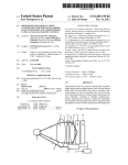
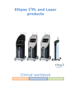
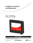
Figure 1-1: Schematic view of a fluoresensor. Different lasers induce
fluorescent light, which is analyzed in the spectrometer and CCD. The results are
displayed and stored on a computer.
The principal components of a fluoresensor capable of induce and collect
fluorescence light can be seen in Figure 1-1. Different lasers are used to induce
fluorescence, and the fluorescence light is collected and analyzed in a spectrometer
and CCD. The transport of light to and from the sample is done in an optical
fiber. The components are further described in section 3.
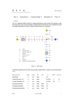
When the planning for the third OMA system started, two similar systems
existed already, similar by means of functionality. The first, presented in 1991 [1],
was constructed on a mobile trolley. It functioned guiding both the excitation
light and fluorescence light through the same optical fiber. The size of the trolley
was about 85x70 ern with a height of approximately 140 em, see Figure l-2a.
The weight was more than one person could handle.
2
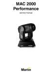
Figure 1-2: Previous systems. To the left (a)the first , to the right (b) the
second.
The second system, presented in 1994 [2], is still in use and has more or
less the same dimensions as the first, but technically improved components, see
Figure 1-2b. Both systems are however difficult to use unless you are a technician,
hard to move without a van and slow to work with since there are several manual
steps involved in the acquisition process.
1.2
Portable and compact system
How small can this type of OMA system be? When the standards for a third
system were set, computer dimensions and optical components size were
considered. A notebook computer with a small docking station was present,
however old and obsolete, wirh an approximate size of 30x40x6 em (wxdxh).
The first calculations of the optical components size aimed at adding only 10 em
to the height and giving a total weight of no more than 20 kg (see Figure 1-3). All
parts mentioned should be bundled into a portable case, small enough to bring as
a hand luggage at any public communication.
3
LUNO
PORTABL~ Ht.OICAL
Fl!Jl)((()SfilSOR.
Figure 1-3: Initial vision of the compact system. Graphics: S Svanberg.
1.3
Intuitive and simple interface
The normal procedure, performing medical investigations with the fluoresensor in
use today, involves at least three persons plus the patient in the room: the
examining doctor, an assistant and a physicist running the equipment. A problem
is the need for the physicist; advanced equipment like these often need advanced
operators, especially when unpredictable events occur.
One goal with the third OMA system is to make it possible for the
examining doctor, or the assistant, to handle the equipment. This demands
automated procedures and easy interaction with the controlling computer. Using
the system in its most simple mode, it could give audio directions, give simple
indications on the characterization of the tissue, and be voice controlled.
The software used with the present systems are general, third-part
applications, constructed only to acquire a spectrum without knowledge about the
situation. A more custom-designed software is welcomed.
1.4 Time-resolved measurements
When specifying the system it was desired to be able to perform time-resolved
measurements. This can be used when monitoring changes in fluorescence light
life-times, which applies to tissue differentiation. Usually, the system gives
intensity as a function of wavelength, but in a time-resolved measurement another
dimension is added; time. The intensity of different wavelengths as a function of
time is of interest. Today's technology should offer this feature, even in compact
4
systems. This option has not been disabled by any included component, though
not yet implemented.
5
2.
Laser-induced fluorescence in tissue
2.1
Introduction to fluorescence
Fluorescence is a process in matter, starting with absorption of photon energy [3],
see Figure 2-1 [4,5]. If an incoming photon has the same energy as the difference
between two electronic states in an atom or molecule, it can be absorbed if the
lower state is occupied. In the atom case, the excited atom returns to the initial
state by emitting a photon, which therefore has the same energy as the absorbed
photon. This is called resonance radiation. In the molecule case, the emitted
photon energy may be less than the absorbed. This happens if the excited
molecule is deexcited to an energy level higher than the original level, or if it
relaxes before emission. This radiation is called fluorescence.
Excited states
>,
CJ)
'QJ
J
c
Ll.J
Ground state
Figure 2-1: Energy level diagram and terminology for radiative processes.
Relaxation is a radiationless process, in which some of the excess molecular
energy is released to the surroundings. The electronic energy states in a molecule
consist of many levels of almost equal energies, forming an energy band. The
many, in energy closely spaced, molecular configurations are due to differences in
7
molecular vibration and rotation. It is within these bands relaxation takes place.
Typical relaxation energies within vibrational bands are of the order of 10·1 eV.
This process is very fast compared with electronic deexcitation, and the energy is
released as heat to the surrounding molecules.
When the electron has reached the lowest level within the energy band, it
eventually is deexcited to a lower electron state. This state can form another band,
in which another relaxation process can take place.
The re~atively wide bands make the exciting wavelength non-critical
within an interval of the order of 10-50 nm for visible light, and gives a continuos
fluorescence distribution ranging over about 100 nm.
2.2
laser-induced fluorescence
The quantum yield for the fluorescence process, i.e. the number of fluorescence
photons emitted divided by the number absorbed, is low for most molecules. The
fluorescence is often weak and broadly distributed, and light propagation in the
medium of interest may be limited. It is thus essential to have a relatively high
power excitation source when performing fluorescence measurements. Laser
excitation is thus often preferable, since a laser delivers outstanding power within
a narrow wavelength band.
Other advantages of lasers as excitation sources are that they are spectrally
clean, and have a high brightness. A single wavelength is critical. The fluorescence
excitation source should emit light at a wavelength absorbed by the molecules
studied but nothing at the wavelength where the fluorescence is analyzed. Any
light emitted by the source at this wavelength will disturb the fluorescence
detection.
A high brightness is also essential to enable efficient guiding of the
excitation light from the source to the sampling volume. Fiber delivering is often
necessary in medical applications.
2.3 Spectrally- and time-resolved laser-induced
fluorescence
In order to enable that fluorescence from different molecules can be distinguished
in the analysis of complex samples, such as tissues containing several fluorescent
molecules, the fluorescence is often resolved spectrally. This means that the
fluorescence intensity is measured as a function of wavelength. This is how the
fluorescence has been analyzed in the old systems at the Division of Atomic
Physics, Lund.
The system described in this thesis utilize this means of distinguishing
contributions from different molecules. However, the new fluorescence system
also employs an additional tool to distinguish fluorescence from different
molecules - it provides fluorescence lifetime information.
Lifetime is by definition the inverse of the probability of deexcitation for a
given transition. The lifetime of fluorescent light can be determined by doing
8
time-resolved measurements, where studying the decay of the fluorescence
intensity from a excited matter.
Normally, a detection time resolution of picoseconds is needed, since
typical fluorescence light lifetimes vary down to nanoseconds or even picoseconds
[3, 6, 7]. However, if achieving the actual lifetime is not necessary but only the
ability to prove presence of a certain matter, nanosecond resolution of the
detection system may be sufficient.
0 ne way to do this is to compare late and early intensity integration of the
fluorescent light. This affords a controlled gating of the detector in means of both
width and delay.
2.4 Tissue fluorescence
Tissue fluorescence origin from numerous fluorophores. Native as well as added
exogenous fluorophores can be utilized for tissue diagnostic purposes. The
fluorophores of diagnostic interest often exhibit absorption in the violet region
and fluorescence in the visible wavelength region.
A commonly used absorption band for tissue fluorescence is the Soret band
of porphyrins, a very strong absorption band in the blue region of the optical
absorption spectrum [5,8]. The corresponding excitation wavelength to the
absorption is 405 nm, which can be obtained with a dye laser. The dye can be
pumped with a nitrogen laser (337 nm) or a frequency-tripled Nd:YAG laser
(355 nm).
The states between which absorption occurs are the ground singlet states
5 0 and 5 2 • Internal conversion relaxation (see Figure 2-2) brings the electron to Sl'
from which it deexcites, emitting a photon of 635 nm or 700 nm, to S0 •
Phosphorescence may also occur, if intersystem crossing brings the electron from S1 to
a triplet T 1 state, and from there deexcites to S0 •
9
>.
0'1
'-
OJ
c
Ll.J
·.;:;
c
0
E
2- c
.
0Vl
..0
<(
LJ1
0
3
(])
u
c(])
u
Ec
u
0
0
u
"E-
(])
c
(])
Vl
(])
.....
0
Vl
c
(])
.....
I.J)
_c
IYl
_c
0
::::l
u:
~
c..
Vl
0
a..
Distance between nuclei
Figure 2-2: Illustration of absorption, internal conversion, intersystem
crossing and phosphorescence in a Pp IX molecule.
2.4.1
Autofluorescence
The fluorescence in tissue depends on many factors, e.g. the type of cells, pH and
the kind of fluorescent substances/molecules - fluorophores. The absorption
spectra of some important tissue molecules can be seen in Figure 2-3. Examples
of tissue fluorophores are collagen, carotene, elastin and NADH [5]. When using
UV light as an excitation source, NADH fluoresces in a bluish color, peaking at
470 nm, while carotene fluoresces around 530 nm. Collagen and elastin have
slightly separated peaks around 400 nm.
The balance between NADH and the less fluorescent NAD. depends on
pH, thus a low pH gives less fluorescence. The natural fluorophores col}tributes to
the native tissue fluorescence - tissue autofluorescence.
10
Figure 2-3: Absorption spectra of tissue chromophores {Graphics: Boulnois).
2.4.2
Fluorescent tumor markers
To perform laser-induced fluorescence (LIF) measurements, one can use
exogenous fluorescent tumor markers. These substances have characteristic
fluorescence emission, and can therefore easily be detected. 0 ne important
fluorescent tumor marker is HpD, a hematoporphyrin derivative.
Hematoporphyrins exist naturally in the body, and HpD is tumor-seeking rhus
useful for cancer diagnostics. A probable reason for the tumor selectivity is that
tumors have weaker barriers between blood circulation and cells, which HpD
normally is too large to enter. One problem with HpD is its instability and its
ability to aggregates [5].
A newer substance among fluorescent tumor markers is ALA,
8-amino levulinic acid. This is a precursor in the heme cycle of the body, and
transforms into protoporphyrin IX, Pp IX. ALA is easy to give to the patient
intravenously, orally or topically and Pp IX has similar fluorescence characteristics
as H pD. An advantage is that ALA itself is not fluorescent, making the given dose
less critical. When used for LIF, the most commonly used excitation wavelength is
405 nm. The major fluorescence peak is at 635 nm, and a minor at 700 nm, see
Figure 2-4 (right).
II
2.5 Medical diagnostics
Since certain fluorescent tumor markers accumulate in tumors, laser-induced
fluorescence can be used to detect cancer [5]. The pH in tumors is often lower
than in normal tissue, thus autofluorescence due to NADH is decreased.
Comparing the peak intensity of the specific fluorescence from the sensitizer with
the bluish autofluorescence makes it possible to distinguish tumors from normal
tissue (see Figure 2-4).
It is also possible to characterize tissue without adding a fluorescent tumor
marker. UV excitation light has shown to give good contrast in the bluish
autofluorescence distribution between tumor and normal surrounding tissue [1].
Using dimensionless scalars, e.g. the ratio between the Pp IX peak
intensity and autofluorescence intensity, gives many advantages compared to using
absolute values. Excitation power dependence, spatial dependence, detection angle
dependence and other factors, are eliminated.
·
Laser-induced characterization have shown high correlation with biopsy
results in for example malignant brain tumors [9], bladder malignancies [1 0], oral
and oropharyngeal tumors [1], colon cancer [11-13] and atherosclerotic plaque
[1,14,15].
Suspected site
x 1Q4
Normal site
7,---~--~--~--~---.
4000
3500
3000
.
~
0
2500
~ 2000
g
3
1500
1000
)
500
300
400
300
400
500
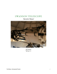
Figure 2-4: Typical spectra from a patient given ALA. The left graph shows a
spectrum from a normal site, a large autofluorescence peak at about 480 nm and a
small Pp IX peak at 635 nm is shown. The right graph shows a spectrum from what is
considered a suspected site. A significantly smaller autofluorescence peak at 480 nm,
and relatively large Pp IX peak at 635 nm. The Pp IX peak at 700 can be dimly seen.
{Backgrounds are subtracted from both graphs.)
A non-LIF method is using a white light source to get an elastic scatter
classification tool. One example is classifying bladder cancer, where elastic scatter
measurements have shown good results [16].
It has been shown that fluorescence light from porphyrins have a longer
effective lifetime than autofluorescence light from tissue at 635 nm [17,18], thus
time-resolved measurements can be used as a tool for tumor differentiation. The
time-resolved method can also be used for detection of atherosclerotic plaque
[19].
12
3.
Hardware
3.1
Introduction
An OMA system for fluorescence measurements has two basic functions: to
provide excitation light, and to detect fluorescence light. In this case the common
substance in which fluorescence appears is tissue and the information in the
fluorescence light can be used to characterize the tissue. Tissue diagnostics
demands motivate the use of three light sources: light for protoporphyrin
excitation, light for autofluorescence excitation and broadband light for
reflectance measurements (see section 0). The collected fluorescence light is
conveniently analyzed in a computer, thus a suitable detector is a computercontrolled CCD (charge coupled device) camera attached to a spectrometer.
An optical fiber is a good transportation medium for excitation and
fluorescence light, and simultaneously an effective probe. Using a fiber raise small
restrictions to accessibility to the area of interest. Using only one fiber for both
delivery of excitation light and collection of fluorescence light is convenient and
provides a reproducible detection geometry, but requires a beamsplitter to
separate outgoing and incoming beam paths (see Figure 3-1).
>380 nm
fluorescence
...
...337 nm
>380 nm
Figure 3-1: The principles of a dichroic beamsplitter. Excitation light, short
wavelength, enters from the right (337 nm) and is mostly transmitted. The fluorescent
light, long wavelength, returns from the left, and is reflected.
The use of a pulsed light source and a gated detector makes it possible to
efficiently suppress ambient background light and thus allows use in normal
daylight. Gating means that the CCD is exposed only when light of interest is
expected, thus shielded from unwanted light.
A major part of this project was to gather information about and order the
different components in the OMA system. Some of the important components,
such as lasers and detector, were already ordered when we entered the project.
13
3.2 light sources
3.2.1
UV laser
UV light at 337 nm has shown to give good contrast in the bluish
autofluorescence distribution between tumor and normal surrounding tissue (see
2.5). A nitrogen (N) laser is thus suitable as an excitation light source, and such a ·
laser (VSL-337, Laser Science) already existed from a previous system at our
disposal.
This is a pulsed laser and currently can be operated at 1-20 Hz, with a
pulse duration and energy of 3 ns and 100 l!J, respectively. The physical
dimensions were originally 117x260x53 mm (wxdxh), but have been slightly
modified to fit the system.
The laser runs on 12 V DC, conveniently fed from the power adapter (see
3.7.2).
3.2.2
Dye laser
A wavelength efficiently matching the Soret band of porphyrins is 405 nm, see
(2.4). This light is produced by pumping a dye laser (DLM220, Laser Science)
with the above mentioned UV laser. The dye laser uses the dye DPS (4,4'Diphenylstilbene), which is fluorescent at 394-416 nm with the peak at 404 nm.
The dye laser tolerates a maximum average power of 0.5 m W, but our setup
produces a pulse energy of 5-10 !!I at 20Hz.
The dye laser also existed in previous systems, thus present when we
entered the project. We had to redirect its beam path (see Figure 3-2) to achieve
the compactness of the system, and remove some excess material.
14
laser before ad·ustment
rror
The dye laser after adjustment
405 nm
337 nm
Figure 3-2: Geometry of the dye laser before and after modification.
3.2.3
White Halogen Tungsten lamp
Often abnormalities in the fluorescence spectra indicate that something is
incorrect with the acquisition, e.g. blood on the fiber tip. The use of a broadband
light source may help troubleshooting by showing low reflectance where
hemoglobin absorbs. Another reason to include a white light source is to get an
elastic scatter classification tool (see 2.5).
15
Spectrum from the broadband halogen lamp
X 105
5 . .----.----.----.----.----.---.----.----.----,
4.5
Light has passed a 385 nm cut-off filter
4
3.5
3
Cll
§
2.5
0
(.)
2
1.5
0.5
400
450
500
550
600
nm
650
700
750
800
850
Figure 3-3: Spectrum from the broadband tungsten halogen lamp, as recorded
by the system. The light has passed a 385 nm cut-off filter because of beta-version
reasons.
A small broadband light source was needed (see Figure 3-3), and after
investigating the market we decided to get a tungsten halogen lamp (LS-1, Ocean
Optics). This lamp gets hot, but is small enough to be placed where heat
production effects are minimized. The lamp is powered by 12 V DC.
3.3 Guiding the light
Minimizing the number of components and the path length were the main
objectives when designing the different beam paths, see Figure 3-4 and Figure
3-6. A large number of optical components increases the complexity of the system
and optical errors. Moreover the light exchange decreases with each surface
passed. The path length is crucial as the beams actually are slightly divergent.
16
~Mirror
.,1;;;:iJ.i>
Flip-in mirror
.:::::::> Beamsplitter
®
Lens
Figure 3-4: Schematic view of the different beam paths.
3.3.1
laser light selector
Switching automatically between N 2 and dye laser is done by a flip-in mirror
(8891M motorized Flipper™, New Focus). It provides fast switching and
supports TTL control from a computer. Good repeatability is another important
feature along with accurate tilt-and-trim adjustment (see Figure 3-5). The mirror
is coated for maximum reflection at 351 nm, as 337 nm was not available.
17
Figure 3-5: Detail of the New Focus motorized Flipper. Tilt-and-trim
adjustment is offered by the allen-keys. This figure shows the flipper that selects
between laser and white light.
The flipper came with a control handpad, which had to be modified for
two reasons. We wanted to arrange with internal power supply instead of battery,
and stripping the handpad cover and button decreased its size.
Guiding the light from the dye laser in an identical beam direction as light
from the N 2 laser, i.e. hitting the same spot from the same incident angle, is
arranged with a mirror, see Figure 3-6. The mirror is coated-for maximum
reflection at 364 nm (405 nm not available), and mounted in a holder with tiltand-trim option (9771M Econo-Mount™, New Focus).
The beam path for 337 nm
The beam path for 405 nm
The beam path for white light
<J7 Mirror
.,{;;.:>Flip-in mirror
-~:::::> Beamsplitter
0 Lens
Figure 3-6: Detail view of each beam path. When a flip-in minor is down, it is
not shown.
3.3.2
Laser beam compression
The beam from the N 2 laser is too wide to fit the optics, thus compressing the
beam is the next step along the way. Two positive fused silica lenses do the job (see
Figure 3-7). Anti-reflective coatings help to keep the intensity up. The mounts
were fabricated by the workshop at the Department of Physics, Lund University.
18
Figure 3-7: Detail of the laser beam compressor.
3.3.3
White light optical fiber
The white light lamp can be placed at a from heat aspects ideal position, since its
light is guided in an optical fiber. The fiber is connected to a fiber port
(FiberPort, OFR) with a collimating lens. The fiber port allows for adjustment in
three dimensions plus tilt and trim. However, the light from the fiber port is
slightly divergent, and since we assume parallel light at next component (see
Figure 3-4), another positive lens collimates the light. This lens is mounted in a
workshop-made lens holder, see (0).
3.3.4
laser versus white light selector
Switching between laser light and white light is, just as laser light selection (see
3.3.1), done automatically by a flip-in mirror, see Figure 3-6 and Figure 3-5. The
mirror is coated for maximum reflection at 364 nm, working well at 337 and
405 nm.
3.3.5
Rotating stage
The main objective of a rotating stage is to match the current light with a correct
dichroic or broadband beamsplitter and cut-off filter. Since a lens adjusting the
beam for the outgoing fiber port has to be on the stage, there has to be three of
them. They have to be on the stage because numerical aperture and beam width
sets the focal length. A minor benefit is that the lenses can have optimized
coatings compared to having one lens for all cases.
19
l
I
I
l
Figure 3-8: Detail of the rotating stage.
The beamsplitters vary in the three different light cases. For the UV
337 nm light, a short wave pass dichroic beamsplitter with a cut-off wavelength at
380 nm is used. The corresponding cut-off wavelength for the 405 nm dye light is
450 nm. The substrate is fused silica. The white light beamsplitter is a broadband
50-50% beamsplitter, working in the interval 488-694 nm, coated on a BK7
substrate. All above mentioned beamsplitters are 1 inch in diameter and mounted
in tilt-and-trim holders (9884MK, New Focus).
The lenses between the beamsplitters and the outgoing fiber port collect
the light to fit the numerical aperture of the fiber port. The anti-reflection
coatings are optimized for the ranges 337-600 nm (UV light), 400-700 nm
(405 nm light) and 400-700 nm (white light). The lenses are mounted in
workshop-made lens holders (see O) since the available space is very limited.
When the fluorescence light enters the system, it is reflected in the
dichroic beamsplitters. To make sure that all excitation light is discriminated, long
pass cut-off filters are glued on the stage. For UV excitation light, the cut-off
wavelength is 385 nm (BG 385, Schott) and for 405 nm dye light the cut-off
wavelength is 435 nm (BG 435, Schott).
To improve the detected signal, plasma lines from the UV laser is not
allowed to exit the system. A laser line interference filter is glued on the rotating
stage, in front of the dichroic beamsplitter used for the 337 nm excitation light.
A close up picture of the optics on the rotating stage can be seen in Figure
3-8.
3.3.6
Optical fiber probe
The light to and from the external fiber is assembled at an OFR fiber port,
identical to the one in section (3.3.3). The fiber port makes it easy to attach a
sterilized optical fiber. The distal end of the fiber is positioned in contact with the
tissue to be investigated. This fiber is made in quartz with a core diameter of 600
flm.
20
3.3.7
Spectrometer lens
Fluorescence light reflected by the beamsplitter is adjusted to be parallel,
using the lenses on the rotating stage. To focus this light to the entrance slit of the
spectrometer and to match its numerical aperture, a positive quartz lens is placed
in front of the slit. The substrate is fused silica to minimize fluorescence in the
lens itself.
Again, a high light throughput is important. The lens is thus mounted in
a workshop-made lens holder, which in turn is placed on a translation stage. This
gives adjustment possibilities in all three dimensions.
3.4 Spectrometer and detector
When we entered the project two different spectrometers were ordered. One
Oriel Instruments MS 125 Spectrograph, and one ISA spectrograph model
CP-140. The advantages with the MS 125 are its physical dimensions and its
external geometry, i.e. the entrance slit is conveniently placed.
The CP-140 is larger and more difficult than the MS 125 to fit into the
system, but has a better numerical aperture and a fixed grating.
The MS 125 arrived first, and we could quickly state its performance as
satisfying. Since we wanted a compact system, a decision to use it was taken. As
we are writing this thesis, the CP-140 has still not arrived, so we think we did the
right thing.
3.4.1
Oriel MS 125 spectrometer
The Oriel Instruments MS 125 spectrograph is a crossed Czerny-Turner
spectrograph with a F/number of3.7 (see Figure 3-9). We are using it with a 100
Jlm slit and a 400 lines/mm ruled grating, blazed for 500 nm. This gives a
of 300-1200 nm and a resolution of 1 nm.
Figure 3-9: Detail of the spectrometer. The thick cable passes safely below the
beam path.
21
3.4.2
Andor lnstaSpec V JCCD detector
Connected to the spectrometer is the detector (InstaSpec V ICCD, Andor
Technology). It consists of a few different components: a detector head with an
image intensified CCD array (see Figure 3-1 0), a PCI card for the computer and
a multi-IO box, used to send ·
and
· signals.
Figure 3-10: The Andor lnstaSpec V ICCD.
The CCD array has the resolution of 1024x128 pixels, where the second
dime'nsion's 128 pixels usually are summed together, binned. The horizontal 1024
pixels give a resolution well matching that of the spectrometer.
To be able to do time-resolved measurements (see 1.4), the image
intensifier can be gated with gating times down to 3 ns. This requires that external
adjustable delay electronics is connected. Normally larger gate times will be used.
An external adjustable delay generator, necessary for short gating times, is bulky
and would considerably increase the size of the system. It is for that reason
excluded in this first compact version of the fluoresensor.
To minimize the acquisition of background light, the multi-IO box (see
Figure 3-11) is custom-designed with a built-in delay function trigged with a
diode, giving a 0-100 ns delay followed by a 20-100 ns gate signal. The trigger
diode is fed from an optical fiber, picking up stray light from the output mirror of
the UV laser. The delay function is used to compensate for the time difference
between the trigger signal and the fluorescence to reach the detector. To catch the
incoming fluorescence we have chosen the delay and gate width to 40 and 100 ns,
respe
22
Figure 3-11: The modified multi-10 box. The optical trigger diode connector
is in the black area to the right.
The detector has a gain of maximum 4500 counts per photoelectron. In
most cases this is too much, resulting in saturation of the CCD. Useful values of
gain have shown to be 30-120 counts per photoelectron.
Cooling the CCD decreases the dark current signal, and this is done in up
to three stages [20]. Our system only use single stage cooling, which requires
additional power supply to the PCI card. This power, 5V DC 5 A, is supposed to
be delivered from the power supply of the computer but the used computer does
not support this feature, so a 5V DC 5A power adapter has been added to the
system (see 3.7.2).
3.5 Computer-controlled components
Switching between different light sources takes a long time in present systems,
especially from a patient's point of view. The components associated with each
light source are dichroic beamsplitters, cut-off filters, mirrors and lenses with
different coatings. All these components had to be replaced, manually one by one.
The system developed now is designed to switch these components automatically,
when possible in parallel, in the new system.
3.5.1
light source control
The UV laser fires when receiving a trigger pulse from the PCI card via the multiIO box. If an acquisition without laser excitation light is desired, the software
makes sure that no trigger pulse is generated. The same procedure is valid in the
dye laser case.
The white light lamp is activated and inactivated by turning on and off
the current through the lamp. A computer-controlled relay does this job.
3.5.2
light selecting flip-in mirrors
The flipper controllers accept TTL signals. They can thus be software controlled
via the parallel port on the computer. Controlling the parallel port on Windows
NT turned out to be quite tricky. \Vindows NT does not allow direct access to
the port itself, as MS-DOS and Windows 95 do. Mter consulting several
"USENET consultants" we found a library to download, including several
functions we could use.
3.5.3
Rotating stage
The rotating stage is motorized via a cog driving belt. The 12 V DC motor is
controlled by the computer, using two functions. Each time we want to turn the
stage one step (120°), a pulse is given on one parallel port pin. The control circuit
of the rotating stage has an optical indicator answering with "high" when the
current position is at a reference position. This indicator is connected to the
parallel port as well.
23
Each time the system starts, or more precisely, when the software starts, it
rotates the stage until the reference position is reached. From there, the software
remembers in which position the stage is, i.e. which set of optics is used.
A springed steel ball ensures that the stage is stopped accurately in exact
positions. Mechanical precision is needed, since the accuracy of the positions
where the motor stops are not sufficient for our purposes.
3.5.4
Detector
Controlling the detector is the most sophisticated task. A wide range of parameters
can be set, all by calls to library functions provided by the detector manufacturer.
Examples of parameters are exposure time and number of accumulations, see Figure
3-12. Commands to the detector are sent in the same way, by calling functions.
Examples of commands are start acquisition, get data and get status.
Figure 3-12: CCD Setup module. Most available detector parameters can be
set. The values are stored in the CcdProps.txt Hle in the library folder.
3.6 Computer
Several demands on the system computer were quite hard to fulfill; it should be
small and light, yet fast and expandable with a PCI card. Most notebook
computers only support PC-card (PCMCIA card), or PCI cards in an external
docking station, often huge and heavy.
24
After a lot of research, we found a company in California, Dolch, who
manufactures a portable computer named FieldPAC [21]. It fulfilled the demands
mentioned above, though quite heavy being a portable, 7.8 kg. However, it is
built into a rugged aluminum attache case, operating in demanding conditions.
It has a nice large 14.1" color display, and standard sound features. Thus
it can provide easy communication with its operator, even at a few meters
distance.
3.7
3. 7.1
Miscellaneous hardware
Base plate
A small yet rigid base for all components in the system is necessary. \Yfe came to
the conclusion to use a strainless plate of aluminum, 10 mm thick. It is now
perforated with mounting holes and completely covered with components.
3.7.2
Power adapter
Two power adapters are needed, one for transformation of 220 V ACto 12 and 9
V DC, and one 220 V AC to 5 V DC. The first serve all mechanics such as
rotating stage motor, flippers, laser and halogen lamp. The second was thrown in
at a late stage to provide power to cool the CCD. This power was expected to be
taken from a more conventional computer, but not supported by the FieldPAC.
25
4.
Software
4.1
Introduction
Since the OMA system should allow tCl be maneuvered by a non-specialist, e.g. a
physician, a simple graphical user interface is required. Additionally, the software
-must be possible to upgrade and further develop, thus understandable and
structured. The commercial applications of today has a physicist's approach,
which makes knowledge about parameters and procedures necessary. These
applications give a good detail control, a mandatory part even in our application,
but some parts can be greatly simplified.
The Division of Atomic Physics expressed a wish that we should develop
the software in Lab VIEW, a graphical development environment from National
Instruments, made for instrument control and data acquisitions. This would itself
provide for maintainability and a low step-in level when learning to modify the
application.
4.2
Control the acquisition process
To make a correct acquisition, one must follow some necessary steps in a certain
order. The detector parameters must be set, the light sources should be triggered
and then the detected information can be collected and stored.
Andor distributed the detector system with software drivers, including
functions controlling all aspects of the camera, and examples using these functions
in a few different programming languages. Andor also provided a programmer's
guide [22], explaining the functions and suggested order of usage (see Figure 4-1).
27
Initialize
detector
--
Setup
acquisition
parameters
Monitor
temperature
Start
acquisition
Yes
Monitor
acquisition
Get
acquired data
Switch off
cooler
Monitor
temperature
Close down
detector
Figure 4-1: Block diagram of the acquisition process. An acquisition should
not be performed before the temperature has stabilized at desired level, and the system
should not be shut down before the temperature is above 0°C.
We implemented these functions and rules into what we call "Andor
Boxes", e.g. SetupAcquisitionParameters, StartAcquisition and GetData. Some
simple functions were implemented too, for instance SwitchCoolerOff, for
reasons of consistency. An example of the use of these boxes can be seen in Figure
4-2.
28
,
........................................................
:
~
tne~
l:.f............f> . -...lQj
Figure 4-2: This diagram shows the use of some Andor boxes. A typical
real-time acquisition is done, initialized with the Start Acq.-box. Get Data reads the
spectrum, and if not Done is pressed, the succeeding acquisition starts. While the
succeeding acquisition is exposed, the previous is displayed.
Selecting the excitation light source is divided in different layers. The top layer is a
VI (Virtual Instrument) called SetLight, which simply requires a parameter 0-2,
indicating which source to use. Inside this VI, there is an abstract component
layer, which consists of VIs for each motorized component. Depending on the
desired light source, the flippers and the rotating stage must be given signals.
These VIs also return estimated values of the time required to change state.
SetLight itself returns the largest of these values, see Figure 4-3.
Figure 4-3: A view from SetLight.vi's diagram. The frame shows what is done
when selecting white light as an excitation source. Flipper number one is not changed,
while Hipper number two is down (false). The rotating stage is in position 2 {0-2).
Each component returns an estimated time needed to fulftl.l the request, and the
maximum time is considered.
29
I
The abstract component VIs change the states of the corresponding parallel port
pins, or as in the rotating stage case, generate a short pulse on a pin. As mentioned
in section (3.5.2), controlling the parallel port in Windows NT is not
implemented in Lab VIE\X!, but Scientific Software Tools provided a DLL
(dynamic link libra1y) we could download. This library has functions we could
call from Lab VIEW, changing the state of the parallel port.
4.3
Analysis of acquired information
The purpose of the OMA system is to provide data for classification. Signal
processing is therefore an important issue, just as it is important to save the raw
data for later external analysis.
4.3.1
Wavelength calibration of the detector system
To be able to relate a pixel number (channel) on the CCD to a specific
wavelength, a calibration must be performed, at least once. Since the grating of
the spectrometer is locked in position the wavelength calibration should be fixed,
but new calibration spectra will probably be acquired at each measurement
session.
To achieve precision in the calibration, light sources with sharp and well
determined lines should be used. Fortunately, an ordinary fluorescent light tube
fulfills these requirements, since its mercury lines are apparent and known with a
resolution far better than most of the system.
To make this process easy, even automatic, we have implemented a
library, in which known calibration sources can be stored. Once and for all, the
peaks of a source can be defined with desired precision. When given a sample, the
system picks the most similar library spectrum, and relates the peak wavelengths
from the libra1y with the detected peak channels in the sample. The method used
to pick the most similar libra1y spectrum is cross-correlation [23]. Optionally, the
system gives an audio confirmation of the calibration.
The result of the calibration is a linear function determined by a least
squares fit, giving slope and intercept values. These values are stored and used in
future acquisitions.
4.3.2
Intensity calibration of the detector system
The sensitivity of the detector system is not uniform at all wavelengths, thus an
acquisition of a light source with a well-known intensity distribution must be
performed. All following acquisitions can be compensated for the hereby known
irregularities.
4.3.3
Processing
Some data processing is done automatically or optionally. A background
acquisition can be subtracted to remove fiber fluorescence, surrounding light and
30
I
l
dark current effects (see 3.4.2), all to display a more true result on the screen as
well as to provide better data for analysis.
4.3.4
Data storage
All acquired spectra are saved to disk. A text-based file format containing most
parameters is used, e.g. if a background is subtracted, a note about which
background subtracted is attached. It is necessary to save all data for a proper
statistical evaluation.
4.3.5
Fast analysis
It is possible to design a criterion which can be used in real-time to do a fast
analysis of a spectrum. A parameter in the criterion could be the intensity over a
certain wavelength interval, and ratios can be formed for different intervals.
Figure 4-4 shows the design of a criterion, and Figure 4-6 the use of the same
criterion in an examination situation.
Figure 4-4: The Criteria Editor module. Here a criterion called "ALA" is
shown. The expression uses three variables, and below the expression the definition of
the variable "fluoroPeak'' can be seen.
31
A simple cancer criterion could be
fluoroPeak
::__
______.-. ._jluoroBase
. . : :_____ + 0.5 > 2
· jluoroAuto
jluoroPeak = /(635)
fluoroBase
= 1(600)
jluoroAuto = 1(500)
which compares the intensity of the protoporphyrin fluorescence with the autofluorescence intensity and can be used to classify skin tumors as described in
section (2.5). One way to present the result is a red and green lamp, where red
corresponds to a fulfilled criterion, see Figure 4-6.
4.4 Technical structure of the software
One important issue when we designed the structure of the software was to make
it easy to add new functions and interfaces. For instance, if large-scale
examinations are planned, a tailor-made sequence of functions and interfaces may
be preferred.
4.4.1
Modular implementation
We have striven for making it easy to combine elementary functions into larger
tasks or sequences. The concept module developed, which is a VI that can be
called from a menu, put in a sequence or put in a loop structure. A module must
take certain parameters, and return some specified values. Examples of modules
are Calibrate, CCD setup and, actually, Advanced menu which is an application of
the Select module.
Inter-module communication is supported via so called properties, which
are variants of global variables. This is necessary, since the parameters to and from
a module are fixed.
4.4.2
Client-server design
After a few weeks of the software development process, we wanted to separate
hardware communication from user interaction. This separation made it possible
to simulate the hardware, which was essential since the hardware has been absent
during most of the development period. The separation also led to that we could
develop the two parts independently, and sometimes in parallel on different
computers. An intellectual advantage can also be motivated with a more distinct
layer design, making it easier to grasp a certain function.
When structuring the new design, we found no reason against making it a
client-server application. This means that the user interacts with a client,
communicating in some way with a server, controlling the hardware. The
32
communication between client and server can be made general, and as in most
cases, over the Internet if the client and server are run on different computers.
Running the client and server on different machines rise new interesting
possibilities. The user can be an expert anywhere, not necessarily in the same
room or country as where the examination takes place. If the acquisition is made
in an environment not suitable for humans, the control staff can be at a friendlier
location. In the medical case, this is known as telemedicine.
Multiple clients is another feature of the client-server design, where one
client probably should act as master client, and the others as observers.
4.5
User interface
The target groups for this application vary a lot in what they want to achieve and
what they know about the different issues involved in the OMA system. A
physician probably wants to use the system as a tool for diagnostics, while a
physicist wants to use it for acquiring pure spectral information.
We have approached this problem by developing multiple sets of modules,
primarily performing the same tasks, but with different interfaces showing either
all available or only essential information. The standard, or simple, modules can
be reached directly from the Main Menu, while the more advanced modules can
be found under the Advanced Menu, see Figure 4-5. No difficult steps must be
afforded to reach standard modules, thus no Standard Menu.
Figure 4-5: The Main menu. Standard modules or sequences can be ron from
here, while advanced or personalized modules are found under respective sub menu.
33
4.5.1
Standard mode
With standard mode, we refer to using the modules with only essential interface
components. These modules are designed to hide all technical and most physical
aspects, and act as automatically as possible. Examples of standard mode modules
are Calibrate and RedGreen.
Figure 4-6: View from the standard module RedGreen.
The module Calibrate performs a calibration (see 4.3.1) by first asking the
user to aim the fiber at an available calibration light source, and then repeatedly
makes acquisitions and compares each one with the library spectra until a match is
found. The module simply terminates by declaring, in text and audio, which
library spectrum it used for the calibration.
RedGreen is a module using "fast analysis" (see 4.3.5) to do a preliminary
diagnose using a selected criterion. The user can only select between continuous
and single acquisition, and select which criterion to be used, see Figure 4-6. The
result is simply displayed with a red or green lamp combined with an associated
sound, for effective communication if the user is alone or visually occupied.
4.5.2
Advanced mode
In the advanced mode modules we try to give the user maximum control and
feedback, so that the desired task can be carried out. All settings that can be
adjusted are available, and original terms are used such as Full vertical binning and
Kinetic cycle time which are terms about detector settings.
Advanced mode also covers modules used to configure the system and the
application itself. Examples are the Edit Initialization File module, in which
menus and sequences can be designed (see Figure 4-7), and CCD setup, which is
34
used to configure the detector. More information about the application
customization can be found in Appendix A.
criteria. vi
Deletelibr aryS pectr a. vi
editlniFile_vi
enterAdvanced.vi
homFile Tolast vi
leavet..dvanced. vi
processSpectrum ToCalculated. vi
select IniFile. vi
selectlibrarySpeclrum. vi
serverCmd. vi
Figure 4-7: Edit Initialization File module. This module is used to build
menus and sequences. The list box to the left shows the modules in the advanced
library, from which modules can be selected and inserted into the Sequence list box.
For each entry in the Sequence list box there is Associated information, e.g. the menu
item displayed.
4.5.3
Personalization
Embedded modules for changing the appearance of menus and sequences provide
for customization. A user can define a personal set of modules and list them in a
new, separate menu. Tailor-made modes can be developed, where personal
opinions about user interface and interaction can be considered, or where taskspecific modules can be bundled. An example of personal menus can be seen m
Figure 4-8.
Figure 4-8: Example of a personalized menu.
35
5.
Evaluation
The OMA system was tested in a campaign of in vivo measurements of the
human colon at the Karolinska Hospital in Stockholm. In the campaign LIF
spectra was collected from normal colonic and rectal tissue and various tissue
polyps which may occur in the colon or the rectum.
Polyps in the colon are typically 1-10 mm in diameter and have
approximately the same light-red color- as the normal colonic tissue, and can
roughly be divided into adenomatous and hyperplastic po!Jps. The adenomatous
polyps are considered precancerous, while the hyperplastic polyps are considered
harmless. To prevent future cancer, polyps are removed from the colon during
colonoscopy. The decision which polyps to remove is made by the endoscopist
from visual impression since adenomatous polyps generally are darker red than the
hyperplastic polyps, but this method is inaccurate even for experienced
endoscopists. Studies have shown considerable difference between the polyp
classifications of an endoscopist and a pathologist [24]. Therefore biopsies are
taken from all polyps found during colonoscopy. Picture of a polyp can be seen in
Figure 5-1.
37
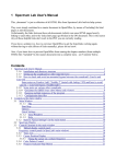
Figure 5-l: A polyp seen from the endoscope. The tip of the fiber is
approximately 0.6 mm in diameter.
Laser-induced fluorescence is a promising approach to a tool for the
differentiation between adenomatous and hyperplastic polyps. Previous
investigations indicate that autofluorescence from adenomatous polyps has
similarities to autofluorescence from malignant tumors [11,12]. It has also been
shown that ALA can be used to distinguish adenomatous polyps from normal
tissue [ 13]. The purpose of the campaign at the Karolinska Hospital was to collect
enough LIF spectra from adenomatous and hyperplastic polyps to evaluate the
possibilities to differentiate between these.
LIF spectra was collected during colonoscopy, in which an endoscope is
used to view the inside of the colon. The endoscope is up to 170 em long to reach
the entire colon, and the tip of the endoscope is maneuverable from outside to
make it possible to guide the endoscope up through the colon and to make
navigation easier. The tip of the endoscope is also equipped with lighting, a video
camera and a system for cleaning the camera lens. The video signal is transported
to an external screen which can be viewed by the examining endoscopist. The
endoscope is also equipped with a channel for accessory instruments, such as
38
biopsy tongs. The fiber probe of the OMA system was inserted into an open
channel, and lead through this channel to the area of interest. Pictures of the fiber
probe in the colon can be seen in Figure 5-2.
Figure 5-2: Acquisition from lumen and fro'in a normal site.
Fluorescence measurements were made with the two supported laser
wavelengths 337 nm and 405 nm. All polyps found during the examination and
some normal area of the colon was investigated with LIF. Measurements were
made in contact with the tissue to optimize the collection of fluorescence and to
obtain a reproducible measurement geometry. Each acquisition consisted of 60
excitation pulses fired at 15 Hz.
Since fluorescence and stray light from the detection system itself and the
background light in the colon should be subtracted from collected data,
background acquisitions for each excitation wavelength were taken in the free
space within the colon lumen. New background acquisitions were taken for each
new measurement area.
Six endoscopists examined 79 patients in three investigation rooms and
about half of the patients had been given ALA orally at least two hours before the
examination. One hundred and seven (1 07) polyps and *** normal sites were
measured. Typical spectra from the campaign can be viewed in Figure 5-3 to
Figure 5-7.
39
Figure 5-3: Acquisition from a normal site. Only autofluorescence is detected.
This is a view from the program used at the study at the Karolinska Hospital,
Stockholm.
Nonnal
X 104
1
(337 nm)
~
~
10
~
s~e
6
0
300
350
400
450
500
650
700
750
BOO
650
700
750
BOO
nm
3
X
Suspected site (337 nm}
104
2.5
§1.5
.(
0.5
0
300
!\'
350
J
400
450
500
'
550
600
Figure 5-4: 337 nm spectra from a non-ALA patient. The upper spectrum is
from a normal site, and the lower is from a suspected adenomatous polyp. Note the
slope difference at about 400 nm, which is steeper in the normal case.
40
Normal
s~e
(405 nm)
-E4
5
0
3
300
35D
400
45D
55<)
5DO
750
700
800
nm
Suspected site (405 nm)
10000
8000
.
I
'\
6000
4000
2000
~
~1\~f:<:l"'~
.·
300
35D
400
450
II
~~""'
500
55D
600
~
650
700
750
800
Figure 5-5: 405 nm. The upper spectrum is from a normal site, and the lower
is from a suspected adenomatous polyp (same as in Figure 5-5). The peak at 635 nm is
significant.
X
Normal site (337 nm)
104
12
~~~
10
/~
i
0
300
350
400
450
500
55<)
600
650
700
750
800
600
650
700
750
800
nm
X
15
Suspected site (337 nm)
104
10
~
0
300
350
400
450
5<)0
55<)
Figure 5-6: 337 nm spectra from a non-ALA patient. The upper spectrum is
from a normal site, and the lower is from a suspected hyperplastic polyp. Note that no
significant slope can be detected at 400 nm, compared to Figure 5-4.
41
9
Noonal site (405 nm)
X 104
6
"'5
c
§4
2
0
300
9
350
400
450
500
550
nm
600
700
750
600
700
750
600
Suspected site (405 nm)
X104
8
6
c"' 5
54
u
2
0
300
350
400
450
500
550
600
650
nm
Figure 5-7: 405 run spectra from a non-ALA patient. The upper spectrum is
from a normal site, and the lower is from a suspected hyperplastic polyp {same as in
Figure 5-6). No significant peak at 635 run can he detected.
The overall performance of the new OMA system was clearly adequate for
measurements of the colon in a campaign of this extent. Especially the
compactness and the speed of excitation light selections were appreciated by the
endoscopists and the assisting staff. The measurement speed is essential since
colonoscopy are sometimes vety painful for the patient, and it can be very difficult
to keep the fiber in contact with small polyps, due to bowel movements.
We found that the wavelength calibration of the system was steady
throughout the campaign. New calibration spectra acquisitions will probably not
be necessary to take on a daily basis.
Some weaknesses in the design of the system were observed. The trigger
function of the white light source was not working properly so no white light
spectra were acquired. Since the main purpose of the white light source is to
detect abnormalities in the acquired fluorescence spectra this weakness was not
crucial to the campaign. The system operator was responsible to discover
abnormal acquisitions.
The dichroic beamsplitters were not functioning as expected and were
replaced by neutral density beamsplitters. The light intensity loss in neutral
density beamsplitters is 50% for each passage, which means that 75% (1-0.5x0.5)
of the intensity was lost only in the beamsplitters. A dichroic beamsplitter is
designed to preserve no less than 90% of the interesting intensity at each passage,
which means that no more than 20% should be lost in the beamsplitters.
42
Correcting this problem should make the OMA system at least 3 times more
sensitive to f1uorescence light.
Another weakness in the system \Vas that some periodic maintenance work
had to be done. The dye laser beam path had to be realigned due to the
transportation of the system between the three investigation rooms. This was done
twice during the two weeks of the campaign. Also the rotating stage had to be
maintained since the springed ball which ensures that the stage is stopped in exact
positions was grinding brass chips from the stop heels on the stage. These chips
periodically clog the ball's socket. The ball was cleaned and greased once during
the campaign.
43
6.
Discussion
6.1
Results
The system of today's date has several improvements to the previous ones. The
total weight, including the 7.8 kg computer, is 26.8 kg, compared to the previous
which could not be lifted by one man. The size, including an aluminum hood, is
47x40x21 em (see Figure 6-1), significantly smaller than 85x70x140 em.
Figure 6-1: The optical side of the system seen from above.
Despite the fact of great intensity loss in the beamsplitters, the signal
performance is still better than the older systems, according to senior physicists.
The gain on the intensifier was set to 6 out of 9 when acquiring the colonoscopy
spectra, corresponding to an amplification of 115 out of 4583 counts per
photoelectron [20]. Reference measurements were acquired at gain 4 (37
counts/ photoelectron).
Changing the optics for the different light sources takes about a second in
the worst case. This is also much better than in previous systems, where manual
changes took about 20 seconds. The fact that it is controlled automatically by the
software makes the process even faster and is not forgotten by mistake. The
accumulation frequency can be raised to a maximum of 20 Hz, where 10 Hz
seems to be a comparable value in older systems.
45
The software, especially the tailor-made modules, improves the acquisition
procedure by supporting file handling and structured storage of the data. The
operator's effort is reduced to pressing a single button for each acquisition.
6.2
Future improvements of the system
The campaign at the Karolinska Hospital awakened many ideas to improve the
system, and was essential to the evaluation process. The system was occasionally
run by one person alone, and that indicated which tasks that should be scheduled
to the computer.
6.2.1
Ensuring correct position of the rotating stage
After two weeks of intensive use, the rotating stage needed some adjustments. A
small screw fixing the stage to the cog belt axis got loose, and needed to be
tightened. Drilling a small slot for the screw in the axis may solve this problem.
Adding a third optical position indicator notifying that an exact position
has been reached is also desired. If the computer cannot read this signal, it could
simply order the stage to turn one additional revolution, and probably stop in a
correct position.
Small brass chips from the stop heels could be found on the springed ball,
and replacing the heels with ones made in hardened steel should prevent clogging.
6.2.2
A reliable mounting of the optical trigger fiber
The optical trigger fiber telling the multi-10 box when the excitation light
actually is delivered, was mounted into the system at a very late stage. A
temporary holder, made by tape and cardboard, gave a, though unreliable but
working, fixation of the fiber.
A tiny fiber positioner (New Focus 9016M) mounted on a rigid pedestal
is probably a solution.
6.2.3
Improving the performance of the beamsplitters
When testing the optical functionality of the components, the dichroic
beamsplitters showed poor performance reflecting the long wave fluorescent light.
The market was investigated once again for better beamsplitters without result. It
is actually difficult to manufacture short pass beamsplitters with a broad reflection
band.
The solution is changing the setup to long wave pass beam splitting, where
suitable dichroic beamsplitters exist, for instance in previous systems. This
probably means a new base plate, and perhaps some new optics such as lenses with
different focal lengths.
6.2.4
A ventilation system
Several of the powered components produce heat, especially the halogen light
source. Since the detector is cooled to produce less dark current, a low work
46
temperature is preferred. During the evaluation measurements, the temperature
inside the system case raised to approximately 30° C, although the halogen lamp
was not used. A ventilation system with a fan should be considered to lower the
work temperature of the system.
6.2.5
Software improvements
Tailor-made modules for different applications than colonoscopy is desired. The
system is planned to go to London in the beginning of 1999, where it is going to
be used in heart surgery. A search-mode module with sound feedback is probably
a user-friendly interface.
A monitoring client is not yet developed, useful when having an expert
connected from a different location. The main stability of the client-server
structure needs to be improved.
A general-purpose application, similar to AndorMCD, capable of firing
the laser is a must. A simple modification of a small light source control program
is enough if run in parallel with AndorMCD.
A criterion specification that can handle vector variables, allowing for
multivariate linear regression would give instantaneous high-performance
evaluation of spectra.
47
7.
References
1. S. Andersson~ Engels, A. Elner, J. Johansson, S.-E. Karlsson, L.G. Salford, L.-G.
Stromblad, K. Svanberg and S. Svanberg, Clinical recording oflaser-induced
fluorescence spectra for evaluation of tumour demarcation feasibility in selected
clinical specialities, Lasers Med. Sci. 6, 415-424 {1991).
2. W. Alian, S. Andersson-Engels, K. Svanberg and S. Svanberg, Laser-induced
fluorescence studies of meso-tetra(hydroxyphenyl)chlorin in malignant and normal
tissues in rat, Br.j. Cancer70, 880-885 (1994).
3. S. Svanberg, Atomic and molecular spectroscopy, (Springer Verlag, Heidelberg,
Germany, 1992).
4. J. Johansson, Fluorescence spectroscopy for medical and environmental diagnostics,
Dissertation thesis, Lund Institute ofTechnology, Lund, Sweden {1993).
5.
R. Berg, Laser-based cancer diagnostics and therapy- Tissue optics considerations,
Dissertation thesis, Lund Institute ofTechnology, Lund, Sweden {1995).
6. M. Yamashita, M. Nomura, S. Kobayashi, T. Sato and K. Aizawa, Picosecond timeresolved fluorescence spectroscopy of hematoporphyrin derivative, IEEE]. Quant.
Electr. QE-20, 1363-1369 {1984).
7.
H. Schneckenburger, K. Konig, K. Kunzi-Rapp, C. Westphal-Frosch and A. Ruck,
Time-resolved in-vivo fluorescence of photosensitizing porphyrins,]. Photochem.
Photobiol. B 21, 143-147 {1993).
8. S. Andersson-Engels, Laser-induced fluorescence for medical diagnostics,
Dissertation thesis, Lund Institute ofTechnology, Lund, Sweden {1989).
9. S. Andersson-Engels, J. Johansson, U. Stenram, K. Svanberg and S. Svanberg,
Malignant tumor and atherosclerotic plaque diagnosis using laser-induced
fluorescence, IEEE]. Quant. Electr. 26,2207-2217 {1990).
10. L. Baert, R. Berg, B. van Damme, M.A. D'Hallewin, J. Johansson, K. Svanberg and
S. Svanberg, Clinical fluorescence diagnosis of human bladder carcinoma following
low-dose Photofrin injection, Urology41, 322-330 {1993).
11. K.T. Schomacker, J.K. Frisoli, C.C. Compton, T.J. Flotte, J.M. Richter, N.S.
Nishioka and T.F. Deutsch, Ultraviolet laser-induced fluorescence of colonic tissue:
Basic biology and diagnostic potential, Lasers Surg. Med. 12, 63-78 {1992).
12.
R.M. Cothren, R. Richards-Kortum, M.V. Sivak, M. Fitzmaurice, R.P. Rava, G.A.
Boyce, M. Doxtader, R. Blackman, T.B. Ivane, G.B. Hayes, M.S. Feld and R.E.
Petras, Gastrointestinal tissue diagnosis by laser-induced fluorescence spectroscopy
at endoscopy, Gastrointest. Endosc. 36, 105-111 {1990).
13.
C. Eker, S. Montan, E. Jaramillo, K. Koizumi, C. Rubio, S. Andersson-Engels, K.
Svanberg, S. Svanberg and P. Slezak, Clinical spectral characterization of colonic
49
mucosal lesions using autofluorescence and 8-aminolevulinic acid sensitization, Gut,
(1998). (In press}.
14.
P.S. Andersson, A. Gustafson, U. Stenram, K. Svanberg and S. Svanberg, Diagnosis
of arterial atherosclerosis using laser-induced fluorescence, Lasers Med. Sci. 2, 261266 (1987}.
15. S. Andersson-Engels, A. Gustafson, J. Johansson, U. Stenram, K. Svanberg and S.
Svanberg, Laser-induced fluorescence used in localizing atherosclerotic lesions,
LasersMed. Sci.4, 171-181 (1989).
16. J.R. Mourant, I.J. Bigio,J. Boyer, R.L. Conn, T.Johnsonand T. Shimada,
Spectroscopic diagnosis of bladder cancer with elastic light scattering, Lasers Surg.
Med. 17, 350-357 (1995).
17. S. Andersson-Engels, R. Berg, O.Jarlman,J.Johansson, K. Svanbergand S.
Svanberg, Time-resolved spectroscopy for medical diagnostics, CLEO'!JO, Anaheim,
California, 1990.
18. R. Cubeddu, P. Taroni and G. Valentini, Time-gated imaging system for tumor
diagnosis, Opt. Eng. 32, 320-325 (1993).
19. S. Andersson-Engels, J. Johansson, K. Svanberg and S. Svanberg, Fluorescence
diagnosis and photochemical treatment of diseased tissue using lasers: Part II, Anal.
Chem. 62, 19-27 (1990). Invited paper.
20. Andor Technology, ICCD User's Guide, (1998).
21.
Dolch Computer Systems Inc.. Dolch- FieldPAC Data Sheet.
http:l/www.dolch.com/portables/fieldpacdata.html. 1998. Dolch Computer
Systems Inc. 98.
22. Andor Technology, A Programmer's Guide to lnstaSpec Drivers, Programmer's
Guide, (1998).
23.
R.C. Gonzalez and R.E. Woods, Digital Image Processing, (Addison-Wesley
Publishing Company, 1992).
24.
0. Kr()nborg and E. Hage, Hyperplasia or neoplasia. Macroscopic versus
microscopic appearance of colo rectal polyps, Scand.]. Gastroenterol. 20, 512-515
(1985).
25. Melles Griot, Melles Griot 1997-98, (1997).
26.
0. Svelto, Principles ofLasers, (Plenum Publishing Corporation, New York, 1989).
50
8.
Acknowledgments
The authors of this thesis would like to thank:
Stefan Andersson-Engels, our mentor, know-how and support.
Ake Bergquist, always professional and helpful.
Charlotta Eker, you trusted us when giving an opportunity to test-run the system
in real life, and were a very nice company and boss at Karolinska.
Claes af Klinteberg, never far away with advice and help.
NUTEK, Swedish National Board for Industrial and Technical Development, for
the financial support that made this project possible.
Goran Werner, you actually built this amazingly compact instrument.
51
9.
Glossary
binning
when reading the CCD, different pixels (often all pixels in
the same column) can be added and read as one value. This
makes the array act as a one-dimensional vector. Less noise is
another benefit, since a single readout adds less noise than
multiple readouts [20].
BK7
A substrate used in common glass lenses [25].
CCD
Charge Coupled Device. Image area used in detector camera,
commercial video cameras etc. [20]. Silicon-based
semiconductor chip.
dark current
The CCD has always a dark current varymg with
temperature, resulting in noise [20].
DLL
Dynamic Link Library, a Windows function library format.
fused silica
A synthetic substrate used in lenses, which operates in the
UV and visible range [25]. Has a low internal fluorescence.
internal conversion
A radiationless singlet-singlet transition where energy is
transferred via collisions to a change in rotational or
vibrational state.
intersystem crossing
A normally spin-forbidden singlet-triplet radiationless decay
caused by collisions [26].
phosphorescence
Radiation emitted from an intersystem crossing decay.
Significantly longer life time than in fluorescence [26].
photoelectron
The image intensifier of the CCD detector is based on the
photo-electric effect. Each incident photon generates a
photoelectron, which is accelerated and multiplied in a high
voltage electric field.
TTL
Transistor-transistor logic. A digital
communication with 4-5 V signals.
VI
Virtual Instrument,.~ a Lab VIEW concept similar with
subroutine
53
circuit
type
for
10. Index
HpD, 11
A
ALA, 11
autofluorescence, 10
ICCD. See CCD
intersystem crossing,9
B
L
background, 30
beamsplitter, 13, 20, 42, 46
broadband light, 15
LabVIEW, 27
laser, 14
dye, 14
N2, 14
nitrogen, 14
LIF, 11
c
calibration, 30
CCD, 22
client-server, 32
criterion, 31
cross-correlation, 30
Czerny-Turner, 21
M
mode
advanced, 34
standard, 34
module, 32
D
N
delay generator, 22
detector gain, 23
NAD·, 10
NADH, 10, 12
E
0
energy band, 7
excitation light, 13
OMA, 1
optical fiber, 13
F
p
fast analysis, 31
flipper, 17
fluorescence, 7
fluorescent tumor marker, 11, 12
fluorophores, 10
phosphorescence, 9
property, 32
protoporphyrin, 11
R
G
relaxation, 7
resonance radiation, 7
rotating stage, 19, 23
gating, 22
H
s
hematoporphyrin, 11
derivative, 11
software, 27
55
u
Sorer band, 9
spectrometer, 21
user interface, 33
T
w
relemedicine, 33
workshop, 18
56
Appendix A: User's manual
Table of Contents
Modularization .........................-.......................................................... 57
Connectors on a module ........................................................................ 57
Module storage ...................................................................................... 58
2
Modules of certain interest .................................................................. 58
Colonoscopy module ............................................................................. 58
Edit criteria library ................................................................................. 59
3
Strange things ..................................................................................... 60
4
How to .............................................................................................. 61
Add a calibration spectrum to library ...................................................... 61
Build the Client Application ................................................................... 61
Build the Server Application ................................................................... 63
Repair an Initialization file ..................................................................... 63
1 Modularization
Module is a name we use on a VI that behaves in a certain way, good enough to
be a menu entry.
Connectors on a module
A module must have four input parameters; Input index, Sequence size, ini
fileName and Info input. There must be two output parameters, named Output
index and e1Tor out.
Input index
The Input index indicates which item the module is in the current sequence. For
example, if a sequence consists of the modules A, B and C, module B's Input
index will be 2~ This input helps to decide the appearance of the navigation
buttons Back, Next/Finish and Close. For example, if input index is 1, Back will be
disabled.
The Lab VIEW data type is 132.
Sequence size
The Sequence size indicates the length of the current sequence. In the example
mentioned in section Input index Sequence size would be 3. This input helps to
decide the appearance of the navigation buttons Back, Next/Finish and Close. For
example, if Input index equals Sequence size, Next/Finish is labeled Finish.
The LabVIEW data type is 132.
57
ini fileName
The ini fileName is used if the module will read an initialization file. If so, the file
name will be passed here as a string, ABC.
Info input
The info input parameter is free to use as desired. The parameter is set in the
Additional info string field in the Edit Initialization File module. Data type: ABC.
Output index
The Output index indicates how the user decided to end the module. If
Next/Finish was pressed, Output index is Input index plus 1, and if Back was
pressed, Input index minus 1. Zero indicates that Close was pressed. Data type:
132.
error out
If an error occurs m the module, it can be reported through the error out
parameter.
Module storage
Since the application is constructed with different modes in mind, the localization
of the modules is important. Three libraries are currently used to store modules;
standard.llb, advanced.llb
2 Modules of certain interest
Colonoscopy module
This module is made especially to automate the acquisition process at a
colonoscopy examination. It saves all spectra in a structured way, ordered by
patient, area in the colon, and point at each area. It automatically acquires spectra
for each checked wavelength.
58
Figure 10-1: Colonoscopy module, seen with spectra from the lumen acquired.
The bluish plot is fluorescence from 337 nm excitation light {mostly
autofluorescence), and the more violet plot is from 405 nm excitation light. The two
protoporphyrin peaks at approximately 635 and 700 nm can be seen.
The 337 and 405 nm spectra are shown simultaneously in the same graph with
different plot colors. It seemed that the rotating stage could became a bit "cold",
thus an "exercise" button was implemented.
Edit criteria library
You use this VI when you want to create a new criteria, or change an ex1stmg
criteria. A criteria is used to determine if a certain condition is met or not, e.g. if a
spectrum from skin might indicate abnormalities.
59
Existing criteria can be modified by first selecting them in the Select a criteria
menu. Examples of expressions:
(fluoroPeak-fluoroBase)/fluoroAuto + 0.5
(365.32-248)*(3294.44+ 1.23e-3)
All variables used must be defined in the lower part of this dialog. The expression
interpreter is case sensitive.
3 Strange things
Module calibrate.vi in Standard library can be allowed to ignore doing the
calibration if the Description field passed along equals "ignore" and a calibration
already is performed.
60
4 How to ...
With this chapter we will try to answer questions about or explain the procedure
to build the applications, Client and Server.
Add a calibration spectrum to library
It is also possible to associate a wave sound clip with a certain spectrum. Why not
let the computer tell the user which library spectrum it used to do the calibration?
Adding an appropriate sound clip to the sound folder, with the same name as the
description of the spectrum, makes the thing. Example: The spectrum named
"Lysror i A105" is associated with the wave file "Lysror i A105.wav".
Build the Client Application
All VIs used must be saved in the distribution in some way. Depending on
whether the VIs are modules (see Modularization) or not, they should be placed
in Advanced/Standard/Tools or General library.
All new or changed modules should be added to one of the libraries
Standard or Advanced. Since the sub VIs they use must be saved as well, Save with
Options should be carried out. These sub VIs are most likely not modules
themselves, and should thus be placed in General library. Save with Options
prompts you to enter this library, and if Application Distribution is selected, all VIs
are saved without their diagrams.
61
Figure 10-2: Example of a fake VI. This was from an early stage of the Client
development.
Getting this job done for a large application can be a lot of work. It is
therefore suggested that you place all modules used by the program in a fake VI.
Now Lab VIEW can build a tree of the statically used sub VIs and save all of them
in one single Save with Options to General. This means that the modules, and the
fake VI, get saved in vain in General library, and if this bothers you, you can
delete them manually, since the original copies are in Advanced/Standard/Tools.
Altogether, these are the steps:
1) When done with new/changed modules, save them into
Advanced/Standard/Tools.
2) Update the fake VI so that it contains all modules and the main VI.
3) Save the fake VI with Options into General library, selecting the
Application Distribution option.
4) If you wish, remove the modules and the fake VI from General library.
5) Close all VIs and open the main VI from General library.
6) Build application and select General.llb to be embedded into the
executable. Make sure that the main VI is top-level. This is done in Edit library
on the File menu.
62
Build the Server Application
Building the Server Application is a lot easier than the Client, since no VIs are
called dynamically by the server. This means that all the sub VIs can be saved with
one single Save with Options from the Server. vi. These are the steps:
_1) When done with changes, save the VIs as you normally do.
2) Close all VIs and open Server.vi.
3) Do a Save with Options into Server.llb.
4) Close Server.vi, but open it again from Server.llb library.
5) Build application and select Server.llb to be embedded into the
executable. Make sure that the Server. vi is top-level.
Repair an Initialization file
If an essential initialization file gets damaged one way or another, it is possible to
repair it running a small VI called RepairlnitializationFile. vi. This VI does what
the advanced menu item Edit initialization file normally does. This repair tool is
needed, since the Client may not be runnable with damaged initialization files.
If the Advanced menu item is removed from Main menu, it is no longer
possible to edit initialization files, so Repair!nitializationFile. vi is needed in this
case too.
63