Download TCSPC measurements with the InGaAs/InP Single

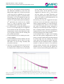
Application Note 4 – v1.0.6 – June 2014 TCSPC measurements with the InGaAs/InP Single-­‐photon counter TCSPC measurements with the
InGaAs/InP Single-photon counter
A typical setup in which the InGaAs/InP Single-­‐
Photon Detection Module is widely employed is a photon-­‐timing one, as illustrated in Figure 1. This setup can be adopted for measurements of fast waveforms of repetitive optical pulses. The implemented technique is commonly known as Time Correlated Single Photon Timing (TCSPC) and is extensively described in Ref. [1] and [2]. As shown in Figure 1, a typical setup consists of a pulsed laser used for exciting a fluorescent sample that reemits photons with an exponential decay. A TCSPC system precisely reconstructs this decay by accurately measuring photon arrival times with respect to a synchronization signal, usually generated (like in this case) by the laser. Before reading this application note it is strongly recommended to read the InGaAs/InP Single-­‐
Photon Detection Module user manual or to have a good background knowledge on how gated-­‐
mode single photon counters work. Measuring nanoseconds decays When using MPD infrared single-­‐photon counters in a TCSPC system, the easiest experimental set-­‐
up is the one used for measuring nanosecond time decays. In this case the most straightforward technique consists in triggering the module with the same frequency of the laser repetition rate, in synchronising the gate window with the fluorescence decay and in setting a gate-­‐
on width slightly longer than the fluorescence curve. In this way the gated mode photon counter behaves as if it would be a free-­‐running module: the detector is always ON when the fluorescence photons arrive. In order to ensure that the photons emitted by the sample impinge on the detector when the gate has been enabled, it is necessary to take particular care to signal propagation delays inside cables, optic fibres and instruments, included the InGaAs/InP module. This information is easily obtained by reading the instruments respective user manuals. For the sake of discussion let’s suppose to use the MPD module for measuring the Instrument Response Function (IRF) of an infrared semiconductor laser driven by the PicoQuant laser driver PDL-­‐800-­‐B [3]. In this case the experimental set-­‐up has no sample under test and the laser pulse is shined, after attenuation, Figure 1: Time Correlated Single Photon Counting set-­‐up using MPD InGaAs/InP single photon counter. AN4 -­‐ 1 Application Note 4 – v1.0.6 – June 2014 TCSPC measurements with the InGaAs/InP Single-­‐photon counter directly onto the detector. Considering the laser driver, the time from the falling edge of the trigger-­‐out signal to the optical pulse out is typically 12 ns (laser internally triggered), while the time from the trigger-­‐in to the optical pulse out is typically 35ns (laser externally triggered). Considering instead the MPD InGaAs/InP photon counter and supposing to set the gate-­‐on window to 20 ns, the time from the trigger-­‐in valid edge to the opening of the gate is 52.7 ns (external triggering of the module) while the time from the trigger-­‐out rising edge to the gate opening is 40.9 ns (internal triggering of the module). When the InGaAs/InP module is configured to use the external trigger, it is impossible to measure the laser pulse unless a very long optic fibre is attached to the laser output as shown in Figure 2. In this example, the laser is set in the internal trigger mode, the reference signal is the laser trigger out pulse and a cable connects the laser trigger output to the photon-­‐counter trigger input. As a consequence the optical pulse is shined after 12 ns from the falling edge of this signal while the gate is opened, with reference to the same edge, after 52.7 ns plus the delay introduced by the cable (10 ns in the example of Figure 2). It means that about 12 m of fibre optic are necessary in order to have the laser pulse inside the gate window (see Figure 2). Instead, by setting the InGaAs module to use the internal trigger and by employing its trigger out signal to synchronise the laser, it is possible to open the gate window exactly when the optical pulse is shined as shown in Figure 3. Let’s suppose, for example, to set the InGaAs/InP module in the internal trigger mode with a 10 MHz reference clock and to connect the trigger out of the control unit to the trigger in of the laser driver input with a coaxial cable 2 m long. In this way, with reference to the signal at the MPD module trigger out, the laser pulse is emitted after 35 ns (laser driver internal propagation delay) + 10 ns (2 m cable for the connection) + 10 ns of fibre optic propagation delay (supposing a 2 m optic fibre connected to the laser head), while the gate window is opened after 40.9 ns with a 20 ns width (see Figure 3). Please also note the 50% duty of the module reference out and that, in this example, a pulse inverter has also been used in order to properly connect the MPD module with the laser driver. This has been necessary since the former is synchronised on the TRIGGER OUT signal rising edge while the latter on its falling edge. In case a user has a longer optical path or optic fibre, then he can simply widen the gate window or decrease the 2m copper cable connection as required. Coming back to the goal of measuring a nanosecond decay pulse, the MPD module configuration is thus started by setting the Figure 2: Timing diagram of various signal when using the InGaA/InP module in the external trigger mode and the reference clock is provided by the employed laser. AN4 -­‐ 2 Application Note 4 – v1.0.6 – June 2014 TCSPC measurements with the InGaAs/InP Single-­‐photon counter Figure 3: Timing diagram of various signal when measuring ns decays with the InGaAs/InP module set in internal trigger mode and used to trigger the employed laser. The reference signal is thus provided by the photon counter. InGaAs/InP module in the “internal trigger mode” and connecting its trigger-­‐out to the trigger-­‐in of the laser. In this way the laser is triggered by the InGaAs module. The laser trigger-­‐out signal is instead used as START of the TCSPC system. The STOP signal to the TCSPC system is given by the photon out of the InGaAs/InP module. In general, when different instruments are connected together, it is very important to verify on which signal edge they synchronise themselves and which are the voltage levels and polarity of all the involved signals in order to attenuate/invert them if necessary for complying with the inputs absolute maximum ratings. For example, in the case shown in Figure 3 it was necessary to invert the trigger output signal of the control unit. In case of using a passive transformer to invert a pulse, we also strongly suggest to terminate first the transmission line and then to attach the transformer. In case of using the PicoHarp 300 [4] as the TCSPC system, the laser sync is usually connected the Channel 0 input and the photon out is normally connected to the Channel 1 input. Instead, if the B&H SPC-­‐130 [5] or similar cards are employed, please read carefully their manual because these cards work in the so called “reverse mode”. The TCSPC technique is normally adopted in order to correctly reconstruct the shape of the temporal response of fast pulses or fast decaying fluorescence pulses (like in our example) by accurately measuring the photon arrival times and not by simply counting the number of detections in a period of time. In order to do this, it must be guaranteed that only a single photon reaches the detector for every single gate. This is a well known requirement which is explained extensively in scientific literature, such as in Ref. [1] and [2]. When this condition is not guaranteed, the so called pile-­‐up effect [1] occurs. In order to avoid the latter, the detection rate must be lower than 5 % (or better, 1 %) of the laser trigger frequency. Detection rate calculation with gated mode detectors is normally not straightforward due to the gated mode regime and the long hold off time normally employed. Anyway, in this case the module duty cycle D is not considered since the Gate window is synchronized with the laser optical pulse and thus all the laser photons reach always the detector when the detector is on: the SPAD behaves as if it would be operated in free running mode. Only the correction for the hold-­‐
off time must be implemented. In addition, the effect of the DCR and of the afterpulsing is considered negligible: the minor error that is eventually committed is conservative. As a consequence, the light source must be properly attenuated in order to satisfy only the following condition: 𝑇!"
𝐶𝑅 < 5% ∙ 𝑓!"#$% − 𝐶𝑅 ∙
𝑇!"#$%
AN4 -­‐ 3 Application Note 4 – v1.0.6 – June 2014 TCSPC measurements with the InGaAs/InP Single-­‐photon counter i.e. the light source must be properly attenuated so that module count rate is smaller than 5 % (or 1 %) of the valid laser frequency, which is the frequency that one obtains once considering only the laser pulses that were shined when the module was in the ON state. CR is the module count rate as measured at a counter, THO is the hold-­‐off time, 𝑇!"#$% = 1 𝑓
, and flaser is the !"#$%
laser repetition rate. By simplifying the previous equation, one obtains: 𝐶𝑅
< 5% ∙ 𝑓!"#$% 1 − 𝐶𝑅 ∙ 𝑇!"
Measuring microseconds decays When the fluorescence lifetime to be measured is longer, in the order of microseconds, the recommended settings for using at best the MPD InGaAs/InP single-­‐photon counter are different than the previous case. Such fluorescence decays is typical for example of some infrared quantum dots. In this case, laser repetition rates are in the order of tens or few hundreds of kHz at maximum, in order to avoid aliasing effects with the decays. With such Figure 4: Measure of a ~2µs decay with a gated mode photon counter and a moving gate window. fluorescent sources, setting up a TCSPC might not be easy and the condition on detection rate, for avoiding the pile-­‐up effect, could impair the measurement acquisition time. The first measurement technique one could imagine is shown in Figure 4: the use, as in the previous case, of the same repetition frequency both for the laser and the module; the synchronization of both the laser and the photon counter triggering references; the use of the longest gate-­‐on width of the InGaAs module. Unfortunately, since this window is at most only 500 ns long while the decay lasts for few µs, it would be necessary to acquire different TCSPC measurements, each one obtained by progressively increasing the time shift between the laser and the gate window, in steps of 500ns (same of the gate-­‐on window). This method allows to acquire different “slices” of the decay curve and use the TCSPC software to sum all of them together as shown in Figure 4. Drawbacks of this technique are a longer acquisition time and the necessity of an additional instrument that is able to generate precision delays in the order of microseconds. In order to avoid both issues, the suggested experimental set-­‐up is the following: -­‐ the photon counter is set at a frequency at least 100 times faster than the laser repetition rate; -­‐ laser and photon counter are synchronised; -­‐ gate window is kept in the nanosecond range. For the sake of clarity, let’s suppose to measure an infrared decay with a lifetime of 2 µs. In this case the recommended test set-­‐up would be: ü set the InGaAs/InP module in the internal trigger mode with a repetition rate of 10MHz (period 100 ns). ü by using a frequency divider, use the TRIGGER OUT of the module for triggering the laser at a repetition frequency of 100 kHz (10 μs period) synced with the module. For this purpose the MPD picosecond delayer (2nd generation [6]) could be used. Another possibility would be AN4 -­‐ 4 Application Note 4 – v1.0.6 – June 2014 TCSPC measurements with the InGaAs/InP Single-­‐photon counter ü
ü
ü
ü
the use of a two outputs function generator like Tektronix’s AFG3102 [7]. Also, since the MPD module trigger out is a square wave with a 50% duty and an amplitude of 3.3V, some signal conditioning might be required before connecting it to a laser TRIGGER IN input (as already explained). Please refer to laser user manuals. If using the MPD picosecond delayer (2nd generation) this would not be needed since it is able to generate correct pulses starting from square wave input signals. As a starting point, set the gate window (TON) to 20 ns or less depending on the brightness of the sample and the actual photon counter afterpulsing. TON will be then adjusted in order to set a proper counting rate for avoiding the pile-­‐up effect (see later). set the hold-­‐off to 10 μs for keeping the after-­‐
pulsing negligible. set the multichannel analyser (MCA), with the highest possible bin but of course no more than 100 ns. In case of using a PicoHarp 300 [4] set bins of 512 ps. Use the TON to adjust the count rate up to 5 % (1 %) of the laser frequency, i.e. 5 kc/s (1 kHz), as measured by a counter with no correction for the module duty cycle or hold-­‐off time. If the laser power can be adjusted, it is also suggested to decrease the TON and increase the laser power: the TCSPC acquisition will have a better dynamic range (this the positive effect of the gate in timing applications) and shorter acquisition time. Summarizing, by using the suggested technique the decay curve to be measured is acquired only during “sampling windows”, TON time long (20 ns in our example), every 100 ns or less (i.e. about two orders of magnitude smaller compared to the decay to be measured) as shown in Figure 5. Each “sampling window” would be composed by acquisition bins of 512 ps (or more depending on the actual settings of the TCSPC system). In the example shown in Figure 5 the sampling effect has been greatly exaggerated for sake of clarity; in real life measurements the decay would be much longer and the sampling rate would result much more fine and less coarse. With this technique the time needed to obtain a complete measure is exactly the same as if an ideal free running module would be used. The difference between the free running and the gated one relies in the fact that with the gated mode only a Figure 5: Example of measurement of a 500ns single exponential decay with a TCSPC system using an ideal free running module (violet) and a gated mode MPD InGaAs/InP single photon counter with the described “sampling” technique (green). AN4 -­‐ 5 Application Note 4 – v1.0.6 – June 2014 TCSPC measurements with the InGaAs/InP Single-­‐photon counter sampled curve and not the full one is acquired. Finally, if it is not possible set the TCSPC bins with a 100 ns width, in order to simplify the acquired decay analysis, it is also possible, after the end of the acquisition, to bin together all the bins in a “sampling window” thus obtaining a real sampling of the decay curve at a sampling rate equal to the InGaAs module internal clock. With the suggested technique, the module counting rate has been used for avoiding the pile-­‐
up effect with no correction for duty cycle or hold-­‐off time. The reason lies in the fact that for every fluorescence (laser) pulse, the gate window is opened many times, each with the same chance of detecting it and the fact that when the detector is triggered only the next laser pulse is missed at most (because the hold-­‐off time in this case is always kept equal or shorter than laser frequency). Anyway, by keeping the counting rate low (only a percentage of the actual laser repetition rate), even the skipped pulses are low. It means, thus, that for each laser pulse the module is enabled only during the sampling times but it is able to measure only the first photon-­‐
per-­‐pulse that triggers it (similarly to a free running module): for avoiding the pile-­‐up effect only the counts measured during the ON time (i.e. what has been actually measured with a counter) must be lower than 5 % (1 %) of the laser frequency. Also any distortion due to the long hold-­‐off is kept negligible because of the low count rate with respect to the laser frequency. Measuring millisecond decays Finally let’s consider the case where emitters with milliseconds lifetime should be measured. For example, let’s suppose to have fluorescent emitters at around 1.3-­‐1.5 µm with an excited state lifetime of about 3.5 ms. Since lifetimes are so long, the excitation laser repetition rate can not be too high. For example the laser repetition rate in this case should be around 50 Hz or 25 Hz (20 ms or 40 ms period respectively). Due to this very low frequency, a smart technique that is able to collect as many photons as possible while still avoiding the pile up effect must be devised: a “standard” TCSCP experiment, with the laser at 50 Hz, should collect at maximum 2.5 photons per second, in order to avoid the pile-­‐up, and the measurement would last many hours. For this reason, in order to obtain accurate results without incurring in such long measurement times, we propose the following technique: ü set the InGaAs/InP module repetition rate to 100 kHz. In this way the period would be 10 μs. ü Set the laser to 50 Hz, synchronized with the InGaAs modules like in previous example. ü set the hold-­‐off to a value small enough so that no gates are skipped whenever an hold-­‐
off is applied. In this way the hold-­‐off is the gate-­‐off period. For example, if using a 100 kHz repetition rate and a gate window of 50 ns, set the hold-­‐off to a value smaller than 9.95 µs. ü set your multichannel analyser in "multi-­‐
stop" configuration, i.e. for each laser trigger it will record the arrival times of all the photons that arrive between one laser sync and the next one and not only the first one. (with a PicoHarp 300, T3 mode should be selected) ü the decay curve is now sampled like in the previous paragraph but with a sampling period of 10 µs ü download the data in your computer, bin the arrival times so that the bin matches InGaAS/InP module period (10 μs in our example) and visualise the sampled decay. ü in order to avoid the pile-­‐up effect, the condition to respect now is that every single sampling bin has to count less than 5% (1%) of the laser repetition frequency. If, for AN4 -­‐ 6 Application Note 4 – v1.0.6 – June 2014 TCSPC measurements with the InGaAs/InP Single-­‐photon counter example, a laser repetition rate of 50 Hz is selected, then the requirement is to count less than 2.5 photons per second and per bin. Of course, if the "highest bin" satisfies this condition, then also all the other bins will satisfy it. This happens since the module is enabled during the sampling times (gated mode detector) only and no sampling time is ever missed due the hold-­‐off, which is now smaller than the sampling period. The pile-­‐
up effect happens when the absorption of a photon causes the detector to be blind in detecting the other photons of the same laser pulse. Since now no pulses are skipped, the only requirement is to have a small probability to have two or more photons in each sampling bin. This requirement is easily obtained by adjusting the gate-­‐on width and setting it depending on the detector noise and on the sample brightness. Remember also that the 5 % applies only on the signal. With such technique, it is then possible to get a module counting rate in the order of tens of kc/s (and not 2.5 c/s as initially thought) and still respecting the TCSPC requirement. Finally it is worth stressing that this measurement technique works thanks to the trick with the hold-­‐off, that allows to have a long off-­‐time after every avalanche and at the same time to avoid any gate-­‐on window skipping due to a previously occurring avalanche. Equivalent free-­‐running mode Independently on the length of the decay time constant, the MPD module can be set in a particular configuration, called “equivalent” free running mode, that allows to acquire the decay curve as if the module would be working in free running. This configuration is achieved simply by setting the module in the internal trigger mode, and leaving it uncorrelated with the laser frequency: no correlation should exist between the laser pulse and the internal trigger. In this case the gate-­‐on window is moving in time and only when it is, by chance, synchronised with the laser it measures the laser pulse; when it is not, it measures only noise. Basically it is as if, for every laser trigger, the gate-­‐on window is randomly opened in the TCSPC observation window with a uniform probability. The module behaves thus like free-­‐running module and not a gated one, but, not being synchronised with the laser means also that photons are lost when the gate-­‐on window is not aligned with the laser pulse: the equivalent free running mode has been achieved at the expense of module detection efficiency which is now reduced by a factor equal to the current duty cycle. Another drawback of this operating mode is that the actual dark counting rate remains the same, compared to the situation where the MPD module is biased exactly in this same conditions and it is also synchronised with the laser pulses, but the S/N is worse because of the reduced detection efficiency. A worse S/N ratio in a TCSPC measurement means a worse dynamic range in the acquired histogram. The best settings to employ equivalent free running mode are a MPD module frequency of 2 MHz (500 ns of period) and TON as long as possible without increasing the noise too much. In this condition, the maximum TON is 450 ns thus limiting the maximum duty cycle to 90 %. Note that when a module works in equivalent free running mode, the gate-­‐on window disappears in the TCSPC histogram. AN4 -­‐ 7 Application Note 4 – v1.0.6 – June 2014 TCSPC measurements with the InGaAs/InP Single-­‐photon counter References 1.
Lakowicz, J. R., Priciples of Fluorescence Spectroscopy, 3rd Edition, Springer, New York, 2006. 2.
O’ Connor, D.V.O., Phillips, D., Time-­‐correlated Single Photon Counting, Academic Press, London, 1984. 3.
PDL-­‐800-­‐B, picosecond pulsed diode laser driver, User manual (www.Picoquant.com). 4.
PicoHarp 300, standalone TCSPC module, User manual (www.Picoquant.com). 5.
SPC-­‐130, TCSPC card, User manual (www.becker-­‐hickl.de). 6.
Picosecond Delayer, devices.com) 7.
AFG3000 series (www.tek.com). datasheet (www.micro-­‐photon-­‐
Copyright and disclaimer No part of this manual, including the products and software described in it, may be reproduced, transmitted, transcribed, stored in a retrieval system, or translated into any language in any form or by any means, except for the documentation kept by the purchaser for backup purposes, without the express written permission of Micro Photon Devices S.r.l. All trademarks mentioned herein are property of their respective companies. Micro Photon Devices S.r.l. reserves the right to modify or change the design and the specifications the products described in this document without notice. Contact For further assistance and information please write to support@micro-­‐photon-­‐devices.com AN4 -­‐ 8