Download RUMD tutorial

RUMD Tutorial
RUMD Development Team
March 16, 2015
Contents
1 Introduction
1.1 Features . . . . . . . . . . .
1.2 User philosophy . . . . . . .
1.3 Installation . . . . . . . . .
1.4 Setting the path for python
.
.
.
.
.
.
.
.
.
.
.
.
.
.
.
.
.
.
.
.
.
.
.
.
.
.
.
.
.
.
.
.
.
.
.
.
.
.
.
.
.
.
.
.
.
.
.
.
.
.
.
.
.
.
.
.
2
2
2
3
4
2 Level 1: How to run your first simulation with RUMD
2.1 The initial condition . . . . . . . . . . . . . . . . . . . . .
2.2 Executing your first program using the python interface .
2.3 Setting options with the python interface . . . . . . . . .
2.3.1 Choosing the potential and its parameters . . . . .
2.3.2 Choosing the integrator . . . . . . . . . . . . . . .
2.3.3 Controlling how frequently to write output . . . .
2.4 Post processing . . . . . . . . . . . . . . . . . . . . . . . .
2.5 Simulating molecules . . . . . . . . . . . . . . . . . . . . .
.
.
.
.
.
.
.
.
.
.
.
.
.
.
.
.
.
.
.
.
.
.
.
.
.
.
.
.
.
.
.
.
.
.
.
.
.
.
.
.
.
.
.
.
.
.
.
.
.
.
.
.
.
.
.
.
.
.
.
.
.
.
.
.
.
.
.
.
.
.
.
.
.
.
.
.
.
.
.
.
.
.
.
.
.
.
.
.
.
.
.
.
.
.
.
.
.
.
.
.
.
.
.
.
5
5
5
7
8
8
8
9
12
3 Level 2: Fine control
3.1 Controlling how the simulation run is divided into blocks . . . . . . . . . . . . .
3.2 Controlling what gets written to energies and trajectory files . . . . . . . . . . .
3.3 Changing the sample volume within the script . . . . . . . . . . . . . . . . . . . .
3.4 Options for Run: Restarting a simulation, suppressing output, continuing output
3.5 Getting optimum performance via the autotuner . . . . . . . . . . . . . . . . . .
14
14
14
15
15
16
4 Level 3: How to implement your own pair potential in RUMD
17
.
.
.
.
.
.
.
.
.
.
.
.
.
.
.
.
.
.
.
.
.
.
.
.
1
.
.
.
.
.
.
.
.
.
.
.
.
.
.
.
.
.
.
.
.
.
.
.
.
.
.
.
.
.
.
.
.
.
.
.
.
.
.
.
.
2
1
Introduction
The CUDA project has enabled scientists to utilise NVIDIA’s many-core Graphical Processor
Unit (GPU) to solve complex computational problems. Beside being a very fast processor the
GPU is relatively cheap, and is thus an ideal computational unit for low-cost high performance
supercomputing. Scientific software is currently being developed in a very rapid pace by many
different groups world wide, and today there exists optimized software for fluid dynamics and
matrix operations just to name a few.
RUMD [‘rOm di• ] is a high-performance molecular dynamics simulation software package
optimized for NVIDIA’s graphics cards. RUMD is designed for small to medium size systems of
spherical particles and simple molecules. RUMD is developed at The Danish National Research
Foundation’s centre “Glass and Time” which is located at the Department of Sciences, Roskilde
University.
1.1
Features
RUMD currently supports:
• van der Waals type pair potentials: Lennard-Jones, Gaussian core, Inverse Power Law, and
more. It is easy to implement new pair potentials.
• Bond stretching potentials: Harmonic and FENE
• Multicomponent simulations
• NVE and NVT ensemble simulations
• python interface
• Post simulation analysis tools
In the very near future we plan to support:
• Bond constraint dynamics
• Angle bending potentials
• Diheadral potentials.
• Additional ensembles
• Couloumb interaction potentials
1.2
User philosophy
We have defined five users of RUMD:
1. A user at level 1 is one who can write or copy a simple python script (for example the one
given later in this tutorial) to run a standard molecular dynamics simulation, and use the
provided analysis tools to perform standard analysis of the output. This user can make
some basic choices, such as the potential, the integrator, and controlling the frequency of
output.
3
2. This user understands the deeper structure of the code—that is the different kinds of
classes/objects, the relations between them, and their interfaces—and understands how
the python language works, and can therefore write more sophisticated python scripts
which access the full power and flexibility of RUMD.
3. A user at level 3 is one with minimal experience in C++ can write her own (pair-)potential
functions, to be available as classes derived from PairPotential.
4. This user can write their own analysis programs in C++, but does not need to know
anything about GPU programming, since analysis is generally carried out on the CPU.
5. RUMD developer. Must have a good knowledge of C++, CUDA programming and knowledge of Subversion.
This tutorial will bring you from level 1 to level 3. Note that level 3 is higher than level 2 in
that it requires the user to write some C++ code and re-compile the code, but that involves
a relatively limited list of things to do. Level 2, which stays at the python level, but involves
access to almost all of the underlying C++ functionality, could take longer to master.
1.3
Installation
For Debian-like systems, RUMD can be installed as a package. Use the following repository
entries appended to /etc/apt/sources.list or in a file in /etc/apt/sources.d/
deb http://debian.ruc.dk/rumd squeeze main
deb-src http://debian.ruc.dk/rumd squeeze main
To install RUMD simply use an equivalent of:
apt-get install rumd
You need to have root privileges, of course.
You can also build the package from the source. To do so, download the source code from
the RUMD homepage
www.rumd.org/download.html
and unpack the file using
tar xzvf rumd-X.X.X.tar.gz
where X.X.X is the version number. Enter the source directory
cd rumd-X.X.X
and build the package by typing
make
To test your installation use
make test
This test will take approximately 5-10 minutes.
Notice, you cannot type make install since the default path is different from system to
system. We will refer to the installation path as <RUMD-HOME>
4
1.4
Setting the path for python
In a proper installation the python modules should be located in a standard place where python
will automatically find them. This may not be possible if you do not have root privileges,
however. If you have compiled the software yourself, you need to set the environment variable
PYTHONPATH as follows (this is for C-shell, so it would go in your .cshrc file; for other shells
there is a corresponding command)
setenv PYTHONPATH <RUMD-HOME>/Swig:<RUMD-HOME>/Python:<RUMD-HOME>/Tools
5
2
Level 1: How to run your first simulation with RUMD
This tutorial assumes basic GNU/Linux knowledge, a successful installation of RUMD and a
little portion of gumption mixed with interest in molecular dynamics. For plotting the results
from simulations it is assumed that xmgrace is installed, but other plotting programs can be
used if you prefer.
The basic work-flow of doing simulations is:
• Specify initial condition, i.e., the initial positions and velocities to be used in the simulation.
This also involves the number of particles (N ) and the (initial) density (ρ ≡ N/V ).
• Running the actual simulation. This can be done interactively or by a script in python.
It includes defining how particles interact with each other (i.e., the potentials used), what
integrator to use (and the associated parameters, e.g., time-step and temperature.)
• Post-processing data analysis.
The following sub-sections will take you through these steps.
2.1
The initial condition
When doing simulations it is often convenient to use the end result of one simulation as the
initial condition to a new simulation. However, sometimes you need to generate a fresh initial
condition. This can be done as described below.
Make a directory where you want your first simulation to be performed. Call it e.g. ~/Test/.
Go to the ~/Test/ directory, run the rumd_init_conf_FCC program (make sure RUMD_home/Tools/
is in your path). This is a GNU Octave program that generates an fcc crystal, which can be used
as an initial condition. It will first ask for the density, the temperature, the number of unit cells
nc in each direction, the total number of particles (up to 4n3c ) and finally it asks for the number
of different particles of each type. The program produces a file called start_fcc.xyz.gz with
the specified information, which can be used as initial condition in an simulation.
Produce an initial configuration with the density and temperature set to 1.0, set the total
number of particles to 1000 and let them all be of type 0.
2.2
Executing your first program using the python interface
In this first example we will simulate a single component Lennard–Jones liquid. We will work
with python interactively, so that you can get a feel for what is possible. For production runs
you will normally make a script containing the appropriate python commands. Start python by
typing “python” and pressing enter. You will get a prompt that looks like “>>>”. Type
from rumd import *
This will import the main RUMD classes into the global namespace1 (these are actually C++
classes, but we can “talk” to them through python). These are enough to write scripts and
thereby run simulations, but to simplify this process, particularly for newcomers, there is an
extra python class called rumdSimulation: type
from rumdSimulation import rumdSimulation
This class combines access to the main data-structures with the main integration loop and various
functions for controlling output etc. To start a simulation we first create a rumdSimulation
object, passing the name of a starting configuration file:
1 Alternatively (recommended by some to avoid possible name clashes in the global namespace) one can type
import rumd, and then all of the class-names, etc., must be prefixed by rumd., for example rumd.IntegratorNVE.
6
sim = rumdSimulation("start.xyz.gz")
Here sim is an arbitrary name we choose for the object. Next we choose an NVT integrator,
giving the time-step and temperature:
itg = IntegratorNVT(timeStep=0.0025, targetTemperature=1.0)
Having an integrator object, we need to connect it to the simulation:
sim.SetIntegrator(itg)
Next we need to choose the potential. For 12-6 Lennard-Jones we create a potential object,
giving it the name pot, as follows:
pot = Pot_LJ_12_6(cutoff_method=ShiftedPotential)
The mandatory argument cutoff_method specifies how the cut-off of the pair-potential is to be
handled. It must be one of ShiftedPotential (the most common method, where the potential
is shifted to zero), ShiftedForce or NoShift We need to set the parameters, which is done using
the method SetParams. The arguments to this method depend on which potential class you are
working with, but they can be found by typing
help(pot.SetParams)
which displays a help page generated from the “docstring” of the method (alternatively type
print pot.SetParams.__doc__). In particular this includes a list of the arguments:
SetParams(self, unsigned int i, unsigned int j, float Sigma,
float Epsilon, float Rcut)
The first one, self, represents the object itself, and is not explicitly given when calling the
function. The next two define which particle types we are specifying parameters for—we just
have one type of particle so both will be zero; the two after that are the standard Lennard-Jones
length and energy parameters, while the last is the cut-off in units of Sigma. Press Q to exit the
help screen. We choose the following:
pot.SetParams(0, 0, 1.0, 1.0, 2.5)
Note that we can also use python’s “keyword arguments” feature to specify the arguments, which
can then be in any order, for example:
pot.SetParams(i=0, j=0, Epsilon=1.0, Rcut= 2.5, Sigma=1.0)
The potential also needs to be connected to the simulation:
sim.SetPotential(pot)
Now we are ready to run a simulation. To run a simulation with 20000 time steps, we just write
sim.Run(20000)
Various messages will be printed to the screen while it is running (these can be turned off with
sim.SetVerbose(False). If we like, we can get the positions after the 20000 steps by getting
them as a numpy array (numpy, or numerical python, is a package that provides efficient arraybased numerical methods), and in particular look at the position of particle 0 by typing
pos = sim.sample.GetPositions()
print pos[0]
However more likely we will run an analysis program on the output files produced by the simulation during the operation of the Run function. The available analysis programs are described
below in subsection 2.4 in their command-line forms. Some of them (eventually all) can also
be called from within python. For now let’s write a configuration file for possible use as a
starting point for future simulations. Here we go a little deeper into the interface. Objects of
type rumdSimulation have an attribute called "sample" of type Sample (the main C++ class
representing the sample we are simulating). We call its WriteConf method as follows:
sim.WriteConf("end.xyz.gz")
7
Type Ctrl-D to exit python. Next we would like to make scripts. Here is the script that contains
the commands we have just worked through (the lines starting with # are comments):
from rumd import *
from rumdSimulation import rumdSimulation
#create simulation object
sim = rumdSimulation("start.xyz.gz")
# create integrator object
itg = IntegratorNVT(timeStep=0.0025, targetTemperature=1.0)
sim.SetIntegrator(itg)
# create potential object
pot = Pot_LJ_12_6(cutoff_method=ShiftedPotential)
pot.SetParams(0, 0, 1.0, 1.0, 2.5)
sim.SetPotential(pot)
sim.Run(20000)
sim.WriteConf("end.xyz.gz")
If this script is saved as a file called, for example, run.py (it must end in .py), then it is run by
typing python run.py. This will exit python when finished. To leave python on after the script
has completed, type python -i run.py (-i means run in interactive mode). If it is to be run on
a batch queue, the appropriate PBS commands should be included in comments at the top as
follows:
#!/usr/bin/env python
# pass PYTHONPATH environment variable to the batch process
#PBS -v PYTHONPATH
#PBS (other PBS commands here)
#PBS
#PBS
# this ensures PBS jobs run in the correct directory
import os, sys
if os.environ.has_key("PBS_O_WORKDIR"):
os.chdir(os.environ["PBS_O_WORKDIR"])
sys.path.append(".")
from rumd import *
(etc)
It should be submitted using qsub run.py. Note that the indentation of the two lines following
the if statement is important!
2.3
Setting options with the python interface
Here we present some of the options available for controlling simulations.
8
2.3.1
Choosing the potential and its parameters
Probably the most important thing a user needs to control is the potential. Different potentials
are represented by different classes; objects are created just as above, so for example:
# generalized LJ potential (here m=18, n=4)
potential = Pot_gLJ_m_n(18,4, cutoff_method=ShiftedPotential)
# inverse power-law (IPL) with exponent n=12
potential = Pot_IPL_12(cutoff_method=ShiftedPotential)
To set parameters for the potential, call its SetParams method as described above. If a binary
system is to be simulated, the parameters should be set separately for each interaction pair as
follows
potential.SetParams(0, 0, 1.00, 1.00, 1.12246)
potential.SetParams(0, 1, 0.80, 1.50, 1.12246)
potential.SetParams(1, 1, 0.88, 0.50, 1.12246)
Note that Newton’s third law is assumed to hold, so setting the parameters for i=0 and j=1
automatically sets those for i=1 and j=0 (we could also have called SetParams with the latter).
An overview of the available potentials is given in the user manual.
2.3.2
Choosing the integrator
Perhaps the next most important choice is what kind of integration algorithm to use. Above
we did a constant-temperature (NVT) algorithm (the actual algorithm is of the Nosé-Hoover
type). For constant energy (NVE) runs we create the integrator as follows, here passing only the
time-step:
itg = IntegratorNVE(timeStep=0.0025)
(Technical note: this creates an object of the same type as IntegratorNVT, but here it defaults to NVE mode—in fact in either case one can switch thermostatting on or off using the
SetThermostatOn() method).
Additional integrators available in RUMD are listed below
Name of Integrator
IntegratorNVE
IntegratorNVT
IntegratorNVU
IntegratorMMC
IntegratorIHS
IntegratorSLLOD
IntegratorMolecularSLLOD
Description
The NVE Leap-frog algorithm.
The Nosé-Hoover NVT algorithm.
Algorithm conserving the total potential energy.
Metropolis NVT Monte Carlo.
Energy minimization via the Leap-frog
algorithm.
Shear an atomic system in the xy-plane
using the SLLOD equations.
Shear a molecular system in the xyplane using the SLLOD equations.
Arguments
timeStep
timeStep, targetTemperature
dispLength, potentialEnergy
dispLength, targetTemperature
timeStep
timeStep, strainRate
timeStep, strainRate
The above integrators are chosen in the usual way with named arguments as given in the table.
2.3.3
Controlling how frequently to write output
To control the output written to files we use the rumdSimulation method SetOutputScheduling.
By default there are two “output managers”: “energies” and “trajectory”. The first is for the
9
files containing potential/kinetic energies and other global quantities, while the second is for
trajectories (configuration files containing the particle positions at different times during the
run). The write-schedule for either manager can be evenly-spaced in time (“linear”), logarithmic
(“logarithmic”), or a kind of combination of the two (“loglin”). Examples of controlling scheduling
include
sim.SetOutputScheduling(
sim.SetOutputScheduling(
sim.SetOutputScheduling(
sim.SetOutputScheduling(
"energies", "linear", interval=50)
"energies", "none" )
"trajectory", "logarithmic" )
"trajectory", "loglin", base=4, maxInterval=64 )
The first causes energies to be output equally spaced (linear) in time, once every 50 time steps,
while the second turns energy writing off. The third will cause logarithmic saving of configurations (where the interval between saves doubles each time within a “block”, starting with 1.
The fourth does logarithmic saving starting with interval 4 until the interval 64 is reached, after
which the interval stays fixed at 64 until the end of the block. The details of log-lin are described
in a separate document. By default energies are linear, written every 256 steps, and trajectories
are logarithmic.
2.4
Post processing
The post processing tools are located in the <RUMD-HOME>/Tools/ directory and each one of them
has a help text. To see the help text use the option -h or --help depending on the tool. The actual output files generated by the program are in a directory called TrajectoryFiles. When you
start a new simulation in the same directory, this will be moved to TrajectoryFiles.rumd_bak
as a precaution against accidental overwriting of data. The analysis programs should be run in the
original directory where the simulation was run (they know they should look in TrajectoryFiles
for the data).
rumd_stats produces mean values, variances and standard deviations for specific quantities. The
rumd_stats stdout for the simulation just performed is shown in table 1.
quantity
ke
pe
p
T
Ps
Etot
W
mean value
1.49802
-5.27922
8.64558
0.999677
-0.00404791
-3.7812
7.64591
variance
0.0015541
0.0029679
0.0529826
0.000692101
0.348731
0.00439295
0.052637
standard deviation
0.0394221
0.0544784
0.23018
0.0263078
0.590535
0.0662794
0.229428
Table 1: rumd_stats output.
Here ke is the kinetic energy, pe is the potential energy, p is the pressure, T is the kinetic temperature, Ps is the Nose Hoover thermostat, Etot is the total kinetic energy and W is the virial. The
program writes the mean and variance in the files energies_mean.dat and energies_var.dat
in one row as the first column of stdout.
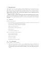
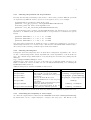
The radial distribution function is computed by typing rumd_rdf -n 1000 -m 1.0 where the
first argument is the number of bins in radial distribution function and the second argument,
10
the minimum time between successive configurations to use, is to avoid wasting time doing
calculations that are very similar (we assume here that the configurations are uncorrelated after
one time unit). Use rumd_rdf -h for a full list of arguments. The output is rdf.dat and for
binary systems the columns are:
r g00 (r) g01 (r) g10 (r) g11 (r). (Single component only has two columns). Plot rdf.dat to
obtain figure 1.
Radial distribution function
4
g(r)
3
2
1
0
0
1
2
r
3
4
5
Figure 1: Radial distribution function.
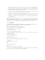
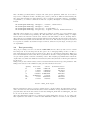
The static structure factor can be obtained when the radial distribution function is computed.
It is done by typing rumd_sq 2 20 1 where the first argument is the start q value, the second
argument is the final q value and the third argument is the density. The stdout is the q value for
the maximum of the first peak and it is written in a file called qmax.dat. The static structure
factor is written in Sq.dat and is structured like rdf.dat. Plot Sq.dat to obtain figure 2.
The mean square displacement and the self part of the incoherent intermediate scattering
Static structure factor
4
S(q)
3
2
1
0
0
5
10
q
15
Figure 2: The static structure factor
20
11
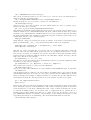
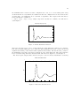
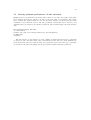
function Fq (t) are calculated with the command rumd_msd. This generates a msd.dat file with
time as the first column and the mean square displacement as a function of time as the second
column (for binary systems there will be two columns), and a file Fs.dat with a similar structure.
Before it can be run however, you must create a file called qvalues.dat which contains one
wavenumber for each time of particle. Typically these correspond to the location of the first peak
in the structure factor, so one could copy the file qmax.dat crated by rumd_sq. rumd_msd also
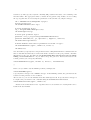
calculates gaussian parameter alpha2.dat. See figure 3 and 4 for mean square displacement and
self part of incoherent scattering function. The post processing analysis tools are summarized
Mean square displacement
2
<r (t)>
1
0,01
0,0001
0,001
0,01
0,1
1
10
100
Time
Figure 3: Mean square displacement.
Self part of intermediate scattering function
qmax = 7.1
0,8
F(qmax,t)
0,6
0,4
0,2
0
0,001
0,01
0,1
1
10
100
Time
Figure 4: Self part of the intermediate scattering function evaluated at the q value of the maximum of the first peak in the structure factor.
in table 2. It is evident from table 2 that rumd_rdf has to be performed before rumd_sq and
12
Tool
Input
rumd_stats
none
rumd_rdf
none
rumd_sq
rdf.dat
rumd_msd
Output
std.out: table 1
energies_mean.dat
energies_var.dat
std.out: Simulation info
rdf.dat
sdf.dat
std.out: qmax(s)
Sq.dat
qmax.dat
std.out: Simulation info
msd.dat
Fs.dat
FsSq.dat
alpha2.dat
qvalues.dat
Arguments
none
1. num. bins
2. time diff.
1. qstart
2. qfinal
3. density
none
Table 2: Post processing tools, their input, output and the arguments.
rumd_sq before rumd_msd. If you only are interested in the mean square displacement and know
which q-values to use it is not necessary to run rumd_rdf and rumd_sq first. Then you just have
to create a file called qvalues.dat with the appropriate q-values before running rumd_msd.
2.5
Simulating molecules
With RUMD you can simulate molecular systems. The intra-molecular force field includes bond,
angle and torsion interactions. The total potential energy due to intra-molecular interactions
excluding possible pair potentials is given by
U (~r) =
5
X X
1 X (i)
1 X (i)
(i)
n
ks (rij − lb )2 +
kθ [cos(θ) − cos(θ(i) )]2 +
c(i)
n cos (φ),
2
2
n=0
bonds
angles
(i)
(1)
dihed
(i)
where ks is the spring force constant for bond type i, kθ the angle force constant for angle
(i)
(i)
(i)
force type i, and cn the torsion coefficients for torsional force type i. lb and θ0 are the zero
force bond length and angle, respectively.
Beside the standard harmonic bond potential RUMD also supports simulation of rigid bonds
using constraint method as well as the Finite Extensible Nonlinear Elastic (FENE) potential
"
2 #
1 2 X
rij
U (~r) = − kR0
,
(2)
ln 1 −
2
R0
bonds
where k = 30 and R0 = 1.5 (in reduced units). At the moment the constraint method is
applicable for molecules with few constraints.
Example
In all one starts by creating (or copying and modifying) a topology file (with extension .top).
Examples can be found in the subdirectory Conf/Mol, in particular one called mol.top, which
is associated with a configuration file ExampleMol.xyz.gz. Copy both of these files to your
13
test directory. They specify a system containing 100 polymeric molecules, each consisting of 10
monomer units. The appropriate lines to include in the python script include one for reading
the topology file and one for setting the parameters of the (in this case) single bond-type.
sim = rumdSimulation("ExampleMol.xyz.gz")
# read topology file
sim.ReadMoleculeData("mol.top")
# create integrator object
itg = IntegratorNVE(timeStep=0.0025)
sim.SetIntegrator(itg)
# create pair potential object
potential = Pot_LJ_12_6(cutoff_method=ShiftedPotential)
potential.SetParams(i=0, j=0, Epsilon=1.0, Sigma=1.0, Rcut=2.5)
sim.SetPotential(potential)
# define harmonic bond and its parameters for bonds of type 0
sim.SetBondHarmonic(type=0, lbond=0.75, ks=200.0)
sim.Run(20000)
Note that when you specify the bond parameters after calling SetPotential contributions from
those bonds will automatically be removed from the calculation of the pair potential, otherwise
this will not be the case. For this reason it is important that you call SetPotential before
calling sim.SetBondHarmonic. If you wish to keep the pair force interactions between the
bonded particles you can specify this using
sim.SetBondHarmonic(type=0, lbond=0.75, ks=200.0, exclude=False)
2
In the case you wish to use the FENE potential you simply use
sim.SetBondFENE(type=0)
to specify that bond type 0 is a FENE bond type. In the FENE potential, the pair interactions
between bonded particles are not excluded.
As noted above, you can also simulate molecules with rigid bonds. To specify that bond type 0
is a rigid bond you add the bond constraint using the SetBondConstraint method
sim.SetBondConstraint(type=0, lbond=0.75)
Details of the format used for the .top files and on tools available for creating them can be
found in the user manual.
14
Table 3: Identifier and column-label for the main quantities that can be written to the energies
file.
identifier
potentialEnergy
kineticEnergy
virial
totalEnergy
temperature
pressure
volume
stress_xx
column label
pe
ke
W
Etot
T
p
V
sxx (a)
(a)
Potential part of atomic stress.
Similarly yy, zz, xy, etc
3
Level 2: Fine control
The user at level 2 can use the full rumdSimulation interface to control many details of the
simulation. Here we present, mostly in the form of python code-snippets, some of the more
advanced aspects of the interface, though without trying to present a complete documentation.
The next step is to look on the RUMD web-page (www.rumd.org) under “example scripts” for
ideas about how to get the most out of RUMD.
3.1
Controlling how the simulation run is divided into blocks
The simulation output is divided into blocks of size blockSize. By default the block-size is
chosen when Run is called, so that there will be of order 100-200 blocks in the given number
of time-steps. Sometimes it is useful to explicitly specify the block-size (this will sometimes be
necessary when using log-lin because there are some constraints on the block-size in relation to the
log-lin parameters). The following will set the blockSize (we denote by sim the rumdSimulation
object):
sim.SetBlockSize(1024)
3.2
Controlling what gets written to energies and trajectory files
To change what gets written we call the SetOutputMetaData method, which functions similar
to SetOutputScheduling in that it takes a string with the name of the output manager, and
one or more keyword arguments specifying either that a parameter should be included or not, or
what the overall precision should be.
sim.SetOutputMetaData("energies",totalEnergy=False,stress_xy=True, precision=7)
which turns off writing the total energy, turns on writing the xy component of the stress tensor,
and sets the precision to seven decimal places. Table 3 shows the most important available
quantities. To each of these are associated two strings: an “identifier” for use in scripts, to refer
to a given quantity when turning it “on” or “off”; and a “column-label”, which appears in the
comment-line of the energies file to identify which column corresponds to which quantity.
15
For simulations in which more than one potential is present, the contributions from different
terms to the total potential energy can be included in the energies file. Each potential class has
an ID string. For example for Pot_LJ_12_6 it is “potLJ”. If desired the ID string can be changed
(for example to the simpler “LJ”) via
pot.SetID_String("LJ")
In the case of contributions to potential energy this ID-string functions as both the identifier in
scripts, and the column-label in the energies-file. So for example, after changing the ID-string to
“LJ” as above, to cause it to be written we would write
sim.SetOutputMetaData("energies", LJ=True)
There is a mechanism for additional quantities to be defined and included in the energies file,
via classes of type ExternalCalculator. This is described in the user manual.
3.3
Changing the sample volume within the script
It can be useful to take a configuration corresponding to one density and rescale the box and
particle coordinates such that it has a different density. This is accomplished by the following
lines (which also show how to get the current volume and number of particles).
nParticles = sim.GetNumberOfParticles()
vol = sim.GetVolume()
currentDensity = nParticles/vol
sim.ScaleSystem( pow(newDensity/currentDensity, -1./3) )
where newDensity is understood to be the desired density.
3.4
Options for Run: Restarting a simulation, suppressing output,
continuing output
Under default conditions a “restart file” will be written, once per output-block. If a simulation is
interrupted (due to hardware problems for example), it can be restarted from the last completed
block (here 12) by
sim.Run(20000, restartBlock=12)
where the original number of time-steps should be specified, and the last completed block can
be found by looking at the file “LastComplete_restart.txt” in TrajectoryFiles. It is possible to
suppress writing of restart files (so restarts will not be possible), and all other output, by calling
sim.Run(20000, suppressAllOutput=True)
This might be done for example, during an initial period of equilibration, although if this is
planned to take a long time, it may be advisable to allow restart files to be written, in case of
possible interruptions.
To avoid re-initializing the output, so that repeated calls to Run will append to the existing
energies and trajectory files, do
sim.Run(20000, initializeOutput=False)
This will give an error if Run was not called previously in the normal way (initializeOutput=True,
which is its default value).
16
3.5
Getting optimum performance via the autotuner
RUMD involves several internal parameters whose values do not affect the results of the simulation within round-off error, but they can have a noticeable effect on performance. The easiest
way to identify the optimal values is to use the autotuner, which is a python script that takes
a simulation object which is ready to run (the potential(s) and integrator have been set), and
determines the best values for the internal parameters. The following snippet shows how this is
done.
from Autotune import Autotune
at = Autotune()
[create sim with associated potential(s) and integrator]
at.Tune(sim)
sim.Run()
The time taken to do the tuning is of order a minute for small systems (longer if constraints
are involved). The autotuner writes a file, autotune.dat in the directory. If the simulation is
re-run in the same directory with the same user parameters and on the same type of graphics
card, then the autotuner will simply use the previously determined internal parameters.
17
4
Level 3: How to implement your own pair potential in
RUMD
This tutorial will describe how to implement a new pair potential and test it. Let us say we want
to implement a Gaussian core potential:
r 2
v(r) = ǫ exp −
(3)
σ
When implementing a new pair potential there are a number of things to do:
1. Implement the potential and force into the RUMD source code
2. Include the new potential in the Python interface
3. Compile
4. Test the potential
5. Use it
The PairPotential.h in the directory <RUMD-HOME>/include /rumd contains all the
pair potentials, implemented as classes in C++.
We start with a review of the general 12-6 Lennard-Jones potential - it is the first pair
potential in the file (search for Pot_IPL_12_6). Note that this is not the one most typically
used in simulations; that would be one of its derived classes Pot_LJ_12_6. The difference is only
in how the parameters are specified: for the Pot_IPL_12_6 potential, rather than Epsilon and
Sigma, we specify the coefficients of the IPL terms, A12 and A6. We will make a copy of it and
change it to the Gaussian core potential.
The implementation is split into two major parts: The first part is the function SetParams(...)
which is called by the user via the python interface. The last part is the function ComputeInteraction
where the actual computation (on the GPU) is taking place.
SetParams(...) is called via the python interface once for each type of interaction, with i
and j denoting the types of the two particles involved in the particular interaction. The user
specifies the coefficients A12 and A6 and the cut-off Rcut (in other potentials the parameters might
include a characteristic length σ and characteristic energy ǫ and possibly more parameters). The
parameters of the potential are communicated by storing them in h_params[i][j][]. NOTE:
the correctness of the program relies on h_params[i][j][0] containing the cut-off in absolute
units. In other words, interactions between particles of type i and j are only computed if the
distance between the two particles is less than h_params[i][j][0]. The rest of the stored
parameters are chosen to facilitate fast computation.
The actual computation of the potential and the associated force is done on the GPU by
the function ComputeInteraction(...). When this is called dist2 contains the square of the
distance between the two particles in question, and param contains the appropriate parameters
as set up by SetParams(...). From this information, the function calculates s (i.e. the force,
see below in equation (5)) and the potential. In the Lennard-Jones potential it is convenient to
define two inverse lengths invDist2 and invDist6 to minimize the number of calculations. With
these lengths it is easy to calculate s and the potential energy. (*my_f).w += is the contribution
to the potential energy.
We will now proceed to implement a Gaussian core potential. First step is to write up the
equations we will implement. We will here implement the Gaussian core potential (repeated
18
below)
r 2
v(r) = ǫ exp −
σ
We have to provide the function s which is used by RUMD to calculate the force:
2ǫ
r 2
1 dU (r)
= 2 exp −
s(r) ≡ −
r dr
σ
σ
(4)
(5)
Now copy the entire Lennard-Jones potential and paste it somewhere in the file PairPotential.h.
Replace Pot_IPL_12_6 with Pot_Gaussian (four places). Choose a default identity string, e.g.
SetID_String("potGauss");.
We will change the arguments in the SetParams(...) to match those of the other LJ
potential Pot_LJ_12_6 which uses ǫ and σ instead of A12 and A6 , since the Gaussian potential also
has a characteristic length σ and a characteristic energy ǫ. But we need to make corresponding
changes to the h_params[i][j][]’s. For the Gaussian potential they become:
• h_params[i][j][0] = Rcut * Sigma;
• h_params[i][j][1] = 1.f / ( Sigma * Sigma );
• h_params[i][j][2] = Epsilon;
Note that here the user parameter Rcut is to be interpreted as a scaled cutoff, in units of the
corresponding σ. Now we can write the part taking place on the GPU. Since we do not need any
inverse distances delete the lines computing invDist2 and invDist6. We define instead a float
called Dist2:
float Dist2 = dist2 * param[1];
which is (r/σ)2 . To avoid computing the exponential more than once, we define:
float exponential =
exp(-Dist2);
With these definitions, s is simply implemented as:
float s = 2.f * param[1] * param[2] * exponential;
The next line is the potential:
(*my_f).w += param[2] * exponential;
This finishes the actual implementation, and we now proceed with a number of more technical
changes ensuring that RUMD knows your new pair potential.
• In the file Potentials.i in the directory <RUMD-HOME>/Swig copy the two entries
relating to Pot_IPL_12_6, rename them, and change the arguments to SetParams in accordance with how it was defined in PairPotential.h.
• In the directory <RUMD-HOME> do
make
19
Gaussian core potential
1
Close up at Rcut
0,01
0,8
U(r)/ε
0,005
U(r)/ε
0,6
0
-0,005
2,2
0,4
2,4
2,8
2,6
r
0,2
0
0
1
r
2
3
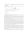
Figure 5: The Gaussian core potential.
If everything compiled without errors the new pair potential will now be available from the
python interface, and you need to test it. Run a simulation as described in the Level 1 tutorial,
but choose the new potential.
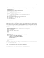
Check that the simulation ran with the correct potential by plotting it by adding
potential.WritePotentials(sim.sample.GetSimulationBox()) to your script. This command produces a file ”potentials_PotID.dat” where the potential v(r) is followed by the radial
force f (r) in each column for all possible particle pairs.
Make sure that the cut-off is done correctly by the program by zooming in on that distance.
An example is shown in figure 5. Next, run a NVE simulation and test that the total energy is
conserved (i.e., have fluctuations that are much smaller than for the potential and kinetic energy).
Have fun with RUMD!