Download RUMD User Manual [Version 3.0]

RUMD User Manual [Version 3.0]
The RUMD development team: Thomas B. Schrøder, Nicholas P. Bailey,
Trond Ingebrigtsen, Jesper Schmidt Larsen, Claire Lemarchand,
Lasse Bøhling, Heine Larsen
c March 2015
Contents
1 Preliminaries and general information
1.1 Availability and latest version . . . . . . .
1.2 RUMD paths and modules . . . . . . . . .
1.3 Basic RUMD scripts . . . . . . . . . . . .
1.4 Acquiring start-configurations . . . . . . .
1.5 Precision for floating-point arithmetic . .
1.6 Maximum system sizes . . . . . . . . . . .
1.7 On the use of the word “block” in RUMD
1.8 How to cite RUMD . . . . . . . . . . . . .
.
.
.
.
.
.
.
.
.
.
.
.
.
.
.
.
.
.
.
.
.
.
.
.
.
.
.
.
.
.
.
.
.
.
.
.
.
.
.
.
.
.
.
.
.
.
.
.
.
.
.
.
.
.
.
.
.
.
.
.
.
.
.
.
.
.
.
.
.
.
.
.
.
.
.
.
.
.
.
.
.
.
.
.
.
.
.
.
.
.
.
.
.
.
.
.
.
.
.
.
.
.
.
.
.
.
.
.
.
.
.
.
.
.
.
.
.
.
.
.
.
.
.
.
.
.
.
.
.
.
.
.
.
.
.
.
.
.
.
.
.
.
.
.
.
.
.
.
.
.
.
.
.
.
.
.
.
.
.
.
.
.
.
.
.
.
.
.
.
.
.
.
.
.
.
.
.
.
.
.
.
.
.
.
.
.
.
.
.
.
.
.
.
.
.
.
.
.
.
.
.
.
.
.
.
.
.
.
2
2
3
3
3
4
4
4
4
2 Pair potentials
2.1 Number of types . . . . . . . . . . . . . . . . . . . .
2.2 Cut-offs . . . . . . . . . . . . . . . . . . . . . . . . .
2.3 Attaching potential objects to the simulation object
2.4 General methods for pair potentials . . . . . . . . . .
.
.
.
.
.
.
.
.
.
.
.
.
.
.
.
.
.
.
.
.
.
.
.
.
.
.
.
.
.
.
.
.
.
.
.
.
.
.
.
.
.
.
.
.
.
.
.
.
.
.
.
.
.
.
.
.
.
.
.
.
.
.
.
.
.
.
.
.
.
.
.
.
.
.
.
.
.
.
.
.
.
.
.
.
.
.
.
.
.
.
.
.
.
.
.
.
.
.
.
.
4
4
6
6
6
3 Other potentials
3.1 TetheredGroup . . . . . . . . . . . . . . . . . . . . . . . . . . . . . . . . . . . . . . . . . . . . . .
7
7
4 Integrators
4.1 IntegratorNVE, IntegratorNVT
4.2 IntegratorNVU . . . . . . . . .
4.3 IntegratorSLLOD . . . . . . . .
4.4 IntegratorMolecularSLLOD . .
4.5 IntegratorIHS . . . . . . . . . .
4.6 IntegratorMMC . . . . . . . . .
.
.
.
.
.
.
.
.
.
.
.
.
.
.
.
.
.
.
.
.
.
.
.
.
.
.
.
.
.
.
.
.
.
.
.
.
.
.
.
.
.
.
.
.
.
.
.
.
.
.
.
.
.
.
.
.
.
.
.
.
.
.
.
.
.
.
.
.
.
.
.
.
.
.
.
.
.
.
.
.
.
.
.
.
.
.
.
.
.
.
.
.
.
.
.
.
.
.
.
.
.
.
.
.
.
.
.
.
.
.
.
.
.
.
.
.
.
.
.
.
.
.
.
.
.
.
.
.
.
.
.
.
.
.
.
.
.
.
.
.
.
.
.
.
.
.
.
.
.
.
.
.
.
.
.
.
.
.
.
.
.
.
.
.
.
.
.
.
.
.
.
.
.
.
.
.
.
.
.
.
.
.
.
.
.
.
.
.
.
.
.
.
.
.
.
.
.
.
.
.
.
.
7
. 7
. 8
. 8
. 9
. 9
. 10
5 Molecules
5.1 Potentials for bonds, bond angles, dihedral angles
5.2 Constraints on bond lengths . . . . . . . . . . . .
5.3 The topology file . . . . . . . . . . . . . . . . . .
5.4 Tools for setting up position and topology files .
.
.
.
.
.
.
.
.
.
.
.
.
.
.
.
.
.
.
.
.
.
.
.
.
.
.
.
.
.
.
.
.
.
.
.
.
.
.
.
.
.
.
.
.
.
.
.
.
.
.
.
.
.
.
.
.
.
.
.
.
.
.
.
.
.
.
.
.
.
.
.
.
.
.
.
.
.
.
.
.
.
.
.
.
.
.
.
.
.
.
.
.
.
.
.
.
.
.
.
.
.
.
.
.
.
.
.
.
.
.
.
.
.
.
.
.
.
.
.
.
.
.
.
.
.
.
.
.
.
.
.
.
.
.
.
.
.
.
.
.
.
.
.
.
.
.
.
.
.
.
.
.
.
.
.
.
.
.
.
.
.
.
1
10
10
11
12
13
6 Output
6.1 Output managers . . . . . . . . . . . . . . . . . . . .
6.2 Log-lin scheduling: Linear, logarithmic, and mixed. .
6.3 Trajectories and energies . . . . . . . . . . . . . . . .
6.4 External calculators: adding data to the energies file
6.5 Other output managers (C++) . . . . . . . . . . . .
6.6 Python output managers . . . . . . . . . . . . . . . .
.
.
.
.
.
.
.
.
.
.
.
.
.
.
.
.
.
.
.
.
.
.
.
.
.
.
.
.
.
.
.
.
.
.
.
.
.
.
.
.
.
.
.
.
.
.
.
.
.
.
.
.
.
.
.
.
.
.
.
.
.
.
.
.
.
.
.
.
.
.
.
.
.
.
.
.
.
.
.
.
.
.
.
.
.
.
.
.
.
.
.
.
.
.
.
.
.
.
.
.
.
.
.
.
.
.
.
.
.
.
.
.
.
.
.
.
.
.
.
.
.
.
.
.
.
.
.
.
.
.
.
.
.
.
.
.
.
.
.
.
.
.
.
.
.
.
.
.
.
.
14
14
15
16
18
18
19
7 Optimizing performance with the autotuner
20
7.1 Technical parameters determining performance . . . . . . . . . . . . . . . . . . . . . . . . . . . . 20
7.2 Fine control of the autotuner . . . . . . . . . . . . . . . . . . . . . . . . . . . . . . . . . . . . . . 21
8 Post-production analysis tools
21
8.1 Common command-line options . . . . . . . . . . . . . . . . . . . . . . . . . . . . . . . . . . . . . 21
9 List
9.1
9.2
9.3
of analysis tools
22
Analysis of the trajectories . . . . . . . . . . . . . . . . . . . . . . . . . . . . . . . . . . . . . . . 22
Analysis of the energies . . . . . . . . . . . . . . . . . . . . . . . . . . . . . . . . . . . . . . . . . 23
Calling analysis tools via the Python interface . . . . . . . . . . . . . . . . . . . . . . . . . . . . . 24
10 Additional features/tricks
10.1 Momentum resetting . . . . . . . . . . . . . . . .
10.2 User defined run-time actions . . . . . . . . . . .
10.3 Changing the density . . . . . . . . . . . . . . . .
10.4 Instantaneously scaling the velocities . . . . . . .
10.5 Starting a simulation from where another left off
.
.
.
.
.
.
.
.
.
.
.
.
.
.
.
.
.
.
.
.
.
.
.
.
.
.
.
.
.
.
.
.
.
.
.
.
.
.
.
.
.
.
.
.
.
.
.
.
.
.
.
.
.
.
.
.
.
.
.
.
.
.
.
.
.
.
.
.
.
.
.
.
.
.
.
.
.
.
.
.
.
.
.
.
.
.
.
.
.
.
.
.
.
.
.
.
.
.
.
.
.
.
.
.
.
.
.
.
.
.
.
.
.
.
.
.
.
.
.
.
.
.
.
.
.
.
.
.
.
.
.
.
.
.
.
26
26
26
27
27
27
11 rumdSimulation methods
28
12 Sample methods
30
13 Some internal technical details of possible relevance to users
31
13.1 Copying . . . . . . . . . . . . . . . . . . . . . . . . . . . . . . . . . . . . . . . . . . . . . . . . . . 31
1
Preliminaries and general information
This document is meant to be a more complete documentation of the functionality available to a user of RUMD
than is available in the tutorial, without describing the internal workings in detail. It is assumed that the reader
has studied the tutorial; there is little point in duplicating what is explained there. The overall aim is that
having studied this manual, the user should have fairly complete knowledge of what RUMD does, though not
how it does it.
1.1
Availability and latest version
The latest version of this manual, and of the RUMD source code, are available at the RUMD website http:rumd.org.
The version of a given installation of RUMD can be found in Python after importing the rumd module (see
below) via rumd.GetVersion(). If using RUMD compiled with source code checked out from the subversion
repository then the revision number can be found via rumd.Get_SVN_Revision().
2
1.2
RUMD paths and modules
When RUMD is correctly installed, the relevant paths should be already in Python’s search path and the import
statements should work. When compiling from source without installing, the relevant paths which need to be
included in Python’s search path (via import sys and sys.path.append(...)) are <path-to-source>/Swig,
<path-to-source>/Python, and <path-to-source>/Tools.
From a software point of view, RUMD consists of two Python modules1 . The first is called rumd, is implemented in C++ (which in turn makes calls to device functions which run on the GPU) and represents the
bulk of the code. The second is called rumdSimulation, which is a pure Python module implementing the
rumdSimulation class. Both modules need to be imported near the start of a user script, for example as follows
import rumd
from rumdSimulation import rumdSimulation
After this the rumdSimulation class is available without prefix and classes in the rumd module can be accessed
by prefixing with rumd., for example to create a Lennard-Jones pair potential object:
pot = rumd.Pot_LJ_12_6(...)
One can also use the import * device to import all names from rumd into the current name space, or from rumd import Pot_L
say, to import some names. This can be convenient but it is not considered good Python practice because of
potential name clashes and the idea that it should be clear to someone reading the code which module a function
or class comes from. For Python access to the analysis tools it is necessary to import the tools module:
import rumd_tools
1.3
Basic RUMD scripts
A minimal RUMD script consists of four steps. (1) Create a rumdSimulataion (for brevity just “simulation”)
object from a configuration file. (2) Create a potential object and attach it to the simulation object. (3) Create
an integrator object and attach it to the simulation object. (4) Call Run(nSteps) on the simulation object. See
the tutorial for examples.
1.4
Acquiring start-configurations
The script rumd_init_conf_FCC can be used to create a configuration file named start_fcc.xyz.gz as described in the tutorial. Alternative crystal structures, body-centered cubic and body-centered tetragonal, can be
obtained using rumd_init_conf_BCC and rumd_init_conf_BCT respectively (the latter was previously named
simply rumd_init_conf), which works in a similar manner. In addition, some configurations are supplied with
the source code in the directory Conf. Configurations for single component liquids are in the sub-directory
Conf/SingleComponentLiquid, for example LJ_N1000_rho0.80_T0.80.xyz.gz is a configuration with 1000
particles and density 0.80 which has been at least partly equilibrated at temperature 0.80 using the LennardJones potential. One should not rely on these configurations being properly equilibrated however. In particular
there is no problem using them for a different potential, temperature and density than those specified in the
filename. The directory Conf/Mol contains configurations for molecular systems, along with the associated
topology files (.top).
1 Three
if the rumd_tools module is included, which provides a Python interface to the analysis tools.
3
1.5
Precision for floating-point arithmetic
Like many GPU-based simulation codes, most of the RUMD kernels use single-precision floating point arithmetic.
Code on the host (the CPU) generally uses double precision; this is important particularly when summing up
the particle contributions to the total potential or kinetic energy. The effect of single precision can be seen in the
drift of conserved quantities due to round-off error. These include the total momentum, which therefore needs
to be periodically reset to zero, and the total energy in NVE simulations. Even in double precision drift will be
observed in long runs; the simplest fix is to use a thermostat (NVT). A potentially more serious limitation is
the convergence of energy minimization to so-called “inherent states”, although we have not investigated how
severe this is in practice.
1.6
Maximum system sizes
In version 3.0 a new neighbor-list array structure is used. For systems larger than around 10000 particles space
is allocated for a number of neighbors estimated from the global density. If this turns out to be insufficient the
neighbor-list is re-allocated, increasing the allocated space by a factor of 2. For a simple Lennard-Jones system
with a cutoff of 2.5σ and a skin of 0.5 σ the memory requirements are of order 800 bytes per particle of which
600 are for the neighbor-list (assuming a density of 1 σ −3 ). Explicit, though limited, testing on a GTX 780 Ti
(with 3072 MB RAM) is consistent with this, allowing simulation of systems up to N ∼ 3.5 × 106 . Using a cutoff
of 1.5 σ (still with skin of 0.5 σ) requires roughly a factor of two less space, and explicit testing gives a limit
N ∼ 7.3 × 106 . In these tests 1000 time steps were simulated on a Lennard-Jones fcc crystal with temperature
1.5. The autotuner was not used. The autotuner makes copies of the system so requires more memory, although
a separate neighbor-list is not created. Using more than one pair potential will have a significant effect because
each pair potential object has its own neighbor-list. Molecular systems also use more memory because they
require an exclusion list which has the same structure as the neighbor-list and a hard-coded size of 100 excluded
neighbors per particle, which is comparable to the neighbor-list size, leading to a size limit of order half that for
atomic systems. On GPUs with compute capability less than 3.0, another limit is relevant, namely the number
of thread blocks cannot exceed 65535; with 32 particles per block this limit is 2097120 particles.
1.7
On the use of the word “block” in RUMD
For historical reasons the word “block” is used in two different senses in RUMD. This should not cause too much
confusion, since the contexts are quite different. Within the CUDA kernels, “block” refers to a thread-block in
the usual CUDA sense. More relevant for the user is the sense of dividing the simulation run into (say) 100
blocks, such that there is one output file of a given category for each block.
1.8
How to cite RUMD
If you use RUMD in published work, please cite it by giving the RUMD homepage http://rumd.org. A paper
describing the code in detail is under preparation; once this is available it should also be cited.
2
Pair potentials
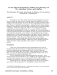
An overview of the available potentials is given in table 2 along with the arguments needed for each pair of
types.
2.1
Number of types
Previously there was a hard-coded limit to the maximum number of types, set to 16 by default. In RUMD 3.0
this limit has been removed, because parameters for potentials are now stored differently.
4
Gaussian core
Lennard–Jones Gaussian
Lennard–Jones (12,6)
Lennard–Jones (m,n)
Lennard–Jones (12,6)
Name of Potential
Dzugutov
IPL6/LN
Inverse Power Law, arbitrary n
Inverse Power Law, n = 18
Inverse Power Law, n = 12
Buckingham (exp,six)
5
Table 1: List of pair potentials implemented in RUMD.
Definition
Parameters/Constants
SetParams
ij )
v(r
6 12
σij
σij
4 · ij
ij , σij
(i, j, σij , ij , Rcut )
− rij
rij
n m
n o
σij
σij
ij
− m · rij
ij , σij , m, n
(i, j, σij , ij , Rcut )
(m−n) n · rij
12
6 σij
σij
ij
− 2 · rij
ij , σij
(i, j, σij , ij , Rcut )
rij
6
2 12
σij
σij
0
ij
− 2 rij
− 0 · exp − r−r
ij , σij , 0 , σ0 , r0
(i, j, σij , ij , Rcut , 0 , σ0 , r0 )
rij
2·σ0
2
−rij
ij · exp
ij , σij
(i, j, σij , ij , Rcut )
σij
h i
6
rij
rm
6
α
ij (α−6)
exp α 1 − rm
− (α−6)
ij , rm , α
(i, j, rm , ij , Rcut )
rij
12
σij
ij rij
ij , σij
(i, j, σij , ij , Rcut )
18
σij
ij rij
ij , σij
(i, j, σij , ij , Rcut )
n
σ
ij r ij
ij , σij , n
(i, j, σij , ij , Rcut , n)
6 ij −1
σij
r
ij rij
ln σij
ij , σij
(i, j, σij , ij , Rcut )
ij
c
d
−n
A · r − B exp rij −a + B · exp rij −b
A, B, a, b, c, d
(i, j, A, B, a, b, c, d)
Pot_Dzugutov
Pot_IPL6_LN
Pot_IPL_n
Pot_IPL_18
Pot_IPL_12
Pot_Buckingham
Pot_Gauss
Pot_LJ_12_6_Gauss
Pot_gLJ_m12_n6
Pot_gLJ_m_n
Pot_LJ_12_6
Name in code
2.2
Cut-offs
For almost all pair potentials the constructor takes a required argument cutoff_method which is one of
rumd.ShiftedPotential, rumd.ShiftedForce or rumd.NoShift. The traditional choice is shifted-potential,
but in our group we use shifted-force cutoffs more and more. Note that neither the cut-off method nor the cut-off
distance may be specified for Dzugutov potential, which has an exponential cut-off built into the potential itself.
2.3
Attaching potential objects to the simulation object
For a simple system with a single pair potential, one typically uses rumd.SetPotential(pot), where pot is
the potential object. If the total potential involves combining more than one potential object then one should
use AddPotential (although SetPotential can still be used for the first one—the difference is that the list
of potentials is reset when SetPotential is used). Potentials for intra-molecular forces (bond, bond-angles,
and dihedral angles) are not attached by these methods, but rather via the special methods SetBondConstraint,
SetBondFENE, SetBondHarmonic, SetAngleCosSq, SetDihedralRyckaert; the reason has to do with exclusions—
one often wants to exclude non-bonded interactions between bonded atoms. These methods will be described
in Section 5.
2.4
General methods for pair potentials
SetParams(...) Set the parameters for a given pair of types (described in the tutorial). The exact arguments
depend on the pair potential. To find out what they are within python, type rumd.Pot_LJ_12_6.SetParams)
(for example). Typically the first two arguments are the two types i and j involved in a given interaction.
New in version 2.1 is that Newton’s third law is assumed by default, so only it is no longer necessary to
call SetParams both for types 0 and 1 and then 1 and 0, say.
SetID_String(pot_str) Set the string which identifies a potential (in for example the energies file if the
potential is being computed in addition to the actual simulation potential, or is one term of the latter).
GetID_String() Get the ID string for this potential.
SetVerbose(v) If v is false, messages to standard output are suppressed.
SetNbListSkin(skin) Set the skin for the neighbor list (the width of the extra shell of neighbors which allow
some time steps to be taken before re-building).
GetNbListSkin() Get the skin for the neighbor list.
SetAssumeNewton3(bool assume_N3) Pass False to disable symmetric interactions between unlike types by
default. Pass True to enable (default: True).
GetPotentialEnergy() Return the potential energy contribution from this pair potential. This will cause a
kernel launch; it does not use the results from a previous call to CalcF.
WritePotentials(simBox) Write the pair potentials and pair forces (for all type-combinations) to a file (whose
name consists of potentials_ plus the ID string, with a .dat extension). A simulation box is passed so
that the appropriate range of r values is known. It is more convenient, however, to call WritePotentials
method in rumdSimulation, which will call it on all attached pair potentials and automatically pass the
simulation box.
SetNbListDesortingDrift(desorting_drift) Change the assumed value of the maximum drift of a particle
between sorting. This is only relevant for large systems where memory use by the neighbor list is being
6
optimized. The default value is 2.0. When trying to maximize the system size that can be run on a given
card, a smaller value could be set2 .
3
3.1
Other potentials
TetheredGroup
This potential allows you you identify a group of particles which are to be “tethered” to a set of so-called “virtual
lattice sites” by harmonic springs. The particles are currently identified by type: A list of types is passed to
the constructor, and all particles are those types are considered part of the group3 . The spring constant is
the same for all particles in the group, and the virtual lattice sites can be displaced using the Move function
(typically inside a method to be called using the “run-time action” mechanism (see section 10.2); this can be
used to implement constant-speed boundary-driven shearing, for example.
potWall1 = TetheredGroup(solidAtomTypes=[0], springConstant=500.0)
sim.AddPotential(potWall1)
potWall1.SetDirection(2) # z direction (default is 0 ie x)
potWall1.Move(0.1) # move the virtual lattice sites a common amount
4
Integrators
This section provides details on the available integrators listed in the RUMD tutorial.
4.1
IntegratorNVE, IntegratorNVT
IntegratorNVE realizes Newtonian NVE dynamics via the Leap-frog algorithm whereas IntegratorNVT realizes
Nose-Hoover NVT dynamics [S. Nose, J. Chem. Phys. 81, 511 (1984)]. The implementation of the Nose-Hoover
NVT dynamics is detailed in [S. Toxvaerd, Mol. Phys. 72, 159 (1991)]. In this implementation, the Leap-frog
algorithm naturally appears by setting the thermostat variable to zero. The former two integrators are thus
based on the same common C++ class IntegratorNVT where IntegratorNVE is simply a wrapper for this class
with fixed parameters. Examples of use may be found in the tutorial but are also listed below. Nose-Hoover
NVT dynamics can be run with
# Nose-Hoover NVT dynamics with time step dt = 0.0025 and temperature T = 1.0
itg = rumd.IntegratorNVT(timeStep=0.0025, targetTemperature=1.0)
The relaxation time of the thermostat can be controlled with
itg.SetRelaxationTime(0.2)
A linear temperature ramp can also be associated with the NVT dynamics via
itg.SetTemperatureChangePerTimeStep(0.01)
2 It is important to ensure that then sorting happens frequently enough that this limit is not exceeded—the program will
terminate if the allocated memory turns out to be insufficient due to “desorting drift”. The autotuner is not yet smart enough to
handle these situations automatically.
3 This typically means that extra types have to be introduced which are otherwise identical to existing types, just for identifying
sets of particles for tethering. A more general particle selection mechanism will be implemented in a future version.
7
This causes targetTemperature to be changed every time step with ∆T = 0.01 until the simulation is complete.
Alternatively, Newtonian NVE dynamics can be run with
# Newtonian NVE dynamics with time step dt = 0.0025.
itg = rumd.IntegratorNVE(timeStep=0.0025)
Note: No correction of the energy E is performed, and round-off errors will eventually cause the energy to drift
over a long simulation. One should always estimate whether this drift is significant for the phenomena under
investigation.
4.2
IntegratorNVU
This is a new molecular dynamics that instead of conserving the energy E (as in Newtonian dynamics) conserves
the total potential energy U . NVU dynamics traces out a geodesic curve on the so-called constant-potentialenergy hypersurface Ω, given by (R ≡ (r1 , ..., rN ))
Ω = {R ∈ R3N | U (R) = U0 },
(1)
in which U0 is a constant. More details on the dynamics and its implementation can be found in T. S. Ingebrigtsen et al., J. Chem. Phys. 135, 104101 (2011); ibid. 135, 104102 (2011); ibid. 137, 244101 (2012). Examples of
use are given below
# NVU dynamics with (mass-weighted) step size in 3N-dimensional
# configuration space dispLength = 0.01 and potentialEnergyPerParticle = -1.0
itg = rumd.IntegratorNVU(dispLength=0.01, potentialEnergyPerParticle=-1.0)
NVU dynamics gives equivalent results to NVE dynamics for most properties, and potentialEnergyPerParticle
could, for instance, be chosen as the average potential energy of a given state point. There is no drift of the
potential energy as this is explicitly corrected by the implementation. dispLength (also known as l0 ) is similar
to the time step ∆t of NVE dynamics and cannot be chosen arbitrarily large.
4.3
IntegratorSLLOD
This integrator uses the SLLOD equations of motion are used to simulate simple shear flow. The flow is in the
x-direction with a gradient in the y-direction; that is, the further you go in the (positive) y-direction, the faster
the streaming velocity (in the positive x-direction). As is typically done we use an isokinetic thermostat, which
keeps the kinetic energy constant. Our implementation is based on Pan et al., “Operator splitting algorithm
for isokinetic SLLOD molecular dynamics”, J. Chem. Phys., 122, 094114 (2005), and conserves the kinetic
energy to a high precision. Note that while RUMD in general is coded in single precision, parts of SLLOD are
done in double precision. These include the kinetic energy-like quantities which are summed for the isokinetic
thermostat. In addition the incrementing of the box-shift is done in double precision on the host in order to
allow small strain rates.
This integrator requires a simulation box that implements a special kind of periodic boundary conditions, socalled Lees-Edwards boundary conditions, implemented using LeesEdwardsSimulationBox. Here is the Python
code for running a SLLOD simulation:
sim = rumdSimulation(...)
# create a Lees-Edwards box based on the existing box
# (can be omitted if using a configuration that came from a
# SLLOD simulation)
le = rumd.LeesEdwardsSimulationBox(sim.sample.GetSimulationBox())
8
sim.SetSimulationBox(le)
# strain rates below 1.e-6 may not be stable for small box sizes (the box-shift
# per time step must not be swallowed by round-off error)
itg = rumd.IntegratorSLLOD(timeStep=0.004, strainRate=1.e-5)
sim.SetIntegrator(itg)
# T is the desired temperature; N the number of particles
# -3 due to momentum conservation
# (perhaps should be -4 because of the kinetic energy constraint)
itg.SetKineticEnergy(0.5*T*(3*N-3.))
# xy is the relevant component of the stress (from version 3.0 includes kinetic contribution by default)
# for stress-strain curves, determining viscosity, etc.
sim.SetOutputMetaData("energies", stress_xy=True)
sim.Run(...)
Note that the analysis tools that analyze configurations (such as rumd_rdf and rumd_msd) correctly handle
the Lees-Edwards boundary conditions. It is important to realize, however, that the rumd_msd only considers
displacements transverse to the shearing (x) direction.
4.4
IntegratorMolecularSLLOD
The above integrator, IntegratorSLLOD, is for use on atomic systems. It can be used with molecular systems,
but there are some issues which arise with such systems, in particular to do with the thermostatting mechanism.
To avoid these issues there is a separate integrator class, IntegratorMolecularSLLOD, which integrates the
molecular formulation of the SLLOD equations of motion. The essential difference is that (1) the streaming
velocity used to adjust the changes in position and momentum is evaluated at the center of mass of the molecule
containing that atom, and (2) the thermostat constrains the kinetic energy associated with the molecular centers
of mass, leaving rotations and other degrees of freedom unthermostatted. The algorithm is a straightforward
generalization of the one of Pan et al that was used for the atomic case. Use of IntegratorMolecularSLLOD is
exactly as for IntegratorSLLOD; note that it will give an error if no molecules have been defined (section 5).
4.5
IntegratorIHS
Potential energy minimization is performed with IntegratorIHS
via Newtonian dynamics (Leap-frog algoP
rithm). A path is followed in configuration space where i Fi · vi > 0. If the latter sum becomes negative vi
is set equal to zero for all particles i. A simulation is run with
# timeStep specifies the time step of Newtonian dynamics
itg = rumd.IntegratorIHS(timeStep=0.0005)
The timeStep should be chosen smaller than usual MD simulations. After setting the integrator on the simulation object one can call Run(...) in the usual way to integrate for a fixed number of steps. A more typical
mode of use is to run until some convergence criterion has been reached. Moreover, it is also typical to be
running an ordinary MD simulation, and periodically make a copy on which energy minimization is performed.
This can be done by using the IHS_OutputManager class, described in Section 6.5, which acts as a wrapper
around IntegratorIHS.
9
4.6
IntegratorMMC
IntegratorMMC implements the Metropolis algorithm for canonical ensemble Monte Carlo simulations [N.
Metropolis et al., J. Chem. Phys. 21, 1087 (1953)]. The integrator applies cubic-shaped all-particle trial
moves and uses a random-number generator suitable for running efficient simulations on the GPU [GPU Gems
3, Chapter 37]. The integrator may be invoked with
# canonical ensemble Monte Carlo simulations
# dispLength = 0.01 is the sidelength of cubic trial displacements
# all particles are moved at once
itg = rumd.IntegratorMMC(dispLength=0.001, targetTemperature=1.0)
The acceptance rate of the MC algorithm can be extracted via
sim.Run(...)
# a magic number for the acceptance rate is 50%
ratio = itg.GetAcceptanceRate()
print "MC acceptance ratio: " + str(ratio)
5
Molecules
The setting up of simulations involving molecules is described by a basic example in the tutorial. Here we add
some further details about the intra-molecular potentials and about how to set up position and topology files
for a mixture of molecules.
5.1
Potentials for bonds, bond angles, dihedral angles
The potential describing intra-molecular interactions in RUMD contains three terms: one for bonds, one for
bond angles and one for dihedral angles. The bonds can be described either by a harmonic potential or by the
Finite Extensible Nonlinear Elastic (FENE) potential. The potential for harmonic bonds reads:
Ubond (~r) =
1 X (i)
(i)
ks (rij − lb )2 ,
2
(2)
bonds
(i)
(i)
where ks is the spring constant of bond type i and lb its zero force bond length. The potential for bond
angles is given by:
1 X (i)
Uangle (~r) =
kθ [cos(θ) − cos(θ(i) )]2 ,
(3)
2
angles
(i)
kθ
(i)
where
is the angle force constant for angle force type i and θ0 the zero force angle. The parameters for the
harmonic bond and bond angle potentials come from the Generalized Amber Force Field (GAFF) in Wang et
al., “Development and testing of a general amber force Field”, J. Comp. Chem., 25, 1157 (2004). The potential
for the dihedral angles have the following form:
Udihedral (~r) =
5
X X
n
c(i)
n cos (φ),
(4)
dihed n=0
(i)
where cn are the torsion coefficients for torsional force type i. The parameters for the dihedral angle potential
come from Ryckaert et al., “Molecular dynamics of liquid alkanes”, Faraday Disc. Chem. Soc., 66, 95(1978).
10
The FENE potential can also be used to describe bonds. It is given by:
"
2 #
1 2 X
rij
U (~r) = − kR0
ln 1 −
,
2
R0
(5)
bonds
where k = 30 and R0 = 1.5 (in reduced units). At the moment the constraint method is applicable for molecules
with few constraints.
Here is a typical python code for setting up the intra-molecular potential:
[set up simulation object and add non-bonding potentials as usual]
# read topology file
sim.ReadMoleculeData("start.top")
# create intramolecular potential object
sim.SetBondHarmonic(bond_type=0, lbond=0.39, ks=2700)
sim.SetAngleCosSq(angle_type=0, theta0=2.09, ktheta=537)
sim.SetAngleCosSq(angle_type=1, theta0=1.85, ktheta=413)
sim.SetDihedralRyckaert(dihedral_type=0, coeffs=[0, 133, 0, 0, 0, 0])
sim.SetDihedralRyckaert(dihedral_type=1, coeffs=[0,-133, 0, 0, 0, 0])
sim.SetDihedralRyckaert(dihedral_type=2, coeffs=[15.5000, 20.3050, -21.9170, \
-5.1150, 43.8340, -52.6070])
Note that there can be as many bond-, angle- and dihedral- types as wished. The function SetDihedralRyckaert
(i)
(i)
has two arguments: the dihedral angle type i and the values of the torsion coefficients from c0 to c5 . The
way to obtain the topology file start.top used above will be described in section 5.4 below.
5.2
Constraints on bond lengths
As an alternative to using intra-molecular potentials, molecules can be simulated using constraints, whereby a
fixed distance between two particles is maintained via a constraint force. The actual implementation is described
in [S. Toxvaerd et al., J. Chem. Phys. 131, 064102 (2009)]. The procedure for setting up a rigid bond between
two particles is analog to adding a bond potential between the two particles, i.e.,
# the distance between all bonds of type = 0 is lbond = 0.584
sim.SetBondConstraint(bond_type=0, lbond=0.584)
The constraint forces are calculated by solving a set of non-linear equations. This is achieved by first making
them linear and thus involves iteration. The number of times the linear set of equations is iterated can be
controlled with
# iterate the linear set of equations 5 times
sim.moleculeData.SetNumberOfConstraintIterations(5)
The more iterations the more costly the algorithm becomes. Since there is no convergence check, one should
verify that the bond lengths are satisfied to within the desired tolerance via
sim.Run(...)
# prints the standard deviation of all constrained bond lengths
# with respect to the lbond values
sim.WriteConstraints()
11
A good value for the standard deviation would be less than 10−5 − 10−6 . Due to an internal constraint on the
linear equation solver, there may not be more than 512 constraints (fixed bonds) per molecule. This will be
lifted in a future RUMD release. It should also be noted that for each bond constraint; 1 degree of freedom
is naively removed (for the purpose of evaluating the kinetic temperature). The implementation does not try
estimate whether the system is, for instance, over-specified.
For linear molecules, for instance chain molecules without side groups which are often used as course-grained
models for polymers, an optimized linear solver has been implemented. This solver can be chosen by calling
# use optimized solver for linear molecules with constraints
sim.moleculeData.SetLinearConstraintMolecules(True)
after setting the constraints. This optimization is possible because the system of linear equations for a linear
molecule has a simple tridiagonal shape. For this optimized solver to work properly, the bonds in the topology
file have to be ordered. Moreover, since the same solver is used for all molecules in the simulation, the solver
only gives correct results if all molecules containing constraints are linear. This optimization has not been
tested for a large range of molecule sizes, but for Lennard-Jones chains consisting of 9 constraint bonds, the
simulation time is about 70% of the default linear solver time.
5.3
The topology file
An example of topology file can be found in the subdirectory Conf/Mol. It is called mol.top. It is a simple
text file which specifies the bonds between the atoms. To define the bonds in a .top file we:
1. Specify the beginning of the bond section with the keyword
[ bonds ]
We will call this a section specifier.
2. Add a comment line starting with ;, for example,
; My bonds
3. Specify the bonds. Each bond is described row-wise using four positive entries which are all integers: (i)
The first entry is the the molecule index, (ii) the second and third integers are the indices of the particle
forming the bond and (iii) the forth integer sets the bond type. This means that if atom 42 is bonded
with 55 in molecule 2 with bond type 5 we write
2 42 55 5
and so forth.
Likewise for angles. Here the section specifier is [ angles ] and five entries are needed to specify the angle.
The first again indicates what molecule this angle belongs to and the last specifies the angle type. For example,
if atom with index 42 is the vertex of the angle and atoms 55 and 78 are the two end-points we can use
2 55 42 78 0
This angle is found in molecule with index 2 and is of type 0. As you might have guessed, to specify a dihedral
angle you need 6 entries since a dihedral is defined via three bonds. The section specifier is [ dihedrals ].
Here is a simple example on how to write a topology file of a single butane molecule based on a unitedatomic-unit model, where the methyl (the two CH3 groups) and methylene (the two CH2 groups) are represented
by a single particle:
12
[
;
0
0
0
bonds ]
Bond section - ks = 311 kcal/mol lb = 3.4 ?~E
0 1 0
1 2 0
2 3 0
[
;
0
0
angles ]
Angle section - ktheta = 63.7 kcal/(mol rad**2) theta0 = 109 degr.
0 1 2 0
1 2 3 0
[ dihedrals ]
; dihedral/torsion section - RB coefficients
0 0 1 2 3 0
5.4
Tools for setting up position and topology files
Writing position (.xyz) and topology (.top) files from scratch for a mixture of molecules can be a lot of work
and it is very error prone to type in all the information. Fortunately, RUMD provides some useful tools to do
that from the position and topology files of single molecules. At the moment these tools are:
rumd replicate molecules Specify a .top file for a single molecule and a corresponding .xyz file for the
constituent atoms and this program will make copies of the molecules and put them on a lattice with
appropriate spacing. Note that this will typically be a very low density system and you will need to
compress the simulation box in order to have the right density.
rumd sfg This program allows you to setup the configuration for a molecular system (including molecular
mixtures) from .xyz and .top files for the individual molecules. The files start.xyz.gz and start.top
are written and can be used as start files. Usage:
sep_sfg <m1.xyz> <m1.top> <num1> <m2.xyz> <m2.top> <num2> ...
m1.xyz: .xyz file for the atoms in molecule one (string).
m1.top: the topology file for molecule one (string).
num1: the number of molecules of this type (integer).
and so forth.
The molecules’ center-of-mass are positioned on a low density simple cubic lattice, and you will probably
need to compress your system.
Example
Assume you wish to simulate a system composed of 200 FENE molecules with 5 beads in each. You can write
the single-molecule topology file as:
[
;
0
0
0
0
bonds ]
Single FENE chain
0 1 0
1 2 0
2 3 0
3 4 0
13
We here let both the molecule index and the bond type be 0, but they need not to be. Save this file as, for
example, single_fene.top
To specify the relative positions of the beads in the molecule we can write a single-molecule .xyz file
5
Single FENE
0 0 0 0
0 0 0 1
0 0 0 2
0 0 0 3
0 0 0 4
This corresponds to a simple linear chain. Save the .xyz file as single_fene.xyz, for example. To replicate
the molecule 200 times we type
./rumd_replicate_molecules single_fene.xyz single.top 200
This command produces two files called start.top and start.xyz.gz with all the information needed to start
a simulation. However, as mentioned above the density of the system is probably not correct. To compress and
equilibrate the system, you can. . .
2
6
Output
The core of a molecular dynamics is the algorithm, which needs to be as fast as possible. But the algorithm
is useless without output, and the more control a user has over the output the more useful the software. An
additional consideration is that with a very fast code one has to be careful not to drown in data, particularly
where configurations are concerned. We use so-called output managers to control both how frequently a given
kind of data is written (scheduling) and precisely what data is included in the files (called the meta-data, a
specification of what data is in a given output file).
6.1
Output managers
Output is controlled by output managers. These are software components (classes) written in C++ or Python
which manage the writing of various observables to files. A given output manager manages writing of data to
one output file at a time, for example one containing energy-like quantities (energies file), or one containing
configurations (trajectory file). The basic output managers are written in C++ but can of course be controlled
using the Python interface. The mechanism for handling Python output managers exists in order for users to be
able to write their own run-time analysis code in Python without having to recompile the main RUMD software
(i.e. the C++ library).
We start by discussing the C++ output managers, in particular the so-called energies output manager and
trajectory output manager. In order to avoid data corruption in the event of a long simulation being interrupted,
for the purposes of output the simulation run is divided into output “blocks”. The output manager starts a
new file each time a new block is started, with an incremented block index, thus energies files have names like
energies0000.dat.gz, energies0001.dat.gz, etc. and trajectory files have names trajectory0000.xyz.gz
etc. (previously, up to version 2.0, block0000.xyz.gz: old data is still be readable). Note that the files
are written in ASCII to be human readable but then compressed using gzip. These files reside by default in
the directory TrajectoryFiles, but for standard analysis and post-processing it is not necessary to be aware
of them (the analysis tools know where to find them). On the other hand it is straightforward to make a
concatenated uncompressed energies file using zcat TrajectoryFiles/energies* > energies.dat if needed.
14
The uncompressed file will take up 2-3 times as much disk space as the compressed ones did. As much as
possible, analysis scripts should also read directly the compressed files (in Python this is easily done using the
gzip module) rather than requiring the user to separately uncompress the files.
The output files appear in the directory TrajectoryFiles by default. If this directory exists it is renamed
with a .rumd_bak extension (if the latter exists it is overwritten). From version 2.1.1 on it is possible to disable
backup by calling sim.sample.EnableBackup(False). Changing the output directory is done as follows:
sim.SetOutputDirectory("TrajFilesRun01")
Data files in general should be self-describing; in particular it should be possible to look at the file and know
what each column represents. We implement this principle in both energies and trajectory files. Analysis
programs should make use of the provided meta-data instead of expecting a certain order of columns.
If not explicitly set by the user via sim.SetBlocksize(), the block size will be chosen automatically when
sim.Run() is called, such that the number of blocks is of order 100-1000 and the block size a power of 2.
6.2
Log-lin scheduling: Linear, logarithmic, and mixed.
The output managers can save items (configurations to a trajectory file or lines to an energies file) at equally
spaced intervals (linear saving), logarithmically spaced (in powers of two, plus the zeroth) or a “mixed” scheduling called log-lin. The scheduling for a given output manager is set via
SetOutputScheduling(manager, schedule, **kwargs)
which was described in the tutorial. The manager argument is the name of an output manager, for example
“trajectory” or “energies”. The schedule argument is one of “linear” (which requires a following keyword
argument interval), “logarithmic” (which can take an optional following keyword argument base), “none”,
or “loglin” (which requires keyword arguments base and maxInterval). Since “linear” and “logarithmic”
scheduling are special cases of “loglin”, let us consider the meaning of the parameters base and maxInterval:
base This is the smallest interval of time steps considered. All intervals between writing items are multiples of
base.
maxInterval The largest interval allowed between saves. Its purpose is to allowed combined linear and logarithmic saving. It should be set to zero to do pure logarithmic saving. If non-zero, the interval between
writes will, after increasing initially logarithmically, become fixed at maxInterval.
Some possible combinations are, assuming blockSize=128:
Pure logarithmic saving with base 1 Set base=1, maxInterval=0, and you get time steps 0, 1, 2, 4, 8, 16,
32, 64, 128 within each block. This is equivalent to “logarithmic” scheduling without specifying base.
Pure linear saving at interval 4 time steps Set base=4 and maxInterval=4 and you get time steps 0, 4,
8, 12, 16, . . . , 128. This is equivalent to “linear” scheduling with interval=4.
“log-lin” Set base=1 and maxInterval=8, and you get time steps 0, 1, 2, 4, 8, 16, 24, 32, 40, 48, 56, . . . , 128.
Note the following restrictions on the values of base and maxInterval: When maxInterval is non-zero it must
be a multiple of base. Except for the case of linear saving (base=maxInterval), both base and maxInterval must
divide evenly into blockSize.
The meta-data in the comment line of a trajectory file contains an item timeStepIndex which gives the
number of the time step within the output block and a string which looks like logLin=0,10,0,4,10. The
five items in this list identify both the parameters of a particular log-lin saving scheme and the indexing of the
current time step with that scheme. It can be useful occasionally to understand these parameters. A description
of each one follows, in the order they appear in the string:
15
block Identifies which output block we are in. Will therefore be the same for all items written in a given block.
base Smallest interval of time steps considered. It does not change during a simulation run, but is a parameter
controlled (perhaps indirectly) by the user.
index Labels items within a block, in that it starts at zero and increments by 1 for each item written. When
maxInterval is set to zero (pure logarithmic saving), there is a simple relation between index and nextTimeStep: nextTimeStep = 0 if index = 0 and nextTimeStep = base × 2index-1 otherwise. Note that
the block size is given (again for pure logarithmic saving, maxInterval=0) by base ×2maxIndex-1
maxIndex The value of “index” for the last item in the block. So if the saving scheme is such that there are
8 items per block, maxIndex will have the value 7 (since index starts at zero). Does not change during a
simulation run4 ; is set based on parameters specified by the user.
maxInterval The largest interval allowed between saves. This is a user parameter which does not change.
There is a more complicated relation between nextTimeStep and index in this case.
6.3
Trajectories and energies
Trajectory and energy files are the primary output of RUMD, so it is worth describing them in some detail.
Trajectory files contain configurations, including the types and positions of all particles, and optionally their
velocities, forces, and other quantities. Energy files consist of one line of output for a given time step, which
lists global quantities, such as the total potential energy, or pressure, or a component of the stress tensor. To
keep track of potential changes in the formats for these files there is a format tag ioformat which appears in
the meta-data (first line of each file). The current value of ioformat is 2. The difference between ioformat
1 and 2 involves changes in the meta-data for trajectory (configuration) files. The software and analysis can
handle either format transparently.
Controlling what gets written, and the precision, in the energies and trajectory files is done via SetOutputMetaData
as described in the tutorial. One can specify more than one variable in a given call, for example:
sim.SetOutputMetaData("energies", totalEnergy=False, stress_xy=True)
A look at the first few lines of an output file (using zcat TrajectoryFiles/energies* | head, for example)
shows the meta-data. For the energies file and default settings, it might look like the following:
# ioformat=2 N=1000 Dt=0.005000 columns=ke,pe,p,T,Ps,Etot,W
0.78297 -6.92308 3.65423 0.522503 0 -6.14011 2.52269
0.779256 -6.9193 3.66705 0.520024 0 -6.14004 2.53585
0.77511 -6.91508 3.68272 0.517257 0 -6.13997 2.55168
...
The comment line contains the meta-data, including here the ioformat, time interval between lines (for
energies files one typically uses linear saving), number of particles (useful for analysis) and the list of symbols
identifying the columns. It is not a good idea to rely too much on a particular order of columns; when writing
an analysis script in Python for example, it is recommended to read the meta-data and extract the column
information so that the potential energy column, for example, is always correctly identified.
For trajectories, we use an extended xyz format, and a given file will contain all the trajectories from one
output block. For logarithmic saving this will be a relatively small number of configurations, less than 20.
Each configuration starts, as is usual with the xyz format, with the number of particles. The line following is
considered a comment line in the xyz format. We use it to write the meta-data. This can include information
4 The
exception to this is linear saving where the interval does not evenly divide the blockSize.
16
Table 2: Identifier and column-label for the main quantities that can be written to the energies file. For extensive
quantities, such as potential energy or virial (though not volume), the “per-particle” value is written.
identifier
potentialEnergy
kineticEnergy
virial
totalEnergy
temperature
pressure
volume
density (a)
thermostat_Ps (b)
enthalpy
stress_xx(c)
stress_yy
stress_zz
stress_xy
stress_yz
stress_xz
v_com_x
v_com_y
v_com_z
potentialVirial (d)
constraintVirial (d)
simulationDisplacementLength
instantaneousTimeStepSq (e)
euclideanLength (e)
(a)
column label
pe
ke
W
Etot
T
p
V
rho
Ps
H
sxx
syy
szz
sxy
syz
sxz
v_com_x
v_com_y
v_com_z
pot_W
con_W
(e)
dispLength
dt^2
eclLength
From version 2.1 on.
The extra degree of freedom used by the NVT
integrator.
(c)
Versions before 3.0 did not include the kinetic contribution to the atomic stress by
default.
Change using (Sample method)
SetIncludeKineticStress(bool).
Contributions to the atomic stress from bond-constraints,
angle- and dihedral-forces are not included.
(d)
potentialVirial : contribution to virial from
the potential; constraintVirial : contribution
to virial from constraints.
(e)
Parameters associated with NVU dynamics
(IntegratorNVU)
(b)
17
about the simulation such as the simulation box and the integrator (including whatever parameters are needed
to restart a simulation), the time step and log-lin parameters and a list of symbols identifying the columns.
It can sometimes be necessary to look at the configuration file (for example in order to check the number of
particles or the box size). Here is an example:
1000
ioformat=2 timeStepIndex=0 logLin=0,10,0,4,10 numTypes=2 integrator=IntegratorNVE,0.005 \
sim_box=RectangularSimulationBox,9.41,9.41,9.41 mass=1.0000,1.0000 \
columns=type,x,y,z,imx,imy,imz,pe,vir
0 4.6021 0.1670 3.7406 0 0 0 -7.4641 13.2556
0 -0.2562 -4.1929 4.5378 0 0 0 -6.9324 7.1333
0 -3.2822 2.1659 1.1286 0 0 0 -7.2647 15.1471
The columns labelled imx etc., give the image indices—what multiple of the box size must be added in a
given direction to give the total displacement taking into account the number of times a periodic boundary has
been crossed. It is essential for correct determination of mean squared displacement, for example.
6.4
External calculators: adding data to the energies file
In addition to including or excluding the standard energy-like quantities, it is possible to attach an “external
calculator” which knows how to calculate some quantity, and have that quantity be included in the energies file.
This can be more convenient than creating separate files for new quantities.
pot18 = Pot_IPL_n_18(...)
alt_pot_calc = rumd.AlternatePotentialCalculator(sample=sim.sample, alt_pot=pot18)
sim.AddExternalCalculator(alt_pot_calc)
The potential energy calculated by the IPL n = 18 potential will then appear in the energies files in the
column designated by the “ID string” of the potential. The latter can be obtained via pot18.GetID_String()
and changed via pot18.SetID_String(). Another external calculator calculates the hypervirial by numerical
differentiation. Doing the following
hypervirCalc = rumd.HypervirialCalculator(sample=sim.sample, delta_ln_rho=0.0005)
sim.AddExternalCalculator(hypervirCalc)
will cause columns labelled approx_vir and approx_h_vir to appear in the energies file.
These represent the finite difference approximations to the virial and hypervirial, respectively. The virial is
included in order to be able to compare it to the true virial as a check. The second argument to the constructor
of HypervirialCalculator is the change in ln(ρ) (approximately the same as the fractional change in density)
to be used for the finite difference calculation. Note: the above lines must appear after setting the potential!
6.5
Other output managers (C++)
An example of an additional output manager implement in C++ is one for computing inherent states (local minima of the potential energy function in 3N dimensions), using IHS_OutputManager. Here each time
the Update function is called, the sample configuration is copied and an energy minimization calculation
is run on the copy using the integrator IntegratorIHS (see Section 4.5). The energies are written to files
ihsEnergiesXXXX.dat.gz, while the minimized configurations are written to files ihsXXXX.xyz.gz.
ihs_man = rumd.IHS_OutputManager(sample=sim.sample, timeStep=0.005)
ihs_man.SetMaximumNumberIterations(5000)
ihs_man.SetIHSLinearWriteInterval(100)
18
#ihs_man.SetWriteIHS_Config(False) # turn off writing of minimized configurations
sim.sample.AddOutputManager(ihs_man)
Note that the interface has not been completely harmonized with the other output managers, in that a
method SetIHSLinearWriteInterval on the manager object is used to control how frequently energy minimizations are carried out, rather than using the SetOutputScheduling method of rumdSimulation. Similarly SetWriteIHS_Config sets whether the minimized configurations should be written or not (instead of
SetOutputMetaaData. Note also that the energy minimization algorithm has not been used very much and
probably could be improved, for example by using conjugate-gradient minimization to speed convergence near
the minimum. The use of single precision in RUMD is likely to limit the convergence, however.
6.6
Python output managers
Sometimes it is desirable to do data analysis during run-time. This is for instance the case when doing postproduction analysis would involve saving huge amounts of data. A python output manager is useful in this case,
since it allows so-called call-back functions to be added to the output manager, converting simulation data to
output.
To use a python output manager, a call-back function has to be defined. The call-back function should work
on the sample object, and return a string with the data, for instance:
def momentum(sample):
vel = sample.GetVelocities()
P
= sum(vel)
return "%4g %4g %4g " % (P[0], P[1], P[2])
Then a new python output manager can be made, and the call-back function should be added to it:
sim.NewOutputManager("analysis", outputDirectory="TrajectoryFiles")
sim.SetOutputScheduling("analysis", "linear", interval = 100, blockSize = 10000)
sim.RegisterCallback("analysis", momentum, header = "Px, Py, Pz, ")
This writes data files named analysis0000.dat.gz, analysis0001.dat.gz etc. to the same directory as the
other output managers.
Note that RegisterCallback() can be called multiple times on the same python output manager but with
different call-back functions. The output and header strings of the different call-back functions are concatenated
to a single line (do not use any end of line characters in these strings).
The scheduling of the python output manager is set in the same way as for the C++ output managers.
They do not enforce the block size to be the same, however (related to this, is that the restart mechanism does
not take account of Python output managers). To use a different block size for a python output manager, the
optional keyword argument blockSize can be used.
There is another (useful) difference between the python and C++ output managers: when the schedule of a
python output manager is set to “none”, it is necessary to specify an interval. The schedule “none” is for for a
python output manager the same as the schedule “linear”, with the difference that no output is written to files.
So the call-back functions that have been added to the python output manager are still called on the specified
time steps. This is for instance useful for scaling the box or changing potential parameters step by step, or for
doing time averaging of simulation data.
The call-back function can get simulation data from the sample object. Useful functions on the sample
object include:
GetPositions(self) Returns the atom positions as a numpy array.
GetImages(self) Returns the atom images images as a numpy array.
19
GetVelocities(self) Returns the atom velocities as a numpy array.
GetForces(self) Returns the atom forces forces as a numpy array.
GetPotentialEnergy(self) Returns the total potential energy.
GetVirial(self) Returns the total virial.
A more extensive list of Sample methods is given in section 12.
7
Optimizing performance with the autotuner
The basic usage of the autotuner is described in the tutorial. It is convenient to distinguish between “user
parameters” and “internal parameters” (also called technical parameters). User parameters specify the kind of
simulation the user wants to run: the potential and its parameters, the integrator and its parameters (time step
and temperature for example), the number of particles (also of each type) and the density. The type of graphics
card is also considered a user parameter, though it is not necessarily something the user can choose explicitly.
The autotuner’s task is to find the optimal technical parameters for a given set of user parameters. After the
call to Tune the simulation object is left in the same state as before, but the internal parameters have been
set to the optimal values, which are also written to the file autotune.dat. If the file exists already when the
autotuner is run, it is checked to see if the user parameters match the current ones. If so, the optimal technical
parameters are read from the file instead of going through the autotune-process again. (Note that a different
GPU type is sufficient to cause the autotuner to run again.)
7.1
Technical parameters determining performance
Here is a description of the technical parameters optimized by the autotuner, mentioning also their default
values and how they can be set “manually” by the user.
pb The number of particles per thread-block, for neighbor-list generation, force calculation and integration
step, default value 32. A value for pb can be specified by the user as a constructor argument to
rumdSimulation: sim=rumdSimulation("start.xyz.gz",pb=32), or set later (together with tp) via
sim.sample.SetPB_TP(pb, tp).
tp The number of threads per particle, default value 4, for neighbor-list generation and force calculation (not
integration). The total number of threads in a thread block is therefore pb times tp. It may also be
specified as a constructor argument to rumdSimulation or via sim.sample.SetPB_TP(pb, tp)
NB skin The thickness of the extra shell (beyond the maximum cut-off from the pair potential) searched when
constructing the neighbor list. Default value 0.3. If there is more than one pair potential then in principle
they could have different skin values, but it is not clear that this would be advantageous; the autotuner
enforces a common value. To manually change the skin use pot.SetNbListSkin(skin)
sorting scheme Whether to sort in 1 (X), 2 (XY) or 3 (XYZ) dimensions. The default scheme is XY which is
optimal for medium-to-large system sizes (for smaller sizes sorting scheme X is optimal, but XY is almost
as good). To set the sorting scheme manually do sim.sample.SetSortingScheme(rumd.SORT_X) for X
sorting, etc (the options are rumd.SORT_X, rumd.SORT_XY and rumd.SORT_XYZ).
sort-interval The number of time steps between sorting, default 200. Use sim.SetSortInterval(...) to
change. Setting the value to be 0 causes sorting to be disabled.
20
7.2
Fine control of the autotuner
It can be useful to keep one or more parameters fixed while tuning with respect to all the others. This is done
by passing keyword arguments to the constructor of the autotuner, such as
at = Autotune(pb=32, sorting_scheme="XY", ...)
For this purpose the names of the technical parameters need to match the variable-names used in the Python
script itself. They are: pb, tp, skin, sorting_scheme, sort_interval.
Another optional keyword argument is ignore_file=True, which will cause the autotuner to ignore an
existing file autotune.dat. In this case it will still (over-)write that file after the tuning process is complete.
8
Post-production analysis tools
The supplied tools are both stand-alone C++ programs that can be called from the command line, and (in many
cases) Python modules that can be imported into your script in order to do analysis on the fly (for example if
a script involves many simulations at different state points and the data is not otherwise needed afterwards one
can save disk space by doing the analysis after each state point.) Use of the most important tools was described
in the tutorial, although not all details were given. Here we give a more complete description of their options
and output files. There are is not complete harmony of different tools; the “common” options listed below are
not available on all tools, for example. There should be some kind of convergence in later versions of rumd.
The output files generally start with a comment line which identifies the columns, unless otherwise specified.
8.1
Common command-line options
Help -h gives a list of options for the tool. For example
[bead30] ~%rumd_rdf -h
Usage: rumd_rdf [-n <number of bins>] [-m <minimum time between configurations>]
[-f <first_block>] [-l <last_block>] [-v <verbose>] [-d directory]
[-e <writeEachConfig>] [-p <particles per molecule>]
Restricting to part of the simulation run Including -f 10 means data is read from block 10 onwards.
Including -l 20 means data from blocks after block 20 will not be read.
Non-standard output directory If data is not in the default directory TrajectoryFiles (either because
it’s been renamed or because SetOutputDirectory was used to change it from the start), use the -d <dir>
command-line option to specify where the analysis program should look for the data
Verbosity Including -v 1 allows various messages to be written to standard output. -v 0 (the default)
disallows (non-essential) output.
Molecular quantities In some tools calculating structural and dynamical quantities, the number of particles
per molecule may (or must) be specified (by -p5 ). If this is greater than 1 (the default) then corresponding
structural and dynamical quantities for the molecular center of mass are also computed.
5 For
some tools -m was previously used for this.
21
9
9.1
List of analysis tools
Analysis of the trajectories
rumd_rdf Compute time averaged radial distribution function. Usage:
rumd_rdf [-n <number of bins>] [-m <minimum time between configurations>]
[-f <first_block>] [-l <last_block>] [-v <verbose>] [-d directory]
[-e <writeEachConfig>] [-p <particles per molecule>]
Output file: rdf.dat, whose first column is the pair-distance r, with subsequent columns giving g(r) for
all pair combinations of atom types; for example if there are two types, then the columns are r, g00 , g01 ,
g10 , g11 (note g01 = g10 ). If the option -e 1 is specified, then a separate rdf file for each configuration is
written. The comment line in rdf.dat gives the concentrations of the different atom types. The range of
r values is the box size in the x-direction
(but note that for a cubic periodic box of side L non-zero values
√
do not appear for r greater than L 3/2). A minimum (simulation) time (default 0) may be specified using
-m when configurations have been saved logarithmically in order to reduce processing time and avoid too
closely spaced configurations receiving too much weight in the average.
rumd_msd Basic dynamical correlation functions: intermediate scattering function, mean-squared displacement,
non-Gaussian parameter. Usage:
rumd_msd [-h] [-m <particles per molecule>] [-f <first_block>]
[-l <last_block>] [-d directory] [-e <extra_times>] [-v <verbose>]
Note that a file qvalues.dat must be present, containing the q-value at which the self-intermediate
scattering function is to be calculated (one value for each atom type). New in version 2.1 is that the
restriction to configurations saved logarithmically has been relaxed. When the argument -e 1 is present,
the functions are evaluated more relative times (within a block), giving greater time resolution (but
possibly noisier curves). Output files: msd.dat (mean-squared displacement versus time for different
atom types), Fs.dat (self-intermediate scattering function versus time for different types ), FsSq.dat,
alpha2 (non-Gaussian parameter versus time for different types). Note that when Lees-Edwards boundary
conditions are present, only transverse displacements are included in the calculation.
rumd_sq Calculate the static structure factor by Fourier-transforming the radial distribution function in rdf.dat.
No attempt to handle the finite box-size, and hence integration range, intelligently is made; artifacts of
this (extra oscillations) are present in the output. Usage: rumd_sq <q_start> <q_final> <density>.
500 values of q ranging between the two user-supplied end-points are calculated. New in version 2.1
is handling an arbitrary number of types. Output files: Sq.dat (first column: q, subsequent columns:
SAB (q) for different pairs AB of types), qmax.dat (location of maximum of SAA (q) for each type A, can
be used as input to rumd_msd by renaming to qvalues.dat).
rumd_bonds (New in version 2.1.1) Compute bond length probability densities. Usage:
rumd_bonds [-h] [-n <number of bins>] [-m <minimum time between configurations>]
[-f <first_block>] [-l <last_block>] [-d directory] [-t topologyfile]
[-e <writeEachConfig>] [-v <verbose>]
Output file: bonds.dat, where the first column gives the bond lengths (the bins) and the rest of the
columns contain the probabilities of the bond lengths for each type of bond specified in the topology file.
The distributions have been normalized so that the surface under the distribution is 1. See rumd_rdf for
explanations of the other command line options.
22
rumd_rouse Calculate Rouse modes autocorrelation functions and the orientational autocorrelation of the endto-end vector of linear molecules. (see M. Doi and S. F. Edwards, The Theory of Polymer Dynamics,
Oxford Science Publications, 1986) Usage:
rumd_rouse [-h] [-m <particles per molecule>] [-f <first_block>]
[-l <last_block>] [-d directory] [-v <verbose>]
Output files: rouse_X0Xt.dat (autocorrelation functions of Rouse modes) rouse_X0X0.dat (variances
of Rouse modes) rouse_R0Rt.dat (orientational autocorrelation of end-to-end vector) rouse_R0R0.dat
(mean squared end-to-end vector and squared radius of gyration). Note that this analysis tool only gives
correct/meaningful output for systems with one kind of (linear) molecule. The data in the trajectory files
should be ordered such that the particle data are in the same order as the particles in the chain. (The
program does not read the topology file.)
rumd_visualize Load one configuration from each block into the molecular visualization program vmd.
9.2
Analysis of the energies
rumd_plot_energies Read data into xmgrace from the energies files as block data, and display one or more
columns. The purpose of the tool is to uncompress the energies files into a temporary ASCII file for
xmgrace to read. Command-line arguments are passed to xmgrace. At least one argument of the form
-bxy 0:2 is required to choose columns to be plotted (against each other, or as here, against line number).
rumd_stats Basic statistics (means, variances, covariances, drift) of the data in the energies files. Usage:
rumd_stats [-h] [-f<first_block>] [-l<last_block>] [-v <verbose> ]
[-d<directory>] [-b base_filename]
Written to standard output: total line count, then mean, variance and standard deviation for each column
of data in the energies files. Any columns in the energies files which are not among the “standard”
quantities, for example data computed by an external calculator, are flagged with a line “Non-standard
column identifier: ...”. Output files: energies_mean.dat (mean values), energies_var.dat (variances),
energies_mean_sq.dat (mean squared values, useful for combining data from independent runs to get
overall mean and variance), energies_covar.dat (covariances between all pairs of columns in the energies
files), energies_drift.dat (linear regression estimate of the linear drift of each quantity with respect to
line number; divide by the time interval between lines to get a proper rate). The option -b base_filename,
available from version 2.1.1, allows you to do basic statistics on a different set of files in the output directory.
They should be numbered like energies files, just with energies replaced by a different basename, and each
one should start with a comment line containing ”columns=a,b,c” to identify the columns.
rumd_autocorrelations Autocorrelation functions of the data in the energies files. Usage:
rumd_autocorrelations [-h] [-n] [-l <log_binning>] [-w <write_fraction>]
[-c <column_name> [<column_name> ...]]
The autocorrelation functions of all columns are calculated and saved to autocorrelations.dat.gz by
default. The first column of the output file contains the time. With the option -c column_name it
is possible to choose for which columns in the energies files to calculate the correlation function. The
name of the column as in the energies files should then be given. Only the first 0.01 fraction of the
autocorrelation is written to the output file by default to save space. It is possible to change this with
the -w write_fraction option. Another way to reduce the output file size is by performing logarithmic
23
data binning. This is done with the option -l log_binning, where the number of bins per decade should
be given. The option -n is used to normalize the autocorrelation with the variance, so it is unity at time
zero.
rumd_crosscorrelation A crosscorrelation function of two columns in the energies files. Usage:
rumd_crosscorrelation [-h] [-n] [-l <log_binning>] [-w <write_fraction>]
<column_name> <column_name>
The two names of the columns for which the crosscorrelation is calculated should be given. The names of
the columns will be used for the output file. The command rumd_crosscorrelation pe W for instance
will result in an output file with the name crosscorrelation-pe-W.dat.gz. The other command-line
options are the same as for the autocorrelations.
rumd_response Calculate the response function of one or two columns in the energies files. Usage:
rumd_response [-h] [-l <log_binning>] <column_name> [<column_name> ...]
One or two names of the columns should be specified. The response function is then calculated as the
Fourier transform of the derivative of the cross- or autocorrelation function. Again, the name(s) of the
column(s) will be used in the output file, so if one column name is given, for instance rumd_response pe
than the output file is response-pe.dat. By default, the data are smoothed with logarithmic data binning
with 20 bins per decade. To turn off data binning, write -l 0. The output file contains three columns
with the angular frequencies, the real parts, and the imaginary parts of the response function.
9.3
Calling analysis tools via the Python interface
Some of the analysis tools can be accessed within Python through the rumd_tools module. These are rumd_stats,
rumd_rdf and rumd_msd. Before the analysis tools can be called, it is necessary to make sure the relevant output
files are closed. This is done via sim.sample.TerminateOutputManagers(). Here is some example code for
rumd_stats
sim.Run(n_run_steps)
sim.sample.TerminateOutputManagers()
# create a rumd_stats object
rs = rumd_tools.rumd_stats()
rs.ComputeStats()
meanVals = rs.GetMeanVals()
meanSqVals = rs.GetMeanSqVals()
pressure = meanVals["p"] # the keys are the symbols in the file meta-data
pe = meanVals["pe"]
pe_var = meanSqVals["pe"] - pe**2
# to write the file that the command-line rumd_stats program writes:
rs.WriteStats()
# to print the stats summary to standard output:
rs.PrintStats()
and here is some code for rumd_rdf:
sim.sample.TerminateOutputManagers()
24
rdf_obj = rumd_tools.rumd_rdf()
# constructor arguments: number of bins and minimum time
rdf_obj.ComputeAll(1000, 100.0)
# include the state point information in the rdf file name
rdf_obj.WriteRDF("rdf%5.3f_%5.3f.dat" % (rho, T))
# to get as numpy array, first the r-values
rVals = rdf_obj.GetRadiusValues()
# and then the actual g(r) values for type 0-type 1 pairs
gVals = rdf_obj.GetRDFArray(type1=0,type2=1)
and for rumd_msd:
sim.sample.TerminateOutputManagers()
msd_obj = rumd_tools.rumd_msd()
msd_obj.SetQValues([7.25, 5.75]) # set qvalues (new in V2.1.1, otherwise
# reads from the file qvalues.dat)
msd_obj.SetExtraTimesWithinBlock # include extra time differences within
# an output-block (new in V 2.1.1; corresponds to -e argument)
msd_obj.ComputeAll()
# get a nDataPoints x 2 numpy array containing times and mean squared
# displacement values for particles of type 0
msd0 = msd_obj.GetMSD(0)
# get the intermediate scattering function for particles of type 0
isf0 = msd_obj.GetISF(0)
# get the non-Gaussian parameter alpha2 for particles of type 0
alpha2_0 = msd_obj.GetAlpha2(0)
msd_obj.GetChi4(0) # get the variance of the intermediate scattering
# for particle type 0 (new in version 2.1)
# write data to a file (all types)
msd_obj.WriteMSD("msd.dat")
msd_obj.WriteISF("Fs.dat")
msd_obj.WriteAlpha2("alpha.dat")
The module Python/analyze_energies.py (new in version 2.1.2) defines a class AnalyzeEnergies for
the analysis of the energies. Methods for the calculation of correlation functions and response functions are
implemented. The module also defines some generic functions for calculating correlation and response functions
of any 1D array. Some example code:
import analyze_energies as analyze
# Create analyze_energies object, read relevant columns from energy files
nrgs = analyze.AnalyzeEnergies()
nrgs.read_energies([’pe’, ’W’])
# calculate the normalized autocorrelation
time, auto = nrgs.correlation_function(’pe’, normalize=True)
# calculate the first 10% of the crosscorrelation
25
length = int(1.1 * len(nrgs.energies[’pe’]))
time, cross = nrgs.correlation_function(’pe’, ’W’, length=length)
# calculate response function
omega, response = nrgs.response_function(’W’, ’W’)
# Save correlation functions to file
import collections
output = collections.OrderedDict()
output[’time’] = time
output[’pe’] = auto
output[’pe-W’] = cross
analyze.write_columns_to_file("mycorrelations.dat.gz", output)
# Do logarithmic data binning on the response function and save to file
output = collections.OrderedDict()
bins = analyze.create_logarithmic_bins(omega[1], omega[-1], bins_per_decade=12)
binned_omega, binned_response = analyze.data_binning(omega, response, bins)
output[’omega’] = binned_omega
output[’real’] = binned_response.real
output[’imag’] = binned_response.imag
analyze.write_columns_to_file("myresponse.dat", output)
10
10.1
Additional features/tricks
Momentum resetting
Due to the inevitable numerical round-off error due to finite precision arithmetic (single precision in the case
of rumd), it is necessary to periodically reset the center of mass velocity to zero. By default this is done every
100 time steps. This interval can be changed via
sim.SetMomentumResetInterval(1000)
and turn off entirely by passing zero to the above method.
10.2
User defined run-time actions
New in version 2.1 is a facility for allowing users to include extra steps in the main integration loop. It operates
similar to python output managers in that the user supplies a function or bound method and specifies how
frequently it should be called. The method should not take any arguments so typically it will be a method
bound to an object of a Python-class defined in the user’s script, which contains references to the sample or
simulation or some other relevant object (such as a potential). For example if the sample should be gradually
compressed from a low density (this might be done to prepare a molecular configuration), then we could define
a class which has a reference to the sample object, and a method Compress, as follows
class Compressor:
def __init__(self, sample, scaleFactor):
self.sample = sample
self.scaleFactor = scaleFactor
def Compress(self):
self.sample.IsotropicScaleSystem(self.scaleFactor)
num_scale_intervals = 100
26
density_factor = rho_desired/rho_start
scale_factor = math.exp(-math.log(density_factor)/3/num_scale_intervals)
comp = Compressor(sim.sample, scale_factor)
scale_interval=1000
sim.SetRuntimeAction("compress", comp.Compress, scale_interval)
sim.Run(scale_interval * num_scale_intervals)
The run-time actions are called in order they were added, before the force calculation in the main loop. The
list always includes sorting the particles in memory and setting the total momentum to zero. Weak references
are used to store the list of run-time actions in order to allow them to refer to the sample or simulation object
without causing problems with circular references.
10.3
Changing the density
Here is a function that will change the simulation box in order to give a specified density.
def SetDensity(sim, new_rho):
# scale to get right density
nParticles = sim.GetNumberOfParticles()
vol = sim.GetVolume()
currentDensity = nParticles/vol
scaleFactor = pow(new_rho/currentDensity, -1./3)
sim.ScaleSystem(scaleFactor)
When simulating molecules, it might be more reasonable to keep the distances within the molecules fixed, for
instance when simulating rigid bonds. In this case, use the command sim.ScaleSystem(scaleFactor, CM=True).
10.4
Instantaneously scaling the velocities
When changing temperature abruptly in the simulation script, the thermostat will take some time to get the
average temperature to the right value. This can be circumvented by scaling the velocities instantaneously:
# Scale velocities from temperature Told to T
velocity_factor = ( T/Told )**0.5
sim.sample.ScaleVelocities( velocity_factor )
sim.itg.SetTargetTemperature( T )
10.5
Starting a simulation from where another left off
It can be as simple as taking the file, say “end.xyz.gz”, that you wrote at the end of the last simulation and
using this as the start file for the next. If you want perfect continuity, you might want the integrator meta-data
to be used. This will only happen if the file is read after the integrator has been set, so you need to re-read the
start file:
sim = rumdSimulation("start.xyz.gz")
...
itg = ...
...
sim.SetIntegrator(itg)
sim.sample.ReadConf("start.xyz.gz")
27
11
rumdSimulation methods
To get a presentation of the internal documentation use help(rumdSimulation) within Python or pydoc rumdSimulation
on the command line. The docstrings for rumdSimulation methods intended to be called by the user are reproduced here for convenience.
AddExternalCalculator(self, calc) Add data computed by an external calculator class to the energies files.
Example
alt_pot_calc = AlternatePotentialCalculator(...)
sim.AddExternalCalculator(alt_pot_calc)
AddOutputManager(self, manager_name, manager_obj) Add an existing output manager object (typically
a C++ output manager), specifying a name which will be used to refer to the object when calling SetOutputScheduling and SetOutputMetaData. The name can be anything, but the convention is that it matches
the names of the output files associated with this manager.
AddPotential(self, potential) Add a potential for this system, keeping any previous potentials (the total
force vector and potential will be the sum over all added potentials).
GetAngles(self) Access array containing current values of bond angles.
GetDihedrals(self) Access array containing current values of dihedral angles.
GetNumberOfParticles(self) Return the number of particles in the sample object.
GetVolume(self) Return the volume defined by the simulation box.
NewOutputManager(self, name) Create a new (Python) output manager, which will write files in the output
directory starting with name.
ReadMoleculeData(self, topologyFile) Read data describing how particles are connected as molecules and
create the MoleculeData object.
RegisterCallback(self, manager, function, **kwargs) Register a data analysis function (which takes a
Sample as argument) to be called with a specified time-step interval. Callback functions that are used to
generate output should return a string without newline characters.
RemoveExternalCalculator(self, calc) Remove/disassociate the calculator object calc from the energies
output manager
RemoveRuntimeAction(self, name) Remove an item from the list of runtime-actions
ResetMomentum(self) Sets the total momentum to zero via a Galilean velocity transformation
Run(self, num_iter, initializeOutput=True,restartBlock=None, suppressAllOutput=False) Run num_iter
time steps, by default initializing/resetting output. Specify restartBlock to restart a simulation which has
been interrupted. Set suppressAllOutput to True to avoid any output (for example for equilibration).
ScaleSystem(self, scaleFactor, direction=None, CM=False) Scale the simulation box and particle positions by scaleFactor in all directions, if direction is omitted; otherwise only in the direction direction. For
molecular systems, the centers of mass can be scaled while keeping intra molecular distances constant.
SetAngleCosSq(self, angle_type, theta0, ktheta, exclude=True) Set angle type coefficients.
28
SetBlockSize(self, blockSize) Specify the block-size for output (None means automatic). Should be a
power of 2 for logarithmic scheduling.
SetBondConstraint(self, bond_type, lbond, exclude=True) Set a bond-type as ”constraint” and pass
the length, by default excluding interactions from the pair potential for bonds of this type.
SetBondFENE(self, bond_type, max_l, k) Set a bond-type to be the FENE type.
SetBondHarmonic(self, bond_type, lbond, ks, exclude=True) Set a bond-type to be harmonic.
SetDihedralRyckaert(self, dihedral_type, coeffs, exclude=True) Set coefficients for a given type of
dihedral angle, by default excluding corresponding pair interactions.
SetIntegrator(self, itg) Set the integrator for this system, and call its momentum-resetting function.
SetMomentumResetInterval(self, mom_reset_interval) Set how many time steps should go between resetting of center of mass momentum to zero.
SetOutputDirectory(self, outputDirectory) Change the directory for output files, default TrajectoryFiles.
SetOutputMetaData(self, manager, **kwargs) Access to the output manager to control precision and what
gets written.
Examples
sim.SetOutputMetaData("trajectory", precision=6, virials=True)
sim.SetOutputMetaData("energies", potentialEnergy=False)
SetOutputScheduling(self, manager, schedule, **kwargs) Set scheduling information for an output manager.
manager must be one of the current managers, which include ”energies” and ”trajectory” and whatever
other managers have been added.
schedule must be one of ”none”, ”linear”,”logarithmic”,”loglin”
extra keyword arguments may/must be supplied where relevant, e.g. interval=100 for linear scheduling
(required). base=10 for logarithmic scheduling (optional, default base is 1) base=1, maxInterval=16 for
loglin (required)
SetPotential(self, potential) Set a potential for this system, replacing any previous potentials.
SetRuntimeAction(self, name, method, interval) Specify that a user-supplied bound method, taking no
arguments, should be called during the main loop (before the force calculation) every interval time steps.
name is a string used to refer to this action subsequently.
SetSimulationBox(self, simBox) Set an alternative simulationBox.
SetVerbose(self, vb) Turn on/off most messages in rumdSimulation and sample objects. sim.SetVerbose
automatically calls sim.sample.SetVerbose; call to the latter explicitly to only affect sample messages.
WriteConf(self, filename) Write the current configuration to a file.
WriteConstraints(self) Write a file listing the deviations of bond lengths from constrained values.
WritePotentials(self) Write a file containing the pair potential and pair force for each associated pair
potential.
29
__init__(self, filename, pb=32, tp=4, verbose=True Create the simulation object, and the underlying
sample object, after reading in a configuration from the named file. Assign default values to various
simulation- and output-related parameters. Parameters pb and tp set the number of particles per block
and threads per particle respectively. verbose=False suppresses messages to standard output.
12
Sample methods
Here is a list of sample methods which may occasionally be useful in a user-script. Methods which correspond
to ones in rumdSimulation (which simply call the Sample ones) are not listed.
GetNumberOfTypes() Return the number of particle types present.
GetMass(type) Return the mass associated with a given type.
GetMeanMass() Return the concentration-weight average mass.
GetNumberOfDOFs() Return the number of degrees of freedom.
SetNumberOfDOFs(DOFs) Set the number of degrees of freedom manually. This is normally done automatically,
but manual setting may be necessary in systems with a lot of overlapping constraints.
GetPositions() Return the positions as a numpy array.
GetVelocities() Return the velocities as a numpy array.
GetForces() Return the forces as a numpy array.
GetImages() Return the images as a numpy array.
CalcF(calc_stresses=False) Carry out force calculation to make sure the forces and energies are up to date.
Include calc_stresses=True if stress(es) are required.
GetPotentialEnergy() Return the total potential energy. Assumes CalcF has been called since positions were
last changed.
GetVirial() Return the total virial. Assumes CalcF has been called since positions were last changed.
GetStress() Return the system’s (atomic) stress as a numpy array of length 6. Assumes CalcF has been called
since positions were last changed.
SetIncludeKineticStress(include_kinetic_stress) Determine whether the (atomic) stress includes the
kinetic contribution.
AffinelyShearSystem(shear_strain) Make a homogeneous simple shear by the given amount of strain.
ScaleVelocities(factor) Scale all velocities by a given factor.
GetSimulationBox() Return the SimulationBox object. For example if you want to replace it with a LeesEdwardsSimulatio
you pass it as a constructor argument to the latter.
GetOutputDirectory() Get name of the output directory (TrajectoryFiles by default)
EnableBackup(make_backup) Enable/disable making of back-up output directories.
SetLogLinParameters(manager_name, base, maxInterval) Specify log-lin parameters for an output manager beyond the standard options of linear (corresponding to base = maxInterval = interval) and logarithmic (corresponding to maxInterval=0, with base=1 by default, although other values can be passed).
30
SetVerbose(vb) Change verbosity for sample, independently of the rumdSimulation object.
TerminateOutputManagers() Make sure all output files are closed. Necessary if doing analysis is to be done
in the same python script (or session) as the simulation.
ReadConf(filename) Read a new configuration into the sample from the given file.
SetCheckCudaErrors(set_check_cuda_errors) Check for CUDA errors once every time step for debugging
purposes.
GetParticlesPerBlock() Return pb
GetThreadsPerParticle() Return tp
13
13.1
Some internal technical details of possible relevance to users
Copying
Copying of simulation objects is important for the autotuner, which needs to re-run the same simulation many
times and leave the simulation object in its original state.
When copying a sample object, it is assumed the data on the device is the most up to date. Therefore a
call to CopyDataFromDevice is made on the object being copied; then the host data is copied over to the new
object.
31