1
Study of Power Consumption for High-Performance
Reconfigurable Computing Architectures
A Master’s Thesis
Brian F. Veale
Department of Computer Science
Texas Tech University
August 6, 1999
John K. Antonio (Chairperson)
Noe Lopez-Benitez
Copyright 1999, Brian F. Veale
ACKNOWLEDGEMENTS
I would like to express my sincere gratitude and respect for my committee
chairman, Dr. John K. Antonio for his guidance, expertise, and encouragement
throughout this research effort and for giving me the opportunity to work with him in the
High Performance Computing Laboratory at Texas Tech University. He is a wonderful
mentor and friend. I thank Dr. Noe Lopez-Benitez for being on my committee and
supporting my efforts throughout my educational career here at Texas Tech University.
The work represented in this thesis is largely in part due to the tireless work of my
colleagues in the High Performance Computing Laboratory. I wish to thank Tim
Osmulski for the amazing work he did with the probabilistic power simulator, Nikhil
Gupta and Jeff Muehring for the work they did on the Wild-One and VHDL, and Jack
West for the support he has given to the whole lab.
This research was funded by a research contract from the Defense Advanced
Research Projects Agency (DARPA), Arlington, VA, “Configuring Embeddable
Adaptive Computing Systems for Multiple Application Domains with Minimal Size,
Weight, and Power,” contract number F30602-97-2-0297.
Without the loving support and caring of my parents, James H. Veale and Carolyn
S. Veale, I would have never made it this far in my educational career. They have been
there every moment along the way when I needed them the most. I thank them for the
countless hours of support and years of growth they have given me. I would also like to
thank my brother Jonathan H. Veale who has been a true friend throughout my life.
ii
TABLE OF CONTENTS
ACKNOWLEDGEMENTS ................................................................................................ii
ABSTRACT ........................................................................................................................ v
LIST OF TABLES ............................................................................................................. vi
LIST OF FIGURES...........................................................................................................vii
CHAPTER
I. INTRODUCTION AND MOTIVATION ................................................................... 1
II. OVERVIEW OF THE XILINX XC4000 SERIES PART .......................................... 3
2.1 General Description.............................................................................................. 3
2.2 Architectural Features .......................................................................................... 4
2.2.1 The Configurable Logic Block .................................................................. 4
2.2.1.1 Function Generators ..................................................................... 4
2.2.1.2 Storage Elements.......................................................................... 6
2.2.1.3 Function Generators as RAM....................................................... 6
2.2.2 The Input/Output Block ............................................................................. 6
2.2.3 Programmable Interconnect....................................................................... 8
2.2.3.1 CLB Routing ................................................................................ 8
2.2.3.2 I/O Routing (VersaRing) ............................................................ 13
2.2.4 Power Distribution................................................................................... 14
III. BACKGROUND AND RELATED WORK ............................................................. 16
3.1 Basic Concepts of Power Consumption............................................................... 16
3.1.1
Capacitance Charging Power Consumption ............................................ 16
3.2 Basic Concepts of Power Modeling..................................................................... 17
3.2.1
Time-Domain Techniques ....................................................................... 17
3.2.2
Probabilistic Techniques.......................................................................... 19
3.2.2.1 A Probabilistic Power Prediction Simulator .............................. 21
3.3 A Low Power Divider.......................................................................................... 23
3.4 The Practicality of Floating-Point Arithmetic on FPGAs ................................... 25
IV. DESCRIPTION OF WORK PERFORMED ............................................................. 27
iii
4.1 An Array-Based Integer Multiplier...................................................................... 27
4.2 Inner Product Co-processor Designs ................................................................... 30
4.2.1
Floating-Point Co-processors .................................................................. 31
4.2.1.1 Floating-Point Multiplier............................................................ 32
4.2.1.2 Floating-Point Adder.................................................................. 34
4.2.2
Integer Co-processors .............................................................................. 38
V. RESULTS AND IMPLEMENTATION ISSUES ..................................................... 40
5.1
Problems with Measuring Real Power Consumption .............................. 40
5.2
Performance and Comparison of the Co-processors................................ 41
5.3
A Phenomenon Observed with Pipelining............................................... 44
VI. CONCLUSIONS AND FURTHER RESEARCH..................................................... 45
REFERENCES.................................................................................................................. 47
iv
ABSTRACT
As reconfigurable computing devices, such as field programmable gate arrays
(FPGAs), become a more popular choice for the implementation of custom computing
systems, the special characteristics of these devices must be investigated and exploited.
Usually a device’s performance (i.e., speed) is the main design consideration, however
power consumption is of a growing concern as the logic density and speed of integrated
circuits increases. Specifically, the characteristic of being reconfigurable gives FPGAs
different power dissipation characteristics than traditional ICs.
This thesis explores the problems of power consumption in field programmable
gate arrays. An introduction into power consumption and power prediction techniques is
presented as well as an overview of the composition of the Xilinx XC4000 Series
FPGAs. A probabilistic power simulator, developed under the same research contract as
this thesis, is discussed as well as the ongoing attempt to calibrate the power simulator for
Xilinx FPGAs.
The design of two different sets of inner product co-processors (multiplyaccumulate and multiply-add) for integer and floating-point data is presented. The
implementation of these co-processors as well as their performance, sizes, and estimated
power consumption values are presented and analyzed in this thesis.
v
LIST OF TABLES
2.1
Routing per CLB in XC4000 Series devices [1] ................................................... 10
4.1
Timing results for the array multiplier .................................................................. 30
5.1
Speed, Resource Utilization, and Power Consumption of the Co-processors....... 43
vi
LIST OF FIGURES
2.1
Simplified block diagram of the XC4000 Series CLB [1] ...................................... 5
2.2
Simplified block diagram of the XC4000E IOB [1] ............................................... 7
2.3
Simplified block diagram of the XC4000X IOB [1]............................................... 8
2.4
Example layout of an FPGA with 16 CLBs [7] ...................................................... 9
2.5
High-level routing diagram of the XC4000 Series CLB [1] ................................. 10
2.6
Programmable Switch Matrix (PSM) [1] .............................................................. 11
2.7
Single- and double-length lines, with Programmable Switch Matrices [1] .......... 12
2.8
XC4000X direct interconnect [1] .......................................................................... 13
2.9
High-level routing diagram of the of the XC4000 Series VersaRing [1].............. 14
2.10
XC4000X octal I/O routing [1] ............................................................................. 15
2.11
XC4000 Series power distribution [1]................................................................... 15
3.1
Equivalent gate model for a CMOS transistor [7]................................................. 17
3.2
Illustration of a CMOS implementation for the Boolean function
y = x1 x 2 x3 [7]....................................................................................................... 18
3.3
Illustration of time-domain modeling of CMOS circuit signals [7]...................... 18
3.4
Illustration of signal probability measures associated with various
time-domain signal data [7]................................................................................... 20
3.5
Illustration of signal activity measures associated with various
time-domain signal data [7]................................................................................... 20
4.1
An array-based multiplier...................................................................................... 28
4.2
A propagate adder ................................................................................................. 29
4.3
Multiply-add scheme............................................................................................. 30
4.4
Multiply-accumulate scheme ................................................................................ 31
4.5
SHARC DSP short word floating point format [8] ............................................... 31
4.6
16-bit floating-point multiplier.............................................................................. 33
4.7
Two possible normalization cases in floating point multiplication....................... 34
4.8
Pipelined floating-point adder ............................................................................... 35
4.9
Comparing exponents by subtraction .................................................................... 36
4.10
Choosing of the exponent...................................................................................... 36
vii
4.11
Align mantissas ..................................................................................................... 36
4.12
Add/Subtract mantissas ......................................................................................... 37
4.13
Normalize mantissa and adjust exponent .............................................................. 39
4.14
Examples of normalization.................................................................................... 39
5.1
Linearly weighted activity values for multiply-add and multiply-accumulate ..... 43
viii
CHAPTER I
INTRODUCTION AND MOTIVATION
Reconfigurable computing devices, such as field programmable gate arrays
(FPGAs), are becoming a popular choice for the implementation of custom computing
systems. For special purpose computing environments, reconfigurable devices can offer
a cost-effective and more flexible alternative than the use of application specific
integrated circuits (ASICs). They are especially cost-effective compared to ASICs when
only a few copies of the chip(s) are needed [7]. A major advantage of FPGAs over
ASICs is that they can be reconfigured to change their functionality while still resident in
the system, which allows hardware designs to be changed as easily as software and
dynamically reconfigured to perform different functions at different times [1].
Even though digital signal processors (DSPs) are well suited for embedded
systems and can be re-programmed easily, their architecture is relatively generic,
meaning that they may have more silicon complexity than needed for any given
application. Therefore, ASICs designed for a particular application generally provide
better performance and/or less complexity than a DSP. The drawback is that ASICs are
expensive to develop in small volumes and are not reconfigurable (i.e., once the ASIC
has been manufactured its functionality cannot be changed; the entire chip must be
replaced with a different one to change the design). FPGAs on the other hand are
reconfigurable; they can implement hardware designs in a similar manner that a DSP can
execute different software programs [10], and can perform at or near ASIC and DSP
levels [7]. FPGAs are well-suited for embedded systems in which a stream of input data
must be processed, and can provide improvements in throughput and speed over DSPs by
using parallelism and eliminating overhead associated with DSPs (i.e., load operations,
store operations, branch operations, and instruction decoding). The increasing popularity
of reconfigurable systems is consistent with the growing trend of using commercial-offthe-shelf (COTS) hardware in place of ASICs for custom systems [10].
Usually a device’s performance (i.e., speed) is the main design consideration,
however power consumption is of a growing concern as the logic density and speed of
1
ICs increase. This is notably true for battery-operated equipment such as cellular phones
and GPS receivers, and for remote devices housed in satellites and aircraft, where power
is a premium. Therefore, the prediction of the power consumption of a device can be an
important issue. This is even more important in reconfigurable devices because their
characteristics introduce timing and power considerations not found in traditional IC
devices and implementations [7].
Some research has been undertaken in the area of power consumption in CMOS
(complimentary metal-oxide semiconductor) devices. This work has focused primarily
on circuit activity and on power consumption in circuits designed using VLSI basic cell
techniques. Representative examples of this work are found in [3], [4], and [6]. Besides
[7], the closest research to power prediction in configurable devices is found in [6], where
a power prediction tool was developed to predict power consumption in circuits that have
been designed using VLSI techniques. This is similar to predicting power consumption
in FPGAs, but does not account for the actual implementation of VLSI cells as
techniques for power prediction in FPGAs must account for the implementation of the
configurable logic blocks (defined in Chapter II) in the device. Accordingly, because
there is little information pertaining to the evaluation of power consumption in
reconfigurable devices, few methodologies (if any) exist for designing low power
systems using reconfigurable devices. Also, because the design of systems using FPGAs
goes down to the logic function level, any methodologies for low power design in FPGAs
may be of use in designing VLSI circuits for CMOS devices.
The objectives of the research laid out in this thesis are to utilize the power
simulator developed in [7] and develop multiply-add and multiply-accumulate inner
product co-processors for both integer and floating-point data in FPGAs. The
implementation of the co-processors provides a basis for an evaluation and comparison of
data formats in FPGAs and evaluating the power simulator, as well as an exercise in
which different design methodologies may be used and evaluated on the basis of power
consumption.
2
CHAPTER II
OVERVIEW OF THE XILINX XC4000 SERIES PART
2.1 General Description
The Xilinx XC4000 Series devices are composed of a set of configurable logic
blocks (CLBs) that are connected by routing resources and surrounded by a set of
physical pin pads called input/output blocks (IOBs). The CLBs, routing resources, and
IOBs are programmable; allowing the part to be configured to implement specified
designs. The CLBs consist of function generators (implemented with look-up tables),
function selection logic (implemented with multiplexers), and D flip-flops. The routing
resources can connect CLBs to each other or to IOBs. This section discusses the major
elements of the Xilinx XC4000 Series FPGA family. The reader is also referred to [1],
from which the material here is summarized. Because preliminary power measurements
suggest that the routing interconnect of the XC4000 Series parts consume a significant
amount of energy, the routing interconnect is overviewed in considerable detail.
Re-configuration means that a device can be re-programmed an unlimited number
of times. The XC4000 Series part is capable of being re-programmed without removing
it from the system, greatly reducing overhead and making updates to the hardware similar
to software updates. Because the FPGAs can be re-programmed an unlimited number of
times, while still resident in the system, they can be used in dynamic systems where the
hardware can be adapted to the current needs of the system. They can also be used for
testing purposes during the design phase to reduce the overhead of designing a chip or to
implement self-diagnostics systems.
The Xilinx XC4000E and XC4000X are capable of running at synchronous
system clock speeds of up to 80 MHz and can run internally at speeds above 150 MHz.
This can provide significant advantages over other technologies when comparing certain
types of operations and their throughput. For example, an FPGA running at 80 MHz
performing a floating-point multiply every cycle performs at 80 MFLOPS (Millions of
Floating-Point Operations Per Second) compared to Analog Devices’ ADSP-21061 DSP
that runs at 50 MHz and performs at 150 MFLOPS. However, two floating-point
3
multipliers can be placed onto to one FPGA increasing the throughput to 160 MFLOPS,
which is comparable to the ADSP-21061.
2.2 Architectural Features
2.2.1 The Configurable Logic Block
The Xilinx FPGA consists of two major configurable elements that can provide
logic and/or registering functionality: configurable logic blocks (CLBs) and input/output
blocks (IOBs). CLBs are building blocks that provide the basic elements needed to
implement logic. This section focuses on the CLB; the IOB is covered in the next
section.
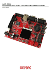
CLBs provide most of the logic that is implemented in an FPGA. A basic
diagram of the CLB is shown in Figure 2.1, taken from [1]. The three function
generators shown within each CLB allow it to implement certain functions of up to nine
variables. Each CLB also contains two storage elements, which can store function
generator outputs and can be configured as either flip-flops or latches. Adding to the
versatility of the CLB, the storage elements and the function generators can be configured
to be independent of each other. For example, the flip-flops can be used to store
(register) signals from outside the CLB where they reside. Also, the outputs of the
function generators need not pass through the flip-flops on the same CLB. Each CLB has
thirteen inputs and four outputs providing access to/from the function generators/storage
elements. The inputs and outputs of the CLBs are interconnected through the
programmable routing fabric. The different elements within the CLB are covered in the
following sub-sections.
2.2.1.1 Function Generators
Function generators provide the core logic implementation capabilities of a CLB.
Three function generators are provided, their outputs are labeled F’, G’, and H’ as shown
in Figure 2.1. All three of these function generators are implemented as look up tables
(LUTs).
4
F’ and G’ are the “primary” function generators. They are both provided with
four independent inputs and can implement any arbitrarily defined Boolean function of
up to four variables. H’ is the “secondary” function generator and is provided with three
inputs. Of these three inputs, one (H1) comes from outside the CLB, and the second can
come either from G’ or H0, and the third can come either from F’ or H2 (H0, H1, and H2
come from outside the CLB).
The outputs of the function generators can exit the CLB on two outputs, X and Y.
Only F’ or H’ can be connected to X; and only G’ or H’ can be connected to Y.
Additionally, the outputs of F’, G’, or H’ can be used as inputs to either of the two
storage elements whose outputs connect to the routing fabric (XQ and YQ).
Figure 2.1 - Simplified block diagram of the XC4000 Series CLB (RAM and carry
logic functions not shown) [1].
Given the attributes of the three function generators and their connectivity with
each other and the rest of the CLB, they can be used to implement any of the following:
5
1. Any function of up to four variables with a second function of up to four
unrelated variables and a third function of up to three unrelated variables.
2. Any single function of up to five variables.
3. Any function of four variables together with some functions of six variables.
4. Some functions of up to nine variables.
2.2.1.2 Storage Elements
The two flip-flops provided in the CLB allow the storage of two signals. These
signals can come from internal signals or from outside the CLB. The outputs of the flipflops can be connected to the routing fabric as well. The flip-flops can be configured as
either D flip-flops or latches. As D flip-flops they can be either falling or rising edgetriggered, and have a common clock (K) and clock enable (EC) inputs. When they are
configured as latches they also have the common clock and clock enable inputs.
2.2.1.3 Function Generators as RAM
Each CLB can be configured to use the LUTs in F’ and G’ as an array of
read/write memory cells. There are several RAM (Random Access Memory) modes in
which each CLB can operate: level-sensitive, edge-triggered, and dual-port edgetriggered. Given these modes a CLB can be implemented as a 16×2, 32×1 or 16×1 bit
RAM array.
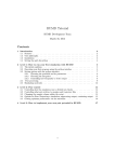
2.2.2 The Input/Output Block
The interface between the actual package pins and the internal logic of the FPGA
are provided through programmable input/output blocks (IOBs). Each IOB is connected
to one physical pin and can provide control of the pin for input, output, or bi-directional
signals. For each CLB there exists two IOBs. Figure 2.2 provides a simplified block
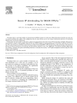
diagram of the IOB found in the XC4000E and Figure 2.3 shows the IOB for the
XC4000X. The IOB of the XC4000X contains special logic, that is not provided in the
XC4000E IOB, and these differences are shaded in Figure 2.3.
6
There are two paths that an external signal can traverse through the IOB to gain
entrance into the interconnection fabric in the FPGA; these are labeled I1 and I2 in both
Figure 2.2 and Figure 2.3. Either of these paths may contain a direct signal or a
registered signal, which passes through a register that can be configured as an edgetriggered D flip-flop or a level-sensitive latch. The XC4000X IOB also contains an extra
latch on the input. This latch is clocked by the output clock and allows for the very fast
capture of input data, which is then synchronized to the internal clock by passing through
the IOB flip-flop/latch.
Figure 2.2 - Simplified block diagram of the XC4000E IOB [1].
Signals that are output from the FPGA can be passed directly through the IOB to
the pad or registered into an edge-triggered flip-flop. Output signals can also be inverted
before they reach the pad.
Included in the XC4000X IOB is an additional multiplexer, which can be
configured not only as a multiplexer but also a 2-input function generator. This function
generator can implement a pass-gate, AND-gate, OR-gate, or XOR-gate with 0, 1, or 2
inverted inputs. When configured as a MUX, it allows two output signals to time-share
7
the same output pad, which can effectively double the number of device outputs without
expanding the physical package size.
2.2.3 Programmable Interconnect
All of the internal connections within the FPGA are composed of metal segments
with programmable switching points and switching matrices to implement the desired
connection of signals within the device. There are three basic classes of interconnect
available: CLB routing, IOB routing, and global routing. We will not discuss global
routing in this overview; the reader is referred to [1] for information on global routing.
Figure 2.3 - Simplified block diagram of the XC4000X IOB (shaded areas indicate
differences from XC4000E) [1].
2.2.3.1 CLB Routing
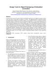
The CLBs are arranged in a grid array with the IOBs surrounding the grid. An
example layout is shown in Figure 2.4. The programmable interconnect is located
between CLBs and between the grid and the IOBs.
Each CLB has a myriad of interconnect resources to which it can connect its
outputs. A diagram representing these resources is shown in Figure 2.5. The five
8
interconnect types are single-length lines, double-length lines, quad and octal lines
(XC4000X only), and longlines that are distinguished by the relative length of their
segments. Table 2.1 shows how much of each interconnect type is accessible to a single
CLB. CLB inputs and outputs are distributed on all four sides of the CLB and in general
are symmetrical and regular. This makes the device well suited to placement and routing
algorithms. An additional feature is that inputs, outputs, and function generators can
effectively swap positions within a CLB, which can help in avoiding routing congestion.
CLBs
IOBs
Figure 2.4- Example layout of an FPGA with 16 CLBs [7].
9
Figure 2.5 - High-level routing diagram of the XC4000 Series CLB (shaded arrows
indicate XC4000X only) [1].
Table 2.1 - Routing per CLB in XC4000 Series devices [1].
XC4000E
XC4000X
Vertical Horizontal Vertical Horizontal
Singles
8
8
8
8
Doubles
4
4
4
4
Quads
0
0
12
12
Longlines
6
6
10
6
Direct Connects
0
0
2
2
Globals
4
0
8
0
Carry Logic
2
0
1
0
Toal
24
18
45
32
The single and double length lines intersect at Programmable Switch Matrices
(PSMs), shown in Figure 2.6. Each of these matrices consist of programmable pass
transistors, which allow the signals to be routed from one line to selected other lines of
the same type within the matrix.
Associated with each CLB are 16 single-length lines (8 vertical and 8 horizontal).
These lines offer the most flexibility and provide fast routing capability between adjacent
CLBs. They connect with PSMs located at every intersection of the rows and columns of
the CLB interconnect, this is shown in Figure 2.7. Signals on single-length lines are
10
delayed every time they go through a PSM, so they are generally not efficient for routing
signals for long distances. They are usually used to connect signals within a localized
area and provide branching for output signals with a fan-out (of greater than one).
Double-length lines are twice as long as single-length lines and they run past two
CLBs before entering a PSM, as shown below in Figure 2.7. These lines are grouped into
pairs with the PSMs staggered so that each line goes through a PSM at every other row or
column. There are four double-length lines associated with each CLB providing faster
routing over intermediate distances, while still retaining reasonable routing flexibility.
Associated with each CLB row and column in the XC4000X series devices are 24
(12 vertical and 12 horizontal) quad lines, which are four times as long as single-length
lines. These lines pass through buffered switch matrices and run past four CLBs before
doing so.
Each buffered switch matrix consists of one buffer and six pass transistors and
resembles a PSM, but only switches signals routed on quad lines. The matrix accepts up
to two independent inputs and provides up to two independent outputs. However, only
one of the independent inputs can be buffered. The Xilinx place and route software can
automatically decide whether or not a line should be buffered, given the timing
requirements of the signal. Buffered switch matrices make the quad lines very fast and in
fact quad lines are the fastest resource for routing heavily loaded signals long distances
across the FPGA.
Figure 2.6 - Programmable Switch Matrix (PSM) [1].
11
Longlines run the entire length or width of the CLB array and are used for high
fan-out, time-critical nets, or nets that span long distances. Two longlines per CLB can
be driven by 3-state drivers or open-drain drivers allowing them to implement
unidirectional buses, bi-directional buses, wide multiplexers, or wired-AND functions.
Each longline in the in the XC4000E series device has a programmable switch at
its center. In addition, each longline driven by an open-drain driver in the XC4000X
series device also has a programmable switch at its center. This programmable switch
can separate the longline into two independent lines, each spanning half the length or
width of the CLB array.
Every longline in the XC4000X series devices that is not driven by an open-drain
driver has a buffered programmable switch at the ¼, ½, and ¾ points of the CLB array.
This buffering keeps the performance of longlines from deteriorating with larger CLB
array sizes. If the programmable switch splits the longline, then each of the resulting
partial longlines are independent of each other.
In the XC4000X series device, quad lines are preferred over longlines when
implementing time-critical nets. The quad lines are faster for high fan-out nets due to the
buffered switch matrices that they pass through.
Figure 2.7 - Single- and double-length lines, with Programmable Switch
Matrices (PSMs) [1].
12
There are two direct connections between adjacent CLBs in the XC4000X
devices. These signals experience minimal interconnect delay and use no general routing
resources. This direct interconnect is also available between CLBs and adjacent IOBs as
shown in Figure 2.8.
2.2.3.2 I/O Routing (VersaRing)
The XC4000 Series devices also include extra routing around the IOB ring, which
is called a VersaRing and facilitates pin swapping and re-design without affecting board
layout. There are eight double-length lines spanning four IOBs (two CLBs), and four
longlines. Also included are global long lines and wide edge decoders, which are not
discussed here. For information on global long lines and wide edge decoders, the reader
is referred to [1]. The XC4000X has eight additional octal lines. A high level view of
the VersaRing is given in Figure 2.9.
Figure 2.8 - XC4000X direct interconnect [1].
In-between the XC4000X CLB array and the VersaRing there are eight
interconnection tracks (called Octals) that can be broken every eight CLBs by a
programmable buffer that can also function as a splitter switch. The buffers are staggered
so that each line goes through one every eight CLBs around the device edge.
When the octal lines bend around the corners of the device, the lines cross at the
corner so that the segment most recently buffered has the farthest distance to go until it is
13
buffered again. A diagram showing the bending of octals around corners is given in
Figure 2.10. IOB inputs and outputs connect to the octal lines via single-length lines,
which can also be used to communicate between the octals and double-length, quads and
longlines within the CLB array.
WED = Wide Edge Decoder (dark shaded areas indicate XC4000X only)
Figure 2.9 - High-level routing diagram of the XC4000 Series VersaRing (left edge) [1]
2.2.4 Power Distribution
The power distribution in the Xilinx XC4000 Series part is achieved through a
grid, in order to provide high noise immunity and isolation between logic and I/O. A
dedicated Vcc and Ground ring surrounds the logic array providing power to the I/O
drivers, while an independent matrix of Vcc and Ground lines provide power to the
interior logic of the device. A diagram showing this distribution method is shown in
Figure 2.11.
14
Figure 2.10 - XC4000X octal I/O routing [1].
Figure 2.11 - XC4000 Series power distribution [1].
15
CHAPTER III
BACKGROUND AND RELATED WORK
3.1 Basic Concepts of Power Consumption
This material is summarized from [7], which was developed under the same
research contract that supported the work of this thesis.
In order to predict the power consumption in a CMOS device, three types of
current flow need to be considered: leakage current, switching transient current, and load
capacitance charging current. The leakage current is related to the imperfection of field
effect transistors (FETs) that are used in CMOS devices. This type of current flow in
CMOS technology is very small and usually ignored when evaluating power
consumption.
CMOS gates consist of pairs of complimentary MOSFETs (metal-oxide
semiconductor field effect transistors). The switching transient current within CMOS
gates is caused by a brief short circuit that can occur when the state of the complimentary
gates change from on-to-off and off-to-on. This short circuit occurs when the
complimentary MOSFETs are concurrently “on” for a brief transient period of time. The
power loss due to switching transient current is dependent on the switching frequency of
the gate and is more considerable than leakage current.
The final type of current flow is load capacitance charging current. This is the
current flow that is required to charge the capacitance that is associated with a transistor
gate, and occurs when the state of a gate changes. This is the dominant type of power
consumption in CMOS devices, and is the only component of power consumption
considered in the remainder of this thesis.
3.1.1 Capacitance Charging Power Consumption
Two assumptions about CMOS transistors must be made in order to derive the
power consumption associated with capacitance charging. First, there is a non-zero
resistance in the electrical connection to the gate of each transistor. Second, the rate of
the switching of the transistor must be sufficiently slow for the capacitance to completely
16
charge or discharge. Figure 3.1 shows an equivalent model for the switching of a
transistor. The source voltage is V, the resistance in the connection to the gate is R, and
the capacitance of the gate is C.
Let τ represent the time that the switch remains at V before moving to ground.
Then, according to the derivations given in [7], the average power dissipated through the
transistor is (assuming that τ ≥ 4RC):
Pavg =
1
CV 2
2τ
.
(3.1)
Provided that there is non-zero resistance and the transistor fully changes state,
then all of the energy stored in the capacitor (C) is dissipated through the resistor during
the time interval τ. However, the amount of power dissipated when the transistor
changes state is dependent only on the amount of capacitance related to the gate (i.e., it is
independent of the value R). If the value of τ is decreased, indicating that the transistor is
changing states more frequently, then the power consumption will increase. This
indicates that the faster that a CMOS circuit runs, the greater the power consumption
related to the circuits operation.
V
t=0
R
C
Figure 3.1 - Equivalent gate model for a CMOS transistor [7].
3.2 Basic Concepts of Power Modeling
3.2.1 Time-Domain Techniques
Because the primary source of power consumption in CMOS ICs is due to the
current that is required to charge the capacitance associated with each transistor during
state transitions, the time-domain representation of all signals is therefore sufficient to
17
predict power consumption. This approach requires the simulation of time-domain data
signals throughout the device over the entire interval corresponding to the input data
stream [7].
For example, consider the logic function y = x1 x 2 x3 whose transistor level
implementation is shown in Figure 3.2. The input signals to the logical gates correspond
to the voltage levels for the gates of the transistors. In the time-domain approach, this
function requires that the voltages associated with each transistor be modeled, which is
illustrated in Figure 3.3.
x1
x2
x3
y
x1
y
x2
x3
Figure 3.2 – Illustration of a CMOS implementation for the Boolean function
y = x1 x 2 x3 [7] .
Figure 3.3 – Illustration of time-domain modeling of CMOS circuit signals [7].
After the voltage signals for each transistor being modeled are known, the average
power is computed for each gate g based on the number of transitions (Ng) the gate
18
experiences over the time interval T. Average power consumed by the gate g is then
given by :
1
CV 2 N g
2T
.
(3.2)
Therefore average power consumed by all gates in a device is given by:
Ng
1
CV 2 ∑
2
T
g∈all gates
.
(3.3)
In addition to this, the activity of the signal at gate g, relative to the gate frequency f, is
given by
( )
Ng
T
f
and will be denoted as Ag. Therefore the value of Ag is normalized
between zero and one. A value of 0.25 corresponds to a signal that transitions every
fourth clock cycle, on average, and a value of unity indicates that the signal transitions at
every clock cycle. Calculating Ag is straightforward when the time-domain signals
driving each gate g are known. The problem is that the determination of the exact timedomain signals is computationally expensive for the number of signals present in a
realistic design.
A power simulator called PET (Power Evaluation Tool) has been developed at the
University of California, Irvine that uses time-domain power modeling techniques [12].
This simulator models IC circuits developed using basic cell techniques. By estimating
power for each basic cell in a manner similar to estimating power for transistor gates, the
simulator can sum the power estimates for all cells to derive power consumption for the
entire device. This method of power estimation requires that the device be simulated and
that the simulator is given characteristic data about every type of cell used in the device.
This simulator is presented in [12] and is also used in order to estimate the power
consumption of a low-power divider developed in [6].
3.2.2 Probabilistic Techniques
Under the same contract as this thesis work, a probabilistic simulator has been
implemented and is covered in detail in [7]. A discussion of the current work being done
on this simulator is given in Section 3.2.2.1. Probabilistic techniques were used in order
19
to obtain acceptable results within a reasonable amount of computation time. The basic
notion behind this approach is to distill important probability-domain information from
the time-domain input. The probability-domain information can then be used in place of
the actual time-domain signal values in estimating average power and thereby removing
the dimension of time from the calculations, which reduces the complexity of the power
calculations considerably [7].
Two probabilistic parameters: signal probability and signal activity, are used in
[7]. The signal probability, denoted as p(s) for signal s, represents the percentage of time
that a signal has a logical value of one, while the signal activity, denoted as A(s) for the
signal s, is a normalized fraction of the signal’s activity divided by the device’s clock
frequency. The activity of a signal refers to the amount of times the signal changes state
from on-to-off and off-to-on during the period of interest. Illustrations of signal value
probability and signal activity measures are given in Figures 3.4 and 3.5, respectively.
p(clock) = 0.50
p(x2 ) = 0.29
p( x1) = 0.88
p(x3) = 0.69
Figure 3.4 – Illustration of signal probability measures associated with various timedomain signal data [7].
A(clock) = 1.0
A(x2 ) = 0.17
A(x1) = 0.10
A(x3) = 0.27
Figure 3.5– Illustration of signal activity measures associated with various time-domain
signal data [7].
In the paper by Parker and McCluskey [15] a symbolic method that relates
operations on Boolean data to corresponding operations on probabilistic data is
introduced. This allows a digital circuit simulation algorithm to operate on probabilistic
information; a detailed summary is given in [7]. Signal activities are “transformed” as
20
they pass through logic gates. This transformation is more complicated than probability
transformations. Signal probabilities must be known before the activity values are
calculated. These activity values are then used to model signal frequencies at the gates of
transistors and provide a straightforward way to estimate consumed power at the
transistor level. Then, the average power for each gate in the device can be calculated
and summed yielding the device’s power consumption. This method of estimating power
consumption is the basis of the power simulator presented in [7] and is briefly discussed
in Section 3.2.2.1. This power simulator estimates power at the CLB level of FPGAs
whereas the PET simulator [12] discussed in Section 3.2.1 simulates the device on the
basic cell level of ICs.
3.2.2.1 A Probabilistic Power Prediction Simulator
This section discusses the simulator that was developed in [7] and is currently
being calibrated. A brief discussion of how the simulator works and how it is being
calibrated is given here.
The simulator, which is implemented in Java, takes as input two files: (1) a
configuration file associated with an FPGA design and (2) a pin file that characterizes the
signal activities of the input data pins to the FPGA. The configuration file defines how
each CLB (configurable logic block) is programmed and defines signal connections
among the programmed CLBs. The configuration file is an ASCII file that is generated
using a Xilinx M1 Foundation Series utility called ncdread. The pin file is also an
ASCII file, but is generated directly by the user. It contains a simple listing of pins that
are used to input data into the configured FPGA circuit. For each pin number listed, the
probabilistic parameters of signal activity (As) and signal value (p(s)) are provided which
characterize the data signal for that pin.
Based on the two input files, the simulator propagates the probabilistic
information associated with the pins through a model of the FPGA configuration and
calculates the activity of every internal signal associated with the configuration. The
activity of an internal signal s, denoted As, is a value between zero and one and represents
21
the signal’s relative frequency with respect to the frequency of the system clock, f. Thus,
Asf gives the average frequency of signal s.
Computing the activities of the internal signals represents the bulk of
computations performed by the simulator. Given the probabilistic parameters for all
input signals of a configured CLB, the probabilistic parameters (including the activity) of
that CLB’s output signals are determined using a well-defined mathematical
transformation. Thus, the probabilistic information for the pin signals is transformed as it
passes through the configured logic defined by the configuration file. However, the
probabilistic parameters of some CLB inputs may not be initially known because they are
not directly connected to pin signals, but instead are connected to the output of another
CLB for which the output probabilistic parameters have not yet been computed (i.e., there
is a feedback loop). For this reason, the simulator applies an iterative approach to update
the values for unknown signal parameters. The iteration process continues until
convergence is reached, which means that the determined signal parameters are
consistent based on the mathematical transformation that relates input and output signal
parameter values, for every CLB.
The average power dissipation due to a signal s is modeled by ½ Cd(s)V2Asf, where
d(s) is the Manhattan distance the signal s spans across the array of CLBs, Cd(s) is the
equivalent capacitance seen by the signal s, and V is the voltage level of the FPGA
device. The overall power consumption of the configured device is the sum of the power
dissipated by all signals. For an N x N array of CLBs, signal distances can range from 0
to 2N. Therefore, the values of 2N + 1 equivalent capacitances must be known to
calculate the overall power consumption. Letting S denote the set of all internal signals
for a given configuration, the overall power consumption of the FPGA is given by:
1
Pavg = ∑ C d ( s )V 2 As f
s∈S 2
1
= V 2 f ∑ C d ( s ) As .
2
s∈S
(3.4)
The values of the activities (i.e., the As’s) are dependent upon the parameter
values of the pin signals defined in the pin file. Thus, although a given configuration file
22
defines the set S of internal signals present, the parameter values in the pin file impact the
activity values of these internal signals.
Let Si denote the set of signals of length i, i.e., Si = {s ∈ S | d(s) = i}. So, the set
of signals S can be partitioned into 2N + 1 subsets based on the length associated with
each signal. Using this partitioning, Eq. 3.4 can be expressed as follows:
1
Pavg = V 2 f
2
C 0 ∑ As + C1 ∑ As + L + C 2 N ∑ As .
s∈S
s∈S1
s∈S 2 N
0
(3.5)
To determine the values of the simulator’s capacitance parameters, actual power
consumption measurements are taken from an instrumented FPGA using different
configuration and pin input characteristics. Specifically, 2N + 1 distinct measurements
are made and equated to the above equation (Eq. 3.5) using the activity values (i.e., the
As’s) computed by the simulator. The resulting set of equations is then solved to
determine the 2N + 1 unknown capacitance parameter values. This is how the simulator
will be calibrated. For this study, the simulator will be calibrated for a Xilinx 4036
FPGA for which N = 36. The 73 required measurements are performed using six
different configurations (including various types of multipliers, adders, and FIR filters)
with approximately 12 pin files per configuration.
The simulator can then be evaluated by comparing computed average power
consumption from the simulator with corresponding actual measured power consumption
using configurations and pin files not used to calibrate the simulator.
3.3 A Low Power Divider
In [6], a low power divider was developed using power reduction techniques for
basic cell ICs. These methods are discussed in this section. All of the material in this
section is summarized from [6].
Although division is an infrequent operation compared to multiplication and
addition, it dissipates up to 1.4 times the amount of energy than floating-point addition.
This makes division a good candidate for evaluating low power design techniques.
The goal of the work was to reduce the energy consumption while maintaining the
current delay and keeping the increase in the area to a minimal amount. Because the
23
energy dissipation in a cell is proportional to the number of transitions, output load, and
to the square of the operating voltage, the author of [6] reduces the number of transitions,
reduces the load capacitance, and estimates the impact of using dual voltage. The
techniques used include switching off not-active blocks, retiming, using dual voltage, and
equalizing the paths to reduce glitches.
By switching off not-active blocks, parts of the circuit can be used only when
needed by the division algorithm thereby reducing the power dissipation of the block.
This is accomplished by forcing the input signals of the blocks to a constant value of one.
The next technique used was retiming the recurrence part of division. The
position of registers in a sequential system can affect energy dissipation, retiming
involves the repositioning of these registers without modifying their external behavior.
The energy that is dissipated within a cell is dependent on the square of the
voltage supply and reducing the operating voltage of the cells can produce a significant
decrease in the amount of energy dissipation. However, this technique can only be
applied to cells that are not in the critical paths of the circuit because the lower supply
voltage increases the delay through the cell.
Because of different delays throughout the device, the input signals to significant
parts of the circuit can arrive at different times. This has the effect of creating spurious
transitions within the sub-circuit until all signals have arrived. Spurious transitions add to
the energy dissipation in the sub-circuit because energy dissipation is proportional to the
number of transitions. To reduce the number of spurious transitions the author has
equalized the paths within the circuit in certain areas to reduce glitches that cause the
spurious transitions.
By using the techniques outlined in this section, the author of [6] was able to
decrease the power consumption of a radix-4 divider by 40 percent. However, a
fundamental problem with these techniques as applied to FPGAs is that the designer has
no control over how the CLBs in the FPGA are composed, placed, and how the signals
internal to the device are routed. In addition to this, dual voltage cannot be used in the
design of a circuit implemented in a FPGA due to the limitations of the current FPGA
technology.
24
3.4 The Practicality of Floating-Point Arithmetic on FPGAs
Many algorithms require floating-point operations running at the speed of tens or
hundreds of millions of calculations per second. These types of algorithms are candidates
for acceleration using custom computing machines (which includes reconfigurable
computing) [14]. However, in the past the implementation of floating-point operations
on reconfigurable platforms has not been considered seriously because the operations
require an excessive amount of area and do not map onto these devices well. With the
advent of VHDL (Very High Speed Integrated Circuit Hardware Description Language)
and more dense and faster FPGAs computing platforms, this technology may soon be
able to significantly speed up pure floating-point applications [5].
In the two articles discussed in this section, [14] and [5], the authors consider the
practicality of implementing floating-point arithmetic on FPGAs. They consider the size
of the FPGA implementations, speed, and the range of the numbers that can be
represented in the specified floating-point operations.
In [14], the authors consider eighteen- and sixteen-bit floating-point adders,
multipliers, and dividers synthesized for a Xilinx 4010 FPGA. The eighteen-bit format
uses a one-bit sign, a 7-bit exponent field (with a bias of 63), and a 10-bit mantissa
yielding a range of ±3.6875×10¹⁹ to ±1.626×10⁻¹⁹. The sixteen-bit format has a one-bit
sign, 6-bit exponent (with a bias of 31), and a 9-bit mantissa yielding a range of
±8.5815×10⁹ to ±6.985×10⁻¹⁰. The eighteen-bit floating-point format was used for a 2-D
FFT (2-Dimensional Fast Fourier Transform) and the sixteen-bit floating-point format
was used for a FIR filter. The authors conclude that custom formats derived for
individual applications are more appropriate than the IEEE standard formats [14].
In [5], the authors investigate the implementation of floating-point multiplication
and addition on Xilinx 4000 Series FPGAs. The system uses bit serial, booth recoding,
and digit serial algorithms for the integer multipliers, which are an integral part of
floating-point multiplication. The disadvantage of using a bit serial algorithm is that it
only resolves one bit of the product per cycle causing the system to take several cycles to
perform the multiplication. The digit serial algorithm resolves n bits of the product per
cycle, where n is the digit size [5].
25
The authors develop a floating-point multiplier and adder that is used in the
development of a multiply-and-accumulate circuit used for matrix multiplication. They
present a floating-point adder that fits in a Xilinx 4020E FPGA that performs at 40
MFLOPS (Millions of Floating-Point Operations Per Second). The floating-point
multiplier they developed can perform at a speed of 33 MFLOPS and can also fit into a
Xilinx 4020E. Therefore the multiply-and-accumulate unit developed can run at a peak
performance of 66 MFLOPS. (The authors do not state whether this unit can fit into a
single chip, but indicate that they used multiple FPGAs to implement the unit.) They
contend that with the newer Xilinx parts, that were not available when the study was
performed, they could potentially see a peak performance of 264 MFLOPS and a realized
performance of 195 MFLOPS on a system with four Xilinx 4062XL FPGAs. The
authors conclude that reconfigurable platforms will soon be able to offer a significant
speedup to pure floating-point computation [5].
26
CHAPTER IV
DESCRIPTION OF WORK PERFORMED
The work performed consists of familiarization with VHDL (Very High Speed
Integrated Circuit Hardware Description Language) [13], the Wild-One Reconfigurable
Computing Engine [11], Xilinx FPGAs [1], choosing a method of measuring power
consumption, and the implementation of two inner product co-processors (multiplyaccumulate and multiply-add) for both integer and floating point data. The target
architecture for the work (the Wild-One Reconfigurable Computing Engine from
Annapolis Microsystems) consists of a PCI card with two FPGAs, memory, support
hardware, and software.
The development environment provided by Annapolis includes source templates
and APIs. The APIs allow the designer to write C programs that can communicate with
and configure the on-board FPGAs. The system also has memory and a FIFO that can be
used for data storage.
After becoming familiar with VHDL and the Wild-One, several small designs
were implemented to gain experience with the system. The next accomplishment was to
design and implement a pipelined 12-bit integer multiplier, which is an integral part of
the inner product co-processors that were developed as a part of the work. A method to
measure the power consumed by the FPGAs on the Wild-One system (based on the
measurement of electrical current) was also chosen and evaluated, and this is discussed in
Chapter V. This chapter details the design of a 12-bit integer multiplier, a 16-bit floatingpoint multiplier, a 16-bit floating-point adder, integer and floating-point multiply-andaccumulate inner-product co-processors, and integer and floating-point multiply-and-add
inner-product co-processors.
4.1 An Array-Based Integer Multiplier
The multiplier implemented is a 12-bit array-based integer multiplier [2] and has
been implemented in several versions as a pipeline with one to eight stages. A basic
27
integer multiplier is a crucial part of a floating-point multiplier and needs to be well
defined.
The array-based multiplier, shown in Figure 4.1, was chosen because of the ease
with which it can be pipelined, improving the throughput of the multiplier. The arraybased design is easier to pipeline and has a greater throughput than an iterative
multiplication scheme because each level of computations only have to be performed
once to produce the final result.
The bulk of the multiplier is composed of Carry-Save Adders (CSAs) [2], which
are sets of vertically propagating adders. This allows the adders in a certain CSA to
depend only on the adders in the CSA above it in the path of signal propagation instead
of depending on adders located logically to the left and right. This not only simplifies the
adder units but also decreases the propagation delay of the signals through the adder
units.
b11A
b10A
b9A
b8A
b7A
b6A
b5A
b4A
b3A
b2A
b1A
b0A
CSA 0
carry
CSA 1
CSA 2
CSA 3
CSA 4
CSA 5
CSA 6
CSA 7
CSA 8
CSA 9
Propagate Adder
Figure 4.1 – An array-based multiplier.
28
sum
After the operands pass through the CSAs they also must pass through a
propagation adder [2]. This is due to the fact that each CSA produces a sum and a carry
value. The carry value must be used in order to produce a correct product. The structure
of the propagate adder is given in Figure 4.2.
The implemented multiplier has been tested for speed with different levels of
pipelining. The timing results are given in Table 4.1.
CSA 9
carry sum
Half Adder
carry sum
Full Adder
Full Adder
Full Adder
Full Adder
Full Adder
Full Adder
Full Adder
Full Adder
Full Adder
Full Adder
Full Adder
upper 13 bits of product
Figure 4.2 – A propagate adder.
As shown in Table 4.1 the multiplier can run at speeds of up to 39 MHz when
implemented in a Xilinx 4028ex FPGA and 50 MHz when implemented in a Xilinx
4036xla FPGA. This is probably due to the increased routing resources found in the
XC4000X series devices and the larger CLB array present in the 4036xla FPGA. The
Wild-One system can run at speeds of up to 50MHz, so testing beyond this speed was not
possible. One interesting aspect of these results is that in the 4036xla FPGA the speed of
the multiplier was limited to 29 MHz until 8 stages are used. We believe that a critical
29
path through the interconnection fabric was finally “broken” (i.e., with a registered stage)
when moving from seven to eight stages.
Table 4.1 – Timing results for the array multiplier.
# of stages Maximum Speed(Mhz)
4028ex
4036xla
1
14
28
2
19
25
3
21
N/A
4
22
27
5
29
28
6
39
28
7
22
29
8
33
50
4.2 Inner Product Co-processor Designs
The inner product co-processors implemented are floating-point and integer
versions of two co-processors: multiply-add and multiply-accumulate. High level
diagrams of the multiply-add and multiply-accumulate schemes are given in Figure 4.3
and Figure 4.4. The designs for these co-processors are detailed in the following
sections.
Input Buffer
Pipeline
Multiplier
Pipeline
Multiplier
Pipeline
Adder
Output Buffer
Figure 4.3 - Multiply-add scheme.
30
4.2.1 Floating-Point Co-processors
The major difference between the two co-processors is that one of them has an
accumulator instead of only an adder. The accumulator is an extension of the adder and
therefore both the adder and accumulator based designs consist of the multiplier and
adder which are detailed below.
Input Buffer
Pipeline
Multiplier
Pipeline
Adder
Output Buffer
Figure 4.4 - Multiply-accumulate scheme [9].
The floating point format chosen is a 16-bit floating point format supported by the
ADSP-2106x family of SHARC DSP processors produced by Analog Devices [8]. This
format uses an 11-bit mantissa, a 4-bit exponent, and a one-bit sign. The exponent is
represented in excess-7 notation. This format is shown in Figure 4.5 and has an accuracy
of ±1.5625×10⁻² to ±2.559375×10².
Short Word Floating Point Format
15 14
s
11 10
e3•••e0
0
1.m10•••m0
Figure 4.5 - SHARC DSP short word floating point format [8].
31
4.2.1.1 Floating-Point Multiplier
The floating-point multiplier is shown in Figure 4.6, which is adapted from [9].
The multiplier consists of sign logic, an excess-7 exponent adder, an array-based
multiplier, and normalization logic. The multiplier is designed to allow for differing
levels of pipelining.
Because the exponents are stored in excess-7 notation, the exponent adder must
add the two excess-7 numbers and then subtract seven from the sum; otherwise it would
produce an “excess-14” sum. If the normalization requires that the exponent be adjusted,
then the exponent will only have to be adjusted by increasing it by a value of one. When
this occurs, the excess-14 sum is decreased by a value of six instead of seven, which
effectively increases the final exponent sum by a value of one. The reasons for this are
discussed below.
In the excess-7 exponent encoding used by the SHARC DSP, a value of zero
indicates that the value of the floating-point number is exactly zero and an exponent
value of fifteen indicates that the value of the floating-point number is infinity. Because
of this, the floating-point multiplier, shown in Figure 4.6, must check the exponents for
these two cases and set the resulting exponent to the appropriate value. Additionally, if
underflow occurs in the exponent addition, then the resulting exponent needs to be set to
zero because the actual resulting exponent is below the range of values that are
representable. Accordingly, if overflow occurs in the exponent addition, then the
resulting exponent needs to be set equal to fifteen, which represents infinity, because the
actual resulting exponent is above the range of values that are representable.
The 12-bit array-based multiplier is the multiplier discussed in Section 4.1. The
multiplier produces a 24-bit product of which only 13 bits are needed to generate the
correct resulting mantissa. The product must be normalized before it is stored in the 16bit floating-point format used. The msb of the product indicates which bits are needed
for the resulting mantissa.
Both the multiplicand and the multiplier have the forms of 1.bbb...b with a width
of w. When these two values are multiplied together, the product has a width of 2w and
is of the form of either 01.bb...b or 10.bb...b. Example multiplications (with w = 4)
32
resulting in products with each of these forms are given in Figure 4.7. If the msb of the
product is 1 (Figure 4.7(a)), then the product must be shifted to the right one place
resulting in the exponent needing to be increased by a value of one. (This allows us to
use the msb of the product as the ‘exponent adjust select’ in Figure 4.7.) If the msb of the
product is 0 (Figure 4.7(b)), then the position msb - 1 will always have a value of one, in
which case no normalization or exponent adjustment is needed.
s 1 s2
e1
1.m1
e2
e1(0)
e2(0)
e1(1)
e2(1)
e1(2)
e2(2)
e1(3)
e2(3)
1.m2
excess-7 adder
1
12 bit Array-Based
Multiplier
exponent
adjust
select
upper 13 bits of product
0
0
If the msb = 1 take the
bits msb-1…msb-11
1
If the msb = 0 take the
bits msb-2…msb-11
1
10
11
unf
ovf
exponent
mantissa
If underflow = 1, set exponent = 0
If overflow = 1, set exponent = 15
(representing infinity)
If e1 or e2 = 0, set exponent = 0
If e1 or e2 = 15, set exponent = 15
1 bit
4 bits
sign
exponent
11 bits
mantissa
Figure 4.6 - 16-bit floating-point multiplier.
33
4.2.1.2 Floating-Point Adder
The floating-point adder chosen is a pipelined adder [9] and is shown in Figure
4.8. By using subtraction to compare the exponents, it can determine how much the
mantissa of the value with the smaller exponent needs to be adjusted in order to align the
mantissas, while at the same time determining which exponent will be used to compute
the exponent of the result. Because the exponent comparison determines the difference,
the fact that the exponents are stored in excess-7 notation is not relevant. A diagram
showing the comparison of the exponents is given in Figure 4.9. The method of selecting
the exponent to be used for the final result is by using multiplexers to select the exponent,
this is shown in Figure 4.10, and depends only on the sign of the difference obtained in
the comparison of the exponents.
The next task in floating-point addition is to align the mantissas so that the radix
point is lined up in the same position for the two mantissas. The phantom bit (which has
a value of one for non-zero operands) must be appended to the msb of each of the
mantissas before this alignment can occur. The alignment is shown in Figure 4.11. Only
one mantissa needs to be shifted and this is determined by the value of the sign of the
difference obtained in the exponent comparison. The difference obtained in the exponent
comparison determines how many places to the right the selected mantissa must be
shifted.
1.101
× 1.110
0000
1101
1101
1101
10.110110
1.001
× 1.011
1001
1001
0000
1001
01.100011
(a)
(b)
Figure 4.7 - Two possible normalization cases in floating point multiplication.
34
e1
e2
4
m1 m2
4
11
s1
11
Check for Absolute Zero and Infinity and Add Phantom Bit
12
12
Registers
Compare Exponents
by Subtraction
difference
4
pos./neg.
1
Registers
Choose Exponent
Align Mantissas
Registers
Add/Subtract
Mantissas
Registers
Normalize Mantissa and Adjust Exponent
4
exponent
11
mantissa
1
sign
Figure 4.8 - Pipelined floating-point adder [9].
35
s2
1
1
0e1
0e2 1
5
1
5
5
5-Bit Adder
4
3
2
1
1
0
If pos./neg. = 1, choose e2
Else choose e1.
pos./neg.
exponent difference
Figure 4.9- Comparing exponents by subtraction.
e2
pos./neg.
e1
4
4
1
1
0
4 - 2 by 1
Multiplexers
If pos./neg. = 1, choose e2
4
Else choose e1.
exponent
Figure 4.10 – Choosing of the exponent.
pos./neg.
1.m1
Right Shift Unit
difference
1.m2
sel
Right Shift Unit
~1.m1
~1.m2
Figure 4.11 - Align mantissas.
36
sel
The addition/subtraction of the mantissas is shown in Figure 4.12. If one of the
values is negative, it must be converted to 2’s complement in order to perform
subtraction. Additionally, if the resulting sum is negative, it must be converted back to
sign-magnitude form. If both of the values are negative, then regular addition can be
performed because the sign logic accounts for this case. Because addition will result in a
sum (at most) twice as big as the largest operand, an extra bit must be used in the
addition. Therefore, the addition requires a 13-bit adder because our operands are 12 bits
in size. Another adder is required to convert the sum back into sign-magnitude form (if
the sum is negative). The sign bit is used to determine the resulting sign of the sum value
and to determine if conversion from 2’s complement representation to sign-magnitude
representation is necessary.
Figure 4.12 - Add/Subtract mantissas.
37
The final step in floating point addition is to normalize the mantissa and adjust the
exponent, which is shown in Figure 4.13. There are three possible cases to deal with in
normalization:
1. If bit 12 of the sum has a value of one, then the mantissa is shifted one place
to the right and the exponent is incremented by a value of one. An example of
this is shown in Figure 4.14(b).
2. If bit 12 of the sum has a value of zero and bit 11 has a value of one, then the
mantissa is already normalized and no exponent adjustment is necessary. An
example of this is shown in Figure 4.14(a).
3. Otherwise, we do not know where the leftmost bit with a value of one occurs
in the sum. In the worst case it is the lsb, in which case we must shift the
mantissa eleven places to the left and decrement the exponent by a value of
eleven. An example of this is shown in Figure 4.14(c). The actual
implementation of this selects the bits from the mantissa being shifted and
does not actually shift the mantissa.
After the mantissa has been normalized and the exponent has been adjusted, we
have the final answer represented in the 16-bit floating-point format.
4.2.2 Integer Co-processors
The integer co-processors are composed of an integer multiplier and an integer
adder with the necessary control to perform multiply-add and multiply-accumulate
operations. The high level designs for these co-processors is presented in Section 4.2 and
is the same as for the floating-point co-processors. The data format chosen for the integer
co-processors is unsigned 16-bit integer. The data format has a range of 0 to 65535.
The multiplier is an expanded 16-bit version of the 12-bit array-based multiplier
presented in Section 4.1. The adder is a basic 16-bit carry-propagate adder similar to the
ones used for the adding and subtracting operations found within the floating point adder
discussed in Section 4.2.1.2.
38
Exponent (4 bits)
Mantissa (13 bits)
If Mantissa(12) = 1 then take bits 11 downto 1
and add one to the exponent.
Else if Mantissa(11) = 1 then take the bits 10 downto 0
and do nothing to the exponent.
Else take the bits 10 downto 0
and shift the bits to the left until the msb = 1
subtracting 1 from the exponent every time a shift occurs.
Then take the upper 11 bits.
Normalized Answer
(Exponent and Mantissa)
Figure 4.13 - Normalize mantissa and adjust exponent.
001.001
001.001
+ 000.010
+ 001.000
001.011
- 001.000
001.011
010.001
000.011
(a)
No normalization
needed.
(b)
Shift one place
to the right.
(c)
Shift left two
places.
Figure 4.14 - Examples of normalization.
39
CHAPTER V
RESULTS AND IMPLEMENTATION ISSUES
The proposal for this master’s thesis outlined five objectives for the master’s
thesis work to accomplish. These objectives are:
1. More fully understand power modeling techniques and past research in this
area.
2. Implement and compare the floating-point and integer inner product coprocessors.
3. Understand why inserting more stages does not always increase the maximum
speed of a pipelined circuit.
4. Understand the power consumption reduction seen by using more pipeline
staging registers.
5. Calibrate the power simulator developed previously in [7].
Each of these objectives and their outcome is discussed in this chapter along with
implementation issues encountered during the implementation of the inner product coprocessors.
5.1 Problems with Measuring Real Power Consumption
The first objective outlined in the proposal was to more fully understand power
modeling techniques and past research in this area. This objective goes along with the
last objective outlined in the proposal, which was to calibrate the power simulator
developed previously in [7]. While there was a literature review performed on past
research in this area we were not able to calibrate the power simulator. After some
investigation into how to calibrate the power simulator we realized that it was a more
monumental task than believed at first and was not a reasonable goal for the time allotted
to finish this work.
The main problem we ran into in trying to calibrate the simulator is with the
accurate measurement of real power consumption. We obtained an FPGA board for
which current for the entire FPGA board can be measured. However, after taking
40
measurements for long periods of time it was discovered that the values would drift
slowly up and down significantly. Because the power measurements taken initially may
not be accurate, the fourth objective (which was to understand the power consumption
reduction seen by using more pipeline staging registers) could not be accomplished. It
was not possible to perform real power measurement tests on differently staged pipelines
with the given apparatus.
5.2 Performance and Comparison of the Co-processors
The original intent was to pipeline the co-processors enough to get every coprocessor running at 50 MHz. However, due to a lack of time this was not accomplished.
Instead the co-processors were tested for speed and estimated power consumption using
the latest version of the power simulator.
The only implementation issue had to do with the multiply-and-add circuits.
These circuits required that four operands be fed into the two multipliers at the same
time. Because the memories on the Wild-One are only 32-bits wide and the operands are
16-bits in size, this required a scheme of clocking two operands into the circuit every
clock cycle and running the circuit at half of that clock speed. So effectively the circuits
produce answers at half of the rate the whole system is running. In both the integer and
floating-point versions of this circuit, answers intermittently come back wrong. Because
the circuits also produced correct answers for the same data as wrong answers, it is likely
that the multiplier and adders work correctly and that the intermittent failure has to do
with something on the system level. This may be due to a poor job of placing and routing
the circuits into the FPGAs by the Xilinx tools used. However, the exact cause for these
intermittent failures was not determined. It is suspected that this problem has to do with
the scheme of introducing a secondary clock signal, which clocks the multipliers and
adders at half the speed of the system clock. The Xilinx tools and/or FPGA may not be
able to effectively distribute this second clock signal.
The timing measurements, resource utilization, and estimated power consumption
for each co-processor is given in Table 5.1.
41
The integer co-processors are able to run faster than the floating-point coprocessors. This is a trade-off in that the integer co-processors have a different input
range (0 to 65535) than the floating-point co-processors (±1.5625×10⁻² to
±2.559375×10²). Another trade-off is that the integer co-processors also take more space
in the FPGA than their counterpart floating-point co-processors, which make a difference
in power consumption and how many of the co-processors could potentially be fit into
one chip.
In order to estimate power consumption of the co-processors, each co-processor
was run through the power simulator developed in [7] (discussed in Section 3.2.2.1) using
two different input data files. (The simulator did not converge for the integer multiplyaccumulate co-processor for some reason; it would eventually reach a point where it
would run for over 12 hours with no progress.) These files contain probabilities and
activity factors for each input signal into the circuit. One of the two files had random
probability and activity factors in it while the other one had the values increasing and
decreasing across the input signals, similar to a periodic waveform. While the
capacitance associated with each of the different 73 signal distances across the FPGA is
not known at this time, the simulator computes the activity values for each different
signal distance and returns these values. The equation, which is adapted from Eq. 3.5,
used for calculating estimated power is:
1∑ As + 2 ∑ As + ⋅ ⋅ ⋅ + 2 N ∑ As + (2 N + 1) ∑ As .
s∈S
s∈S 1
s∈S 2 N −1
s∈S 2 N
0
(5.1)
While this does not give an accurate power consumption estimate it gives some idea of
what the power consumption of the device will be assuming that the capacitance
associated with the signals in S0 is less than the capacitance associated with signals in S1
to S2N. Instead, this gives a weighted sum that can be used to estimate the power
consumption value the simulator will return for the design when it is calibrated. Figure
5.1 shows a comparison of activity values for each different signal length for the floatingpoint versions of the Multiply-Accumulate and Multiply-Add co-processors. The two
activity value sums for interconnection lengths 30 and 31 are caused by the feedback for
the accumulation part of the multiply-accumulate circuit. These two values alone make
42
up the difference of 60 between the two co-processors. From this result we can conclude
that non-regular signals (such as these) which go against the direction of data flow in the
circuit cause increased power consumption. This is because these signals have to be
routed long distances around a subset of CLBs in order to be input signals to this subset
of CLBs.
Table 5.1 – Speed, Resource Utilization, and Estimated Power Consumption of
the Co-processors.
Speed # of # of
# of
# of
Equivalent Estimated Power
Co-Processor
(MHz) CLBs Flip-Flops 3-Input LUTs 4-Input LUTs Gate Count Consumption
Integer Multiply-Accumalate
50 622
720
180
794
10076
N/A
Integer Multiply-Add
43 1013
1148
423
1421
16809
415
F.P. Multiply-Accumalate
38 437
414
154
742
8072
454
F.P. Multiply-Add
34 716
654
254
1082
11766
390
Multiply-Add vs. Multiply-Accumulate
Linearly Weighted Activity Values
70
Linearly Weighted Activity Values
60
50
40
30
20
10
46
44
42
40
38
36
34
32
30
28
26
24
22
20
18
16
14
12
10
8
6
4
2
0
0
Interconnection Length
Multiply and Add
Multiply and Accumulate
Figure 5.1 – Linearly weighted activity values for multiply-add and multiply-accumulate.
43
5.3 A Phenomenon Observed with Pipelining
The fourth objective of this thesis was to understand why inserting more stages
does not always increase the maximum speed of a pipelined circuit. Since the coprocessors were not pipelined with varying numbers of pipeline stages, this was not
investigated much at all. This phenomenon is observed with the array-based multiplier
discussed in Section 4.1.
The reason this is believed to happen is because the 4028ex FPGA has less CLBs
and routing resources than the 4036xla FPGA. This has caused the Xilinx tools to place
and route the design into the 4028ex in such a way that signal connections and/or CLBs
are placed so that one or more signals travel a long distance. In order for a given CLB to
run at a certain speed, all of the input signals to that CLB must originate within a certain
distance, given the type of interconnection that is used to route the signal, as to delay the
signal no more than the threshold of delay for running the CLB at the given speed. This
is what has happened with the multiplier implemented in the 4028ex part; either signals
or CLBs were routed in a poor fashion.
44
CHAPTER VI
CONCLUSIONS AND FURTHER RESEARCH
This study has demonstrated that inner-product co-processors for both integer and
floating-point data can fit into today’s FPGA technology and achieve a significant speed
and throughput. The results of this implementation shows that it is feasible and
beneficial under certain circumstances to implement floating-point and integer operations
in FPGAs (i.e., such as when a custom data format can be used, as with the SHARC DSP
which can convert back and forth between IEEE 32-Bit floating point and the SHARC
DSP 16-bit floating point formats).
This study did not calibrate the simulator of [7] nor evaluate the co-processors on
the basis of real power consumption. This is due to the problems encountered in
measuring real power consumption. This is an area that still needs to be further
researched and refined. The successful calibration of the probabilistic power simulator
will be of a major benefit to the reconfigurable and power-aware communities. In
addition to this, the simulator needs to be expanded to handle different brands and models
of FPGAs.
The estimation of power consumption in Chapter V has shown that the data flow
within a design has an impact on power consumption. When the data flow is non-regular,
as in the accumulation part of the multiply-accumulate co-processor, the power
consumption will increase if the design cannot be efficiently placed and routed into the
FPGA.
Once the simulator has been calibrated and a method of measuring real power
accurately has been achieved, then a study into the effects of pipelining on power
consumption needs to be performed. The general expectation is that more pipelining will
cause more power consumption. A sweet spot should exist between the trade-offs of
throughput and power consumption for each different application. This study could also
attempt to identify methodologies for exploiting the power consumption characteristics of
FPGAs. The overview of the Xilinx XC4000 Series FPGA found in Chapter II provides
45
a good foundation for understanding the characteristics of these FPGAs which may
impact power consumption.
46
REFERENCES
[1]
Xilinx XC4000E and XC4000X Series Field Programmable Gate Arrays, Product
Specification, Xilinx Inc., v1.5, [online]
http://www.xilinx.com/partinfo/databook.htm#xc4000, 1999.
[2]
J.L. Hennessy, Computer Architecture: A Quantitative Approach, Second Edition,
Morgan Kaufmann Publishers Inc., San Francisco, California, 1996.
[3]
K. Roy and S. Prasad, “Circuit Activity Based Logic Synthesis for Low Power
Reliable Operations,” IEEE Trans. Very Large Scale Integration (VLSI) Systems,
Vol. 1, No. 4, December 1993, pp. 503-513.
[4]
T.L. Chou, K. Roy and S. Prasad, “Estimation of Circuit Activity Considering
Signal Correlations and Simultaneous Switching,” Proc. IEEE International
Conference on Computer-Aided Design, pp. 300-303, Nov. 1994.
[5]
W.B. Ligon III, et al., “A Re-evaluation of the Practicality of Floating-Point
Operations on FPGAs,” IEEE Symposium on FPGAs for Custom Computing
Machines, April 1998, pp 206-215.
[6]
A. Nannarelli and T. Lang, “Low-Power Divider,” IEEE Trans. Computers, Vol.
48, No. 1, January 1999, pp. 2-14.
[7]
T. Osmulski, Implementation and Evaluation of a Power Prediction Model for
Field Programmable Gate Array, Master’s Thesis, Computer Science, Texas
Tech University, 1998.
[8]
ADSP-2106x User's Manual, Second Edition, Analog Devices, [online]
http://www.analog.com/publications/documentation/ADSP_2106x_SHARC_User
s_Manual/books.html, 1996.
[9]
M.M. Mano, Computer System Architecture, Third Edition, Prentice Hall Inc.,
Englewood Cliffs, New Jersey, 1993.
[10]
N. Gupta, Reconfigurable Computing for Space-Time Adaptive Processing,
Master’s Thesis, Computer Science, Texas Tech University, 1998.
[11]
Wild-One Reconfigurable Computing Engines: Manual, Revision 3.2, Annapolis
Micro Systems Inc., Annapolis, MD, 1998.
[12]
A. Nannarelli, “Power Evaluation Tool: Modeling and Implementation,” Proc.
1996 Compass User’s Group Conference, April 1996.
47
[13]
K. Skahill, VHDL for Programmable Logic, Addison-Wesley, Reading,
Massachussetts, 1996.
[14]
N. Shirazi, A. Walters and P. Athanas, “Quantitative Analysis of Floating Point
Arithmetic on FPGA Based Custom Computing Machines,” Proc. IEEE
Symposium on FPGAs for Custom Computing Machines, April 1995.
[15]
K.P. Parker and E.J. McCluskey, “Probabilistic Treatment of General
Combinatorial Networks,” IEEE Trans. Computers, vol. C-24, pp. 668-670, June
1975.
48