Download Joule‐Thomson Cold Finger Design and Analysis

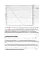
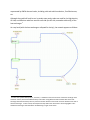
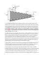
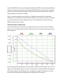
 Joule‐Thomson Cold Finger Design and Analysis A Joule‐Thomson (JT) device achieves cooling by throttling a real gas from a high pressure to a low pressure. A perfect gas exhibits no JT effect: the isenthalpic expansion of a perfect gas is also an isothermal process. Therefore, not all expansions result in a drop in temperature: in some cases, the temperature can rise. Gases such as nitrogen, argon, krypton, and helium exhibit a temperature drop with expansion, and can therefore be used for cooling applications. Furthermore, each of these gases has a different starting pressure for achieving the maximum cooling effect. For nitrogen, for example, the JT cooling effect peaks when starting near 5000 psia. JT devices can be used in stages, and in combination with other cryocooling techniques. They are not very efficient thermodynamically, so they tend to be used in applications where small, compact (and motionless) cold fingers are required, or in short‐lived applications in which a transient (blow‐down) source is sufficient, such as cooling IR sensors in a missile or probe. A closed‐loop cycle involving a JT throttle is called a Linde‐Hampson cooler, which is basically a JT cold finger with continuous high pressure gas provided by a compressor instead of a bottle. The hot gas at the outlet of the compressor is cooled using the environment as a sink. A simple venture or orifice can be used as a throttling device, but often a more complex option is employed to avoid the need for very small openings (which can clog due to the freezing of contaminant gases). One option is a nozzle tube or orifice tube. Another is a labyrinth “seal”1 … effectively a series of larger‐aperture orifices in series. The performance of a JT device can be significantly enhanced by precooling the high pressure (HP) fluid using the colder exhaust fluid from the low pressure (LP) side of the throttle. A Giauque‐Hampson counter‐flow finned‐pipe heat exchanger (also known as a precooler or recuperator) is a common option. The purpose of this document, and the associated thermal/fluid models, is to illustrate the application of SINDA/FLUINT, Sinaps©, and Thermal Desktop©/FloCAD© to •
•
•
JT cryostat analysis Modeling of gas labyrinth seals (even though they purposely leak in this application) Modeling of heat exchangers in general, at both the system and detailed levels 1
www.gpcvalves.com/downloads/jt.pdf
Labyrinth “flow spoilers” is the term used by GPC, but since many applications of stepped labyrinths are to reduce flow in rotating turbomachinery, the term “seal” or “throttle” will be used here. A preliminary design will be developed first. At this top level, the throttle will be considered as a simple (single) orifice, and the heat exchanger will be treated at a system‐level using effectiveness/NTU methods. This preliminary model will be prepared using Sinaps. Subsequently, a more detailed model will be developed in which the labyrinth seal will be designed and modeled in more detail. Also, the heat exchanger will be modeled in more detail in this second round, demonstrating application of compact heat exchanger techniques. This detailed model will also be prepared using Sinaps, although a Thermal Desktop/FloCAD representation of the final design will also be presented. Design Requirements and Constraints The unit will be required to cool a 1W load at 80K. The load has a thermal mass of 30 gm (0.066 lbm) and a specific heat (Cp) of 300 J/kg‐K, and is connected to the cold finger via a linear conductance of 1 W/K. Nitrogen at 300K and 5000 psia (35 MPa) is available, and may be exhausted to ambient pressure. Minimal nitrogen consumption is desired. A compact single‐stage cryostat is desired, with an overall length of no more than about 4cm (approx 1.5”) and diameter no greater than about 1.5cm (approx. ½”). The details of the source of nitrogen have been purposely omitted: it might be a very large bottle, and it might be the compressor and gas cooler in a Linde‐Hampson cycle. Either way, the implication of assuming an infinite source is that only a steady‐state analysis need be used. This has tremendous impact on the resulting design and analysis. Therefore, it should be mentioned that blow‐down JT systems can and have been analyzed using SINDA/FLUINT, including cool‐
down transients and even automated optimization of components to achieve both rapid cool‐
down as well as sustained operation. In such a blow‐down system, a reservoir is usually available downstream of the throttle to store any liquid that is generated, and some means is provided for preferentially exhausting only vapor from that reservoir … or at least discouraging loss of low‐enthalpy liquid. For a steady system, a small amount of liquid (e.g., high quality two‐
phase fluid) may enter the low pressure side of the precooler. Many details are obviated by assuming that this device operates at steady‐state, since the purpose of this model is to demonstrate other modeling techniques (e.g., laby seals and heat exchangers). However, since many JT applications are indeed blow‐down systems in which cool‐
down characteristics and liquid production and consumption are important, the FloCAD‐based model includes a demonstration of such transient capabilities. The high pressure line is 0.013”(0.33mm) ID, and is made of 70‐30 copper‐nickel alloy. Soldered copper fins are available, but with the smallest fin thickness available being 0.0025” (0.064mm). Preliminary Design For preliminary design purposes, the throttle will be treated as an effective orifice, and a toothed labyrinthine passage or “laby seal” will be sized later to provide the same throttling action once the JT flow rate and throttle inlet conditions are known. Similarly, the heat exchanger will largely be sized based on ε‐NTU (system‐level, inlet/outlet) methods, and a more detailed model will be used once the basic design is known. However, the overall UA of the heat exchanger can only be estimated at this preliminary stage of design. The overall UA will be a strong function not only of the geometry of the heat exchanger (e.g., axial fin spacing and OD of the annular fins), and of the throttle (which largely determines the flow rate and which cannot be sized independently of the heat exchanger’s performance). But the overall UA will also be a function of the local temperatures and pressures, which vary greatly on both sides of the heat exchanger. Furthermore, unlike many heat exchanger sizing exercises, the temperature on the cold (low pressure, or “LP”) side is not known ahead of time: it is a function of the throttle and of the design of the heat exchanger itself. In other words, this is a strongly coupled problem. Also the possibility of two‐phase fluid entering the LP side of the heat exchanger further complicates the design. A detailed model could easily encompass all of these details, but it would be slower to solve, and clearly many iterations will be required to arrive at a satisfactory design. Therefore, a highly approximate model will first be used to narrow the range of possibilities, and to arrive at a starting point for the more detailed design. As will be seen, this top‐level model is a cross between a spreadsheet analysis and a four point cycle (thermodynamic state) analysis. The term “overall UA” is not to be confused with the FLUINT convection tie “UA,” which is the local conductance of that tie. Unless it is used as a segment tie, the UA of a tie is actually the “hA” in heat exchanger terminology: the local film coefficient times the local heat transfer area that is the basis of that coefficient. In other words, the “overall UA” of the heat exchanger can be calculated if all of the local tie UA’s are known … along with other factors such as fin efficiency, constriction resistances, fouling resistances, etc. The Sinaps model used for the preliminary design is available for inspection (or for use as a starting point): sizing.smdl. Therefore, no attempt will be made to document the model in detail. Rather, this write‐up seeks to provide an explanation of the approach used, and should be viewed as a companion to the data available in the model. Basic familiarity with both Sinaps and SINDA/FLUINT is assumed. Modeling the Load Actually, the specification of “1W at 80K” would over‐specify any single steady‐state analysis: either the load can be modeled as a boundary node at 80K and the design adjusted such that 1W is extracted from it, or the load can be modeled as a diffusion or arithmetic node with a source of 1W, and then the design is adjusted such that the node is maintained at 80K. The latter mode (given Q, find T) was used in this analysis, but provisions for the opposite mode (given T, find Q) are available as well.2 The load was modeled as a single diffusion node, load.1, and it was tied to the downstream of the throttle using an HTU tie with UA=1. Some of the registers used to define the load and boundary conditions are shown below: Modeling and Sizing the Throttle The throttle is initially modeled as a simple orifice, since the adiabatic expansion in such a device will be similar to most mechanisms which cause a pressure drop. An orifice essentially has only one degree of freedom: the throat size or aperture. This simplified treatment facilitates answering the central preliminary design question: What minimum flow rate achieves 1W of cooling at 80K? The orifice model will be replaced by a labyrinth seal model with more specific dimensions at a later stage, but the primary goal of that more complex design will be to achieve the same mass flow rate as did the orifice (albeit with a larger minimum flow area for reduced risk of clogging). Unfortunately, the flow rate cannot be determined separately from the heat exchanger design: they must be sized simultaneously. The strongest cross‐influence is the temperature of the precooled fluid at the outlet of the throttling device, but a secondary influence is the pressure drop of the heat exchanger. If a large heat exchanger is needed to accomplish the design, then 2
The diffusion node can be “held” as a temporary boundary node via a call to HTRNOD in OPERATIONS. This call is optionally invoked via use of the LoadMode register. Of course, the node type could also be simply changed in Sinaps “permanently.” a nonnegligible pressure drop in the heat exchanger will mean a lower pressure gradient available to the throttle: both a decreased upstream pressure (due to flow losses in the HP side of the heat exchanger), and an increased downstream pressure (due to flow losses in the LP side). Some amount of iteration will therefore be needed. In fact, this would be a good problem for the SINDA/FLUINT Solver (design optimization module), which could automatically achieve a honed preliminary design, presuming that the user sufficiently “explains” the problem in terms of objectives and constraints. However, because this example problem is already lengthy, and because the preliminary model is highly simplified, a simpler but cruder method will be used: a couple of parametric sweeps which are exercised a few times each in order to close the design iteration. Assuming that an approximate heat exchanger design has been established (as explained in the next section), a simple parametric sweep of orifice hole sizes is made, plotting both the temperature of the load (at 1W dissipation), and the estimated NTU of the heat exchanger (register NTUeff). The required design will be that which achieves the 80K requirement, and which doesn’t require more than the estimated heat exchanger performance. As seen in the plot below, the minimum orifice size is 0.14 times the flow area of the HP line (corresponding to a mass flow rate of about 0.86 gm/s or 6.8 lbm/hr) since that is the size that yields an 80K load. This throttle flow area fraction is expressed as the register Oratio, noting that the ID of the HP line is contained in the register IDhp: The plot below was made using an input (assumed) NTU of 5 (effectiveness of 0.8333 for counterflow), and at the design point (Oratio=0.14) the estimated performance of the heat exchanger is about NTUeff=4.9. This agreement verifies that the predicted performance of the heat exchanger (NTUeff) is about the same as that required (NTU): the orifice sizing can therefore be trusted. If the heat exchanger design was enlarged or reduced, then the above sizing would need to be repeated using the new baseline heat exchanger design. Fortunately, few such iterations are required to close on a design. The sudden jump in the NTUeff at an Oratio of about 0.08 corresponds to the transition from laminar to turbulent on the LP side. In other words, the design chosen corresponds to a turbulent flow solution on the LP side, but not by much. Also, the design is very close to producing liquid in the outlet of the orifice: slight variations can cause two‐phase fluid to enter the LP side of the heat exchanger. This can be seen past an Oratio of 0.15, or past an assumed NTU of 5.05 (as shown below). Modeling and Sizing the Heat Exchanger (precooler) SINDA/FLUINT registers play an important role in defining the heat exchanger. The key variables are defined below in terms of a (not‐to‐scale) sketch): ODhp
Lfins Fthk
1/Fpitch
ODhx
IDhx
From a few key variables, (the HP line ID IDhp, the OD of each fin disk FODhp, the fin density Fpitch and thickness Fthk), the configuration can be defined. The blockage ratio (sigratio), heat transfer area (Aheat) and area per volume (AtoVrat), core (minimum) flow area (Acore), and hydraulic diameter (DHhx) can all be calculated. With a guess at a heat transfer coefficient on the LP side, the fin effectiveness (Feff) can also be estimated. NTU is the number of heat transfer units, defined as the overall UA of the heat exchanger (UAo, which corresponds to the register UAeff) divided by the minimum m*Cp product (“C”) for the HP or LP sides: NTU = UAo/Cmin where Cmin =min(Chot,Ccold). NTU is the nondimensional size of any heat exchanger, and it may be related to the effectiveness of the heat exchanger ε, where ε is defined as the ratio of actual heat exchange to the theoretical maximum. For single‐phase constant‐Cp flows, the theoretical maximum heat transport is: Qmax = Cmin*(Thot,inlet – Tcold,inlet) which is based on the inflowing temperatures on the hot (HP) and cold (LP) sides of the heat exchanger. For a counterflow heat exchanger: ε = NTU/(1+NTU) NTU is a useful sizing parameter, but it is difficult to generalize to two‐phase flows, or even to single‐phase flows with strongly varying properties. This design will definitely experience strong property variations because of the wide range of temperatures and pressures. It may also experience two‐phase flow at the inlet to the LP side of the precooler.3 Fortunately, effectiveness can be easily generalized to complex single‐phase and even two‐
phase flows, using enthalpy as a function of pressure and temperature and quality: h(P,T,X). Neglecting quality (i.e., assuming single‐phase) for clarity: Qmax,hot = m*[h(Phot,outlet,Thot,inlet) – h(Phot,outlet,Tcold,inlet)] Qmax,cold = m*[h(Pcold,outlet,Tcold,outlet) – h(Pcold,outlet,Thot,inlet)] Q max = min(Qmax,hot, Qmax,cold) Heat exchanger sizing is more difficult in this model than in most because the cold inlet (LP side) conditions are not specified: they must be simultaneously solved along with the rest of the thermal/fluid network, as part of any design iteration. Using one node or lump to represent the inlet, and another node/lump to represent the exit, there are two ways4 to model a top‐level heat exchanger: (1) calculate the current exit 3
For a blow‐down system, this liquid would be trapped in a reservoir such that (ideally) only saturated vapor entered the LP side of the precooler. In this steady version, there is no such transient accumulation of liquid. Instead, if liquid forms and is not vaporized by the load, then it will enter the precooler where it will face supercritical wall temperatures and will vaporize quickly. Nonetheless the effects of this high‐quality fluid can be significant, and the model must be generalized to survive these conditions. Even if the final answer is all vapor entering the LP side of the precooler, during iterations some two‐phase flow may be experienced. 4
Actually, if Cmax= ∞ (constant wall temperature, perhaps because the opposite side is boiling or condensing), then a third way is possible using either HTUS or HTNS “segment ties.” Separate support notes on top‐level heat exchanger modeling are available at www.crtech.com temperatures of the nodes/lumps representing the exit, or (2) calculate the total heat exchange and set the current heat rates into and out of the exit nodes/lumps accordingly. For a SINDA (thermal‐only) network, in which fluid flow is approximate using one‐way conductors, if the temperature is specified (method #1 above) then the outlet should be a boundary or heater node whose temperature is adjusted in VARIABLES 1. If instead the heat rate at the outlet is specified (method #2), a diffusion node or arithmetic node should be used to represent the outlet state. In this model, a single FLUINT fluid network is used to represent both sides of the heat exchanger. For top‐level heat exchanger analysis, the FLUINT equivalent of a boundary node at the exit (method #1 above) is not a plenum, but rather a “heater junction:” a junction for which HTRLMP has been called. A heater junction will hold constant the lump enthalpy (and therefore temperature, approximately), but not the pressure as well (as would a plenum). The alternative (method #2) is to use tank or junction, and apply the heat rate QL to the exits based on effectiveness calculations made in FLOGIC 0. This later method is chosen for this model because it is easier to calculate QL rather than HL or TL (as would be needed for the heater junction method),5 even though this approach can be a little less stable when converging.6 5
The “QL method” is also more applicable to top‐level transients, though those are not planned and would be of questionable value in this particular case, unlike many liquid‐liquid heat exchangers. 6
A simple running‐average method for damping is applicable if convergence problems occur, such as QLnew = QLnew*(1‐F) + QLold*F, where F=0 for no damping and F approaches unity for heavy damping. Usually 0.1<F<0.5 is adequate. No damping was required in this particular model. The heat exchanger effectiveness (register Eff) was estimated using an estimate of the required NTU (register NTU). Because NTU is not entirely appropriate, specifying NTU is really just a means of specifying effectiveness indirectly. The calculation of the outlet QL is show below, as extracted from FLOGIC 0: Note that in the above logic, the possibility for the presence of liquid at junction #2 (the LP or cold side inlet) is taken into account by the direct use of the enthalpy of the lump itself: HL2. No presumption of vapor state is made at the inlet, unlike the outlets. At the outlets, the virtual states are assumed to be vapor per the use of the VH vapor enthalpy routine. (If liquid had been assumed, the VHLIQ liquid enthalpy routine could have been used instead. The VQUALH routine could have been used to determine the state if it were uncertain, or if it were two‐
phase.) Another reason for specifying NTU and then calculating effectiveness (Eff) is that the estimated actual NTU for the current heat exchanger (NTUeff) can be calculated, with the expectation that when NTU is about the same as NTUeff, a successful heat exchanger sizing has been achieved. NTUeff is therefore estimated in logic (specifically, OUTPUT CALLS for the fluid submodel): The above calculates UAeff use the UB and AHT (heat transfer coefficient and heat transfer area, respectively) of four ties: two for both inlets, and two more for both outlets, each with half of the heat transfer area for their respective sides. This approach represents a crude attempt to average properties over the heat exchanger, which has not been subdivided axially (as will be done in subsequent models). Similarly, fake boundary nodes are used to represent the wall, and the DUPL (lump side DUP factor) has been set to zero to keep the ties from actually transferring energy to/from the endpoint junctions. In other words, the entire purpose of these four ties (#2, 3, 4, and 5) is to exploit FLUINT’s built‐in heat transfer calculations to estimate the film coefficients on both sides, leading up to the calculation of the overall UAo. Direct calls to the underlying correlations could have been used instead. These built‐in (default) pipe‐flow correlations are adequate on the HP side, which is plain (albeit small‐diameter) tubing. However, the default correlations do not take into account the restarting of the turbulent boundary layer with each fin on the LP side, and so they are known to underestimate the overall heat transfer for this regime. An augmentation factor of TurbMagH=3 is therefore applied to the ties’ XNTM (turbulent Nusselt number multiplier). This factor is chosen somewhat arbitrarily based roughly on experience with similar finned‐tube designs. Application of more realistic Colburn Jh factor (= StPr1/3) is described in the detailed model. Similarly, the friction on the LP side will be higher than that predicted by the plain‐tube correlations, so an augmentation factor of TurbMagF=4 is applied to the path’s FCTM (turbulent friction multiplier, again based on experience with similar designs). Application of a more realistic Fanning friction factor is also described in the detailed model. Although slight, the effects of fin efficiency, wall and fin area corrections, and temperature drop across the HP tube are all accounted for. The fin efficiency (Feff) is estimated based on a rectangular fin and estimated film coefficient from prior runs, but the result is so high as to be essentially unity for this rough sizing exercise. In fact, an adequate approximation would be to assume UAo ≈ UAcold since the cold (LP) side is the limiting (bottleneck) conductance. Note also that the NTUeff calculation necessarily requires the assumption of single‐phase flow (because of the need to calculate Cp using the VCPV vapor specific heat routine), though the resulting model can tolerate departures into two‐phase flow during iterations. In a nutshell, the strategy of this approach is as follows: 1. Choose an NTU value as required, and calculate the corresponding effectiveness (in registers) 2. Impose the resulting effectiveness on the model, assuming single‐phase but allowing for strong property variations using enthalpy functions (VH, VHLIQ). Use the QL method (versus the heater junction method), with logic placed in FLOGIC 0 to set the outlet heat rates. 3. Using “fake” ties to estimate the overall UA, and use this value to calculate the actual NTU (as NTUeff) in OUTPUT CALLS. 4. The design iteration can be considered converged if NTU (required) is approximately the same as the actual NTUeff for the current (baseline) orifice size. If these values are too far apart, then the current heat exchanger is either too small (NTUeff<NTU) or too large (NTUeff>NTU). The above parametric sweep is made at the design throttle setting, which was described above. Note that the above (throttle sizing sweep) was made at the current heat exchanger size. Both sweeps must be iterated (since the Solver was not employed) if there is substantial disagreement in the predicted NTUeff, but small disagreements will be resolved by more detailed models that follow. In the above diagram, the required NTU is 5 (to achieve 80K), and the estimated performance of the heat exchange is in approximate agreement: NTUeff = 4.9. Detailed Analysis (in Sinaps) In the preliminary design, rough sizing of the heat exchanger was performed using crudely estimated friction and heat transfer augmentation factors (TurbMagF, TurbMagH) applied to the default plain‐tube correlations. The throttle was modeled as a simple orifice whose aperture was sized to provide the minimum flow rate required to achieve a load temperature of 80K. The original model will be expanded in stages to replace the top‐level heat exchanger model used in the prior model with a more detailed (spatially resolved) heat exchanger using typical data for such a heat exchanger (detailed1.smdl). The orifice will then be resized using this refined heat exchanger, and will then be replaced by a labyrinth throttle that provides the same flow rate under equivalent conditions (detailed2.smdl). Higher Fidelity Heat Exchanger Modeling From heat exchangers of similar design, the performance of the finned pipe Giauque‐Hampson (sized at the system level) is estimated7 at two Reynolds numbers, based on the Fanning f factor and the Colburn jh factor. This methodology is based on that described in Compact Heat Exchangers by Kays and London. Reynolds (Re) Fanning (f)
Colburn (jh)
2200
0.040
0.010
4400
0.033
0.008
From these values, the following relationships can be fit: f = 0.476 Re‐0.322 jh = 0.177 Re‐0.373 These formulae are contained within the model via the use of registers, as follows: f = cof Repowf jh = coj Repowj For the laminar regime,8 a Nusselt number (XNUL) of 12.0 is expected. Detailed methods for incorporating the above parameters into a FLUINT model are documented at www.crtech.com, and so they will only be briefly described below. In the prior model, the heat exchanger was modeled as two inlets and two outlets, with heat transfer estimated in logic based on effectiveness, and the resulting heat rates applied to the outlets, with heat transfer performance estimated using “fake” FLUINT ties. In this model, the heat transfer passages will be subdivided into 20 segments axially, both in the high pressure (HP) side and in the low pressure (LP) side. Furthermore, the metallic wall and fins will be 7
Not really. Like much of this example, data is guessed if unavailable. These numbers are typical, but are fictitious and should not be used for any real design work. Corrections for viscosity, which varies greatly within this heat exchanger, should also be applied in a realistic case. 8
SINDA/FLUINT attempts to calculate a transitional Reynolds number as needed to achieve numerical continuity, but does this number is constrained to the range between 1000 and 10,000. For this problem, the transition occurs at the lower end (about Re = 1000). represented by SINDA thermal nodes, including axial and radial conduction, fin effectiveness, etc. Although the model will only be run in steady state mode, tubes are used for the high‐density HP side, and diffusion nodes are used for one side (the HP side, somewhat arbitrarily) of the heat exchanger.9 At a top level (with the heat exchangers collapsed for clarity), the network appears as follows: 9
An extra mass (metal volume) factor, “ExtraVol,” is added to account for the mass of the heat exchanger inner and outer canister, which is distributed evenly to all nodes. Using diffusion nodes for both sides of the heat exchanger would unnecessarily slow any transient solution because of the small resistance between each side of the heat exchanger. In other words, the temperature drop within the metal itself is almost negligible: a thin‐
walled heat exchanger could have been modeled using a single row of nodes. The depiction of the expanded heat exchanger (postprocessed to show temperatures at the design point) is show below: The conductance between the ID and OD of the HP tube is used to calculate the conductance between the two rows of nodes. Then, the fin efficiency (ηf) and the corrected efficiency (ηo) ηo = 1 ‐ (Afin/Aheat)(1 ‐ ηf) is set to be the register Feff0, which is applied to the tie scaling factor UAM on the LP side. No corrections are necessary on the HP side, since it is a circular tube. By having subdivided it, however, the SINDA/FLUINT code will calculate heat transfer and pressure drop along its length, including slight pressure recovery as the fluid cools to a large density along the length. For the LP side, the compact heat exchanger (“CHX”) ff and jh factors need to be applied to the STUBE connectors and HTNC ties representing the LP flow passages. The heat transfer is represented using the registers coj and powj as described above. These registers are applied to the ties as CDB=coj, and UER=1+powj, with UEC=UEH=1/3. The CDB is the “Dittus‐Boelter coefficient”, UER is the Reynolds number exponent, and UEC and UEH are the heating and cooling exponents on the Prandtl number, respectively. Setting these HTN/HTNC tie constants overrides the internal turbulent correlations to correspond to the equation presented above: jh = coj Repowj For laminar flow, the Nusselt number (XNUL) is set to 12. The above corrections do not overwrite the two‐phase calculations within SINDA/FLUINT. When the throttle generates two‐phase fluid at steady‐state, then some liquid enters the LP side of the heat exchanger because there is no accumulation of liquid in the cold reservoir downstream of the throttle. However, this liquid encounters a hot wall: the pipe and fins will be above the critical point of nitrogen (approx. 126K). Therefore, film boiling will occur based on internal correlations, as can be seen by the F in the “2P” column of the TIETAB text output. The resulting predictions are not far from that of the subsequent single‐phase zone in the LP, so no effort was made to correct them.10 Note also that the Reynolds number in the LP side were always greater than 1000, so the XNUL (laminar Nusselt number) input was irrelevant, though useful during solution iterations. The friction relationship is applied by estimating a K‐factor correction. Recall that FK = fd*TLEN/DH where fd is the Darcy friction factor, or 4ff*TLEN/DH where ff is the Fanning friction factor. The extra losses (above and beyond those calculated by SINDA/FLUINT using its default tube correlations) can then be estimated as FK=(4ff – fd)*TLEN/DH, where ff = cof Repowf and fd is calculated internally by FLUINT using the FRICT function (see Section 7 in the User’s Manual). In order to be able to avoid the need to call a function within the FK expression, FRICT will be replaced by the approximation fd = 0.316 Re‐1/4. The internal wall roughness fraction (WRF) will be left as zero to make this approximation more accurate. In other words, the FLUINT is allowed to calculate friction internally, including for any two‐
phase or laminar regimes encountered, but then that circular‐tube correlation is corrected using an expression applied to all LP paths as follows:11 FK = (4*cof*Max(1,REY#this)^powf ‐ 0.316/max(1,REY#this)^0.25)*TLEN#this/DH#this Note that “REY#this” means “the current Reynolds number of this path,” and that extra effort must be undertaken to avoid raising an initial zero value to a power. This is accomplished by only operating on the maximum of 1 and the current Reynolds number, which considerably complicates the above expression. Excluding also the “#this” dereferencing yields the following invalid but easier to comprehend expression: FK = (4*cof*REY^powf ‐ 0.316/REY^0.25)*TLEN/DH An even more complex and complete expression may be required to avoid underestimating fd for laminar flow (approximately REY#this<2300), in which regime fd = 64/REY#this. 10
Actually, no method exists to correct them. The incoming droplets would strike the fins and pipe wall, and therefore the actual heat transfer will be higher than the default film boiling correlations will predict. However, this only causes the fluid on the LP side to transition to single‐phase vapor in an even shorter length: total energy transfer would not be greatly affected by an improved estimate of the film boiling regime. 11
SINDA/FLUINT is case insensitive. Any capitalizations are made for clarity, but are not required. When the detailed model of the heat exchanger was created, it out‐performed the estimates made in the preliminary model. As a result, the orifice aperture was reduced from Oratio = 0.14 to 0.095 to yield 80K for a 1W load. Design of an Equivalent Labyrinth Throttle General Pneumatics Corp.12 uses a labyrinth “seal” … a set of flat‐topped teeth arranged in series … as a throttling device. Normally, labyrinth seals are used to discourage leakage in rotating machinery, such as in the gaps between impellors and pump housings. In this case however, both walls are stationary, and the leakage is intentional. The housing is a hollow conical (approx. 15 degree half‐angle) nozzle. Teeth are cut into a separate part: the OD of a matching conic plug. By moving the plug back and forth axially, the gap between the top (“land”) of the teeth and the housing can be varied, providing an adjustment of flow rate. In the preliminary design, an effective single orifice was used to size the flow rate. At the design point, any device which achieves the same pressure drop and flow rate under the same conditions will suffice.13 This single orifice will be replaced by a series of labyrinth teeth that achieve the same throttling effect. The cone upon which the teeth are cut has a diameter of IDhx (0.25” or 6.35mm) at the entrance, and 0.032” (0.81 mm) at the exit, as can be seen in the above diagram. Seven (= Nteeth) teeth of spacing 0.06” (1.52mm = 1/PitchLab) fit on this cone, using a depth of cut of 0.008” (= DeepLaby). The clearance between the land area of the teeth and the housing (GapLaby) will be adjusted until it achieves the same throttling effect as the simple orifice at the design point. 12
www.gpcvalves.com/downloads/jt.pdf 13
Differences will appear at other operating points, and during transients. WideLaby+LandLaby = 1/PitchLab LandLaby DeepLaby
OutDLaby InDLaby = IDhx GapLaby For modeling high temperature (near‐perfect gas) labyrinth seals, a method outlined in the SINDA/FLUINT User’s Manual using the Martin‐Vermes option for TABULAR connectors may be used. One drawback of this method is that if choking occurs at an unknown point (such that it cannot be built into the tabular input array), then it is better to model the first (upstream) N‐1 teeth using the TABULAR connector, and then use a separate ORIFICE connector to model the final tooth. This treatment is especially important in a JT model, in case the fluid changes phase before flowing past the final tooth. The example Sinaps model (detailed2.smdl) shows such a TABULAR‐ORIFICE model of labyrinth seals. The inlet (ith) end of the TABULAR has been “duped out” (DUPI=0) as has the outlet (jth) end of the ORIFICE (DUPJ=0), leaving the original single orifice still in control of the flow rate. Using this method, the clearance (GapLaby) can be adjusted until the flow through the TABULAR‐ORIFICE path is the same as that through the original orifice. After the clearance has been sized, the original ORIFICE could be deleted (or duped out using DUPI=DUPJ=0) and the TABULAR‐ORIFICE path opened (setting its DUP factors back to unity). Using an ORIFICE to represent losses through an annular gap is clearly an approximation. The “long orifice” option is invoked, using the hydraulic diameter of Dh = 2*GapLaby, resulting in ELLD = LandLaby/(2*GapLaby) where LandLaby is the length of the tooth land area. Using the Martin‐Vermes method for representing the labyrinth flow is clearly a strained approach for this supercritical, dense, cold, and even flashing situation. It is really only provided for demonstration purposes, and is not a recommended approach for cryostats. In fact, the normal use of the MREF=4 option for TABULAR connectors is impossible since the inlet can contain liquid during solution iterations, and that situation is illegal for MREF=4. Therefore, the MREF=1 option is used instead, with GCF=(R/gc)½ (see the User’s manual for details). However, the predictions are not completely out of line with other methods, and this method has the benefit of letting the number of teeth be variable for sizing seals or throttles. An alternative method is therefore also presented: using a separate long (ELLD>0) ORIFICE for each tooth and not just the last tooth. Seven ORIFICE connectors in series, with flow areas reduced in each tooth along the conical throttle. This series of paths is also duped out such that it has no effect on the primary flow, again allowing its clearance to be adjusted without disrupting the primary thermohydraulic solution based on the single‐orifice throttle. The end result (noted abote) is a prediction of a clearance of 0.11 thousands of an inch (2.8 microns). Almost all of the pressure drop occurs in the last tooth, which is choked. Therefore, a very small flow area is required to match the 91% reduction in area that was required in the HP line in the original single‐orifice approach, noting that the HP line has an ID of only 0.013” (0.33mm). The above methods can only be described as being useful for preliminary design when test data is lacking. If test data for similar units were available, models could be calibrated as required to match, including estimating an appropriate “K” value in the Martin‐Vermes model (register KayLaby) or the Cd of the orifices in series. Equivalent Geometric (FloCAD) Model A FloCAD‐based model (JTtransient.dwg) was constructed that was based on the detailed1.smdl Sinaps model, using a simple (single) orifice as a throttle. The primary purpose of this model is to make the model available to FloCAD users, but a secondary purpose is the simulation of a blow‐down (chill‐down) transient. (There is no reason why such a transient model could not have been done using the Sinaps‐based model as well.) FloCAD enables, but does not require, the use of geometry for model construction. In some cases, the use of geometry assists both the generation of the model and the presentation of the results. In other cases, detailed geometry can be a distraction. The plain tube HP side of the precooler, for example, could be represented as a single straight line (FloCAD Pipe), with the depicted length equal to 1.1” (LenHX) while the actual length was much longer due to coiling. However, it is not difficult to depict a helical centerline for the FloCAD Pipe representing the HP line.14 The HP pipe (Pipe.1) is a simple, plain circular tube. Diffusion nodes are used for the ID and OD of the HP line. (The capacitance of the wall material will be magnified to take into account the thermal mass of the fins and solder, as will be described later.) The centerline has about 29 turns (Nturns). With a very fine resolution (say, 300 axial segments), the lumps would appear to follow the centerline nicely. But only coarse resolution (about 20‐30) is required. For such low resolution, the lumps appear to be following a looser helix, and the paths appear to short circuit the fine coil, jumping from lump to lump directly. This is an artifice of the graphical methods, and does not affect answers: the Pipe “knows” about the finely coiled helix centerline. 14
However, helical Pipes can be slow to draw in CAD in the current version of Thermal Desktop (V5.1). Under Preferences, under Graphics Visibility, leave the Pipe option unchecked as much as possible. Under Graphics Size, set the “Curve Meshing Resolution” to be as high as possible while working with the model, setting it back to a smaller value (for better accuracy) before running the model. The LP side is a different situation entirely. In that case, depicting each of the thousands of fins is impractical, and explicitly modeling the gradients within those fins (using tens or hundreds of nodes per fin) is computationally intractable. In other words, for the LP side, detailed geometry is a distraction rather than a feature. Therefore, the LP side is modeled as a single, straight line (visible at the top of the above diagram) that connects thermally to the OD of the HP tube, using overall corrections (ηo or Feff0, as explained in the detailed model) and applying the heat transfer corrections for the jh relationship (again, as documented earlier). In other words, the effect of the fins on heat transfer will be modeled using coefficients and correction factors to avoid their explicit depiction and meshing. The LP pipe (Pipe.2) is tied to the “surface” represented by the HP helix (Pipe.1), with the UAM, CDB, UER, etc. factors specified to represent the ηo and jh calculations. As with the detailed Sinaps model, the ff calculation has been performed using an estimated K‐factor correction based on FK=(4ff – fd)*TLEN/DH. Transient Chilldown Example The supply is no longer infinite: it has been assigned a volume (Vbottle), equal to 100 liters. Heat transfer from the wall of the bottle is neglected. Similarly, the reservoir’s volume (Vreser) is specified as 10cc. If liquid is formed in this reservoir, it is trapped.15 The mechanism for trapping liquid is not specified, so it is modeled as vapor‐only egress (STAT=VS in the exhaust path). A steady run (case Steady) verifies substantially the same answers as the detailed Sinaps model. Because the source is now a tank (representing the finite‐volume bottle) instead of a plenum, in order to run a steady‐state this supply must be “held” (made to act like a temporary plenum using the utility HLDLMP) in OPERATIONS before the call to STEADY (a.k.a. “FASTIC”). A separate case (Chilldown) has been added to model the transient response, starting from an initial temperature of 300K. Since the prior models concerned themselves only with steady‐state operation, the details of the housing, mandrel, labyrinth plug, etc. were not necessary. They will be important for a transient chill‐down model. However, those details exceed the purpose of this sample problem. To keep this demonstration simple, the missing masses (including those of the fins) will be modeled as a simple augmentation factor for the HP line specific heat properties: MoreMass=3. Because of the small diameter, long lengths, and high density in the HP line, that line will be modeled with tubes instead of STUBEs. (This distinction was irrelevant for steady state analyses.) However, because of the small volumes, the mass within the HP line will be neglected: junctions will be used instead of tanks. If the transient were started with all the lumps at the low exhaust pressure, then the considerable CPU would be wasted in the first few microseconds of the transient in order to pressurize the system (at least the reservoir) and establish initial flow rates. Recognizing that this event is almost exclusively a thermal one and not a hydrodynamic one (other than the filling and emptying of liquid in the reservoir) enables considerable savings to be made. This computational acceleration is achieved by starting the transient with the thermal boundary conditions held at the initial 300K, but allowing the fluid submodel to start from a flowing state, coming to equilibrium with the hot walls around it. 15
Liquid is trapped during a transient, since a tank has actual volume in that case. However, during a steady state (when the reservoir is treated as a junction), there is no place to store liquid, so it continues to flow out of the junction, but leaves the junction in a very wet (full of liquid) state … that is the only effect of STAT=VS during a steady state. Inside of OPERATIONS, the thermal submodels MAIN and HPSIDE are held (making all diffusion nodes act as temporary boundary nodes) using the BDYMOD utility. A steady state is called to initialize the fluid submodel (with again the inlet bottle temporarily held), then the holds are released before the transient is initiated. Finally, to make the problem more realistic, the 1W load is converted into an equivalent conductor from a boundary (the environment) at 300K. In other words, the source is modeled as a parasitic heat leak, not as a dissipative source. A new node (main.2) and conductor are added to represent this situation. Transient Results and Discussion The plot below depicts the temperature profiles for the first hour of the transient cooldown. After an hour, the load has been cooled to 140K and 12% of the original nitrogen pressure has been expended. Even with a generously sized pressurant bottle and an underestimated thermal mass, the cold finger is still cooling down after 1 hour and is a long way from the target of 80K. Removing the heat load entirely (per the ChilldownNL case, achieved by zeroing the conductance main.g1 from the environment and the load) makes little difference in the response. This transient was performed for demonstration purposes only, but it reveals a fundamental flaw in the preminary design procedure: it was performed for steady conditions only, with no margin or oversizing needed to achieve chilldown in a reasonable time.