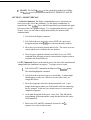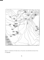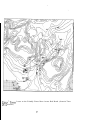
1
NPS-MA-97-007
NAVAL POSTGRADUATE SCHOOL
Monterey, California
19980205 086
Janus Version 6.0 Tutorial
Bard K. Mansager
Gerald M. Pearman
Larry R. Larimer
Michael L. Shenk
1 October 1996 - 30 September 1997
Approved for public release; distribution is unlimited.
Prepared for:
Naval Postgraduate School
Monterey, California 93943
NAVAL POSTGRADUATE SCHOOL
MONTEREY, CA 93943
Rear Admiral M. J. Evans
Superintendent
R. Elster
Provost
This report was prepared in conjunction with research conducted a t the Naval Postgraduate School and
funded by Institute of Joint Warfare Analysis.
Reproduction of all or part of this report is authorized.
This report was prepared by:
&I(.
Bard K. Mansager
Senior Lecturer of Mathematics
M. Pearman
TRAC-Monterey
c
farryik.LarGer
I
TRAC-Ft Leavenworth
Michael L. She&
Mathematics Department
IReviewed by:
R
ea&
el&(
WALTER M. WOODS
Chairman, Depirtment of
Mathematics
D. W. NETZER
Associate Provost and Dean of
Research
-
Form Approved
OMB NO. 0704-0188
REPORT DOCUMENTATION PAGE
'UMIC reporting burden for this CollMiOn of information is estimated to average 1 hour per response. including the time for reviewing instruclions. searching existing data sources.
l a t h i n g and maintaining the data d t d . and completing and reviewing the collection of information Send comments r arding this burden estimate or any other aspect of this
Ollsxtion of information, including suggestiom for reducing this burden to Washington Headquanen Services, DirMorate?or Information Operations and Reports, 1215 Jefferson
)ave Highway, Suite 1204, Arlington, VA 222024302. and 7 0 the Office of Management and Budget. Paperwork Reduction Pro]ect(07@4-0188), Washington, DC 20503
3. REPORT TYPE AND DATES COVERED
I. AGENCY USE ONLY (Leave blank)
I
I
Technical Report
-
1 Oct 1996 - 30 Sep
- 1997
5. FUNDING NUMBERS
I. TITLE AND SUBTITLE
Janus Version 6.0 Tutorial
DFR
Bard K. Mansager, Gerald M. Pearman,
Larry R. Larimer, Michael L. Shenk
'. PEWORMING ORGANIZATION NAME(S)
8. PERFORMING ORGANIZATION
REPORT NUMBER
AND ADDRESS(ES)
Naval Postgraduate School
Monterey, CA 93943-5000
NPS-MA-97-007
I. SPONSORING I MONITORING AGENCY NAME(S) AND ADDRESS(ES)
10. SPONSORING /MONITORING
AGENCY REPORT NUMBER
Institute of Joint Warfare Analysis
Naval Postgraduate School
Monterey, CA 93943
I
1. SUPPLEMENTARY NOTES
2a. DISTRIBUTION / AVAILABILITY STATEMENT
12b. DISTRIBUTION CODE
Approved for public release; distribution is unlimited.
3. ABSTRACT (Maximum 200 words)
A self-paced tutorial is presented using the Janus (version 6.0) high resolution combat model. Utilizing
a scenario incorporating air, sea and land forces in a coordinated amphibious landing, the student is
introduced to rudimentary use of the model. The goal is to become quickly familiar with the model and
be able to construct a simple scenario. The tutorial is intended to be a first step which efficiently teaches
the student basic model use.
4. SUBJECT TERMS
15. NUMBER
Autonomous Legged Underwater Vehicle, Crabs, Mine Countermeasure,
Janus
7. SECURITY CLASSIFICATION
OF REPORT
JNCLASSIFIED
SN 7540-01-280-5500
18. SECURITY CLASSIFICATION
OF THIS PAGE
I
UNCLASSIFIED
19. SECURITY CLASSIFICATION
OF ABSTRACT
I UNCLASSIFIED
,6.
.
F PAGES
99
CODE
20. LIMITATION OF ABSTRACT
I
Standard Form 298 (Rev 2-89)
Prescribed by ANSI Std Z39-18
298.102
Janus Version 6.0 Tutorial
Bard K. Mansager
Mathematics Department
Naval Postgraduate School
Monterey, CA 93943
Gerald M. Pearman
TRAC-Monterey
Monterey, CA 93943
Larry R. Larimer
TRAC-Ft Leavenworth
Ft. Leavenworth, KS 66027
Michael L. Shenk
Mathematics Department
Naval Postgraduate School
Monterey, CA 93943
December 1997
Abstract
A self-paced tutorial is presented using the Janus (version 6.0) high resolution combat model. Utilizing a scenario incorporating air, sea and land forces in a coordinated
amphibious landing, the student is introduced to rudimentary use of the model. The
goal is t o become quickly familiar with the model and be able to construct a simple
scenario. The tutorial is intended t o be a first step which efficiently teaches the student
basic model use.
1
1NTRODUC.TION
Joint warfare analysis experts must have a sound background in the use of combat models.
In an environment impacted by changing weapon systems, doctrine and tactics, modeling
is the centerpiece for analysis. High resolution modeling provides the warfare specialist an
opportunity t o examine the effects of new technologies on the joint battlefield long before
the development of the actual system. Additionally, high resolution modeling provides a
method to evaluate new doctrine and tactics and their impact on the battlefield. A graduate
of the joint warfare curriculum must have a firm grasp of the capabilities and limitations of
models to make sound decisions for the 21st century force.
RESEARCH OBJECTIVES
The goal of this research is to provide a methodology enabling a student to quickly become
familiar with a combat model. The main product of this research is a tutorial allowing a
student to learn how Janus works. (Appendix A). Although this familiarity is rudimentary,
the student can use this introduction to expand his knowledge of high resolution models as
the need arises. The J a m s model, version 6.0, is the model of choice for this study although
the same methodology applies to other high resolution models.
BACKGROUND
Janus is the premier high resolution model used by the U. S. Army. It is named after the
two-faced Roman god who guards portals. Janus is an interactive, work station based, wargaming simulation used for combat operations at brigade level and below. Janus is developed,
maintained and distributed by the U. S. Army TRADOC Analysis Center, White Sands
Missile Range, New Mexico (TRAC-WSMR). The model is fielded throughout the armed
forces as a tool for trainers and analysts for testing, research and combat development. The
model operates on the UNIX-based Hewlett-Packard work station.
Janus is capable of simulating water, weather, rotary and fixed wing aircraft, day and
night visibility and obstacles. The model uses line-of-sight (LOS) algorithms to detect targets
and makes provisions for several detection leaves, e.g. detect, recognize and classify. A
target must be within both LOS and a weapon’s range in order for an engagement to occur.
Engagement outcomes are then determined from probability of hit (Ph) and probability of
kill (Pk)tables in the database. The Ph and Bk data used are representative of capabilities of
actual weapons and are produced by TRAC-WSMR and the Army Material Systems Analysis
Activity (AMSAA). Distinct Phs and Pks are provided depending upon the posture of each
force (stationary/moving, exposed/defiiade and flank/head-on exposure).
The J a m s terrain database is a digitized representation of real world terrain and was
distributed by the National Imagery and Mapping Agency (NIMA) and the Waterways
Experimentation Station (WES), Vicksburg, MS. The data is converted from a profile plot
to a contour plot for use in the Janus model. Within Janus, the user can initialize the
size of the exercise area based upon his needs. The represented area is a square that is
subdivided into 360,000 (600 x 600) grid cells. The size of each grid cell is referred to as the
2
“resolution” of the terrain. Commonly used resolutions are 25, 50, and 100 meters which
correspond to an overall exercise area of 15, 30 or 60 square kilometers, respectively. This
research used 100 meter resolution. Assigned to each grid cell are characteristics existing
within its boundaries including elevation, vegetation, roads, water and urban areas. These
characteristics are homogeneous throughout the cell. For example if the elevation assigned
is 100 meters then the entire cell is at an elevation of 100 meters. Terrain impacts movement
and LOS calculations within the model’s algorithms. A more detailed description of the
model can be found in [l].
SCENARIO
A scenario employing land, air and sea forces is used to stimulate the student’s interest
and to place him into a familiar operational environment. The scenario consists of an amphibious assault at Red Beach, Camp Pendelton, California. In the simulation, the Blue force
(friendly forces) consists of both fixed and rotary-wing aircraft, ships for both transport and
naval gunfire support, landing craft and amphibious assault vehicles (AAVs) supported by
tanks. The Red force (enemy forces) consists of antiaircraft weapons, barriers, dismounted
troops with antitank weapons, personnel carriers, artillery and tanks. Appendix B contains
Janus screens at various stages of the battle.
The scenario’s general time sequencing is as follows:
a. 0-15 minutes: The Red force conducts patrolling operations in the vicinity of Las
Pulgas Canyon overlooking Red Beach and the areas surrounding Camp Pulgas. Air defenses
are in a layered defense, beginning at Red Beach and ending in the hills northeast of Camp
Pulgas. Red artillery is positioned in the hills to the east of Camp Pulgas.
b. 16-25 minutes: The Red force observes the amphibious assault force approaching
approximately four kilometers off shore, moves into hasty defensive positions and calls for
artillery support. The Blue force uses naval gunfire to suppress enemy activity on the
hills overlooking Red Beach. AH-64 Apache helicopter gunships approach Camp Pendelton
south of Red Beach and proceed inland following Santa Margarita River. Fixed wing aircraft
approach Camp Pulgas from the northwest along San Onofre Canyon. Red air defense forces
observe and fire on the Blue air assets. The Apache helicopters engage Red artillery t o
neutralize their effectiveness prior to the forthcoming amphibious assault.
’
c. 26-30 minutes: Blue fixed wing aircraft engage Red air defense forces to the northeast
of Camp Pulgas. The AAVs begin their assault onto Red Beach, firing at enemy positions
overlooking the beach. Naval gunfire shifts from the area of Red Beach to the Camp Pulgas
objective area.
d. 31-45 minutes: Enemy forces hold their positions although incurring heavy losses.
The AAVs maneuver across Red Beach and secure an area for the following Landing Craft
Air Cushion (LCACs) to land. The LCACs unload an M1 tank on 1an.d and then return
to the open ocean. The Apache gunships join the attack force on the beach and together
continue to attack into Las Pulgas Canyon toward Camp Pulgas. A squad of AAVs move
into an overwatch position in the high ground to the southwest of Eas Pulgas Canyon.
3
e. 46-60 minutes: Blue and Red forces located in the objective area begin to exchange
fire. The Blue force begins its final assault on the objective.
CONCLUSION
This tutorial provides the student with an adequate introduction to the Janus 6.0 model.
It will familiarize him/her with the basic mechanics of the model and allow the user to
rapidly develop a simple combat scenario. The goal is to start using the simulation quickly
and in the most efficient manner.
REFERENCES
1. Department of the Army, “Software User’s Manual, version 6.3, UNIX Model,” Simulation, Training and Instrumentation Command, Orlando, Florida.
2. Department of the Army, “Database Manager’s Manual, version 6.0, UNIX Model,”
Simulation, Training and Instrumentation Command, Orlando, Florida.
4
APPENDIX A
- JANUS TUTORIAL
5
JANUS TUTORIAL 1
1. INTRODUCTION
The amphibious task force commander clears his throat and everyone comes to order.
The commander begins, “You’ve all been briefed on the situation. Make sure you
understand my intent. I want a deep helicopter strike to the south followed by an
amphibious landing in the center supported by naval gunfire. In the north, rotary and fixed
wing air assets will conduct a supporting attack., . . . Commanders and staffs can train for
such a scenario using Janus, a legacy simulation which possesses many proven features.
”
2. JANUS OVERVIEW
Janus is a high resolution interactive ground combat computer simulation. It allows you
to simulate the combat interaction of friendly and enemy forces. Each element is viewed
on the Janus screen as an icon. The icon may represent one or more pieces of equipment.
For example, one icon may represent one tank, or it may represent a platoon of tanks. This
tutorial will show you how to tell the difference.
3. TUTORIAL OVERVIEW
This document is a tutorial for the beginning Janus user on the HP workstation. We
provide a step-by-step method to learn the fimdamentals of Janus quickly. The first time
user should follow the tutorial in sequence. The more experienced user can skip any
section that is not relevant. This document does not cover all hnctions of Janus. We
introduce the basic fimctional commands and features of the model that allow you to use
Janus as a research tool.
4. COMMANDS
During the execution of Janus, the primary input method for commands is a three-key
mouse. The three-key mouse and the keyboard provide four basic Janus command inputs
6
The 3-key mouse has four
control outputs. Each key
performs a separate control
function. Viewing the mouse
from above, the left key is
the #1 key, the center key is
the #2 key, the right key is
the #3 key, and any key
together with the “shift key”
on the keyboard is the #4
key.
4 - “shift key” + any mouse key
The Janus users manual assigns colors to these mouse command fimctions:
#1 key #2 key #3 key #4 key -
white key
yellow key
blue key
green key
We will use the following commands and terms frequently in this tutorial:
“left click”
-
(the most common control function) press the #1 key.
“center click”
-
press the #2 key.
“right click”
-
press the #3 key.
“shift click”
-
press any key while holding the shift key down.
“double click”-
press the appropriate key twice rapidly.
a graphical representation of a piece of equipment. The
“icon”
icon may represent one or more elements. For example, one icon may represent a platoon
of tanks or only one tank.
Cl.
icon window”-
a klly reduced window (looks like an icon).
7
We will often use the preceding control hnctions together with a reference to a specific
icon, command hnction, or geographic feature. For example: “left click an icon” means
to move the mouse on its pad until the screen cursor is positioned on an icon, then press
the left mouse key.
5. OTHER COMMANDS
There are two “enter” keys on the keyboard. In Janus, these keys have different functions.
We will refer to the enter key located in the main section of the keyboard, usually just
above the right shift key, as the “return” key. We will refer to the other enter key, located
in the expanded section of the keyboard on the numeric keypad at the far right, as the
“enter” key.
6. LOGGINGON
Each HP terminal in the computer lab is associated with a specified number of Janus
workstations. Before logging-on, you must know the workstation numbers for your
terminal. Make note of the workstation numbers because they will become important later
in the tutorial. (Your workstation number is located in the XASSIGN.DAT file in the HP
file manager).
Note to first time UNM users: If at any time while in an “hpterm” or “xterm” window
(these windows are described later) and you are unable to make the screen respond to
your commands, the screen appears to freeze, or you have generally lost control of the
situation, push the “control” key and the “C” key at the same time. This will terminate
any program that is currently running and allow you to start over from the beginning.
To log-on: With the mouse, left click on the space provided for your username. The
blinking cursor should now appear in the leftmost area of the username space. Type your
username in the space provided and press the ‘tab’ key on the keyboard. The blinking
cursor should now appear in the space provided for your password. Type your password
in the space provided and press the return key.
At this point, two different environments may be encountered depending upon the Janus
configuration of the HP workstation. If the Janus User Options window depicted on the
following page does not appear immediately after logon, then continue with the
instructions listed below. Following these instructions will produce the Janus User
Options window.
A U. S. Government warning message should appear with an hourglass ‘icon’ in the
center of the screen followed shortly by an HP ‘desktop’ screen. At the extreme bottom
of the desktop and just to the left of center, there is a computer console icon (looks like a
computer). Left click on this computer icon. A window should appear with the word
“hpterm” centered at the top (this is called an hpterm window). At the top of the hpterm
8
window there is a prompt (‘‘
followed
3 by a blinking cursor. Type the word “xterm”
(no quotation marks) and press the return key. (See below.)
hp 1>xte r m
(return)
Now a new window will appear labeled “xterm” (this is an xterm window).
After the xterm window opens, you may now minimize the hpterm window using the
following procedure:
1. Left clicking on the ‘‘0’’ at the upper right corner of the hpterm window (next
to the small box in the extreme upper right corner).
2. The hpterm window should reduce to an icon window which is at the upper
left corner of your screen (labeled “hpterm” at the bottom).
Return to the xterm window by left clicking anywhere inside of it. Now type “menu” as
shown below and press the return key:
hp l>menu
(return)
This will start Janus and the following Janus User Options window will appear:
9
You are now logged-on and ready to proceed in Janus.
7. JANUS ADMINISTRATIVE COMMANDS
This main Janus menu screen lists several command options, two-letter option codes, and
a user prompt at the bottom of the screen which reads “Enter Option”. For this tutorial,
we will only be concerned with the “Program Execution” option which has the two-letter
code “PE’. Type “PE7at the Enter Option prompt and press the return key as follows:
E n t e r Option:
PE
(return)
The following Program Execution screen will appear:
This screen allows you to edit and adjust many aspects of the scenario prior to a run. For
now we are only interested in the “Janus Execution” option (two-letter code “JE”). Type
“JE” at the Enter Option prompt and press the return key as follows:
E n t e r Option:
JE
(return)
The following line should appear in the xterm screen that you started earlier:
E n t e r t h e S c e n a r i o Number f o r t h i s r u n (1-999): [
1
Highlight the xterm screen by moving your mouse pointer anywhere on the xterm screen
and left click once. This tutorial was designed around scenario 3 11, an amphibious landing
at Camp Pendleton, CA, so this is the scenario we recommend. This scenario number is
not specific to the Janus environment, so the actual scenario number assigned to this
simulation may be different. Verifl the scenario number assigned to the Camp Pendleton
10
simulation with the system administrator. Without loss of generality, this tutorial will
reference “3 11” as the appropriate scenario. Enter the number of the scenario inside the
square brackets and then push the return as follows:
E n t e r t h e S c e n a r i o Number f o r t h i s r u n (1-999): 13111
(return)
A new line will appear asking for a run number between 1 and 99. The “run number” is an
administrative control that allows you to vary your scenario and capture output from
different variations in separate output files. For now, the run number you select is not
important. We recommend run number 1. Enter the appropriate number in the square
brackets and press the return key as follows.
E n t e r t h e Run Number f o r t h i s r u n (1-99): [ O l ]
(return)
At this point there are two possible outcomes:
1. Two new lines appear which read:
RUN number XXX h a s a l r e a d y b e e n made.
E n t e r XX t o s t o p , o r p r e s s ’ RETURN t o c o n t i n u e [
]
If this occurs, a previous student has run the scenario using the same run number that you
just inputted. Simply press the return key to continue (you will write over the previous
student’s output file, but that’s OK).
2. One new line appears which reads:
E n t e r XX t o s t o p , o r p r e s s RETURN t o c o n t i n u e [
1
If this occurs, simply press the return key to continue.
Next, a Janus Run Types Menu will appear which prompts you to select a run type. We
want a NORMAL Run, so type a “1” at the Select Run Type and press the return key as
follows:
Select Run Type [ 1 ]
(return)
Now, the xterm window will display lines indicating that files are being read by the HP
system, and a new menu will appear titled “Janus RUNTIME SCREENS”. The window
looks as follows:
11
This screen allows you to review information about friendly and enemy forces associated
with this specific scenario, allocate Janus workstations, allocate obstacle resources to
units, and review some of the parameters Janus uses to operate. Additionally, we will
start our Janus run from this screen. For now, we are only concerned with Janus work
station assignments, and starting the simulation.
Select SCREEN I1 : Work Station Assignments option (two letter code “2Z”), enter the
code by typing “22” at the Select Option prompt, and press the enter key (this is where we
begin to use the numeric keypad enter key):
Select O p t i o n -- > 2 2 (enter)
The screen will now change to “Janus SCREEN II”. This screen allows the user to set
the proper work station numbers so that the friendly and enemy forces in your scenario
appear on your monitor. Make your screen look as follows:
12
You must verify that the two work station numbers you were given are listed in the WS
Number columns and that these two work station numbers correspond to Side 1 (friendly
forces), and Side 2 (enemy forces). For example, if your work station numbers are 1 and
5, then there should be a “1” and a “5” in the WS Number column with either a “1” or a
“2” in the Side column for work station 1, and a “1” or a “2” (whichever is not associated
with work station 1) in the Side column for work station 5. If the workstation numbers do
not match yours, change them. (Janus is capable of playing up to six sides. Ensure
workstations are properly assigned when playing multiple sides). Press the return key and
the blue blinking cursor will cycle through the positions on the screen. If you go too far,
you can use the “backspace” key to cycle backwards through the positions (or you can
move the mouse pointer over the location of the option you need to change and left click).
When the blue blinking cursor is over the number to be corrected, type in the correct
number.
NOTE: You cannot assign two “sides” to one work station. You should have at least
two work station numbers and each of these numbers should be assigned a different
“side”.
The “GI-OU~”,
“Symb Size”, and “Graph Tablets” positions should be assigned the
numbers “l”, “9”, and “l”,respectively (just as you see in the screen representation
above). If they are not correct, change them to the appropriate numbers. (See chapter 6,
Software User’s Manual, Version 6.3, for descriptions of “Group”, “Symb Size”, and
“Graph Tablets”).
When all work station numbers are correct, then press the enter key. This will return you
to the Jams RUNTIME SCREENS menu.
13
8. PREPARATION FOR MAP ENVIRONMENT
You are now ready to enter the map environment. Find the two-letter code for “Begin
Janus” (it should be “JJ”), enter the code at the Select Option prompt and press the enter
key:
S e l e c t Option
-- >
JJ
(enter)
At this point you will see in the xterm window that Janus is reading the terrain files and
setting up the “Battlefield Graphics windows.” You will know that the setup is complete
when the following two conditions are met:
a. The text in the xterm window will read:
S c e n a r i o XXX Forces:
DF
Total
Units U n i t s Units
30
147
177
165
178
13
Arty
Side
1
2
NOTE: Your numbers may not match the above example - they are scenario
dependent.
b. An “icon window” will appear for each of the “sides” you set up in the Janus
Workstation menu. For example, if you are running a scenario with “side 1”
and “side 2”, and you set up Janus Screen I1 (Workstation menu) to display
both “sides” on your Hp workstation, then there should be two icon windows
in the upper left corner of the screen labeled “side 1” and “side 2”.
2. HIGH RESOLUTION BATTLEFIELD GRAPHICS
Note: Janus uses digitized terrain developed by the Defanse Mapping Agency (DMA).
The terrain appears in a form familiar to military users displaying elevation contours,
roads, rivers, vegetation, and urban areas. The colors used in the model are slightly
different than used on military topographic maps; elevation contours are brown, rivers
and other bodies of water are blue, roads are brown or gray with white outlines, urban
areas are yellow and vegetation is green. Other features such as pipelines, power lines,
railways and fences can also be portrayed.
Now, double left click on the icon labeled “side 1”. The resulting window should look
similar to the figure below. The right side of the screen is an interface panel which you
will use to control the forces displayed on the map.
14
You can “resize” the battlefield graphics screen by moving the mouse pointer to the upper
right comer of the screen until the pointer changes to a “corner symbol”. When the comer
symbol appears, left click with the mouse, hold the key down, and move the mouse to the
left and down to make the screen smaller. We suggest you shrink the side 1 screen to fit in
the lower left corner of the monitor.
Now, double left click on the icon labeled “side 2”. The resulting window displays the
side 2 initial positions just like the side 1 screen. You can also resize this screen in the
same manner that you resized the side 1 screen. We recommend you grasp the upper left
hand comer of the side 2 screen and move it to the lower right corner of your monitor
workspace. Your computer monitor should now look like this:
i
xterm
-..
window
‘i
I
You are now ready to issue initial “orders” to the units on the screen. Further instructions
for deployment, assignment of sectors of fire, establishment of routes, etc., will be covered
in the next section of this tutorial.
10. SCENARIO PREPARATION COMMANDS
The following section describes the Janus interface panel. It will explain how to input
commands to battlefield units. The scenario we are working with (scenario 3 11) portrays
an amphibious assault landing at Camp Pendleton, CA. The landing force (side one) is
composed of several battlefield systems, including Amphibious Assault Vehicles and
LCACs each carrying an MI tank. The defending force (side 2) consists of tanks, air
defense weapons, and barriers positioned in a valley along the coast of Camp Pendleton.
Enlarge the side 2 Battlefield Graphics Window and familiarize yourself with the position
of the forces. Note that there are three entities in the upper left hand corner of the screen.
There is a T-80 tank, an artillery piece, and a find helicopter. You will be experimenting
with the Janus Interface Panel commands using these battlefield systems. These
instructions will guide you through each command and familiarize you with operating in
the Janus environment. You should read through section 1 (administrative commands) of
the Interface Panel and then move on to section 2 (maneuver plan) where you will begin to
input commands to the units on the battlefield.
,
At this time, you may want to run the Camp Pendleton scenario so that you can
visualize what a complete Janus scenario run looks like. In order to do this, go to
paragraph 14 (Start Simulation) on page 23 of this tutorial. Follow the start steps and
watch the complete amphibious assault. When all the action is complete (approximately
simulation time 75:OO) or when you have seen enough action, stop the simulation using
the procedure outlined in paragraph 15 (Stop Simulation and Log Off) on page 23.
Paragraph 15 also outlines the correct log off procedure you will follow at the conclusion
of your Janus session.
16
11. JANUS INTERFACE PANEL
Before beginning any scenario, the user must take certain
preliminary steps. To enable the user to do so, Janus
displays options along the right side of the screen in the
form of the menu you see here (the Janus Interface Panel).
The commands are selected by moving the mouse cursor
over the command and clicking the left mouse key. This
menu appears at the right of the terrain map for both side 1
and side 2 forces. The menu has the five sections listed
below:
a. Administrative (TASK, MINE DENSITY, FLIGHT
MODE, TIMER)
b. MANEUVERPLAN
c. STATUS
d. A R T Y P L A N " G
e. Administrative Screen Control
f. CLOCKS
SECTION 1 - ADMINISTRATM
a. TASK. The five numbers to the right of TASK
are the task force numbers of units on the
screen. Pick one of these numbers to display
that task force number slightly above and to the
right of the unit symbol. Try this command by
choosing Task 1 or 2 on either the side 1 or side
2 window. You should see small numbers
appear by various icons on the map.
7
L.mm
&%iY$
Paw N F X : F!
?4....I ....:.......
.i I....i....i....L ....:....1.....L..* ....i
....
...
:.>:.F.\P ;r: P I 3 H1t.F
.I
b. MINE DENSITY. The three options in this section are: L for low (40
mines), M for medium (80 mines), and H for high (160 mines). They refer to
the density in a 50,000m2 area. Mine density applies to FASCAM and
vehicle-emplaced minefields, but not to hand-emplaced minefields.
C.
FLIGHT MODE. Flight mode 1 causes aircraft to fly low and slow and flight
mode 2 causes aircraft to fly high and fast.
d. TIMER. The TIMER function is used with other fbnctions to plan fbture
events such as prearranged artillery fire or scheduled unit movements.
e. ENG AREAS ON. When enabled, this function activates engagement areas
for direct fire weapons. Units will engage other units within engagement areas
according to the firing criteria specified previously on Janus Screen IV.
17
f
FLOOR. The FLOOR fbnction sets the current floor number for buildings.
This function is used in conjunction with MOUNT, DISMOUNT, and LOS.
SECTION 2 - MANEUVER PLAN
a. DEPLOY Command: The Deploy command allows you to reposition your
forces prior to the start of the simulation. Use the deploy command now to
reposition the Tank, Artillery Piece, and Helicopter that are positioned in the upper
left corner of the side 2 graphics display. You can place them wherever you like
for now. Later, you will want to deploy them tactically for inclusion in the
simulation battle.
1. Left click on the Deploy command.
2. Left click on the icon you want to move (NOTE: the cursor cross
disappears and the mouse freely moves the icon about the window).
3. Move the icon to the new position and left click. The cursor cross now
returns and the icon is located at the new position.
4. Do not forget to check the element’s new field of view (see VIEW
command in the following section) to ensure that the weapon system is
oriented in the desired direction.
b. EXT Command: Routes can be entered prior to the start of the simulation and
changed while the simulation is in progress. To assign a route to a unit:
1. Left click the EXT command in the Maneuver Plan fimction group.
This should highlight the command.
2. Left click on the icon whose route you are building. A white triangle
should appear over the icon. Wherever you move the cursor, an
orange line follows.
3. Move the orange line to the next checkpoint and left click. A new
triangle should appear where you clicked with a white line connecting
the two triangles. In this way you can plot routes as a succession of
straight line segments.
4. At the final checkpoint for the route, center click. This will end the
route planning for that unit and the orange line that follows the cursor
will be turned off
5. Refer to the ALT and DEL commands, Sections 2b. and 2c.
respectively, to alter or delete a route.
18
When you are finished setting routes, left click the “CLEAR” command in section 5 of the
Interface Panel to clear the screen of all route lines. Try creating routes for each your
three battlefield systems on side 2.
NOTE: There are two different types of white triangles which form the corners of your
routes.
1. A GO triangle looks like the one shown here:
2. A STOP triangle looks like this:
3. STOP triangles are designed to hold unit at th stop location for
specific
period of time before the unit is allowed to move to the next leg of its route.
Timed triangles are beyond the scope of this tutorial.
4. To change a STOP triangle to a GO triangle (or vice versa):
Left click on the EXT command.
0
Left click on the icon you wish to change. This displays the icon’s
current route.
Right click on the triangle you want to change from a STOP to a GO
triangle. The triangle should change to a GO triangle. The same
procedure works for changing a GO triangle to a STOP triangle.
c. ALT Command: Allows you to alter a previously entered route.
1. Left click on the ‘‘ALT’?Command. This should highlight the
command.
2. Left click on the icon whose route you wish to alter. The icon’s
current route will be displayed in white.
3 . You may now left click on, and move any triangle except the one
covering the icon.
4. Place the triangle in the new location and center click.
19
d. DEL Command: Allows you to delete a single leg from a previously entered
route.
1. Left click on the “DEL” Command.
2. Left click on the icon whose route you want to alter. The icon’s
current route will be displayed in white.
3. Left click on the triangle you want to delete and it will disappear
leaving that portion of the route that exists without the triangle you
deleted.’
e. CAN Command: If you want to cancel a route:
1. Left click the task force number of the unit you wish to affect.
2. Left click the “CA”’ command. The command should be highlighted.
3. Left click on the icon whose route you want to delete. The current
route will apper in white. Left click again and the route should be
removed. The unit becomes stationary.
f SHOW Command: If you want to view the routes again:
1. Left click the task force number of the unit whose route you want to
see: The number should be highlighted and task force numbers will
appear over all units on the simulation screen that are part of that task
force.
2. Left click on the “SHOW’ command. The assigned routes for the task
force you’ve selected will be displayed in orange.
g. XINL Command: Allows you to give different icons the same route so that
they follow behind one another (not needed for this tutorial).
h. XONLCommand: Allows you to give different icons the same route so that
they move abreast (not needed for this tutorial).
i. STOP and GO Commands: These commands allow you to stop an entire task
force’s movement, or start an entire task force’s movement.
1. Left click on.the task forces you want to effect.
20
2. Left click on the GO command and the entire task force will initiate
movement (any current STOP triangles will change to GO triangles).
3. Left click on the STOP command and the entire task force will stop
movement (current GO triangles will change to STOP triangles).
j. LOS Command: Displays an element’s field of view and what it can see (Line
of Sight).
1. Left click on the LOS command. The command should now be
highlighted.
2. Left click on the icon for the element you want to check.
3. A sector arc will appear that shows the line of sight in the field of view
that was last assigned to that unit (see section 3 - View command).
The dashed white line indicates the center of the sector between left
and right lateral limits. The orange lines are areas where vision is
unimpeded while deadspots (areas the element cannot see) are
represented by missing segments in the orange radial lines. The
maximum visibile range of the element is represented by the far white
arc. The maximum range of the primary weapon system is represented
by the purple arc.
4. To check the LOS for a location with no icon, move the cursor to the
new position and click. A full 360 degree field of view will appear. If
you find this position’s LOS to be more favorable, then deploy (see
para 1 below - Deploy command) the unit to the center of the LOS
circle and recheck the element’s LOS to verifjr proper placement.
k. MOUNT Command: Allows you to mount one system on another for
movement and protection (infantrymen to mount in fighting vehicles, tanks to
mount in LCACs, etc.). This hnction will not be used in this tutorial.
1. DISMOUNT Command: Allows you to dismount one system from another.
m. PREPOS Command: Allows you to establish prepared positions that will
increase your elements’ survivability and concealment. Janus will allow you up to
600 prepared positions. The positions are depicted on the graphics screen as
follows:
,,_.-..__
.
Infantry Prepared Position
.
.
‘X.
21
Helicopter Pop-up Position
__...-_
/’
‘.
\
:;-.
-:
:. .. ‘I..<./;;
.,‘,:.
-.. :;
.‘
.%.-_<.
/.’
1. To create a prepared position, left click on the PREPOS command,
move to the location where you want to place the prepared position.
Left click to create an infantry prepared position. Center click to create
a vehicle prepared position. Right click to create a helicopter pop-up
position. If you place a prepared position on top of an icon, the icon is
now in a prepared position.
2. To remove a prepared position, left click on the PREPOS command,
then shift click on the prepared position you want to’remove.
SECTION 3 - STATUS
This section allows you to change several of your units’ parameters, review data
concerning friendly forces, adjust you units’ field of view and other hnctions.
a. UNIT/TASK/BLDG.
The first commands under Status are the Unit/Task/Bldg
commands. These commands determine the scope of the changes you make in
parameters. For example, if you left click on Unit, then left click on NBC,and
then left click on one icon, only that icon will be effected. However, if you left
click first on Task (task force), then on NBC, and then on an icon, 4the
elements in that icon’s task force will be effected. Likewise, if you first left
click on Bldg, any adjustments you make to an icon that is inside a building,
will also effect all other elements that are inside the building.
b. HF. This hnction changes the hold fire status of a unit. If a unit is in a HF
status, that unit will not engage enemy units until HF is disabled. After left
clicking the desired TASK number in section 1, UNIT in section 3, and HF, the
map will display the HF status of the corresponding units. There will be a
white “V” under the icon of units that are in HF status, and a white line under
units that are not in HF status. The user can change the HF status of a unit by
clicking on the unit icon. You can change an entire task forces’ HF status by
highlighting TASK (instead of UNIT) prior to clicking on the unit icon.
c. NBC. If NBC is enabled (“V” displayed), the unit is in protective gear. NBC
status is enabled/disabled similar to HF.
22
d. BRE. If BRE is enabled (“Vdisplayed), those units with breach capability
will begin conducting breaching operations, even if no minefield/obstacle is in
the vicinity of the enabled unit. Breaching units move slower than nonbreaching units. BRE status is enabled/disabled similar to HF.
e. SPR. If SPR is enabled (“V’displayed), those units are in a sprint mode and
will move at maximum possible speed. SPR does not affect flying units. SPR
status is enabled/disabled similar to HF.
f
DEFL. If DEFL is enabled (77“ displayed), those units are in full defilade.
When in full defilade, the unit cannot engage enemy units except in self
defense, although they can see the enemy. Units in full defilade are not visible
until the enemy is within 50 meters. Units in partial defilade (white line
displayed) will engage the enemy. DEFL status is enabled/disabled similar to
HF.
g. REPORT KILLS. Selecting KILLS displays original number of friendly
systems by type, remaining systems, system losses, and total losses. Selecting
KILLS with the center mouse key gives information for selected task force.
Selecting KILLS with the left key gives the same information for all forces
assigned to the workstation. Selecting KILLS with the right key gives the
same information for the entire side.
h. REPORT TF. Selecting TF with the center mouse key displays a text report
on the currently selected task force. Selecting TF with any other mouse key
displays the unit number of each unit in the selected task force on the map
below the icon.
1.
REPORT INFO. Selecting INFO and selecting a specific icon with the center
mouse key, displays the same text report as TF for the selected icon. Selecting
an icon with the left key displays the unit’s grid location. Selecting an icon
with the right key displays the unit’s routes. Selecting an icon with the shift
click key displays the unit’s ammunition status.
j.
FRIENDS. When the user plays fratricide, Janus disables FRIENDS. When
the user does not play fratricide, the FRIENDS report displays all same-side
units assigned to other workstations and all different side units that are not
enemies, if line of sight exists between them and a unit of your workstation.
k. ARTY. Selecting ARTY with the left, center, or right mouse key displays
currently planned artillery missions. Selecting ARTY using shift click displays
all target reference points.
1. INTEL. Selecting INTEL with the center mouse key draws a line between the
detecting units and all units they currently detect. Selecting INTEL with the
23
left key displays the last 25 units detected within the last ten minutes which are
no longer detected. Selecting INTEL with the right key displays aggregation
level and formation of each currently detected unit.
m. CLDS. Janus can simulate smoke pots. The user inputs smoke into the
scenario using JANUS SCREEN 111. The smoke pot symbols are a square
with a smoke insignia inside. Smoke pots are deployed during the preparation
phase of the scenario using the DEPLOY command. The smoke pots must be
activated after you start the simulation by clicking the.SETOBS command and
then clicking on the smoke pot symbol. After clicking on the smoke pot
symbol, the symbol will disappear. The CLDS command allows the user to
turn the smoke display on and off When you activate CLDS, all smoke clouds
appear on the screen in the form of a circle. When CLDS is off, no smoke
symbols appear on the screen, but smoke is still in effect.
n. ROTATE VIEWLFORM. These functions allow the user to orient unit view
fans and unit formations. Select the desired function, then select the unit icon
to be adjusted. Adjust the view or formation by positioning the cursor in the
desired direction on the map and clicking the center mouse key.
0.
BAR. Janus can simulate three different barriers/obstacles. They are road
craters, abatis, and minefields. The user inputs barriers/obstacles into the
scenario using JANUS SCREEN 111. Minefields are represented by
rectangular with dimensions as set in the database. Road craters are
represented by two diagonal slashs inside a circle. Abatis are represented by
an upside down “V” with an attached line. Barriedobstacles are deployed
during the preparation phase of the scenario using the DEPLOY command.
Prior to deploying the barriers/obstacles, the user should set their orientation.
To set orientation, first click the BAR command. Notice the small white circle
in the bottom right corner of the window. The circle represents the barrier’s
radius and the white line represents the barrier’s orientation. Moving the
cursor to any point on the circle and clicking on the circle changes the barrier’s
Orientation. Now deploy the barrier/obstacle by clicking DEPLOY and moving
the cursor to the barrier/obstacle you wish to deploy. Click that
barriedobstacle and move the cursor to the desired location on the map and
click again. The barrier is then deployed with the previously set orientation.
Both abatis and road craters must’be activated after you start the simulation by
clicking the SETOBS command and then clicking on the abatis or road crater
symbol. Notice that both abatis and road crater turn from white to purple after
activation.
p. GROUP RE-ORG. This hnction allows the user to change a unit’s task
force number. Select the desire TASK number, select RE-ORG, then select
the desired unit icon. Janus will display the new task force number next to the
24
selected icon. RE-ORG may also be used to transfer units from one
workstation to another.
q. ENG AREAS CREATE. To create an engagement area, select CREATE and
left click on the desired map locations to define the area. Middle click on the
final point.
r. ENG AREAS DELETE. To delete an engagement area, select DELETE
then select the desired engagement area.
SECTION 4 - ARTILLERY PLANNING
This section describes the basics of how to plan artillery. We will ignore most of the
commands under artillery planning since they are beyond the scope of this tutorial. For
this simulation, you will fire only HE, no timed missions, no priority targets, and no
converging sheafs. You will use the Janus Battlefield Graphics window along with the
Artillery Planning section of the interface panel. Experiment with these commands using
your artillery piece. Note: In order for your artillery piece to receive and fire missions, it
must be at a stop triangle (see maneuver plan section and ensure your artillery piece is at a
stop triangle before proceeding).
a. PLAN Command: This command allows you to set-up fire missions.
1. Left click on the PLAN command. It should now be highlighted and
artillery capable elements on the battlefield are hghlighted with a white
X as below:
2. Left click on one of the artillery capable icons and two concentric
circles will appear with the icon at the center. The large circle
represents the maximum range of the artillery piece for high explosive
munitions. The small circle represents the danger close distance (an
artillery piece will not fire within this small circle).
3. Move the cursor away from the artillery piece. Note that an orange
line connects the cursor to the artillery icon. Choose a target that is
outside of the small (danger close circle), but inside of the large
(maximum range) circle. Left click on the target. The orange line now
25
disappears and a white dashed line appears in its place. Additionally,
there is now a target reference point at the target location with a fire
mission number next to it. The artillery element you picked will fire
this mission first when the simulation is started, followed in sequence
by any additional fire missions you add.
b. CANCEL Command: This command allows you to cancel a previously
planned fire mission.
1. Left click on the CANCEL command.
2. Left click on the icon whose fire mission you want to cancel. The
white circles will appear along with the lines and target reference points
which represent that artillery piece’s fire missions.
3. Identifjr the mission you want to cancel and left click on the target
reference point which represents that mission. The mission should
disappear (it is now cancelled).
c. To exit the artillery planning mode, left click on any of the commands in the
MANEUVER PLAN command group (section 2).
SECTION 5 - ADMINISTRATIVE CONTROLS
a. ZOOM. This hnction allows you to magnifl portions of the map. Select the
desired magnification by clicking on the zoom scale then click on the map
location to be magnified. The counter next to ZOOM indicates the zoom
scale.
b. PREVLNEXT. These functions allow you to easily switch between the
previous (PREV) screen and the original (NEXT) screen.
c. M. This fbnction corresponds to the standard military map scale of 1:50,000.
Select Mythen click on the desired map location. The resulting screen will be
in the standard military map scale.
d. CLEAR. This fhction removes temporary text, displays, and graphics from
the screen.
e. GRID. This function superimposes a UTM grid system on the screen.
f
HELP. When this fimction is selected before another menu option, Janus will
display a brief explanation of that option.
26
g. ADMIN. Right clicking on the ADI" function displays an administrative
menu. Menu options include saving the prepared plan, increasing the scenario
speed, or ending the scenario.
h. CAC. This function allows the user to draw Command and Control graphics
on the screen.
i. START. When this finction is selected, the Planning Phase ends and the .
Execution Phase begins. All workstations must pick START before the
Execution Phase may begin.
.
SECTION 6 - CLOCKS. This section displays the simulated time of day in 24-hour
form, and the elapsed time in minutes and seconds from the start of the simulation.
12. SCENARIO PLANNING
You are now ready to input your plan to the units on the screen. This section of the
tutorial includes basic scenario planning. Scenario topics covered include pre-deployment
locations, routes, prepared positions, barrier emplacement, artillery fire missions, and close
air support. (This tutorial assumes that the user has already created the scenario forces in
the force development editor. See chapter 3, Software User's Manual, Version 6.3, for
force development).
'
a. Pre-deployment Locations. When the user develops a new force, the unit icons
are initially placed in a line at the upper right or left corners of the map (you
saw this earlier with your three battlefield systems). Janus places the new force
icons there so the user can easily find and move them to the desired start/predeployment locations. Move the units using the previously described
DEPLOY command on the interface panel (along the right side of the screen)
to tactically appropriate positions given your knowledge of the upcoming
battle. Repeat this process until all pre-deployment locations are set. Ensure
each unit icon is oriented in the proper direction using the LOS and VIEW
commands.
,
b. Routes. Assign routes to unit icons using the EXT command on the interface
panel.
c. Prepared Positions. When preparing a defensive plan, place desired units in
prepared positions utilizing the PREPOS command. Ensure these units have
proper line of sight using the LOS and VIEW commands.
d. Barrier Emplacement. Deploy barriers similar to deploying units using the
DEPLOY command. Ensure that the barriers are oriented in the proper
direction using the BAR command. Note that abatis and craters are not
obstacles until set after the simulation begins.
27
e. Artillery Fire Missions. Use the ARTY PLAN command to plan all artillery
fire missions. This tutorial covers only HE, immediate fire missions. (See
chapter 7, Software User’s Manual, Version 6.3, for Artillery Planning
involving converged sheafs, timed targets, and priority targets).
f
Close Air Support. Select desired FLIGHT MODE command. Select desired
aircraft icon and provide a suitable route using the EXT command.
(Helicopters can be programmed to pop up at points along a route by using the
POP command after the simulation begins. See chapter 9, Software User’s
Manual, Version 6.3, for POP command instructions).
13. PLANSAVE
When you have accomplished all the scenario planning, you may want to save the scenario
positions. Saving the prepared scenario is important if you want to play the same scenario
repeatedly. To save the scenario, click the ADMIN command, then select Plan Save (PS)
or NEW SCENARIO SAVE (NS) from the ADMIN menu. Select desired save option and
return. Janus will return to the map window.
14. START SIMULATION
To start the simulation, select the START command on the interface panel for all “sides”.
The xterm window will appear. The screen will prompt you to type “RR” when ready.
Type “RR”then return. The next prompt is whether you want to perform a PLAN SAVE
now. (This is another method to save the scenario). Type “Y” then return to save the
plan. The screen will then ask for the checkpoint frequency. (Frequency “3” is
recommended. If you are not saving the run, the frequency can be left blank.). Type
frequency then return. This completes the START process and the simulation begins.
You can now experiment with the Janus interface panel commands during the simulation
run.
15. STOP SIMULATION AND LOG OFF
After the simulation run has begun, you may stop the simulation and exit at any time.
Stop and exit the simulation by right clicking on the ADMIN command in section 5 of the
Janus interface panel. This will bring up a window that looks as follows:
28
To end the simulation, enter the two letter code “EJ” at the prompt at the bottom of the
ADMIN window, and press the enter key. This will end the simulation run and bring you
back to the Program Execution screen. Place the mouse pointer anywhere on this
Program Execution screen and right click. Now, you are returned to the Janus User
Options menu. Enter “XX” at the Enter Option prompt at the bottom of the screen and
press return or enter. You have now exited Janus and you should only see the HP desktop
with an icon bar across the bottom of the screen. In the extreme lower right corner of the
icon bar is an icon key titled “EXIT”. Left click on the “EXIT” key and a “Logout
Confirmation” window will appear in the middle of the computer screen. Left click on
“OK’ and the system will automatically log you off and return to “prepared to log-on’’
status. You have now successfblly completed this tutorial.
16. CONCLUSIONS
This tutorial is an adequate introduction to the Janus simulation. It will accustom you to
Janus and allow you to conduct a simple combat scenario. As you become more familiar
with Janus, you may want to explore the more complicated and realistic aspects of the
system.
29
APPENDIX B - GRAPHICAL REPRESENTATION
OF JANUS SIMULATION
-
7.
c igure
I: Friendly Forces at the Start of the Scenario (Scenario Time: 0:QQninutesj
Figure 2: Enemy Forces at the Start of the Scenario (Scenario Time: 0:QQminutes)
32
....................................................................................
..........................................
........................................................................................
............................................
........................................................................................
............................................
...................................................................................................
.................................................
...................................................................................................
.................................................
..............................................................................................................
.......................................................
..............................................................................................................
................................................................
.................................................................................................................................
................................................................
....
............................................................................................................................
................................................................
....................................................................................................................................................
..........................................................................
....................................................................................................................................................
..........................................................................
................................................................................................................................................
........................................................................
................................................................................................................................................
........................................................................
................................................................................................................................................
........................................................................
..................................................................................................................................................
......................................................................
....................................................................................................................................................
..........................................................................
..............................................
.......................
..............................................
.......................
..............................................
.......................
..............................................
.......................
..............................................
.......................
..............................................
.......................
..............................................
..................
................
.......................
..................................
..............................................
.......................
..................................
............................................................................................
..................
................
............................................
..................................
........................................................................................
............................................
..........................................
...................
......................................
...................
......................................
’-..
f
‘9,
’*f
a,*.
%
A;.
...................
......................................
...................
......................................
....................
..................
......................................
......................................
...................
......................................
.. .. .. .. .. ............................
......................................
......................................
:I...................
:;I:1;I:.:I:I:
...................
......................................
...................
......................................
....
....
..................
.........
..I.
.....................................................
................
..................................
.. .. .. .. ............ . . . . .
.....................
. . . .......................................
.. ..... . . . . . . . . . . . ......................
..........
......................................
. . . . . . . . . . . . . . . .. .. .. ..
I
Ti i
Figure 3: Frienciiy Assault Forces at the Start of the Scenario (Scenario Time: O:OO minutes)
33
Figure 4: Closer View of the Enemy Forces at the Start of the Scenario (Scenario Time: G:OO
nli~lutes
j
34
Figure 5 : E n e ~ n ySuppressions and Losses Due to Artillery (Lower Left Corner). Enemy
Suppressions and Losses Due to Fixed W-ing [Top Center! and Rotary Wing [Far Right:
(.Scenario Time: 1 6 0 2 minutes)
35
Figure 6: Coordination of Friendly Forces as They Move Across Red Beach (Scenario Time:
28: 12 mi11::tes)
36
Figuse 7: Enemy Losses as the Friendly Forces Move Across Red Beach (Scenario Time:
28:12 minutes)
Figure 8: Friendly Forcs Suppressions and Losses
Time: 4938 minutes)
38
2s
They Move to the Objective (Scenario
Distribution List
No. of copies
Director
Defense Technology Information Center
8125 John J . Kingman Road.. SFE 8944
Ft. Behoir, VA 22068-6218
2
1)i rect or of Research Admini stratiorL
Code 09
1
Naval Postgraduate School
Monterey, CA 93943
Library
Code 013
Naval Postgraduate School
Monterey, CA 93943
2
Professor Bard Mansager
Code MA4/Ma
Kaval Postgraduate School
Monterey, CA 93943-5216
5
Prcessor Wayne Hughes
Code OR/H1
Navai Postgraduate School
Monterey, C.4 93943-5216
1
Chairman. Code MA
1
Department of Mat hemat ics
Savai Postgraduate SChool
M o ~ t e ~ C-4.
y . 93943-5216
Major Gerald M. laearman
T R A :L'i O l l t erey
c;-
Mon~etrey.CA
93943-5216
-2/ajor Larry R. Larimer
TRAC-Ft. Leavenworth
Ft. Leavenworth, KS 66027
Captal:I(P) Michael L. Shenk
Sava! Postgraduate School
Montetrey, e.4 93943
39