1
Software for Calibration in Gamma-Ray
Spectrometric In-situ Measurements
Master’s thesis in Nuclear Engineering
YE YUAN JOSEFSSON
Department of Chemical and Biological Engineering
CHALMERS UNIVERSITY OF TECHNOLOGY
Gothenburg, Sweden 2014
Software for Calibration in Gamma-Ray
Spectrometric In-situ Measurements
YE YUAN JOSEFSSON
Department of Chemical and Biological Engineering
Chalmers University of Technology
Gothenburg, Sweden 2014
Master’s Thesis
Software for Calibration in Gamma-Ray Spectrometric In-situ Measurements
YE YUAN JOSEFSSON
©YE YUAN JOSEFSSON, 2014
Department of Chemical and Biological Engineering
Division of Nuclear Chemistry
CHALMERS UNIVERSITY OF TECHNOLOGY
SE-412 96 Gothenburg
Sweden
Telephone: +46 (0) 31 - 772 10000
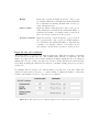
Abstract
A gamma-ray spectrometric measurement on site, or in-situ in Latin, can identify and
quantify the radionuclides after a radioactive fall-out and provide results quickly. The
efficiency of such a measurement, also called the calibration factor, is depending on many
parameters on the site. These parameters may consist of uncertainties, and the quality
of the measurement result is given by the combined uncertainty.
A software, including graphical user interfaces, was developed in MatLab R2014b to
provide the calibration factor and its combined uncertainty for in-situ gamma-ray spectrometric measurements . The field-of-view of the detector was also provided by the
software. Depending on how the radionuclides were deposited on and/or in the soil,
four deposition models were considered in this work. In order to estimate the combined
uncertainty, a numerical approach was used. The samples for each input quantities were
taken according to the Latin Hypercube Sampling (LHS). Moreover, the samples could
be assumed to have either uniform, triangular or normal distribution.
The software gave reliable results about the calibration factor and its combined uncertainty. Also, the detector’s field-of-view that was calculated was reasonable. However
validations need to be performed for some of the models.
keywords: γ-spectrometric in-situ measurement, combined uncertainty,
Latin Hypercube Sampling
i
Acknowledgements
I would like to thank my examiner Chistian Ekberg and my supervisors Henrik Ramebäck
and Torbjörn Nylén for giving me the opportunity to have this interesting project. A
special thank to my supervisors for rewarding discussions and also advice and help they
had given me during the this work. I would also like to thank Patrik Fredriksson for
helping me with the MatLab. Finally, I would like to thank my family and my friends
for their support.
Ye Yuan Josefsson
Gothenburg, January 2015
ii
Contents
1 Introduction
1.1 Background . . . . . . . . . . . . . . . . . . . . . . . . . . . . . . . . . . .
1.2 Purpose . . . . . . . . . . . . . . . . . . . . . . . . . . . . . . . . . . . . .
1.3 Scope . . . . . . . . . . . . . . . . . . . . . . . . . . . . . . . . . . . . . .
1
1
2
2
2 Theory
2.1 Gamma-Ray Spectrometry . . . . . . . . . . . . .
2.1.1 Ground-Level Gamma-Ray Spectrometry
2.1.2 Detector Characteristics . . . . . . . . . .
2.1.3 Field-of-view of a Detector . . . . . . . .
2.2 Radioactivity Deposition Models . . . . . . . . .
2.2.1 Photon Fluence Rate . . . . . . . . . . . .
2.2.2 Multiple Slabs Model . . . . . . . . . . .
2.2.3 Surface Deposition Model . . . . . . . . .
2.2.4 Volume Deposition Model . . . . . . . . .
2.2.5 Exponential Model . . . . . . . . . . . . .
2.3 Statistics and Data Analysis . . . . . . . . . . . .
2.3.1 Monte Carlo Method . . . . . . . . . . . .
2.3.2 Latin Hypercube Sampling . . . . . . . .
2.3.3 Uncertainty Analysis . . . . . . . . . . . .
.
.
.
.
.
.
.
.
.
.
.
.
.
.
.
.
.
.
.
.
.
.
.
.
.
.
.
.
.
.
.
.
.
.
.
.
.
.
.
.
.
.
.
.
.
.
.
.
.
.
.
.
.
.
.
.
.
.
.
.
.
.
.
.
.
.
.
.
.
.
.
.
.
.
.
.
.
.
.
.
.
.
.
.
.
.
.
.
.
.
.
.
.
.
.
.
.
.
.
.
.
.
.
.
.
.
.
.
.
.
.
.
.
.
.
.
.
.
.
.
.
.
.
.
.
.
.
.
.
.
.
.
.
.
.
.
.
.
.
.
.
.
.
.
.
.
.
.
.
.
.
.
.
.
.
.
.
.
.
.
.
.
.
.
.
.
.
.
.
.
.
.
.
.
.
.
.
.
.
.
.
.
.
.
.
.
.
.
.
.
.
.
.
.
.
.
3
3
3
4
4
4
5
8
8
8
9
10
10
11
13
3 Method
3.1 Sensitivity Analysis . . . . . . .
3.1.1 Results and Discussions
3.2 Accuracy Investigation . . . . .
3.2.1 Results and Discussions
.
.
.
.
.
.
.
.
.
.
.
.
.
.
.
.
.
.
.
.
.
.
.
.
.
.
.
.
.
.
.
.
.
.
.
.
.
.
.
.
.
.
.
.
.
.
.
.
.
.
.
.
.
.
.
.
15
15
16
18
19
.
.
.
.
.
22
22
24
26
28
30
.
.
.
.
.
.
.
.
4 Results and Discussions
4.1 Calibration Factor . . . . . . . . .
4.1.1 The Effects from Vegetation
4.2 The Field-of-View of the Detector
4.3 Combined Uncertainties . . . . . .
4.4 Graphical User Interface . . . . . .
iii
.
.
.
.
.
.
.
.
.
.
.
.
.
.
.
.
.
.
.
.
.
.
.
.
.
.
.
.
.
.
.
.
.
.
.
.
.
.
.
.
.
.
.
.
.
.
.
.
.
.
.
.
.
.
.
.
.
.
.
.
.
.
.
.
.
.
.
.
.
.
.
.
.
.
.
.
.
.
.
.
.
.
.
.
.
.
.
.
.
.
.
.
.
.
.
.
.
.
.
.
.
.
.
.
.
.
.
.
.
.
.
.
.
.
.
.
.
.
.
.
.
.
.
.
.
.
.
.
.
.
.
.
.
.
.
.
.
5 Conclusions
31
6 Further Work
32
References
34
Appendix A
35
Appendix B
37
Appendix C
40
Appendix D
41
Appendix E
42
Appendix F
44
1
Introduction
Radioactivity has always been present in the environment due to the presence of natural
radionuclides. There are three types of these radionuclides: primordial, cosmogenic and
anthropogenic [1]. Since World War II, the radioactivity in the environment has been
increased due to the release of anthropogenic radionuclides mainly from nuclear weapons
testing and nuclear accidents.
Because the radioactivity may affect human health, it is essential to characterise and
determine the level of the activity after a nuclear contamination as soon as possible.
There are many kinds of radioactivity measurement methods. However, gamma-ray
spectrometry on site, or in-situ, is an important technique regarding to these purposes.
An in-situ measurement can identify the radionuclides on site and provide the amount
of it directly after a completed measurement. Traditionally, sodium iodine (NaI) scintillators had been used, but since the development of detectors with higher resolution,
e.g. the High-Purity germanium (HPGe) detector, these are today the primary choice
for gamma-ray spectrometry [2].
1.1
Background
In-situ gamma-ray spectrometry using HPGe detectors is a powerful method to measure
deposition of radionuclides. The HPGe detector is a semiconductor detector, which work
similarly to a reverse biased diode [1]. When a gamma photon enters the depleted layer
in the detector crystal, electron-hole pairs are formed and thereby charged are created,
which are collected and a signal can be measured for its amplitude. This amplitude is
proportional to the energy of the incoming gamma photon [1].
However, in order to achieve reliable measurement result with respect to activity, the
efficiency of an HPGe detector needs to be calibrated for different gamma energies. In
order to calibrate an HPGe detector in a laboratory, a standard solution containing a
mixture of known radionuclides is often used. For an in-situ measurement the calibration is more difficult to perform because a source with known activity is not always
available. Moreover, the measurement result on site depends on many parameters which
may contain uncertainty and the combined measurement uncertainty is a measure of the
quality of the measurement result.
1
1.2
Purpose
In this project the total efficiency of an in-situ gamma-ray spectrometry measurement
was calibrated for models with different radionuclide deposition models, i.e. how the
radioactivity is distributed in and/or on the ground. This efficiency is, for a specific
detector, a function of incoming photon energy and its angle of incidence. Moreover, since
the measurement uncertainty is an important component of the measurement result, this
is also calculated by the software.
1.3
Scope
A MatLab program was designed for efficiency calculations of an HPGe detector. For every input photon energy the program will provide the measurement efficiency, including
its combined uncertainty and also the detector’s field-of-view. A graphical user interface
was constructed in MatLab in order to give a more user-friendly program.
Fluctuations of the ground surface influence the measurement results and are difficult to
handle [3]. In this work the surface is assumed to be perfectly plane, the activity and the
density distribution in any compartment in the soil are assumed to be homogeneously
distributed, and any object above the ground is not included in the models.
2
2
Theory
The following theories give basic knowledge about in-situ gamma-ray spectrometry and
hence a deeper understanding of the development of different models. In later part of
this chapter there is some information about statistics used in this project.
2.1
Gamma-Ray Spectrometry
Monoenergetic photons that traveling though a uniform material attenuate according to
an exponential function [2]
I = I0 e−µr
(2.1)
where I is the number of photons transmitted without change of the original energy, I0
is the number of original photons , µ is the linear attenuation coefficient with dimension
m−1 and r is the length of the path m. The mass attenuation coefficient, µ/ρ, is also
convenient to use because its values can easily be found in databases from e.g. the
National Institute of Standards and Technology (NIST) [4].
2.1.1
Ground-Level Gamma-Ray Spectrometry
The total efficiency, also called the calibration factor (CF), of a detector for in-situ
measurements can be expressed as [5]
Ṅ
Ṅ Ṅ0 ϕ
=
·
·
Ax
Ṅ0 ϕ Ax
(2.2)
where Ṅ is the full-energy peak count rate in cps, Ṅ0 the full-energy peak count rate
s−1 for photon incidence that is normal to the detector surface, ϕ the fluence rate per
unit soil concentration m−2 s−1 or m−3 s−1 and Ax the source activity, which can have
different dimensions.
The first ratio on the right-hand side can be expressed as a correction factor due to
the unparalleled incidence of the photon, the second one the peak response and the last
one the fluence. The photon fluence rate, ϕ, is depending on the chosen deposition model
and will be discussed later in this section.
3
2.1.2
Detector Characteristics
The first two ratios in Equation 2.2 can be denoted as the detector efficiency and depends on the detector characteristics, e.g. detector diameter and length. This is often
determined empirically for a particular detector. For the HPGe detector used in this
project the detector efficiency as a function of energy and angle of incidence had been
developed by curve-fitting of measurement results [6], see Equation 2.3.
h
a5
εdet (θ, E) = exp a1 + a2 θ + a3 θ2 + a4 E +
E
a7 θ
2
+a6 cos
− a9 + a10 lnE + a11 (lnE)
E a8
(2.3)
where a1 ∼ a11 are parameters without physical interpretations, θ is the photon incident
angel in rad and E the photon energy in keV. The values for the parameters of the
detector used in this work that are obtained after curve-fitting can be found in Table
A.1 in Appendix A.
2.1.3
Field-of-view of a Detector
Ideally, the field-of-view of a detector is infinite if the surface is perfectly plane. Since the
photons that are emitted from remote regions may be attenuated before they reach the
detector, the contribution from the remote region decreases. Within a distance, Rmax ,
the contribution of number of counts are a certain percentage of the total number of
counts from the whole area [3]. For example, if 95% of the detector counts origin within
a radius of 10 m, the detector should then be places at least 10 m away from anything
that might interfere the measurement. This will make measurement over a large area
more reliable. The distance Rmax , hereafter called the detector field-of-view, can easily
be expressed with the photon incidence angle θmax ,
Rmax = H tan θmax
(2.4)
where H is the detector height over the ground in m.
2.2
Radioactivity Deposition Models
As stated in an earlier section, the photon flux will depend on how the radioactivity is
distributed in and/or on the ground. The distribution of radionuclides in the soil will
depend on many factors [3], e.g. the time after deposition, the properties of the soil, the
weather and human activities on the site. In this project, four models were set up for
description of possible source distributions.
Surface deposition model, where the radioactivity is assumed to be homogeneously
distributed on the ground surface
4
Volume deposition model, where the radioactivity is assumed to be homogeneously
distributed within a soil volume
Multiple slabs model, where the radioactivity containing soil volume is divided in
several layers, where each layer has a homogeneous activity distribution
Exponential model, where the radioactivity is assumed to penetrate into the soil
and decreases exponentially
2.2.1
Photon Fluence Rate
The fluence rate of the photon at energy E is given by [2]
ϕ=
Ax · p(E) · C(E)
,
4πR2
(2.5)
where p(E) is the photon emission probability for energy E in %, C(E) is the attenuation
factor for photon energy E and R is the distance between the source and the detector
in m.
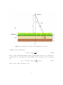
In order to describe the activity contribution more realistically, the whole radioactivity containing volume can be divided in several sub-volumes [7]. Each sub-volume, or
slab, has individual thickness, di , uniformly distributed radioactivity and consists of a
fraction of the total activity, see Figure 2.1.
According to Equation 2.5, the fluence rate from an infinitesimal volume is
dϕv =
Av p(E)C(E)
dV.
4πR2
(2.6)
where Av is the activity per unit volume and dV = rdrdφdz with φ as the azimuthal
angle. When integrating over the azimuthal angle a factor 2π is introduced and the
equation above becomes
Av r
dϕv =
p(E)C(E)drdz.
(2.7)
2R2
The photon fluence rate, which depends on the photon incidence angle, can be determined by setting r = Htanθ and dr = H(cosθ)−2 dθ. Then the following equation is
obtained:
Av tanθ
dϕv =
p(E)C(E)dθdz.
(2.8)
2
By rearranging Equation 2.1 the factor C(E) in Equation 2.8 is obtained
C(E) =
I0
= exp(−µr).
I
(2.9)
Because this factor is also depending on the material which the photon is passing through
and the vertical distance between the detector and the source, hence in this report the
5
Figure 2.1: A schematic description of the arrangement of the slabs.
attenuation factor is written as
µj d
Cj (d) = exp −
cosθ
(2.10)
where j is the current material and d is the vertical distance in m. If one considers the
vegetation as one of the slabs, the total attenuation factor from slab i can be expressed
as:
i−1
Y
Ctot,i = Cair (H − d1 )Cj,i (ui )
Cj,n (dn )
(2.11)
n=1
where j can be either vegetation or soil.
6
Photon Attenuation
A general description of the mass attenuation coefficient for soil, µsoil with unit m−1 ,
was developed earlier [8].
µsoil
(E) = 1.26 · 105 E −4−27 + 0.142E −0.445 − 2 · 10−5 ,
ρsoil
(2.12)
where the soil density ρsoil is given in kg/m3 and the energy E in MeV. This description
is valid for most types of soil and gives good results for photon energy within the range
0.3 to 3 MeV.
In order to approximate the attenuation coefficient for the vegetation, one can use a
linear combination between the attenuation of air and the attenuation of water [3]. Consider a vegetation height of hv in m and the mass per unit area of mv kg/m2 . Further
assume that the density of the vegetation is ρH2 O when compressed. Then the attenuation coefficient can be expressed as
mv
mv
µveg = 1 −
µair +
µH O .
(2.13)
hv ρH2 O
hv ρH2 O 2
The observed values for linear attenuation coefficient for water and air, µH2 O and µair
respectively, can be found in the NIST database [4]. The following equation was obtained
after plotting values in log-log scale and then a curve-fitting was applied. For photon
energy E in MeV the µH2 O is
µH2 O (E) = 100exp(−0.04(lnE)2 − 0.48lnE − 2.65)
(2.14)
The µair is described as Equation 2.15, taken from Boson et al.[7].
µair (E) = ρair 0.0623E −0.4754
(2.15)
These µs are given in m−1 and ρair in kg/m3 . The air density is assume to be a function
depending on three parameters [9], the air pressure P given in kPa, the temperature T
in ◦ C and the relative humidity h in %,
a = 3.348444
aP − (bT − c)h
,
parameters
(2.16)
ρair =
b = 2.52 · 10−5
T + 273.16
c = 2.0582 · 10−4 .
To summarize, the photon fluence contribution from slab i with thickness di can then
be expressed as
ZZ
Av p(E)
Ctot,i tan θdui dθ
(2.17)
ϕi =
2
with integration intervals
(
0 ≤ ui ≤ di
0 ≤ θ ≤ π/2.
7
(2.18)
2.2.2
Multiple Slabs Model
The activity in each slab can be written in terms of total activity per unit area, As . The
relation between the surface activity and the volume activity is
Av,i =
As k i
,
di
(2.19)
where di is the thickness of slab i and ki is a proportional factor that describes the
relative activity content in slab i. For total N slabs, the factor ki can be expressed as
Av,i di
ki = PN
.
A
d
v,j
j
j
(2.20)
Then according to Equation 2.17 the calibration factor for the multiple slab model is
N
Ṅ
ϕ
p(E) X ki
= εdet (E, θ)
=
As
As
2
di
ZZ
εdet (E, θ)Ctot,i tan θdui dθ.
(2.21)
i
2.2.3
Surface Deposition Model
The radionuclides will initially after a deposition be deposited on the surface. In this
model, assumption of uniformly distributed radionuclides on a perfectly flat surface is
made. This is an ideal model because in reality, the radionuclides transported by the
atmospheric process will not be distributed uniformly on the surface. To determine the
calibration factor for a such model, take N = 1 in equation 2.21 and assume simply that
the soil slab is extremely thin. The vegetation above the ground surface can be assumed
to be one of the slabs in multiple slab model. In such cases take N = 2 in order to take
the vegetation into account.
2.2.4
Volume Deposition Model
The radioactivity distribution may also be considered as uniform in the soil. Therefore
the calibration factor for such a model can be obtained by taking N = 1 in equation
2.21. If the vegetation above the ground surface is desired to be included, take instead
N = 2.
However, soon after a radioactive fallout, radionucides may penetrate a bit into the
ground. In order to get a quick result of the calibration factor for a so-called emergency
preparedness model [10], values in table 2.1 are assumed.
8
Table 2.1: Values used in calibration factor calculation for the emergency preparedness
model. Ingnore the last three values and set the relative activity content in the soil to 100%
if there is no vegetation.
Value
Parameter
Soil layer thickness
Soil density
[m]
0.02
[kg/m3 ]
500
Relative activity content
[%]
70
Vegetation height
[m]
0.1
[kg/m2 ]
0.5
[%]
30
Surface mass
Relative activity content
2.2.5
Exponential Model
Another model that may be applied in in-situ gamma-ray spectrometry is when the
concentration of radionuclides can be assumed to decrease exponentially with depth [5]:
A(z) = A0 e−αz ,
(2.22)
where A0 is the activity on the ground surface in unit Bq/m3 and α the reciprocal of
the relaxation length of unit m−1 for the radioactivity in the soil.
It is convenient to make a projection of the total activity in the soil on the surface
by integration of equation 2.22 from 0 to ∞ which gives Aa = A0 /α. Insert equation
2.22 in equation 2.6 and set again r = (H + z) tan θ. The fluence rate is then obtained,
1
dϕ = p(E)αAa e−αz tan θC(E)dθdz.
(2.23)
2
The attenuation factor above the ground is determined by an equivalent attenuation
coefficient
mv
mv
µeq = 1 −
µair +
µH O
(2.24)
HρH2 O
HρH2 O 2
and the fluence rate can be rewritten as
p(E)αAa
αcosθ + µsoil
dϕ =
Ceq (H)exp −
z tan θdθdz.
(2.25)
2
cos θ
Integrating z from 0 to ∞, the previous equation becomes
dϕ =
p(E)αAa sin θ
Ceq (H)dθ
2(α cos θ + µsoil )
and finally the calibration factor for the exponential model is
Z π/2
Ṅ
p(E) sin θ
=
εdet (E, θ)Ceq (H)dθ.
Aa
2(cos θ + µsoil /α)
0
9
(2.26)
(2.27)
2.3
Statistics and Data Analysis
First of all, two important statistical quantities are defined. For total N samples, the
sample mean and the sample variance are
N
1 X
x̄ =
xi
N
(2.28)
i=1
and
N
σ2 =
1 X
(xi − x̄)2 .
N −1
(2.29)
i=1
In many measurements, the measurand is not measured directly, but is expressed as a
function of other measurement quantities. In practice, a measurement result is only an
estimate of the value of the measurand. Therefore, the uncertainty of that estimate must
be included to give a complete measurement result [11]. Assume that the measurand Y
can be written as a function of measurement quantities X1 , X2 , . . . , XN ,
Y = f (X1 , X2 , . . . , XN ).
(2.30)
After N identical measurements, the estimate of Y can be taken as the mean of Y
n
y = Ȳ =
1X
Yk .
n
(2.31)
k=1
Further, assume that every input estimate of measurement quantity Xi consists of a
standard uncertainty u(xi ). This uncertainty can be of Type A, which is obtained by
the statistical analysis of series of observations, and Type B, which is obtained by other
methods than the statistical analysis of series of observations [11]. The combined uncertainty associated with Y , uc (y), can be determined analytically as shown in Equation
2.32 [11]. This combined uncertainty will give a perception about the quality of the
measurement result of Y .
N X
∂f 2 2
2
uc (y) =
u (xi ).
(2.32)
∂xi
i=1
However, the function f is not always differentiable. In case of a complex relation
between the input quantity and the measurand, a numerical approach may be convenient
[12]. For input quantities X1 , X2 , . . . , XN that are characterized by specific probability
density functions (PDFs), the output will get a certain probability distribution. Then
the combined uncertainty uc (y) is simply the standard deviation of the outputs. A useful
numerical method for the propagation of distributions is Monte Carlo methods [12].
2.3.1
Monte Carlo Method
Monte Carlo (MC) methods are a selection of methods that uses random samplings to
solve problems [13, 12, 14]. Samples from predetermined PDFs are used in simulations
10
to obtain the probability distribution and other statistical properties of an unknown
quantity. It is an old idea, scientists tried to determine the value of π using this idea
centuries ago [13]. Nowadays, the MC methods are widely used within many scientific
areas, e.g. physical science, engineering and finance. When using the MC method, one
must deal with the precision and the accuracy of the simulation results.
The MC method works as follow. M values of quantities Xi , i = 1...N , are selected
randomly from their PDFs, pxi . Using these M values for each input quantity, an output set Yk , k = 1, ..., M , is obtained. This process can be seen as a repetition of the
same experiment many times. Out of these Yk s, the estimates of Yk and its standard
deviation s can be determined using Equation 2.33 respective 2.34.
Ȳk =
s2 =
M
M
1 X
1 X
Yk =
f (X1,k , X2,k , ..., XN,k )
M
M
(2.33)
1
M
(2.34)
k=1
M
X
k=1
(Yk − Ȳk )2 .
k=1
Due to this random sampling, the parameter values with low occurrence probability
might be excluded from the input set if M is not large enough. Therefore, a large
number of samples must be drawn to ensure that the input sets are representative for
the parameter distributions and in turn avoid clusters in the output set. A large number
of samples requires large computer memory and also means a long calculation time.
However, these problems can be reduced by using a stratified sampling method [15], e.g.
Latin Hypercube sampling.
2.3.2
Latin Hypercube Sampling
The Latin Hypercube Sampling (LHS) method is a special stratified sampling method
that was developed by McKay et al. in 1979 [15]. Assume that the PDF for input
quantity xi is
Z
∞
pxi (ξ) =
gxi (ξ)dξ = 1.
(2.35)
0
The PDF for each input quantity is divided into M disjoint intervals, i.e. stratifications,
so that
Z
pxi (ξ) =
gxi (ξ)dξ,
k = 1, ..., M,
(2.36)
Ik
is equal for each interval Ik . Within every interval Ik one and only one sample is drawn
randomly. By doing this, M samples are taken for each input quantity. The order of
samples for each input quantity is shuffled randomly. Then the samples for each input
quantity are randomly paired to form M input sets which in turn give an output set
Yk , k = 1, ..., M . The outputs can then be analysed as in the case of using MC method.
The LHS method has several benefits compared to the MC methods. Using LHS, the
11
samples with low probability are forced to be represented in the input set. In this way,
clusters in the output set are avoided even if a small number of calculations is performed.
Earlier study has shown that it requires about 1/3 as many Latin Hypercube iterations
as MC iterations to get equal results [16].
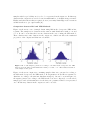
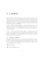
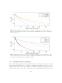
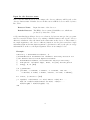
Comparison between MC and LHS Methods
Figure 2.2 shows two sets of sample drawn using MC method respective LHS in histograms. The samples were drawn from the same normal distribution with µ = 0 and
σ = 1. It can be seen that there is some clusters in the case of using the MC method.
These clusters may cause clusters in the output set, which can affect the statistical
properties of the outputs and that is not desirable.
Figure 2.2: 1 500 samples generated according to the MC method respective the LHS
method, from the same normal distribution with µ = 0 and σ = 1. The standard deviation
of the sample is also given.
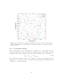
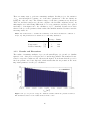
Figure 2.3 shows two input sets containing samples that were generated according to
the MC method respective the LHS method. Both parameter A and B were assumed to
distribute according to the uniform distribution U(0, 1). As can be seen in Figure 2.3,
the inputs generated according to the LHS method are more dispersed over the whole
sample space and each stratification for the these two parameters had been represented
once. In this way, clusters in the output set can be avoided.
12
Figure 2.3: Two input sets containing 70 samples generated according to the MC method
respective the LHS method. Both parameter A and B were assumed to distribute uniformly
between 0 and 1.
2.3.3
Uncertainty Analysis
The total uncertainty of the calibration factor consists of two components: the combined uncertainty of the detector efficiency calculation and the uncertainty from the
calculations. According to Equation 2.32, the total uncertainty can be determined by
u2total = u2detector + u2calculation .
(2.37)
The combined uncertainty of the detector efficiency is a Type B uncertainty and was
calculated to be 4% [6]. In order to determine the uncertainty from calculations, the
following two concepts are useful.
13
Law of Large Numbers [17]
The Law of Large Numbers (LLN) is a mathematical formulation which states
that the sample mean of random variables Xi will converge towards the expectation value as the number of samples increases, i.e.
n
1X
µ = E[Xn ] = X̄n = lim
Xi
n→∞ n
(2.38)
i=1
Consider that the PDF for every input quantity is stratified in N intervals, then N
calibration factors (CF) will be obtained after calculations. According to the LLN, the
estimate of the CF will converge towards the expectation value of the CF when N → ∞.
Also, the estimation of the uncertainty of the CF will converge towards the standard
deviation of the CF. The relative uncertainty associated with calculations described in
Equation 2.37 can be determined by the ratio between the standard deviation of the CF
and the expectation value of the CF, i.e.
ucalculation = S̄N /ȲN .
14
(2.39)
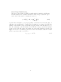
3
Method
Initially, a simple sensitivity analysis was performed for the linear attenuation coefficient of air in order to reduce the amount of input quantities if possible. Models for
the calibration factor calculation with different deposition types were implemented in
MatLab (version R2014b) together with other necessary functions. The models were
then modified to be able to be used for different purposes. Some user-friendly graphical
user interfaces (GUIs) were build using a build-in interactive GUI construction kit, the
GUI development environment (GUIDE).
To generate sample sets using the LHS method, build-in MatLab functions were used
with some modifications. By assuming independence between all parameters, the covariances could be set to zero. The samples were generated as vectors, except for the
soil condition parameters, e.g. the thickness and the density, where the samples were
generated as matrices.
In order to be able to use LLN and CLT, the number of calculations must be large
enough. So several tests were done in order to investigate how the relative uncertainty
associated with calculations varies with the number of calculations. Also how the relation between the number of iterations and the number of calculations per iteration
affects the uncertainties was investigated.
3.1
Sensitivity Analysis
Sensitivity analysis is performed in order to identify the most important ones among a
large number of input parameters. In this project, how the linear attenuation coefficient
of air, µair , was affected by its input parameters was examined. µair is a function of the
photon energy and is proportional to the air density, see Equation 2.15. The air density
is in turn depending on three parameters:
the air pressure
the air temperature
the relative humidity in the air
15
There are many ways to perform a sensitivity analysis. In this project, the variation
of µair was investigated by fixing one of the three parameters of the air density an
letting the other two vary. The variation range for the three parameters are shown in
Table 3.1, and these ranges were chosen to adjust to the Swedish conditions [18, 19]. 10
000 samples were taken using LHS method for every parameter and they were paired
randomly to form input sets to the calculation of µair . Standard deviation were then
taken for the µair s, the parameter that resulted the smallest standard deviation was the
most important one.
Table 3.1: Values used to examine the sensitivity of the linear attenuation coefficient of
air [18, 19]. All parameters were assumed to be uniformly distributed.
3.1.1
Average
Limits
Pressure
[kPa]
100
±10
Temperature
[◦ C]
5
±20
Relative humidity
[%]
80
±20
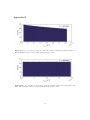
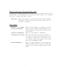
Results and Discussions
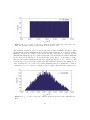
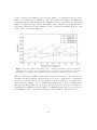
The results of sensitivity analysis of µair are shown in Figure 3.1, 3.2 and 3.3. Similar
figures for two other photon energies can be found in Appendix B. The standard deviations for respective results are also shown in the figures. It is shown that the µair s for
fixed air pressure were least dispersed, which means that the air pressure is the most
important parameter for the µair calculation.
Figure 3.1: µair for photon energy E = 100 keV calculated when the pressure was fixed.
The standard deviation of the results is shown in the corner.
16
Figure 3.2: µair for photon energy E = 100 keV calculated when the temperature was
fixed. The standard deviation of the results is shown in the corner.
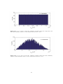
The standard deviation of µair is largest when the relative humidity was fixed. This
means that the relative humidity is the least important parameter. Note that the relative
humidity describes the relation between the amount of moisture (or water) and the
maximal amount in the air at a certain temperature [19], the higher the relative humidity
is, the more moist the air is. It is known that water has good attenuation ability,
therefore the relative humidity should have significant impact on µair . However, this
relation can not be seen in the results from this sensitivity analysis. One might use an
other description for µair where the relative humidity has more significance. A linear
combination of µair,dry and µwater might be used, compare this idea with equation 2.15.
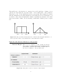
Figure 3.3: µair for photon energy E = 100 keV calculated when the relative humidity was
fixed.
17
However, when determining µair using equation 2.15, it results in that the relative humidity is not a significant parameter. This means that it has a small contribution to the
uncertainty for calculation of the µair , in turn the calculation of the calibration factor.
Therefore the relative humidity will be designed to be an un-sampled parameter in the
calibration calculation program.
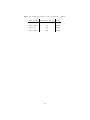
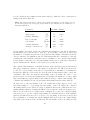
Parameters that contribute to the combined uncertainty are shown in table 3.2. By
assuming independence between all parameters, their individual contributions to the
uncertainty can be determined. Set uncertainties of other parameters to zero, the deviation of the results will then only come from the parameter in question.
Table 3.2: table showing whether the parameter √
is contributing or not to the uncertainty
of the calibration factor for different models. The indicates ”Yes” and × ”No”.
Parameters
Detector height
Air pressure
Air temperature
Vegetation height
Surface mass
Activity content in veg.
Surface
√
Volume
√
Multiple slabs
√
Exponential
√
√
√
√
√
√
√
√
√
√
√
√
√
√
√
√
√
√
√
√
√
√
√
√
√
√
Soil slab thickness
×
Soil density
×
√
Activity content in soil
3.2
Models
×
×
√
×
Accuracy Investigation
As described in section 2.3.3, the relative uncertainty associated with the calculations
can be obtained by using Equation 2.39. However, the estimate of the uncertainty is
depending on how many calculations that are performed. The more calculations that
are performed, the better estimation of the uncertainty. Therefore in the calibration
software, there has to be a compromise between time and accuracy.
According to the LLN, both the number of iterations and the number of calculations
per iteration should be large. However, it is not realistic to spend too long time to
perform CF determination calculation for in-situ spectrometry measurements. Different
combination of simulations and calculations per simulation was investigated for energies
E = {100, 779, 1048} keV in order to get an idea about how the relative uncertainty in
the uncertainty associated with the calculation of the CF varies with different combina18
tions.
The investigation was performed using the emergency preparedness model with inputs
according to table 3.3. All parameter values were assumed to be uniformly distributed.
For definition of the half-width of limit, see figure 3.4.
Table 3.3: Values used in the accuracy investigation. All parameter values were assumed
to be uniformly distributed.
Parameter
Medium
Half-width of limits
[kPa]
100
±5
[◦ C]
20
±10
Relative humidity
[%]
80
0
Detector distance to the ground
[m]
1
±0.05
Veg. height
[m]
0
–
[kg/m2 ]
0
–
[%]
0
–
[kg/m3 ]
900
±800
Soil slab thickness
[m]
0.03
±0.02
Activity content in soil
[%]
100
±0
Pressure
Temperature
Surface mass
Activity content in veg.
Soil density
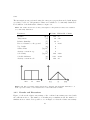
Figure 3.4: The probability density functions for uniform and triangular distribution. m
is the expectation value or the medium and a is the half-width of limits.
3.2.1
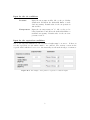
Results and Discussions
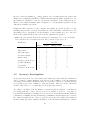
Figure 3.5 shows the relative uncertainty of the combined uncertainty associated with
the calibration factor. The number of calculations per simulation and the number of
simulations were varied. It is possible to see in Figure 3.5 that the relative uncertainty
19
of the combined uncertainty is lower for large number of calculations and also larger
number of calculations per simulation. Also, the relative uncertainties for simulations
containing 100 and 120 calculations per simulation did not vary much. For increasing
number of simulations, the relative uncertainty of the combined uncertainty should be
decreasing, which means better estimation of the combined uncertainty. However, such
trend could not be seen in Figure 3.5.
Figure 3.5: The relative uncertainty of the combined uncertainty associated with the
calibration factor based on the preparedness model and the photon energy E = 100 keV.
The number of calculations per simulation and the number of simulations were varied.
Tabel 3.4 shows the calculation time and the standard deviation of the standard uncertainty associated with the calibration factor for some combinations of calculations.
As can be seen in the Table 3.4, the standard deviation would not necessarily be reduced when the number of total calculations was increased, but the calculation time
was increased much. Therefore, it is up to the user to decide about the the number of
calculations per simulation and the number of simulations and thereby the accuracy of
the estimation of the combined uncertainty associated with the calibration factor.
20
Table 3.4: Calculation results for photon energy E = 100 keV.
Cal. × Sim.
Calculation time [s]
S. D.
100 × 50
275
0.0443
100 × 100
550
0.0414
120 × 50
330
0.0368
120 × 100
660
0.0409
21
4
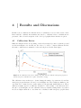
Results and Discussions
In this section, results from calibration factor calculation, detector field-of-view calculation and the combined uncertainties associated to calibration factor calculations are
presented. Also a brief description of the developed graphical user interface is given.
4.1
Calibration Factor
Different calibration factors depending on the radioactivity deposition on/in the ground
are shown in Figure 4.1, 4.2 and 4.3. In order to be able to compare different models,
the same conditions were assumed for the models plotted in the same figure.
Figure 4.1: Calibration factors for surface deposition model and the emergency preparedness model plotted as function of photon incidence energy.
The calibration factors that were obtained using the surface deposition model and the
emergency preparedness model can be seen in Figure 4.1. The results are similar to the
ones that were obtained from a earlier study [6], though with small differences. These
differences might depend on different description of the density of air that was used.
As can be seen in Figure 4.1, the calibration factors calculated using surface deposition
model are higher than those ones that were calculated with emergency preparedness
22
model. This is due to the fact that no attenuation in soil occurs in the surface deposition model.
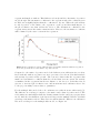
In Figure 4.2 the calibration factors for exponential respective multiple slab model are
shown for the case where the same detector might have been used. In order to obtain a
description of how the radioactivity penetrates into the soil, empirical values [7] for activity contents were used. An exponential function was adapted to the empirical values
so that the activity in the soil can be described in the form as in Equation 2.22. The
data and the adaption of the data points is shown in Figure C.1, which can be found in
Appendix C.
Figure 4.2: Calibration factors for multiple slabs model and the exponential model plotted
as function of photon incidence energy. The relaxation length was adapted to empirical data
from Boson et al. [7].
From Figure 4.2 one can see that the curves have similar shape, which is expected. For
the same conditions, the exponential model gives higher calibration factors, about 30%
more than calibration factors calculated using multiple slab model. It is because that
there had been an overestimation of the activity near the ground surface in the data
adaption. And in combination of low attenuation, the photon fluence rate for the exponential model might be overestimated and in turn the calibration factor. However, it is
difficult to say how realistic the exponential model is due to the lack of empirical data
of the calibration factors. The calibration factor calculated using the exponential model
will vary depending on the exponential function that was adapted to the data points
and also the soil density that was assumed. Since soil has a good attenuating ability,
by assuming homogeneous soil density in depth will result an incorrect estimation of the
photon fluence rate and thereby the calibration factor. This problem can be reduced by
using relaxation mass depth instead of relaxation length [2].
23
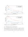
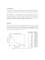
The calibration factors for exponential model with several relaxation lengths are shown
in Figure 4.3. Note that the surface deposition model can also be described as en exponential model with zero relaxation length. The calibration factors are decreasing with
increasing relaxation lengths. The greater the relaxation length is, the deeper the radionuclides penetrate into the soil [5]. When the radionuclides penetrate deeper in the
soil, it means that the possibility for them to be detected is lower because the attenuation
of the soil. Therefore, the calibration factors are low for long relaxation lengths.
Figure 4.3: Calibration factors for the exponential model with varying radionuclide relaxation lengths plotted as function of photon incidence energy. The soil density was set to
1500 kg/m3 and the activity on the ground surface was constant.
4.1.1
The Effects from Vegetation
Figure 4.4, 4.5 and 4.6 present the calibration factors calculated in the presence of
radioactivity in the vegetation. The vegetation conditions were set to the same for all
deposition models and the values are presented in Table 4.1.
Table 4.1: Values of vegetation condition used in the calculation of calibration factor in
presence of vegetation.
Parameter
Value
Height
Surface mass
[m]
0.1
[kg/m2 ]
1
[%]
30
Activity content
The calibration factors are always higher for calculation with radioactivity containing
24
vegetations than those without. This difference is barely visible for the surface deposition
model, though. The attenuation coefficient for the vegetation under the conditions given
in Table 4.1 is slightly higher than the coefficient for dry air. When the radioactivity
is only deposited on the surface, the vegetation on the ground has small impact on
the photon fluence rate that reaches the detector. The attenuation coefficient for the
vegetation increases if the surface mass increases. However, the attenuation coefficient
will be limited by the water content in the vegetation.
Figure 4.4: Comparison between calibration factors calculated with and without vegetation
above the ground based on the surface deposition model.
Compared to the surface deposition model, the differences in calibration factors calculated with and without vegetation are more pronounced for the models which include
radioactivity deposition in the ground. The reason for this is that the vegetation has
much lower attenuation coefficient than the soil and that, in some extent, the activity
accumulated in the vegetation has shorter distance to the detector. Both these factors
give rise to increased photon fluence rate, and in turn increased calibration factor due
to the proportionality between these to quantities.
For the multiple slabs model, the soil conditions were taken from an earlier study [7].
The difference is even larger compare to the surface and volume deposition model. The
soil densities are much higher than the density assumed in the emergency preparedness
model. And also the thickness of the layers are larger in the multiple slabs model which
gives larger attenuation effects. These factors result in that the difference in calibration
factors is even larger for the multiple slabs model, see Figure 4.6.
25
Figure 4.5: Comparison between calibration factors calculated with and without vegetation
above the ground based on the emergency preparedness model.
Figure 4.6: Comparison between calibration factors calculated with and without vegetation
above the ground based on the multiple slabs model.
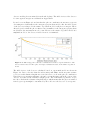
4.2
The Field-of-View of the Detector
Figure 4.7, 4.8 and 4.9 present the detector’s field-of-view for several photon energies
when assuming different deposition model. In these figures the contribution of full-energy
peak count rate from remote region was plotted as a function of the field-of-view of the
detector. The full-energy peak count rate contribution from remote region was defined
as the ratio between the photons emitted from remote region that are registered by the
26
detector and the photons emitted from the whole plane. The field-of-view of the detector
for some typical energies are tabulated in Appendix D.
It can be seen in Figure 4.7 and 4.8 that the photon contribution from remote region is
decreasing more drastically for the emergency preparedness model. Also the field-of-view
of the detector is larger for the surface deposition model for all photon energies. These
effects depend on that the photon fluence rate is smaller for the emergency preparedness
model where the attenuation in soil occurs. However, the surface deposition model is a
simplified model, so the detector field-of-view is overestimated.
Figure 4.7: Full-energy peak count rate contribution from remote region as function of the
detector field-of-view for three photon energies. Calculation based on the surface deposition
model.
The field-of-view of the detector calculated based on exponential model are shown in
Figure 4.9. Due to the fact that the radioactivity will diffuse and homogenise as time
goes by, several relaxation lengths were tested in order to see how the photon contribution
from remote regions varies with time. As can be seen in the figure, the field-of-view of the
detector decreases as the relaxation length grows. The radionuclides penetrate deeper
into the soil when the relaxation length is larger, which means that the photons emitted
from deeper regions might be attenuated by the soil before the detector does response.
27
Figure 4.8: Full-energy peak count rate contribution from remote region as function of
the detector field-of-view for three photon energies. Calculation based on the emergency
preparedness model.
Figure 4.9: Full-energy peak count rate contribution from remote region as function of the
detector field-of-view for photon energy E = 660 keV. Calculation based on the exponential
model with four different photon relaxation lengths.
4.3
Combined Uncertainties
The combined uncertainties are shown in Table E.1, E.2 and E.3, which can be found
tables in Appendix E. In order to obtain the combined uncertainty associated to the calculation based on the surface deposition model and the emergency preparedness model,
values in Table 4.2 were used. For calculation based on the multiple slabs model, values
28
for soil conditions were taking from an earlier study [7], while the other conditions were
taking as shown in Table 4.2.
Table 4.2: Values used in the combined uncertainty investigation for the surface deposition model respective the emergency preparedness model. Parameters were assumed to be
uniformly distributed.
Parameter
Medium
Limits
Pressure
[kPa]
100
±5
Temperature
[◦ C]
7.5
±22.5
Relative humidity
[%]
80
0
Detector height
[m]
1
±0.05
[kg/m3 ]
900
±800
Soil slab thickness
[m]
0.03
±0.02
Activity content in soil
[%]
100
0
Soil density
For the surface deposition model, the combined uncertainties for the whole calibration
measurement were between 4.2% to 4.9% (k = 1), depending of the photon energy and
the number of calculations performed. Note that the uncertainty contribution from the
detector efficiency determination was 4%. This means that the contribution of the uncertainty associated with the calibration factor calculation to the combined uncertainty
is very small, because there are only uncertainties in the detector efficiency calibration,
the air density and the distance between the detector and the source.
The combined uncertainties for calculations based on the emergency preparedness model
have larger variations compare to the surface deposition model. They vary from 27%
to 37% (k = 1) depending on the photon energy and the total number of calculations.
Because the difference between the two models is the soil attenuation, these ”extra” uncertainties could only come from the uncertainty of the soil density. In order to cover
the most types of soil, the uncertainty in the soil density was assumed to be large. This
large uncertainty propagates further and results in a large combined uncertainty. The
combined uncertainties are also in agreement with results from an earlier study [6].
As stated above, the uncertainty of the soil density has a large impact on the combined uncertainty, i.e. by lowering the uncertainty of the soil density the combined
uncertainty will decrease. There is a lack of empirical data for the calibration factor assuming multiple slabs model using the HPGe detector that is considered in this project.
But if one uses the detector characterised by Equation 2.3 and soil conditions taking
from Boson et al. [7], the combined uncertainty for calculations based on the multiple
slabs model will vary from 5.2% to 6.2% (k = 1) depending on the photon energy and
the total number of calculations. In the multiple slabs model, the soil column sample
was divided in several sections. In this way, the uncertainty of the soil density in each
29
section can be lowered. Due to the lowered uncertainties, the combined uncertainty for
the multiple slabs model is much lower compare to the emergency preparedness model
even though there are more input quantities that are associated with uncertainties.
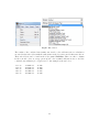
4.4
Graphical User Interface
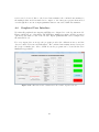
User-friendly graphical user interfaces(GUIs) were designed for each deposition model.
Figure 4.10 shows one of the GUIs. The GUIs have similar appearance and the execution
options are the same for all of the models. Input quantities that can be sampled are
shown in Table 3.2.
For every input photon energy, the program provides the calibration factor and the
detector’s field-of-view in external figures. The combined uncertainty is saved as a text
file (.txt) for further use. More details about the program can be found in the User
Manual in appendix F.
Figure 4.10: The GUI for the calculation for the volume deposition model.
30
5
Conclusions
The designed software calculated the calibration factor well for the surface deposition
model and the emergency preparedness model. Validation of the calibration factor must
be performed for the multiple slabs model and the exponential model. The results of the
effect of the vegetation and the field-of-view of the detector were reasonable, although
validation need to be performed.
The combined measurement uncertainty based on the surface deposition model was calculated to be between 4.2% to 4.9% (k = 1), depending on the photon energy. For
the emergency preparedness model, the total measurement uncertainty was in the range
27% to 37% (k = 1), depending on the photon energy. The high uncertainty in the
soil density estimation contributed to a high combined measurement uncertainty when
the calculation performed was based on the emergency preparedness model. This high
uncertainty is due to the fact that the density assumed in the emergency preparedness
model should cover many ground types. If the density is measured for soil samples, the
uncertainty of the density will be reduced significantly resulting in a decreased combined
measurement uncertainty for the emergency preparedness model. The combined uncertainty for the multiple slabs model and the exponential needs to be validated.
31
6
Further Work
Due to the lack of empirical data during the time of this project, some quantities should
be validated in the future. They are:
the calibration factor and its combined uncertainty based on the multiple slabs
model and the exponential model
the calibration factor for models that include vegetations on the ground
the field-of-view of the detector for all models
Also, some improvements should be done for a more user-friendly software, such as
functions that can handle incorrect inputs.
32
References
[1] G. Choppin, J. O. Liljenzin, and J. Rydberg. Radiochemistry and Nuclear Chemistry. Third Edition. Butterworth-Heinemann.
[2] ICRU. Gamma-ray spectrometry in the environment, icru report 53. Technical
report, International Commission on Radiation Units and Measurements. 1994.
[3] J. P. Laedermann, F. Byrde, and C. Murith. In-situ gamma-ray spectrometry:
the influence of topography on the accuracy of activity determination. Journal of
Environmental Radioactivity, 38(1):1–16, 1998.
[4] J. H. Hubbell and S. M. Seltzer. X-ray attenuation and absorption for materials
of dosimetric interest. Technical report, The National Institute of Standard and
Technology (NIST). Available from http://www.nist.gov/pml/data/xraycoef/.
[5] H. J. Beck, J. DeCampo, and C. Gogolak. In-situ Ge(Li) and NaI(Tl) gammaray spectrometry. HASL-258, Health and Safety Laboratory, US Atomic Energy
Commission.
[6] J. Boson, H. Ramebäck, T. Nylén, and K. Lidström. Kalibrering av en HPGedetector för gammaspektrometri i fält. FOI-R–2914–SE, FOI, Umeå, Sweden. 2010.
[7] J. Boson, K. Lidström, T. Nylén, G. Ågren, and L. Johansson. In-situ gamma-ray
spectrometry for environmental monitoring: A semi empirical calibration method.
Radiation Protection Dosimetry.
[8] W. Sowa, E. Martini, K. Gehreke, P. Marschner, and M. J. Naziry. Uncertainty of in
situ gamma ray spectrometry for environmental monitoring. Radiation Protection
Dosimetry, 27(2):93–101, 1989.
[9] G. Sibbens and T. Altzitzoglou. Preparation of radioactive sources for radionuclide
metrology. Metrologia, 44(1):71–79, 2007.
[10] K. Lidström and T. Nylén. Beredskapsmetoder för mätning av radioaktivt nedfall.
FOA-R–98-00956-861–SE, FOA, Umeå, Sweden. 1998.
[11] Joint Committee for Guides in Metrology(JCGM). The guide to the expression of
uncertainty in measurement(GUM). Available from http://www.bipm.org/utils/
common/documents/jcgm/JCGM_100_2008_E.pdf.
33
[12] Joint Committee for Guides in Metrology(JCGM). Evaluation of measurement data
– supplement 1 to the ”guide to the expression of uncertainty in measurement” –
propagation of distributions using a monte carlo method. Available from http:
//www.bipm.org/en/publications/guides/gum.html.
[13] W. L. Dunn and J. K. Shultis. Exploring Monte Carlo Method. Elsevier.
[14] K. Jareteg. Monte carlo simulations. Available from http://klas.nephy.
chalmers.se/teaching/montecarlo2013/documents/Slides.pdf. Lecture Handout, 2013.
[15] M. D. McKay, R. J. Beckman, and W. J. Conover. A comparison of three methods
for selecting values of input variables in the analysis of output from a computer
code. Technometrics.
[16] Palisade. Latin Hypercube vs. Monte Carlo. Available from http://www.palisade.
com/downloads/help/risk35/faq_html/latinhypercubevs.montecarlo.htm.
[10 Oktober 2014].
[17] J. A. Rice. Mathematical Statistics and Data Analysis. Third Edition. Thomson
Higher Education.
[18] Swedish Meteorological and Hydrological Institute. Lufttryck. Available from http:
//www.smhi.se/kunskapsbanken/meteorologi/lufttryck-1.657. [19 September
2014, written in Swedish].
[19] Swedish Meteorological and Hydrological Institute.
Luftfuktighet.
Available from http://www.smhi.se/kunskapsbanken/meteorologi/luftfuktighet1.3910. [19 September 2014, written in Swedish].
34
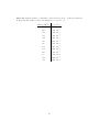
Appendix A
Table A.1: Values for parameters in Eq.(2.3) [6]. Six significant figures are retained for
further calculation. These parameters are valid for this particular detector, since different
detectors will have different energy response as well as angular response.
Parameter
Value
a1
33.9245
a2
-0.0392096
a3
0.0353600
a4
0.00132088
a5
-487.125
a6
-0.0671579
a7
8.10449
a8
0.215457
a9
6.83275
a10
-11.5236
a11
0.848338
35
Table A.2: Mass attenuation coefficients for water that were used to obtain the parameters
in Eq.(2.14). The density of water was assumed to be 1 g/cm3 . [4]
Energy [MeV]
µ/ρ[cm2 /g]
0.1
1.707 · 10−1
0.15
1.505 · 10−1
0.2
1.370 · 10−1
0.3
1.186 · 10−1
0.4
1.061 · 10−1
0.5
9.687 · 10−2
0.6
8.956 · 10−2
0.8
7.865 · 10−2
1.0
7.072 · 10−2
1.25
6.323 · 10−2
1.5
5.754 · 10−2
2.0
4.942 · 10−2
3.0
3.969 · 10−2
36
Appendix B
Figure B.1: µair for photon energy E = 661 keV calculated when the pressure was fixed.
The standard deviation of the results is shown in the corner.
Figure B.2: µair for photon energy E = 661 keV calculated when the temperature was
fixed. The standard deviation of the results is shown in the corner.
37
Figure B.3: µair for photon energy E = 661 keV calculated when the pressure was fixed.
The standard deviation of the results is shown in the corner.
Figure B.4: µair for photon energy E = 1048 keV calculated when the relative humidity
was fixed. The standard deviation of the results is shown in the corner.
38
Figure B.5: µair for photon energy E = 1048 keV calculated when the temperature was
fixed. The standard deviation of the results is shown in the corner.
Figure B.6: µair for photon energy E = 1048 keV calculated when the relative humidity
was fixed. The standard deviation of the results is shown in the corner.
39
Appendix C
Table C.1: Values from Boson et al., [7] that were used to obtain the inout data for the
exponential model.
Thickness
Density
Fraction of total
[cm]
[kg/m3 ]
activity [%]
1
2.0
1210
80
2
5.0
1460
16
3
9.4
1720
4
Slab
Figure C.1: Adaption of an exponential function to data points from Boson et al. [7].
Table C.2: Input values that were used in the exponential model for comparison between
the multiple slabs model and the exponential model.
Density [kg/m3 ]
1500
[Bq/m3 ]
500
A0
Relaxation length [m]
40
0.015
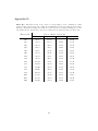
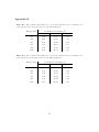
Appendix D
Table D.1: The field-of-view of the detector corresponding to 95% contribution of fullenergy peaks for all models. Soil conditions for multi-slab model were taken from an earlier
study [7]. Relaxation length was taken as 0.3 cm and the soil density 1500 kg/m3 for the
exponential model. Beside these, all other conditions were taken the same for all models.
Detector Field-of-View [m]
Energy [keV]
Surface dep.
Preparedness
Multi-slabs
Exponential
100
50.56
17.82
-
14.00
122
56.14
19.59
12.88
15.29
140
60.32
20.88
13.68
16.24
160
64.63
22.17
14.49
17.19
180
78.62
23.36
15.22
18.05
200
72.34
24.46
15.89
18.84
244
79.74
26.61
17.13
20.39
344
93.70
30.63
19.52
23.20
444
105.10
33.87
21.34
25.41
661
124.91
39.43
24.32
29.09
779
134.00
41.93
25.62
30.70
867
140.06
43.62
26.49
31.79
964
146.38
45.37
27.37
32.90
1086
153.76
47.40
28.38
34.18
1112
155.27
47.82
28.58
34.44
1408
170.90
52.14
30.70
37.12
41
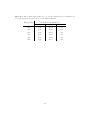
Appendix E
Table E.1: The combined uncertainty (k = 1) for the calibration factor calculation for
some typical photon energies, based on total 500 calculations.
Energy [keV]
Combined Uncertainty [%]
Surface dep.
Preparedness
Multi-slabs
122
4.46
37.45
6.23
344
4.14
32.16
5.68
661
4.28
29.29
5.41
779
4.27
28.62
5.35
964
4.27
27.78
5.28
1112
4.26
27.73
5.23
Table E.2: The combined uncertainty (k = 1) for the calibration factor calculation for
some typical photon energies, based on total 1000 calculations.
Energy [keV]
Combined Uncertainty [%]
Surface dep.
Preparedness
Multi-slabs
122
4.47
37.09
6.20
344
4.37
31.80
5.66
661
4.30
28.95
5.39
779
4.30
28.28
5.33
964
4.26
27.44
5.26
1112
4.25
26.90
5.21
42
Table E.3: The combined uncertainty (k = 1) for the calibration factor calculation for
some typical photon energies, based on total 2000 calculations.
Energy [keV]
Combined Uncertainty [%]
Surface dep.
Preparedness
Multi-slabs
122
4.45
36.64
6.17
344
4.34
31.40
5.64
661
4.28
28.58
5.38
779
4.27
27.92
5.32
964
4.25
27.09
5.24
1112
4.24
26.55
5.20
43
Appendix X
User Manual
Software for Calibration
in In-situ Gamma-Ray Spectrometry
This manual is aimed to give guidance for using the software for calibration of gammaray spectrometric in-situ measurements. MatLab, version R2012b or later, is required
to run this software since it was designed and comprises MatLab GUI.
The software is designed to be able to handle photons with energy up to 3 MeV, in
other words, it can be used for most relevant photon energies in environmental measurements. However, one limitation is the energy range for which the intrinsic calibration of
the HPGe detector was done for. For each input energy, the software has three outputs:
the detector field-of-view, the calibration factor and the combined standard uncertainty
for these measurands. The calibration factor is the total measurement efficiency which
is an important parameter when comes to activity determination on site.
For calculation of the combined standard uncertainties, the method Latin Hypercube
sampling is used. Parameters that contribute to the combined standard uncertainty can
be sampled from three continuous probability distributions. The results are then saved
in an external text file for further use.
Getting Started
Find the file main.m and open it in MatLab by a double click. Click on the icon run to
run the script/software. However, depending on the MatLab version, this icon will have
different appearance.
After you had started the software, a menu window appears. See Figure F.1 for how the
run button and the menu window appears in the MatLab version R2014b.
Figure F.1: The run icon and the main menu.
Menu
There are five option buttons in the menu window, four deposition model buttons and
one cancel button.
Models
Choose the desired model by clicking the corresponding button,
then a graphical user interface where you do the inputs for the
chosen deposition model is opened.
Cancel
You will receive a request, if answer ”Yes”, the software shuts down.
1
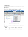
Graphical User Interface
One of the Graphical user interfaces (GUI) is shown in figure F.2. The interfaces have
different layout depending on the selected deposition model, but the differences are small.
The input boxes are arranged in panels in order to give you a better input overview.
There are already default values in some of the boxes, the calculations will be performed
using these values if you do not change them.
Figure F.2: User interface for a volume deposition model.
There are always five execution options, see the colored push buttons in figure F.2. Their
functions are described briefly below.
Plot Calibration Factors
An external window with plot of calibration factor versus photon energy is opened.
Do Uncertainty Analysis
Simulate the combined standard uncertainty for
each input energy.
Detector Field-of-View
An external window with a table showing the
detector field-of-view for corresponding energies
is opened.
Change Model
Back to the main menu for model change.
Exit
Exit the GUI and the software shuts down.
2
How to Enter Input Data
Follow the advice below in order to avoid any unsuccessful calculations. Figure F.3 show
the left part of a GUI.
Figure F.3: The left part of a GUI.
Input for the photon property
Energy
Input desired photon energies as a list separated by space or comma in
the unit [keV].
Defaults
Choose the preprogrammed photon energies by pressing the radio buttons. The default energies are: {100 122 140 160 180 200 244 344 444
661 779 867 964 1086 1112 1408} [keV]. These energies will be displayed
in the boxes under the input boxes for energy. Please do not change any
number in this box.
3
Input for the detector name
Due to the fact that all detectors are unique, the detector efficiency will depend on the
detector characteristic. Default detector in this case is a HPGe detector made by Ortec
Inc., USA.
Detector Name
Input the name of the detector.
Default Detector
The HPGe detector named defaultDetector, which was
produced by Ortec Inc., USA.
redJa, man kan lägga till nya detectorer, sedan är det bara att anropa den i programmet.You can add another detector by writing a MatLab function file for the detector
efficiency calculation. Give the function the same name as the detector. There must be
two input argument to the detector efficiency function, set the photon incidence angle
with unit radian as the first input argument to the function, and set the photon energy
with unit MeV as the second input argument. There is an example below.
Example:
function y = defaultDetector(theta, e)
% defaultDetector determines the intrinsic efficiency detector for
% the default detector from empirical studies
%
defaultDetector(Theta, E) returns the detector efficiency
%
with photon incidence angle, Theta, in [rad] and the photon
%
energy, E, in [MeV]
% A = parameters
A = [33.9245, -0.0392096, 0.0353600, -0.00132088, -487.125, ...
-0.0671579, 8.10449, 0.215457, 6.83275, -11.5236, 0.848338];
E = e*1000; % convert to [keV]
y = exp(A(1) + A(2)*theta.^2 + A(3).*theta + A(4).*E + ...
A(5)./E + A(6)*cos(A(7)*theta./E.^A(8) - A(9)) + ...
A(10)*log(E) + A(11)*(log(E)).^2);
end
4
Input for the name of the uncertainty result
Regarding the uncertainty analysis the result will be saved as a text file, and the desired
file name will be given in this panel. You can use any symbol when you do your input,
but please do remember the name of the file.
File Name
Input desired name for the file in where the uncertainty analysis
result is saved. If the name already exists, the content of the old
one will be overwritten.
Other inputs
Number of Calculations per Simulation
Enter the desired number of calculations per simulation. The probability density functions of every
input quantities are divided into the number that
is entered here.
Number of Simulation
Enter the desired number of simulations.
Contribution of Counts
Enter the desired field-of-view in percent. The detector field-of-view is defined as the radius of a circle where the contribution of counts from its area
is a certain percentage of the number of the counts
from a circle with infinite radius.
Relative Humidity
Enter the relative humidity for the air density calculation. Default value 80% can be used since this
parameter does not have a significant effect on the
result.
5
The middle part of the interface is constructed as a table with three columns. A general rule is to first input the expectation value, or the nominal value, of the parameter.
Thereafter you choose the distribution in the pop-up menus. The parameters can have
uniform, triangular and normal distributions. Depending the selected distribution, you
are asked to enter either the half-width of limits or standard uncertainties of the distribution in the third column. For the meaning of half-width of limits, please see figure
F.4.
Figure F.4: The probability density functions for uniform and triangular distribution. m
is the expectation value or the medium and a is the half-width of limits.
Input for the detector distance to the ground
Detector Height
Enter detector distance to the ground in meters.
Choose the probability distribution and fill in the halfwidth limits or standard uncertainty. Default value for
the detector distance to the ground is 1 m.
Figure F.5: The panel for detector and air condition inputs.
6
Input for the air conditions
Pressure
Input the air pressure in kPa. Choose the probability
distribution and fill in the half-width limits or standard uncertainty. Default value for the air pressure is
101.325 kPa.
Temperature
Input the air temperature in ◦ C. Choose the probability distribution and fill in the half-width limits or
standard uncertainty. Default value for the air temperature is 20 ◦ C.
Input for the vegetation conditions
Due to the algebraic limitations, the vegetation height must be non-zero. If there is
not any vegetation, set the surface mass to zero instead. The activity content in the
vegetation slab will then be set to zero automatically, as well as their ranges or variances.
Figure F.6: An example of the panel for vegetation condition inputs.
7
Height
Input the vegetation height in meters. Choose the
probability distribution and fill in the half-width limits or standard uncertainty. Default value for the vegetation height is 0.1 m.
Surface Mass
Input the surface mass in kg/m2 . Choose the probability distribution and fill in the half-width limits or
standard uncertainty. Set surface mass to 0 kg/m3 if
there is not any vegetation on the ground.
Activity Content
Input the activity content in Bq/m3 or proportion in
the vegetation slab. Choose the probability distribution and fill in the half-width limits or standard uncertainty. Set activity content to 0 % if there is not
any activity content in the vegetation on the ground.
Input for the soil conditions
The panels where you enter soil condition inputs have different appearance depending
on the selected deposition model. The default values will also be different. For the
surface deposition model, the soil slab thickness is infinite small and the soil density is
1000 kg/m3 . For the volume deposition model, the soil slab thickness is 0.02 m and the
soil density is 500 kg/m3 which are the values for calculation using emergency preparedness model.
For multiple slab model the soil condition must be specified for every slab. Enter the
values as a list separated by space or comma. When you fill in the number of slabs the
software will remind you how to enter the soil conditions.
Figure F.7: The panel for soil condition inputs for the volume deposition model.
8
Thickness
Enter the soil slab thickness in m. Choose the probability distribution and fill in the half-width limits or
standard uncertainty.
Density
Enter the density in kg/m3 . Choose the probability
distribution and fill in the half-width limits or standard uncertainty.
Activity Content
Enter the activity content in Bq/m3 or relative activity
content in the soil slab (or slabs). Choose the probability distribution and fill in the half-width limits or
standard uncertainty.
Input for the exponential model
In this case, activities penetrate exponentially into the soil. The vegetation contains no
activity. The soil density is assumed to be uniformly distributed.
Relaxation Length
Enter the relaxation length in cm. Choose the probability distribution and fill in the half-width limits or
standard uncertainty.
9
Calculations
For parameters that consist of uncertainties, the expectation (nominal) values are used
for calculation of the calibration factor and the detector field-of-view. This means that
both the calibration factor and the detector field-of-view are also expectation values.
For calculation of the combined uncertainty associated to the calibration factor determination, the square root of the total number of calculations was taken and round to the
closest integer. This integer will be the number of iterations as well as the number of
calculations per iteration. Because the uncertainty calculation time is long, the progress
is shown in an external window during calculations. When the calculation is completed,
the user will be reminded regarding the file name with the results.
Outputs
Two kinds of outputs are given: A figure with calibration factors and a table with
detector field-of-view, see figure F.8. These figures are not saved automatically. In order
to save them, click Save As... under File in the menu in the figure window, see figure
F.9. Note that the default file type is .fig, which must be opened in MatLab. Therefore
if you want to open the figure in a common photo viewer it is convenient to choose other
file type that is more general, such as .jpg or .png.
Figure F.8: Examples of the outputs, one plot and one table.
10
Figure F.9: LALA
The results of the combined uncertainty associated to the calibration factor calculation
are saved in the sub-folders with the same name as the deposition model that was chosen.
These sub-folders can be found in the folder named Results. There are three columns
in the text file: photon energy given in keV, the nominal calibration factor and the
combined uncertainties (k = 1)given in %. An example is shown below.
100.00
122.00
140.00
160.00
180.00
3.482E-03
4.160E-03
4.430E-03
4.539E-03
4.528E-03
4.476
4.458
4.444
4.430
4.418
11