Download msms User Manual

msms User Manual
August 15, 2011
1
Introduction
This document describes how to use msms, a tool to generate sequence samples
under both neutral models and a single locus selection model. msms permits
the full range of demographic models provided by ms(Hudson, 2002). In particular, it allows for multiple demes with arbitrary migration patterns, population
growth and decay in each deme, and for population splits and mergers. Selection (including dominance) can depend on the deme and also change with time.
The program is designed to be command line compatible to ms, however no
prior knowledge of ms is assumed for this document.
Applications of this program include power studies, analytical comparisons,
approximated Bayesian computation among many others. Because most applications require the generation of a large number of independent replicates, the
code is designed to be efficient and fast. For the neutral case, it is comparable to
ms and even faster for large recombination rates. For selection, the performance
is only slightly slower, making this one of the fastest tools for simulation with
selection.
The program has been developed with a wide number of possible operating
systems and hardware in mind. For this reason, the code has been developed in
Java and can run on any hardware that supports Java 1.6. This includes Mac
OS X, all current versions of MS Windows, and most Unix flavors (Linux, Sun,
BSD). The Java programing language is also popular and widely known which
should facilitate the writing of extensions for the program.
1.1
Conventions
msms is a command line program and as such must be run from the shell in
Unix and Mac OS X or from a command prompt in Windows. Generally this
document uses the convention that text entered into a command line will be
formatted as follows.
>java -jar msms.jar
Here the > denotes the command line prompt, and you do not type this, also note
that some command line prompts will be different depending on the system1 .
1$
is common
1
The “-” with the following text is referred to as a switch. So in the above
example, we call the java command with the -jar switch, with the argument
msms.jar.
Time is measured from the present into the past, and we use the term pastward. This is common for coalescent simulations and conforms to the convention
in ms. Time units are always in 4Ne generations. The present is defined as the
time of sampling. That is when sequencing was done.2 .
2
Installation
All relevant files are located at http://www.mabs.at/ewing/msms/
2.1
Recommended
You must have Java 6 installed. Note that this is in fact Java 1.6 so don’t worry
about the different names, they are the same thing. This can be downloaded
from the sun website from http://www.Java.com/en/download/ . On an OSX
machine, you just need to ensure you have the latest updates from Apple. However, by default it will still use Java 5 even though you have Java 6 installed.
To change this go to
Applications->Utilities->Java Preferences
and ensure that Java 6 or better is ticked, and dragged to the top of all the lists.
Also, you will need to start with a fresh command line to see these changes.
For normal installation, download the zip file and unpack to a directory of
your choice. This creates a directory called msms with some subdirectories. In
particular, you will have a bin directory that holds the binaries, or more to the
point the program launchers. You will probably want this directory added to
the path. Under Unix and OSX you can use simlinks for the msms launching
scripts. Note that msms.exe is for Windows machines only.
The rest of this document assumes that the bin directory is in the path.
Thus, you only need to use msms at the command line to invoke the program.
If this is not the case, the command line may need to be prefixed with more
options.
2.2
Pure jar
We also make the program available as a jar file with the correctly configured
manifest file. To invoke the program, no installation is required other than
downloading the msms.jar file, and then use Java with the -jar switch:
>java -jar msms.jar
Note that this is long hand for the normal command,
2 At this stage we do not consider temporal sampling of populations. However if there was
demand for such a feature, this could be easily added.
2
>msms
that we use throughout this document. Also, recall that by default Java will
assume a maximum memory size of just 64Mb. So, for some simulations the
use of the Java -Xmx switch will be required. If you downloaded the normal
package, the msms.jar file can be found in the lib subdirectory.
2.3
From Source
The source is also provided as a downloaded zip file. This is not the recommended option unless you wish to modify the source code. We use ant
http://ant.apache.org/ as the build tool. The build.xml file is in the subdirectory ant. Please check the readme.txt included in the source download.
2.4
Git
Please check the website for instructions on the details of the git repository.
3
Simple Usage and ms Compatibility
The basic command line options without selection are:
>msms -ms sampleCount reps -t theta
Here, we generate sampleCount samples per simulation with a population size
of Ne =popSize and a θ = 4Ne µ of theta. Since we are simulating under a
neutral model and all parameters are scaled relative to Ne , that there is no
requirement to set Ne . Note that the input switches are the same as per ms.
For example, the ms command line for the above is:
>ms sampleCount reps -t theta
In general, any ms options can be run3 by just changing the program. For
example the ms command:
>ms sampleCount reps -t theta
other ms switches
will be run in msms by:
>msms sampleCount reps -t theta other ms switches
where the red text is the ms command line options. For this reason, the ms
manual provided with ms is a valuable resource, and all examples are equally
valid for msms.
In previous version there was a -ms switch that was required for ms compatibility. This is no longer required, however the option can still be used.
3 except
gene conversion
3
3.1
Output
After running the program the following output is generated:
>msms -ms 5 2 -t 1
msms 5 2 -t 1
rnd numbers
//
segsites: 2
positions: 0.50061 0.70488
10
00
00
00
01
//
segsites: 3
positions: 0.11559 0.32324 0.46842
100
000
011
011
011
In this example, we have θ = 1 with a sample size of 5 and 2 replicates. The
output is the same as in ms, with some subtle differences. The first line is simply
the command line with the -ms switch omitted in order to stay compatible with
ms parsing tools. Note that we keep the arguments to the -ms switch as per
ms. So, the first line is the command msms followed by the sample size and
the number of replicates. After this comes the rest of the command line. We
attempt to place ms compatible options before any msms specific ones. This is
in an attempt to remain compatible with some tools that parse ms output.
The next line is simply the text rnd numbers. This is for ms tool chain
compatibility. The random number generators for msms are different from ms
and hence, we do not output misleading numbers.
After this, we have a blank line followed by a line with // denoting the
start of a sample output. The next 2 lines give us the number of segregation
sites followed by their position within the neutral locus in increasing order. By
default, the neutral locus is the interval between 0 and 1. However, as we see
later the user may specify multiple neutral selected loci over different intervals.
Finally we have 5 lines, one line for each sampled sequence, with the haplotype information. The derived allele is denoted with a 1 and the ancestral
type with a 0. These are in the same order as in the positions list. This data
is generated under the infinite sites model. We currently do not support other
neutral mutation models.
4
3.2
Recombination
Recombination can be included in the simulation with the -r switch, as in the
following example:
>msms
5 2 -t 1 -r 1
Here, we have a recombination rate ρ = 4Ne r where r is the probability of
recombination per generation between the ends of a unit length locus. Thus,
the recombination rate of a locus that is 2 units long will have an effective
recombination rate twice as large as a single unit locus. In this case, we use
an infinite recombination sites model for recombination. However, if we use the
command in the following way,
>msms 5 2 -t 1 -r 1 1000
then we have specified a finite cut site model with 1000 recombination sites per
unit of neutral locus. Using this option can improve performance substantially
over the infinite recombination sites model when recombination is high while
still being an accurate model.
4
Structured Population Models
Population structure with multiple demes is defined in the same way as in ms,
using the -I switch.
-I npop sample1 sample2 ... sampleK mrate
The first argument npop is the number of demes or subpopulations. Each subpopulation has population size Ne by default. The following arguments are the
sample sizes. A sample size (which can be zero) must be specified for each deme,
and the sample sizes from all demes must add up to the correct total sample
size. In the example, migration is introduced according to a simple island model
with uniform migration rate mrate in units of 4Ne m. This corresponds to a migration matrix with all nondiagonal entries set to 4Ne m/(npop − 1), see below
for more general migration schemes. The haplotype output is ordered so that
the first sample1 entries are from deme 1, the next sample2 entries are from
the second deme and so forth. Demes are labeled 1 to npop while both θ and
the recombination rate are always scaled to Ne , not the total population size.
In fact in general, all parameters are scaled to Ne and can be specified with the
-N switch.
4.1
Subpopulation Sizes
We can also specify the population of any subpopulation individually with the
-n switch. This switch must come after the -I switch. The arguments to the
switch are as follows:
-n pop scale
5
Where pop is the subpopulation deme label or index and scale is the new size relative to Ne . Any number of -n switches can be used, and if the same population
label is used in more than one, the last specified value is the one used.
4.2
Migration Rates
There are two ways to define a detailed migration model. The first method is
with the -m switch where we can specify a single entry in the migration matrix
using the following syntax:
-m i j 4Nm
where i and j are subpopulation labels and 4Nm is the new migration rate. We
define the migration matrix as follows: M = mij i 6= j; i, j ∈ {1, . . . , npop}
where mij is the fraction of subpopulation i that is made up of migrants from
subpopulation j in forward time. Hence pastward we have the rate that a lineage
moves from deme i to j as mij .
Alternatively, we can specify a complete migration matrix at once with the
-ma switch. The arguments are:
-ma x m12 m13 m21 x m23 m31 m32 x
where m12 is the m12 entry of the migration matrix. The diagonal entries are
labeled with an x but anything that aids readability can be used, and they must
be present.
4.2.1
Example
In our first example, we have 2 demes where the second deme is half the size of
the first deme. Migration is twice as high in the direction of deme 1 to deme
2. There are 6 sequences sampled from the first deme and only 4 from the last
deme.
>msms 10 100 -t 1 -I 2 6 4 1.0 -n 2 .5 -m 1 2 2.0
Here, the migration rates are all set to 1.0, and then we set the m12 entry to
2.0. Likewise the population size of both demes is set to 10000, and then for
deme 2 it is multiplied by .5 with the -n switch. We can write the same model
using the -ma switch as follows:
>msms 10 100 -t 1 -I 2 6 4 1.0 -n 2 .5 -ma x 2.0 1.0 x
6
5
5.1
Introducing Selection
Conditioning on Fixation and Frequencies
WARNING
This option can only be used with models that are time invariant. That is, the
model can not change over time. This means you cannot use this option if you
use any of the switches that start with -e such as -ej -ema -es -en.
We first consider the case of selection on a single allele that we assume goes
to fixation. The command line is as follows:
>msms -N 1000 -ms 5 2 -t 1 -r 1 -SAA sAA -SaA saA -SF time
Alternatively we could omit the optional -ms switch but then must reorder
command
>msms 5 2 -N 1000 -t 1 -r 1 -SAA sAA -SaA saA -SF time
Here, sAA and saA are the selection coefficients for the homozygote AA
and heterozygote aA genotypes respectively. Selection strength is specified in
units of 2Ne s and we define wAA = 1 + sAA with wAA as the Malthusian
fitness. We assume diploid populations. Finally, we specify the time after the
beneficial allele went to fixation with the -SF switch with time specified pastward
and in units of 4Ne generations. In this case, we assume a single founder (a
single beneficial mutation) has been picked up by selection. Or, in other words
we condition on a single beneficial mutation going to fixation, and the initial
frequency of the beneficial allele is 1/2Ne . In order for the simulations that use
-SF switch to work, the demographic history, indeed the full model, must be
time invariant. That is, all parameters of the model cannot change over time.
See below for the options that permit time variant models.
When we have selection, despite the fact that all parameters are scaled to
Ne , the actual value becomes important. The forward simulation uses discrete
generations and a discrete population size. Thus, the run time is influenced by
how large the -N switch is set to. Larger is generally slower. Furthermore, the
variance of the binomial sampling (drift) depends on Ne and hence, the variance
between simulation runs will also depend on Ne . Because of its relevance, you
must specify the -N switch when including selection. Generally, the performance
is good enough to use a realistic value for Ne .
Another consideration when simulating with discrete generations is accuracy
compared to continuous approximations. Generally, a very small Ne is undesirable because the probability of a single event in a generation becomes large.
Thus, the simulations will tend to diverge from the coalescent that assumes
that the probability of an event in a generation is low. This can occur with high
7
levels of selection or fast exponential growth4 . However, every effort is made
to preserve consistent results compared with a coalescent in as far as that is
practically possible. For more details, please refer to the internal manual.
Finally, we must ensure that the parameters will permit the beneficial allele
to go to fixation. For example, if we set the heterozygote to have higher fitness
than the homozygote, then we never reach fixation, and the simulation will run
until the computer runs out of memory.
5.1.1
Example
We have a single diploid population with a constant population size of Ne =
100000 and a θ = 5 that is experiencing weak selection sAA = 200, saA = 100
and went to fixation 4000 generations ago. The sample size is 10, and we want
1000 replicates. The command line looks as follows:
>msms 10 1000 -t 5 -SAA 200 -SaA 100 -SF 1e-2 -N 100000
The first set of output looks like:
//
segsites: 3
positions: 0.05509 0.21466 0.70900
000
110
100
100
100
100
100
100
001
001
5.2
With Mutation
We can also simulate recurrent mutation with some inherent limitations. The
-Smu switch is used to specify the forward mutation rate. That is the mutation
rate from the wild type to the beneficial allele. We do not consider mutation
in the other direction for this example. Mutation rate is again 4Ne µ as per θ
but we are only considering a single allele. So the command line for the same
example above but including mutation for the selected allele is:
>msms
10 1000 -t 5 -SAA 200 -SaA 100 -SF 1e-2 -Smu 1 -N 100000
Note with this high mutation rate at the selected locus we will get a high
proportion of soft sweeps, in contrast to the case with the previous example
that results only in hard sweeps. Also, consider that there is a probability of
4 Population
size increasing into the present.
8
both hard and soft sweeps in cases where the mutation rate for the selected loci
is nonzero.
We can get the number of different mutational origins origins in the sample
with the -oOC switch. A count of 1 denotes a hard sweep, while a count of
more than one denotes a soft sweep. We must also emphasize that the sample
origin count is not the same as the population origin count as the former is a
“sampling” of the latter.
There is also the possibility of reverse mutation. That is mutation from the
beneficial allele back to the wild type (A → a). This uses the -Snu switch and
is otherwise the same as the -Smu switch. However, note that if this is nonzero
then it becomes impossible for the beneficial allele to completely fix. Hence,
this needs to be combined with the -SI option discussed below in section 5.4.
5.2.1
Example
We consider the case above with the addition of the -oOC switch.
>msms 10 1000 -t 5 -SAA 200 -SaA 100 -SF 1e-2 -Smu 1 -oOC
-N 100000
With an example output:
//
segsites: 7
positions: 0.0930 0.1416 0.1419 0.2286 0.3123 0.7842 0.9985
0100000
0100000
0011100
0011100
0010111
0011100
0010100
1100000
0010111
0010100
OriginCount:4
We thus have a soft sweep with descendants from four independent origins of
the beneficial allele found in the sample. Note that recombination can be added
to all examples above by simply specifying the -r switch.
5.3
Partial Sweeps
The -SF option supports a number of different options. In particular you can
condition on the frequency of the beneficial allele at sampling time. The extra
forms of the -SF option are as follows.
-SF time frequency
-SF time deme frequency
9
The -SF time frequency syntax of the switch permits you to set the time that
the sweep stops past-ward from present, and the frequency of the beneficial
allele in the combined populations at that time. Selection is assumed to have
finished at that point. In other words there is no selection forward in time
after this event. The second form of the switch is self explanatory. Here we
only condition on the frequency in a single deme rather than the full combined
population.
A common request is to condition on the frequency in more than one deme.
This is not possible. To see why consider the case of a strong sweep in a two
deme model where we want to condition on the frequency of the beneficial allele
is 0.5 in both demes at the same time. However almost every time the frequency
passes through 0.5 in one deme, the frequency will not be 0.5 in the other deme.
Hence most of the time, the simulation will run to the case of fixation without
meeting the desired conditions. Currently there is no known way to condition
on frequencies in more than one deme.
5.3.1
Unix Tools Example
We can use the piping features of the Unix command line to summarize the
results easily. However, this will not work on Windows. One example is the
proportion of soft sweeps versus hard sweeps for a given set of parameters. Note
this should be typed as a single line.
>msms 10 1000 -t 5 -SAA 200 -SaA 100 -SF 1e-2 -Smu 1 -oOC
-N 100000 |grep -c "^O.*[1]$"
This will output the number of hard sweeps out of 1000 (since we did 1000
replicates) which in this case is about 160. For more details use the command
man grep or info grep.
5.4
Conditioning on the Start of the Selection Pressure
An alternative way to include selection is to specify a time when selection starts
together with the initial frequencies of the selected allele at that time in the
different demes. The usage of the switch -SI is as follows:
>msms 10 1000 -t 5 -N 1000 -SI time npop freq1 freq2 ...
-SAA sAA ...
time is pastward in units of 4Ne generations. npop specifies the number of
subpopulations that exist at that time. Finally, the numbers freq1, freq2, etc
specify the relative frequency as a number between 0 and 1 of the A allele for
each subpopulation. Note that the beneficial allele may not go to fixation, and
may not even be present at sampling time depending on the selection strength
and population sizes.
Using this option, there are no restrictions as to the models that can be
specified. In particular, models and parameters can vary over time. Even selection parameters are permitted to vary over time and across demes. Also there
is no restriction on the use of the -Snu switch (mutation from A → a).
10
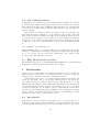
5.5
Position of the Selection Locus
Selected Locus
-0.5
Neutral Locus
0
1
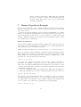
Figure 1: Figure of the locus model. The neutral loci can be anywhere on the
line, and there can be more than one. However by default, the neutral locus is
0 to 1 and the selected locus is at 0. The recombination rate is per unit of the
“locus line”. In this figure, the selected locus is at −0.5. The recombination
probability between 0 and 1 is twice the recombination probability between −0.5
and 0. Note that you can set the selected locus to be in the Neutral locus.
The position of the selected locus relative to the neutral loci is controlled
with the -Sp switch. The number is the position on the sequence line, while
the default neutral locus starts at zero and extends to 1. The default position
is zero. Figure 1 shows the relationship between the position and the default
neutral loci. We can adjust the recombination between the neutral locus and
selected locus by positioning the selected locus further away from the neutral
locus. Using this, we can position the neutral loci relative to the selected locus
to get the desired within locus recombination, and between locus recombination,
respectively. We can also position the selected locus inside the neutral locus if
we desire. By default the state of the selected locus is not part of the observable
mutations. However the -Smark switch will then include the selected locus in
the output mutations.
5.6
Deme and Time Dependent Selection
We include selection in the same way as with a single deme. However, we can
control selection strength in each subpopulation separately. This is interesting
when considering deme specific selection effects such as local adaptation. The
switch is -Sc and has the following syntax:
-Sc time deme SAA SaA Saa
Time is pastward and specifies the time that this switch takes effect. The effect
extends pastward indefinitely. If we use a time other than zero (sampling time),
the -SF option must also have the same time and there must be no changes to any
parameters pastward from that point. The deme is the deme label and SAA SaA
Saa are the selection strengths for the allele in homozygote and heterozygote
configurations. We must still specify the -SI or -SF switches to turn selection
on.
11
5.6.1
Example
We use the same parameters as the previous example. Only, we assume that the
allele is weak and purely recessive in the second deme (no selection on heterozygotes), while it is strong and almost completely dominant in the first deme has
almost equal selection strength for both the homozygotes and heterozygotes.
The command line is as follows:
>msms -N 10000 -ms 10 100 -t 5 -I 2 6 4 1 -n 2 .5 -m 1 2 2
-SAA 1000 -SaA 900 -Sc 0 2 500 0 0 -SF 0
We set the selection strength to 1000 and 900 for homozygotes and heterozygotes
respectively globally. We then change the selection parameters for deme 2 with
the -Sc switch to 500 and 0 respectively and condition on fixation at sampling
time.
6
Summary of options
Print out options documentation. This is often more up
to date than this document. If you are unsure of a option,
this provides invaluable “live” documentation.
-ms nsamples nrep The total number of samples and number of replicates. The
-ms can be omitted if these are the first two arguments.
-N Ne
Set Ne , note that event times are in discrete generation
times in units of 4Ne . Not required if there is no selection.
-t θ
Set the value of θ = 4Ne µ
-s s
Condition on the number of segregating sites. Just a little
slower than using -t and uses more memory.
-T
Output gene trees.
-L
Output tree length statistics.
-r ρ [nsites]
Set recombination rate ρ = 4Ne r where r is the recombination rate between the ends of a unit length sequence.
If nsites are omitted then an infinite sites recombination
model is used.
-G α
Set growth parameter of all populations to α.
-I npop n1 n2 . . . [4Ne m] Set up a structured population model. The sample
configuration must add up to the same total number of
samples as specified by -ms.
-n i x
Set the size of subpopulation i to xNe .
-g i αi
Set the growth rate of subpopulation i to αi .
-m i j Mij
Set the (i, j) element of the migration matrix to Mij .
-ma M11 . . .
Set the entire migration matrix.
-eM t x
Set all elements of the migration matrix at time t to x/(npop−
1)
-es t i p
Split subpopulation i into subpopulation i and npop+1
pastward. Each lineage currently in subpopulation i is retained with probability p, otherwise it is moved to the new
-help
12
population. The migration rates to the new subpopulation
are zero and its population size is set to Ne .
-ej t i j
Join subpopulation i to subpopulation j. All migration
matrix entries with subpopulation i are set to zero. The
population size of i is also set to zero. With selection this
population is ignored pastward from this time.
WARNING: This switch behaves differently from ms in the
strict definition. We consider that most people expect that
-ej is modeling a split in forward time and hence the deme
i is turned off pastward.
-e[X] t . . .
Set some parameter pastward from time t. Here [X] can
be any of G g n m ma and the meaning is defined as for the
normal command, for example -en t i x sets the population
size of deme i to xNe pastward from time t.
′
′
-l n a1 a1 . . . an an Set the neutral loci starting and stopping positions for n
′
loci. Note that must be ai < ai+1 for all i and that there
must be 2n values. All parameters assume a sequence
length of 1. This other parameter needs to be scaled accordingly.
-SAA αAA
Set the selection strength of the homozygote in units of
2Ne s.
-SAa αAa
Set the selection strength of the heterozygote in units of
2Ne s.
′
-Smu 4Ne µ
Set the forward mutation rate for the selected allele. That
is the mutation from the wild type a to derived type A.
′
-Snu 4Ne ν
Set the backward mutation rate for the selected allele. That
is the mutation from the selected type A to the wild type
a.
-Sp x
Set the position x in the sequence of the selected allele.
-Sc t i αAA αAa αaa Set the selection strength in deme i to the specified values
pastward from time t.α is in units of 2Ne s
-SF t
-SF t f
-SF t i f
Set the selection simulation stopping condition to fixation
at time t pastward from sampling time. t is time into the
past, i is the deme and f is the frequency. The first case
assumes fixation across all populations, the second case assumes frequency is across all populations. Selection is not
used forward in time from this point. It is up to the user
to ensure that the parameters permit the model to always
go to fixation, otherwise it will keep simulating till it runs
out of memory.
Note the demographic model must be time invariant for
this option to work properly.
-SI t npop x1 x2 . . . Set the start of selection to time t forward in time from
this point. The initial frequencies of the beneficial allele
13
are x1 , x2 , . . .. Note that this option is not compatible with
-SF.
-Smark
Include the selected locus in the mutation output.
-oTPi w s [onlySummary] Output windowed θ estimates (both Wattersons and
π based estimators) and Tajima’s D with window size w and
step size s. If onlySummary, then only the averages of all
replicates are output. The output format is a table formatted as follows: The first column is the bin position. The
second column is the Watterson’s θ estimator. The third
column is the π 5 estimator and the last column is Tajima’s
D. The summary also contains the standard deviations for
the previous data column. Thus, column 3 is the standard
deviation of the Wattersons θ estimators.
-oOC
Output the number of origins of the beneficial allele in the
sample. A count of 0 or 1 means a hard sweep if conditioned
on fixation.
-tt -oAFS [jAFS] [onlySummary] Output allele frequency spectra. If the jAFS
option is specified, all pairwise deme joint frequency spectra
are output.
-oTrace
Print the frequency trajectory of the forward simulations.
The first column is the time in 4Ne generations pastward
from present. Then each column is the relative frequency
of the beneficial allele in each deme. This format is the
same as required when specifying a trajectory.
-Strace f ilename Rather than simulate the forward trajectory, specify the
trajectory in a text file. The format of the -oTrace option
is valid for input. Note that you must include “unused”
demes produced with -ej or -es options even if the frequency is zero. Also it is not required to specify every
generation. Just a time and frequencies in a decreasing
order. msms will use linear interpolation for generations
between specified time points.
-threads n
Specify the number of threads to use. This permit very
easy use of multicore machines. The number of threads
should be only as much as you have cores available. This
will increase memory by the same factor as threads, so 2
threads will use twice as much memory as one. Also this
is not effective if each simulation is very fast, as the cores
spend most of their time waiting to output data.
-seed v
Set the seed. The seed is very different from ms since msms
uses quite a different random number generator. This is a
64 bit number that can be specified either in hex with a
0x prefix or normal decimal. msms goes to some effort to
randomize the seed value so you you don’t need to set seed
5 average
pairwise difference
14
values on cluster environment. When using the -threads
the seed for “iteration n” will be the same and hence give
the same result. However the order of reported results will
generally be different.
7
Human Population Example
We now give an example of how to build arbitrary models from the ground up.
We first consider the case with no selection, and then add selection as the last
part of the exercise.
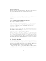
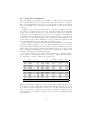
The model is shown in Figure 2 and comes from (Gutenkunst et al., 2009).
There are 4 populations with admixture, exponential population growth, a bottleneck and migration. We will not concern ourselves too much with specific
values for different parameters, but rather keep them as simple values to make
the example easier to understand.
Events at Time Zero
We start with 4 sampled populations with a sample size of 20 from each population and some reasonable initial Ne . In this case, we consider high mutation
rates with moderate recombination. We have:
>msms -N 10000 -ms 80 1000 -I 4 20 20 20 20 0 -t 100 -r 100 1000
But now, we must consider admixture. The CEU population is mixed with the
MXL population. If we use the -es split switch, it creates a new deme 5 rather
than joining some of the samples from deme 3 (CEU) to 4 (MXL). But, we can
join deme 4 to the new deme at the same time.
-es 0 3 .5 -ej 0 4 5
So at time zero, samples from deme 3 stay in deme 3 with probability 0.5.
Otherwise, the samples or lineages are moved to the newly created deme 5.
Since deme 5 is really the MXL that we have sampled, we join deme 4 to deme
5 as well. Note that deme 5 will have no migration parameters and currently,
nothing has any migration set.
Next, we consider growth and population sizes. CHB, CEU and MXL are
growing exponentially. We set them to 10, 100 and 200 respectively as follows
-g 2 10 -g 3 100 -g 5 200
Note that we don’t set the 4th deme since we joined it to deme 5. Now we set
the initial population sizes relative to Ne . Since YRI is the largest population,
we assume that’s our nominal Ne value. Again we assume the population sizes
are .9, 2, and 11. Note that these populations are growing rapidly.
-n 2 .0 -n 3 2 -n 5 11
15
A
B
ma
mb
mc
YRI
CHB
CEU
MXL
Figure 2: A model of human demographics.
Finally, we need to set the migration rates mc and mb. We set these to 5
and 2 respectively with the following.
-m 1 3 5 -m 3 1 5 -m 1 2 2 -m 2 1 2
Note we assume symmetric migration rates, so we need to use two -m stitches
per deme pair.
First Event Pastward.
The first pastward event is the MXL population joining the CEU population.
We assume that this happens 1600 generations into the past. The t1 time
is therefore 1600/(4Ne ) = 1600/40000 = 0.04. This is a deme joining event
pastward, so we add the following to our command line.
-ej 0.04 5 3
Nothing else changes so that’s all that’s required.
Second Event Pastward
The second event is the joining of the CHB deme with the CEU demes. We
set this to be 2000 generations into the past so t2 = 0.05. However, this time
migration changes as does population size. We also note that there is no longer
any exponential growth. We set the B population to have the size of YRI, and
the migration rate ma is 12. Thus, we add
-ej 0.05 3 2 -en 0.05 2 .5 -em 0.05 1 2 12 -em 0.05 2 1 12
The -en switch sets the growth rate to zero, so we do not need to use any -eg
switch.
16
Third Event Pastward.
We have come to the last population merger. This happens 6000 generations
into the past. There is nothing else to set in this case, so we have.
-ej 0.15 2 1
Last Event
Finally, we have a bottleneck 8000 generations ago where the population was
reduced to half its nominal value. The last option to add is.
-en 0.2 .5
7.1
Complete Command Line & Selection
The complete command line is therefore
>msms -N 10000 -ms 80 1000 -I 4 20 20
-es 0 3 .5 -ej 0 4 5 -g 2 10 -g 3 100
-n 5 11 -m 1 3 5 -m 3 1 5 -m 1 2 2 -m
-ej 0.05 3 2 -en 0.05 2 .5 -em 0.05 1
-ej 0.15 2 1 -en 0.2 .5
20 20 0 -t 100 -r 100 1000
-g 5 200 -n 2 .0 -n 3 2
2 1 2 -ej 0.04 5 3
2 12 -em 0.05 2 1 12
We claim there is selection in the CEU deme only and that standing variation
was initially zero with a medium forward mutation rate at the beneficial locus.
We only have to add the following.
-SI 0.05 5 0 0 0 0 0 -Sc 0 3 100 50 0 -Smu 0.1
First, the -SI option took the number of demes to be 5 despite the fact that
we “joined” one. This is because it still exists and we could set its population
size to a nonzero value. It is also important to note that the -SI option is the
only option to work in forward time. That is, selection starts at time 0.05 till
the present. While the -Sc option works pastward, in this case from sampling
time. Finally, we set the mutation rate to 0.1.
8
Trouble shooting
Unfortunately things go wrong. Many of the times its is simply something wrong
with the command line options. Occasionally its a bug. Either way msms tries
as hard as it can to tell you what is wrong. However this is harder than it looks
and often the error message can be cryptic or even misleading. This is a area
that is constantly improving so ensure you have the latest release.
Often msms puts out a lot of error messages. This is to make it easier for
us to pinpoint bugs when people give bug reports. Generally however you only
need to pay attention to the first few lines or so and can safely ignore the rest.
17
8.1
has an incorrect number of arguments.
This error comes up frequently. It has a number of causes and not all of them
are in fact the wrong number of arguments. Currently you should check if you
do in fact have the correct number of arguments and that all switch’s are typed
correctly. Note that all switch’s are case sensitive.
The reason this error comes up even if you do have the correct number of
arguments is that the next switch is typed wrong. The parsing code then thinks
this switch it does not know about belongs to the previous switch. The following
is a example.
msms 20 1000 -tt 5
msms does not identify the -tt and the error message is:
has an incorrect number of arguments.
options you tried was:
20 1000 -tt 5
Option help:
-ms nsam replicates
Alias:
Required
Sets sample size and replicates.
You can see that under you tried was is the -tt. This tells you that the switch
is unrecognized. We are currently working on improving the parsing code to deal
with this situation better. So at least it gives a good error messages.
8.2
Cannot condition on fixation times ...
You have used the -SF switch with a model that changes over time. This does
not work as msms use a forward simulation for the allele frequencies not a
pastward process like the coalescent. There is no known pastward process for
selection trajectories for the general case. The only option is to use the -SI
option instead.
8.3
Model does not permit full coalescent of linages.
This is most frequently caused by having demes with samples without migration
between them. Since the lineages cannot migrate into the same deme, they
cannot coalesce and the simulation would run forever. In this case msms has
detected this situation and has thrown an error.
Generally any situation where lineages cannot coalesce should give this error.
However it is often hard to detect and may just run at 100% CPU, never running
out of memory or finishing.
18
8.4
Out of Memory Errors
Sometimes an out of memory errors is a indication that something else is wrong.
A common cause is when conditioning on fixation in a case where the beneficial
allele will never fix. The forward simulation will just run forever, or until it runs
out of memory. It is important to eliminate this case first before increasing the
memory available.
However there are situations where one really does run out of memory and
increasing the memory available to msms will solve the problem. The first
thing to know is that by default msms will not try and just use all the memory
of your system but will give a out of memory error if it needs more than 256
megabytes of ram. Most modern systems have much more than this. It is easy
to tell msms to use more, but this must be done by directly invoking java like
so.
java -Xmx500M -jar lib/msms.jar
This is assuming that you are in the msms directory. This increases the ram
available to 500 megabytes. Generally setting this as high as all your ram my
not be a good idea. As once msms uses all that ram, your computer could
become so slow that appears to be frozen.
8.5
Help My Problem is not here
Please submit a bug report to the mailing lists [email protected].
Remember to include the full command line you are using.
9
Performance
In this section, we demonstrate the current performance of the code with and
without selection and relative to ms. This should give some idea of what parameters tend to dominate performance when using selection.
Unfortunately, there are a lot of parameters that can affect performance and
details are important. We do not present a full study here, but merely use
some simple examples to illustrate general trends. We should also note that
different hardware will also perform differently, and different environments such
as operating systems can have an effect. Importantly, the version of java used
can have a big impact on performance of msms. Generally, the latest version
should be used as it includes the latest optimizations. For example Java 1.6.0u12
was about 10% to 20% faster than Java 1.6.0. Also, if one is running on a 64bit
machine, the 64bit version of java should be used.
9.1
Introduction
Performance of msms is considered important, but not at the expense of correctness. Because this is a selection simulator, the methods that work best for
reasonable parameter ranges under selection can be less optimal for other cases.
19
If such trade-offs occur, we have tried to optimize the code to improve run times
for parameter ranges where simulations are generally slow (in particular, large
recombination rates), even if this comes at the expense of somewhat longer run
times for parameter sets where simulations are very fast anyway. Hence, in some
cases ms will be faster than msms for neutral models, in particular with low
recombination.
All times were collected on an AMD64 X2 Dual Core Processor 6000+, using
Sun Java 1.6u18 64bit and gcc 4.2.3 ruining Linux. ms was compiled with a
-O3 compiler option.
9.2
Neutral models
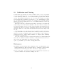
Lets first consider neutral models and compare with ms. The results for representative parameter sets are shown in table 1. We note that while msms is
slower than ms in some cases, this only occurs in parameter regions where both
programs are fast (10000 replicates under 1 minute). In these cases programs
that print out a lot of data to the screen, such as ms and msms are generally IO
limited (first 4 rows). However once we increase tree depth, recombination or
both, msms is faster than ms, almost 6 times faster for one example. For long
sequence lengths and for migration histories that result in deep trees, msms is
a good choice even with neutral models.
These results also show which factors influence run times most strongly. Its
clear from table 1 that recombination has by far the biggest influence. This
is even more true when selection is also considered. Migration also has some
influence on performance. However, the primary reason is that the deeper tree
results in more recombination events.
n
100
100
100
100
100
10
10
10
reps
10000
10000
10000
10000
1000
1000
1000
1000
migration
1
1
1
-
ρ
10
10
100
100
500
500
500
1000
ms time
14.6
33.9
92.1
424.4
222.5
95.0
742.1
495.0
msms
19.9
46.1
139.4
422.7
167.9
28.2
125.9
94.0
ratio
0.73
0.74
0.66
1.0
1.325
3.33
5.9
5.27
Table 1: Performance of ms compared to msms for different parameters. The
number of recombination sites was 10000 and θ = 10. Cases with migration
have 2 demes with an equal number of samples from each. Times were collected
on an AMD64 X2 Dual Core Processor 6000+, using Sun Java 1.6u18 64bit and
gcc 4.2.3. ms was compiled with a -O3 compiler option. Times are in seconds.
We note that msms does very well with deeper trees and high recombination.
However ms is still faster for low recombination rates.
20
9.3
Selection Performance
Selection influences performance in a number of different ways. Principally,
the forward simulation step needs both CPU time and memory to construct.
The coalescent simulation is also slower because it must condition on frequency
trajectory. Finally, selection can have a large influence on the expected depth
of the tree.
Results for selection are shown in table 2. For these comparisons, we use
the same set of parameters as for table 1. The first result is that with high
selection the run times can in fact be less than in the neutral case. This can
be understood by realizing that a large part of performance is dominated by
recombination and that high levels of selection result in short coalescent trees
at the selected locus. There are thus less recombination events. High selection
is also faster for the forward simulation as a sweep takes less generations and
the forward simulation can use less memory and CPU cycles.
Table 2 also shows that run times increase substantially if selection strength
is reduced. This is dramatic for α = 10, where simulations take over 6 times
longer than under neutrality However, migration does not influence the performance under selection more than under neutrality, and we note that, overall,
the performance is still similar to the neutral case. Generally, recombination is
again the dominant factor affecting run times.
From these results, we can conclude that it is reasonable to simply add selection to whatever demographic scenario one wishes to study. The performance
is comparable to neutral evolution for the most part.
n
100
100
100
100
100
10
10
10
10
10
10
reps
10000
10000
10000
10000
10000
1000
1000
1000
1000
1000
1000
m
1
1
1
-
ρ
10
10
10
100
100
500
500
500
500
500
500
α
100
1000
1000
1000
1000
1000
1000
1000
1000
100
10
Ne
10000
10000
105
10000
10000
10000
10000
105
105
105
105
neutral
19.9
19.9
19.9
139.4
422.7
28.2
28.2
28.2
125.9
125.9
28.2
selection
32.7
12.6
35.5
147.3
452.9
21.3
21.3
23.9
105.6
190.7
194.1
ratio
0.62
1.58
0.56
0.94
0.93
1.32
1.32
1.18
1.19
0.66
0.15
Table 2: Performance with selection. We use the same parameters as for table
1. In all cases, we are conditioning on fixation at sampling time (-SF 0), and do
not consider recurrent mutation at the selected locus. Note that large selection
improves performance compared to the neutral case. This is because the tree is
shorter and fewer recombination events occur. Note that recombination is still
the dominant.
21
10
Validation and Testing
A small testing program is also included. This is used to test for regressions
and bug discovery. Currently, we compare the mean and standard deviation
of some summary statistics to other well-established programs with different
options. The summary statistics we use are average tree length, tree height,
and segregating sites and singletons. These are good at discriminating errors in
the code while being quick to calculate. For example if the tree height statistic
matches, but the segregating sites do not, we can assume that there is some bug
in the mutation code.
The tests are not rigorous statistically speaking. Currently, more statistically
sound testing is done with R and is difficult to automate. However, despite the
fact that these simple tests are not rigorous and perhaps some statistics appear
redundant, they have been shown to discriminate whenever more thorough tests
have failed. That is for cases where full statistical tests fail, these simple tests
also fail.
It is important to note that the tests are probabilistic in nature. Therefore,
we expect test failures by random chance alone. This becomes more pronounced
with more tests due to multiple testing. Several executions of the testing program should however result in different failures or complete passes, assuming
no bugs have been introduced.
In order to run the tests, there is a script in the bin directory called simpleTest
that works on both Mac and Linux. Otherwise on all platforms, inside the msms
directory the following will also invoke the test program:
>java -cp lib/msms.jar at.mabs.testing.BasicTests
References
Gutenkunst, R. N., Hernandez, R. D., Williamson, S. H., and Bustamante, C. D.
(2009). Inferring the joint demographic history of multiple populations from
multidimensional SNP frequency data. PLoS Genet, 5(10), e1000695.
Hudson, R. R. (2002). Generating samples under a Wright-Fisher neutral model
of genetic variation. Bioinformatics, 18(2), 337–338.
22