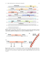
1
Modelling of GPCRs
www.allitebooks.com
Andrea Strasser • Hans-Joachim Wittmann
Modelling of GPCRs
A Practical Handbook
2123
www.allitebooks.com
Andrea Strasser
University of Regensburg
Institute of Pharmacy
Dept. of Pharm./Med. Chemistry
Regensburg
Germany
Hans-Joachim Wittmann
University of Regensburg
Faculty of Chemistry and Pharmacy
Regensburg
Germany
ISBN 978-94-007-4595-7
ISBN 978-94-007-4596-4 (eBook)
DOI 10.1007/978-94-007-4596-4
Springer Dordrecht Heidelberg London New York
Library of Congress Control Number: 2012938366
© Springer Science+Business Media Dordrecht 2013
No part of this work may be reproduced, stored in a retrieval system, or transmitted in any form or by
any means, electronic, mechanical, photocopying, microfilming, recording or otherwise, without written
permission from the Publisher, with the exception of any material supplied specifically for the purpose of
being entered and executed on a computer system, for exclusive use by the purchaser of the work.
Printed on acid-free paper
Springer is part of Springer Science+Business Media (www.springer.com)
www.allitebooks.com
Preface
Biological cells function as elementary building blocks for living individuals. All
compounds, essential for establishing and maintaining life processes are to be produced inside the cells. This makes it necessary for molecules and ions to pass the cell
membrane in order to take part or to support the appropriate biochemical reactions.
Furthermore, a lot of regulatory processes control the complicated sequences of the
molecular reaction cycles and signal cascades and may be influenced by information
in form of physical effects or chemical compounds coming from the environment
of the individuals. So, all what we call life is subject to biochemical processes and
may be described by thermodynamic and kinetic concepts. Energetic and entropic
aspects were therefore used in a larger extent to explore the behaviour of chemical
compounds addressing G protein-coupled receptors residing in the cell membrane. In
this context, drug design in the past was done by chemical synthesis and pharmacological testing afterwards, hoping to obtain a powerful new active compound. But in
order to have specific drugs, exhibiting a minimum of side effects and to reduce costs
and time of research and production, a deeper insight onto processes linked with the
interaction of ligands and receptors on molecular level is necessary. So, nowadays a
scientist working on the field of drug design has to use the physicochemical concepts
to successfully predict the properties of compounds. But an increasing knowledge of
the processes determining the behaviour of the interaction between ligands and receptors reveal a great complexity of this research field. Computational methods have
to be used in order to describe quantitatively the processes setting up the network of
ligand-receptor-interaction and the related signal cascades. Working on the field of
GPCRs, theoretical concepts have to be developed and a large number of related programs have to be designed and it turns out that the operation system UNIX/LINUX
is the best solution to do all this work in a highly efficient manner. Thus, we got the
idea to present not only a review of methods and results concerning the modelling of
GPCRs, but to establish a practical guide for researchers interested in this field. Realizing the great importance of the work in computing, we included a chapter designed
as an overview of the most important UNIX/LINUX commands and present a lot of
solutions concerning computational problems. We hope, researchers will comprehend the benefit of the operating system. All commands and scripts presented in this
book were developed very carefully. Nevertheless we do not give any warranty for
correctness.
v
www.allitebooks.com
Contents
1
Introduction . . . . . . . . . . . . . . . . . . . . . . . . . . . . . . . . . . . . . . . . . . . . . . . . . . .
1
2
G Protein Coupled Receptors . . . . . . . . . . . . . . . . . . . . . . . . . . . . . . . . . . . .
2.1 Structure of GPCRs . . . . . . . . . . . . . . . . . . . . . . . . . . . . . . . . . . . . . . . . .
2.2 Different GPCR Families . . . . . . . . . . . . . . . . . . . . . . . . . . . . . . . . . . . .
2.3 Activation of GPCRs and Their Interaction with G Proteins . . . . . . . .
2.4 Important Internet Sources with Regard to GPCRs . . . . . . . . . . . . . . .
5
5
5
7
10
3
Sequence Alignment and Homology Modelling . . . . . . . . . . . . . . . . . . . .
3.1 Selection of a Template . . . . . . . . . . . . . . . . . . . . . . . . . . . . . . . . . . . . . .
3.2 Crystal Structures of GPCRs . . . . . . . . . . . . . . . . . . . . . . . . . . . . . . . . .
3.3 Amino Acid Sequences and Sequence Alignment . . . . . . . . . . . . . . . .
3.3.1 Amino Acid Sequences – Where to Get From? . . . . . . . . . . . .
3.3.2 Ballesteros Nomenclature . . . . . . . . . . . . . . . . . . . . . . . . . . . . .
3.3.3 Amino Acid Sequences – Templates . . . . . . . . . . . . . . . . . . . . .
3.3.4 Sequence Alignment . . . . . . . . . . . . . . . . . . . . . . . . . . . . . . . . . .
3.4 Homology Modelling . . . . . . . . . . . . . . . . . . . . . . . . . . . . . . . . . . . . . . .
3.4.1 Modelling of the Transmembrane Domains . . . . . . . . . . . . . . .
3.4.2 Modelling of Loops . . . . . . . . . . . . . . . . . . . . . . . . . . . . . . . . . .
3.4.3 Modelling of Internal Water . . . . . . . . . . . . . . . . . . . . . . . . . . . .
3.4.4 Modelling of the C-Terminal Part of the Gα Subunit or the
Whole Gα Subunit . . . . . . . . . . . . . . . . . . . . . . . . . . . . . . . . . . .
3.4.5 Refinement of the Receptor Model . . . . . . . . . . . . . . . . . . . . . .
13
13
14
18
18
20
20
22
23
23
23
25
4
Construction of Ligands . . . . . . . . . . . . . . . . . . . . . . . . . . . . . . . . . . . . . . . .
29
5
Lipids . . . . . . . . . . . . . . . . . . . . . . . . . . . . . . . . . . . . . . . . . . . . . . . . . . . . . . . .
5.1 Structure of Lipids . . . . . . . . . . . . . . . . . . . . . . . . . . . . . . . . . . . . . . . . . .
5.2 Structure of the Phospholipid Bilayer . . . . . . . . . . . . . . . . . . . . . . . . . .
5.3 Lipid Bilayer Models Used in Molecular Modelling . . . . . . . . . . . . . .
5.4 Internet Sources for Lipid Bilayer Models . . . . . . . . . . . . . . . . . . . . . .
5.5 Embedding a GPCR into a Lipid Bilayer . . . . . . . . . . . . . . . . . . . . . . .
37
37
39
40
40
42
25
26
vii
www.allitebooks.com
viii
6
7
Contents
Minimization and Molecular Dynamics . . . . . . . . . . . . . . . . . . . . . . . . . . .
6.1 Generating a Complete Model of the Interesting GPCR . . . . . . . . . .
6.2 Embedding the GPCR in a Lipid Bilayer . . . . . . . . . . . . . . . . . . . . . .
6.3 Solvation of the Lipid-GPCR-Complex, Achiving
Electroneutrality of the Simulation Box and Minimization . . . . . . .
6.4 Molecular Dynamic Simulation of your System . . . . . . . . . . . . . . . .
59
60
60
Calculation of Gibbs Energy of Solvation . . . . . . . . . . . . . . . . . . . . . . . . .
7.1 Theory – Link Between Microscopic and Macroscopic World . . . .
7.1.1 Statistical Mechanical Basics . . . . . . . . . . . . . . . . . . . . . . . . .
7.1.2 From Potential Energy to the Chemical Potential . . . . . . . . .
7.1.3 The Concept of the Coupling Parameter Within MD
Simulations . . . . . . . . . . . . . . . . . . . . . . . . . . . . . . . . . . . . . . . .
7.2 Examples – Conceptual and Practical Considerations . . . . . . . . . . . .
7.2.1 Example 1: Ethanol in Water – Conceptual
Considerations . . . . . . . . . . . . . . . . . . . . . . . . . . . . . . . . . . . . .
7.2.2 Example 2: Ligand-Receptor-Complex and
Affinity – Conceptual Considerations . . . . . . . . . . . . . . . . . .
7.2.3 Example 1: Ethanol in Water – Practical Considerations . . .
7.2.4 Example 2: Gibbs Energy of Binding . . . . . . . . . . . . . . . . . .
75
75
75
77
60
62
79
80
80
83
85
99
8
Special Topics in GPCR Research . . . . . . . . . . . . . . . . . . . . . . . . . . . . . . . . 105
8.1 Interaction Between a GPCR and the Gα-subunit . . . . . . . . . . . . . . . 105
8.2 Process of Ligand Binding from the Extracellular Side
into the Binding Pocket of a GPCR . . . . . . . . . . . . . . . . . . . . . . . . . . 112
9
Force Fields . . . . . . . . . . . . . . . . . . . . . . . . . . . . . . . . . . . . . . . . . . . . . . . . . . .
9.1 The Force Field Energy . . . . . . . . . . . . . . . . . . . . . . . . . . . . . . . . . . . .
9.1.1 The Stretching Energy . . . . . . . . . . . . . . . . . . . . . . . . . . . . . . .
9.1.2 The Bending Energy . . . . . . . . . . . . . . . . . . . . . . . . . . . . . . . .
9.1.3 The Torsional Energy . . . . . . . . . . . . . . . . . . . . . . . . . . . . . . . .
9.1.4 The van der Waals Energy . . . . . . . . . . . . . . . . . . . . . . . . . . . .
9.1.5 The Electrostatic Energy . . . . . . . . . . . . . . . . . . . . . . . . . . . . .
9.2 The All-atom-concept and Site-concept . . . . . . . . . . . . . . . . . . . . . . .
9.3 The Force Field Parameters . . . . . . . . . . . . . . . . . . . . . . . . . . . . . . . . .
121
121
121
122
123
124
124
124
125
10 Thermodynamics of Ligand-Receptor Interaction . . . . . . . . . . . . . . . . . .
10.1 Motivation . . . . . . . . . . . . . . . . . . . . . . . . . . . . . . . . . . . . . . . . . . . . . . .
10.2 Ligand-Receptor Model . . . . . . . . . . . . . . . . . . . . . . . . . . . . . . . . . . . .
10.3 Thermodynamic Basics . . . . . . . . . . . . . . . . . . . . . . . . . . . . . . . . . . . .
10.4 Evaluating Ho and So . . . . . . . . . . . . . . . . . . . . . . . . . . . . . . . . . . .
10.5 Special Topics . . . . . . . . . . . . . . . . . . . . . . . . . . . . . . . . . . . . . . . . . . . .
131
131
131
132
136
138
www.allitebooks.com
Contents
ix
11 Important UNIX/LINUX Commands . . . . . . . . . . . . . . . . . . . . . . . . . . . . .
11.1 Some Basic Aspects of the Operating System UNIX/LINUX . . . . .
11.2 The Use of Shell Operators and Meta-Characters in Tcsh
Environments . . . . . . . . . . . . . . . . . . . . . . . . . . . . . . . . . . . . . . . . . . . . .
11.3 Shell Substitutions . . . . . . . . . . . . . . . . . . . . . . . . . . . . . . . . . . . . . . . .
11.3.1 File Name Substitution . . . . . . . . . . . . . . . . . . . . . . . . . . . . .
11.3.2 Variable Substitution . . . . . . . . . . . . . . . . . . . . . . . . . . . . . . .
11.3.3 Command Substitution . . . . . . . . . . . . . . . . . . . . . . . . . . . . .
11.3.4 Protection Mechanism for Meta-Characters
of the TC-Shell . . . . . . . . . . . . . . . . . . . . . . . . . . . . . . . . . . . .
11.4 Discussion of Selected LINUX Commands . . . . . . . . . . . . . . . . . . . .
11.5 Loops Statements of the Tcsh Shell . . . . . . . . . . . . . . . . . . . . . . . . . .
11.6 Working with Shell Scripts . . . . . . . . . . . . . . . . . . . . . . . . . . . . . . . . . .
11.7 A More Extensive Example . . . . . . . . . . . . . . . . . . . . . . . . . . . . . . . . .
139
139
139
140
141
141
143
143
144
152
153
155
Appendix . . . . . . . . . . . . . . . . . . . . . . . . . . . . . . . . . . . . . . . . . . . . . . . . . . . . . . . . . 161
References . . . . . . . . . . . . . . . . . . . . . . . . . . . . . . . . . . . . . . . . . . . . . . . . . . . . . . . . 209
Index . . . . . . . . . . . . . . . . . . . . . . . . . . . . . . . . . . . . . . . . . . . . . . . . . . . . . . . . . . . . 217
www.allitebooks.com
Chapter 1
Introduction
The knowledge about conformation of proteins and distinct interactions between
a ligand and it’s target protein is necessary to explain pharmacological data on a
molecular level. Additionally, based on this knowledge, it may be possible to develop new, potent drugs more efficiently. But how get these insights on a molecular
level? Several experimental techniques, like mutagenesis studies combined with
pharmacological investigations may give hints about amino acids, being important
for stability of a protein or being important for the interaction between ligand and
protein. But these studies exhibit no information about energetics and hydrogenbond-networking for example. Other techniques, like determination of structures
of proteins or protein-ligand-complexes by NMR or crystallography are very useful to obtain information about secondary, tertiary or quartary structures of proteins
(http://www.pdb.org). However, these experiments are time-expensive and cannot be
performed for each system of interest like on an assembly line. Additionally it has to
be taken into account, that crystal structures represent a solid phase, but proteins are
in general in solution and exhibit a kind of dynamical behaviour. This is taken into
account by molecular dynamic simulations of a protein in its natural surrounding.
Additionally, with several distinct molecular modelling techniques, ligand-receptor
interactions for example, can be simulated in a reasonable time and insights onto
interactions on molecular level can be obtained. Furthermore, some techniques, like
3D-QSAR (Brown et al. 2006; Dudek AZ et al. 2006; Gedeck et al. 2008; Scior T
et al. 2009) allows predicting affinities also in context with GPCRs (Strasser et al.
2010a; Silva et al. 2011). However, molecular modelling results should be, when
ever possible, compared with experimental data in order to judge predictive quality.
To combine the experimental results with computational methods in order to understand and moreover to predict the behaviour of systems involving chemical reactions,
it is necessary to establish a link between macroscopic quantities, like equilibrium
and rate constants, thermodynamic quantities like H o and S o , which are available
from experimental methods (Leavitt S et al. 2001; Wittmann et al. 2009; Torres et al.
2010) and microscopic properties, like energy levels, which result from the interactions of the nuclei and electrons comprising the distinct particles of the system of
interest. This task is not a simple one especially when certain properties for example of a ligand interacting with the receptor are to be depicted as thermodynamical
A. Strasser, H.-J. Wittmann, Modelling of GPCRs,
DOI 10.1007/978-94-007-4596-4_1, © Springer Science+Business Media Dordrecht 2013
www.allitebooks.com
1
2
1 Introduction
quantities. So, there were a lot of efforts in the past to classify ligands as agonists or
antagonists with the help of H o and S o . One attempt to distinguish between the
two groups of ligands is based on the term enthalpy or entropy driven association process. Enthalpy driven means H o < 0 and S o < 0, entropy driven is indicated by
H o > 0 and S o > 0, whereas H o < 0 and S o > 0 is called enthalpy-entropy
driven (Weiland et al. 1979; Wittmann et al. 2009). But by investigating the extensive
data material no definite discrimination between agonists and antagonists is possible
on this basis. The crucial point results from the fact that H o and S o determine
the affinity of a ligand investigated in a binding assay. But if we talk about agonists
or antagonists, we put our focus on the efficacy, which will be determined from corresponding assays. To combine binding properties like H o or S o with quantities,
describing the efficacy will not lead to satisfactory results. Thus, is there a chance at
all to predict the binding behaviour of a ligand on the base of the thermodynamical
concept, discussed in Chap. 10? As a first step, we have to establish a binding model
based on our knowledge or intuition of the interaction between the ligand and the
receptor. X-ray based structures are the best choice up to now to get structures of the
interesting biochemical system, which would then be utilized to calculate H o and
S o or rate constants for comparison with the experimentally determined values and
to validate a particular model. Making use of statistical mechanical concepts (see
Chap. 7.1), the central quantity is the potential energy of the system from which we
are able to calculate the phase integral and thereafter the chemical potential, which
governs the chemical behaviour of an arbitrary species. These concepts are adopted
in the framework of the quantum mechanical concept by calculating the so-called
partition sum (see Chap. 7.1). Here, we also have to define the potential energy
of the system of interest and then we have to solve the corresponding Schrödinger
equation to get the allowed energy levels. But up to now, it is impossible for such
large systems, comprised of ligand, receptor, membrane, water and ions to do such
ab initio calculations in an acceptable time. To simplify the calculation procedure, a
stable state is defined as a energy minimum of the so-called potential energy surface,
represented by the potential energy as a function of all coordinates of the particles
present in the system. Starting from a first guess of a structure, minimizing the potential energy with respect to the coordinates, will lead to a final structure from which
we are able to derive a set of properties. Even this modified procedure leads to a very
time consuming calculation. Thus, ab initio methods are not suitable to handle biochemical systems. However, sometimes, this method is used in context with GPCR
research (Carloni et al. 2002; Mehler et al. 2006; Jongejan et al. 2008). The so-called
semiempirical methods use potential functions based on some experimental insight
to find local minima across the potential energy surface (Stewart 1989; Stewart 2004;
Lipkowitz et al. 2007). This concept reduces the computational time but introduces
a new problem based on the choice of the semiempirical method, which seriously
influences the computed results. In order to get a very simple functional form of
the potential energy resulting in small computational times, molecular dynamics
(molecular mechanics) makes use of so-called force fields (see Chap. 9), which entirely depend on empirical quantities, so the quality of the results strongly depends
on the experimental parameters used to define the particular force field. To combine
www.allitebooks.com
Introduction
3
the well founded theoretical concept of quantum mechanics with the advantage of
a short computational time, hybrid methods, such as quantum mechanics/molecular
mechanics (QM/MM) concept are introduced (Monard et al. 1999). The interesting
part of the system is calculated using the principles of quantum mechanics, whereas
the remainder of the system is treated by the methods of molecular mechanics. To take
advantage of this method we have first to define the boundary between the “quantum
mechanical region” and “classical region” and secondly, we have to establish a connection between the two regions, which is done by introducing so-called link atoms.
A further improvement of the hybrid methods is developed in the framework of the
moving domain quantum mechanics/molecular mechanics (MoD-QMMM). To gain
deeper insight into the basics of the hybrid methods, the reader is referred to the literature (Gascon et al. 2006; Menikarachchi et al. 2008). Searching the potential energy
surface for minima, any of the mentioned methods will find only local minima. To
identify the most stable configuration of the system of interest, the global minimum
of the potential energy surface should be detected, but up to now, no reliable algorithm, solving this problem is available. Thus, to get enough information about the
system of interest, multiple scans have to be done from distinct starting structures.
But in this context, the question arises, whether these different configurations have
to be linked by equilibrium processes or not. Doing so, we will get a very large set of
structures from which we have to explain the interaction between the ligand and the
receptor. A further crucial problem appears, when the entropic contributions are to be
evaluated. Molecular mechanics methods totally lack the calculation of such terms,
whereas quantum mechanical based methods allow for estimating the entropy term
of a system in principle, which is given mainly by the vibration modes. So, if we deal
with a system comprised of N sites we have to determine 3 · N − 6 vibration modes,
i.e. for N = 10,000 there are nearly 30,000 vibrational terms to be computed. Further
on, there is another problem arising from the modes belonging to transition states.
Since we are interested in equilibrium states and get a lot of transition modes, we
have to change the geometry of our system in a way that only real vibrational modes
appear, which is a very tedious task. Many of the vibrational modes describe internal rotations around bonds, characterized by low frequencies and therefore make an
unacceptable large contribution to the overall vibration energy. An exact treatment
of this motion is not available up to now. The prediction of the entropy term S o
in this context is a very difficult matter and consequently the results are not reliable.
Because of this difficulties, in almost all studies, based on the mentioned methods,
also called single point calculations, only the potential energy terms or the allowed
energy levels of the system are used for a qualitative discussion of its behaviour.
To overcome the problems caused by single point calculations, molecular dynamic
studies (MD) on biological systems have to be carried out. These methods make use
of the equation of motion, introduced by Newton, to compute the time evolution
of a system. For calculating thermodynamical quantities, the reader is referred to
Chaps. 7 and 10. Up to now, processes with time constants in the range of some
μs are subject to MD simulations, so processes taking place with time constants in
the range of ms or larger, like diffusion processes in solutions, cannot be captured
by this method. Furthermore, force field methods are unable to handle processes
www.allitebooks.com
4
1 Introduction
accompanied by bond forming or bond breaking. Thus, the calculation of the Gibbs
energy, see Chap. 7, is limited to reactions leaving the molecule intact, e.g. solvation
processes. A completely different concept, known as “quantitative structure activity
relationship” does not deal with theoretically founded energy terms. Most often, the
“quantitative structure activity relationship” (QSAR) is used to predict for example
structures and association constants for biochemical systems (Strasser et al. 2010a;
Silva et al. 2011). Following this concept, a correlation is established between the
desired property of a system and leading variables for the training systems (Kubinyi
2011). Calculating the value of the leading variables for the system of interest provides the desired property with the help of the former correlation. However, it must
be emphasized that the better the system of interest corresponds to the data material
representing the training set the better the prediction of binding properties will be.
Chapter 2
G Protein Coupled Receptors
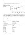
The G protein coupled receptors (GPCRs) represent one of the largest families of
proteins within the human genome and mediate several physiological and pathophysiological effects (Jacoby et al. 2006). GPCRs are of general interest with regard
to therapy of several diseases, since about 27 % of all drugs available on market are
addressing GPCRs (Fig. 2.1) (Wise et al. 2002; Overington et al. 2006).
Since a lot of literature is available with regard to GPCRs, only a short introduction
is given in this chapter.
2.1
Structure of GPCRs
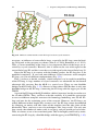
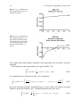
GPCRs are transmembrane receptors. Thus, they are located in the lipid bilayer. The
GPCRs consist of seven transmembrane α helixes, spanning through the membrane
from the extracellular to the intracellular part. The transmembrane domains are connected by intra- and extracellular loops. The N-terminus (amino terminus) is located
on the extracellular part, whereas the C-terminus (carboxy terminus) is located on
the intracellular part. Because of the structure, GPCRs are sometimes called “seven
transmembrane receptors” (“7 TM receptors”) (Fig. 2.2).
2.2
Different GPCR Families
GPCRs were divided into several families A–F (classes) and are described systematically (IUPHAR 2000; Fredriksson et al. 2003; Suwa et al. 2011, http://www.gpcr.
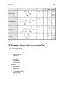
org). However, there are three main families A, B and C (Table 2.1). A more detailed
listing is given in the appendix GPCR Families (Source: http://www.gpcr.org/7tm).
Family A The family A GPCRs represents the largest GPCR family (IUPHAR 2000;
Ballesteros et al. 2001; Chalmers et al. 2002; Jacoby et al. 2006; Mustafi et al. 2009)
and is the one, which is mostly studied. The family A GPCRs, like biogenic amine receptors or (rhod)opsin (see appendix GPCR Families (Source: http://www.gpcr.org/
7tm)) are the most studied so far. A disulfide bridge between the E2-loop and the upper
part of TM III is typical for most of the family A GPCRs (Fig. 2.3). Additionally, most
A. Strasser, H.-J. Wittmann, Modelling of GPCRs,
DOI 10.1007/978-94-007-4596-4_2, © Springer Science+Business Media Dordrecht 2013
5
6
2 G Protein Coupled Receptors
Fig. 2.1 Percentage of drugs
addressing GPCRs
Fig. 2.2 Schematic
representation if of a G
protein coupled receptor,
embedded in a lipid bilayer
Table 2.1 Three GPCR main
families A, B and C
Family A (class I)
Family B (class II)
Familiy C (class III)
Rhodopsin-like
Secretin-like
Metabotropic-glutamate-like
of the family A GPCRs have a palmitoylated cysteine in the C-terminus. In general,
the homology of the family A GPCRs is small. However, a small number of highly
conserved key residues, like the DRY motif could be identified. Typically, small
ligands of biogenic amine receptors for example, bind between the transmembrane
domains of the receptor. In contrast, the binding site of peptide and glycoprotein
hormone receptors is located between the N-terminus, the extracellular loops and
the upper part of the transmembrane domains.
Family B GPCRs for peptides, like calcitonin, secretin or parathyroide belong to
family B (IUPHAR 2000; Harmar 2001; Jacoby et al. 2006) (see appendix GPCR
Families (Source: http://www.gpcr.org/7tm)). A characteristic of the family B GPCRs
is the long N-terminus (Fig. 2.4). The N-terminus of family B GPCRs contains three
conserved disulfide bridges (Fig. 2.4). Besides that, the extracellular loop E2 and
the upper part of transmembrane domain III are connected by a disulfide bridge
(Fig. 2.4). Typically, in family B GPCRs, ligands bind between the long N-terminus
and the extracellular loops. Experimental data suggest that family B GPCRs prefer
to couple to Gαs (Hoare SRJ et al. 2005).
2.3 Activation of GPCRs and Their Interaction with G Proteins
7
Fig. 2.3 Schematic
representation of a family A
GPCR
Fig. 2.4 Schematic
representation of a family B
GPCR
Family C Metabotropic glutamate receptors (mGluR), γ -aminobutyric acid type B
(GABAB ) and calcium-sensing receptors (CaR) for example, belong to GPCRs of
family C (IUPHAR 2000; Jacoby et al. 2006; Bräuner-Osborne et al. 2007). For
most of the family C GPCRs a long N-terminus and C-terminus is typical, as well as
a disulfide bridge, connecting the extracellular loop E2 with the upper part of TM III
(Fig. 2.5). The ligand binding site is established by a so-called venus flytrap module
(VFTM), which is connected by a cysteine-rich domain (CRD) to the transmembrane
domain I.
2.3 Activation of GPCRs and Their Interaction with G Proteins
Based on several experimental data, it was shown, that GPCRs can undergo conformational changes in simplest case between an inactive and an active conformation
(Kobilka and Deupi 2007). The binding of antagonists or inverse agonists stabilize
8
2 G Protein Coupled Receptors
Fig. 2.5 Schematic
representation of a family C
GPCR
the inactive conformation, whereas the binding of (partial) agonists induce a conformational change of the receptor (Gether et al. 1998; Pierce et al. 2002). In the
intracellular part, GPCRs, activated by the binding of an agonist, are able to interact with heterotrimeric G proteins, consisting of a α-, β- and γ -subunit (Fig. 2.6)
(Kristiansen et al. 2004; Oldham et al. 2006).
Fig. 2.6 Schematic
presentation of a GPCR,
activated by an agonist and
interacting with a
heterotrimeric G protein
2.3 Activation of GPCRs and Their Interaction with G Proteins
9
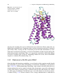
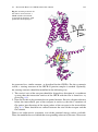
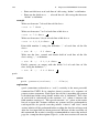
There is only small knowledge about the interaction between GPCR and G protein on molecular level available. Crystal structures of GPCRs (see Chap. 3 and
appendix Important Crystal Structures of GPCRs (Source: http://www.pdb.org)) on
the one hand and G proteins on the other hand are known (http://www.pdb.org). In
2008, a crystal structure of opsin cocrystallized with a part of the C-terminus of Gα
was published (Scheerer et al. 2008). In order to get a more detailed insight into
interactions between a GPCR and the Gα-subunit, in 2010, a hβ2 R-Gαs -complex
was predicted (Strasser et al. 2010). One year later 2011, a crystal structure of the
hβ2 R-Gαβγ -complex, which is shown in Fig. 2.7 was published (Rasmussen et al.
2011).
Fig. 2.7 Crystal structure of a hβ2 R-Gαβγ -Nb35-T4-Lysozyme complex. (Rasmussen et al. 2011)
G protein coupled receptors interact with heterotrimeric G proteins located in the
intracellular part of a cell, comprised of a Gα-subunit and a Gβγ heterodimer. If an
agonist binds to a GPCR, the GPCR undergoes a conformational change from the
inactive to the active state (Kobilka and Deupi 2007). In the active conformation, the
GPCR interacts with the appropriate G protein. Subsequently, the conformation of
the Gα-subunit changes by release of GDP and a GTP binds to the ternary complex,
10
2 G Protein Coupled Receptors
consisting of the agonist, the GPCR and the G protein. This leads to conformational
change of the Gα-subunit and the heterotrimeric G protein-complex dissociates into
a Gα-GTP- and a Gβγ-complex. In dependence of the subtype of the activated Gα
the appropriate signal cascades are induced selectively (Fig. 2.8) (Vauquelin and von
Mentzer 2007).
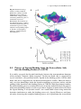
Fig. 2.8 Signalling cascade, induced by the binding of an agonist to a GPCR. Three different
signalling cascades with regard to Gαs , Gαi and Gαq are shown
2.4
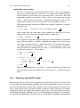
Important Internet Sources with Regard to GPCRs
A very important internet source is the “GPCR network” (http://cmpd.scripps.edu)
(Fig. 2.9). Here you can find important information concerning GPCRs. The “tracking status” of solving the crystal structure of distinct GPCRs might be of special
interest (see Chap. 3, Fig. 3.1).
2.4 Important Internet Sources with Regard to GPCRs
Fig. 2.9 Homepage of GPCR network. (http://cmpd.scripps.edu)
11
Chapter 3
Sequence Alignment and Homology Modelling
For molecular modeling of proteins in general, the structure of the protein is needed.
How can such a structure be obtained? One might consider first a modeling of the
protein structure de novo or ab initio based on the amino acid sequence. There are
several approaches described in literature (Fleishman et al. 2006; Yarov-Yarovoy
et al. 2006; Taylor et al. 2008; Zhang 2008; Barth et al. 2009; Zaki et al. 2010).
For small proteins, these techniques result in suitable structures, which are in good
accordance to experimentally derived structures. But it should be taken into account,
that with increasing number of amino acids, thus methods are not longer appropriate,
because of an exponentially increasing computational time. Thus, other techniques
are necessary. One is the technique of homology modelling. This is based on the
assumption that proteins of on class have a very similar structure. Thus, if the structure
of one protein of a distinct class is evaluated by experimental methods, the structures
of all other proteins can be modelled in homology to this experimental template. The
technique of homology modelling is used with regard to several GPCRs (Zhang et al.
2006), like the NK1 receptor (Evers et al. 2004), the P2Y6 receptor (Costanzi et al.
2005), the CB2 receptor (Pei et al. 2008), the NKB and NK3 receptor (Ganjiwale
et al. 2011), the cholecystokinin-1 receptor (Henin et al. 2006), histamine receptors
(Jongejan et al. 2005; Preuss et al. 2007; Jongejan et al. 2008; Lim et al. 2008;
Igel et al. 2009; Strasser and Wittmann 2010a; Brunskole et al. 2011) and besides
addresses GPCR oligomerization (Simpson et al. 2010).
3.1
Selection of a Template
To be able to start homology modelling, one has to search for an appropriate template
structure. A large number of such templates are available at the Protein Data Bank
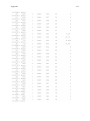
(PDB, http://www.pdb.org). Until end of 2011 a large number of crystal structures
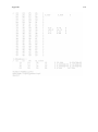
were available (Table 3.1). As illustrated by Table 3.1, most crystal structures concern the β1 - and β2 - adrenergic receptor. These crystal structures are of great interest,
since different types of ligands, like inverse agonists, antagonists or (partial) agonists
are bound. Thus, these crystal structures reveal important information with regard
A. Strasser, H.-J. Wittmann, Modelling of GPCRs,
DOI 10.1007/978-94-007-4596-4_3, © Springer Science+Business Media Dordrecht 2013
13
14
3 Sequence Alignment and Homology Modelling
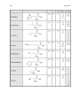
Table 3.1 pdb-codes of most important crystal structures related to opsin or GPCRs
GPCR
Related pdb-codes
Bovin (rhod)opsin
Human β2 adrenergic receptor
1F88, 1HZX, 1GZM, 3CAP, 3DQB, 3PQR, 3PXO
2RH1, 2R4R, 2R4S, 3D4S, 3NYA, 3NY8, 3NY9, 3KJ6,
3P0G, 3PDS, 3SN6
2VT4, 2YCW, 2YCX, 2YCY, 2YCZ, 2Y00, 2Y01,
2Y02, 2Y03, 2Y04
3PBL
3RZE
3ODU, 3OE6, 3OE8, 3OE9, 3OE0
3EML, 2YDO, 2YDV, 3QAK, 3PWH, 3REY, 3RFM
Turkey β1 adrenergic receptor
Human dopamine D3 receptor
Human histamine H1 receptor
Human chemokine CXCR4 receptor
Human adenosine A2A receptor
to different conformations of the receptors. Recently, the crystal structure of a ligand bound covalently to the hβ2 R was published (3PDS) (Rosenbaum et al. 2011).
Besides the crystal structures of adrenergic receptors, 2010 the crystal structure of
the human dopamine D3 receptor (3PBL) (Chien et al. 2010) and 2011 the crystal
strucuture of the human histamine H1 receptor (3RZE) (Shimamura et al. 2011) was
published. In addition to the mentioned crystal structures of biogenic amine receptors, crystal structures of the human chemokine CXCR4 receptor (Wu et al. 2010)
and the human adenosine A2A receptor (Jaakola et al. 2008; Lebon et al. 2011; Xu
et al. 2011; Dore et al. 2011) are known (Table 3.1).
Thus, if a GPCR has to be modelled an appropriate template has to be chosen.
If one likes to model a biogenic amine receptor by homology modelling, the crystal
structure of a biogenic amine receptor is suggested to be used as template to solve this
task. For modelling of inverse agonists or neutral antagonist in the receptor bound
state, a template, representing the inactive conformation should be chosen, whereas a
template, representing the active conformation should be used in case of (partial) agonists. Furthermore, the homology between the receptor to be modelled and the template should be as high, as possible. Based on these suggestions, it is the responsibility
of the modeller to choose an appropriate template for homology modelling.
Sometimes, a look onto the homepage of GPCR network (http://cmpd.scripps.
edu) is very useful. There, you get information about the tracking status of GPCRs
which will be crystallized in future (Fig. 3.1).
3.2
Crystal Structures of GPCRs (Source: http://www.pdb.org)
In the appendix, the most important information with regard to all crystal structures
of (rhod)opsin or GPCRs is summarized tabular. These tables should give you a fast
overview onto available crystal structures, resolution, structure of a cocrystallized
ligand, related UniProtKB entries and corresponding literature. Have a careful look
onto the section “mutation”! Often, not the wild type receptor is crystallized, instead
point mutations were introduced. Thus, if you want to model the receptor, which
is crystallized, you may change the amino acids, mutated in the crystal structure,
into the corresponding amino acid of the wild type receptor. An overview of the
differences in crystal structures is given by the Figs. 3.2–3.6.
www.allitebooks.com
3.2
Crystal Structures of GPCRs (Source: http://www.pdb.org)
15
Fig. 3.1 GPCR tracking status. (Status: November 2011; Source: http://gpcr.scripps.edu/tracking_
status.htm)
Fig. 3.2 Crystal structure
of the turkey β2 R, 2Y00.
(Warne et al. 2011)
16
3 Sequence Alignment and Homology Modelling
Fig. 3.3 Crystal structure of the human β2 R, 3PDS. (Rosenbaum et al. 2011)
Fig. 3.4 Crystal structure of
the human CXCR4, 3ODU.
(Wu et al. 2010)
3.2
Crystal Structures of GPCRs (Source: http://www.pdb.org)
Fig. 3.5 Crystal structure of
the human CXCR4, 3OE0.
(Wu et al. 2010)
Fig. 3.6 Crystal structure of
the human A2A R, 3EML.
(Jaakola et al. 2008)
17
18
3 Sequence Alignment and Homology Modelling
3.3 Amino Acid Sequences and Sequence Alignment
Before being able to start the homology modelling, it has to be decided which amino
acid of the template sequence corresponds to an amino acid in the target sequence.
Therefore, a sequence alignment has to be performed manually or automatically.
Clustal (http://www.clustal.org) for example, is a software for multiple sequence
alignment. However, before starting with sequence alignment, the corresponding
amino acid sequences have to be obtained.
3.3.1 Amino Acid Sequences – Where to Get From?
There are several sources for amino acid sequences present in the internet. One
prominent is for example the Expasy Proteomics Server (http://expasy.org) (Fig. 3.7).
Exercise Start your internet browser and open the site http://expasy.org. Now
choose “UniProtKB” under the section “query”. Then you can type your search
string into the field on the right.
Now we want to search for the human adrenergic β2 receptor. There are
different possibilities for the search string. For example, type “adrenergic” and
click the “Search” button. Now, more than 900 results, related to “adrenergic”
are presented. Scroll, until the receptor of your choice is listed. In our case it
is the human adrenergic β2 receptor with the accession code “P07550”. If you
want to reduce the number of hits, the search string has to be defined more
exactly. Please try “beta adrenergic receptor”, “beta-2 adrenergic receptor”
and “beta-2 adrenergic receptor human”. By defining the search string more
exactly, the number of hits can be significantly reduced and it is easier for you
to find the hit, you are searching for.
Now, click, onto the corresponding entry with the accession code “P07550”
and you get a lot of very useful information about this receptor, including the
amino acid sequence. In the section “Regions”, the amino acids, related with
the N-terminus, C-terminus, intracellular loops, extracellular loops and transmembrane domains are given. This information is very helpful for the sequence
alignment later on. In the section “Sequence” you can find the whole amino
acid sequence of the protein. For further proceeding on with the amio acid
sequence like for sequence alignment, it may be easier for you, to download
the amino acid sequence as “fasta” format. To do so, please click onto the
string “FASTA”. Now you get the amino acid sequence as simple ascii file.
Fig. 3.7 Homepage of the expasy server. (http://expasy.org)
3.3 Amino Acid Sequences and Sequence Alignment
19
20
3 Sequence Alignment and Homology Modelling
Table 3.2 Highly conserved amino acid according to Ballesteros (Ballesteros et al. 2001) of each
transmembrane domain of rhodopsin-like GPCRs
TM I
TM II
TM III
TM IV
TM V
TM VI
TM VII
Asn, N
Asp, D
Arg, R
Trp, W
Pro, P
Pro, P
Pro, P
3.3.2
Ballesteros Nomenclature
A careful analysis of the known amino acid sequences of known rhodopsin-like
GPCRs by Ballesteros (Ballesteros et al. 2001) exhibited the most conserved amino
acid within each of the seven transmembrane domains, which is used as a reference
for all other amino acids within the same helix. Within this nomenclature, the term
X.YY is used. Therein, X represents the number of the transmembrane domain and
YY the position of the residue within the transmembrane domain. The most conserved
amino acid within one helix gets the number 50. All other amino acids within the
same helix are numbered relative to that highly conserved position 50. The highly
conserved amino acids of each transmembrane domain of a GPCR, according to the
Ballesteros nomenclature (Ballesteros et al. 2001) are given in Table 3.2.
In Fig. 3.8, the complete amino acid sequence with the conserved amino acids
according to Ballesteros (Ballesteros et al. 2001) of the human adrenergic β2 receptor
is presented.
One should pay attention onto the transmembrane regions, as pointed out in
Fig. 3.8. As already mentioned the amino acids related to the transmembrane regions
are given at http://expasy.org under the corresponding accession code. A comparison
to the corresponding crystal structure – if available – shows sometimes differences
with regard to the helical region. Let us for example look onto TM III of the human
adrenergic β2 receptor. The transmembrane region is defined from Glu-107 until Val129 at expasy (Fig. 3.9a). However, a closer look onto the corresponding domain
at the crystal structure shows that the helical structure is much longer at both sides
(Fig. 3.9b). Thus, the domains are adopted with regard to the amino acid sequence
in Fig. 3.9c. Additionally, in Fig. 3.9b, the amio acids Glu-107 and Val-129 are mentioned Glu3.26 and Val3.48 in the Ballesteros nomenclature. Some additional amino
acids are shown in the Ballesteros nomenclature in Fig. 3.9c. For the termini and the
loops no corresponding nomenclature is available.
3.3.3 Amino Acid Sequences – Templates
Before performing an amino acid sequence alignment, one has to decide, which
structure should be used as template structure for homology modelling. Meanwhile
a lot of crystal structures of bovin rhodopsin or GPCRs like the human adrenergic β2 receptor or turkey adrenergic β1 receptor are available (see Tab. 3.1 and
appendix Important Crystal Structures of GPCRs (Source: http://www.pdb.org)). It
cannot be decided overall, which crystal structure should be used as a template for
3.3 Amino Acid Sequences and Sequence Alignment
21
Fig. 3.8 Amino acid sequence of the human adrenergic β2 receptor. The transmembrane domain
are presented, as defined at http://expasy.org, accession code P07550. The highly conserved amino
acids, defined by Ballesteros (Ballesteros et al. 2001) are marked by red boxes
Fig. 3.9 Helical structure of a transmembrane domain. a Definition of the TM domain III of the
human adrenergic β2 receptor at expasy (http://www.expasy.org). b TM III of the human adrenergic
β2 receptor of a crystal structure. c Amino acid sequence of TM domain III, based on the crystal
structure
22
3 Sequence Alignment and Homology Modelling
homology modelling. In general, the crystal structure with highest sequence homology to the receptor, which is intended be modelled, should be chosen. Besides that
it should be taken into account that different template crystal structures in homology
modelling could lead to differences in the resulting homology model. However, the
mainly used templates for modelling class A GPCRs are bovine rhodopsin and the
human adrenergic β2 receptor (see appendix Important Crystal Structures of GPCRs
(Source: http://www.pdb.org)).
3.3.4
Sequence Alignment
After retrieving the amino acid sequences of the template structure and the destination
receptor, the sequence alignment can be performed. There exist several techniques,
to perform the sequence alignment. On the one hand, the sequence alignment can be
performed manually. The corresponding steps require some time and concentration.
On the other hand, there exist several software products, which allow performing
an alignment automatically, like clustal (http://www.clustal.org) (see appendix Summary of Important Internet Resources). However, if software is used, it is definitely
necessary to check to resulting alignment in order to avoid unexpected mistakes or
some inaccuracies.
For a manual sequence alignment, the alignment is performed by several steps:
1. Use the information of the expasy server (http://expasy.org) to get an idea about
the amino acids of the seven transmembrane domains for template and target
sequence.
2. Perform the sequence alignment for each transmembrane domain in ascending order. Here, it is necessary, that the highly conserved amino acid of each
transmembrane domain has the same position in template and target.
3. Now, the alignment for the termini and loops can be performed. There you have
to take into account several points:
– In most crystal structures, the N-terminus and C-terminus are often not complete. Thus, there you can perform the alignment of such regions, but there is
no real use in homology modelling, since no template structure is given for
such regions.
– The I1-, E1-, I2- and E3-loop can be aligned easily in most cases to the template
sequence. However it should be taken into account, that corresponding loops
of different GPCRs could differ in their length. This has to be taken carefully
into account later on in the homology modelling. To declare a vacant position
in amino acid sequence, a hyphen (-) is used in general.
– The I3-loop differs significantly in length (from some ten to some hundred
amino acids) within the different GPCRs. Additionally, the I3-loop is not completely present in the crystal structures, available up to now. Thus, a complete
I3-loop alignment is useless for homology modelling. However, for MD simulations, it will be useful to close the open ends between TM V and TM VI.
3.4 Homology Modelling
23
Fig. 3.10 Manual alignment of the hH4 R to the hH1 R. green: termini and loops; grey: transmembrane domains; red boxes: highly conserved amino acids (Ballesteros et al. 2001); yellow: highly
conserved cysteine, establishing a disulfide bridge to the upper part of TM III; -: missing amino
acids; the amino acids of the I3-loop are not shown completely, which is indicated by dots
Therefore, some amino acids of the beginning and end of the I3-loop are
modelled correctly and the gap is closed by an alanine chain.
– The E2-loop has to be aligned very carefully. It has to be taken into account,
that there is a highly conserved disulfide bridge between the E2-loop and the
upper part of TM III. Thus, the corresponding cysteine has to be positioned
correctly.
An example for an alignment of the human histamine H4 receptor to the human
histamine H1 receptor is shown in Fig. 3.10.
3.4
3.4.1
Homology Modelling
Modelling of the Transmembrane Domains
The helical transmembrane domains can be easily modelled straight forward. Therefore, only the amino acid side chains have to be changed into the side chain of the
destination with appropriate modelling software.
3.4.2
Modelling of Loops
In general the transmembrane domains of different GPCRs consist of the same number of amino acids. Thus, the homology modelling of transmembrane domains is
quite easy and can be performed straight forward. In case of intra- or extracellular loops, which are connecting the transmembrane domains, differences in number
of amino acids of a loop between different GPCRs can occur. This is the case for
the E2- or E3-loop between hH1 R and hH4 R (Fig. 3.10). Small gaps can be closed
with “loop search” modules by using appropriate software. For some biogenic amine
24
3 Sequence Alignment and Homology Modelling
Fig. 3.11 Different conformations of the E2-loop based on crystal structures
receptors, an influence of extracellular loops, especially the E2-loop, onto the binding of ligands to the receptor was shown (Lim et al. 2008; Brunskole et al. 2011).
Thus, a correct modelling of the loops is very important. Most of the loops are resolved by crystal structures. However, this is often not the case with regard to the
extracellular loop E2 and this is not the case with regard to the intracellular loop I3.
Since the E2-loop is in contact with the binding pocket, the E2-loop has to be
modelled completely. If you look onto different crystal structures with complete
E2-loop, you can see different conformations (Fig. 3.11).
Thus, you have to decide carefully, which template is to be used for modelling
of the E2-loop. A large number of crystal structures are obtainable for the human
adrenergic hβ2 receptor. But the hβ2 R is a special case: There are two disulfide
bridges in the E2-loop (Fig. 3.12), whereas in most others GPCRs there is only one
disulfide bridge in the E2-loop, connecting the E2-loop with the upper part of the
TM III.
A part of the E2-loop of the hβ2 R exhibits a helical structure, but this is not the case
for all other GPCRs. Thus, you have to decide carefully, if it would be appropriate
to use two different template structures for homology modelling: one for the E2loop and one for the remaining parts of the receptor. However, the E2-loops are
widely different in their length, thus, in most cases, the E2-loop cannot be modelled
by changing an amino acid side chain of the template into the side chain of the
destination. Thus, you have to use also techniques, like “loop search”. For only one
loop search, the number of amino acids is too long, and you would get bad results.
Thus, it is better, to use at least one fixed point. This is the highly conserved cysteine,
connecting the E2-loop by a disulfide bridge with the upper part of TM III (Fig. 3.10).
www.allitebooks.com
3.4 Homology Modelling
25
Fig. 3.12 Different numbers of disulfide bridges in the E2-loop
3.4.3
Modelling of Internal Water
A detailed analysis of the crystal structures of GPCRs reveals that there are internal,
highly conserved water molecules present (Fig. 3.13). Several studies showed that
these water molecules are involved in the hydrogen bonding within the receptor.
Based on the published data, it can be suggested, that these water molecules are
essential for stabilizing the receptor or important for receptor activation (Pardo et al.
2007). Thus, in order to generate a stable receptor model, the water molecules which
are localized/crystallized within the receptor should be included into the homology
model.
3.4.4
Modelling of the C-Terminal Part of the Gα Subunit
or the Whole Gα Subunit
Based on several studies it is suggested, that a GPCR in its active conformation
interacts in the intracellular part with the Gα subunit. There is only small knowledge
about the receptor – G protein interaction. However, recently, the crystal structure of
opsin, cocrystallized with eleven amino acids of the C-terminus of the Gα subunit
(Scheerer et al. 2008) and a complete GPCR – G protein complex (Rasmussen et al.
2011) were published. A detailed analysis of the corresponding crystal structures
(3DQB, 3SN6) shows, that the C-terminus of the Gα subunit is deeply bound in a
pocket between the transmembrane domains. Leaving out this part of the Gα will
result in some problems in subsequent molecular dynamic simulations. In general, if
molecular dynamic simulations of a receptor are performed, the receptor is embedded
in its natural surrounding. Thus, if the C-terminal part of Gα or the whole Gα is
26
3 Sequence Alignment and Homology Modelling
Fig. 3.13 Crystal structure of
bovin rhodopsin (1GZM)
with internal water (red
balls). (Li et al. 2004)
missing, the resulting free space is filled with water molecules. Water molecules are
highly polar and thus have completely other (surface) properties than the C-terminal
part of Gα. Thus, leaving out the C-terminal part of Gα and substitution by water
molecules in molecular dynamics can lead to instabilities of the receptor during the
molecular dynamic simulation. Thus, it is suggested, to include at the whole Gα or
least the C-terminal part of Gα in a homology model. Be aware, that each GPCR
couples to a distinct Gα subunit (Fig. 2.8).
3.4.5
Refinement of the Receptor Model
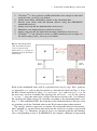
After finishing the homology modelling, several checks of the complete model should
be performed. A typical error of beginners in molecular modelling is presented in
Figs. 3.14–3.16. During homology modelling, some amino acid side chains have to
be mutated into the correct amino acid side chain. Sometimes, especially with regard
to long side chains or aromatic rings, collisions between the side chains arise. There
are two types of collisions: In the first type, two side chains are in close contact,
as shown in Fig. 3.14. In most of these cases, energy minimization is sufficient to
3.4 Homology Modelling
27
Fig. 3.14 Close contact between the atoms of a lysine and phenylalanine: Left: before minimization,
right: after minimization
Fig. 3.15 Part of a protein
structure after minimization.
What is the problem?
remove the collision and suitable structures might be obtained. The second type of
collision is a more difficult pitfall, which is illustrated in Figs. 3.15 and 3.16. Look
carefully onto the Fig. 3.15. Where is the problem?
After a careful look onto the picture you may see, that there is a problem with
regard to a lysine and phenylalanine in box B3. This is also illustrated in Fig. 3.16.
Here, a long amino acid side chain, like present in lysine, is located within
an aromatic ring, like present in tyrosine, phenylalanine, tryptophane or histidine.
28
3 Sequence Alignment and Homology Modelling
Fig. 3.16 Wrong close contact between the atoms of a lysine and phenylalanine: Left: before
minimization, right: wrong structure after minimization
Unfortunately, a large number of modelling software minimizes a protein, containing
such type of wrong structure. And additionally in most cases the potential energy is
negative. Thus, one might conclude that all is well. However, often during molecular
dynamic simulation, problems occur and the simulation stops with an error. If this
is the case, you have to go back to your starting structure and look for the error.
Often, an error, similar to that described above (Fig. 3.16) causes the problem. A
similar problem can occur not only within the protein, but also between protein
and lipid molecules. If there are collisions between amino acid side chains, one
has to decide, how to remove this collisions. In general, there are two possibilities:
First, one can simply perform an energy minimization. But in some cases, this could
lead to artefacts, especially, if two aromatic moieties are linked together. Thus, it
is suggested, that one looks separately onto each collision and tries to remove the
collisions by carefully changing the corresponding dihedral angles.
After completing these steps, the homology model can be energetically minimized.
Here it is suggested, that the energy minimization is performed step by step. In
order to avoid structural artefacts, induced by minimization, it is important, that
the backbone of the transmembrane domains is provided with position restraints
during a first minimization. In a subsequent minimization steps, the receptor can be
minimized without any position restraints. Afterwards, the model should be checked,
addressing the following items and if everything is correct, one can start with further
modelling studies, like docking or molecular dynamic simulations.
Check for the correct amino acid sequence
Check for the presence of the disulfide bridge between the E2-loop and
the upper part of TM III
Check for the correct configuration of the amino acids
Check for collisions or bad contacts between amino acid side chains
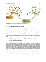
Chapter 4
Construction of Ligands
Some molecular modelling software include very comfortable editors, which allow to construct ligands. Additionally, distinct atom types can be assigned to these
atoms. In contrast, Gromacs (http://www.gromacs.org) is a powerful software package for molecular dynamic simulations and no editor for construction of ligands is
included. Therefore, we recommend that you download an appropriate editor, like
chimera (http://www.cgl.ucsf.edu/chimera/) and install this on your computer. In
general, you can also use other software to construct your 3D-molecules, but the
software should be able to save the molecule as pdb-file. Before you can use Gromacs (http://www.gromacs.org) to simulate organic compounds, like a ligand, you
have to generate a topology-file of the molecule of interest. In general, your molecule
editor is not able to create an appropriate topology-file. We do not recommend constructing a topology-file manually, because therefore you need detailed knowledge
about types of the atoms or sites and their force field parameters on the one hand.
On the other hand, you have to define bonds, angles and dihedrals, which is a very
complicated procedure for a beginner. Besides, generating a topology file manually,
is very susceptible for mistakes. Solving this task, you can use the PRODRG-server
(http://davapc1.bioch.dundee.ac.uk/prodrg/). The starting page of the server is shown
in Fig. 4.1.
If you have started the PRODRG server (http://davapc1.bioch.dundee.ac.uk/
prodrg/), use the button “Run PRODRG”, which will bring up the next page (Fig. 4.2):
The academic use of the PRODRG server is free, but in order to avoid abuse, one
user is allowed to perform about three runs per day. Therefore, you have to order
a so-called “token” by submitting your e-mail address. Within some minutes, you
should get your “token”. Now copy and paste your valid “token” into the appropriate
field. Afterwards, you can fill the remaining fields and submit your PRODRG job.
For obtaining the GROMACS coordinate and topology-file of ethanol for example,
start a molecule editor, like chimera, construct ethanol and save the molecule as
pdb-file, named ethanol.pdb.
A. Strasser, H.-J. Wittmann, Modelling of GPCRs,
DOI 10.1007/978-94-007-4596-4_4, © Springer Science+Business Media Dordrecht 2013
29
30
4 Construction of Ligands
Fig. 4.1 Homepage of the PRODRG server. (http://davapc1.bioch.dundee.ac.uk/prodrg/)
Fig. 4.2 Site for compound submission of the PRODRG-server
Construction of Ligands
HEADER
COMPND
REMARK
HETATM
HETATM
HETATM
HETATM
HETATM
HETATM
HETATM
HETATM
HETATM
CONECT
CONECT
CONECT
CONECT
CONECT
CONECT
CONECT
CONECT
CONECT
MASTER
END
ETHANOL
ETHANOL
GENERATED
1 O2 LIG
2 H3 LIG
3 C1 LIG
4 H2 LIG
5 H1 LIG
6 C4 LIG
7 H6 LIG
8 H5 LIG
9 H4 LIG
1
2
3
2
1
3
1
4
4
3
5
3
6
3
7
7
6
8
6
9
6
0
0
0
31
BY
1
1
1
1
1
1
1
1
1
SYBYL (TRIPOS, INC.) 15-AUG-10
-8.207 3.565 -0.317 1.00 -0.40
-7.452 3.455 0.253 1.00 0.21
-9.325 2.747 0.067 1.00 0.04
-9.665 3.010 1.084 1.00 0.06
-10.148 2.959 -0.635 1.00 0.06
-8.958 1.244 -0.007 1.00 -0.04
-8.620 0.992 -1.024 1.00 0.03
-8.149 1.012 0.702 1.00 0.03
-9.834 0.624 0.241 1.00 0.03
5 6
8 9
0
0
0
0
0
9
0
9
0
Open the file ethanol.pdb with an editor, copy all data and paste them into the
appropriate field of the PRODRG-site, shown in Fig. 4.2. Since ethanol is not chiral,
you can choose “no” at the corresponding field. Additionally choose “full charges”
and “yes” with regard to EM (EM means energy minimization). Afterwards, click
at the button “Run PRODRG”. After some minutes, you obtain the results-page. At
first, you see some remarks of the server and additionally, the molecule with (added)
hydrogens is shown (Fig. 4.3).
If your scroll down, you see a summary of different output-files (Fig. 4.4). Most
important, concerning GROMACS is the third item under “Coordinates” and the first
item under “Docking/MD simulations”.
Within the “Coordinates” section for GROMACS, you find three different items,
namely a coordinate file with “polar hydrogens”, with “polar/aromatic hydrogens”
and with “all hydrogens”. If you look onto the number of coordinate lines you see
differences, in case of ethanol, between “polar hydrogens” and “all hydrogens”.
Since the site-concept is used in GROMACS, the hydrogens of an alkyl-moiety are
integrated within the carbon. This means for example, that a methyl group (CH3 ) does
not consist of four sites – one carbon and three hydrogens – instead, it is summarized
in one site (see Chap. 9). This is a very important aspect with regard to simulation
time. Because of the combination of several atoms to one site, the number of sites is
reduced and this leads to an exponential decrease in simulation time. If you compare
with the contents of the topology-file, the coordinate file “polar/aromatic” hydrogens
is relevant. Be aware, that the number of coordinates in the gro-file (Fig. 4.5) has
32
Fig. 4.3 First part of the results-page of the PRODRG-Server
Fig. 4.4 Overview of different outputs of the PRODRG server
4 Construction of Ligands
Construction of Ligands
33
Fig. 4.5 Three different GROMOS87/GROMACS coordinate files as output of the PRODRUG run
to be the same as in the topology file. Thus, copy all lines within the box titled
“polar/aromatic hydrogens” and save them in a file named ethanol.gro.
Now, scroll down to the section “The GROMACS topology” (Fig. 4.6), copy the
contents and save in a file named ethanol.itp.
Now, you have all data for performing simulations including ethanol with
GROMACS.
In the following box, a summary of all steps for generating a GROMACS
coordinate- and topology-file is given:
34
4 Construction of Ligands
Fig. 4.6 GROMACS-topology-file of ethanol, calculated by the PRODRG server
www.allitebooks.com
Construction of Ligands
35
Construct your ligand with an appropriate editor as 3D-structure
Check your molecule, if e.g. the configuration of chiral atoms is correct
Minimize your molecule, if possible
Save the minimized molecule as pdb-file
Start the PRODRG-Server
If you do not have a token to work with the PRODRG-Server, please, fill
in your E-Mail in the corresponding field and used the “Send” button. Be
aware, that it may take some time, before you get your token via E-Mail
If you have the token, please copy it from your E-Mail into the appropriate
field. Now, you can start working with PRODRG.
Open your pdb-file in an appropriate editor
Copy and paste the whole pdb-file into the corresponding field of the
PRODRG-server
Choose “Yes” or “No” in the field chirality (depends on your molecule)
Always choose “full charges” in the field charges
Choose “Yes” in the field EM (energy minimization)
Now, start your PRODRG-Job. Please be aware, that the calculations may
take a while and do not close your browser
Copy your GROMACS coordinates with polar/aromatic hydrogens and
save them as gro-file
Copy your GROMACS topology and save it as itp-file
Load your gromacs-coordinate file into an editor for visualization of
molecules and verify the structure
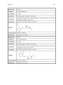
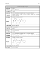
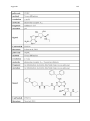
Next, we present another example, dealing with the ligand dobutamin (Fig. 4.7).
Fig. 4.7 Structure of
dobutamine (only R
enantiomer shown),
cocrystallized with the turkey
β1 adrenergic receptor in the
crystal structure 2Y00.
(Warne et al. 2011)
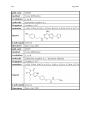
Dobutamine is a β1 -sympathomimetic drug. It is cocrystallized with the turkey
β1 adrenergic receptor in the crystal structure 2Y00 (Warne et al. 2011).
36
4 Construction of Ligands
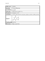
Exercise Please upload the dobutamine in its neutral form, as pointed out in
Fig. 4.7 to the PRODRG-server and create the appropriate files, as mentioned
above. If you have done so, you should have a closer look onto the output
of the PRODRG-server (Fig. 4.8). You can see, that now the dobutamine is
positively charged, since there is an additional hydrogen at the amino moiety.
Remember, you uploaded dobutamine in its neutral form. Be aware, that this
is typical for the PRODRG-server: molecules with a basic or acid moiety are
calculated in its charged form.
Fig. 4.8 Output of the PRODRG-Server with regard to dobutamine
The action, that molecules with a basic or acid moiety are calculated in its charged
form, is based on the behaviour of carboxylic acid or amines in water at pH values
about 7. Under these conditions, carboxylic moieties for example are deprotonated,
and amino moieties are protonated.
Chapter 5
Lipids
Lipid membranes separate two compartimentes from each other: they separate a cell
from the surrounding, or they separate the cytoplasm of cells into organelles. These
membranes consist of two layers of lipid, the so called lipid bilayer. The lipid bilayer
is a planar, two dimensional fluid.
A large number of proteins belong to the class of membrane proteins. Membrane
proteins can be divided into two groups: First, peripheral membrane proteins, which
are located on the surface of the lipid bilayer and second, the integral membrane
proteins. It is typical for integral membrane proteins, that they are embedded into the
phospholipid bilayer. GPCRs belong to the membrane proteins and are also called
7TM receptors, since they consist of 7 transmembrane domains, which cross the
lipid bilayer. These transmembrane domains are connected by sections with some
few up to some hundreds of amino acids, which are located in the aequeous extraand intracellular sides of the lipid bilayer.
Within the first molecular modelling studies of GPCRs, the GPCRs were modelled in the gas phase. This was a very rigorous approximation, because, the amino
acid side chains, pointing outwards of the receptor, were not in contact with the native surrounding. This could lead to incorrect amino acid side chain conformations,
or to artificial interactions between polar or charged amino acids. Additionally, if
molecular dynamic simulations were performed of a GPCR in the gas phase, the
secondary and tertiary structure of the receptor was not stable. In order to achieve
stability, constraints had to be put onto the backbone of the protein. Thus, conformational changes with regard to the whole receptor could not be observed. But with
the development of more efficient computers, it was possible to simulate GPCRs in
their natural surrounding, like lipid bilayer including intra- and extracellular water.
Meanwhile, it is widespread established, to model a GPCR in its natural surrounding.
5.1
Structure of Lipids
Lipids can be divided into several groups, the phosphoglycerides, sterols, sphingolipids, triglycerides and glycolipids. Membrane bilayers are mainly constituted
by phosphoglycerides. A schematic representation of phophoglycerides is given in
Fig. 5.1.
A. Strasser, H.-J. Wittmann, Modelling of GPCRs,
DOI 10.1007/978-94-007-4596-4_5, © Springer Science+Business Media Dordrecht 2013
37
38
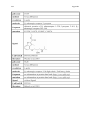
5 Lipids
Fig. 5.1 Structure of phosphoglycerides
The phosphoglycerides are established by one glycerol. Two long-chain fatty
acids are esterified to the carbons C1 and C2 of the glycerol. The fatty acids are
carboxylic acids with about 12–20 carbon atoms. A phosphoric acid is esterified to
C3 of the glycerol and an alcohol to the phosphate. Due to their chemical structure,
phosphoglycerides are amphiphilic. The head groups are hydrophilic, whereas the
long fatty acids show hydrophobic properties. In biological systems, a large variety
of phosphoglycerids is found, since there is a high variability with regard to the
alcoholic group and the fatty acids.
The name of the phosphoglycerides is based on the alcoholic head groups:
•
•
•
•
•
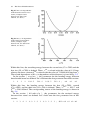
•
Phosphatidic acid, PA (no head group), i.e. POPA
Phosphatidylcholine, PC, i.e. POPC
Phosphatidylethanolamine, PE, i.e. POPE
Phosphatidylglycerol, PG, i.e. POPG
Phosphatidylinositol, PI
Phosphatidylserine, PS, i.e. POPS
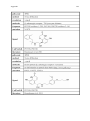
The PO in the lipids mentioned above, is the abbreviation for 1-palmitoyl-2-oleol.
For MD simulations, GPCRs are mainly embedded into POPC lipid bilayers (Ivanov
et al. 2005; Filizola et al. 2006; Henin et al. 2006; Strasser et al. 2007). The structure
5.2 Structure of the Phospholipid Bilayer
39
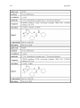
of POPC is presented in Fig. 5.2. However, other lipid models, like DOPC
(dioleoylphosphatidylcholine) are used (Goetz et al. 2011).
Fig. 5.2 Structure of POPC (1-palmitoyl-2-oleoylphosphatidylcholine)
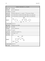
Sterols are another important class of membrane lipids. One of the most prominent
is the cholesterol (Fig. 5.3). The cholesterol scaffold contains four condensed rings
leading to a distinct rigidity. This structure is hydrophobic and thus it is able to insert
into the hydrophobic inner layer of the lipid bilayer. The polar hydroxyl moiety is
located at the surface of the lipid bilayer.
Fig. 5.3 Structure of
cholesterol
Cholesterol is sometimes found cocrystallized in combination with crystal structures of GPCRs. For example, a cholesterol specific binding site was identified for
the human β2 adrenergic receptor within the crystal structure 3D4S (Hanson et al.
2008).
5.2
Structure of the Phospholipid Bilayer
In Fig. 5.4, a site model of a lipid bilayer is presented. The hydrophobic chains
point inside the lipid bilayer, whereas the polar head groups are facing towards the
surrounding water.
40
5 Lipids
Fig. 5.4 Model of a lipid
bilayer with water on both
sides
5.3
Lipid Bilayer Models Used in Molecular Modelling
Several lipid models were constructed for use in molecular modelling. Some of them
are summarized in Table 5.1.
Table 5.1 Summary of some DPPC
lipids, often used in molecular DMPC
modelling studies
DOPC
POPC
POPE
PLPC
5.4
Dipalmitoylphosphatidylcholine
Dimyristoylphosphatidylcholine
Dioleoylphosphatidylcholine
1-palmitoyl-2-oleoylphosphatidylcholine
1-palmitoyl-2-oleoylphosphatidylethanolamine
Palmitoyllinoleylphosphatidylcholine
Internet Sources for Lipid Bilayer Models
In the internet, there are some sources which give a more detailed information with
regard to lipid bilayers, including simulation parameters for GROMACS. At some
sites in internet, equilibrated lipid bilayer models can be obtained via free download.
A summary of the most important internet resources with regard to lipids is given in
Table 5.2.
Table 5.2 Most important
internet resources with regard
to lipds
URL
http://lipidbook.bioch.ox.ac.uk
http://moose.bio.ucalgary.ca/index.php?page=Structures_and_
Topologies
http://www.lrz-muenchen.de/∼heller/membrane/membrane.html
http://www.scmbb.ulb.ac.be/Users/lensink/lipid/
A very comfortable site is lipidbook (http://lipidbook.bioch.ox.ac.uk) (Domanski
et al. 2010). The aim of the lipidbook is “a public repository for force field parameters
with special emphasis on lipids” (http://lipidbook.bioch.ox.ac.uk) (Fig. 5.5). Here,
you can individually select the force-field, the parameter notation for distinct software
and the kind of lipid (Fig. 5.6).
5.4 Internet Sources for Lipid Bilayer Models
Fig. 5.5 Starting page of lipidbook (http://lipidbook.bioch.ox.ac.uk). (Domanski et al. 2010)
Fig. 5.6 Browser in lipidbook (http://lipidbook.bioch.ox.ac.uk). (Domanski et al. 2010)
41
42
5.5
5 Lipids
Embedding a GPCR into a Lipid Bilayer
For embedding a GPCR into a lipid bilayer, different strategies are available. The
most time consuming would be to simulate the whole system de novo, by putting an
appropriate number of lipid and water molecules randomly around the GPCR and
start a molecular dynamics simulation. Since this procedure is really time consuming,
alternative methods are suggested: One approach could be to set an appropriate number of lipid molecules in appropriate orientation around the protein (Woolf and Roux
1996; Belohorcova et al. 1997). However, for this strategy, you must have access to an
appropriate software, or you have to establish the software by yourself. Alternatively,
for setting up your simulation box, you can start with already prepared lipid bilayers.
Therefore, you can look at the mentioned internet resources (Table 5.2), download an
equilibrated lipid bilayer model and use this for further calculations. Alternatively,
you can construct a lipid bilayer individually with a distinct width with an appropriate software. One suitable software is vmd (http://www.ks.uiuc.edu/Research/vmd/),
combined with some scripts, as described in more detail later on. The great advantage
of the latter strategy is that you can individually adopt the size of your lipid bilayer
with regard to the size of the GPCR or the GPCR-Gαβγ-complex. In this context
you have to take into account two considerations: What do you want to simulate:
Only a GPCR or a whole GPCR-Gαβγ-complex. Due to the larger size of a GPCRGαβγ-complex, compared to a GPCR, the lipid bilayer has to be large in case of
a GPCR-Gαβγ-complex. However, in both cases, the lipid bilayer must be large
enough in order to guarantee that the GPCR or GPCR-Gαβγ-complex is embedded well. This means, you should have a lipid bilayer with a width of optimally
1.0–1.5 nm around your protein. This guarantees that there are not undesirable interactions between proteins of virtual simulation boxes as a result of periodic boundary
conditions, as illustrated in Fig. 5.7.
A lipid bilayer shell larger than 1.5 nm can be principally used, but this would not
lead to any advantage, instead, the great disadvantage will be an exponential increase
in simulation time. For simulation of a GPCR without the G protein, a width of the
lipid bilayer of about 9–10 nm is recommended. Thus, in the first step you have to
generate your lipid bilayer with an appropriate width (Fig. 5.8, step 1).
Subsequently, the GPCR has to be aligned into the lipid bilayer. A very
good description in combination with the software vmd (http://www.ks.uiuc.edu/
Research/vmd/) is found at the following internet site: http://www.ks.uiuc.edu/
Research/vmd/plugins/membrane/. A detailed description is given at the mentioned
site. However, in the following, a short description of a slightly modified procedure
using the script combine.tcl, available at (http://www.ks.uiuc.edu/Research/
vmd/plugins/membrane/) is presented. For the following procedure you need the
shell script vmd2gro, which is shown later on. The script vmd2gro was tested in
combination with vmd 1.8.7. Be aware, that in the presented version of vmd2gro
the POPC molecules in vmd-notation are transferd into the POPC-notation used by
Moose (http://moose.bio.ucalgary.ca/index.php?page=Structures_and_Topologies).
Thus, for further use with GROMACS, you need the files lipid.itp and
popc.itp. Both are available at http://moose.bio.ucalgary.ca/index.php?page=
5.5 Embedding a GPCR into a Lipid Bilayer
43
Fig. 5.7 Artificial close contacts of the protein in the simulation box with the proteins in the
neighboured virtual simulation boxes due to periodic boundary conditions
Structures_and_Topologies and can also be found in the appendix (POPC Parameters). In the script vmd2gro the tcl-script combine.tcl, developed by Balabin
and published at http://www.ks.uiuc.edu/Research/vmd/plugins/membrane/ was
used (see lines 192–276 in vmd2gro shown below). Before starting, you need your
protein as a correct pdb-file, which can be used as an input file for the GROMACS
command pdb2gmx without special options. In this example, this file is named
protein.pdb. In the next step, you can start vmd to generate the lipid bilayer.
Therefore, choose in the main menu Extentions → Modelling → Membrane
Builder. There, choose POPC as lipid, because the script vmd2gro only considers POPC in the version presented here. Define the length of the lipid bilayer in xand y-direction. Be aware to define the values in Å. In the actual version of the
script vmd2gro a box size of about (10 × 10 × 10) nm is defined (see line 188).
44
5 Lipids
Fig. 5.8 Step 1: Generate or
download a lipid bilayer of
appropriate size
However you can change the values in the script of later on in the gro-file, if necessary. So, for example type 100 for width in x- and y-direction in the appropriate
field of vmd. As “ouput prefix” type membrane. Subsequently, the membrane is generated and is shown in vmd. Additionally, in the directory, where vmd
is started from, two files, named membrane.pdb and membrane.psf are generated. The extension psf means “protein structure file”. In the next
step, the file protein.pdb has to be loaded via File → New Molecule. To
simplify the alignment of the protein in the lipid bilayer, use the menu Graphics
→ Representations → “Coloring Method → Color ID → yellow”
and “Drawing Method → New Cartoon”. Now, the coordinates of the protein have to be changed via Mouse → Move → Molecule. Be careful and move
ONLY the protein and NOT the membrane. Moving the membrane in the “move”
mode would result in a failure of the alignment! In the “move” mode, use the left
mouse button for translation, the shift-button and the left mouse button for rotation
around the z-axis and the shift-button in combination with the middle mouse button
to rotate around the axis vertical to the screen. Therefore, click directly onto the
protein with the mouse cursor. To leave the “move” mode, type “r” or use the
menu button Mouse → Rotate. In the “rotate” mode, you can rotate the whole
system (membrane and protein) as appropriate without changing any coordinates.
In the next step, you have to use the “move” and “rotate” mode alternately to
align the protein into the lipid bilayer. This procedure should be performed very
carefully with regard to the placement of the GPCR in the membrane. Additionally, this procedure needs some practice and may take some time. If the
www.allitebooks.com
5.5 Embedding a GPCR into a Lipid Bilayer
45
alignment procedure is finished, the protein with the new coordinates has to
be saved as pdb- and psf-file in the following manner: Use the menu buttons Extensions → Modelling → Automatic PSF Builder and a
new window, opens: Step 1: In the field “Output basename”, we write
protein_autopsf for example and click onto the button “Load input
files”. Step 2: Choose “Everything” and click onto “Guess and split
chains using current selections”. Step 3: Click onto “Create
chains”. Step 4: Click onto “Apply patches and finish PSF/
PDB”. An additional window opens, there, click “OK” and finish by clicking onto
the button “Reset Autopsf”. If you look into the directory, where vmd is started
from, three new files protein_autopsf.log, protein_autopsf.pdb and
protein_autopsf.psf are generated by the procedure, mentioned above. Now,
vmd can be closed and the shell script vmd2gro can be startet:
> vmd2gro
Subsequently, you have to define some basenames of files:
> Basename of membrane file: membrane
> Basename of aligned protein file: protein_autopsf
> Basename of output file (protein + membrane): temp
The first two basenames have to be the same as used in the alignment procedure
mentioned above. The third can have any basename, since these will be temporary
files, which will be deleted automatically.
After that, the script performs some calculations and then it stops in order to ask
you, if protonation states of amino acids should be changed. Here answer “no” by
typing a “n”. Subsequently, the command pdb2gmx is called within vmd2gro
and you are asked to choose an appropriate force-field. For example, type “4”.
Now, vmd2gro performs some time-consuming calculations, like generation of
a topology file. After some minutes, vmd2gro should have finished. Now, you
should have some new files in your current working directory: membrane.gro,
protein_autopsf.gro, protein_autopsf.gro, protein_autopsf.
top and posre.itp. The files membrane.gro and protein_autopsf.gro
contain the coordinates, relevant for the further steps. In membrane.gro,
the POPC-lipid-bilayer with a hole and in an appropriate site-notation is
given. Be aware, that the POPC in this notation can only be used with the
parameters available in internet (http://moose.bio. ucalgary.ca/index.php?page=
Structures_and_Topologies) and shown explicitly in the appendix (POPC Parameters). The file protein_autopsf.gro contains the coordinates of the
aligned protein and the file protein_autopsf.top is the corresponding
topology-file. The coordinates of both gro-files, membrane.gro and protein_
autopsf.gro can be combined within one gro-file, containing now the protein
and lipids. To do so, one can use the following LINUX-command-sequence:
46
5 Lipids
> set nr_prot = ‘wc -l protein_autopsf.gro |
cut -d’ ’ -f1‘
> set nr_mem = ‘wc -l membrane.gro | cut -d’ ’ -f1‘
> @ all_sites = ${nr_prot} + ${nr_mem} - 6
> echo "Protein in lipid bilayer" > prot_lip.gro
> echo "$all_sites" >> prot_lip.gro
> tail -n +3 protein_autopsf.gro |
head -n -1 >> prot_lip.gro
> tail -n +3 membrane.gro >> protein_lip.gro
Now, you should have your protein and the lipid bilayer in the file
protein_lip.gro. Of course, you can do the analogue manipulations manually with an editor. In protein_lip.gro, the lipid sites start again with number
1. To obtain a subsequent numbering and centring the structure in the simulation
box, use the GROMACS command editconf:
> editconf –f protein_lip.gro -c –o system.gro
The user of vmd2gro and the tcl-script combine.tcl developed by Balabin and published at http://www.ks.uiuc.edu/Research/vmd/plugins/membrane/
(see lines 192–276 in vmd2gro shown below) should add the absolute path for
top_all27_prot_lipid.inp in line 207. The script vmd2gro is shown in
the following:
1 #!/bin/tcsh
2
3 # vmd2gro: tcsh script to convert vmd format to
gro format
4 # for a lipid membrane/protein complex
5
6 # Detect and remove collisions between protein and
membrane using a Tcl script for VMD
7 # script statements follow a line beginning with
the the pattern "# START_TCL"
8
9 # Variables containing file names: mem, prot, out
10 # Tcl scriptfile "out.tcl" will be created on the
fly
11
12 echo -n "Basename of membrane file: "
13 set mem = "$ <"
14
15 if (! -e "${mem}.pdb") then
16
echo "Missing pdb file: ${mem}.pdb"
17
exit 1
18 else if (! -e "${mem}.psf") then
19
echo "Missing psf file: ${mem}.psf"
20
exit 1
5.5 Embedding a GPCR into a Lipid Bilayer
21
22
23
24
25
26
27
28
29
30
31
32
33
34
endif
echo -n "Basename of aligned protein file: "
set prot = "$ <"
if (! -e "${prot}.pdb") then
echo "Missing pdb file: ${prot}.pdb"
exit 1
else if (! -e "${prot}.psf") then
echo "Missing psf file: ${prot}.psf"
exit 1
endif
echo -n "Basename of output file (protein +
membrane): "
35 set out = "$ <"
36
37 if (-e "${out}.pdb") then
38
echo "File ${out}.pdb exists!"
39
echo "Rename existing file or choose new
file name and start again"
40
exit 1
41 else if (-e "${out}.psf") then
42 echo "File ${out}.psf exists!"
43 echo "Rename existing file or choose new
file name and start again"
44
exit 1
45 endif
46
47 # Create and start tcl script: out.tcl
48
49 if (-e "${out}.tcl") then
50 echo "Tcl script file ${out}.tcl exists!
Remove or rename it!"
51
exit 1
52 endif
53
54 # Substitutions for MEM, PROT and OUT in Tcl
script part
55
56 set begin_tcl = ‘grep -n "∧ # START_TCL" $0|
cut -d ':' -f1‘
57 echo $begin_tcl
58
59 tail -n +$begin_tcl $0|sed -e "s/MEM/$mem/"
47
48
5 Lipids
-e "s/PROT/$prot/" -e "s/OUT/$out/"
> "${out}.tcl"
60
61 if ("$status") then
62 echo "Error creating Tcl script file
${out}.tcl! Terminating!"
63 exit 1
64 endif
65
66 # Starting Tcl script from working directory!
67
68 chmod u + x "${out}.tcl"
69
70 vmd -e ${out}.tcl -dispdev text
71
72 if ("$status") then
73
echo "${out}.tcl failed! Terminating
calculations!"
74 exit 1
75 endif
76
77 echo "Output files ${out}.pdb and ${out}.psf
successfully created!"
78
79 echo "Going to convert pdb format to gro format"
80
81 # Removing obsolete files: pdb and psf files
of membrane and protein; tcl script file;
output psf file
82
83 rm "${mem}".{pdb, psf} "${prot}".{pdb, psf}
84 "${out}".tcl "${out}".psf
85
86 # Extracting protein and membrane structures
from out (*.pdb) file, deleting all water
molecules
87
88 grep 'POPC' "${out}.pdb" > "${mem}.pdb"
89 grep -v ’TIP\ | POPC’ "${out}.pdb"|grep 'ATOM'|
sed -e ’s/HSD/HIS/’ > "${prot}.pdb"
90
91 rm "${out}.pdb"
92
93 # Converting pdb file for protein and possibly
change protonation state
5.5 Embedding a GPCR into a Lipid Bilayer
94
95 echo "********************************************
*************************************************"
96 echo -n "Do you want to modify the protonation
state of amino acid ARG, ASP, GLU, HIS or LYS?
(y/n): "
97 echo "********************************************
*************************************************"
98
99 set answer = "$ < "
100 set answer = ‘echo $answer|tr 'y' 'Y'‘
101
102 set ARG = ""
103 set ASP = ""
104 set GLU = ""
105 set HIS = ""
106 set LYS = ""
107
108 if ("$answer" = = "Y") then
109
echo -n "Change protonation state of
ARG? (y/n): "
110 set h = "$ < "
111 set h = ‘echo $h|tr 'y' 'Y'‘
112 if ("$h" = = "Y") then
113
set ARG = "-arg"
114 endif
115
116 echo -n "Change protonation state of ASP? (y/n): "
117 set h = "$ < "
118 set h = ‘echo $h|tr 'y' 'Y'‘
119 if ("$h" = = "Y") then
120
set ASP = "-asp"
121 endif
122
123 echo -n "Change protonation state of GLU? (y/n): "
124 set h = "$ < "
125 set h = ‘echo $h|tr 'y' 'Y'‘
126 if ("$h" = = "Y") then
127
set GLU = "-glu"
128 endif
129
130 echo -n "Change protonation state of HIS? (y/n): "
131 set h = "$ < "
132 set h = ‘echo $h|tr 'y' 'Y'‘
133 if ("$h" = = "Y") then
49
50
134
135
136
137
138
139
140
141
142
143
144
145
5 Lipids
set HIS = "-his"
endif
echo -n "Change protonation state of LYS? (y/n): "
set h = "$ < "
set h = ‘echo $h|tr 'y' 'Y'‘
if ("$h" = = "Y") then
set LYS = "-lys"
endif
endif
pdb2gmx -f "${prot}.pdb" -o "${prot}.gro"
-p "${prot}.top" -ignh $ARG $ASP $GLU
$HIS $LYS
146
147 rm "${prot}.pdb"
148
149 # Converting pdb file for membrane ******
*****************************************
150
151 setenv LC_NUMERIC '.'
152
153 # Initializations -map VMD atomic numbers to
GRO atomic numbers (index)
154
155 set map = (4 3 5 1 2 17 23 20 21 22 24 25 28 30
31 32 33 45 48 51 54 57 60 63 65 67 70 73 76 79
82 36 39 40 41 42 92 95 98 101 104 107 110 113
116 119 122 125 128 131 85 88)
156
157 set gro_label = (C1 C2 C3 N4 C5 C6 O7 P8 O9 O10
O11 C12 C13 O14 C15 O16 C17 C18 C19 C20 C21 C22
C23 C24 C25 C26 C27 C28 C29 C30 C31 C32 O33 C34
O35 C36 C37 C38 C39 C40 C41 C42 C43 C44 C45 C46
C47 C48 C49 C50 CA1 CA2)
158
159 set n_gro = $#map # number of sites per lipid
molecule in gro notation
160 set n_pdb = 134 # number of
atoms per lipid molecule in VMD notation
161
162 set gro_file = "${mem}.gro"
163
164 # Caluclations and mapping
165
5.5 Embedding a GPCR into a Lipid Bilayer
51
166 @ units = ’wc -l "${mem}.pdb" | cut -d ' ' -f1’ /
$n_pdb # number of lipid molecules
167 @ number_of_atoms = $units * $n_gro
168
169 echo "Lipid membrane" >> $gro_file
170 echo "$number_of_atoms" >> $gro_file
171
172 set unit = 1
173 set atom_no = 1
174 while ("$unit" < = "$units")
175
set n = 1
176
@ i1 = ($unit - 1) * $n_pdb
177
while ("$n" < = "$n_gro")
178
@ pdb_line = $i1 + $map[$n]
179
180
gawk -v u = $unit -v line = $pdb_line
-v atom = $atom_no -v label = $gro_label[$n]
’NR = = line {printf("%5i%3s%7s%5i%8.3f%8.3f%8.3f\n",
u,"POP",label, atom,$6/10.0,$7/10.0,$8/10.0)}‘
"${mem}.pdb" >> $gro_file
181
182
@ n++
@ atom_no + +
183
end
184
185
@ unit + +
186 end
187
188 echo " 10.00 10.00 10.00" >> $gro_file
189
190 exit 0
191
192 #*************************************************
193 # START_TCL script part; do not edit or delete
this label! ***
194 # *** Following tcl commands for VMD ***
195 # embed (parts of) protein into a membrane
196 # Ilya Balabin ([email protected]), 2002–2003
197 #
198 # You need: a) membrane structure
(membrane.psf/pdb);
199 # b) properly oriented and aligned to the membrane
200 # protein structure (protein.psf/pdb)
201
202
52
202
203
204
205
206
207
208
209
210
211
212
213
214
215
216
217
218
219
220
221
222
223
224
225
226
227
228
229
230
231
232
233
234
235
236
237
238
239
240
241
242
243
5 Lipids
# set echo on for debugging
echo on
# need psfgen module and topology
package require psfgen
topology top_all27_prot_lipid.inp
# load structures
resetpsf
readpsf MEM.psf
coordpdb MEM.pdb
#readpsf protein.psf
readpsf PROT.psf
#coordpdb protein_aligned.pdb
coordpdb PROT.pdb
# can delete some protein segments;
list them in brackets on next line
set pseg2del { }
foreach seg $pseg2del {
delatom $seg
}
# write temporary structure
set temp "temp"
writepsf $temp.psf
writepdb $temp.pdb
# reload full structure (do NOT resetpsf!)
mol load psf $temp.psf pdb $temp.pdb
# select and delete lipids that overlap protein:
# any atom to any atom distance under 0.8A
# (alternative: heavy atom to heavy atom
distance under 1.3A)
set sellip [atomselect top "resname POPC"]
set lseglist [lsort -unique [$sellip get segid]]
foreach lseg $lseglist {
# find lipid backbone atoms
set selover [atomselect top "segid $lseg and
within 0.8 of protein"]
# delete these residues
set resover [lsort -unique [$selover get resid]]
foreach res $resover {
delatom $lseg $res
5.5 Embedding a GPCR into a Lipid Bilayer
244
245
246
247
248
249
250
251
252
253
254
255
256
257
258
259
260
261
262
263
264
265
266
267
268
269
270
271
272
273
274
275
276
53
}
}
# delete lipids that stick into gaps in protein
foreach res { } {delatom $LIP1 $res}
foreach res { } {delatom $LIP2 $res}
# delete lipids that fall out of the PBC box
# the following numbers are for example only;
yours are different!
set xmin −55
set xmax 41
set ymin −51
set ymax 34
foreach lseg {"LIP1" "LIP2"} {
# find lipid backbone atoms
set selover [atomselect top "segid $lseg and
(x < $xmin or x > $xmax or y < $ymin or y > $ymax)"]
# delete these residues
set resover [lsort -unique [$selover get resid]]
foreach res $resover {
delatom $lseg $res
}
}
# write full structure
writepsf OUT.psf
writepdb OUT.pdb
# clean up
file delete $temp.psf
file delete $temp.pdb
# non-interactive script
quit
In Fig. 5.9, the membrane with a hole, created as described above, is shown. The file
membrane.gro should look similar, if loaded into vmd.
After establishing an appropriate hole in the lipid bilayer and putting the GPCR
into the hole, you should receive a system as shown in Fig. 5.10. The file
protein_lip.gro, created above, should look similar. As you can see in the
figure, there is a significant gap between the lipid bilayer and the GPCR.
Now, the system consists of the lipid bilayer and the GPCR. Using the GROMACS
commands grompp and mdrun, the system can be minimized (see Chap. 6). Thus,
54
5 Lipids
Fig. 5.9 Step 2: Generate a
hole of appropriate size for
the GPCR in the lipid bilayer
Fig. 5.10 Step 3: Placement
of the GPCR or GPCR-Gprotein-complex in the lipid
bilayer
www.allitebooks.com
5.5 Embedding a GPCR into a Lipid Bilayer
55
Fig. 5.11 An artificial water
shell between the GPCR
and the lipid bilayer, as
consequence of wrong
system setup
one might think, that the system has to be solvated in the next step. Doing so would
lead to an artificial system, as pointed out in Fig. 5.11.
Due to the gap between the GPCR and the lipid bilayer, a large number of water
molecules would be put into this gap during the solvation of the system. This water
between the GPCR and the lipid bilayer is artificial and may lead to problems during
the simulation or to artefacts, because the hydrophobic transmembrane domains of
the receptor and the hydrophobic fatty acid side chains of the lipids are in contact
to the hydrophilic water. Thus, both, the hydrophobic side chains and lipids might
obtain energetically more favoured conformations without contact to the hydrophilic
water. This may lead to instabilities of the receptor during simulation. However, some
10 water molecules all in all between lipid and receptor should not lead to problems
during the simulation. They can be removed, but in most cases, they move into the
extra- or intracellular water during the simulation. In order to avoid scenarios, as
illustrated in Fig. 5.11, the lipid bilayer should be equilibrated around the GPCR
(Fig. 5.12) before solvating the system. Therefore, different simulation protocols
can be used. However, positions constraints have to be put at least onto the protein in
order to avoid any conformational change of the protein during the lipid-equilibration
process. In order to obtain an equilibration of the lipids in the xy-plain, slight position
constraints might be put onto the z-coordinates of the lipids. In general, the modeller
is encouraged to perform some different equilibration protocols in order to obtain an
optimal structure. After this equilibration step, the lipid bilayer is fitted well to the
GPCR and the gap between the GPCR and the lipid bilayer is removed.
Now, the system can be solvated in the next step. An optimally solvated box
should look, as shown in Fig. 5.13.
56
Fig. 5.12 Step 4:
Equilibration of the lipid
bilayer around the GPCR
Fig. 5.13 Step 5: A well
prepared simulation box,
containing the GPCR, the
lipid bilayer and extra- and
intracellular water
5 Lipids
5.5 Embedding a GPCR into a Lipid Bilayer
57
Fig. 5.14 Artificial water channels through the lipid bilayer at the edges of the simulation box as
consequence of wrong system setup
58
5 Lipids
With regard to solvation you have to look carefully onto the size of your simulation
box: If the defined box size is a little bit larger, than the width of the lipid bilayer, and
you perform the solvation, you may get another artefact, as shown in Fig. 5.14. Here,
water channels/layers through the lipid bilayer are established. This is a completely
wrong artefact and you should not do simulations with such systems. If you detect
such a water channel/layer after solvation, you may remove the solvent, decrease the
box size in an appropriate manner and solvate again. These steps should be repeated
until the water channel/layer through the lipid bilayer is no longer observed.
After solvation, the system should be minimized using the GROMACS command
grompp and mdrun (see Chap. 6). In the last step, the system has to be neutralized
(see Chap. 6).
In the following box a short, stepwise summary of the alignment of a GPCR in
the lipid bilayer is given.
Construct a lipid bilayer or obtain it via download of a server
Align your GPCR correctly into the lipid bilayer
Remove the lipid molecules which overlap with the GPCR
Center the system in the simulation box
Minimize the system with GROMACS
Equilibrate the lipids around the GPCR, position restraints should be put
onto all sites of the protein using appropriate GROMACS commands
Solvate your lipid-GPCR-complex with water in an appropriate manner
(see also Chap. 6)
Minimize the simulation box
Neutralize the system and minimize again (see also Chap. 6)
Chapter 6
Minimization and Molecular Dynamics
A receptor model, which was energetically minimized, represents only one local
minimum on the potential energy surface. Additionally, those minimized receptor
models are based on homology models with more than 50 % difference in amino
acid sequence compared to the template in most cases. Thus, receptor models should
be refined by molecular dynamics (MD). Besides that, GPCRs, embedded in their
natural surrounding, are not rigid, in contrast, they show a distinct flexibility. Thus, it
is state of the art to analyze proteins by MD simulations (Carloni et al. 2002; Christen
et al. 2008). In the early beginning of performing MD simulations of GPCRs the
calculations were performed in gas phase without including the natural surrounding
of the receptor. To avoid the destroy of the secondary and tertiary structure of the
GPCR, position restraints were set onto the backbone of the transmembrane domains.
However, this lead to wrong conformations of the amino acid sidechains, located at
the surface of the receptor. To avoid such artefacts, the surrounding of the GPCR has
to be included into the calculations. On the one hand, the surrounding stabilizes the
conformation of the receptor. On the other hand, the correct surrounding allows the
amino acid side chains on the receptor surface to achieve a correct conformation.
For enabling an adequate simulation box with the GPCR in its natural surrounding,
at least four main steps, illustrated also in Fig. 6.1, have to be performed:
Generate a complete model of the interesting GPCR
Minimize the GPCR, position restraints should be put onto at least the
backbone of the GPCR
Put your GPCR correct into the lipid bilayer (see Chap. 5)
Equilibrate the lipid bilayer around the GPCR, position restraints should
be put onto at least the backbone of the GPCR
If not already performed: center your system in the simulation box
Solvate your lipid-GPCR-complex with water (see Chap. 5)
Minimize your complete system; position restraints should be put onto
at least the backbone of the GPCR
Neutralize your simulation box to charge zero by putting an appropriate
number of ions into the extra- or intracellular water
A. Strasser, H.-J. Wittmann, Modelling of GPCRs,
DOI 10.1007/978-94-007-4596-4_6, © Springer Science+Business Media Dordrecht 2013
59
60
6 Minimization and Molecular Dynamics
Fig. 6.1 Main steps for construction of a simulation box of a GPCR in the lipid bilayer
6.1
Generating a Complete Model of the Interesting GPCR
As already described in detail in Chap. 3, you should have designed a (homology)
model of your GPCR and minimize the model in the gas phase (Fig. 6.1, step 1). In
order to avoid destroying of the helical structure of the transmembrane domains, we
recommend to set position constraints at least onto the backbone atoms. Therefore,
you may use appropriate command of the GROMACS (http://www.gromacs.org)
software package. But there is also a more flexible alternative in using LINUXcommands, as shown later on in Sect. 6.4.
6.2
Embedding the GPCR in a Lipid Bilayer
The embedding of the GPCR into a lipid bilayer (Fig. 6.1, step 2) is an important
step, which has carried out very carefully. For a more detailed information see also
Chap. 5.
6.3
Solvation of the Lipid-GPCR-Complex, Achiving
Electroneutrality of the Simulation Box and Minimization
In the next step, the lipid-GPCR-complex should be solvated (Fig. 6.1, step 3). Some
hints and pitfalls with regard to solvation of the lipid-GPCR-complex are mentioned
in Chap. 5. Most modelling software allows an automatic solvation of your system.
The solvation is very easy within GROMACS (http://www.gromacs.org). Here you
can use the command genbox. If you have constructed a lipid-GPCR-complex in
the file rec_lipid.gro, with the corresponding topology file system.top,
you may perform the genbox-command for example like this:
> genbox -cp rec_lipid -cs -o rec_lipid_sol -p system
6.3 Solvation of the Lipid-GPCR-Complex, Achiving Electroneutrality . . .
61
The option -cp is used to define the file, containing the structure, that should be
solvated. The option -cs has to be used to define the solvent. With the option
-o you define the name of your output file. Furthermore, we recommend to use
the option -p and give the name of the topology file, you are already using.
After completion of the genbox-command you should visualize your solvated
system (here: rec_lipid_sol.gro) with an appropriate software, like vmd
(http://www.ks.uiuc.edu/Research/vmd/). If your system looks like the example
(Fig. 6.1, step 3), all is ok and you can go on with neutralizing your system. If your
ligand or protein is outward of the water shell, you have to center the actual system in
the simulation box using the editconf-command before performing the solvation
process using the file rec_lipid.gro, containing the lipid-GPCR-complex:
> editconf -f rec_lipid.gro -c -o out.gro
Rename the file out.gro to rec_lipid.gro with the help of the mv-command
> mv out.gro rec_lipid.gro
Now, you may again perform the genbox-command, as mentioned above. If the
resulting simulation box looks like the one in Fig. 5.13 everything worked well, but
if it looks like Fig. 5.14, the reader is referred to Sect. 5.6.
After solvation, it is recommended, to minimize the system using the commands
grompp and mdrun.
> grompp -f mini -c rec_lipid_sol -p system
> mdrun -v -s
An example parameter file mini.mdp, read by grompp is presented below.
;
;
mini.mdp
;
cpp
= /lib/cpp
;define
= -DPOSRES
constraints
= none
integrator
= steep
nsteps
= 1000
;
;
Energy minimizing
;
emtol
= 1000
emstep
= 0.01
;
pbc
= xyz
;
nstcomm
=1
62
6 Minimization and Molecular Dynamics
nstlist
rlist
nstype
coulombtype
rcoulomb
epsilon_r
vdwtype
rvdw
;DispCo
Tcoupl
Pcoupl
gen_vel
; Energy monitoring
energygrps
=5
= 1.4
= grid
= pme
= 1.4
= 1.0
= Cut-off
= 1.4
= EnerPres
= no
= no
= no
= system
Afterwards, you can start to neutralize your system (Fig. 6.1, step 4). To get information about the total charge of the system, have a look onto the output of the
grompp command. Subsequently, you have to think about, which ions and how
much you want to put into system. In general, sodium and chlorine ions are used.
The concentration of sodium and chlorine ions should be chosen, that approximately
physiological conditions are achieved.
Now you can neutralize your system using the command genion, as described
in the GROMACS manual (van der Spoel et al. 2005).
After neutralization the system should be minimized again.
> grompp -f mini -c system -p system
> mdrun -v -s
If your system is minimized carefully and there are no “bugs”, as described in
Sect. 3.4.5, the MD simulation should work quite well.
6.4
Molecular Dynamic Simulation of your System
Now, the molecular dynamic simulation (van Gunsteren et al. 1990) can be started.
In general, a MD simulation is divided into two phases: The equilibration phase and
the productive phase. What does equilibration phase mean? Even if you put your
GPCR very carefully in the lipid bilayer, the interactions between the lipid bilayer
and the receptor are not very optimal, lets say, not equilibrated. Furthermore, during
the solvation process, the water molecules are put somehow, of course in the correct
density, around the lipid-GPCR-complex. But again, the interactions between the
water molecules on the one hand and more importantly between the water molecules
and the GPCR are not established. This means for example, no hydrogen bonds are
established. If you start a molecular dynamic simulation without equilibration, the
GPCR may be “destroyed”, i.e. for example the helical conformation of the GPCR
6.4 Molecular Dynamic Simulation of your System
63
is not stable. In this case, your simulation results are wrong. In the equilibration
phase, the surrounding of the GPCR, the lipid bilayer and the water, should be
“equilibrated” around the GPCR without modifying the structure of the GPCR. This
can be done, by putting position constraints onto the GPCR. Position restraints were
already introduced in context with the minimization of the system. But it has to be
taken into account, that in context with molecular dynamics, distinct “equilibration”
protocols should be used, in order to perform a successful and well equilibration. At
the beginning of the equilibration phase, a rather high force constant ki is to be used,
but during equilibration, the force constant should be decreased gradually, until a
force constant of 0 is attained (Fig. 6.2).
Fig. 6.2 Two different
equilibration protocols for
MD simulation
Of course, you can subsequently start each cycle of the equilibration
protocol manually. However, it is more comfortable to establish a script
equilibrate_system, which will be presented later on in this chapter.
First, one needs an appropriate position restraint file, which has the file-nameextension itp in general. Therefore one has to decide, which sites should be
administered with position restraints. In the following you see a part of gro-file
containing the coordinates of a protein in the ffG53a6-force-field notation. In the
following example, the sites “C”, “O”, “N” and “H” should be administered with
position restraints.
105SER
105SER
105SER
105SER
105SER
105SER
105SER
105SER
106MET
106MET
106MET
106MET
106MET
106MET
106MET
N
H
CA
CB
OG
HG
C
O
N
H
CA
CB
CG
SD
CE
987
988
989
990
991
992
993
994
995
996
997
998
999
1000
1001
4.491
4.569
4.495
4.616
4.739
4.800
4.477
4.381
4.551
4.634
4.533
4.652
4.788
4.803
4.950
3.927
3.864
4.049
4.061
4.063
3.994
4.182
4.254
4.202
4.147
4.321
4.341
4.340
4.453
4.385
4.520
4.530
4.604
4.697
4.624
4.664
4.529
4.558
4.420
4.405
4.333
4.238
4.309
4.452
4.525
64
6 Minimization and Molecular Dynamics
106MET
106MET
107ASP
107ASP
107ASP
107ASP
107ASP
107ASP
107ASP
107ASP
107ASP
C
O
N
H
CA
CB
CG
OD1
OD2
C
O
1002
1003
1004
1005
1006
1007
1008
1009
1010
1011
1012
4.399
4.341
4.344
4.396
4.210
4.189
4.087
3.966
4.129
4.095
4.024
4.329
4.437
4.213
4.128
4.204
4.061
4.049
4.060
4.009
4.247
4.344
4.255
4.244
4.214
4.216
4.149
4.099
3.985
4.014
3.874
4.244
4.216
A GROMACS position restraint file starts with the keyword [position_
restraints] followed by several lines. Each line corresponds to one site and
contains five columns:
First column: Number of the site (numbering according to the topology file)
Second column: function type
Third column: force constant on the x-coordinate (kJ mol−1 nm−2 )
Fourth column: force constant on the y-coordinate (kJ mol−1 nm−2 )
Fifth column: force constant on the z-coordinate (kJ mol−1 nm−2 )
Thus, at first, the number of the sites, which should be administered with position
constraints has to be determined. The gro-file, which should be analyzed, is named
protein.gro, for example. The numbers of the sites, administering with position
restraints, should be written into the file site.dat:
> grep
> grep
> grep
> grep
"
"
"
"
C
O
N
H
"
"
"
"
protein.gro
protein.gro
protein.gro
protein.gro
|
|
|
|
cut
cut
cut
cut
-c
-c
-c
-c
16-21 >
16-21 >>
16-21 >>
16-21 >>
site.dat
site.dat
site.dat
site.dat
What does this sequence do? The command grep " C " protein.gro for
example, looks for all lines in the file protein.gro which contain the string
" C ", like shown below.
105SER
106MET
107ASP
C
C
C
993
1002
1011
4.477
4.399
4.095
4.182
4.329
4.247
4.529
4.255
4.244
Note, that only lines with a blank before and after the C are printed, because, the pattern for search is " C ". However, you do not see this output on your screen, because
the results are connected via the pipe | to the command cut. Why is the command
cut used? One needs not the complete line, but only the number of the site. If you
have a closer look into protein.gro, you see, that the site numbers are written
in the columns 17–20, if the protein contains not more than 9999 sites. The option
“-c 16-21” cuts the columns 16–21 (including a blank before and after the site
number) and redirects the results in to file site.dat. If you would use only one >,
www.allitebooks.com
6.4 Molecular Dynamic Simulation of your System
65
the file site.dat is created and the data are written into the new file. But be
aware, if a file site.dat is already here in the current working directory, its data
will be deleted. If the operator >> is used, all new data are appended to site.dat.
Now, site.dat should contain the following information:
993
1002
1011
After repeating the analogue commands with regard to O, N and H, the file site.dat
should contain the following data:
993
1002
1011
994
1003
1012
987
995
1004
998
996
1005
Because the numbers are not sorted numerically, use the following command to
ensure a correct order:
> sort -n site.dat > site_sort.dat
To every site, a function type (second column) and a force constant for each coordinate (third to fifth column) has to be added. Therefore, we have to know, how much
sites should be administered with position constraints. Because site_sort.dat
does not contain any empty lines the appropriate number can be easily obtained
using the command wc:
> wc -l site_sort.dat
In actual example, there should be 12 lines. Thus, one has to create a new file
containing “1 1000 1000 1000”, if each force constant should have the value
1000, 12 times. This can be done using the following command:
> rm force.dat
> set i = 1
> while ($i < = 12)
> echo "1 1000 1000 1000" >> force.dat
> @ i++
> end
66
6 Minimization and Molecular Dynamics
Now, both files, site_sort.dat and force.dat can be easily combined,
using the command paste:
> echo "[position_restraints]" > posre_bb_1000.itp
> paste site_sort.dat force.dat >> posre_bb_1000.itp
If you performed all commands correctly,
posre_bb_1000.itp with the following data:
you should have the file
[position_restraints]
987 1 1000 1000 1000
993 1 1000 1000 1000
994 1 1000 1000 1000
995 1 1000 1000 1000
996 1 1000 1000 1000
998 1 1000 1000 1000
1002 1 1000 1000 1000
1003 1 1000 1000 1000
1004 1 1000 1000 1000
1005 1 1000 1000 1000
1011 1 1000 1000 1000
1012 1 1000 1000 1000
You see, that the command sequence, presented above, is very simple, in order
to construct an appropriate file, containing information about position restraints.
However, for your equilibration protocol, mentioned above, you will need several
itp-files with different force constants. Therefore, the command sequence to
generate the itp-file has to be repeated several times. Thus, it would be easier, to
write an appropriate shell script.
1
2
3
4
5
6
7
8
9
10
11
12
13
14
15
16
17
18
#!/bin/tcsh
set fconst = (1000 800 600 400 200 100)
set nr_of_fconst = $#fconst
set i = 1
rm site.dat
rm force.dat
while ($i < = $nr_of_fconst)
grep
grep
grep
grep
"
"
"
"
C
O
N
H
"
"
"
"
protein.gro
protein.gro
protein.gro
protein.gro
|
|
|
|
cut
cut
cut
cut
-c
-c
-c
-c
sort -n site.dat > site_sort.dat
16-21 >> site.dat
16-21 >> site.dat
16-21 >> site.dat
16-21 >> site.dat
6.4 Molecular Dynamic Simulation of your System
67
19
20 set nr_of_res = ‘wc -l site_sort.dat|
cut -d ’ ’ -f1‘
21
22 set j = 1
23
24 while ($j < = $nr_of_res)
25 echo "1 $fconst[$i] $fconst[$i] $fconst[$i] " >>
force.dat
26 @ j + +
27 end
28
29 echo "[position_restraints]"> posre_bb_$fconst[$i].itp
30 paste site_sort.dat force.dat >>
posre_bb_$fconst[$i].itp
31
32 rm site.dat
33 rm force.dat
34
35 @ i + +
36
37 end
You may name this shell script gen_posre. After saving the file ensure the execute
permission by using the command:
> chmod u + x gen_posre
Start your shell script, by typing
> gen_posre
The contents of the new itp-files should be proofed using an editor. With this
extensive example, you should see that the linux-commands, presented in the corresponding Chap. 11 are very useful in generating and handling large files. However,
the lines above only represent a rudimentary shell script which can be expanded in
order to be more flexible, like checking, if a file which has to be created, is already
there in the directory. Actually, the script gen_posre does not take care about this.
However, you can use and adopt the presented shell script gen_posre for your
own purposes.
Take into account, that the first column in the itp-file has to contain the site
numbers of the atoms, which have to be administered with position restraints. The
numbering must be according to the numbering in the topology file! You can use the
gro-file, as we did in our example, if you have only one protein and if the protein
is the first “molecule” in your gro-file. If this is not the case, you are suggested to
adopt the script gen_posre with regard to the topology file. Next distinct parts
of a typical GROMACS topology-file, named protein3.top of a protein are
shown:
68
6 Minimization and Molecular Dynamics
6.4 Molecular Dynamic Simulation of your System
69
This topology file also consists of all information, which is needed for construction
of a position restraint-file. The protein consists of 461 sites, which are defined from
line 7–467. Thus, to extract information with regard to site number and atom, the
lines 7–467 are important and they can be obtained via the command line:
> head -n 467 protein3.top | tail -n 461
If you perform the command, as shown above, you get the output containing
461 lines onto your xterm. However, we are not interested for the whole information
of a line. Instead, if only backbone atoms should be administered with position
restraints, we have to look for the corresponding site numbers (column title: nr)
of the backbone atoms (column title: atom), using the following sequence of
commands:
> head -n 467 protein3.top | tail -n 461 | tr -s ’ ’ |
cut -d ’ ’ -f2,6 | grep ’ C$’ | cut -d’ ’ -f1 >
site.dat
> head -n 467 protein3.top | tail -n 461 | tr -s ’ ’ |
cut -d’ ’ -f2,6 | grep ’ O$’ | cut -d’ ’ -f1 >>
site.dat
> head -n 467 protein3.top | tail -n 461 | tr -s ’ ’ |
cut -d ’ ’-f2,6 | grep ’ N$ ’ | cut -d’ ’ -f1 >>
site.dat
> head -n 467 protein3.top | tail -n 461 | tr -s ’ ’ |
cut -d ’ ’-f2,6 | grep ’ H$’ | cut -d’ ’ -f1 >>
site.dat
The output of the head- and tail-command is directed via pipe to the command
tr. The command tr with the option -s ’ ’ combines all subsequent white space
characters to exactly one. For example
echo "xxx
outputs: xxx xxx
xxx" | tr -s ’ ’
Thus, line 7, containing information about site 1, may look like that, after using the
command tr -s as described above:
1 NL 1 ALA N 1 0.129 14.0067; qtot 0.129
Due to the white space character in column 1, column 2 and 6 are of interest for us:
Column 2 in the line above contains information about the site and column 6 in the
line above contains information about the type. Thus, the command
> head -n 467 protein3.top | tail -n 461 | tr -s ’ ’ |
cut -d’ ’ -f2,6
70
6 Minimization and Molecular Dynamics
would lead to the following output (only the first seven lines are shown):
1
2
3
4
5
6
7
N
CA
CB
C
O
N
CA
Now, we have to look for all lines containing the sites, which should be administered
with position restraints. In our case, this is C, O, N and H. This can be achieved by
combining the command, explained above, with a corresponding grep command,
as shown below:
> head -n 467 protein3.top | tail -n 461 | tr -s ’ ’ |
cut -d ’ ’-f2,6 | grep ’ C$’
This command leads to the following output (only the first ten lines are shown):
7 C
Please compare the option of grep with the options, which were used, when dealing
the same problem with the gro-file. In the gro-file, the search string could be defined
as " C ". This means, that grep searched all lines, containing a C with a blank before
and after the C. But in the actual case, one has to be aware, that there is a blank
before the C, but there is no blank after the C, because, the line ends with a new line.
Thus, if one searches for "C", all lines with "C", but also with "CA" and "CB" for
example, were found. In order to avoid this, a new search criterion has to be found.
This might be: Look for all lines containing a C at the end of a line and with a blank
before the C. The can be achieved by grep ’ C$’, as shown above. The $ after
the search string induces, that grep only searches the string at the end of a line. In
order to avoid that the $ is misinterpreted as variable substitution, the single quotes
have to be used instead of double quotes.
For the position restraints, only the number of the corresponding sites is of
interest, thus, the long command line above has to be combined at last with the
cut-command in the following manner:
> head -n 467 protein3.top | tail -n 461 | tr -s ’ ’ |
cut -d’ ’ -f2,6 | grep ’ C$’ | cut -d’ ’ -f1
The further steps in handling the file site.dat are the same, as already mentioned
above.
6.4 Molecular Dynamic Simulation of your System
71
Supposing the existence of the constraint files created above, the following shellscript equilibrate_system can be used for equilibration of the simulation
box. Be aware that the files system.top, system.gro (minimized simulation
box, see Sect. 6.3), md_first.mdp (mdp-file for the first equilibration cycle),
md.mdp (mdp-file for all following cycles) and the itp-files reside in the same
directory as the shell-script.
1
2
3
4
5
6
7
8
9
10
11
12
13
14
15
16
17
18
19
20
21
22
23
24
25
26
27
28
29
30
31
32
33
#!/bin/tcsh -f
set fconst = (1000 800 600 400 200 100)
set nr_of_fconst = $#fconst
set i = 1
while ($i < = $nr_of_fconst)
mkdir posre_${i}
cd posre_${i}
cp ../system.top .
cp ../posre_bb_$fconst[$i].itp ./posre.itp
if ($i = = 1) then
cp ../system.gro .
cp ../md_first.mdp .
grompp -f md_first -o md_first -c system
-p system
wait
mdrun -v -s md_first -e md_first -o md_first
-c after_md -g shortlog
wait
else
cp ../md.mdp .
@ k = $i - 1
cp ../$posre_$k/after_md.gro ./system.gro
grompp -f md -o md -c system -p system
wait
mdrun -v -s md -e md -o md -c after_md
-g shortlog
wait
endif
cd ..
@ i++
end
The grompp input file md_first.mdp with exemplary parameters is shown
below:
72
1;
2;
3;
4;
5;
6 Minimization and Molecular Dynamics
6
7
8
9
10
11
12
13
14
15
16
17
18
19
20
21
22
23
24
25
26
27
28
29
30
31
32
33
34
35
36
37
38
39
40
41
42
43
44
md_first.mdp
MD
Input file
title
cpp
define
;constraints
;constraint_algorithm
unconstrained_start
integrator
tinit
dt
nsteps
nstcomm
; Output control
nstxout
nstvout
nstfout
nstlog
nstenergy
; Neighbor searching
nstlist
ns_type
pbc
rlist
; Electrostatics and VdW
coulombtype
;rcoulomb_switch
rcoulomb
epsilon_r
;epsilon_rf
vdwtype
;rvdw_switch
rvdw
;DispCorr
fourierspacing
fourier_nx
fourier_ny
fourier_nz
pme_order
ewald_rtol
optimize_fft
= System
= /lib/cpp
= -DPOSRES
= all-bonds
= lincs
= yes
= md
=0
= 0.001; ps!
= 100000
=1
= 5000
= 5000
=0
= 5000
= 100
= 10
= grid
= xyz
= 1.4
= PME
=0
= 1.4
= 1.0
= 7.0
= Cut-off
=0
= 1.4
= EnerPres
= 0.12
=0
=0
=0
=4
= 1e-5
= yes
6.4 Molecular Dynamic Simulation of your System
45
46
47
48
49
50
51
52
53
54
55
56
57
58
59
60
61
73
; Temperature coupling
tcoupl
= berendsen
tc-grps
= system
tau_t
= 0.1
ref_t
= 298
; Energy monitoring
energygrps
= system
; Pressure coupling is not on
Pcoupl
= berendsen
pcoupltype
= isotropic
tau_p
= 0.5 0.5 0.5 0.0 0.0 0.0
compressibility = 4.5e-5 4.5e-5 4.5e-5 0.0 0.0 0.0
ref_p
= 1.0
; Generate velocites is on at 298 K.
gen_vel
= yes
gen_temp
= 298
gen_seed
= 173529
In the file md.mdp, the parameters unconstrained_start and gen_vel
should be set no. Afterwards, the productive simulation phase without position
restraints can be started.
If the binding-mode of a ligand-receptor-complex should be analyzed via MD
simulations, analogous steps, as shown above, have to be performed. Often, it is
very useful, to administer the ligand with an equilibration protocol, similar to that,
describe above for the receptor.
For analysis of the MD simulation, several GROMACS commands, like
g_energy, g_hbond, g_rms and g_traj, for example, can be used.
It has to be taken into account, that water molecules can penetrate into the bindingpocket and mediate interactions between the ligand and receptor, as illustrated in
Fig. 6.3.
Fig. 6.3 Internal water
molecules mediate the
interaction between ligand
and receptor
Chapter 7
Calculation of Gibbs Energy of Solvation
7.1 Theory – Link Between Microscopic and Macroscopic
World
In the next chapters, a short summary with regard to link the microscopic and macroscopic world is given. For a more detailed description, the reader is referred to the
literature (van Gunsteren and Berendsen 1987; Jensen 1999; Frenkel and Smit 2002;
van der Spoel et al. 2005).
7.1.1
Statistical Mechanical Basics
In this chapter we deal with the problem to connect a model or a microscopic picture
of matter to measurable macroscopic quantities. Linking these two worlds represents
the only possibility to validate models and gain insight into the molecular processes.
Referring to the chapter of thermodynamical basics we established a model for the
ligand receptor interaction by formulating the equilibrium
L + R LR
(7.1)
characterized by its equilibrium constant, a measurable quantity:
K=
cLR co
cL cR
(7.2)
To understand the processes leading to this equilibrium constant on a molecular level,
we remember the fundamental equation resulting from the first and second law of
thermodynamics in the case of constant pressure and temperature:
Go = −RT ln K.
(7.3)
Because we transfer the measurable quantity K into the energetic quantity Go we
make the first move to answer our central question. Obviously the next step is the
A. Strasser, H.-J. Wittmann, Modelling of GPCRs,
DOI 10.1007/978-94-007-4596-4_7, © Springer Science+Business Media Dordrecht 2013
75
76
7 Calculation of Gibbs Energy of Solvation
connection of Go to the interactions which take place when the ligand L leaves its
solvation state and enters the receptor R to form the complex LR. This link is given
by the concepts of Classical Statistical Mechanics in combination with Quantum
Mechanics. As formerly stated (Chap. 1), Quantum Mechanics would be the best
choice for describing the behaviour of matter in a microscopic world but up to now it
is impossible to handle large biochemical systems. So we use the Classical Statistical
Mechanics which uses the Hamiltonian function
H (p,
r) = Ekin (p)
+ Epot (r )
(7.4)
the sum of the total kinetic (E kin ) and the potential energy (E pot ) as a central function to
calculate macroscopic quantities. H depends on the momenta (p)
and the coordinates
(r ) of all species present in the system of interest. Because we are interested in the
equilibrium state of a system, H depends not explicitly on time. The expression for
the kinetic part of H is the sum over the kinetic energies of all species i:
Ekin (p)
=
p2
i
2m
i
i
(7.5)
where mi denotes the mass and pi the momentum of a particle i. The potential energy
Epot (r ) comprises energies resulting from binding interactions, ion-ion, ion-dipole
or dipole-dipole interactions. Note, that the Hamiltonian function does not contain
variables like the pressure p or the temperature T. These parameters appear in the
expressions of macroscopic quantities like the internal energy U of a system with
fixed volume, temperature and number of particles, which will read as:
σV
H (pi , ri )
U (V , T , N) =
. . . H (pi , ri ) exp −
(7.6)
d pi d ri
QV
kT
where
QV = σV
...
H (pi , ri )
exp −
d pi d ri
kT
(7.7)
k and T denote the Boltzmann constant and the temperature, N is the total number of
particles in the system and σV is a normalisation constant. The integration is extended
over all values of the momenta and coordinates of all species i present in the system.
The quantity QV is called the partition function at constant volume. Having a closer
look onto the Eqs. 7.6 and 7.7 U is identified as the mean value of the Hamiltonian
function H over the so called phase space given by all the momenta and coordinates.
Referring to a system with fixed pressure, temperature and number of particles we get:
σp
H (p, T , N ) =
. . . (H (pi , ri ) + pV )
Qp
H (pi , ri ) + pV
· exp −
d pi d ri dV
(7.8)
kT
7.1 Theory – Link Between Microscopic and Macroscopic World
where
Qp = σp
...
H (pi , ri ) + pV
exp −
d pi d ri dV
kT
77
(7.9)
is the partition function at constant pressure with the normalisation constant σp .
Equations 7.8 and 7.9 contain the product of the pressure p and the volume V to
transform the internal energy U into the enthalpy H, which must not be mixed up
with the Hamiltonian function H (p,
r). The Gibbs energy for a system at constant
pressure, temperature and number of particles reads:
G = −kT ln Qp .
(7.10)
It should be taken into consideration that the Gibbs energy G does not represent a
mean value, like the internal energy U or the enthalpy H, which will lead to new
concepts in the calculation of this quantity in the framework of Molecular Dynamics.
So, making use of the concepts of Statistical Mechanics we are able to calculate
all important thermodynamical quantities after formulating the potential energy E pot .
We therefore should be able to calculate measurable quantities like the ligand receptor
association constant and compare the results with experimental values in order to
refine our models.
7.1.2
From Potential Energy to the Chemical Potential
To calculate the equilibrium constant for the association process, Eq. 7.1, we
remember the equation from the chapter of thermodynamical basics:
Go = μoLR − μoL − μoR .
(7.11)
Because the chemical potential of each species LR, L or R means its Gibbs energy per
mole in accordance to Eq. 7.10 we have to evaluate the partition function Qp for constant pressure and constant temperature of an appropriate system, containing a number of particles LR, L or R, which equals the Avogadro number N A , considering the
particular reference state. After defining the potential energy E pot (r ) we have to integrate over the whole phase space, which indeed is a very difficult task as this function
will not be given in a simple analytical form. There are attempts to solve this problem
with the so-called Monte Carlo method (Metropolis 1987; Bouzida et al. 1992), but
this procedure takes a lot of time and the results very often are not satisfactory. For
large biochemical systems, the Molecular Dynamics is a widely accepted alternative
(Christen and van Gunsteren 2008). This concept uses the Newton equation of motion to follow the evolution of an arbitrary system with time, i. e. we will monitor all
properties of interest, for example the potential and kinetic energy of our system, in
their dependence of time. But now another problem arises in defining the equilibrium
state and calculating the corresponding macroscopic quantities U, H and G.
78
7 Calculation of Gibbs Energy of Solvation
First we postulate the equality between the mean values in phase space and the
mean on time scale from MD calculations, which is applicable for the quantities U
and H. Having a look on Eq. 7.10 we see that this concept does not hold for the
Gibbs energy. So there is no simple possibility to calculate this important quantity
and therefore no way to estimate the equilibrium constant on the base of Molecular
Dynamics. To overcome this problem, the concept of perturbation with respect to
the potential energy is introduced. Suppose we have a system at constant pressure,
temperature and constant number of particles. We indicate this state as state “1” and
according to Eq. 7.9 the partition function Qp (1) for an arbitrary species is given by
the equation:
H (1) (pi , ri ) + pV
Qp (1) =
d pi d ri dV .
. . . exp −
(7.12)
kT
Now assume the Hamiltonian energy of our system has changed to state “2” by
variation of the particle interactions for example. We will then write the partition
function Qp (2):
H (2) (pi , ri ) + pV
. . . exp −
(7.13)
Qp (2) =
d pi d ri dV .
kT
Calculating the Gibbs energy for example of state “2” according to Eq. 7.10 yields:
G(2) = −kT ln Qp (2).
(7.14)
Let us reformulate this equation in the following way:
Qp (1)Qp (2)
G(2) = −kT ln
.
Qp (1)
(7.15)
To what extent does this mathematical manipulation help us to solve our problem?
First we can write the right hand side of Eq. 7.15 in the following form:
G(2) = −kT ln (Qp (1)) − kT ln
Qp (2)
Qp (1)
(7.16)
and making use of Eq. 7.10, we have
G(2) = G(1) − kT ln
Qp (2)
.
Qp (1)
(7.17)
Next we will reformulate Qp (2):
H (2) (pi , ri ) + pV − (H (1) (pi , ri ) + pV )
Qp (2) =
. . . exp −
kT
(7.18)
H (1) (pi , ri ) + pV
d pi d ri dV
· exp −
kT
7.1 Theory – Link Between Microscopic and Macroscopic World
79
which only means to multiply the integrand of Eq. 7.13 by one. Now, the resultant
term Qp (2)Qp (1) represents the phase mean of the quantity
H (2) (pi , ri ) + pV − (H (1) (pi , ri ) + pV )
exp −
.
kT
(7.19)
This result is very important for the Molecular Dynamics simulation procedure because this phase mean corresponds to the mean in time scale. We follow the time
evolution of our system in state “1” and calculate H(2) for the same set of variables
pi and ri . The result represents the difference G(2)−G(1) due to a change in the
potential energy between the states 1 and 2. So we are able to use the MD simulation
method to calculate a difference of the Gibbs energy for two distinct states of our
system with the help of the so-called thermodynamic perturbation formula.
7.1.3
The Concept of the Coupling Parameter Within MD
Simulations
The mentioned procedure for calculating the mean according to Eq. 7.18 sometimes
leads to convergence problems in MD simulations especially if state “2” energetically is far from state “1”. As a workaround to get the term G(2)−G(1) a stepwise
integration based on small differences of the Hamiltonian energies between neighbouring states could be performed. Returning to Eq. 7.10 we introduce a so-called
coupling parameter λ which described the state of the system. Therefore, a variation
of λ indicates a change of the system state and we can write
G(λ) = −kT ln (Qp (λ))
where Qp (λ) reads
H (λ) (pi , ri ) + p · V
Qp (λ) =
. . . exp −
d pi d ri dV .
k·T
(7.20)
(7.21)
Within the framework of the coupling-parameter concept, the Coulomb potential for
instance between two sites i and j separated by the distance r ij for example, is defined
by the following equation:
Eel =
1
(1 − λ)qi(1) qj(1) + λqi(2) qj(2) .
4πεo rij
Therein, the superscripts (1) and (2) refer to the state 1 and 2, respectively.
(7.22)
80
7 Calculation of Gibbs Energy of Solvation
A differential small change in λ, dλ will lead to the following expression for Qp :
dQp (λ)
1
dH (λ) (pi , ri )
=−
...
dλ
dλ
kT
H (λ) (pi , ri ) + pV
· exp −
d pi d ri dV
(7.23)
kT
and according to Eq. 7.10
dG(λ)
kT dQp (λ)
=−
dλ
Qp (λ) dλ
dQ(λ) 1
represents a mean
dλ Qp (λ)
dG(λ)
calculate
dλ as a function of λ by
where the term
value of
(7.24)
dH (λ)(pi ,ri )
dλ and so we are
able to
MD simulation. A numerical integration procedure will yield the desired term G(2)−G(1). The concept of the coupling
parameter λ could be thought as special case of the energy perturbation concept
mentioned in the foregoing section.
In the next two sections, we will apply the concept of the coupling parameter to
the calculation of the Gibbs energy of solvation for the system ethanol/water and
subsequently to the estimation of the equilibrium constant for the ligand binding
process.
7.2
7.2.1
Examples – Conceptual and Practical Considerations
Example 1: Ethanol in Water – Conceptual Considerations
From a thermodynamic point of view, the desired solvation energy requires the
calculation of the reference chemical potentials (at the pressure of 1 bar and the
temperature of 298.15 K), when transferring one mole of ethanol from the ideal gas
state into the solvent (water), forming an ideal solution of concentration 1 mol/l.
o,g
Gosol = μoEtOH − μEtOH .
(7.25)
Applying the coupling parameter concept, we will start from a system state 1, which
corresponds to the solution of nEtOH moles of ethanol and nH2 O moles of water. In
the next step, we will switch off all interactions between ethanol and water, arriving
in a system state 2, comprising of the pure solvent and a “solute”, which will be
considered as an ideal gas. The Gibbs energy corresponding to state 1 will read:
cEtOH
o
G(1) = nEtOH μEtOH + RT ln
+ nH2 O μ∗H2 O + RT ln xH2 O . (7.26)
co
7.2 Examples – Conceptual and Practical Considerations
81
Here, we assume a dilute solution of ethanol in water in order to neglect the interactions between the solute molecules and the influence of remaining ethanol molecules
on the interaction of a particular solute molecule with the solvent. This assumption
allows omitting the activity coefficients (compare Chap. 10) and so we are able to
establish an ideal solution. The reference chemical potential of the solvent μ∗H2 O
refers to the pure solvent at 1 bar and 298.15 K. The corresponding concentration
variable is then given by the mole fraction xH2 O .
For state 2, we may write:
G(2) = nEtOH μEtOH + nH2 O μ∗H2 O
o,g
(7.27)
o,g
where μEtOH denotes the reference state of the ideal gas ethanol at standard pressure.
Taking the difference G(1)−G(2) we arrive at:
cEtOH
o,g G(1) − G(2) = nEtOH μoEtOH − μEtOH + nEtOH RT ln
co
+ nH2 O RT ln xH2 O
(7.28)
because the terms containing the reference chemical potential for the solvent cancel
and the first term within parenthesis of the right hand side of Eq. 7.28 corresponds to
the Gibbs energy of solvation. The left hand side of Eq. 7.28 will be calculated with
the help of MD-coupling-parameter concept and so requires to set up an appropriate
system. In the framework of GROMACS MD simulations, the quantity mole may be
replaced by particle numbers. Thus, one mole of some species means one particle of
the species in the simulation. To set up the system, one would choose one molecule
of ethanol, firstly, to fulfil the requirement of neglecting the formerly discussed
o,g
interactions, and secondly, to have the desired term μoEtOH − μEtOH isolated on the
right hand side of Eq. 7.28. The next problem is the choice of the quantity nH2 O . Of
course, one could try to use a number of water molecules in such a way, that the two
concentration terms on the right hand side of Eq. 7.28 would cancel:
cEtOH
nH2 O
RT ln
= 0.
(7.29)
+ nH2 O ln
co
1 mol + nH2 O
The calculated difference G(1)−G(2) equals the Gibbs energy of solvation in this
case. The concentration term cEtOH may be written approximately as
cEtOH =
nEtOH ρH2 O
nEtOH MEtOH + nH2 O MH2 O
(7.30)
where the symbols M EtOH and MH2 O denote the molar masses of the solute and
the solvent, ρH2 O means the density of water and will be substituted in the case of
dilute solution by 1 kg/l. Taking into account nEtOH = 1 mol, we get an equation for
estimating nH2 O , which, after solving numerically, exhibits the result of 18 water
molecules. However, for a simulation with periodic boundary conditions, the system
comprised of 19 molecules will be too small. So, the question arises, how many
water molecules to use and how to treat the concentration terms in Eq. 7.28. To set
82
7 Calculation of Gibbs Energy of Solvation
up a system large enough for an exact simulation, the box size should be as large as
possible, i.e. nH2 O is much larger than nEtOH , xH2 O will be approximately one and
the term ln xH2 O will reach zero. But if we choose nEtOH = 1 mol and calculate the
term nH2 O RT ln xH2 O for several numbers of water molecules, we would conjecture
the limiting value −RT. So, what is the correct result? As we demand a large number
of solvent particles, we already see that the logarithm of the mole fraction of the
solvent reaches the value zero, but this term is multiplied by the nH2 O itself. On
the one hand, we have a term approaching zero, but on the other hand we have
a term getting larger and larger. To achieve the correct result of this product, we
have to use the so-called rule of L’Hospital which tells us that the limiting value of
the expression will be −RT. If we choose NH2 O = 512, we get xH2 O = 0.998051
and nH2 O RT ln xH2 O = −2.476 kJ per mol ethanol. For NH2 O = 3,000, xH2 O =
0.999667 and nH2 O RT ln xH2 O = −2.477 kJ per mole ethanol, which is close to the
limiting value − RT (−2.479 kJ per mole ethanol) at a temperature of 298.15 K. So,
a choice of the number of solvent molecules between 512 and 3,000 or higher will
lead to a constant term of approximately −RT in Eq. 7.28. Now let us have a look
onto the concentration term in Eq. 7.28:
nEtOH RT ln
cEtOH
.
co
(7.31)
Setting nEtOH equal to 1 mol, the value of cEtOH is determined by the choice of the
number of water molecules, which define the system volume. Having NH2 O = 800,
we get a cubic box size of 2.87538 nm at T = 298.15 K and p = 1 bar. The concentration
of ethanol for a box volume V is then given by
cEtOH =
1 mol
NA V
(7.32)
with a value of 0.0698 mol/l. The corresponding energy term for 1 mol of ethanol will
= −6.599 kJ. The experimental value of Gosol is −20.98 kJ/
become RT ln cEtOH
co
mol. Thus, the concentration term just calculated, represents a fraction of approximate 30 % and the corresponding solvent term of about 12 %. To reduce the amount
of corrections necessary for calculating solvation energies, Villa et al has given a
workaround of this problem by taking the number of solvent molecules as 3,000,
placed in a cubic box of length 4.5 nm, using a so-called twin-range cut-off distance
of 0.8 and 1.4 nm, respectively (Villa and Mark 2002).
The partial charges of the sites of the solutes are adjusted to reproduce the experimental values of the quantity Gosol neglecting the discussed concentration terms.
So the calculated difference G(1)−G(2) directly corresponds to the Gibbs energy
of solvation. Referring to our present example, a number of 3,000 water molecules
and 1 mol molecule of ethanol gives rise to a mol fraction of water xH2 O = 0.999667,
whereas the molar concentration of ethanol reads as cEtOH = 0.01822 mol/l. At a temperature of 298.15 K, the concentration terms of Eq. 7.28 will influence the above
mentioned difference of the Gibbs energies by RT ln cEtOH
+
n
ln
x
=
H
O
H
O
2
2
co
−12.41 kJ per mol ethanol, which is about 60 % of the experimental value
7.2 Examples – Conceptual and Practical Considerations
Table 7.1 Differences in
potential and kinetic energy
of one ethanol surrounded by
3,000 water molecules for
different cut-off’s
83
Run
Cut-off [nm]
Epot [kJ/mol]
Ekin [kJ/mol]
1
2
3
0.5
1.4
2.0
−85,911
−128,801
−128,968
33,463
33,459
33,458
−20.98 kJ/mol (Cabani et al. 1981). Thus, the evaluation of the parameters of any
force-field, which should describe properties of solutions in an exact manner, has to
consider these facts to avoid artificial effects. As G(1)−G(2) is the quantity resulting
from a simulation, the term to be subject of adjustment is given by:
ci
o,g (7.33)
G(1) − G(2) − RT ni ln + nH2 O ln xH2 O = ni μoi − μi
co
for an arbitrary species i.
Another problem arises from the so-called cut-off distance for calculating the
coulomb and van der Waals interactions between sites during a MD simulation. Short
cut-off distances will fasten the calculation, but lead to more inaccurate results. Using
boundary conditions and the PME method, this cut-off must not exceed the half of
the cubic box length. To get insight into the consequences for different values of the
cut-off distance, we will analyze the total kinetic and potential energy of a system
containing 1 molecule of ethanol and 3,000 molecules of water at 1 bar and 298.15 K.
For this, we do three independent runs of a 1,000 ps MD simulation and calculate the
mean of these energies over a time interval from 500 ps to 1,000 ps with the help of
the GROMACS command g_energy. The result may look like given in Table 7.1:
We see, that the results corresponding to the first cut-off value differ considerably
from that of run 2 and 3, which exhibit nearly the same results with respect to the
computational error. A 1,000 ps MD simulation with 3,000 water molecules and
one molecule of ethanol using a twin-range cut-off between 0.8 and 1.4 nm (Villa
and Mark 2002) exhibits a kinetic energy of 33,975 kJ/mol and a potential energy
of −130,183 kJ/mol. Both values are different to the values given in Table 7.1 and
reflect the importance of the simulation conditions.
7.2.2
Example 2: Ligand-Receptor-Complex
and Affinity – Conceptual Considerations
Now let us apply the concept, discussed so far to evaluate the equilibrium constant
according to Eq. 7.3. To do so, we must have knowledge about the reference chemical
potentials according to Eq. 7.11. To elucidate the application of coupling parameters
let us have a look on the system state 1 consisting of nL moles of ligand molecules
and nS moles of solvent molecules at a given pressure and temperature. We assume
that nS is much larger than nL . Thus, the interactions between the ligand particles
may be neglected just as the influence of the ligand molecules on the solvation of
84
7 Calculation of Gibbs Energy of Solvation
a particular ligand molecule. The system state 2 will be defined for all interactions
between ligand and solvent particles switched off, so we have a system containing
the ligand as an ideal gas and the pure solvent. Making use of the concept of the
foregoing section we are able to calculate the difference G(2)−G(1). We may write
the expressions for G(1) and G(2) from a thermodynamic point of view:
∗
cL
o
+ nS · μs + RT ln (xs ) .
G(1) = nL · μL + RT ln
(7.34)
co
Here, again for the solvent, we make use of the reference chemical potential for the
pure state of water at 1 bar and 298.15 K.
G(2) = nL μL + ns μ∗s
o,g
(7.35)
where μ∗s denote the reference chemical potential of the pure solvent with mole
o,g
fraction x S and μL denotes the reference chemical potential of the ligand as an ideal
gas.
Substracting G(1) from G(2) yields:
cL
o,g
o
G(2) − G(1) = nL μL − μL − RT ln
co
∗
+ ns μs − μ∗s − RT ln (xs ) .
(7.36)
As the terms for the reference potential of the solvent cancel the Eq. (7.36) now
reads:
cL
o,g
o
− nS RT ln (xS ).
(7.37)
G(2) − G(1) = nL μL − μL − RT ln
co
Next we will do a similar calculation for the ligand-receptor-complex where the
interactions between the ligand and the receptor will be switched off. We define the
starting state 3 composed of nLR moles of ligand-receptor-complexes and nS moles
of solvent where nS is much larger than nLR and nL . By switching of the interactions
between the ligand and the receptor, we arrive at state 4 comprising of the ligand as
an ideal gas and the empty receptor located in the solvent. The Gibbs energy of state
3, G(3), and state 4, G(4), are represented by the Eqs. 7.38 and 7.39:
cLR
o
+ ns μ∗s + RT ln (xs )
G(3) = nLR μLR + RT ln
(7.38)
co
cR
o,g
G(4) = nL μL + nR μoR + RT ln
+ ns μ∗s + RT ln (xs ) .
(7.39)
co
Formulating the difference G(4)−G(3), the entire solvent terms cancel and we get:
cR
o,g
G(4) − G(3) = nL μL + nR μoR + RT ln
co
(7.40)
cLR
o
.
−nLR μLR + RT ln
co
7.2 Examples – Conceptual and Practical Considerations
85
Because the ligand, the receptor and the ligand-receptor-complex are charged generally, appropriate counter ions have to be present in an electrically neutral solution.
For the discussion of the thermodynamics of the association process, we presuppose,
that these counter ions do not influence the formation of the ligand-receptor-complex.
For the process under consideration we have
nLR = nL = nR .
So, the concentration terms cancel and the difference yields:
o,g
G(4) − G(3) = nL μL + μoR − μoLR .
(7.41)
(7.42)
Establishing the difference:
(G(2) − G(1)) − (G(4) − G(3))
(7.43)
will yield the following equation:
(G(2) − G(1)) − (G(4) − G(3)) = nL μoLR − μoR − μoL
cL
− nL RT ln
− nS RT ln xS
co
(7.44)
o,g
because the terms containing μL cancel. The first expression within parenthesis
on the right hand side of Eq. 7.44 equals the desired quantity G◦ in the case of
nL = 1 mol. The second and third term represent the corrections analogous to the
solvation problem, discussed in this chapter. Applying the concept of the coupling
parameter within the framework of MD simulations, we are able to evaluate the
equilibrium constant for the association process, Eq. 7.1, according to Eq. 7.24.
7.2.3
Example 1: Ethanol in Water – Practical Considerations
After discussing the theoretical concept in the field of thermodynamics in combination with thermodynamic integration method (coupling-parameter method), we will
present the calculation of the Gibbs energy of solvation using the software package
GROMACS. Let us exemplary calculate the Gibbs energy of solvation for ethanol
in water. Therefore, the following steps have to be performed.
Construct the molecule, for which the Gibbs energy of solvation should
be calculated and save the coordinates as pdb-file
Contact the PRODRG-Server in order to obtain the GROMACScoordinates as a gro-file and the GROMACS-topology as a top-file (see
Chap. 4)
Change the size of the simulation box in an appropriate manner
Minimize your molecule in gas phase (see Chap. 6)
86
7 Calculation of Gibbs Energy of Solvation
Calculate dGdλ for gas phase via MD simulation, for example via the shell
script gibbs_energy (see below)
Center your solute, obtained by item 4 in the simulation box
Solvate your solute with the desired solvens using the GROMACS
command genbox
Adopt your mdp-file for minimization, if necessary
Minimize your simulation box (solute in solvens)
Adopt your mdp-file for molecular dynamic simulation, if necessary
Calculate dGdλ for ethanol in water via MD simulation, for example via
the shell script gibbs_energy (see below)
Fig. 7.1 Thermodynamic
cycle for ethanol in water
(coloured ligand: full
interactions; grey ligand: no
Coulomb and van der Waals
interactions)
Each of the mentioned items will be explained now step by step: First, generate
an appropriate gro- and top-file for ethanol, as described in detail in Chap. 4. Save
the files, shown explicitly in Chap. 4, as ethanol.gro and ethanol.itp. In
the next step, one has to modify the topology file ethanol.itp. In the section
[ atoms ], only the atom types, charges and masses for the state 1 are defined.
To calculate the Gibbs energy of solvation according to the thermodynamic cycle
(Fig. 7.1; Villa and Mark 2002), the solute has to be transferred into an ideal gas state
by switching of all the Coulomb and van der Waals interactions within ethanol.
The energy, which is necessary to remove all non-bonded internal interactions,
like Coulomb- or van der Waals interaction for the solute in vacuum is represented
by Go1 (Fig. 7.1). Therefore, all sites of state 1 are mutated gradually into dummy
sites, corresponding to state 2. In GROMACS, for example, a dummy is represented
7.2 Examples – Conceptual and Practical Considerations
87
by DUM, where all partial charges and van der Waals interaction parameters are set
to zero. Therefore, in the section [ atoms ] three additional columns for type,
charge and mass of the dummy sites are necessary. Setting the charges of all solute
sites to zero and defining the site type DUM, switches off the Coulomb and van der
Waals interactions between the sites of the solute. However, all internal, bonded
interactions and masses remain unchanged. The analogous energy term to remove
all non-bonded internal interactions for the solute and between the solute and the
solvent is described by Go3 (Fig. 7.1), neglecting the concentration terms for ethanol
and water as discussed in this chapter in the framework of parameter adjustment.
Therefore, the same procedure as mentioned above for Go1 has to be performed.
The energy, which is necessary to transfer the dummy solute from vacuum into
solvent is described by Go2 (Fig. 7.1). Since there is no interaction of the dummy
solute with the remaining system, this value is zero. The values for Go1 and Go3
can be calculated by appropriate MD simulations, as shown later. Subsequently, the
Gibbs energy of solvation of ethanol in water Gosol (EtOH) can be estimated via
Gosol (EtOH) = Go1 − Go3 .
(7.45)
In the following, the [ atoms ] section of ethanol.itp with the additional
column is presented.
[ atoms ]
; nr type resnr resid
1
CH3
1
DRG
2
CH2
1
DRG
3
OA
1
DRG
4
HO
1
DRG
atom
CAA
CAC
OAB
HAA
cgnr charge
1
0.000
1
0.266
1
−0.674
1
0.408
mass
15.0350
14.0270
15.9994
1.0080
DUM
DUM
DUM
DUM
0.0
0.0
0.0
0.0
15.0350
14.0270
15.9994
1.0080
Save this file as ethanol.itp. Minimize the ethanol and save the resulting file as
ethanol_gas.gro. Solvate the minimized ethanol with an appropriate number of water
molecules, using the GROMACS commands editconf to center the solvent in the
simulation box and genbox for solvation. Minimize the box and save the file as
ethanol_sol.gro. Now, one can start the simulation to calculate the Gibbs energy of solvation. Therefore, you would have to start a distinct number of subsequent
molecular dynamic simulations for discrete values of λ. Thereby, it should be taken
into account, to perform the calculations at least at eighteen values for λ, for example:
0.0, 0.05, 0.1, 0.2, 0.3, 0.4, 0.45, 0.5, 0.55, 0.6, 0.7, 0.8, 0.9, 0.95, 0.975, 0.99, 0.995
and 1.0. In general, a λ of 0.1 can be used. But to avoid singularities around 0, 0.5
and 1, at these regions, smaller λ are recommended, as shown above. It is very useful to perform the calculations for aqueous and gaseous phase as in two different subdirectories aqueous and gaseous. Additionally, for each λ-calculation a separate
subdirectory in the subdirectory aqueous or gaseous should be used. Surely, you
can perform the simulations for each λ manually, but this is very inefficient. Therefore, it is more useful to use the shell script gibbs_energy, shown below. Using
this script, all simulations of the aqueous or gaseous phase can be performed.
88
1
2
3
4
5
6
7
8
9
7 Calculation of Gibbs Energy of Solvation
#!/bin/tcsh −f
set n = 18
set base = lambda
set i = 1
set lambdas = (0.0 0.05 0.1 0.2 0.3 0.4 0.45 0.5
0.55 0.6 0.7 0.8 0.9 0.95 0.975 0.99 0.995 1.0)
10
11 while ($i <= $n)
12
mkdir ${base}_${i}
13
cd ${base}_${i}
14
cp ../ethanol.top .
15
16 if ($i = = 1) then
17
cp ../system_min.gro .
18
cp ../md_first.mdp .
19
grompp −f md_first −o md_first −c system_min
−r system_min −p ethanol
20
wait
21
mdrun −v −s md_first −e md_first −o md_first
−c after_md −g shortlog
22
wait
23 else
24
head -n 65 ../md.mdp > ./md.mdp
25
echo "init_lambda = $lambdas[$i]" > > ./md.mdp
26
@ k = $i − 1
27
cp ../${base}_$k/after_md.gro ./system_min.gro
28
grompp −f md −o md −c system_min −r system_min
−p ethanol
29
wait
30
mdrun −v −s md −e md −o md −c after_md
−g shortlog
31
wait
32 endif
33
34 cd ..
35 @ i + +
36
37 end
38
39 set i = 1
40
7.2 Examples – Conceptual and Practical Considerations
89
41 while ( $i < = 18 )
42
tail -n 100001 lambda_${i}/dgdl.xvg
> lambda_${i}/dgdl.dat
43 echo "$i ‘average_gibbs lambda_${i}/dgdl.dat‘ "
>> lambda_gibbs.dat
44 @ i + +
45 end
Before the script gibbs_energy can be started, the execute permission for the
user has to be set using the following command:
> chmod u + x gibbs_energy
Following, an exemplary mdp-file, named md_first.mdp for calculation
in aqueous phase is given. We like to suggest explicitly, that the simulation
parameters may be adopted by the user as appropriate for the simulation problem.
In the mdp-file shown below, the parameter init_lambda is set to zero for
the first calculation with full interactions. The file md.mdp is identical with the
file md_first.mdp, only the parameter unconstrained_start is set to
yes and gen_vel is set to no. In the script gibbs_energy (see above),
line 24 and 25, the last line of the file md.mdp is adopted with regard to the
actual value of λ in the parameter init_lambda (line 66 in md.mdp). For calculation in gaseous phase, the mdp-files have to be adopted in an appropriate manner.
1;
md_first.mdp
2;
MD
3;
4;
Input file
5;
6 title
7 cpp
8 ;define
9 ;constraints
10 ;constraint_algorithm
11 unconstrained_start
12 integrator
13 tinit
14 dt
15 nsteps
16 nstcomm
17 ;Output control
18 nstxout
19 nstvout
20 nstfout
21 nstlog
22 nstenergy
= Ethanol in water
= /lib/cpp
= −DPOSRES
= all-bonds
= lincs
= yes
= md
=0
= 0.001; ps!
= 100000
=1
= 5000
= 5000
=0
= 5000
= 100
90
23
24
25
26
27
28
29
30
31
32
33
34
35
36
37
38
39
40
41
42
43
44
45
46
47
48
49
50
51
52
53
54
55
56
57
58
59
60
61
62
63
64
65
66
7 Calculation of Gibbs Energy of Solvation
;Neighbor searching
nstlist
= 10
ns_type
= grid
pbc
= xyz
rlist
= 1.4
;Electrostatics and VdW
coulombtype
= PME
;rcoulomb_switch
=0
rcoulomb
= 1.4
epsilon_r
= 1.0
;epsilon_rf
= 7.0
vdwtype
= Cut-off
;rvdw_switch
=0
rvdw
= 1.4
;DispCorr
= EnerPres
fourierspacing
= 0.12
fourier_nx
=0
fourier_ny
=0
fourier_nz
=0
pme_order
=4
ewald_rtol
= 1e-5
optimize_fft
= yes
; Temperature coupling
tcoupl
= berendsen
tc-grps
= LIG SOL
tau_t
= 0.1 0.1
ref_t
= 298 298
; Energy monitoring
energygrps
= LIG SOL
; Pressure coupling is not on
Pcoupl
= berendsen
pcoupltype
= isotropic
tau_p
= 0.5 0.5 0.5 0.0 0.0 0.0
compressibility
= 4.5e-5 4.5e-5 4.5e-5 0.0
0.0 0.0
ref_p
= 1.0
; Generate velocites is on at 298 K.
gen_vel
= yes
gen_temp
= 298
gen_seed
= 173529
; Free Energy Calculation
free_energy
= yes
sc-alpha
= 1.5
sc-power
=2
init_lambda
= 0.0
7.2 Examples – Conceptual and Practical Considerations
91
The files dgdl.dat, created by gibbs_energy contain two columns. The first
column represents the time and the second one the values dGdλ . To calculate the mean
of dGdλ at one λ, the gawk-script average_gibbs, presented below, can be
used:
#!/usr/bin/gawk -f
BEGIN {s = 0; n = 0}
{n + + ; s = s + $2}
END {print s/n}
Before the script average_gibbs can be started, the execute permission for the
user has to be set using the following command:
> chmod u + x average_gibbs
Additionally, average_gibbs must reside in the same directory, as gibbs_
energy, because average_gibbs is started in line 43 of gibbs_energy.
Thus, after gibbs_energy has completed, a file named lambda_gibbs.dat
is created, containing λ in the first column and the mean of dGdλ in the second
column. With the help of the script integrate, shown later on, the integration can
be performed.
The calculation for ethanol in water, ethanol in vaccuo and ethanol for the transfer
from vaccuo into aqueous phase, may lead to dGdλ as function of λ at a temperature
of 293.0 K as shown in Figs. 7.2, 7.3 and 7.4.
To be able to calculate the Gibbs energy of solvation, the integral for the corresponding curve has to be determined. For integration you can use distinct software
products, like xmgrace (http://plasma-gate.weizmann.ac.il/Grace/). However, after
long simulations, the data sets might be too large and it might be very time consuming to perform the integration with such software. In this case, you can use your
own C-code or gawk. Thus, in the following it is shown, how to write an integration
routine by yourself. In literature, a large number of numeric methods with regard to
numeric integration are described, like the Simpson’s rule or the trapezoidal rule. A
Fig. 7.2 dGdλ as function of
the coupling parameter λ for
ethanol in water
92
7 Calculation of Gibbs Energy of Solvation
Fig. 7.3 dGdλ as function of
the coupling parameter λ for
ethanol in vaccum
Fig. 7.4 dGdλ as function of
the coupling parameter λ for
the transfer of ethanol from
vaccuo into water; this course
was calculated based on the
data presented in Figs. 7.2
and 7.3
very simple and stable numeric method is the trapezoidal rule, and thus, we focus
onto this.
The formula for the trapezoidal rule is given by Eq. 7.46:
xo +h
f (x)dx ≈
h
· (f (xo ) + f (xo + h)).
2
(7.46)
xo
Via summation over all intervals, Eq. 7.47 is obtained:
xn
f (xo )
f (xn )
f (x)dx ≈ h ·
+ f (x1 ) + f (x2 ) + . . . + f (xn−1 ) +
.
2
2
(7.47)
xo
Be aware, that the equation, mentioned above, is only valid, if n intervals of equal
width are used! In all other cases, a modified formula has to be used:
xn
x1
1
((xi+1 − xi ) (f (xi+1 ) + f (xi ))).
2 i=1
n−1
f (x)dx ≈
(7.48)
7.2 Examples – Conceptual and Practical Considerations
93
Table 7.2 Derivative of the Gibbs energy with respect to the coupling parameter for the transfer of
ethanol from vacuum into water at 293.0 K
λ
0.00
0.05
0.10
0.20
0.30
0.40
dG/dλ [kJ/mol]
−90.02
−204.43
−124.34
−76.86
−54.48
−38.24
λ
0.45
0.50
0.55
0.60
0.70
0.80
dG/dλ [kJ/mol]
−22.34
−13.78
11.96
41.98
41.61
37.91
λ
0.90
0.95
0.975
0.99
0.995
1.00
dG/dλ [kJ/mol]
43.95
50.02
52.40
55.31
56.47
57.90
Therein, x 0 corresponds to the lower bound of integration and x n to the upper bound
of integration
Now, let us apply this integration method to the example ethanol in water, shown
above, in order to calculate the solvation energy. The data, presented in Fig. 7.4, are
given in Table 7.2 and represent the derivative of the Gibbs energy with respect to λ
as a function of λ.
The integration can easily be performed using Eq. 7.48 with the following
gawk-script, named integrate:
#!/usr/bin/gawk -f
BEGIN {s = 0; n = 0; OFS = ’’’’}
{n + + ; x[n] = $1; y[n] = $2}
END {for(i = 1;i < n;i + + )
s + = 0.5*(x[i + 1]−x[i])*(y[i + 1] + y[i]);
print ’’dG_solv = ’’,s,’’ kJ/mol’’}
Now, you can open an editor, write the command sequences into the editor and save
the file with the name integrate. To test this script, you should first change your
file access rights, using the following command:
> chmod u + x integrate
Next, create a file, containing the data shown in Table 7.2. In this example, we name
the file ethanol_sol.dat, which should look like this:
0.00
0.05
0.10
0.20
0.30
0.40
0.45
0.50
0.55
0.60
0.70
−90.02
−204.43
−124.34
−76.86
−54.48
−38.24
−22.34
−13.78
11.96
41.98
41.61
94
7 Calculation of Gibbs Energy of Solvation
0.80 37.91
0.90 43.95
0.95 50.02
0.975 52.40
0.99 55.31
0.995 56.47
1.00 57.90
For integration, perform the following command:
> cat ethanol_sol.dat | integrate
The output should like this:
dG_solv = −20.7068 kJ/mol
Sometimes it might be the case, that you have no pure dat-file, containing the
two columns, as given in ethanol_sol.dat. Perhaps you have a xvg-file
– xvg-files are often an output of GROMACS. Here you see an example-file
ethanol_sol.xvg.
# This file was created Thu Dec 11 11:43:19 2008
# by the following command:
# mdrun −v −s md −e md −o md −c after_md −g shortlog
#
# mdrun is part of G R O M A C S:
#
# GROwing Monsters And Cloning Shrimps
#
@ title "dG/d\8l\4"
@ xaxis label "lambda"
@ yaxis label "dG/d\8l\4 (kJ mol\S−1\N[\8l\4]\S−1\N)"
@ TYPE xy
0.00 −90.02
0.05 −204.43
0.10 −124.34
0.20 −76.86
0.30 −54.48
0.40 −38.24
0.45 −22.34
0.50 −13.78
0.55 11.96
0.60 41.98
0.70 41.61
0.80 37.91
0.90 43.95
0.95 50.02
0.975 52.40
7.2 Examples – Conceptual and Practical Considerations
95
0.99 55.31
0.995 56.47
1.00 57.90
In this case, you cannot use the command shown above. Here, you have two alternatives: First, you delete all lines, except the data lines. Or secondly, and more elegant
> grep -v ’ˆ[#@]’ ethanol_sol.xvg | integrate
What does this command do? If you take a closer look onto the file ethanol_
sol.xvg, shown above, you see, that additionally to the data lines, there are lines
starting with the symbol # or @. These lines have to be deleted, which can be done
with the command
> grep -v ’ˆ [#@]’ ethanol_sol.xvg
The option -v inverts grep’s search: all lines, not containing one of the characters
# or @ in the specified pattern at the beginning of the line, indicated by ∧ , will be
printed and may be used as input to the command integrate (see Chap. 11).
Additionally, calculations of Gibbs energy of solvation can be performed at different temperatures. This allows to calculate enthalpy and entropy of solvation. You
can do so for example with ethanol in water. In Table 7.3, the predicted temperature
dependence of the Gibbs energy of solvation of ethanol in water is shown.
Table 7.3 Predicted values
for the Gibbs energy of
solvation Gosol at different
temperatures for ethanol in
water
T [K]
Gosol [kJ/mol]
283
288
293
298
303
−21.1 ± 0.3
−21.0 ± 0.4
−20.7 ± 0.2
−20.5 ± 0.4
−20.5 ± 0.3
For calculation of enthalpy and entropy of solvation, the following Eq. 7.49 can
o
o
o
be used for linear fit to obtain: Hsol
, Ssol
, and Cp,sol
:
o
o
Gosol (p, T ) = Hsol
(p, To ) + Cp,sol
· (T − To )
T
o
o
.
− T · Ssol (p, To ) + Cp,sol · ln
To
(7.49)
Usually, the fit can be performed with adequate software. Besides that, you can
program a leastsquare method by yourself. T o was set to 293 K. After fitting, the
following thermodynamic parameters were obtained for a temperature of 293 K
(Table 7.4):
Table 7.4 Predicted
thermodynamic reference
parameters at 293 K for the
solvation of ethanol in water
Gosol
o
Hsol
o
Ssol
o
Cp,sol
−20.7 ± 0.2 kJ/mol
−30.6 ± 1.7 kJ/mol
−33.7 ± 5.8 J/(mol K)
498 ± 572 J/(mol K)
96
7 Calculation of Gibbs Energy of Solvation
The data points and the corresponding fit are shown in Fig. 7.5.
Fig. 7.5 Predicted values for
the Gibbs energy of solvation
for ethanol at different
temperatures
Alternatively to the method presented above, method 1, for calculation of the
Gibbs energy of solvation, a second method – method 2 – can be used: To transfer
gaseous ethanol from ideal gas state at 1 bar and an arbitrary temperature into pure
solvent, to obtain an ideal solution of ethanol in water, which corresponds to the
difference G(1)−G(2) (cf. Eq. 7.37) the following mdp-file has to be applied:
;
;
MD
;
;
Input file
;
title
cpp
;define
;constraints
;constraint_algorithm
unconstrained_start
integrator
tinit
dt
nsteps
nstcomm
; Output control
nstxout
nstvout
nstfout
nstlog
nstenergy
; Neighbor searching
= Ethanol in water
= /lib/cpp
= −DPOSRES
= all-bonds
= lincs
= yes ; or no, as appropriate
= sd1
=0
= 0.001 ; ps!
= 1000000
=1
= 1000
= 1000
=0
= 1000
= 1000
7.2 Examples – Conceptual and Practical Considerations
nstlist
= 10
ns_type
= grid
pbc
= xyz
rlist
= 1.4
; Electrostatics and VdW
coulombtype
= pme
;rcoulomb_switch
=0
rcoulomb
= 1.4
epsilon_r
= 1.0
;epsilon_rf
= 7.0
vdwtype
= Cut-off
;rvdw_switch
=0
rvdw
= 1.4
;DispCorr
= EnerPres
fourierspacing
= 0.135
fourier_nx
=0
fourier_ny
=0
fourier_nz
=0
pme_order
=4
ewald_rtol
= 1e−5
ewald_geometry
= 3dc
optimize_fft
= yes
; Temperature coupling
tcoupl
= berendsen
tc-grps
= system
tau_t
= 0.1
ref_t
= 298.15
; Energy monitoring
energygrps
= system
; Pressure coupling is on
Pcoupl
= berendsen
pcoupltype
= isotropic
tau_p
= 0.5 0.5 0.5 0.0 0.0 0.0
compressibility
= 4.5e−5 4.5e−5 4.5e−5 0.0 0.0
0.0
ref_p
= 1.0
; Generate velocites is on at 298.15 K.
gen_vel
= yes
gen_temp
= 298.15
gen_seed
= 173529
;
free_energy
= yes
init_lambda
= 0
delta_lambda
= 0.000001
97
98
sc_alpha
sc_power
couple-moltype
couple-lambda0
couple-lambda1
couple-intramol
7 Calculation of Gibbs Energy of Solvation
=
=
=
=
=
=
1.5
2.0
EtOH
vdw-q
none
no
The last nine lines of this file govern the calculation of Gosol . For an explanation
of the keywords and the corresponding values, the reader is referred to the GROMACS manual (van der Spoel et al. 2005). The comparison of the integration cycles
according to method 1 and 2, presented in Fig. 7.6 shows a good accordance. The
Gibbs energy of solvation of ethanol, using method 2 is predicted to be (−24.3 ± 1.7)
kJ/mol.
Fig. 7.6 Comparison of
dG
dλ in dependence of the
coupling parameter λ for the
transfer of ethanol from
vaccuo into water at a
temperature of 298.15 K
calculated with method 1
and method 2
Experimental data In general, it is very important to compare properties, predicted
by molecular modelling techniques, with experimental data. This is also recomo
o
mended for predicted thermodynamic parameters, like Gosol , Hsol
or Ssol
.A
large number of thermodynamic parameters of solvation can be found in literature (Cabani et al. 1981; Abraham 1984). Such comparison of predicted data with
known experimental data is necessary to judge the predictive quality of a molecular
modelling technique and/or the used force field parameters.
The predicted Gosol value of ethanol (Table 7.4) is in very good accordance with
the experimentally determined value (Table 7.5). In contrast, the difference between
o
o
prediction (Table 7.4) and experiment (Table 7.5) for Hsol
and Ssol
is larger, than
for Gosol . A reason for this difference might be, that the force field parameters were
o
o
optimized only with regard to Gosol , but not with regard to Hsol
and Ssol
(Villa
and Mark 2002). A more detailed comparison between predicted and experimental
Gosol values for analogues of amino acid side chains can be found in literature (Villa
and Mark 2002).
7.2 Examples – Conceptual and Practical Considerations
99
Table 7.5 Thermodynamic parameters of solvation for ethanol at 25 ◦ C (Cabani et al. 1981). The
standard entropy of solvation was calculated based on the standard Gibbs energy and enthalpy of
solvation
Gosol
−20.98 kJ/mol
o
−52.40 kJ/mol
Hsol
o
−105.4 J/(mol K)
Ssol
7.2.4
Example 2: Gibbs Energy of Binding
Above, we introduced the calculation of the Gibbs energy of solvation of a ligand
in water. However, we are not interested in this value. Rather, in context of GPCRs,
we are interested in the Gibbs energy of binding Gbind of a ligand from aqueous
phase into the binding pocket of a GPCR (Fig. 7.7). To calculate this quantity, the
concept of thermodynamic integration, already shown for ethanol in water can be
used as well.
Fig. 7.7 Thermodynamic
cycle for a ligand in the
binding pocket of a receptor
(coloured ligand: full
interactions; grey ligand: no
Coulomb and van der Waals
interactions)
Before you can start to calculate the Gibbs energy of solvation of a ligand in
the binding pocket of a GPCR, you have to dock the interesting ligand into the
binding pocket and perform molecular dynamic simulations, as described in the
corresponding Chap. 6 in order to obtain a stable ligand-receptor-complex. During
the thermodynamic cycle, the interaction between the ligand and the surrounding is
switched off. In case of a homogeneous surrounding, like water or another solvens
100
7 Calculation of Gibbs Energy of Solvation
Fig. 7.8 Thermodyamic
cycle for ligand-receptor
interaction with mutation of
the ligand. (Henin et al. 2006)
this does not matter. But in case of a specific location of the ligand in the binding
mode, this might lead to problems: Due to the decreasing interaction between ligand
and receptor, the ligand may be able to wander around somewhere in the simulation
box. Consequently, the wrong surrounding will be included into the calculation.
Thus, it will be very useful in a lot of cases to put slight position constraints onto
the ligand, after equilibration in the binding pocket via MD simulation with full
interaction.
Example 2.1 Within a study, addressing the human cholecystokinin-1 receptor,
free energy calculations were used to compare predicted changes in Gibbs energy of
binding (Gbind ) with respect to mutation of the ligand (Henin et al. 2006). For this
purpose, the authors use the thermodynamic cycle presented in Fig. 7.8.
For calculation of the change in Gibbs energy of binding for mutation of the ligand
CCK9, the authors use the following Eq. 7.50.
mut
Gmut
− Gmut
bind − Gbind = G2
1 .
(7.50)
A comparison of the experimental and predicted results is given in Table 7.6. In
general, the correlation between experimental and calculated data is well. Thus, this
method may be useful for predicting the influence of a structural modification within
the ligand with regard to binding affinity.
Example 2.2 Within a pharmacological study, the binding affinity of several phenylhistamines at the human histamine H4 receptor (hH4 R) was determined (Wittmann
et al. 2011).
The pharmacological data revealed large differences in binding affinity of the six
phenylhistamines at hH4 R, as shown in Table 7.7. In order to explain the pharmacological data, molecular modelling studies were performed. Since the phenylhistamines act as partial agonists at hH4 R, these compounds were docked into an active
state model and subsequently, molecular dynamic simulations were performed, in
order to obtain a stable binding mode. The binding mode for two phenylhistaminederivatives is shown in Fig. 7.9.
Table 7.6 Comparison of experimental (exp) and calculated (calc) changes in Gibbs energy of
exp
binding with respect to mutations in the ligand CCK9 (Henin et al. 2006). The terms Gbind and
Gcalc
represent
the
change
in
Gibbs
energy
of
binding
for
structural
change
of
the
ligand
CCK9
bind
compound CCK9
Asp-8 → Ala
S-Tyr-3 → Tyr
exp
Ki [nM]
Gbind [kcal/mol]
Gcalc
bind [kcal/mol]
1.38 ± 0.15
253.8 ± 11.4
108.8 ± 4.8
−
3.2 ± 0.3
2.7 ± 0.1
−
3.0 ± 0.7
1.9 ± 0.4
7.2 Examples – Conceptual and Practical Considerations
101
Table 7.7 Binding affinities (pKi ) of six phenylhistamine derivatives at hH4 R at a temperature of
298.15 K. (Wittmann et al. 2011)
PheHIS-1
PheHIS-2
PheHIS-3
PheHIS-4
PheHIS-5
PheHIS-6
R1
R2
pK i (hH 4 R)
H
CF3
Br
H
CF3
Br
H
H
H
CH3
CH3
CH3
4.79 ± 0.04
5.91 ± 0.12
5.76 ± 0.01
6.13 ± 0.08
6.80 ± 0.04
6.56 ± 0.06
Fig. 7.9 Binding mode of two phenylhistamine derivatives PH-1 (left) and PH-5 (right) in the
binding pocket of hH4 R. (Wittmann et al. 2011, copyright by Springer, with permission from
Springer)
In case, that the small phenylhistamine (R1 = R2 = H) is bound to the receptor, two
small empty pockets (Fig. 7.9, left: arrow 1 and arrow 2) were identified. If a more
bulkier phenylhistamine (R1 = CF3 , R2 = CH3 ) is bound to the receptor, the methyl
moiety (CH3 ) fits well into pocket 1 (Fig. 7.9, right: arrow 1) and the trifluoromethyl
moiety (CF3 ) fits well into pocket 2 (Fig. 7.9, right: arrow 2). Thus, it can be
suggested that the additional methyl and trifluoromethyl moieties result in an increase
of interaction between the hH4 R and ligand. This is in good accordance to higher
affinity of PH-5 compared to PH-1 (Table 7.7). However, using the thermodynamic
integration method, this qualitative explanation could be quantified (Table 7.8).
A correlation of the experimentally determined pKi values with the predicted
changes in Gibbs energy of solvation for the transfer of the ligands from aqueous
phase into the binding pocket of hH4 R is presented in Fig. 7.10.
As revealed by Fig. 7.10, the correlation between predicted and experimental data
is quite well. In this case, there is rather no difference, if the predicted Gosol value
for the transfer of the ligand from aqueous phase in to binding pocket of hH4 R, or the
predicted Gosol value of the ligand in the binding pocket of hH4 R is correlated with
the experimentally determined pKi value. However, the more accurate way would be
102
7 Calculation of Gibbs Energy of Solvation
Table 7.8 Calculated Gibbs energies of solvation for phenylhistamines in water, in the binding
pocket of hH4 R and for the transfer of aqueous phase into the binding pocket of hH4 R at a temperature
of 298.15 K. (Wittmann et al. 2011)
PH-1
PH-2
PH-3
PH-4
PH-5
PH-6
Gosol (L, wat)
[kJ/mol]
Gosol (L, hH4 R)
[kJ/mol]
Gosol (L, wat → hH4 R)
[kJ/mol]
−204 ± 1
−224 ± 2
−215 ± 2
−190 ± 2
−205 ± 3
−202 ± 2
−477 ± 15
−525 ± 11
−516 ± 10
−512 ± 19
−544 ± 13
−517 ± 19
−273 ± 16
−301 ± 13
−301 ± 12
−322 ± 21
−340 ± 16
−315 ± 21
Fig. 7.10 Correlation
between the predicted
changes in Gibbs energy of
solvation for the transfer of
phenylhistamine derivatives
from the aqueous phase into
the binding pocket of hH4 R.
(Wittmann et al. 2011,
copyright by Springer, with
permission from Springer)
Table 7.9 Affinities (pKi
values) of three selected
compounds at hH1 R at room
temperature. (Wagner
et al. 2011)
pKi
L1
L2
L3 (R/S)
6.77 ± 0.05
8.15 ± 0.10
6.67 ± 0.09
to use the Gosol value for transfer of ligand from aqueous phase into the binding
pocket, because this is exactly the process, which is experimentally determined.
Furthermore, one should take into account that there might be systems, where only
using Gosol will lead to a well correlation.
Example 2.3 A procedure, analogue to example 2.2 just above, was performed
within another study addressing the histamine H1 receptor (Wagner et al. 2011).
Within this study, the affinities of selected ligands (Fig. 7.11) to human histamine
H1 receptor were determined (Table 7.9).
Having a look onto the Table 7.9, the affinity of ligand L2 compared to those
of ligand L1 and L3 is significantly higher. The corresponding values of the Gibbs
energy for the ligand-receptor binding process (Gosol (L, wat → hH1 R)) from
7.2 Examples – Conceptual and Practical Considerations
103
Fig. 7.11 Structures of selected compounds
Table 7.10 Calculated Gibbs energies of solvation for selected compounds (Fig. 7.11) in water, in
the binding pocket of hH1 R and for the transfer of aqueous phase into the binding pocket of hH1 R
at a temperature of 298.15 K. (Wagner et al. 2011, copyright by Springer, with permission from
Springer)
L1
L2
L3(R)
L3(S)
Gosol (L, wat)
[kJ/mol]
Gosol (L, hH1 R)
[kJ/mol]
Gosol (L, wat → hH 1 R)
[kJ/mol]
−171 ± 2
−145 ± 3
−248 ± 4
−243 ± 3
−446 ± 21
−436 ± 16
−515 ± 18
−507 ± 16
−275 ± 23
−291 ± 19
−267 ± 22
−264 ± 19
Table 7.10 are in very good accordance to the trend of the experimental data. Obviously it would be a much simpler task, only to compute the transfer of the ligand
from the gaseous state into the binding pocket of the receptor (Gosol (L, hH1 R))
(Table 7.10; Wagner et al. 2011). But these data do not reveal the mentioned trend
of affinities. Omitting the desolvation process for the ligand would pretend a higher
affinity for L3(R/S) than for L2.
Chapter 8
Special Topics in GPCR Research
8.1
Interaction Between a GPCR and the Gα-subunit
It is well known that GPCRs couple in the intracellular part with G proteins, which
consist of a Gα, Gβ and Gγ subunit. Induced by activation of the GPCR by an
agonist the G proteins act as intracellular switches on molecular level turning on
intracellular signal cascades. What is known about the interaction of a GPCR with
a G protein on molecular level? On the on hand, there is an increasing number of
crystal structures of GPCRs described in literature (see Appendix Important Crystal
Structures of GPCRs (Source: http://www.pdb.org)) and on the other hand, some
crystal structures of heterotrimeric G proteins are known. Recently, the structure of
opsin, cocrystallized with a part of the C-terminus of Gα was published (Scheerer
et al. 2008). But until 2011, there exists no crystal structure of a complete GPCR-G
protein complex. However, within a small number of experimental and theoretical
studies, the interactions between GPCR and G protein were investigated (Fanelli et al.
1999; Greasley et al. 2001; Oliveira et al. 2003; Chou 2005; Raimondi et al. 2008).
In general, there is only little knowledge about the interactions between GPCR and
G protein on molecular level.
In literature, two different models with regard to GPCR-G protein coupling are
discussed. This is on the one hand the so called “collision coupling” model. Within
this model, it is suggested that only the active receptor interacts with the G protein
(Tolkovsky et al. 1978). In contrast, the second model, the so called “precoupling
model” suggests that the G proteins interact with the GPCR before the receptor is
activated by an (partial) agonist. Thus, GPCR and G protein are pre-coupled. The
“precoupling model” is provided by several studies (Alves et al. 2003, 2005; Gales
et al. 2006).
By experimental studies, some regions of GPCR and G protein, which interact
with each other, were identified. In general it is supposed that a pocket in the intracellular part of the GPCR is opened during activation. And this pocket is suggested to
interact with the C-terminus of the Gα subunit (Scheerer et al. 2008; Rasmussen et al.
2011). Furthermore, mutagenesis studies suggest that amino acids of the α4-β6 loop
(Bae et al. 1999; Cai et al. 2001) and α3-α5 loop (Grishina et al. 2000) interact
with the GPCR. Thus, by experimental studies, some important suggestions with
regard to GPCR-G protein interactions could be obtained. However, there occurs
A. Strasser, H.-J. Wittmann, Modelling of GPCRs,
DOI 10.1007/978-94-007-4596-4_8, © Springer Science+Business Media Dordrecht 2013
105
106
8 Special Topics in GPCR Research
one significant problem: All experimentally detected GPCR-G protein interactions
cannot be explained by only one model (Oldham et al. 2008) Thus, two hypotheses
are suggested: First receptor dimers might play a role in interaction with G proteins
or secondly, a sequential binding model is suggested (Herrmann et al. 2004, 2006).
Besides the experimental studies, a distinct number of modelling studies with
regard to GPCR-G protein interactions are available (Fanelli et al. 1999; Greasley
et al. 2001; Oliveira et al. 2003; Chou 2005; Raimondi et al. 2008; Strasser and
Wittmann 2010b, in press). As already mentioned before, meanwhile, the molecular
dynamic simulation of GPCRs in its natural surrounding is state of the art. However,
it should be taken into account, that in case of simulating a ligand-receptor-complex
in its active state, a pocket in the intracellular part of the GPCR is widely open.
Thus, if the intracellular part of the GPCR is not in contact with the Gα subunit, but
instead with water, this might lead to artefacts in simulations. Thus, the inclusion
of the G protein, or at least a part of it, during active state simulations is recommended. A crystal structure of opsin, cocrystallized with the 11 last amino acids of the
C-terminus of Gα is available (Scheerer et al. 2008). Thus, by homology modelling
this crystallized system, inclusive the part of the C-terminus of Gα, can be adopted to
the interesting system. However, the 11 last amino acids of the C-terminus of Gα represent only a very small part of the whole Gα and there are still important regions of
interactions missing. As already mentioned in Chap. 2, in 2011, a crystal structure of
the hβ2 R-Gαβγ-complex, which is shown in Fig. 2.7 was published for the first time
(code: 3SN6, http://www.pdb.org) (Rasmussen et al. 2011). Despite the missing of a
complete I3-loop and complete C-terminus of the hβ2 R in the crystal structure 3SN6
(http://www.pdb.org), this crystal gives a snapshot of one GPCR-Gαβγ-complex, and
thus a more detailed insight onto the interaction between a GPCR and a G protein
on molecular level. However, due to the hypothesis of sequential binding (Herrmann
et al. 2004), as mentioned above, more different GPCR-G protein complexes should
be taken into account.
The following part of Chap. 8.1 is mainly based on articles in literature (Strasser
and Wittmann 2010b, in press; Copyright by Springer, with permission from
Springer).
In general, two strategies for modelling a GPCR-G protein complex are possible:
The most simple strategy would be the homology modelling of the complete GPCR-G
protein complex based on the crystal structure 3SN6 (Rasmussen et al. 2011).
Alternatively, the modeller can try to dock the Gα-subunit to the corresponding
intracellular part of the receptor manually. But it is very hard to find an optimal
complex and during this manual docking process a lot of clashes between GPCR and
Gα subunit may occur. Furthermore by manual docking a large number of GPCR-G
protein complexes can be received, and the modeller needs a criterion to decide
which complex is the best one. Shortly, a manual docking is very unsystematically,
and it is not recommended. Instead, a systematic search will lead in an easier way
to better results. Thus, a procedure for systematic search should be introduced now:
First, a homology model of the interesting GPCR in its active conformation should
be generated, as already shown (see Chap. 3). Additionally, a homology model of
the corresponding Gα subunit is needed. The homology model of the Gα subunit can
8.1 Interaction Between a GPCR and the Gα-subunit
107
Fig. 8.1 Starting structure for
the surface scan between a
GPCR and the Gα subunit.
(Copyright by Springer, with
permission from Springer)
be generated in a similar manner, as described for the GPCRs. For the systematic
search, a starting structure of the GPCR-G protein complex is needed. Optimally,
the starting structure should be modelled in the following way:
1. The vertical axis of the receptor should be aligned in z direction of a coordinate
system, thus the interaction surface of the GPCR with the Gα is found in a xy
plain (Fig. 8.1).
2. Now the Gα has to be positioned in an optimal manner. Put it in a distinct distance
below the intracellular part of the receptor in such way that the C-terminus of
Gα points into direction of the open pocket of the receptor in the intracellular
(Fig. 8.1). There should be no contact between the sites of the receptor and the
Gα subunit.
There is no software for systematic scan of the potential energy surface available.
Thus, the modeller has to establish the corresponding software by his own. We recom-
108
8 Special Topics in GPCR Research
mend that the calculations are carried out on a computer with LINUX. Furthermore
we recommend using the programming language C in combination with C-shell
scripts. For the energetic calculations every modelling software can be used in general, but GROMACS (http://www.gromacs.org) is the most fast and most flexible one.
A short schematic description of an appropriate source code is illustrated in
Fig. 8.2. The coordinates of the whole system, i.e. GPCR and Gα-subunit must
be read in. In the program code, it should be separated between sites of the receptor
and sites of the Gα-subunit. Afterwards, you have to construct an architecture of six
interlocking loop constructs. In the first three loops, the Gα-subunit is translated in
x-, y- and z-direction and in the last three loops, the Gα-subunit is rotated around
the x-, y- and z-axis. Please be aware, that the loops must be ordered in an interlocking manner. A subsequent series each after the other does not result in the desired
systematic search. If you want to search on 10 points on each of the six dimensions
(three dimensions for translation and three dimensions for rotation), you have to calculate 106 points. Within the 6th loop, you have to write out the coordinates of your
resulting structure, including receptor and Gα-subunit. Be aware, that only the coordinates of the Gα-subunit were changed. Afterwards, you can call the GROMACS
Fig. 8.2 Schematic
presentation of a procedure to
perform a systematic surface
scan between a GPCR and a
Gα-subunit
8.1 Interaction Between a GPCR and the Gα-subunit
109
minimization within your C-code. After minimization, you can go back in your Ccode, determine the potential energy of the minimized structure and save the potential
energy in an appropriate data structure. Additionally, we strongly recommend to perform a geometrical check of each minimized structure. Especially, in the case, where
the Gα-subunit is very close to the receptor, collisions, which were not cleaned by
minimization, can occur. It may take some time, until the program code works quite
fine, but a full automatization of all steps, due to the large number of structures is
necessary and cannot be performed manually. Furthermore, we strongly recommend
to split the program code into several modules. For example, one can establish a function for translation, a function for rotation and a function for calling a shell-script
with the GROMACS routines for minimization.
As a result of the potential surface scan, one obtains the corresponding potential
energy surfaces. A section of the potential surface with regard to translation on z-axis
and rotation around z-axis is given in Fig. 8.3.
Fig. 8.3 Section of the
potential surface, describing
the interaction between a
receptor and the Gα-subunit
with regard to translation on
z-axis and rotation around
z-axis. (Copyright by
Springer, with permission
from Springer; modified)
Based on the potential energy surface, shown in Fig. 8.3 a model for a hβ2 R-Gαs complex was suggested (Strasser and Wittmann 2010b). Because the crystal structure
of a hβ2 R-Gαβγ-complex was published recently (Rasmussen et al. 2011), the prediction was compared with the experimentally determined structure (Strasser and
Wittmann, in press). The comparison between predicted (model I) and experimental
results revealed an rmsd of about 8.4 Å. Therefore, the potential energy surface scan
was extended in order to find a structure with smallest rmsd compared to the crystal
structure (Fig. 8.4).
110
Fig. 8.4 Potential energy
(E pot ) and rmsd surfaces for
the systematic search in the
range α, β = −60◦ to 60◦ and
γ = −30◦ to 30◦ . arrow a:
model I, representing a gobal
minimum on the potential
energy surface as predicted
(Strasser and Wittmann
2010b); arrow b: minimum
rmsd between the calculated
model I and the
corresponding parts of the
crystal structure; arrow c:
local minimum on the
potential energy surface,
representing the smallest
rmsd with regard to the
crystal structure. (Copyright
by Springer, with permission
from Springer)
8 Special Topics in GPCR Research
8.1 Interaction Between a GPCR and the Gα-subunit
111
A local minimum on the potential energy surface (model Ia) with an rmsd between
model and crystal structure of about 3.3 Å was identified (Fig. 8.4). An alignment of
the predicted models I and Ia with the crystal structure is shown in Fig. 8.5.
Fig. 8.5 Alignment of model I (left, orange) or model Ia (right, orange) with the corresponding
parts of the crystal structure 3SN6 (green). (Copyright by Springer, with permission from Springer)
Taking into account that the crystal structure is artificial due to the cocrystallization
of the Gs-binding nanobody (Nb35), and the T4 lysozyme (Fig. 2.7), the predicted
model I is in very good accordance to the experimental structure. As already stated,
all experimental results concerning GPCR-G protein interaction, including mutagenesis and pharmacological studies cannot be explained by only one interaction
model (Oldham and Hamm 2008). Therefore, the hypothesis of sequential binding
is discussed in literature (Herrmann et al. 2004). This hypothesis may be supported
by the modelling results, because a sequential binding pathway, connecting model I
and Ia, was determined on the potential energy surface (Fig. 8.6).
As crystal structures are snapshots of distinct conformations in the solid state,
molecular modelling studies afford insight into distinct amino acid interactions between the receptor and Gα not only for minima, but also for intermediate states,
which cannot be obtained via crystal structures. Thus, molecular modelling studies
may allow deeper insights onto binding mechanism of a Gα to a GPCR.
112
8 Special Topics in GPCR Research
Fig. 8.6 Potential energy
surfaces of the predicted
hβ2 R-Gαs -complex and the
minimum energy pathway.
a Minimum energy pathway
connecting model Ia (point 1)
and model I (point 8).
b Schematic presentation of
the minimum energy pathway
connecting model Ia (point 1)
and model I (point 8) along
with the corresponding angles
α, β and γ. (Copyright by
Springer, with permission
from Springer)
8.2
Process of Ligand Binding from the Extracellular Side
into the Binding Pocket of a GPCR
It is widely accepted, that ligands bind deeply between the transmembrane domains
of for example, biogenic amine receptors. On the one hand, this is suggested by
crystal structures, cocrystallized with a ligand in the binding pocket. On the other
hand, this fact is supported by site-directed mutagenesis studies. However there is
only very few knowledge about the ligand-recognition on receptor surface and the
guiding of the ligand into the binding pocket of a GPCR. With experimental studies,
the whole binding process on molecular level can not be studied in detail. In general,
molecular modelling studies are able to give these insights on molecular level. Since
the ligand binding is of dynamic nature, one would think about using molecular
dynamic simulations to study the binding process of a ligand. However, until now,
no study, observing the complete binding process of a ligand from the extracellular
8.2 Process of Ligand Binding from the Extracellular Side into the Binding . . .
113
side into the binding pocket of a receptor was published. The reason for this lack
is the large computing time, due to the time scale of ligand binding process. Some
studies used the technique of steered molecular dynamics (Isralewitz et al. 1997;
Kosztin et al. 1999). In order to get more insight onto the ligand binding process on
molecular level, the algorithm “LigPath” is described in literature as an alternative
method (Strasser and Wittmann 2007a, b, 2010).
The following part of Chap. 8.2 is mainly based on articles in literature (Strasser
and Wittmann 2007b, 2010; Copyright by Springer, with permission from Springer).
Antagonists or inverse agonists are suggested to stabilize the inactive conformation
of the receptor, whereas (partial) agonists stabilize the active conformation of a
receptor. Thus, it can be suggested, that during the binding process of the (partial)
agonist, the receptor has to change its conformation. In general, for the binding
process of a (partial) agonist, several pathways, as illustrated in Fig. 8.7, have to be
taken into account.
Fig. 8.7 Scheme for different
ligand-binding and
receptor-activation pathways.
(Copyright by Springer, with
permission from Springer)
The binding of an antagonist or inverse agonist (L) to the receptor (R), is illustrated
by pathway (1a) of Fig. 8.7. After binding, the inactive ligand-receptor-complex (LR)
is established. For binding of a (partial) agonist, three different pathways have to be
taken into account:
• Pathway 1a & 1b
The (partial) agonist (L) binds to the inactive state of the receptor (R) and
establishes the inactive ligand-receptor-complex (LR). Subsequently, the inactive ligand-receptor-complex (LR) changes its conformation into the active
ligand-receptor-complex (LR*)
• Pathway 2a & 2b
The inactive receptor (R) changes its conformation into the active state (R*)
without binding of a ligand. This phenomena is called “constitutive activity”.
Subsequently, the (partial) agonist (L) binds to the already activated receptor
(R*) and the active ligand-receptor-complex (LR*) is established
• Pathways 3
The (partial) agonist (L) starts to bind to the inactive conformation of the receptor
(R), but during the ligand-binding process, the receptor gets activated and the
active ligand-receptor-complex (LR*) is established
114
8 Special Topics in GPCR Research
As pointed out, the receptor activation can take place during different states of
ligand-binding. In order to get more detailed insights into ligand-induced receptoractivation, LigPath-calculations can be performed.
For such a calculation, a starting and a destination structure is needed. The starting
structure may be defined by the inactive receptor embedded in its natural surrounding,
like lipid bilayer, intra- and extracellular water, and the ligand somewhere in the
aqueous phase of the extracellular side. In contrast, the destination structure may be
defined by the active ligand-receptor-complex, embedded in its natural surrounding.
Both, starting and destination structure can be obtained by homology modelling.
Subsequently, both models should be embedded into the appropriate surrounding
and molecular dynamic simulations (see Chap. 6) should be performed, in order to
obtain a well equilibrated starting and destination structure.
The aim of the LigPath-calculation is to get deeper insight into the activation
process during binding of a (partial) agonist. As pointed out in Fig. 8.7, several
pathways (1a and 1b, 2a and 2b and 3) have to be considered. Consequently, a
complete systematic scan of the potential energy surface, as shown schematically in
Fig. 8.8 has to be performed.
Fig. 8.8 Schematic presentation of a systematic surface scan; the long black arrows indicate the
direction for the pathway calculation, whereas the white and black boxes represent schematically the
lattice points used for surface calculation. (Copyright by Springer, with permission from Springer)
To reduce the computation time, the LigPath-algorithm can be used alternatively
to such a systematic scan. Specific for the LigPath-algorithm is the generation-childscheme, as illustrated in Fig. 8.9.
Therein, in each cycle, also named “generation”, of the calculation, three different
groups of child structures are calculated. In the first group (Fig. 8.9, (I)), only the
ligand atoms are guided differentially in direction of their destination position. The
guiding of the ligand atoms is combined with a Monte-Carlo-like procedure, so that
the guiding also has a random character. In the second group (Fig. 8.9, (II)), only
the atoms of the receptor are guided differentially in direction of their destination
position. As for the ligand atoms, the guiding of the receptor atoms is combined with
a Monte-Carlo-like procedure, thus, the guiding has a random character again. In
the third group (Fig. 8.9, (III)), ligand as well as receptor atoms are differentially
8.2 Process of Ligand Binding from the Extracellular Side into the Binding . . .
115
Fig. 8.9 Generation-child scheme of the LigPath-calculation. Based on the starting structure, new,
minimized child-structures are generated by the LigPath-algorithm. The children are divided into
three groups I, II and III. Each group contains n children. The best child of each generation is
used as starting structure for the next generation. The generation-child-cycle is continued, until the
destination structure is obtained. (Copyright by Springer, with permission from Springer)
guided in direction of their destination position. Again, due to the combination with
a Monte-Carlo-like procedure, the guiding has a random character.
The division of each generation into three different child-groups is very important
in order to obtain a non-restrained ligand-binding and receptor-activation pathway.
Out of each generation, the “best” child is used as starting structure for the next
generation. The “best” child of each generation is selected by a combined criterion
with regard to “rmsd” and “potential energy”. On the one hand, the potential energy of
the best child should be as small as possible, on the other hand, the rmsd between the
actual structure and the destination structure should be as small as possible, too. This
criterion guarantees on the one and, that only structures with low potential energies
are chosen, but on the other hand, the structure is guided, because of the different
child-groups, without restraints into direction of the destination structure, as pointed
out in Fig. 8.10. Based on the combined “energy-rmsd”-criterion, mentioned above,
the best structure can be related with movement of ligand only, with movement of
receptor only, or with movement of ligand and receptor. Thus, the pathway, starting
from the free ligand and free inactive receptor (L + R) forward to the active ligandrecetor-complex (LR*) is not restrained. This fact is very important, in order to get
knowledge, at which stage of ligand penetration, the receptor gets activated.
116
8 Special Topics in GPCR Research
Fig. 8.10 Schematic presentation of a non-restrained LigPath-calculation: the three arrows, beginning for each generation in the same origin represent the three groups of children in each generation;
the black arrows represent the best child of each generation; the final point of each black arrow is
the starting point for the next generation. (Copyright by Springer, with permission from Springer)
For the binding of a partial agonist to a biogenic amine receptor, the binding pathway was calculated with the LigPath-algorithm (Fig. 8.11, dotted line). Besides that,
a systematic potential energy surface scan, presented in Fig. 8.11, was performed.
The potential surface scan reveals a minimum energy path that is in good accordance
to the minimum energy pathway, calculated by LigPath (Fig. 8.11, dotted line).
Thus, the LigPath-algorithm can be used as alternative to a systematic energy surface
scan. This is advantageous with regard to a decreased computation time. However,
the systematic surface scan gives more detailed insights onto the potential energy
Fig. 8.11 Potential energy
surface for penetration of a
partial agonist into the
binding-pocket of a biogenic
amine receptor. (Copyright by
Springer, with permission
from Springer; modified)
8.2 Process of Ligand Binding from the Extracellular Side into the Binding . . .
117
Fig. 8.12 Changes in dihedral angles of distinct amino acid side chains during binding of a (partial)
agonist. (Copyright by Springer, with permission from Springer)
118
8 Special Topics in GPCR Research
surface: The inactive receptor (R) is separated from the active receptor (R*) by a
high potential energy barrier. This is also true for the inactive (LR) and active ligandreceptor-complex (LR*). However, the high energy barrier shows a small pass, which
can be passed during the binding process of the ligand. Furthermore, this modelling
data suggest, that the ligand binding, accompanied by receptor activation is, at least
for this example, the energetically preferred pathway. Thus, during the binding
process of a (partial) agonist, the receptor gets more and more activated.
As described above, the LigPath-calculations allow getting insight onto potential energy surface, but also detailed insights onto processes on structural level can
be obtained. Largest changes, for example, were described for Phe6.55 and Trp6.48
(Fig. 8.12). The conformational changes of the dihedral angles χ 1 and χ 2 of the
aromatic amino acid side chains (Phe6.55 , Phe6.52 and Tyr6.51 ) establish an aromatic
channel for the phenylmoieties of the ligand. Due to the binding process of the ligand
(Fig. 8.13, (1)), the ligand gets in close contact to Phe6.55 . This induces a cascade
of conformational changes (Fig. 8.13, (2)–(5)). Phe6.55 undergoes a large conformational change in the early beginning of the binding process (Fig. 8.12). The dihedral
angles of the Phe6.55 side chain change significantly during the process of ligand
binding and switch back into their original conformation, after the ligand is bound
to the binding pocket.
Fig. 8.13 Sequence of
conformational changes of
distinct amino acid side
chains during binding of a
(partial) agonist. (Copyright
by Springer, with permission
from Springer)
8.2 Process of Ligand Binding from the Extracellular Side into the Binding . . .
119
During the whole phase of ligand penetration, further changes in dihedral angles
of Phe6.52 , Tyr6.51 , Trp6.48 and Phe6.44 could be observed (Fig. 8.12).
However, changes during ligand penetration and receptor activation do not take
place only in the upper part of the transmembrane domains, but also in the intracellular part. Some representative changes of amino acid conformations within the H1
receptor during activation are shown in Figs. 8.14 and 8.15.
Fig. 8.14 Snapshots of Trp6.48 , Phe6.44 and Ser3.39 during the activation process of the gpH1 R.
(Copyright by Springer, with permission from Springer)
Fig. 8.15 Ser3.39 -switch and
three conserved internal water
molecules between TM II, TM
III and TM VII in the
intracellular part of the
transmembrane helix bundles
of the gpH1 R. (Copyright by
Springer, with permission
from Springer)
120
8 Special Topics in GPCR Research
In general, the LigPath-algorithm allows studying structural and energetical
changes during ligand binding and receptor activation on molecular level in detail. Thus, it is really worth to implement such an algorithm. However, one should
taken into account, that therefore it is necessary to master a programming language,
like C. Additionally, one should be able to perform some geometrical calculations,
like rotation around axis, rotation around a bond, translation and similar.
Chapter 9
Force Fields
Taking into account the computational difficulties as mentioned in the introductionary
part, when calculating the potential energy of a system, the use of the so-called
force fields enables us to get relevant structural and energetic information. In this
chapter, the most important facts, concerning force fields will be presented. For more
detailed information, the reader is referred to appropriate literature (Halgren et al.
1996; Jorgensen et al. 1996; MacKerell et al. 1998; Jensen 1999; Duan et al. 2003;
Mackerell 2004; Oostenbrink et al. 2004; van der Spoel et al. 2005; Kukol 2010).
9.1 The Force Field Energy
The potential energy of a system, also called force field energy is given in Eq. 9.1.
EFF = Ebond + Eangle + Etors + EvdW + Eel + Ecross .
(9.1)
Therein, E bond describes the energy function for stretching a bond between to atoms,
E angle is the energy function describing the bending of an angle between three atoms.
The torsional energy is given by E tors and describes the energy for rotation around
a bond. E vdW and E el represent the non-bonded van der Waals and electrostatic
interactions. The coupling between the stretching, bending and torsional energy is
described by the cross term E cross .
9.1.1
The Stretching Energy
The stretching energy E str represents the energy function for stretching a bond
between two atoms (Fig. 9.1).
This energy can be described by Eq. 9.2:
2
Ebond = kAB r AB − r0AB
A. Strasser, H.-J. Wittmann, Modelling of GPCRs,
DOI 10.1007/978-94-007-4596-4_9, © Springer Science+Business Media Dordrecht 2013
(9.2)
121
122
9 Force Fields
Fig. 9.1 Definition of a bond
Fig. 9.2 Definition of the
angle
r0AB
r AB
k AB
reference distance between both atoms A and B
actual distance between the atoms A and B
force constant for the bond between A and B.
Besides this simple equation, some other equations to describe the stretching energy
are used in literature. Because of computational efficacy, in the GROMOS-96 force
field (van Gunsteren et al. 1996) the stretching energy is described by the following
Eq. 9.3:
Ebond =
9.1.2
1 AB AB 2 AB 2 2
− r0
.
r
k
4
(9.3)
The Bending Energy
The bending energy E angle describes the bending of an angle between the three atoms
A, B and C with a bond between A and B and between B and C (Fig. 9.2).
The bending energy can be represented by the following harmonic approximation
9.4:
2
Eangle = kABC αABC − α0ABC
(9.4)
α0ABC
αABC
k ABC
reference angle between the atoms A, B and C
actual angle between the atoms A, B and C
force constant for the angle between A, B and C.
9.1 The Force Field Energy
123
Fig. 9.3 Definition of the torsional angle
This simple harmonic approximation is sufficient enough for most problems. For
more details, please have a look at the appropriate literature (Jensen 1999; van der
Spoel et al. 2005). In the GROMOS-96 force field (van Gunsteren et al. 1996; van
der Spoel et al. 2005), a simplified Eq. 9.5:
Eangle =
2
1 ABC ABC cos α
− cos α0ABC
k
2
(9.5)
is used.
9.1.3
The Torsional Energy
The torsional energy, for rotation around the bond B-C within a four atoms A, B, C
and D, connected by bonds between A and B, B and C, C and D (Fig. 9.3), is described
by E tors .
The corresponding energy term may be described by the Eq. 9.6:
Vn cos (nω)
(9.6)
Etors (ω) =
n
ω
n
Vn
dihedral (torsional) angle
multiplicity
barrier of rotation around the bond B-C.
The term n = 1 describes a rotation with 360◦ periodicity, the term n = 2 describes
a rotation with 180◦ periodicity and the term n = 3 describes a rotation with 120◦
periodicity.
In GROMACS, the proper dihedral angles are defined according to the IUPAC/IUB convention (van der Spoel et al. 2005). Therein, ω is the angle between
the plane ABC and the plane BCD. Zero corresponds to the cis configuration, this
means, A and D are on the same side (van der Spoel et al. 2005). In GROMACS, the
following Eq. 9.7 is used:
Etors (ω) = k (1 + cos (nω − ω0 )) .
(9.7)
124
9.1.4
9 Force Fields
The van der Waals Energy
The interaction between atoms which are not connected by bonds is described by the
van der Waals energy. The van der Waals energy is often described by the LennardJones potential E LJ Eq. 9.8:
ELJ =
(12)
(6)
CAB
, CAB
r
(12)
(6)
CAB
CAB
−
r 12
r6
parameters for the interaction between two atoms A and B
actual distance between two atoms A and B.
Instead of the above equation, often a more prominent Eq. 9.9 is used
σAB 12 σAB 6
ELJ = 4εAB
−
r
r
εAB
σAB
9.1.5
(9.8)
(9.9)
parameter for interaction between two atoms A and B
parameter for interaction between two atoms A and B.
The Electrostatic Energy
The electrostatic interaction between two atoms, which are not bonded is represented
by the following Eq. 9.10:
Eel =
qA ,qB
r
ε0
ε
qA qB 1
·
4πε0 ε r
(9.10)
partial charges on the atoms A and B
distance between the atoms A and B
vacuum permittivity
dielectric constant of a medium.
9.2 The All-atom-concept and Site-concept
In general, there are two opposite concepts with regard to force-field-parameterization. On the one hand, there is the so-called all-atom model, e.g. ethanol (Fig. 9.4).
As already indicated by the name, all atoms of the molecule are included into the
calculation, and therefore, parameterized. On the other hand, there is the so-called
site model (Fig. 9.4). Therein, a small group of atoms, in general connected via
bonds, are summarized within one group, the so-called “site”. It is very important,
that the combination of several atoms into one site is ingenious. Thus, in general
methyl moieties (CH3 ), methylene moieties (CH2 ) and aromatic and aliphatic CH
9.3 The Force Field Parameters
125
Fig. 9.4 All-atom model versus site model
moieties are summarized to one site. However, in some force-fields, aromatic CH
moieties are not handled as one site.
Due to the dipole character, it would not be very useful, to combine the hydrogen
and oxygen of a hydroxy moiety (OH) to one site. A combination into one site would
not allow describing intermolecular interaction, like hydrogen bonds.
9.3 The Force Field Parameters
In literature, a number of force fields, which differ in the values for the non-variable
parameters of the potential energy terms, mentioned in the foregoing section, are
described. The most prominent for example are the following: TRIPOS (Clark et al.
1989), AMBER (Cornell et al. 1995; Duan et al. 2003), OPLS (Jorgensen et al.
1996), CHARMM (MacKerell et al. 1998) and GROMOS (Oostenbrink et al. 2004).
Some force fields were developed for specific classes of molecules. For example, the
EAS force field was developed for alkanes, whereas other force fields, like MM2 can
be used in general. Other force fields were especially developed for proteins, nucleic
acids and carbohydrates.
For performing any force-field based calculations, like minimization or molecular dynamic simulations, one needs the corresponding force field parameters.
GROMACS for example, contains the command pdb2gmx. This command allows,
if a correct pdb-file of a protein is available, to generate the so-called topology-file,
which contains all information about the force-field parameters, necessary for simulation. Unfortunately, pdb2gmx can be used only for proteins. To obtain topology
files for small compounds, the PRODRG-server (http://davapc1.bioch.dundee.ac.uk/
prodrg/), as described in Chap. 4 can be used.
;
;
;
This file was generated by PRODRG version
AA081006.0504
126
9 Force Fields
;
PRODRG written/copyrighted by Daan van Aalten
;
and Alexander Schuettelkopf
;
;
Questions/comments to [email protected].
;
ac.uk
;
;
When using this software in a publication, cite:
;
A. W. Schuettelkopf and D. M. F. van Aalten (2004).
;
(2004).
;
PRODRG - a tool for high-throughput crystallography
;
of protein-ligand complexes.
;
Acta Crystallogr. D60, 1355--1363.
;
;
[ moleculetype ]
; Name nrexcl
O2
3
[ atoms ]
; nr
type
resnr resid atom cgnr charge
mass
1
CH3
1 LIG
C4
1
0.074 15.0350
2
CH2
1 LIG
C1
1
0.091 14.0270
3
OA
1 LIG
O2
1 −0.202 15.9994
4
H
1 LIG
H2
1
0.037
1.0080
[ bonds ]
; ai aj fu
2 1 2
2 3 2
3 4 2
c0, c1, . . .
0.153 7150000.0 0.153 7150000.0 ; C1 C4
0.143 8180000.0 0.143 8180000.0 ; C1 O2
0.100 15700000.0 0.100 15700000.0 ; O2 H2
[ pairs ]
; ai aj fu
1 4 1
c0, c1, . . .
; C4 H2
[ angles ]
; ai aj ak fu
1 2 3 2
2 3 4 2
c0, c1, . . .
109.5 520.0
109.5 450.0
109.5
109.5
520.0 ;
450.0 ;
C4
C1
C1 O2
O2 H2
[ dihedrals ]
; ai aj ak al fu
c0, c1, m, . . .
1 2 3 4 1 0.0 1.3 3 0.0 1.3 3 ; dih C4 C1 O2 H2
In the section [ bonds ], the parameters for the stretching energy between two
bonded atoms are defined. Let’s look onto the first parameter line of this section:
2
1
2
0.153
7150000.0
0.153
7150000.0 ; C1 C4
9.3 The Force Field Parameters
127
Fig. 9.5 E bond in dependence
of the distance between two
atoms (example: bond
between C1 and C4 of
ethanol, see above)
Fig. 9.6 E angle in dependence
of the angle between three
atoms (example: angle
between C4, C1 and O2 of
ethanol, see above)
Within this line, the stretching energy between the second site (C1 = CH2) and the
first site (C4 = CH3) is defined. There, roAB is related with the value of 0.153 nm,
whereas the force constant k AB is related with the value of 7150000.0 kJ/(mol nm4 ).
The related dependence of E bond in dependence of the distance is given in Fig. 9.5.
In the section [ angles ], the parameters for the bending energy between
three bonded atoms are defined. Let’s look onto the first parameter line of this section:
1
2
3
2
109.5
520.0
109.5
520.0 ;
C4
C1
O2
Within this line, the bending energy between the first (C4 = CH3), second
(C1 = CH2) and the third site (O2 = OA) is defined. There, αoABC = 109.5◦ and
k ABC = 520.0 kJ/mol. The corresponding course of the bending energy is shown in
Fig. 9.6.
In the section [ dihedrals ], the parameters for the torsional energy
between four atoms are defined. Let’s look onto the first parameter line of this
section:
1 2 3 4 1 0.0 1.3 3 0.0 1.3 3 ; dih C4 C1 O2 H2
128
9 Force Fields
Fig. 9.7 E tors in dependence
of the torsion angle (example:
dihedral angle between C4,
C1, O2 and H2 of ethanol, see
above)
Fig. 9.8 E el in dependence of
the distance r between two
atoms (example: coulomb
interaction between C4 and
O2 of ethanol, see above)
Fig. 9.9 E LJ in dependence
of the distance r between two
atoms (example:
Lennard-Jones interaction
between C4 and O2 of
ethanol, see above)
Here the torsional energy between site 1 (C4 = CH3), site 2 (C1 = CH2), site 3
(O2 = OA) and site 4 (H2 = H) of ethanol is described. For the presented example ωo
is 0◦ , the force constant k is 1.3 kJ/mol and the multiplicity n is 3. The corresponding
course of the torsional energy is shown in Fig. 9.7.
9.3 The Force Field Parameters
129
There is no separate section with regard to partial charges of the sites. The partial
charges in the topology files of GROMACS are found in the section [ atoms ] in
the 7th column. Let us look for example onto the partial charge of the CH3- and
OA-site: For the CH3-site, the partial charge is 0.074 e0 (e0 denotes the elementary
charge), whereas the partial charge for the OA-site is −0.202 e0 , as suggested in
the corresponding topology file (see above). The electrostatic interaction between
the CH3- and OA-site in dependence of distance r for vacuum (ε = 1) and aqueous
phase (ε = 78) is presented in Fig. 9.8.
The Lennard-Jones or van der Waals parameter are not found within the topology
file, generated by the PRODRG server. Instead the are found in the corresponding
parameter file. For the ffG53a6 force field (Oostenbrink et al. 2004) for example,
the Lennard-Jones parameters are found in the file ffG53a6nb.itp, which may
be located in the directory gromacs/share/gromacs/top in your GROMACS
installation directory. For the interaction between a CH3- and OA-site, a value of
0.004663258 kJ/(mol nm6 ) is mentioned for the C (6) - and a value of 5.6782 · 10−6
kJ/(mol nm12 ) for the C (12) -parameter. The Lennard-Jones interaction between the
CH3- and OA-site in dependence of distance r is presented in Fig. 9.9.
Chapter 10
Thermodynamics of Ligand-Receptor
Interaction
10.1
Motivation
The development of a new drug nowadays spents a lot of time and money starting
with the synthesis of the molecule and ending up in the testing process. Very often
promising compounds built up by, for example screening methods, fail to exhibit
the desirable properties. A better understanding of the interaction process for the
ligand-receptor system may circumvent these problems and may allow to design
drug purposeful in future. An extensive discussion of thermodynamical concepts,
presented in this chapter is given in literature (Kondepudie et al. 1998; Silberg et al.
2005; Klotz et al. 2008).
10.2
Ligand-Receptor Model
A lot of work has done during the last decades to investigate the interaction between a
ligand and its receptor, resulting in the proposal of forming a ligand-receptor complex
as a fundamental step determining the effect of a drug (Kenakin 1997). In its simplest
form, this process will be described as an equilibrium between the ligand located
in the extracellular “solution”, the receptor embedded in the cell membrane and the
complex where the ligand occupies a binding pocket inside the receptor:
L + R LR
(10.1)
In the framework of this simple model, the behaviour of an antagonist will be described successfully. But in the case of an agonist, the receptor is expected to be
activated for inducing further intracellular signalling processes. So, the presented
model summarizes the formation of a ligand-receptor-complex and the effect of the
receptor activation resulting in the question whether the denoted complex formation
will be described by one chemical equilibrium or it might be necessary to formulate
a consecutive two step mechanism like:
R R*
(10.2)
A. Strasser, H.-J. Wittmann, Modelling of GPCRs,
131
DOI 10.1007/978-94-007-4596-4_10, © Springer Science+Business Media Dordrecht 2013
132
10 Thermodynamics of Ligand-Receptor Interaction
L + R* LR*
(10.3)
where R* denotes the activated receptor. Because it is an experimentally difficult
task to distinguish between reaction (10.1) on the one hand and the reaction system
(10.2) and (10.3) on the other hand, we will make the assumption that the Eq. (10.1)
is also valid in the case of an agonist, where the process reads:
L + R LR*
(10.4)
implying the receptor activation during the formation of the ligand-receptor complex.
10.3 Thermodynamic Basics
To understand the behaviour of antagonists and, with respect to the activation process,
agonists, it is necessary to discuss the formation of the ligand-receptor-complex on
a quantitative level. According to the first and second law of thermodynamics, the
chemical behaviour of any species i is governed by its electrochemical potential μi ,
the chemical energy per mole, which mainly comprises in our framework of three
energetic parts:
First, there is the contribution of the atomic nuclei of all the atoms present in
a molecule of species i, its kinetic energy and the potential energy resulting from
the chemical bonds between the atoms of the molecule. In a simple view, these
contributions may be described as the chemical nature of the species i. As the reaction
takes place in a solution phase, a further energetic contribution resulting from the
independent interaction of each molecule of species i with the surrounding solvent
has to be taken into account. All these energy terms are summarized in the quantity
μoi , the so-called reference chemical potential per mole of species i. Cellular systems
often exhibit compartiments by means of membranes, which are not permeable for
all species, particularly ions. As a consequence parts of the whole system show an
electrostatic potential φ apart from zero which leads to a second molar potential
energy contribution for a charged particle of species i characterized by its valency
zi , given by
zi F φ
(10.5)
where F denotes the Faraday constant, i.e. the charge of one mole of an arbitrary ion
with valency +1.
The last contribution to the electrochemical potential has its origin in the second
law of thermodynamics: The species i will be more stable, if a given number of moles
ni will be distributed over a larger system volume V, i.e. the molar concentration
ci will exhibit a lower value. Moreover, the displacement of the particles of each
species present in the system is altered by the concentration dependent intermolecular
interactions between the solute particles and between the solute and the solvent,
10.3 Thermodynamic Basics
133
giving rise to the so-called activity coefficient yi of each species i. The resulting term
reads as
ci yi
RT ln
(10.6)
co
where R is the gas constant, T is the absolute temperature and ln denotes the natural
logarithm. Very often, the above expression is written in the form
RT ln ai
(10.7)
where ai denotes the activity of species i in the solution. It is worth mentioning
that an activity coefficient may be formulated as an analytical expression only in
the case of very simple systems, for instance in the case of a solution of potassium
chloride in water. Biochemical systems however show very complex interactions and
therefore it is impossible to represent the activity coefficient by a simple algebraic
expression. But for a dilute solution the mentioned interactions will become very
small resulting in an activity coefficient near value 1. Restricting our considerations
to a concentration range of about 10−9 to 10−6 M, neglecting the activity coefficient
will be a good approximation and rewrites the third energy contribution as:
RT ln
ci
co
(10.8)
The quantity co is the so-called reference concentration of 1 mol/l which results from
theoretical considerations.
Summarizing all the energy terms leads to:
μi (p, T , c, φ) = μoi (p, T ) + zi F φ + RT ln
ci
co
(10.9)
It should be noted that the quantities μi , μoi and ci are dependent on the system
variables pressure and temperature. Generally, we are interested in ligand-receptor
interactions taking place at constant pressure and temperature, so we will not use
the explicit functional notation of μi (p, T ), μoi (p, T ) and ci (p, T ). Moreover, the
o
quantity μi does not depend on the concentration of any solute present in the solution.
After discussing the fundamental thermodynamic function 10.9, we have to deal with
the question of applying this concept to the ligand-receptor-interaction resulting in
the chemical equilibrium according to Eq. 10.1. On the one hand we have a solution,
possibly provided with an electrostatic potential φ, containing the ligand L and a
ligand-free receptor R, embedded in its membrane and both, L and R are generally
charged. The electrochemical potentials read as follows:
μL = μoL + RT ln
cL
+ zL F φ
co
(10.10)
μR = μoR + RT ln
cR
+ zR F φ
co
(10.11)
and
134
10 Thermodynamics of Ligand-Receptor Interaction
where μoL is the reference potential of the ligand with respect to the solvent, i.e.
water and μoR is the reference potential of the receptor embedded in the membrane,
but in contact with the solvent, just as the ligand L. Because of the fact that both,
the ligand and the receptor are located in the same environment, the electrostatic
potential acting on each other is the same. Therefore, we use the same quantity φ in
Eqs. 10.10 and 10.11. On the other hand, we have the complex LR containing the
ligand in the binding pocket of the receptor, situated in the same solvent system as
the ligand and the empty receptor and therefore subjected to the same electrostatic
potential φ. So, its electrochemical potential reads:
μLR = μoLR + RT ln
cLR
+ zLR F φ
co
(10.12)
In case of a chemical equilibrium at constant pressure and constant temperature, the
second law of thermodynamics states that the sum of the electrochemical potentials
of the products, right hand side of Eq. 10.1, equals the sum of the electrochemical
potentials of the educts, left hand side of Eq. 10.1:
μoLR + RT ln
μoL + RT ln
cLR
+ zLR F φ =
co
cL
cR
+ zL F φ + μoR + RT ln
+ zR F φ
co
co
(10.13)
Because the ligand, the receptor and the ligand-receptor-complex are charged generally, appropriate counter ions have to be present in an electrically neutral solution.
For the discussion of the thermodynamics of the association process, we presuppose,
that these counter ions do not influence the formation of the ligand-receptor-complex.
Due to the following equation
zLR = zL + zR
(10.14)
the terms containing the electrical potential cancel and after rearrangement, we arrive
at:
μoLR − μoL − μoR = −RT ln
cLR /co
(cL /co )(cR /co )
(10.15)
where the argument of the logarithmic term equals the equilibrium constant K of the
process Eq. 10.1:
K=
cLR /co
(cL /co )(cR /co )
(10.16)
The left hand side of Eq. 10.15 is defined as the reference Gibbs energy Go of the
reaction in the case of constant pressure and constant temperature:
Go = μoLR − μoL − μoR
(10.17)
10.3 Thermodynamic Basics
135
Thus, we have the fundamental equation, valid for all types of reaction taking place
at constant pressure and temperature:
Go = −RT ln K
(10.18)
Note, that in the framework of an exact thermodynamic treatment of chemical reactions, the equilibrium constant K does not exhibit any unit. Nevertheless, nearly
all papers dealing with the determination of equilibrium constants of the ligand
binding process provide units like nM or μM, for example, in connection with an
thermodynamic equilibrium constant. This mistake results from omitting the reference concentration co and exhibits serious difficulties when calculating the energy
quantity Go . Getting the Gibbs energy of reaction 10.1, the Eq. 10.18 is to be used,
but the evaluation of the logarithm of a quantity taking a unit does not make any
sense. So, how can we get the desired result in this case in an exact manner? Because
co is defined as 1 mol/l, the given equilibrium constants have to be converted into
a molar quantity and only the number is to be used in all subsequent calculations.
If, for example, the dissociation constant is given as 250 nM, the quantity K in Eq.
10.18 has to be substituted by 250 × 10−9 in order to get the true value of Go for
the ligand-receptor-dissociation process. The quantity Go comprises two terms,
firstly, the enthalpy H o and secondly the entropy S o ,
Go = H o − T S o
(10.19)
where T represents the temperature and
o
H o = HLR
− HLo − HRo
(10.20)
o
S o = SLR
− SLo − SRo
(10.21)
With respect to the chemical reaction Eq. 10.1 the quantities Go , H o and S o
apply to the formation of one mole of ligand-receptor complex LR. The enthalpy term
H o contains information about the change in energy during a particular reaction,
whereas the entropy term S o lacks any simple interpretation. Nevertheless, very
often S o is connected with the concept of order and disorder in the course of
chemical reactions. As these terms are not defined exactly, the interpretation of S o
in most cases leads to severe mistakes in inspecting of chemical processes and should
therefore used with caution.
To gain more detailed insight in the ligand-receptor interaction, that is to understand the magnitude of the equilibrium constant K, we have to analyze the energy
term H o and the entropy term S o on a molecular level. But before doing so, we
first have to deal with the determination of these two quantities, which will be the
subject of the following section.
136
10.4
10 Thermodynamics of Ligand-Receptor Interaction
Evaluating Ho and So
One of the methods to determine H o is given by the isothermal titration calorimetry.
To elucidate the basic principles of this method, we will consider a solution containing the receptor R with a certain concentration cRo . Assuming constant temperature
and constant pressure, we will add a small amount of a stock solution of the ligand
L in a way that its actual concentration in the titrand solution is cLo . The reaction,
Eq. 10.1, will take place and an equivalent portion of the ligand and receptor will
form the complex LR, with a concentration dependent on the up to now unknown
equilibrium constant K. Because of the chemical process, an enthalpy change will
occur which we are able to determine by the mentioned calorimetric method. Assuming the receptor concentration is small compared to the ligand concentration and
neglecting the increase in the system volume caused by adding the stock solution, the
concentration of the free ligand nearly remains constant and the amount of complex
formed after establishing the chemical equilibrium is given by the relation:
K=
cLo
cLR co
cRo − cLR
(10.22)
where K is the unknown equilibrium constant and the term cRo − cLR denotes the
concentration of the free receptor cR . Solving Eq. 10.22 for cLR yields the following
result:
cLR = K
cLo
co
cRo
1+K
cLo
co
(10.23)
The corresponding change in enthalpy h per unit volume for dilute solutions is
then given by:
h = cLR H o
(10.24)
where, in the case of dilute solutions H o approximately does not depend on the
concentration of any reactant. Substituting cLR from Eq. 10.23 into 10.24 denotes
the quantity h as function of the total ligand concentration cLo caused by adding
successive amounts of the stock solution containing the ligand species:
co −1
co
h = H o K L cRo 1 + K L
(10.25)
co
co
By applying a nonlinear least square fit method, we determine the unknown parameters H o and K. Knowing about K, we are able to calculate Go according to
Eq. 10.18 and with the help of Eq. 10.19, we get S o .
Another method uses the temperature dependence of the equilibrium constant and
the related quantity Go to determine H o and S o . Starting with Eqs. 10.18 and
10.19, we can write
H o − T S o = −RT ln K
(10.26)
10.4 Evaluating Ho and So
137
The measurement of K at the temperature of interest leads to an equation, containing
two unknowns, H o and S o for that temperature. To solve this problem, we could
assume temperature independent quantities H o and S o , so the determination of
K at a series of temperatures would lead to a linear relationship between T and the
right hand side of Eq. 10.26 with slope −S o and intersection H o . But extensive
investigations of the association constant at different temperatures reveal a distinctive
dependence of H o and S o on temperature. Thus, the above mentioned linear
relationship between Go and T will no longer hold. To overcome this difficulty,
we make use of the fundamental thermodynamic relations in the case of constant
pressure:
∂H o
= Cpo
∂T
(10.27)
Cpo
∂S o
=
(10.28)
∂T
T
where the quantity Cpo denotes the change in the heat capacity for the reference
state during the reaction and reads:
o
o
o
Cpo = Cp,LR
− Cp,L
− Cp,R
o
Cp,LR
,
o
Cp,L
(10.29)
o
Cp,R
and
denote the heat capacity of the complex, the ligand and the
receptor within the solution in its particular reference state. These terms are independent of concentration, but are generally functions of the temperature and the pressure.
If we are interested in the values of H o and S o at a given temperature To , we
can determine the association constants K at a series of temperatures, enclosing To ,
by evaluating the particular concentration of the ligand-receptor complex at given
cRo and cLo with the help of radioligand competition binding assays (Weiland et al.
1979; Wittmann et al. 2009). Here, we also assume that cLo is much larger than cRo
and so we are able to calculate Go for each temperature according to Eq. 10.18. To
combine H o and S o with Go at different temperatures, Eq. 10.19, we integrate
Eqs. 10.27 and 10.28 in the range from To to any temperature T of the series. If
the temperature interval of the measurement is small, for example 25 K, it is a good
first approximation to think of Cpo as a constant for a given reaction according to
Eq. 10.1 and the integration of Eqs. 10.27 and 10.28 yields:
H o (T ) = H o (To ) + Cpo (T − To )
S o (T ) = S o (To ) + Cpo ln
T
To
Substituting these results into Eq. 10.18, we arrive at:
T
o
o
o
o
H (To ) + Cp (T − To ) − T S (To ) + Cp ln
= −RT ln K
To
(10.30)
(10.31)
(10.32)
Having determined the association constant K at various temperatures T, a linear least
square fit algorithm enables us to calculate H o , S o and Cpo at the temperature
To , which is commonly defined as 298.15 K.
138
10.5
10 Thermodynamics of Ligand-Receptor Interaction
Special Topics
Within this section, we will discuss the possibility that a ligand is able to bind in
more distinct orientations inside the receptor (Strasser et al. 2010a). For the sake of
simplicity, we will restrict our considerations on the case of two different orientations
and consequently have to define two association processes:
L + R LR1
(10.33)
L + R LR2
(10.34)
and
where L and R on the left hand sides of the Eqs. 10.33 and 10.34 correspond to exactly
the same compounds, whereas LR1 and LR2 denote two distinct ligand-receptor complexes. Making use of the assumptions within this chapter, the equilibrium constants
for these reactions are given in accordance to Eq. 10.16 by:
K1 =
cLR1 co
cLo (cRo − cLR1 − cLR2 )
(10.35)
cLR2 co
− cLR1 − cLR2 )
(10.36)
and
K2 =
cLo (cRo
Appropriate experimental techniques enable us to determine the concentration of
exactly one complex LR. But the same methods applied onto the case of two ligandreceptor complexes will result in the determination of the sum
cLR1 + cLR2
(10.37)
which reads as:
cLR1 + cLR2 = (K1 + K2 )
cLo
co
cRo
1 + (K1 + K2 )
cLo
co
(10.38)
The right hand side of Eq. 10.38 exhibits the same form as the right hand side of
Eq. 10.23 in the case of exact one ligand-receptor complex. As a consequence, it is
impossible to determine the binding constants K1 and K2 of each complex separately,
using traditional experimental techniques, but we will get only the sum K1 + K2 .
The only possibility to get information on the properties of the distinct orientations
of the ligand in the binding pocket of the receptor exists in constructing a model for
each ligand-receptor complex and calculating the corresponding binding constants
afterwards. The sum of these quantities has to be compared to the experimental value
of K1 + K2 for validation of the model. So, if we are forced to deal with more than
two orientations, we will encounter much more difficulties to gain information about
the binding properties of ligands.
Chapter 11
Important UNIX/LINUX Commands
11.1
Some Basic Aspects of the Operating System UNIX/LINUX
UNIX, especially its implementation LINUX, is a very powerful tool to perform all
the tasks in the framework of molecular modelling On the one hand, a lot of programs
dealing with molecular modelling make use of the operating system UNIX, which
on the other hand offers an extensive set of commands for an effective manipulation
of data files necessary for different runs of modeling programs. The central interface
for getting the benefit of this performance is the so-called “shell”, the command
line interpreter of a UNIX system. In the last decade, many different shells have
become available to the user. For example the Bourne-Shell (sh or bash), the KornShell (ksh), the C-Shell (csh) or the TC-Shell (tcsh), which will be utilized in this
book. The syntax of most, so-called external, UNIX-commands is independent of
the choice of the shell. Differences appear in commands internal to the shell or when
one makes use of the meta-characters. Thus, when a shell other than tcsh is used, it is
advisable to contact the appropriate manual pages to get information about specific
syntax elements whereas most of the features of the tcsh will also be valid in the
csh command interpreter. To reproduce the examples and exercises of the following
chapters, the reader should be familiar with the basic concepts of files and directories,
including the concept of access modes and the corresponding commands to create,
remove, copy, rename or list these objects. Furthermore, the user should be able to
operate on a text editor, like “gedit” or “vi”.
11.2 The Use of Shell Operators and Meta-Characters in Tcsh
Environments
A UNIX command line exhibits the following general structure:
command options objects
Therein, the “command” denotes a particular UNIX command possibly completed
by “options” which control its execution or output. The item “objects” indicate files
A. Strasser, H.-J. Wittmann, Modelling of GPCRs,
139
DOI 10.1007/978-94-007-4596-4_11, © Springer Science+Business Media Dordrecht 2013
140
11 Important UNIX/LINUX Commands
and/or directories. Note that all parts of the command line must be separated by at
least one white space character, e.g. a blank. In the following sections each command
line is introduced by the so-called shell prompt, indicated by the character “>”. The
“ENTER”-key, specifying the end of the command, is given by the symbol “ ”.
To find out the contents of a directory named “dir”, located in the working
directory, one would us the command ls:
> ls dir
which generally brings up a very poor listing whereas the command
>ls -al dir
prints out an extensive list of objects including a lot of its properties, caused by the
option “al”, which is indicated by a hyphen.
Shell commands may be combined with the symbol | to form a pipleline, for
instance,
> echo "abc" | tr ’a-z’ ’A-Z’
will translate all lower case characters of the string “abc” into upper case characters,
will say, the output of the command on the left hand side of the pipe-symbol |
is used as input for the command on the right hand side (for a description of tr refer
to the following section). An arbitrary number of commands may be combined in
this manner.
Another group of operators consists of the symbols <, >, known as file
input/output redirection. Suppose a program named “pgm” which normally reads
from the standard input; providing a file named “data”, “pgm” may get its input
from this file instead from standard input:
>pgm < data
To redirect output of a command to a file use the operator “>”:
> ls -al dir > temp
The output of the command ls will be stored in a file named “temp”. Note that an
already existing file “temp” will be destroyed before redirecting output! To append
the output of a command to an existing file named “data”, use the symbol >>:
> ls -al dir >> data
Additionally, a command line may include meta-characters which will be interpreted
by the shell in a special manner, also known as shell substitution. Thus, the original
command line will be altered after that.
11.3
Shell Substitutions
The following section will deal with the most important shell substitutions.
11.3 Shell Substitutions
11.3.1
141
File Name Substitution
If a string contains any of the characters *, ?, [] or {}, the file name substitution
occurs.
For instance, to remove all objects from the current working directory, we use
the command
> rm -r *
Note, in a basic UNIX environment, the user is not prompted before removal and
all files and directories will be lost with two exceptions: If an object name begins
with a period or contains a slash /, the meta-character * does not affect them. In
this example, we used the special character * to efficiently address the contents of
the current working directory
> ls -al *
The behaviour of the shell is as follows: The character * is substituted by all entries
of the working directory and afterwards, the shell executes the command.
Now, lets have a look on the directory “data” located in /usr/project with a
couple of files:
dat1, data.old, data.save, dat1.new, dat2.new, dat3.new,
dat3.old, geo.new.
Assume, a user might want to move the files named data.old and data.save
to a directory /usr/new_project. Making use of the meta-character *, the
command would look like this:
> mv /usr/project/data/data* /usr/project_new
Thus, the character * substitutes an arbitrary string including the null-string.
Another special character ? matches exactly one character, so the command
> mv /usr/project/data/dat?.new /usr/project
would move the files dat1.new, dat2.new and dat3.new to the directory
/usr/project. The notation
> mv /usr/project/data/dat[13].* /usr/project
moves the files dat1.new, dat3.new and dat3.old to the directory
/usr/project. Thus, an enumeration of characters enclosed in square brackets will match a single character out of this enumeration. An extension of the meta
character [. . . ] is given by the pattern {. . . }. The meta-notation {dat1,geo}.new
expands to dat1.new and geo.new.
11.3.2 Variable Substitution
Use of shell variables within commands will make work easier and more efficient.
The command set allows a user to define a name and assign a value to it:
142
11 Important UNIX/LINUX Commands
> set var = 123
declares a variable var with the value 123.
The name of a variable consists of case-sensitive letters, digits and the underscore
(_) not starting with a digit. To reference the value of a variable, the meta-character
$ is used. Thus, the command
> echo $var
will print “123” to standard output. To remove a variable, use the unset command:
> unset var
This will destroy the variable var.
Assume, we will frequently copy files from a directory named /share/
data/project/md. Defining a variable dir with the value of the mentioned
object
> set dir = /share/data/project/md
will simplify for example the cp-command:
> cp $dir/enzyme* .
Here we make use of the two meta-characters $ for variable substitution and * for
file name substitution. So, all files in /share/data/project/md whose names
start with enzyme will be copied to the current working directory, indicated by a dot.
Now, define a variable x with value 123
> set x = 123
The command
> echo $xabc
will result in an error message, indicating, that the shell will not recognize the name
xabc. To prevent the shell from misinterpreting the string xabc surround the name
x by braces:
> echo ${x}abc
This command will print 123abc to the standard output. Here, the use of {. . . } does
not mean file name substitution rather insulating the variable name from following
characters because of the special symbol $.
The symbol @ allows arithmetic (positive integer range) calculations performed
with variables, e.g.
> set x = 1
> @ x = $x + 3
> echo $x
Therein, the first command defines a variable x with value 1. In the next statement,
the number 3 is added and finally, the new value of the variable x is printed.
11.3 Shell Substitutions
11.3.3
143
Command Substitution
If the shell encounters a string enclosed in back quotes, the command substitution
takes place. The string is considered as a command and is executed in a subshell. Its
output replaces the string including the back quotes in the original command.
Have a look onto the sequence of DNA bases ATCctgcgtatccccCCT which
is to be checked for an even number of triples made of lower case characters. For
this we can make use of the command expr (for a complete description see the
appropriate manual page) to evaluate the arithmetic remainder of a number divided
by 3 for example:
> expr 21 % 3
will print out zero. But how to determine the number of lower case characters in
the sequence? First, we will define a variable named base to hold the complete
sequence:
> set base = ATCctgcgtatccccCCT
Now we are able to extract the substring consisting of lower case characters and
evaluate its length with the help of the following pipeline:
> echo -n $base | tr -d ’A-Z’ | wc -m
where the echo command is used with the option –n to suppress the trailing newline
character which erroneously would be counted by wc (see command section). The
tr command deletes all upper case characters of the string. Enclosing the command
line above in back quotes as the first argument, the command expr outputs the
desired result:
> expr ’echo -n $base | tr -d ’A-Z’ |
wc -m‘ % 3
Note, the use of a variable substitution as part of a command substitution!
11.3.4
Protection Mechanism for Meta-Characters
of the TC-Shell
Sometimes it is necessary to suppress part of the shell substitution or to have metacharacters as valid characters not modifying the original command line. For this
purpose, tcsh provides the backslash or single quotes and double quotes: A character preceded by a backslash, for example \*, will not be expanded. Note that the
backslash is needed to prevent the shell from a special treatment of the symbol !. To
protect more than one meta-character from shell substitution within a string, single
quotes might be used.
Suppose, we have defined the variable x with value 123 via
> set x = 123
144
11 Important UNIX/LINUX Commands
then the commands
> echo abc\$x
and
> echo ’abc$x’
will both write the string abc$x to the standard output. As another example, the
command line
> echo ’*$x’
would not be expanded in the sense of filename and variable substitution but simply
outputs the string *$x. Strings enclosed in double quotes will still be command and
variable expanded. Thus, the result of the command
> echo "*$x"
will have *123 as its output.
11.4
Discussion of Selected LINUX Commands
The following section lists some important LINUX commands for processing ASCII
(i.e. human readable) files. Each command section is divided into three subsections
syntax, explanation and example.
The syntax subsection only mentions the most relevant instances of the command.
For a complete description the reader is encouraged to consult the corresponding
LINUX manual page. The explanation subsection gives some more information
of the command, which is finally discussed in the example section with the help
of simple exercises. In most cases, the contents of a file, which will be created
later on within an exercise, related to the command cat (see below), will be
processed. To reproduce the following examples, the reader is supposed to have
opened a shell-terminal, primarily a tcsh shell-terminal. For the use of a bash shellterminal, one has to take into account a different meaning of the shell meta-characters.
cat
syntax
cat file
cat > file
explanation
The first form prints the contents of a file to standard output, whereas the
second form may be used to create a simple data file.
example
Create a file in the so called csv-format with the name “data” using the
second form of the command:
11.4 Discussion of Selected LINUX Commands
145
> cat > data
Then, the text cursor will be placed on the beginning of the next line. Now
enter the following strings, each terminated by a newline character:
1;DRG;3,39;2952;24,80;
2;DRG;3,42;2934;24,92;
3;DRN;3,29;3043;24,37;
4;DRG;2,29;4376;24,46;
5;SOL;2,13;4719;24,75;
6;UNK;2,06;4864;24,74;
To finish data input press the buttons „Strg“ (or „Ctrl“) and „d“ (abbreviation ∧ d) simultaneously at the beginning of a new line to signalize END
OF FILE to the shell.
Now, the command
> cat data
will print out the contents of the recently created data file with the name
“data”.
cut
syntax
cut -c n file
cut -c m-n file
cut -c m,n,... file
cut -d ’delim’ -f n file
cut -d ’delim’ -f m,n,... file
cut -d ’delim’ -f m-n file
explanation
The first three instances of cut will perform the following tasks:
• Print out the n’th character of each line of a file
• Print out a range of characters m to n of each line of a file
• Print out the characters m, n, . . . of each line of a file
The last three commands use a character “delim” (enclosed in single
quotes) to divide each line of a file into fields. A line beginning with
the character “delim” forces an empty first field. Field numbering always
starts with one. On output, the specified fields will be separated by the character “delim”. Thus, the last three commands will lead to the following
results:
• Print out field n of each line of a file using the character “delim” as
delimiter
146
11 Important UNIX/LINUX Commands
• Print out field m to n of each line of a file using “delim” as delimiter
• Print out the fields m, n, . . . of each line of a file using the character
“delim” as delimiter
example
Write out character 7 of each line of file data
> cut -c 7 data
Write out characters 7 to 9 of each line of file data
> cut -c 7-9 data
Write out characters 2,4,6,8 of each line of file data
> cut -c 2,4,6,8 data
Print field number 3 using the delimiter “,” of each line of the file
data
> cut -d ’,’ -f 3 data
Write out the first, second and fourth field of each line of the file
data using “;” as delimiter
> cut -d ’;’ -f 1,2,4 data
Finally generate an output with the fields 2–4 of each line of file
data, using the delimiter “;”
> cut -d ’;’ -f 2-4 data
gawk
syntax
gawk ‘pattern{actions} ...‘ file(s)
explanation
gawk (sometimes referred to as “awk”) certainly is the most powerful
command for UNIX. In its simplest form it consists of a sequence of
pattern-action statements. Each input line of file(s) matching the pattern
is divided into fields using blanks and/or tabs as delimiters. The value
of each field is referenced by the notation “$#” where # denotes the
field number starting at 1. The special notation “$0” refers to the entire
line of an input file. Actions without any patterns will be performed for
each input line. As special cases the patterns “BEGIN” and “END” mark
actions which will be performed before reading the first line of input and
after the last input line has been processed. Because of the versatility of
this command, the reader is strongly recommended to contact the manual
page for a complete description of gawk, so the next section will contain
11.4 Discussion of Selected LINUX Commands
147
only some simple applications. Extensive examples making use of gawk
may be found in Chap. 7 and Sect. 11.7.
example
Given the file data containing information about a very large molecule,
one line per atom, we want to print the x-, y- and z-coordinates of some
atoms located in columns 6, 8 and 10 beginning at line 2500 and ending at
line 3456. The appropriate values will be stored in a file named outdat.
The command would look like this:
> gawk ’NR>= 2500 && NR<= 3456 {print
$6,$8,$10}’ data > outdat
The pattern “NR>=2500 && NR <=3456” uses the built-in variable
NR which holds the actual line number. The notations “>=” and “<=”
represent the relational operators “greater than” and “less than” whereas
the symbol “&&” means the locial AND operator. Gawk reads one line
after the other from the input file data and prints out the field numbers 6,
8 and 10 only from the lines in the range between 2500 and 3456, inclusive.
Assume there is an output file out from a simulation run, which contains
a line holding the heat of formation in the form:
HEAT OF FORMATION = −1345.774 kJ/mol
To get the value 1345.774 in Joule per mole, the appropriate line, indicated
by the term “HEAT OF”, has to be located and the value of field number
5 multiplied by thousand has to be printed out. Take into consideration
that any number of repeated blanks and/or tabs count as a single delimiter,
where leading delimiters will be ignored. Thus, the command will read:
> gawk ’/HEAT OF/ {print $5*1.0e3}’ out
In this case, the pattern consists of a regular expression “HEAT OF” enclosed in slashes indicating the line of the file out which will be processed
by gawk.
grep
syntax
grep
grep
grep
grep
’regular expression’ file
-v ’regular expression’ file
-c ’regular expression’ file
-n ’regular expression’ file
explanation
The four command lines given above, will lead to the following
results:
148
11 Important UNIX/LINUX Commands
• grep searches the named file for lines containing a mach to the
specified regular expression and writes them to standard output. For
a complete description of regular expression used by grep see the
appropriate manual page.
• The second command inverts the search, i.e. the output comprises of
all lines not matching the regular expression.
• The third instance of grep prints the number of matching lines for file.
• The last command form prefixes each line on output with its corresponding line number within the file, followed by a colon
example
Given the file data, created by the command cat in the appropriate
section, we want to extract all lines containing the pattern “DRG” using
grep in its first form:
>grep ’DRG’ data
where the corresponding lines may contain the pattern “DRG” in any
position; to specify this position more exactly would lead to the following
statement:
Find all lines where the string “DRG” is located after a line number
followed by the character “;”. In this case, the regular expression and the
corresponding command would look like this:
> grep ’∧ [0-9]\+;DRG’ data
The character ∧ specifies the beginning of a line and the sequence
[0-9]\+ means a number of the set 0–9, a pair of square brackets
denotes a set, repeated one or more times, indicated by the character +,
where the plus sign must be preceded by a backslash to signalize the
special meaning “one or more”. All other characters stand for themselves.
To print out all lines of the file data, not containing the string DRG use
> grep -v ’DRG’ data
To print only a count of all lines containing for example the pattern “29”,
type:
> grep -c ’29’ data
The command
> grep -n ’29’ data
preceeds each line containing the pattern “29” by its line number.
Now, let us have a closer look to the command grep -c ’29’ data:
We get all the lines containing the regular expression ’29’ anywhere.
But how to solve the problem of counting all the lines containing the
11.4 Discussion of Selected LINUX Commands
149
pattern ’29’ in the fourth field of a line, assuming the character : as a
delimiter? Remember the command cut in the form
> cut -d ’;’ -f 4 data
which will output the fourth field of each line of data. Combining this
command with the help of the so called pipe symbol | with the command
grep, using the regular expression ’29’ will show the desired result:
> cut -d ’;’ -f 4 data | grep -c ’29’
head
syntax
head -n number file
explanation
Print out line one up to number of the specified file.
example
Print the first three lines of the file “data”
> head -n 3 data
sed
syntax
sed
sed
sed
sed
’s/pattern1/pattern2/’ file
’ms/pattern1/pattern2/’ file
’m,ns/pattern1/pattern2/’ file
-n ’m,np’ file
explanation
The first form of the command sed replaces the sequence of characters
in pattern1 with the sequence of characters in pattern2 once for
each input line of file.
The second and third form of the command sed will do the replacement
only for line m and for lines m to n respectively of the named file.
If there are multiple instances of pattern1 to be replaced by pattern2
on one input line, the character g has to be appended after the last slash
of the quoted part, for instance:
sed ’ms/pattern1/pattern2/g’ file
The first three sed command print all the modified and unchanged lines
to the standard output. The last form of the command just writes lines m to
n of file to standard output.
example
First, substitute the string DRG by DRN in all lines of the file data:
150
11 Important UNIX/LINUX Commands
> sed ’s/DRG/DRN/’ data
Do the same only for the line number 4
> sed ’4s/DRG/DRN/’ data
In the next example, change the string DRG in line one and two to UNK:
> sed ’1,2s/DRG/UNK/’ data
To print out lines 2 up to 5 of the file data, use:
> sed -n ’2,5p’ data
tail
syntax
tail -n m file
tail -n +m file
explanation
The first form will print out the last m lines of file, whereas the second
form will print lines beginning with number m to the end of file.
example
Write out the last four lines of the file “data”
> tail -n 4 data
Write out all lines of file data beginning with line number 4
> tail -n +4 data
tr
syntax
tr ’pattern1’ ’pattern2’
tr -s ’pattern’
tr -d ’pattern’
explanation
tr is a filter command receiving its input for example by a pipe and prints
results to standard output. pattern, pattern1 and pattern2 each
represent a sequence of characters. The number of characters in the sets
pattern1 and pattern2 should be equal.
Assuming an input file named data using the following command
cat data | tr ’pattern1’ ’pattern2’
translates each character of the set pattern1 into the corresponding
character of pattern2 for all the lines of the file data.
The command
cat data | tr -s ’pattern’
11.4 Discussion of Selected LINUX Commands
151
replaces each sequence of repeated characters listed in pattern with a
single occurrence of that character for each input line of the file data.
The command
tr -d ’pattern’
deletes the characters listened in pattern from each input line.
example
The file data contains items in the so called csv format, e.g. the character
“;” separates the data fields and the decimal point is replaced by a comma.
Most LINUX commands require fields separated by one or more spaces or
tabs and expect a decimal point. Thus, one has to transform the contents
of data with help of the command tr:
> cat data | tr ’;,’ ’ .’
Have a look onto the string “aBBcAAAfrBB”, where the repeated
characters “A” and “B” are to be replaced by a single character “A” and
“B” in order to yield the sequence “aBcAfrB”:
> echo ´aBBcAAAfrBB´ | tr -s ’AB’
Now, assuming the field delimiter “;”, we will delete the sequence of
upper case characters in the second field in all the lines of the file data,
using the pattern range ‘A-Z’:
> cat data | tr -d ’A-Z’
As a consequence of removing the characters in each data line, the
output exhibits two adjactent “;” characters which are to replaced by a
single “;” character with the help of a further instance of the tr command:
> cat data | tr -d ’A-Z’ | tr -s ’;’
wc
syntax
wc -l file
wc -m file
explanation
In its first form, the command wc writes out the number of lines of
file. The second form of the wc command counts the characters
within file.
example
Count the lines of the file data:
> wc -l data
An example of wc, using the option -m for counting characters is
already presented in the section “Command Substitution” above.
152
11 Important UNIX/LINUX Commands
11.5
Loops Statements of the Tcsh Shell
Loops are very helpful in solving problems by combining arbitrary commands and
executing them repeatedly. Two loop constructs are available in the tcsh shell. First,
we mention the foreach loop.
foreach-loop
syntax
foreach variable (value1 value2 . . . )
command1
command2
...
...
end
explanation and examples
The command sequence is executed for each of the values value1,
value2, . . . . Afterwards the loop exits.
Suppose, we got a lot of data files. Each of them is named with the starting
character x. To save these files, we will rename them enclosing their
names in #...#. Note, that a command like
mv x* #x*#
will not work because the shell will not distinguish between source and
destination files. Thus, we will make use of the foreach loop:
> foreach i (x*)
> mv $i #$i#
> end
The foreach statement defines a variable i and substitutes for x* all
file names beginning with x in the current working directory. The loop
statement, say the mv command, now moves one file after the other with
the help of a variable substitution. Finally, the loop statements are finished
by the end statement.
A second possibility to form a loop is realized by the while loop:
while-loop
syntax
while (expression)
command1
command2
...
...
...
end
11.6 Working with Shell Scripts
153
explanation and examples:
The while expression is evaluated and has value 1 if it is of arithmetic
type with value not equal to zero or if it is an expression which evaluates
to true whereas in all other cases expression has a value zero. Now the
command sequence is executed as long as the while expression has the
value 1. The user has to provide a command altering the value of this
expression in order to leave the loop after a certain number of runs.
Given the following sequence of DNA bases which is stored in a variable,
named base:
> set base = atgtctttcctcccaggaatgacc
After testing that the remainder of the number of characters in base,
indicated by the % character, divided by three, yields zero
> expr $%base % 3
we are going to split this sequence into triples and write them to standard
output. First we define a variable n holding the number of base characters
and a loop variable named i is initialized with 1. To create the first triple,
we cut the characters with number i to i+2 (represented by variable j)
and print them out. Afterwards, the value i is incremented by three and
we proceed as long as i is less than n:
> set n = $%base
> set i = 1
> while ( $i < $n )
> @ j = $i + 2
> echo $base | cut -c $i-$j
> @ i = $i + 3
> end
Note the incrementation of variable i in the command just before the
end statement assures the while loop to be exited, if i is equal or greater
than n.
11.6 Working with Shell Scripts
Referring to our last exercise we recognize two disadvantages: Firstly, we have to do
a lot of work prior to the while statement. For each new problem, we have to repeat
the steps dealing with creating shell variables and test the number of characters via
expr. After that we have to execute all the statements of the while loop. Secondly,
a mistyping within the while block makes it necessary to abort writing and to repeat
all the loop statements. Making use of a so called shell script represents a possibility
to avoid all these difficulties. A shell script is an ASCII file containing all commands
154
11 Important UNIX/LINUX Commands
necessary to solve a particular problem just as you would enter these commands
within a shell terminal. Syntax errors would be easily eliminated in a test run and
further on, the script can be applied to similar applications of a project by means of
minor changes. To elucidate the implementation of a shell script we will repeat our
last example. First, start an editor, for example gedit. Then enter the following
statements, one per line. Empty lines will be ignored by the shell.
#! /bin/tcsh
# Determine triples of DNA base sequence
if ( $1 == "") then
echo "*** Missing base string ***"
echo "SYNTAX: $0 <base string>:"
exit 1
endif
if (‘expr $%1 % 3‘ != 0) then
echo "*** wrong number of characters in
base sequence ***"
exit 1
endif
set n = $%1
set i = 1
while ( $i <= $n )
@ j = $i + 2
echo $1 | cut -c $i-$j
@ i = $i + 3
end
After the end statement of the while loop save this file for example as
triple and quit the editor. To start this script, the user must have
appropriate rights to execute the commands within the file. Suppose, a
user mike has created this shell script. After calling
> ls -al triple
the user will get the output presented in the next line:
-rw-r--r-- 1 mike users 308 22. Jan 17:17 triple
where the columns 2–10 represent the file access mode for user mike
(rw-), the owner of triple, the members of the group users (r--) and
for others (r--), indicating that user mike is able to read from and write
to file triple, whereas all other users may only read from triple. For
mike, to execute a program or shell script, his access mode list should
look like rwx. To change and verify the mode of the file triple, enter the
following command in a shell terminal:
11.7 A More Extensive Example
155
> chmod u+x triple
> ls -al triple
Note that the file access mode for user mike now has changed to rwx.
Thus, mike is able to start the script by typing
> triple "atgtctttcctcccaggaatgacc"
where the string not necessarily has to be quoted.
Now, have a closer look to the shell script: The first line “#!
/bin/tcsh” indicates that a tcsh shell is to be started to execute
the commands of the shell script. Scripts should always start with a first
line defining the command processor. A # character in a line other than
the first, introduces a comment, which extends to the end of the line.
Note, the variable substitution “$1” which is special to shell scripts,
refers to the first argument when calling triple. Further parameters
can be referenced by $2, $3 and so on. The notation $* means all
arguments given to the command. So, the if-statement checks, whether
an argument, the base string, is available and if not, indicated by the null
string “”, provides some messages to the user. Here, the notation “$0”
refers to the command itself. After that, the script exits, caused by the
command exit, completed by an arbitrarily error number in the range
0–255. In most cases, the exit number is of no importance to further work.
The second if statement carries out a test on the right number of base
triples and the script exits if it fails. All other commands correspond to
statements in our loop exercise.
In order to test a few situations of calling the script, enter the following
commands and have a look onto the output:
> triple
> triple aggt
It should be mentioned, that the script triple is subject of further extensions
as to test if the base string contains for instance numbers or other special
symbol. Thus, here we present only a basic work-out.
11.7 A More Extensive Example
Construction of a sequence of amino acids from a base sequence using gawk
To elucidate the use of the gawk command we will construct the sequence of
amino acids resulting from a base sequence. First, create a file base.dat which
holds the base sequence:
> cat > base.dat
156
11 Important UNIX/LINUX Commands
> ATGGCCatgtctttcctcCACCATccccct
> ∧d
Next, provide a file code.dat, containing the assignment of base triplets and amino
acids (see appendix 13.2):
>
>
>
>
>
>
>
>
>
cat
atg
aga
gga
tct
ttc
gca
ctc
∧
d
> code.dat
Met
Arg
Gly
Ser
Phe
Ala
Leu
Assume, we want to translate the base sequence given by the first substring
composed of lower case letters into a sequence of corresponding amino acids. We
will read the file code.dat and create an array AS using the base triplets as an
index string and the corresponding amino acid name as the value:
AS[agt] results in Met
and so on.
Let us test this part of our example:
> gawk ’{AS[$1]=$2} END{base="aga"; print AS[base]}’
code.dat
will output the string “Arg”.
The first pattern-action statement merely consists of an action, which means that
this part will be applied to all lines of the input file code.dat. For each line the
first field denoted by “$1” is used as an index of the array AS, the second field, “$2”
represents the value of the array element. It should be taken into account that the
entries in the first column of the file code.dat should be different for use as array
indices. The second pattern-action statement exhibits the special pattern “END”, so
the corresponding actions, separated by a semi-colon will be executed after all lines
of the file code.dat have been processed. The first command assigns the value
“aga” to string variable “base”. The next statement prints out the array element
AS[base], which equals the amino acid arginine.
Next we will read the base alignment and extract the first substring containing
only lower case letters. This part of the problem may be treated in the following
way:
> gawk ’{match($0,/[a-z]+/);
seq=substr($0,RSTART, RLENGTH)} END{print
seq,RSTART,RLENGHT}’ base.dat
The first action statement makes a call to gawk’s built-in-function match, which
takes a string, here the entire line ($0) of the base sequence read from the file
11.7 A More Extensive Example
157
base.dat and searches for the beginning of the regular expression, enclosed in
slashes, represented by the second argument of the function match. The notation
“[a-z]+” means one or more occurrences of lower case characters. The second
assignment defines the variable seq which holds the substring of the entire line
($0) starting at RSTART and spawning RLENGTH characters. In this case, we make
use of two built-in-variables of gawk, RSTART and RLENGTH, which are set by
the function match. The pattern-action statement denoted by END prints out the
interesting sequence of bases, the starting position of the substring and its number
of characters.
Now we will combine both gawk commands to construct the associative array
AS and to extract the appropriate base sequence. The latter task will be done in the
action part of the pattern BEGIN whereas the array AS is to be constructed in the
action part applied to each input line of code.dat. The command will now look
like this:
> gawk ’BEGIN{getline base <"base.dat"; match
(base,/[a-z]+/); seq=substr(base,RSTART,RLENGTH)}
{AS[$1]=$2; print AS[$1]} END{print seq}’ code.dat
Because we have two input files, base.dat and code.dat, the BEGIN action
part uses the getline statement to store the contents of base.dat in the variable
base, which in turn will be processed by the functions match and substr to
generate the base sequence. The following action-statement will be applied to each
line of the file code.dat building up the array AS, whose elements will be printed.
Finally, the END action prints out the base sequence.
The complete form of the gawk command is presented next:
> gawk ’BEGIN{getline base < "base.dat"; match
(base,/[a-z]+/); seq=substr(base, RSTART,RLENGH)}
{AS[$1]=$2} END{out=""; for(i=0;i<RLENGTH;i+=3)
{triple=substr(seq,i+1,3); out=out AS[triple]};
print out}’ code.dat
The main work is done by the END section within a loop statement. The base sequence
is split into triples by means of an index variable i, which defines the end of the
foregoing triple. The function substr locates the triple from the string seq starting
at character position i+1, spawning three characters. Next, the corresponding amino
acid is retrieved from the array AS with the help of the just calculated variable
triple. Next, we connect it with the string out, which holds the amino acids,
detected so far. To get the desired result, we make use of the for-loop-statement,
which starts after an initialization out="", where an empty output string out
is defined. The loop first assigns the value zero to its loop-variable i. The next
controlling statement ensures a definite number of loop cycles, given by a relational
expression. The expression “i+=3” is evaluated as the last one after each set of the
loop statements and increments the controlling variable i by three. So, the loop
will be exited, if the value of i becomes equal to the value of RLENGTH. The next
158
11 Important UNIX/LINUX Commands
pair of braces holds the so-called loop statements, comprising the definition of the
variable triple and the concatenation of the strings out and the amino acid name
AS[triple] with the help of a blank as the appropriate operator. Note, that in case
of more than one statement inside a loop, all the statements have to be placed into
braces. As a last step, the whole amino acid sequence is printed out.
Of course, the last gawk command exhibits a very complex structure, so typing it
on the command line may be very hard especially in the case of spelling mistakes. To
avoid such problems, gawk is able to interpret a script containing the pattern-action
statements. To create such a command script, start an editor and enter the program
between the quotes of the last gawk command. Take into consideration that the first
line of this script must have the following form, if we assume gawk resides in the
directory /usr/bin:
#! /usr/bin/gawk -f
The shell will start the command gawk with the option -f and the script name as the
next argument. Additional arguments on the command line will be made available
to gawk in the usual manner.
Assume, the script will be named sequence, its contents should look like this:
#! /usr/bin/gawk -f
BEGIN{getline base < "base.dat"; match (base,/[a-z]+/);
seq=substr(base,RSTART,RLENGTH)}
{AS[$1]=$2}
END{out="";
for(i=0;i<RLENGTH;i+=3){triple=substr(seq,i+1,3);
out=out AS[triple]};print out}
To start this script, the user must have read and execute permissions. Thus, use the
command chmod to add the execute right to the existing read right:
> chmod u+x sequence
Now, you are able to start the script by typing its name, provided it resides in the
actual directory:
> sequence code.dat
Thus, the shell will execute the following command:
/usr/bin/gawk -f sequence code.dat
and the output should look like the one you get by typing the whole gawk program
on the command line.
To get the script more flexible, one would replace the file name base.dat by a
variable, let’s say “in”, so the getline action near the pattern “BEGIN” would
read:
BEGIN{getline base < in; . . . .
11.7 A More Extensive Example
159
The appropriate command line now looks like that:
> sequence -v in=base.dat code.dat
the option -v tells gawk that the next argument is the variable assignment
x=base.dat, resulting in a replacement of all instances x within the script by
its value base.dat.
Appendix
Summary of Important Internet Resources
Software for Simulation and Other Calculations
Name
Source and short description
Gromacs
http://www.gromacs.org
“GROMACS is a versatile package to perform molecular dynamics, i.e. simulate
the Newtonian equations of motion for systems with hundreds to millions of
particles” (www.gromacs.org) (Scott et al. 1999, van der Spoel et al. 2005)
http://davapc1.bioch.dundee.ac.uk/prodrg/
“will take a description of a small molecule and from it generate a variety of
topologies for use with GROMACS . . . .” (http://davapc1.bioch.dundee.ac.uk/
prodrg/) (Schuettelkopf and van Aalten 2004)
http://www.ks.uiuc.edu/Research/namd/
A parallel MD code for high performance simulations of large systems
http://dasher.wustl.edu/ffe
Software tools for molecular design
http://www.clustal.org
Software for multiple sequence alignment
http://swift.cmbi.ru.nl/whatif/
A versatile molecular modelling package (Vriend 1990)
http://www.ebi.ac.uk/thornton-srv/software/PROCHECK
Checks stereochemical quality of a protein
http://bioinf.cs.ucl.ac.uk/psipred/
Protein structure prediction server
http://zhanglab.ccmb.med.umich.edu/I-TASSER
Protein structure and function predictions
PRODRG
NAMD
TINKER
Clustal
Whatif
PROCHECK
PSIPRED
I-TASSER
A. Strasser, H.-J. Wittmann, Modelling of GPCRs,
DOI 10.1007/978-94-007-4596-4, © Springer Science+Business Media Dordrecht 2013
161
162
Appendix
Software for Visualisation
Name
Source and short description
Chimera
http://www.cgl.ucsf.edu/chimera/
A software for visualization of molecular structures
http://www.ks.uiuc.edu/Research/vmd/
A molecular visualization program
http://rasmol.org
A molecular visualization software
http://plasma-gate.weizmann.ac.il/Grace/
2D data visualisation
vmd
Rasmol
xmgrace
Databases
Name
Source and short description
GPCRDB
http://www.gpcr.org/7tm
Information system for G protein-coupled receptors
http://www.pdb.org
Archive, containing information about experimentally determind structures
of proteins for example
http://www.expasy.org
“Provides access to scientific databases and software tools.”
(http://www.expasy.org)
http://www.drugbank.ca
A drug data and drug target database
http://cmpd.scripps.edu
Platform of the GPCR community
http://bioinformatics2.biol.uoa.gr/gpDB/
A database of GPCRs, G-Proteins, Effectors and their interactions
(Elefsinioti et al. 2004;Theodoropoulou et al. 2008)
http://data.gpcr-okb.org/gpcr-okb
A database about GPCR oligomerization (Skrabanek et al. 2007;
Khelashvili et al. 2010)
http://www.iuphar-db.org
Database on receptor nomenclature and drug classification
PDB
Expasy
Drug Bank
GPCR network
gpDB
GPCR-OKB
IUPHAR
Sources with Regard to Lipids
URL
http://lipidbook.bioch.ox.ac.uk
http://moose.bio.ucalgary.ca/index.php?page=Structures_and_Topologies
http://www.lrz-muenchen.de/∼heller/membrane/membrane.html
http://www.scmbb.ulb.ac.be/Users/lensink/lipid/
Appendix
Natural Amino Acids
163
164
Appendix
Appendix
165
GPCR Families (Source: http://www.gpcr.org/7tm)
• Class A, rhodopsin like
– Amine
–
–
–
–
–
–
–
Muscarinic acetylcholine
Adrenoceptors
Dopamine
Histamine
Serotonin
Octopamine
Trace amine
– Peptide
–
–
–
–
–
–
Angiotensin
Bombesin
Bradykinin
C5a anaphylatoxin
Fmet-leu-phe
APJ like
166
Appendix
–
–
–
–
–
–
–
–
–
–
–
–
–
–
–
–
–
–
–
–
–
–
–
–
–
–
–
Interleukin-8
Chemokine
Cholecystokinin
Endothelin
Melanocortin
Duffy antigen
Prolactin-releasing peptide (GPR10)
Neuropeptide Y
Neurotensin
Opioid
Somatostatin
Tachykinin
Vasopressin-like
Galanin like
Proteinase-activated like
Orexin & neuropeptides FF, QRFP
Urotensin II
Adrenomedullin (G10D)
GPR37/endothelin B-like
Chemokine receptor-like
Neuromedin U like
Somatostatin- and angiogenin-like peptide
Allatostatin C/drostatin C
Melanin-concentrating hormone receptors
Prokineticin receptors
Sulfakinin/CCKLR
Other peptide receptors
– Hormone protein
–
–
–
–
Follicle stimulating hormone
Lutropin-choriogonadotropic hormone
Thyrotropin
Gonadotropin
– (Rhod)opsin
– Olfactory
– Prostanoid
– Prostaglandin
– Prostacyclin
– Thromboxane
– Nucleotide-like
– Adenosine
– Purinoceptors
Appendix
167
– Cannabinoid
– Platelet activating factor
– Gonadotropin-releasing hormone
–
–
–
–
Gonadotropin-releasing hormone
Adipokinetic hormone like
Corazonin
Gonadotropin-releasing hormone (other)
– Thyrotropin-releasing hormone & Secretagogue
–
–
–
–
–
–
–
–
–
Thyrotropin-releasing hormone
Growth hormone secretagogue
Growth hormone secretagogue like
Ecdysis-triggering hormone (ETHR)
Melatonin
Viral
Lysosphingolipid & LPA (EDG)
Leukotriene B4 receptor
Orphan/Other
–
–
–
–
–
–
–
–
–
–
–
–
Putative neurotransmitters
SREB
Mas proto-oncogene & Mas-related (MRGs)
RDC1
EBV-induced
ORPH
LGR like (hormone receptors)
GPR
GPR45 like
Cysteinyl leukotriene
G-protein coupled bile acid receptor
Free fatty acid receptor (GP40, GP41, GP43)
• Class B, secretin like
–
–
–
–
–
–
–
–
–
–
–
Calcitonin
Corticotropin releasing factor
Gastric inhibitory peptide
Glucagon
Growth hormone-releasing hormone
Parathyroid hormone
PACAP
Secretin
Vasoactive intestinal polypeptide
Diuretic hormone
EMR1
168
Appendix
–
–
–
–
–
Latrophilin
Brain-specific angiogenesis inhibitor (BAI)
Methuselah-like proteins (MTH)
Cadherin EGF LAG (CELSR)
Very large G-protein coupled receptor
• Class C, metabotropic glutamate/pheromone)
–
–
–
–
–
–
–
–
Metabotropic glutamate
Calcium-sensing like
Putative pheromone receptors
GABA-B
Orphan GPCR5
Orphan GPCR6
Bridge of sevenless proteins (BOSS)
Taste receptors (T1R)
• Class D, fungal pheromone
– Fungal pheromone A-factor like (STE2, STE3)
– Fungal pheromone B like (BAR, BBR, RCB, PRA)
– Fungal pheromone M- and P-factor
• Class E, cAMP receptors
Listing of Biogenic Amine Receptors
• Muscarinic acetylcholine
–
–
–
–
–
M1
M2
M3
M4
M5
• Adrenoceptors
– Alpha adrenoceptors
–
–
–
–
–
–
–
α1a
α1b
α1d
α2a
α2b
α2c
α2d
– Beta adrenoceptors
Appendix
–
–
–
–
169
β1
β2
β3
β4
– Dopamine receptors
–
–
–
–
–
D1
D2
D3
D4
D5
– Histamine receptors
–
–
–
–
H1
H2
H3
H4
– Serotonin receptors
–
–
–
–
–
–
–
–
–
–
–
–
–
–
5-HT1a
5-HT1b
5-HT1c
5-HT1d
5-HT1e
5-HT1f
5-HT2a
5-HT2b
5-HT2c
5-HT4
5-HT5a
5-HT5b
5-HT6
5-HT7
POPC Parameters
Source: http://moose.bio.ucalgary.ca/index.php?page=Structures_and_Topologies
The file popc.itp, available at the internet source mentioned above, is shown
below. Please note, that the identifier for the residue POPC is changed to POP in
the related example of Chap. 5. The types of the sites within this file are defined in
lipid.itp, also available at the same internet source.
170
Appendix
Appendix
171
172
Appendix
Appendix
173
174
Appendix
Appendix
175
176
Important Crystal Structures of GPCRs (Source:
http://www.pdb.org)
Appendix
Appendix
177
178
Appendix
Appendix
179
180
Appendix
Appendix
181
182
Appendix
Appendix
183
184
Appendix
Appendix
185
186
Appendix
Appendix
187
188
Appendix
Appendix
189
190
Appendix
Appendix
191
192
Appendix
Appendix
193
194
Appendix
Appendix
195
196
Appendix
Appendix
197
198
Appendix
Important Amino Acid Sequences Related to the Crystal Structures
of GPCRs (Source: http://www.expasy.org)
Appendix
199
200
Appendix
Appendix
201
202
Appendix
Appendix
203
204
Appendix
Appendix
205
206
Appendix
Literature
207
References
Abraham MH (1984) Thermodynamics of solution of homologous series of solutes in water. J Chem
Soc Farad T 1 80:153–181
Alves ID, Salamon Z, Varga E, Yamamura HI, Tollin G, Hruby VJ (2003) Direct observation
of G-protein binding to the human δ-opioid receptor using plasmon-waveguide resonance
spectroscopy. J Biol Chem 278:48890–48897
Alves ID, Salago GFJ, Salamon Z, Brown MF, Tollin G, Hruby VJ (2005) Phosphatidylethanolamine
enhances rhodopsin photoactivation and transducin binding in a solid supported lipid bilayer as
determined using plasmon-waveguide resonance spectroscopy. Biophys J 88:198–210
Bae H, Cabrera-Vera TM, Depree KM, Graber SG, Hamm HE (1999) Two amino acids within
the α4 helix of Gi1 mediate coupling with 5-hydroxytryptamine1B receptors. J Biol Chem
274:14963–14971
Ballesteros JA, Shi L, Javitch JA (2001) Structural mimicry in G protein-coupled receptors: implications of the high resolution crystal structure of rhodopsin for structure-function analysis of
rhodopsin-like receptors. Mol Pharmacol 60:1–19
Barth P, Wallner B, Baker D (2009) Prediction of membrane protein structures with complex
topologies using limited constraints. PNAS 106:1409–1414
Belohorcova K, Davis JH, Woolf TB, Roux B (1997) Structure and dynamics of an amphiphilic
peptide in a lipid bilayer: a molecular dynamics study. Biophys J 73:3039–3055
Bokoch MP, Zou Y, Rasmussen SGF, Liu CW, Nygaard R, Rosenbaum DM, Fund JJ, Choi HJ,
Thian FS, Kobilka TS, Puglisi JD, Weis WI, Pardo L, Prosser RS, Mueller L, Kobilka BK
(2010) Ligand-specific regulation of the extracellular surface of a G-protein-coupled receptor.
Nature 463:108–112
Bouzida D, Kumar S, Swendsen RH (1992) Efficient Monte Carlo methods for the computer
simulation of biological molecules. Phys Rev A 45:8894–8901
Bräuner-Osborne H, Wellendorph P, Jensen AA (2007) Structure, pharmacology and therapeutic
prospects of family C G protein coupled receptors. Curr Drug Targets 8:169–184
Brown N, Lewis RA (2006) Exploiting QSAR methods in lead optimization. Curr Opin Drug Discov
Devel 9:419–424
Brunskole I, Strasser A, Seifert R, Buschauer A (2011) Role of the second and third extracellular loops of the histamine H4 receptor in receptor activation. Naunyn Schmiedeberg’s Arch
Pharmacol 384:301–317
Cabani S, Gianni P, Mollica V, Lepori L (1981) Group contributions to the thermodynamic properties
of non-ionic organic solutes in dilute aqueous solution. J Solution Chem 10:563–595
Cai K, ItohY, Khorana HG (2001) Mapping of contact sites in complex formation between transducin
and light-activated rhodopsin by covalent crosslinking: use of a photoactivatable reagent. Proc
Natl Acad Sci USA 98:4877–4882
Carloni P, Rothlisberger U, Parinello M (2002) The role and perspective of ab initio molecular
dynamics in the study of biological systems. Acc Chem Res 35:455–464
A. Strasser, H.-J. Wittmann, Modelling of GPCRs,
DOI 10.1007/978-94-007-4596-4, © Springer Science+Business Media Dordrecht 2013
209
210
References
Chalmers DT, Behan DP (2002) The use of constitutively active GPCRs in drug discovery and
functional genomics. Nature Rev Drug Discov 1:599–608
Cherezov V, Rosenbaum DM, Hanson MA, Rasmussen SGF, Thian FS, Kobilka TS, Choi HJ, Kuhn
P, Weis WI, Kobilka BK, Stevens RS (2007) High-resolution crystal structure of an engineered
human β2 -adrenergic G protein-coupled receptor. Science 318:1258–1265
Chien EY, Liu W, Zhao Q, Katritch V, Han GW, Hanson MA, Shi L, Newman AH, Javitch JA,
Cherezov V, Stevens RC (2010) Structure of the human dopamine D3 receptor in complex with
D2 /D3 selective antagonist. Science 330:1091–1095
Choe HW, Kim YJ, Park JH, Morizumi T, Pai EF, Krauß N, Hofmann KP, Scheerer P, Ernst OP
(2011) Crystal structure of metarhosopsin II. Nature 471:651–655
Chou KC (2005) Coupling interaction thromboxane A2 receptor and alpha-13 subunit of guanine
nucleotide-binding protein. J Proteome Res 4:1681–1686
Christen M, van Gunsteren WF (2008) On searching in, sampling of and dynamically moving
through conformational space of biomolecular systems: a review. J Comput Chem 29:157–166
Clark M, Cramer RD, van Opdenbosch N (1989) Validation of the general purpose tripos 5.2 force
field. J Comput Chem 10:982–1012
Cornell WD, Cieplak B, Bayly CI, Gould IR, Merz KM, Ferguson DM, Spellmeyer DC, Fox T,
Caldwell JW, Kollmann PA (1995) A second generation force field for the simulation of proteins,
nucleic acids, and organic molecules. J Am Chem Soc 117:5179–5197
Costanzi S, Joshi BV, Maddileti S, Mamedova L, Gonzalez-Moa MJ, Marquez VE, Harden TK,
Jacobson KA (2005) Human P2Y6 receptor: molecular modeling leads to the rational design of
a novel agonist based on a unique conformational preference. J Med Chem 48:8108–8111
Domanski J, Stansfeld P, Sansom MSP, Beckstein O (2010) Lipidbook: a public repository for force
field parameters used in membrane simulations. J Membrane Biol 236:255–258
Dore AS, Robertson N, Errey JC, Ng I, Hollenstein K, Tehan B, Hurrell E, Bennett K, Congreve
M, Magnani F, Tate CG, Weir M, Marshall FH (2011) Structure of the adenosine A2A receptor
in complex with ZM241385 and the xanthenes XAC and caffeine. Structure 19:1283–1293
Duan Y, Wu C, Chowdhury S, Lee MC, Xiong G, Zhang W, Yang R, Cieplak P, Luo R, Lee T,
Caldwell J, Wang J, Kollman P (2003) A point-charge force field for molecular mechanics
simulations of proteins based on condensed-phase quantum mechanical calculations. J Comput
Chem 24:1999–2012
Dudek AZ, Arodz T, Galvez J (2006) Computational methods in developing quantitative structureactivity relationships (QSAR): a review. Comb Chem High Throughput Screen 9:213–228
Elefsinioti AL, Bagos PG, Spyropoulos IC, Hamodrakas SJ (2004) A database for G proteins and
their interaction with GPCRs. Bioinformatics 5:208–215
Evers A, Klebe G (2004) Successful virtual screening for a submicromolar antagonist of the
neurokinin-1 receptor based on a ligand-supported homology model. J Med Chem 47:5381–5392
Fanelli F, Menziani C, Scheer A, Cotecchia S, de Benedetti PG (1999) Theoretical study of the
electrostatically driven step of receptor G-protein recognition. Proteins 37:145–156
Fanelli F, Menziani C, Scheer A, Cotecchia S, de Benedetti PG (1999) Theoretical study on
receptor-G protein recognition: new insights into the mechanism of the α1b-adrenergic receptor
activation. Int J Quant Chem 73:71–83
Filizola M, Wang SX, Weinstein H (2006) Dynamic models of G-protein coupled receptor dimmers:
indications of asymmetry in the rhodopsin dimer from molecular dynamics simulations in a
POPC bilayer. J Comput Aided Mol Des 20:405–416
Fleishmann SJ, Ben-Tal N (2006) Progress in structure prediction of a-helical membrane proteins.
Curr Opin Struct Biol 16:496–504
Fredriksson R, Lagerström MC, Lundin LG, Schiöth HB (2003) The G-protein-coupled receptors
in the human genome form five main families. Phylogenetic analysis, paralogon groups, and
fingerprints. Mol Pharmacol 63:1256–1272
Frenkel D, Smit B (2002) Understanding molecular simulation – from algorithms to applications.
Academic Press, San Diego
References
211
Gales C, van Durm JJJ, Schaak S, Pontier S, Percheranchier Y, Audet M, Paris H, Bouvier M (2006)
Probing the activation-promoted structural rearrangements in preassembled receptor-G-protein
complexes. Nat Struct Mol Biol 13:778–786
Ganjiwale AD, Rao GS, Cowsik SM (2011) Molecular modeling of neurokinin B and tachykinin
NK3 receptor complex. J Chem Inf Model 51:2932–2938
Gascon JA, Leung SSF, Batista ER, Batista VS (2006) A self-consistent space-domain decomposition method for QM/MM computations of protein electrostatic potentials. J Chem Theory
Comput 2:175–186
Gedeck P, Lewis RA (2008) Exploiting QSAR models in lead optimization. Curr Opin Drug Discov
Devel 11:569–575
Gether U, Kobilka BK (1998) G protein coupled receptors. II. Mechanism of agonist activation. J
Biol Chem 273:17979–17982
Goetz A, Lanig H, Gmeiner P, Clark T (2011) Molecular dynamics simulations of the effect of the
G-protein and diffusible ligands on the β2 -adrenergic receptor. J Mol Biol 414:611–623
Greasley PJ, Fanelli F, Scheer A, Abuin L, Nenniger-Tosato M, de Benedetti PG, Cotecchia S
(2001) Mutational and computational analysis of the α1 b-adrenergic receptor: involvement of
basic and hydrophobic residues in receptor activation and G protein coupling. J Biol Chem
276:46485–46494
Grishina G, Bertlot CH (2000) A surface-exposed region of Gs α in which substitutions decrease
receptor-mediated activation and increase receptor affinity. Mol Pharmacol 57:1081–1092
van Gunsteren WF, Berendsen HJC (1987) Thermodynamic cycle integration by computer simulation as a tool for obtaining free energy differences in molecular chemistry. J Comput Aided Mol
Des 1:171–176
van Gunsteren WF, Berendsen HJC (1990) Computer simulation of molecular dynamics: methology,
applications, and perspectives in chemistry. Angew Chem Int Ed Engl 29:992–1023
van Gunsteren WF, Billeter SR, Eising AA, Hünenberger PH, Krüger P, Mark AE, Scott WRP, Tironi
IG (1996) Biomolecular simulation: the GROMOS96 manual an user guide. Hochschulverlag
AG an der ETH, Zürich
Halgren TA (1996) Merck molecular force field. I. Basis, form, scope, parameterization, and
performance of MMFF94. J Comput Chem 17:490–519
Hanson MA, Cherezov V, Griffith MT, Roth CB, Jaakola VP, Chien YET, Velasquez J, Kuhn P,
Stevens RC (2008) A specific cholesterol binding site is established by the 2.8 Å structure of
the human β2 -adrenergic receptor. Structure 16:897–905
Harmar AJ (2001) Family-B G-protein-coupled receptors. Genome Biology 2:REVIEWS2012
Henin J, Maigret B, Tarek M, Escrieut C, Fourmy D, Chipot C (2006) Probing a model of a
GPCR/ligand complex in an explicit membrane environment: the human cholecystokinin-1
receptor. Biophys J 90:1232–1240
Herrmann R, Heck M, Henklein P, Henklein P, Kleuss C, Hofmann KP, Ernst OP (2004) Sequence
of interactions in receptor-G protein coupling. J Biol Chem 279:24283–24290
Herrmann R, Heck M, Henklein P, Hofmann KP, Ernst OP (2006) Signal transfer from GPCRs to
G proteins: role of the Gα N-terminal region in rhodopsin-transducin coupling. J Biol Chem
281:30234–30241
Hoare SRJ (2005) Mechanisms of peptide and nonpeptide ligand binding to class B G-proteincoupled receptors. Drug Discov Today 10:417–427
Igel P, Geyer R, Strasser A, Dove S, Seifert R, Buschauer A (2009) Synthesis and structure-activity
relationships of cyanoguanidine-type and structurally related histamine H4 receptor agonists. J
Med Chem 52:6297–6313
Isralewitz B, Izrailev S, Schulten K (1997) Binding pathway of retinal to bacterio-opsin: a prediction
by molecular dynamics simulation. Biophys J 73:2972–2979
IUPHAR (2000) Committee on receptor nomenclature and drug classification, The IUPHAR
compendium of receptor characterization and classification, 2nd edn. IUPHAR Media, London
212
References
Ivanov AA, Baskin II, Palyulin VA, Piccagli L, Baraldi PG, Zefirov NS (2005) Molecular modelling
and molecular dynamics simulation of the human A2 B adenosine receptor. The study of the
possible binding modes of the A2 B receptor antagonists. J Med Chem 48:6813–6820
Jaakola VP, Griffith MT, Hanson MA, Cherezov V, Chien YET, Lane JR, Ijzerman AP, Stevens
RC (2008) The 2.6 angstrom crystal structure of a human A2A adenosine receptor bound to an
antagonist. Science 322:1211–1217
Jacoby E, Bouhelal R, Gerspacher M, Seuwen K (2006) The 7TM G-protein-coupled receptor target
family. ChemMedChem 1:760–782
Jensen F (1999) Introduction to computational chemistry. Wiley, Chichester
Jongejan A, Bruysters M, Ballesteros JA, Haaksma E, Bakker RA, Pardo L, Leurs R (2005) Linking
agonist binding to histamine H1 receptor activation. Nat Chem Biol 1:98–103
Jongejan A, Lim HD, Smits RA, de Esch IJP, Haaksma E, Leurs R (2008) Delineation of agonist
binding to the human histamine H4 receptor using mutational analysis, homology modeling,
and ab initio calculations. J Chem Inf Model 48:1455–1463
Jorgensen WL, Maxwell DS, Tirado-Rives J (1996) Development and testing of the OPLS all-atom
force field on conformational energetics and properties of organic liquids. J Am Chem Soc
118:11225–11236
Kenakin T (1997) Pharmacologic analysis of drug receptor interaction. Lippincott Williams and
Wilkins, New York
Khelashvili G, Dorff K, Shan J, Camacho-Artacho M, Skrabanek L, Vroling B, Bouvier M, Devi
LA, George SR, Javitch JA, Lohse MJ, Milligan G, Neubig RR, Palczewski K, Parmentier M,
Pin JP, Vriend G, Campagne F, Filizola M (2010) GPCR-OKB: the G protein coupled receptor
oligomer knowledge base. Bioinformatics 26:1804–1805
Klotz IM, Rosenberg RM (2008) Chemical thermodynamics – basic concepts and methods, 7th
edn. Wiley, Hoboken
Kobilka BK, Deupi X (2007) Conformational complexity of G-protein-coupled receptors. TRENDS
Pharmacol Sci 28:397–406
Kondepudi P, Prigognie I (1998) Modern thermodynamics from heat engines to dissipative
structures. Wiley, New York
Kosztin D, Izrailev S, Schulten K (1999) Unbinding of retinoic acid from its receptor studied by
steered molecular dynamics. Biophys J 76:188–197
Kristiansen K (2004) Molecular mechanisms of ligand binding, signalling, and regulation within the
superfamily of G-protein coupled receptors: molecular modelling and mutagenesis approaches
to receptor structure and function. Pharmacol Ther 103:21–80
Kubinyi H (2011) 3D QSAR in drug design, Springer, Berlin
Kukol A (ed) (2010) Molecular modeling of proteins. Humana Press, New York
Leavitt S, Freire E (2001) Direct measurement of protein binding energetics by isothermal titration
calorimetry. Curr Opin Struct Biol 11:560–566
Lebon G, Warne T, Edwards PC, Bennett K, Langmead CJ, Leslie AGW, Tate CG (2011) Agonistbound adenosine A2A receptor structures reveal common features of GPCR activation. Nature
474:521–525
Li J, Edwards PC, Burghammer M, Villa C, Schertler GFX (2004) Structure of bovine rhodopsin
in a trigonal crystal form. J Mol Biol 343:1409–1438
Lim HD, Jongejan A, Bakker RA, Haaksma E, de Esch IJP, Leurs R (2008) Phenylalanine 169 in the
second extracellular loop of the human histamine H4 receptor is responsible for the difference
in agonist binding between human and mouse H4 receptors. J Pharmacol Exp Ther 327:88–96
Lipkowitz KB, Boyd DB (2007) Semiempirical molecular orbital methods. Reviews Comp Chem
1:45–81
McKerell AD, Bashford D, Bellott M, Dunbrack RL, Evanseck JD, Field MJ, Fischer S, Gao J, Guo
H, Ha S, McCarthy JD, Kuchnir L, Kuczera K, Lau FTK, Mattos C, Michnick S, Ngo T, Nguyen
DT, Prodhom B, Reiher WE, Roux B, Schlenkrich M, Smith JC, Stote R, Straub J, Watanabe M,
Wiorkiewicz-Kuczera K, Yin D, Karplus M (1998) All-atom empirical potential for molecular
modeling and dynamics studies of proteins. J Phys Chem B 102:3586–3616
References
213
Mackerell AD (2004) Empirical force fields for biological macromolecules: overview and issues. J
Comput Chem 25:1584–1604
Mehler EL, Hassan SA, Kortagere S, Weinstein H (2006) Ab initio computational modeling of loops
in G-protein-coupled receptors: lessons from the crystal structure of rhodopsin. Prot Struct Funct
Bioinfor 64:673–690
Menikarachchi LC, Gascon JA (2008) Optimization of cutting schemes for the evaluation of
molecular electrostatic potentials in proteins via Moving-Domain QM/MM. J Mol Model 14:1–9
Metropolis N (1987) The beginning of the Monte Carlo method. Los Alamos Sci 12:125–130
Monard G, Merz KM (1999) Combined quantum mechanical/molecular mechanical methodologies
applied to biomolecular systems. Acc Chem Res 32:904–911
Moukhametzianov R, Warne T, Edwards PC, Serrano-Vega MJ, Leslie AGW, Tate CG, Schertler
GFX (2011) Two distinct conformations of helix 6 observed in antagonist-bound structures of
a β1 -adrenergic receptor. Proc Natl Acad Sci USA 108:8228–8232
Mustafi D, Palczewski K (2009) Topology of class A G protein-coupled receptors: insights gained
from crystal structures of rhodopsins, adrenergic and adenosine receptors. Mol Pharmacol 75:1–
12
Oldham WM, Hamm HE (2006) Structural basis of function in heterotrimeric G proteins. Q Rev
Biophys 39:117–166
Oldham WM, Hamm HE (2008) Heterotrimeric G protein activation by G-protein-coupled
receptors. Nat Rev Mol Cell Biol 9:60–71
Oliveira L, Paiva PB, PaivaACM, Vriend G (2003) Sequence analysis reveals how G protein-coupled
receptors transduce the signal to the G protein. Proteins 52:553–560
Oostenbrink C, Villa A, Mark AE, van Gunsteren WF (2004) A biomolecular force field based on
the free enthalpy of hydration and solvation: the GROMOS force-field parameter sets 53A5 and
53A6. J Comput Chem 25:1656–1676
Overington JP, Bissan AL, Hopkins L (2006) How many drug targets are there? Nat Rev Drug
Discov 5:993–996
Palczewski K, Kumasaka T, Hori T, Behnke CA, Motoshima H, Fox BA, LeTrong I, Teller DC,
Okada T, Stenkamp RE, Yamamoto M, Miyano M (2000) Crystal structure of rhodopsin: a G
protein-coupled receptor. Science 289:739–745
Pardo D, Deupi X, Dölker N, Lopez-Rodriguez ML, Campillo M (2007) The role of internal water
molecules in the structure and function of the rhodopsin familiy of G protein-coupled receptors.
Chem Bio Chem 8:19–24
Park JH, Scheerer P, Hofmann KP, Choe HW, Ernst OP (2008) Crystal structure of the ligand-free
G protein-coupled receptor opsin. Nature 454:183–187
Pei Y, Mercier RW, Anday JK, Thakur GA, Zvonok AM, Hurst D, Reggio PH, Janero DR,
Makriyannis A (2008) Ligand-binding architecture of human CB2 cannabinoid receptor: evidence for receptor subtype-specific binding motif and modelling GPCR activation. Chem Biol
15:1207–1219
Pierce KL, Premont RT, Lefkowitz RJ (2002) Seven transmembrane receptors. Nat Rev Mol Cell
Biol 3:639–650
Preuss H, Ghorai P, Kraus A, Dove S, Buschauer A, Seifert R (2007) Point mutations in the second
extracellular loop of the histamine H2 receptor do not affect the species-selective activity of
guanidine-type agonists. Naunyn Schmiedeberg’s Arch Pharmacol 376:253–264
Raimondi F, Seeber M, de Benedetti PG, Fanelli F (2008) Mechanisms of the inter and intramolecular
communication in GPCRs and G proteins. J Am Chem Soc 130:4310–4325
Rasmussen SGF, Choi HJ, Rosenbaum DM, Kobilka TS, Thian FS, Edwards PC, Burghammer M,
Ratnala VRP, Sanishvili R, Fischetti RF, Schertler GFX, Weis WI, Kobilka BK (2007) Crystal
structure of the human β2 adrenergic G protein-coupled receptor. Nature 450:383–387
Rasmussen SG, Choi HJ, Fung JJ, Pardon E, Casarosa P, Chae PS, DeVree BT, Rosenbaum DM,
Thian FS, Kobilka TS, Schnapp A, Konetzi J, Sunahara RK, Gellman SH, Pautsch A, Steyaert
J, Weis WI, Kobilka BK (2011) Structure of a nanobody-stabilized active state of the β2 adrenoceptor. Nature 469:175–180
214
References
Rasmussen SGF, DeVree BT, Zou Y, Kruse AC, Chung KY, Kobilka TS, Thian FS, Chae PS, Pardon
E, Calinski D, Mathiesen JM, Shah STA, Lyons JA, Caffrey M, Gellman SH, Steyaert J, Skiniotis
G, Weis WI, Sunahara RK, Kobilka BK (2011) Crystal structure of the β2 adrenergic receptor-Gs
protein complex. Nature 477:549–555
Rosenbaum DM, Zhang C, Lyons JA, Holl R, Arago D, Arlow DH, Rasmussen SGF, Choi HJ,
DeVree BT, Sunahara RK, Chae PS, Gellman SH, Dror RO, Shaw DE, Weis WI, Caffrey M,
Gmeiner P, Kobilka BK (2011) Structure and function of an irreversible agonist-β2 adrenoceptor
complex. Nature 459:236–240
Scheerer P, Park JH, Hildebrand PW, Kim YJ, Krauß N, Choe HW, Hofmann KP, Ernst OP (2008)
Crystal structure of opsin in its G-protein-interacting conformation. Nature 455:497–502
Schuettelkopf AW, van Aalten DMF (2004) PRODRG – a tool for high-throughput crystallography
of protein-ligand complexes. Acta Crystallogr D60:1355–1363
Scior T, Medina-Franco JL, Do QT, Martinez-Mayorga K, Yunes Rojas JA, Bernard P (2009)
How to recognize and workaround pitfalls in QSAR studies: a critical review. Curr Med Chem
16:4297–4313
Scott WRP, Huenenberger PH, Tironi IG, Mark AE, Billeter SR, Fennen J, Torda AE, Huber T,
Krueger P, van Gunsteren WF (1999) The GROMOS biomolecular simulation program package.
J Phys Chem A 103:3596–3607
Shimamura T, Shiroishi M, Weyand S, Tsuhimoto H, Winter G, Katritch V, Abagyan R, Cherezov
V, Liu W, Han GW, Kobayashi T, Stevens RC, Iwata S (2011) Structure of the human histamine
H1 receptor complex with doxepin. Nature 475:65–70
Silberg RJ, Alberty RA, Bawendi MG (2005) Physical chemistry, 4th edn. Wiley, New York
Silva ME, Heim R, Strasser A, Elz S, Dove S (2011) Theoretical studies on the interaction of partial
agonists with the 5-HT2A receptor. J Comput Aided Mol Des 25:51–66
Simpson LM, Taddese B, Wall ID, Reynolds CA (2010) Bioinformatics and molecular modelling
approaches to GPCR oligomerization. Curr Opin Pharmacol 10:30–37
Skrabanek L, Murcia M, Bouvier M, Devi L, George SR, Lohse MJ, Milligan G, Neubig R,
Palczewski K, Parmentier M, Pin JP, Vriend G, Javitch JA, Campagne F, Filizol M (2007)
Requirements and ontology for a G protein-coupled receptor oligomerization knowledge base.
BMC Bioinformatics 8:177
Stewart JJP (1989) Optimization of parameters for semiempirical methods II. Applications. J
Comput Chem 10:221–264
Stewart JJP (2004) Optimization of parameters for semiempirical methods IV: extension of MNDO,
AM1, and PM3 to more main group elements. J Mol Model 10:155–164
Strasser A, Wittmann HJ (2007a) LigPath: a module for predictive calculation of a ligands pathway
into a receptor – application to the gpH1 -receptor. J Mol Model 13:209–218
Strasser A, Wittmann HJ (2007b) Analysis of the activation mechanism of the guinea-pig histamine
H1 receptor. J Comput Aided Mol Des 21:499–509
Strasser A, Wittmann HJ (2010) In silico analysis of the histaprodifen induced pathway of the
guinea-pig histamine H1 receptor. J Comput Aided Mol Des 24:759–769
Strasser A, Wittmann HJ (2010a) 3D-QSAR CoMFA study to predict orientation of suprahistaprodifens and phenoprodifens in the binding-pocket of four histamine H1 -receptor species. Mol Inf
29:333–341
Strasser A, Wittmann HJ (2010b) Distinct interactions between the human adrenergic β2 receptor
and Gαs – an in silico study. J Mol Model 16:1307–1318
Strasser A, Wittmann HJ (in press) hβ2 R-Gαs -complex: prediction versus crystal structure – how
valuable are predictions based on molecular modelling studies? J Mol Model, in press
Suwa M, Sugiharar M, Ono Y (2011) Functional and structural overview of G protein coupled
receptors comprehensively obtained from genome sequences. Pharmaceutical 4:652–664
Taylor MS, Fung HK, Rajgaria R, Filizola M, Weinstein H, Floudas CA (2008) Mutations affecting
the oligomerization interface of G-protein-couple receptors revealed by a novel de novo protein
design framework. Biophys J 94:2470–2481
References
215
Teller DC, Okada T, Behnke CA, Palczewski K, Stenkamp R (2001) Advance in determination
of a high-resolution three-dimensional structure of rhodopsin, a model of G protein-coupled
receptors (GPCRs). Biochemistry 40:7761–7772
Theodoropoulou M, Bagos PG, Spyropoulos IC, Hamodrakas SJ (2008) gpDB: a database of
GPCRs, G-proteins, effectors and their interactions. Bioinformatics 24:1471–1472
Tolkovsky AM, Levitzki A (1978) Mode of coupling between the b-adrenergic receptor and
adenylate cyclase in turkey erythrocytes. Biochemistry 17:3795–3810
Torres FE, Recht MI, Coyle JE, Bruce RH, Williams G (2010) Higher throughput calorimetry:
opportunities, approaches and challenges. Curr Opin Struct Biol 20:598–605
Van Der Spoel D, Lindahl E, Hess B, van Buuren AR, Apol E, Meulenhoff PJ, Tieleman DP, Sijbers
ALTM, Feenstra KA, van Drunen R, Berendsen HJC (2005) Gromacs User Manual version 4.0,
http://www.gromacs.org
Vauquelin G, von Mentzer B (2007) G Protein-coupled receptors. Wiley-Blackwell, Wiley
Villa A, Mark AE (2002) Calculation of the free energy of solvation for neutral analogs of amino
acid side chains. J Comput Chem 23:548–553
Vriend G (1990) WHAT IF: a molecular modeling and drug design program. J Mol Graph 8:52–56
Wacker D, Genalti G, Brown MA, KatritchV,Abagyan R, CherezovV, Stevens RC (2010) Conserved
binding mode of human 2 adrenergic receptor inverse agonists and antagonist revealed by X-ray
crystallography. J Am Chem Soc 132:11443–11445
Wagner E, Wittmann HJ, Elz S, Strasser A (2011) Mepyramine-JNJ7777120-hybrid compounds
show high affinity to hH1 R, but low affinity to hH4 R. Bioorg Med Chem Lett 21:6274–6280
Warne A, Serrano-Vega MJ, Baker JG, Moukhametzianov R, Edward PC, Henderson R, Leslie
AGW, Tate CG, Schertler GFX (2008) Structure of the β1 -adrenergic G protein-coupled receptor.
Nature 454:486–491
Warne A, Moukhametzianov R, Baker JG, Nehme R, Edwards PC, Leslie AGW, Schertler GFX,
Tate CG (2011) The structural basis for agonist and partial agonist action on a β1 -adrenergic
receptor. Nature 469:241–244
Weiland GA, Minneman KP, Molinoff PB (1979) Fundamental difference between the molecular
interactions of agonists and antagonists with the β-adrenergic receptor. Nature 281:114–117
Wittmann HJ, Seifert R, Strasser A (2009) Contribution of binding enthalpy and entropy to affinity of
antagonist and agonist binding at human and guinea-pig histamine H1 -receptor. Mol Pharmacol
76:25–37
Wittmann HJ, Seifert R, Strasser A (2011) Nα -methylated phenylhistamines exhibit affinity to
the hH4 R – a pharmacological and molecular modelling study. Naunyn Schmiedeberg’s Arch
Pharmacol 384:287–299
Wise A, Gearing K, Rees S (2002) Target validation of G-protein coupled receptors. Drug Discov
Today 7:235–246
Woolf TB, Roux B (1996) Structure, energetics, and dynamics of lipid-protein interactions – a
molecular-dynamics study of the gramicidin-A channel in a DMPC bilayer. Prot Struc Func
Genet 24:92–114
Wu B, Chien YET, Mol CD, Fenalti G, Liu W, Katritch V, Abagyan R, Brooun A, Wells P, Bi
FC, Hamel DJ, Kuhn P, Handel TM, Cherezov V, Stevens RC (2010) Structures of the CXCR4
chemokine GPCR with small molecules and cyclic peptide antagonists. Science 330:1066–1071
Xu F, Wu H, Katritch V, Han GW, Jacobson KA, Gao ZG, Cherezov V, Stevens RC (2011) Agonist
bound structure of the human adenosine A2A receptor. Science 332:322–327
Yarov-Yarovoy V, Schonbrun J, Baker D (2006) Multipass membrane structure prediction using
Rosetta. Prot Struct Funct Bioinfor 62:1010–1025
Zaki MJ, Bystroff C (2010) Protein structure prediction, 2nd edn. Human Press Inc., New York
Zhang Y, DeVries ME, Skolnick J (2006) Structure modeling of all identified G protein-coupled
receptors in the human genome. PLOS Comput Biol 2:88–99
Zhang Y (2008) Progress and challenges in protein structure prediction. Curr Opin Struct Biol
18:342–348
Index
A
Ab initio calculation, 2
Active conformation, 7, 9, 14, 25, 106, 113
Active receptor, 105, 118
Adenosine receptor, 14
Adrenergic receptor, 13, 14, 35, 39
Affinity, 2, 83, 100–103
Agonist, 2, 8, 9, 105, 113, 114, 117, 118, 131,
132
Alignment, 22, 23, 45, 58, 111, 156
All atom concept, 124
Antagonist, 2, 7, 13, 113, 131, 132
Aqueous, 87, 89, 91, 99, 101, 114, 129
B
Ballesteros nomenclature, 20
Bending energy, 122, 127
Binding pocket, 24, 99–101, 103, 112, 113,
118, 131, 134, 138
Boundary conditions, 83
Bovine rhodopsin, 20, 22
C
C-terminus, 5–7, 9, 22, 25, 105–107
cat, 144, 148
Chemical potential, 2, 77, 80, 83, 132
Chemical thermodynamics, 132
Chemokine receptor, 14
Cholesterol, 39
Classical statistical mechanics, 76
Conserved amino acids, 20, 21, 23
Coulomb interaction, 83, 86, 87
Counter ions, 85, 134
Coupling parameter, 79, 80, 83, 85
Crystal structure, 1, 9, 10, 13, 14, 20, 22, 24,
39, 105, 106, 112
cut, 153
Cut-off, 82, 83
D
Disulfide bridge, 5–7, 23, 24
Dopamine receptor, 14
Dummy, 86, 87
E
E2-loop, 5–7, 23, 24
Efficacy, 2, 122
Electrochemical potential, 132–134
Electrostatic energy, 124
Energy minimization, 26, 28, 31
Enthalpy, 2, 95, 135, 136
Entropy, 2, 3, 95, 135
Equilibration, 55, 62, 66, 73, 100
Equilibration protocol, 55, 63
Equilibrium constant, 75, 77, 78, 83, 135, 136,
138
Extracellular loops, 5, 6, 23, 24
F
Family A, 5
Family B, 6
Family C, 7
Fatty acid, 38, 55
Force field, 2, 3, 29, 40, 98, 121, 125
Force field parameters, 125
G
G protein, 9, 105, 106
Gα subunit, 105–108
Gβ subunit, 105
Gγ subunit, 105
G( subunit, 25
Gaseous, 87, 103
gawk, 91, 147, 155, 157–159
Gibbs energy, 77–80, 84, 100, 102, 135
Gibbs energy of solvation, 80–82, 85–87, 91,
95, 96, 98, 99
GPCR, 2, 5, 9, 10, 14, 37, 60, 99, 105, 112
A. Strasser, H.-J. Wittmann, Modelling of GPCRs,
DOI 10.1007/978-94-007-4596-4, © Springer Science+Business Media Dordrecht 2013
217
218
GPCR–G protein interaction, 105, 106, 111
grep, 64, 70, 148, 149
GROMACS, 29, 31, 33, 43, 46, 58, 60, 64, 81,
85–87, 123, 125
H
Hamilton function, 76, 78, 79
head, 38
Heat capacity, 137
Heterotrimeric G proteins, 8, 9, 105
Histamine receptor, 13
Homology modelling, 13, 14, 20, 22, 23, 26,
114
I
Inactive conformation, 8, 14, 113
Inactive receptor, 113, 115, 118
Internal water, 25
Intracellular loops, 6, 24
Inverse agonist, 7, 13, 14, 113
K
Kinetic energy, 77, 83, 132
L
Ligand binding, 7, 80, 112, 118, 120, 135
Ligand penetration, 115, 119
Ligand-receptor-complex, 1, 73, 138
LigPath, 114, 116, 118, 120
LINUX, 45, 60, 108, 144, 151
Lipid, 37, 40, 43, 45, 55
Lipid bilayer, 5, 37, 39, 40, 42, 44, 53, 60, 62,
114
M
MD, 3, 22, 31, 38, 62, 73, 78, 79, 81, 83, 100
Membrane protein, 37
Minimization, 28, 63, 109, 125
Molecular dynamics, 2, 26, 42, 59, 63, 113
Monte Carlo, 77
N
N-terminus, 5–7, 22
Neutralization, 62
P
Partial agonist, 100, 116
Partition function, 76
Periodic boundary conditions, 42, 81
Phase integral, 2
Phosphoglycerides, 37, 38
Phospholipid bilayer, 37, 39
PME, 83
Index
POPC, 38, 42, 45
Position restraints, 28, 59, 63, 67, 70
Potency, 1
Potential energy, 2, 78, 79, 115, 121, 132
Potential energy surface, 2, 3, 59, 107,
109–111, 114, 118
Precoupling model, 105
Productive phase, 62
R
Receptor activation, 25, 114, 118–120, 131,
132
Receptor dimers, 106
Restraints, 115
S
sed, 149
Semiempirical calculation, 2
Sequence alignment, 18, 20, 22
Sequential binding model, 106
Shell script, 42, 66, 67, 153, 155
Signalling cascade, 10, 105
Simulation box, 42, 46, 58, 59, 61, 87, 100
Simulation protocol, 55
Site-concept, 31, 124
Solvation, 4, 58, 60
Statistical mechanics, 77
Statistical thermodynamics, 77
Stretching energy, 121, 122, 126
T
tail, 38
Thermodynamic cycle, 86, 99, 100
Thermodynamic integration, 85, 99, 101
Thermodynamics of solutions, 134
Titration calorimetry, 136
TM, 5
Topology, 29, 33, 45, 60, 69
Torsional energy, 121, 123, 128
tr, 69, 143, 151
Transmembrane domain, 5, 6, 20, 22, 23, 37,
59
Transmembrane helix, 119
U
UNIX, 139, 146
V
Van der Waals interactions, 83, 86, 87, 121
W
wc, 65, 143