Download SIM User Manual

HSC 8 – Sim Common Tools
December 10, 2014
Research Center, Pori / Petri Kobylin, Lauri
Mäenpää, Matti Hietala, Jussi-Pekka Kentala
14022-ORC-J
40. Sim Module - Common Tools
Copyright © Outotec Oyj 2014
1 (26)
HSC 8 – Sim Common Tools
December 10, 2014
Research Center, Pori / Petri Kobylin, Lauri
Mäenpää, Matti Hietala, Jussi-Pekka Kentala
40.1.
14022-ORC-J
2 (26)
Drawing flowsheets and adding tables to flowsheets
This chapter explains how to draw and add tables to a flowsheet. In addition to the
instructions chapter, the user should also read unit-specific Chapters 41-47 of this manual
before running the simulations (41- 42 Distribution Units, 43-44 Reactions Units, 45-46
Minerals Processing Units and 47 Converter Units, which are needed if different units are
combined in the flowsheet).
The most important icons for drawing are:
Fig. 1. Icons for drawing Units and Streams, where the first icon is Select, U = Generic Units, R =
Reactions Units, D = Distributions Units, and the last icon is Streams.
40.1.1.
Drawing units
Select the unit by left-clicking the unit icon. The cursor shows the user which icon is active.
Move the cursor to somewhere on the flowsheet and draw a unit by a) holding down the left
mouse button b) moving the mouse to increase the size of the unit c) releasing the button to
stop drawing, see Fig. 2. The user can change the size of the units later.
Fig. 2. Drawing two Reactions (Hydro) units. The Reactions unit is the active icon in this figure, see
the mouse cursor.
40.1.2.
Drawing streams
Select the stream icon with the mouse (left button). Move the cursor to somewhere on the
flowsheet and click the mouse (left button) to start the stream. The user can add a corner to
the stream with another click and double-click (left button) to end the drawing of the stream,
see Fig. 3.
Editing Streams
How to a) make a corner on the stream b) change the angle of the stream and c) remove
the corners of the stream d) change the input and output units of the stream e) check the
connection of the streams.
Copyright © Outotec Oyj 2014
HSC 8 – Sim Common Tools
December 10, 2014
Research Center, Pori / Petri Kobylin, Lauri
Mäenpää, Matti Hietala, Jussi-Pekka Kentala
a)
b)
c)
d)
e)
14022-ORC-J
3 (26)
Choose the Select icon and by holding down the shift + left mouse button, the
user can make corners on the streams by moving the mouse.
Choose the Select icon and click the stream to see the nodes (blue squares).
Hold down the mouse button on a node and move the mouse to change the
angle of the stream.
Choose the Select icon, select the stream, then select one stream node (blue
square), move one node on top of another node to remove a stream corner.
Choose the Select icon and move the beginning or end of the stream to a new
unit or out of the unit. HSC8 Sim will suggest a new connection to the stream
that the user can accept (OK) or Cancel.
When the flowsheet is ready, check that the streams are connected to the
correct units. The user can check connections visually, see Fig. 4. A white circle
or arrow means that the stream source or destination is unknown (a gray arrow
means it is known). Blue stream means input, black stream is between two units
and red stream means output. It is also possible to click the Tools menu to
show the process tree. The most time-consuming task is selecting streams one
by one and looking at the properties (process sheet) to see the source and
destination of the stream.
Fig. 3. Drawing streams.
Fig. 4. Visualizing stream connections.
Copyright © Outotec Oyj 2014
HSC 8 – Sim Common Tools
December 10, 2014
Research Center, Pori / Petri Kobylin, Lauri
Mäenpää, Matti Hietala, Jussi-Pekka Kentala
40.1.3.
14022-ORC-J
4 (26)
Renaming units and streams
Choose the Select icon and rename units and streams by double-clicking the name or click
the name label and edit properties (process sheet) - NameID cell, see Fig. 5.
Fig. 5. Renaming units and streams.
40.1.4.
Inserting tables and stream tables (typically done after simulations)
The user can add tables to visualize important parameters of the results. Choose the Table
icon and draw the table in the same way as you draw the units. The user can open table
editor by double-clicking the table, where the user can add more rows and columns. It is
important to uncheck Size lock when adjusting the table size. It is typical to use this table to
show a summary of the results. The user can insert header labels and add any process
values as cell references in this table (copy cell reference from the unit sheets and paste
cell reference in the table), see Fig. 6 and Fig. 7.
The user can also insert stream tables by clicking the Stream Table Editor icon, which will
open the editor where the user can add variables (by double-clicking). A visible variable list
can be sorted by dragging the variables up and down in the list, see Fig. 8. The user can
check which stream tables can be visible or invisible in the editor or does that later from
View Menu...stream tables...show/hide all.
Fig. 6. Table added to the flowsheet.
Copyright © Outotec Oyj 2014
HSC 8 – Sim Common Tools
December 10, 2014
Research Center, Pori / Petri Kobylin, Lauri
Mäenpää, Matti Hietala, Jussi-Pekka Kentala
14022-ORC-J
5 (26)
Fig. 7. Table editor, remember to uncheck Size lock when inserting rows and columns.
Fig. 8. Stream tables editor for adding stream tables to the flowsheet. Add and remove variables by
double-clicking.
Copyright © Outotec Oyj 2014
HSC 8 – Sim Common Tools
December 10, 2014
Research Center, Pori / Petri Kobylin, Lauri
Mäenpää, Matti Hietala, Jussi-Pekka Kentala
40.1.5.
14022-ORC-J
6 (26)
Editing a flowsheet
Sometimes the user wants to edit a flowsheet later and add new units. Adding a new unit
(Unit 3) in the middle of a stream (Stream 1) connected to two units (Unit 1 and Unit 2) is
explained here. First, draw a new unit (Unit 3) and connect Stream 1 from Unit 1 to Unit 3.
Then add a new stream (Stream 2), which starts from Unit 3 and ends at Unit 2, see Fig. 9 Fig. 11. Information in Unit 1 and Unit 2 is automatically updated so the user only needs to
make changes in Unit 3 and Stream 3 to run the simulation.
Fig. 9. Adding a unit to a stream between two units, starting situation.
Copyright © Outotec Oyj 2014
HSC 8 – Sim Common Tools
December 10, 2014
Research Center, Pori / Petri Kobylin, Lauri
Mäenpää, Matti Hietala, Jussi-Pekka Kentala
14022-ORC-J
7 (26)
Fig. 10. Adding a unit to a stream between two units, add new unit and change stream connection.
Fig. 11. Adding a unit to a stream between two units, final situation.
Copyright © Outotec Oyj 2014
HSC 8 – Sim Common Tools
December 10, 2014
Research Center, Pori / Petri Kobylin, Lauri
Mäenpää, Matti Hietala, Jussi-Pekka Kentala
40.2.
14022-ORC-J
8 (26)
Menus in the flowsheet window
In this section, the Sim flowsheet menus (File, View, Select, Tools, Drawing Tools, Window
and Help) are introduced.
File menu
This menu is similar to many other programs where the user can (see also Fig. 12):
1.
2.
3.
4.
5.
6.
7.
8.
9.
10.
Start New Process…which opens an empty flowsheet.
Open Process…which is a *.Sim8 (HSC8) or *.fls file (HSC7 flowsheet).
Save Process…quick save process (overwrites previous version)
Save Process as…save process with the file name and location given by the user
Save Backup…process should be saved first before a backup can be made. It is
recommended to save a backup from time to time during the simulation.
Backups…If the user has saved backups, they can be managed (checked, restored,
deleted) here.
Recent Processes…shows the 10 most recent simulations made by the user
Export Flowsheet Image…The user can export the flowsheet as an image (png, vdx,
pdf, svg, dxf) or copy a flowsheet picture to the clipboard to use it in reports and
presentations.
Print flowsheet…prints the flowsheet
Exit HSC Sim…will close the Sim program
Fig. 12. File menu.
Copyright © Outotec Oyj 2014
HSC 8 – Sim Common Tools
December 10, 2014
Research Center, Pori / Petri Kobylin, Lauri
Mäenpää, Matti Hietala, Jussi-Pekka Kentala
14022-ORC-J
9 (26)
View menu
In the View menu the user can (see also Fig. 14):
1.
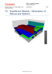
View and edit Flowsheet settings, where the user can change or restore default
settings of the flowsheet. Exit saves the settings and leaves this editor, see Fig. 13.
Fig. 13. Flowsheet settings.
2.
3.
Show and hide the flowsheet Name labels, Value labels and Stream tables.
Check and uncheck all Toolbars, which are explained in section 40.3.
Fig. 14. View menu.
Copyright © Outotec Oyj 2014
HSC 8 – Sim Common Tools
December 10, 2014
Research Center, Pori / Petri Kobylin, Lauri
Mäenpää, Matti Hietala, Jussi-Pekka Kentala
14022-ORC-J
10 (26)
Select menu
The Select menu is typically used to edit or move many properties at once. Here the user
can: (see Fig. 15 below)
1.
2.
3.
4.
5.
6.
7.
8.
9.
10.
11.
12.
13.
Select all Units on the flowsheet.
Select all Unit Name Labels on the flowsheet.
Select all Streams on the flowsheet
Select all Stream Name Labels on the flowsheet.
Select all Stream Value Labels on the flowsheet.
Select all Stream Tables on the flowsheet.
Select all (unit and stream) Name Labels on the flowsheet.
Select all (unit and stream) Value Labels on the flowsheet.
Select all Other Text Labels on the flowsheet.
Select All Labels on the flowsheet.
Select all (not including stream tables) Tables on the flowsheet.
Select all Other Drawing Objects on the flowsheet.
Select All Items on the flowsheet.
Fig. 15. Select menu.
Copyright © Outotec Oyj 2014
HSC 8 – Sim Common Tools
December 10, 2014
Research Center, Pori / Petri Kobylin, Lauri
Mäenpää, Matti Hietala, Jussi-Pekka Kentala
14022-ORC-J
11 (26)
Tools menu
The Tools menu includes many advanced options that may be needed in flowsheet
simulation. The user needs detailed instructions on how to use those tools. Some tools are
explained here and others in different Chapters, see the list below. The Tools menu
includes (see Fig. 17):
1.
Process information
Fig. 16. The user can add Process Information to this sheet.
2.
3.
4.
5.
6.
7.
8.
LCA Evaluation (see Chapter 49)
Mass Balancing (see Chapters 51 and 52)
Reports (see section 40.2.1)
Select Unit Models (see section 40.2.2)
Scenario Editor (see section 40.2.3)
Show the process tree (see section 40.2.4)
Errors in flowsheet (shows possible errors in the flowsheet)
Fig. 17. Tools menu options.
Copyright © Outotec Oyj 2014
HSC 8 – Sim Common Tools
December 10, 2014
Research Center, Pori / Petri Kobylin, Lauri
Mäenpää, Matti Hietala, Jussi-Pekka Kentala
40.2.1.
14022-ORC-J
12 (26)
Reports
A summary of flowsheet results can be saved and printed here. There are two pages in this
report sheet: one for units and one for streams. This report uses Hydro_example3.Sim8.
Fig. 18. Stream balance sheet of the report file.
Fig. 19. Unit balance sheet of the report file.
Copyright © Outotec Oyj 2014
HSC 8 – Sim Common Tools
December 10, 2014
Research Center, Pori / Petri Kobylin, Lauri
Mäenpää, Matti Hietala, Jussi-Pekka Kentala
40.2.2.
14022-ORC-J
13 (26)
Select Unit Models
The user can choose different models for the units. The Select Unit Models window can be
opened from the Tools menu or by right-clicking if the cursor is on top of one of the units,
see Fig. 20. On the left side of the window is the list of units on the flowsheet. In the middle
part the user can select a unit model from the Reactions, Distribution, Particle and Others
sheet (and in the HSC8 update also ‘Import own unit models’). Double-click the unit to
select it and then click OK. Most of the units are dll type but there are still some Excel
Wizards available for the Reactions units. If Excel Wizards are chosen, the user needs to
check the stream names. Information about the units can be found on the right side of the
selector window. Empty Reactions or Distributions units are the same as R and D unit Icons
on the main flowsheet DrawBar, see Fig. 1.
In the HSC8 update that comes later, there will be instructions on how users can make their
own dll units (Chapter 50). User-made units can be imported using the import sheet.
Fig. 20. Select Unit Models window.
Copyright © Outotec Oyj 2014
HSC 8 – Sim Common Tools
December 10, 2014
Research Center, Pori / Petri Kobylin, Lauri
Mäenpää, Matti Hietala, Jussi-Pekka Kentala
40.2.3.
14022-ORC-J
14 (26)
Scenario Editor
The Scenario Editor lets you run your process model with different operating parameters
and see how they affect process variables. The calculated results can then be collected in
the charts.
To use the Scenario Editor, first select the processing parameter that you want to regulate
and copy its cell reference from the appropriate cell. Next, open the Scenario Editor and
paste the cell reference in the first SET/GET column (Fig. 21). Then you can add a name
and measurement unit for this variable, but most importantly you should specify whether the
variable will be a regulated (SET) or a calculated variable (GET) (Fig. 22).
Fig. 21. Add variables to the Scenario Editor by pasting the cell reference of the variable cell.
Copyright © Outotec Oyj 2014
HSC 8 – Sim Common Tools
December 10, 2014
Research Center, Pori / Petri Kobylin, Lauri
Mäenpää, Matti Hietala, Jussi-Pekka Kentala
14022-ORC-J
15 (26)
Fig. 22. Specify the SET/GET value for the variable.
After adding enough variables, specify the parameter values for the SET columns, add
some charts, and finally run the scenario (Fig. 23).
Fig. 23. After specifying the variables, enter the SET variable values, add charts, and run the
scenario.
Copyright © Outotec Oyj 2014
HSC 8 – Sim Common Tools
December 10, 2014
Research Center, Pori / Petri Kobylin, Lauri
Mäenpää, Matti Hietala, Jussi-Pekka Kentala
14022-ORC-J
16 (26)
The calculation results will then be presented in the spreadsheet as well as in the charts
(Fig. 24).
Fig. 24. Results of the scenario.
Copyright © Outotec Oyj 2014
HSC 8 – Sim Common Tools
December 10, 2014
Research Center, Pori / Petri Kobylin, Lauri
Mäenpää, Matti Hietala, Jussi-Pekka Kentala
40.2.4.
14022-ORC-J
17 (26)
Show Process Tree
With this option the user can see the flowsheet information and connections of the process
streams with colors. If a stream is not connected to the unit, it will not be visible in this
process tree.
Fig. 25. Show process tree.
Copyright © Outotec Oyj 2014
HSC 8 – Sim Common Tools
December 10, 2014
Research Center, Pori / Petri Kobylin, Lauri
Mäenpää, Matti Hietala, Jussi-Pekka Kentala
14022-ORC-J
18 (26)
Drawing Tools menu
The user can edit the flowsheet using Drawing Tools by aligning, sizing, rotating, grouping,
and drawing, see Fig. 26.
One handy way of editing the flowsheet is Edit Pages and Layers where you can set layers
and properties which are visible or invisible on your flowsheet, see Fig. 27.
The user can find more details about Drawing Tools in section 40.3.
Fig. 26. Drawing tools.
Fig. 27. Edit Pages and Layers window.
Copyright © Outotec Oyj 2014
HSC 8 – Sim Common Tools
December 10, 2014
Research Center, Pori / Petri Kobylin, Lauri
Mäenpää, Matti Hietala, Jussi-Pekka Kentala
14022-ORC-J
19 (26)
Window and Help menus
The Window menu shows the user the name of the flowsheet, see Fig. 28.
The Help menu shows a list of software developers and technical advisors and a link to the
Sim manual, see Fig. 29 and Fig. 30.
Fig. 28. Window menu.
Fig. 29. Help menu.
Fig. 30. About HSC8 Sim.
Copyright © Outotec Oyj 2014
HSC 8 – Sim Common Tools
December 10, 2014
Research Center, Pori / Petri Kobylin, Lauri
Mäenpää, Matti Hietala, Jussi-Pekka Kentala
40.3.
14022-ORC-J
20 (26)
Toolbars
In the View Toolbars menu, the user can check and uncheck toolbars. It is also possible to
reset docking bar positions back to their default places. Toolbars are divided into two lists:
Docking bars and Drawing toolbars, see Fig. 31.
Fig. 31. List of toolbars.
40.3.1.
Drawing toolbars
The Drawing toolbars are listed and guidance on their usage briefly described in Fig. 32 Fig. 42. Many drawing options can be later edited from docking toolbar Properties after
they have been drawn (section 40.3.2).
Fig. 32. Units and streams. Select or Draw Units or Draw Streams (see also section 40.1).
Fig. 33. Calculations. Simulate and give iteration rounds for calculations.
Copyright © Outotec Oyj 2014
HSC 8 – Sim Common Tools
December 10, 2014
Research Center, Pori / Petri Kobylin, Lauri
Mäenpää, Matti Hietala, Jussi-Pekka Kentala
14022-ORC-J
21 (26)
Fig. 34. Visualization. Select or unselect visualization mode and select the stream property that is
visualized. The user can also change measurement units, open the Stream Table Editor, visualize
stream connections, add a header and copy the flowsheet picture to the clipboard using this toolbar.
Fig. 35. Drawing tool. With this toolbar the user can add shapes like an ellipse, rectangle, rounded
rectangle, pie and chord. It is also possible to add a textbox.
Fig. 36. Height and Width. With this toolbar the user can make the size of the selected units or
streams equal.
Fig. 37. Align. With this toolbar the user can align selected units in many ways, thus making it easier
to draw professional-looking flowsheets.
Fig. 38. Layers. With this toolbar the user can edit pages and layers (Fig. 27) or change the position
of overlapping units.
Fig. 39. Rotate and Flip. With this toolbar the user can rotate or flip units.
Fig. 40. Status bar. With the status bar the user can zoom the flowsheet and check and uncheck the
Persist Tool and Snap to Grid options. The Persist Tool remembers the last used drawing tool so
that the user does not have to select the same tool again separately. The Snap to Grid option aligns
the streams and units according to the grid on the flowsheet, thus making it easier to draw
professional-looking flowsheets.
Fig. 41. FileBar. The user can start a new, open an old, save the current process and save a backup
of the current process using this toolbar.
Fig. 42. TableBar. The user can insert a table using this toolbar (see also section 40.1.4).
Copyright © Outotec Oyj 2014
HSC 8 – Sim Common Tools
December 10, 2014
Research Center, Pori / Petri Kobylin, Lauri
Mäenpää, Matti Hietala, Jussi-Pekka Kentala
40.3.2.
14022-ORC-J
22 (26)
Docking bars
Fig. 43. Log viewer. This docking bar shows the user possible warnings and errors found during the
simulation.
Fig. 44. Process Tree. In this docking bar the user sees the flowsheet as a process tree.
Copyright © Outotec Oyj 2014
HSC 8 – Sim Common Tools
December 10, 2014
Research Center, Pori / Petri Kobylin, Lauri
Mäenpää, Matti Hietala, Jussi-Pekka Kentala
14022-ORC-J
Fig. 45. Properties - Unit Process and Drawings.
Fig. 46. Properties - Stream Process and Drawings.
Copyright © Outotec Oyj 2014
23 (26)
HSC 8 – Sim Common Tools
December 10, 2014
Research Center, Pori / Petri Kobylin, Lauri
Mäenpää, Matti Hietala, Jussi-Pekka Kentala
14022-ORC-J
24 (26)
Fig. 47. Process Errors.
Fig. 48. Unit Icons (Unit List Panel). With this docking bar the user can add Unit pictures to the
flowsheet. The unit pictures are of generic type (see section 40.2.2). The user can switch the view,
browse picture location, search by name, or change unit directory (top bar) or zoom icons (bottom
bar).
Fig. 49. Info and Links. The user can add for example instructions on how to use the flowsheet here.
Copyright © Outotec Oyj 2014
HSC 8 – Sim Common Tools
December 10, 2014
Research Center, Pori / Petri Kobylin, Lauri
Mäenpää, Matti Hietala, Jussi-Pekka Kentala
14022-ORC-J
25 (26)
Fig. 50. Stream Content Viewer. In this docking bar the user can see a tabulated summary of the
stream properties.
Fig. 51. Stream Visualization Settings. In this docking bar the user can change the settings of the
Sankey diagram (thickness of the stream shows where most of the material goes).
Copyright © Outotec Oyj 2014
HSC 8 – Sim Common Tools
December 10, 2014
Research Center, Pori / Petri Kobylin, Lauri
Mäenpää, Matti Hietala, Jussi-Pekka Kentala
40.4.
14022-ORC-J
26 (26)
Importing HSC Sim 7 models (HSC Sim 6 models are not supported)
In HSC Sim 8 there is a built-in support for importing HSC Sim 7 models and then using
them in Sim 8. However, there are some points and limitations that the user should take
into consideration when importing Sim 7 models into Sim 8. If points listed here do not help
please contact the developers.
Major points:
Sim 8 calculations have dramatically stricter error checks than Sim 7. When the user
imports an old model and tries to run it, often the calculation will notify of an error in
the flowsheet. The user can locate the errors using the log viewer and then fix them
manually.
There are some changes in the Sim 8 hydro variable list logic when compared to
Sim 7. If the imported model variable list contains species not found in the database,
the user needs to go through them case by case in the Sim 8 variable list editor. The
user can add entries to the database, use a different database entry, or delete the
species from the variable list to fix this (see Chapter 43, section 43.2.1).
Sim 7 solvent extraction hydro Excel Wizards are no longer supported in Sim 8. If
the imported model contains them in Sim 8, the user will not be able to run the
model successfully.
There is a completely new DLL unit operation system in Sim 8, which has been
implemented for some Mineral Process unit operation models. Sim 8 has partial
support for using old Sim 7 minpro Excel Wizard models and the user should be
able to run calculations for the imported Sim 7 minpro Excel Wizards. However, the
user cannot currently edit or make the Excel Wizards for the old minpro models. If
users want to edit their old mineral process models, they should replace the old
minpro Excel Wizards with the new DLL models.
Minor points:
Sim 8 uses different Stream Tables than Sim 7. Because of this, users cannot edit
Sim 7 Stream Tables in Sim 8 but they can make new ones using Sim 8 tools.
The visibility of the connected streams is forced on for input and output streams in
Sim 8. If there are any such streams hidden in the imported Sim 7 model, they will
appear in Sim 8.
A few drawing objects like a Bézier curve are not supported in the first version of
Sim 8.
In some rare cases, Sim 8 does not recognize Sim 7 stream connections correctly.
Information about this will be given in the import log. Afterwards the user should
manually confirm the notified stream connections.
In Sim 7, the user had the possibility to encrypt some units. This function is no
longer supported in Sim 8, which means those units will not be loaded during the
import.
External workbook references work differently in Sim 7 and Sim 8. When you import
a Sim 7 model, all external references are changed and will include “REF” at the
beginning of the reference.
Sim 7 used automatically safe division for all division operations in the workbook.
This meant that, for example, 0/0 did not give an error as the answer. Sim 8 adds
the “safediv” function to division operations.
Sim 8 will change the sheet names of the workbook if the sheet contains illegal
characters like “/”.
Copyright © Outotec Oyj 2014
HSC 8 - Sim Distribution Units
November 25, 2014
Research Center, Pori / Lauri Mäenpää, Antti
Roine
14022-ORC-J
1 (12)
41. Sim Distribution (Pyro) Units
The Distribution unit, also known as the Pyro unit, is a basic unit type in which output
species are formed based on the element distribution. This distribution can be defined
manually, and regulated further with controls. The Distribution unit also offers Mixer and
Equilibrium wizards which allow you to produce the output species without defining the
element distribution.
Copyright © Outotec Oyj 2014
HSC 8 - Sim Distribution Units
November 25, 2014
Research Center, Pori / Lauri Mäenpää, Antti
Roine
41.1.
14022-ORC-J
2 (12)
Steps to Successful Sim Distribution Simulation
It is important to add the necessary information before simulation can be started. It is good
to follow this list while making your Sim Distribution models. Steps 2 to 5 are explained in
more detail here.
1.
2.
3.
4.
5.
6.
7.
41.2.
Draw units and streams
Specify input streams
Specify output streams
Specify distribution
Set controls
Save process
Run process
Specify Input Streams
The unit editor for a distribution unit is shown in Fig. 1. Information about the input streams
is specified on the Input sheet. The data of the streams are presented in rows. For the input
streams, you should specify: the total amount of the stream, the measurement unit for the
total amount, temperature, pressure, species, and composition.
Fig. 1. Distribution unit editor.
Copyright © Outotec Oyj 2014
HSC 8 - Sim Distribution Units
November 25, 2014
Research Center, Pori / Lauri Mäenpää, Antti
Roine
41.2.1.
14022-ORC-J
3 (12)
Total Amount, Temperature and Pressure
The total amount of the input stream is specified in the cell next to the stream name (Fig.
2). The measurement unit for the total amount is set next to the total amount value (Fig. 3).
Please note that the selected measurement unit (t/h, kg/h or Nm3/h) will determine the
composition percentage unit (wt % or vol %).
Fig. 2. Total amount of the stream.
Fig. 3. Measurement unit for the total amount.
The temperature and pressure values can be changed from the cells below the total
amount (Fig. 4).
Fig. 4. Temperature and pressure of the stream.
41.2.2.
Species and Composition
The species of the stream are entered in the white cells below the stream's header rows
(Fig. 5).
Fig. 5. Enter species in the streams.
Once all the species have been entered, then the composition can be specified (Fig. 6). Please pay
attention to the composition percentage units.
Copyright © Outotec Oyj 2014
HSC 8 - Sim Distribution Units
November 25, 2014
Research Center, Pori / Lauri Mäenpää, Antti
Roine
14022-ORC-J
4 (12)
Fig. 6. Composition of a stream.
The above steps need to be repeated for all of the input streams which act as raw material
inputs. If an input stream is not a raw material input but a stream from another unit, then the
properties of this stream cannot be edited on the Input sheet of the destination unit. The
energy feeds (or heat losses) can be entered in the streams using the buttons in the lefthand panel (Fig. 7).
Fig. 7. Inserting an energy feed into a stream.
Copyright © Outotec Oyj 2014
HSC 8 - Sim Distribution Units
November 25, 2014
Research Center, Pori / Lauri Mäenpää, Antti
Roine
41.3.
14022-ORC-J
5 (12)
Specify Output Streams
On the Output sheet, the same steps need to be carried out as those done for the Input
sheet, with the exception of specifying the total amounts and the stream compositions (Fig.
8). The amounts and compositions of the output streams are usually specified on the Dist
sheet, but there are also wizards which can be used to specify these properties. Specifying
the distribution is introduced in section 41.4.
Fig. 8. The user needs to specify: the measurement unit for the amounts, temperature, pressure,
and the species for the output streams.
Copyright © Outotec Oyj 2014
HSC 8 - Sim Distribution Units
November 25, 2014
Research Center, Pori / Lauri Mäenpää, Antti
Roine
41.4.
14022-ORC-J
6 (12)
Specify Distribution
The distribution of the elements from the Input sheet to the Output sheets can be done by
using the Dist sheet or by using the Mixer or Equilibrium wizards.
41.4.1.
Dist Sheet
You can create the distribution manually by filling the Dist sheet, which is synchronized with
the Output sheet. The elements need to be distributed to the streams and the species
within those streams. Therefore, the common approach is to first distribute the elements to
streams, and then to species. For instance, in this example, the elements H, N and O need
to be distributed to two streams. The first stream contains gaseous species (N2(g), O2(g)
and H2O(g)) and the second stream contains pure water (H2O) (Fig. 9).
Fig. 9. Dist sheet.
The types of distribution of elements to streams can be Fixed, Rest, and Float:
Fixed - Constant or function value is used.
Rest - All the rest of the element goes into this stream.
Float - Automatically fixed by other elements.
In this example, all the nitrogen is distributed to the first stream and hydrogen and oxygen
are distributed to both streams. For instance, it can be initially set that 60% of hydrogen is
distributed to the first stream and the rest to the second stream. For oxygen, the distribution
type in the second stream will be set as "Float" and "Rest" in the first stream (Fig. 10).
Copyright © Outotec Oyj 2014
HSC 8 - Sim Distribution Units
November 25, 2014
Research Center, Pori / Lauri Mäenpää, Antti
Roine
14022-ORC-J
7 (12)
Fig. 10. Distribution of elements to streams.
Next, the elements in the streams will be distributed to the available species. All the species
within a stream need to be assigned an element in column Y and a "Fixed" or "Rest" value
in column X, which shows how the element amount is distributed to the species.
In this example, H2O can be assigned with all of the hydrogen distributed to the second
stream. For the stream with gaseous species, all of the nitrogen will be distributed to the
N2(g), all of the hydrogen to the H2O(g), and the remaining oxygen to the O2(g) (Fig. 11).
Fig. 11. Elements distributed to species.
NB! When all the elements have been correctly distributed to the species, the element
balance, on row 4, should show zero values for all the elements. This ensures that all the
atoms are conserved in the distribution unit.
Copyright © Outotec Oyj 2014
HSC 8 - Sim Distribution Units
November 25, 2014
Research Center, Pori / Lauri Mäenpää, Antti
Roine
41.4.2.
14022-ORC-J
8 (12)
Mixer Wizard
If the unit operation does not include any reactions between the species, then the species
can be distributed directly to the output streams with the Mixer wizard. For the Mixer wizard,
you do not need to specify the species for the Output sheet, but you need to specify the
measurement unit for the amounts. Please also note that the Mixer wizard requires that the
same measurement unit is used for all the streams (both input and output).
The Mixer wizard option is found on the left-hand panel (Fig. 12). Distribution in the wizard
is specified using percentages for each of the output streams (Fig. 13).
Fig. 12. Using the Mixer wizard.
Fig. 13. Distributing species with the Mixer wizard.
Copyright © Outotec Oyj 2014
HSC 8 - Sim Distribution Units
November 25, 2014
Research Center, Pori / Lauri Mäenpää, Antti
Roine
41.4.3.
14022-ORC-J
9 (12)
Equilibrium Wizard
The composition of output streams can also be calculated with the Equilibrium wizard. This
allows you to distribute the elements from the input sheet to species in the Output streams,
based on their chemical stability at the specified output temperature.
The Equilibrium wizard option is found on the left-hand panel (Fig. 14) and the equilibrium
results are presented on the Gibbs sheet, which is linked to the Output sheet. You need to
specify the Input sheet as well as the Output sheet for the wizard. The streams on the
Output sheet are assumed to be separate phases in the equilibrium calculations (Fig. 15).
Phases can be set either as a mixture or as pure phases.
Fig. 14. Using the Equilibrium wizard.
Fig. 15. Distributing elements with the Equilibrium wizard.
Copyright © Outotec Oyj 2014
HSC 8 - Sim Distribution Units
November 25, 2014
Research Center, Pori / Lauri Mäenpää, Antti
Roine
41.5.
14022-ORC-J
10 (12)
Set Controls
Fig. 16. Controls sheet with two controls.
The HSC Sim Controls sheet makes it possible to create controls that regulate the target
parameter cell value using another variable cell value, Fig. 16. In principle, Sim Control
works exactly like a real process control. For example, in a real process unit you can give a
set point to the process unit temperature and regulate the temperature by changing the fuel
oil feed.
To create a control on the Controls sheet, you have to set at minimum the Set Point, the
Target cell reference, Variable cell reference, the limits for the variable, and the tolerance.
You can type this information on the Controls sheet using the following procedure:
1. Type the name and the measurement unit into Controls sheet cells D9 to D10
(optional).
2. Type the Target set value (Set Point) into cell D11.
3. Locate the Target cell in your active unit and right-click "Copy cell reference".
4. Go to Controls sheet cell D12 and right-click "Paste cell reference".
5. Give the tolerance of the calculation in cell D13. When the difference of Set Point and
Measured value is smaller than the Tolerance, the control is in balance and will not be
calculated further.
6. Type the name and the unit of measure in cells D16 and D17 (optional).
7. Locate the Variable cell in your active unit and select "Copy cell reference".
8. Go to Controls sheet cell D18 and right-click "Paste cell reference".
9. Type Limit Min and Max in cells D19 and D20, a narrow numerical range speeds up
the calculations.
The default Tolerance is +/-. A small tolerance increases the calculation time and a large
tolerance increases errors. Some 2% of the target value may be a good compromise. The
control will not be taken into account if the value is within the tolerance.
Copyright © Outotec Oyj 2014
HSC 8 - Sim Distribution Units
November 25, 2014
Research Center, Pori / Lauri Mäenpää, Antti
Roine
14022-ORC-J
11 (12)
Sim Controls have exactly the same limitations as real process controls, for example:
- If the target cell does not depend on the variable cell value, the iterations will fail.
- If an external variable cell is used, there may be a long delay before the effect on the
target value becomes visible. In these cases a lot of iteration rounds might be needed
to reach the Set Point. This increases the calculation time.
Table 1. Information on the Controls sheet.
Row
8
9
10
11
12
13
15
16
17
18
19
20
21
23
24
25
26
27
1
Name
Y Target Name
Process Unit
Measurement Unit
Set Point
Measured
Tolerance +/X Variable Name
Process Unit
Measurement Unit
Value
X Min Limit
X Max Limit
X Max Step
Control Method
Active
Iterations max limit
Iterations min limit
Operation
Description
Name of Y (optional)
Unit name (optional)
Name of the unit of measure (optional)
Set point of Y (obligatory)
Y cell reference (obligatory)
Y tolerance (obligatory)
Name of X (optional)
Unit name (optional)
Name of the unit of measure (optional)
X cell reference (obligatory)
Min limit of the X range (obligatory)
Max limit of the X range (obligatory)
Maximum X Step (optional, default = empty)
Iteration method (optional, default = Auto1)
Set control ON/OFF (optional, default = empty = ON)
Max number of iterations (optional, default = 10)
Min number of iterations (optional, default = empty)
Control calculation operation (optional, default = Light2)
Auto (Solves the control with information on rows 24 - 27), Auto Smart (Same as Auto except changes X Max Step and
Iterations max limit when needed), PID (not in use, will be added to the HSC8 version).
2
Light (Solves the control with modified tangent method, fast), Robust (Solves the control with modified Newton method,
slow), Simple direct (Increases X value when Measured value is too small. The step used can be specified in X max step.),
Simple reverse (Decreases X value when Measured value is too small. The step used can be specified in X max step.).
41.5.1.
Internal and External Controls
1. Internal control in which the target and variable cells exist in the same process unit
(FAST).
2. External control in which the target and variable cells exist in different process units
(SLOW).
Calculation of an internal control is fast because only one unit is calculated. Usually you can
create a large number of internal controls in a process without a dramatic drop in
calculation speed, because they do not increase the number of calculation rounds of the
process.
Calculation of an external control might take more time because material must be
recirculated within the whole process several times to reach a stable target value. Usually
only a few external controls can be used in one process without a considerable decrease
in the calculation speed, because external controls might multiply the calculation rounds of
the process.
Copyright © Outotec Oyj 2014
HSC 8 - Sim Distribution Units
November 25, 2014
Research Center, Pori / Lauri Mäenpää, Antti
Roine
41.5.2.
14022-ORC-J
12 (12)
Advice When Using Controls
- It is recommended to moderate large changes of the variable with the use of X Max
Step, when using external controls with slow responses.
- The RecoveryX add-in function cannot be used in the Target cell, because it is
recalculated only after all the calculation rounds have been completed.
- The large number of thermochemical add-in functions (StreamH, StreamS, etc.) may
reduce the calculation speed if the argument value changes in each control iteration
round, because the data search from the H, S, and Cp database takes time. Use
these add-in functions only when necessary.
Copyright © Outotec Oyj 2014
HSC 8 - Sim Distribution
November 25, 2014
Research Center, Pori / Lauri Mäenpää, Antti
Roine
14022-ORC-J
1 (22)
42. Sim Distribution Example
Magnetite Oxidation Example
Pelletized magnetite (Fe3O4) ore can be oxidized to hematite (Fe2O3) in a shaft furnace.
The typical magnetite content of the ore is approx. 95%. Oxidation is usually done by
feeding air into the shaft furnace. Some excess oxygen is needed to complete the reaction;
the free oxygen in process gas is usually approx. 5%. About 1% of the iron does not react.
Coal is used as a fuel to keep the product temperature at 700 °C.
This kind of unit process can be controlled by air and coal feeds. The ore feed can be fixed
to approx. 200 t/h. Now, please create a process model of the shaft furnace with oxygen
and coal controls.
Walkthrough steps:
1. Draw the flowsheet
2. Draw the streams on the flowsheet
3. Rename the units and streams
4. Save the process
5. Specify the raw material streams
6. Specify the output streams
7. Create a model
a. Distribution to output streams
b. Distribution to species within streams
8. Create the controls
9. Run the process model
Copyright © Outotec Oyj 2014
HSC 8 - Sim Distribution
November 25, 2014
Research Center, Pori / Lauri Mäenpää, Antti
Roine
42.1.
14022-ORC-J
2 (22)
Step 1. Draw the flowsheet
Fig. 1. Draw unit (distribution) on the flowsheet.
First, draw the flowsheet for the process. Usually it is easiest to start with the units of the
process (Fig. 1). You can draw a generic unit and select its model from the Unit Model
Editor, or simply draw a distribution unit by using the red unit icon.
Copyright © Outotec Oyj 2014
HSC 8 - Sim Distribution
November 25, 2014
Research Center, Pori / Lauri Mäenpää, Antti
Roine
42.2.
14022-ORC-J
3 (22)
Step 2. Draw the Streams on the Flowsheet
Fig. 2. Draw streams on the flowsheet.
The second step is to draw streams (Fig. 2), which must be done using the Stream tool on
the left toolbar. The shapes and colors at the end points of the streams indicate their
connections. You can also check the Source and Destination units for each stream from the
Process tab. If a stream is not connected from either end, then this value is shown as a
question mark (?) for the missing Source or Destination value.
Process raw material streams do not have specified Sources, whereas the Destination units
are missing for the process output streams. Intermediate streams should have both Source
and Destination values specified.
Copyright © Outotec Oyj 2014
HSC 8 - Sim Distribution
November 25, 2014
Research Center, Pori / Lauri Mäenpää, Antti
Roine
42.3.
14022-ORC-J
4 (22)
Step 3. Rename the Units and Streams
Fig. 3. Renaming units and streams makes flowsheet easier to read.
You can relocate the unit and stream name labels by dragging them with the mouse. Select
the unit or stream and rename it using the NameID property. This property is used to
identify unit and stream objects. Please use short and illustrative names.
The Drawings tab lets you change the label text formatting. Formatting options can be
applied to the labels one by one, or you can select multiple labels and change the
formatting for all of them. The Select menu at the top bar offers options to select all certain
types of labels from the flowsheet.
Copyright © Outotec Oyj 2014
HSC 8 - Sim Distribution
November 25, 2014
Research Center, Pori / Lauri Mäenpää, Antti
Roine
42.4.
14022-ORC-J
5 (22)
Step 4. Save the Process
Fig. 4. A process has to have a folder of its own.
It is better to save the process too often rather than too seldom, because a saved process
allows you to recover the earlier design stage in case of user or computer errors.
It is necessary to create a separate file folder for each process using the Create New Folder
tool, see Fig. 4. The process name is also the most logical name for the file folder. In this
case the folder name is Magnetite Oxidation and the process name is Magnetite Oxidation.
A process can consist of several files and all of these files will be saved into this same
folder.
Copyright © Outotec Oyj 2014
HSC 8 - Sim Distribution
November 25, 2014
Research Center, Pori / Lauri Mäenpää, Antti
Roine
42.5.
14022-ORC-J
6 (22)
Step 5. Specify the Raw Material Streams
Fig. 5. Raw materials on the Input sheet.
You can open Unit Editor by double-clicking the unit icon on the flowsheet. The raw material
streams can be found on the Input sheet. At the beginning these streams are empty.
Species can be typed into streams manually.
Fig. 6. Specify stream species, compositions, raw material amounts and measure units.
You need to specify the raw material stream species as well as their compositions and
temperatures. It is also important to specify the measure units for the streams. Valid
selections are:
- t/h
- kg/h
- Nm3/h (only for gases)
Please note that the stream composition is given in wt-%, if mass units are used, and in vol%, if normal cubic meters are used. If the feed amount is not yet available then it is good to
specify an initial value such as 1 t/h, especially if this raw material will be used within some
control.
Copyright © Outotec Oyj 2014
HSC 8 - Sim Distribution
November 25, 2014
Research Center, Pori / Lauri Mäenpää, Antti
Roine
42.6.
14022-ORC-J
7 (22)
Step 6. Specify the Output Streams
Fig. 7. Output streams are specified on the Output sheet.
You need to specify the species, temperatures, and the measure units of the output
streams. Please note that the output stream amounts and species distributions cannot be
edited manually, as they will be calculated later.
The Output and Dist sheet streams have been synchronized with each other. This means
that when you type species on the Output sheet they will also appear on the Dist sheet.
Copyright © Outotec Oyj 2014
HSC 8 - Sim Distribution
November 25, 2014
Research Center, Pori / Lauri Mäenpää, Antti
Roine
42.7.
14022-ORC-J
8 (22)
Step 7. Create A Model
Fig. 8. Element distributions need to be specified on the Dist sheet.
The Sim Distribution mode automatically calculates the total input amounts for the input
streams and converts these into elements. The user must specify on the Dist sheet how
these elements will be distributed:
a) into output streams
b) into species within one stream
The Popup list tool can be used in the specification procedure. This tool is automatically
opened when you click a cell where the operation is possible. The options are:
- Fixed
The distribution is fixed with a constant %-value or an Excel-type formula.
Only a constant value cell may be used as a variable on the Controls sheet!
- Rest
When all the specifications have been made for a certain element, then the remaining
fraction of the element must go to one species and one phase.
- Float
This option means that the current cell has been automatically specified by the other
elements like metals. It is usually wise to specify oxygen, sulfur, etc. as floating elements.
Copyright © Outotec Oyj 2014
HSC 8 - Sim Distribution
November 25, 2014
Research Center, Pori / Lauri Mäenpää, Antti
Roine
42.7.1.
14022-ORC-J
9 (22)
Step 7.a - Distribution to Output Streams
Fig. 9. Distribution to output streams.
When distributing the elements to output streams, it might be helpful to hide the species
rows with the "Dist Sheet Rows" button in the left-hand panel (Fig. 9).
An easy way to start is to fix the elements which are present only in one stream. In this
example, this applies to nitrogen (N), iron (Fe), and silicon (Si). Nitrogen is present only in
the "Process Gas" stream, whereas iron and silicon are only found in the "Hematite Pellets"
stream. To distribute these elements, set their status to Fixed in the correct streams and
give their wt-% value as 100 (Fig. 10). Note that you can also use the Rest status for the
elements that are found only in one stream.
Fig. 10. Fixing elements (N, Fe, and Si) in the output streams.
Copyright © Outotec Oyj 2014
HSC 8 - Sim Distribution
November 25, 2014
Research Center, Pori / Lauri Mäenpää, Antti
Roine
14022-ORC-J
10 (22)
For elements that are present in several streams, distribution can be done e.g. by fixing a
value for one stream and letting the remaining amount go to the other. For example, you
can define that 0.1 wt-% of carbon (C) goes into the "Hematite Pellets" stream and the rest
will be distributed to the "Process Gas" stream. To do this, set the status of carbon to Fixed
in the "Hematite Pellets" stream and give the wt-% value as 0.1, then set the status of
carbon in the "Process Gas" stream as Rest (Fig. 11).
Fig. 11. Fixed fraction of carbon in the pellets stream and rest in the gas stream.
Finally, oxygen needs to be distributed to the output streams. In the "Hematite Pellets"
stream, oxygen is present in iron oxides and silica. By letting the iron and silicon content of
the pellet stream determine the amount of oxygen, the status can be set as Float. The rest
of the oxygen will be distributed to the "Process Gas" stream by setting the status as Rest
(Fig. 12).
Fig. 12. Distribution of oxygen to output streams.
Please note that after the elemental distribution to the output streams is finished, the wt-%
values in row 7 should all be 100.
Copyright © Outotec Oyj 2014
HSC 8 - Sim Distribution
November 25, 2014
Research Center, Pori / Lauri Mäenpää, Antti
Roine
42.7.2.
14022-ORC-J
11 (22)
Step 7.b - Distribution to Species within Streams
Fig. 13. Distribution of elements to species.
All the species in the streams need to be assigned with an element in column Y and a
status in column X. These parameters together are used to distribute the elements to
species. Species that contain only a single element have their element assigned
automatically.
In the "Hematite Pellets" stream, it is easiest to start with carbon (C) and silica (SiO2). For
carbon atoms, there is only one species (C), so this species can be assigned to contain
100% of the stream's carbon content. Similarly, you can fix the silica amount by assigning
the species to the element Si, and setting the species to contain 100% of the stream's
silicon content (Fig. 14).
Fig. 14. Carbon and silicon distribution in the pellets stream.
Copyright © Outotec Oyj 2014
HSC 8 - Sim Distribution
November 25, 2014
Research Center, Pori / Lauri Mäenpää, Antti
Roine
14022-ORC-J
12 (22)
Iron is distributed between magnetite (Fe3O4) and hematite (Fe2O3). In this example, it is
assumed that almost all of the magnetite is oxidized. This can be simulated by fixing 1% of
stream's iron content to Fe3O4 and distributing the rest to Fe2O3 (Fig. 15).
Fig. 15. Iron distribution to the pellets stream.
Next, the elements can be distributed to the "Process Gas" stream. Again, an easy way to
start is to distribute the nitrogen (N) atoms to the only species (N2(g)) which contains
nitrogen (Fig. 16).
Fig. 16. Nitrogen distribution in the gas stream.
For the carbon-containing species (CO(g) and CO2(g)), it can be assumed that enough
oxygen is provided for all of the carbon in the gas stream to be oxidized into carbon dioxide.
Thus, carbon (C) can be assigned to both species and the CO(g) will be fixed at 0.00, and
for CO2(g) the status can be set as Rest (Fig. 17).
Copyright © Outotec Oyj 2014
HSC 8 - Sim Distribution
November 25, 2014
Research Center, Pori / Lauri Mäenpää, Antti
Roine
14022-ORC-J
13 (22)
Fig. 17. Carbon distribution in the gas stream.
The final thing to do is to distribute all excess oxygen atoms (O) to oxygen gas (O2(g)). This
can be done by setting the status to Rest (Fig. 18).
Fig. 18. Oxygen distribution in the gas stream.
Now the distribution of elements in the output streams is ready. It is important to notice that
for a correctly filled Dist sheet, the Balance value for all of the elements is equal to zero
(Fig. 19). This indicates that all the atoms are conserved, and thus the elemental balance is
maintained.
Fig. 19. Zero values indicate that all the atoms are conserved.
Copyright © Outotec Oyj 2014
HSC 8 - Sim Distribution
November 25, 2014
Research Center, Pori / Lauri Mäenpää, Antti
Roine
42.8.
14022-ORC-J
14 (22)
Step 8. Create the Controls
Controls are often used to regulate distribution values, output stream compositions and
heat balances. For each control we have to specify:
1) A target cell and a Set Point value for this cell
2) A variable cell used to regulate the target cell
The variable cell must have some effect on the target cell parameter. If this is not true, then
the control will not work. The situation is exactly the same when you control real processes
and plants.
In this example two controls are used: one to regulate the O2 content in the "Process Gas"
stream, and another to ensure that the heat balance is maintained.
First, add two controls to the sheet by clicking the Add New Control button in the left-hand
panel, and type the name of the first control (Fig. 20).
Fig. 20. Controls can be added to the sheet with the Add New Control button.
Next, set the cell reference for the target parameter. For this control, the correct cell can be
found on the Output sheet, cell D13 (Output!D13). To set this cell reference, you can go to
the Output sheet, right-click the correct cell and select Copy cell reference (Fig. 21).
Copyright © Outotec Oyj 2014
HSC 8 - Sim Distribution
November 25, 2014
Research Center, Pori / Lauri Mäenpää, Antti
Roine
14022-ORC-J
Fig. 21. Copy the cell reference of O2 % in the gas stream.
Then set this cell reference as the control by selecting Paste cell reference for the
Measured value of the O2 % control, cell D12 (Fig. 22).
Fig. 22. Set cell reference for the target parameter.
Copyright © Outotec Oyj 2014
15 (22)
HSC 8 - Sim Distribution
November 25, 2014
Research Center, Pori / Lauri Mäenpää, Antti
Roine
14022-ORC-J
16 (22)
For this target parameter you must assign the Set Point value, which will be the goal that
the control tries to reach. In this example, the Set Point value will be 5.00 vol-%. It is also
recommended to add the process unit and measurement unit to the control (Fig. 23).
Having the units in the controls helps to keep track of their operation.
Fig. 23. Assign Set Point value for the control.
Next, set the variable cell reference that will regulate the target parameter. In this example,
you can use the total input of the "Air" stream. To set this cell reference, go to the Input
sheet and copy the correct cell reference (Input!D22) (Fig. 24), and paste the cell reference
on the Controls sheet to the Value cell (Controls!D18). Also fill in the process and
measurement unit information for the variable parameter (Fig. 25).
Copyright © Outotec Oyj 2014
HSC 8 - Sim Distribution
November 25, 2014
Research Center, Pori / Lauri Mäenpää, Antti
Roine
14022-ORC-J
17 (22)
Fig. 24. Copy cell reference of the air feed.
Fig. 25. Set cell reference for the variable parameter.
Finally, it is recommended to adjust the minimum and maximum limits for the variable
parameter and to set a tolerance value for the target parameter (Fig. 26). After that the
O2% control is ready.
Copyright © Outotec Oyj 2014
HSC 8 - Sim Distribution
November 25, 2014
Research Center, Pori / Lauri Mäenpää, Antti
Roine
14022-ORC-J
18 (22)
Fig. 26. Variable limits and target tolerance.
The Heat Balance control can be made by following the same steps. First, copy the cell
reference for the Total H balance (Dist!J4) (Fig. 27).
Fig. 27. Copy cell reference of the total enthalpy balance.
Then paste this cell reference to the Measured cell of the Heat Balance control and assign
0.00 as the Set Point (Fig. 28).
Copyright © Outotec Oyj 2014
HSC 8 - Sim Distribution
November 25, 2014
Research Center, Pori / Lauri Mäenpää, Antti
Roine
14022-ORC-J
19 (22)
Fig. 28. Set the Total H balance as the target parameter.
The variable to regulate the heat balance can be set as the amount of coal fed into the
furnace. Copy the cell reference of the "Coal" stream's total amount (Input!D15) (Fig. 29)
and paste it to the Value cell of the Heat Balance control (Fig. 30).
Fig. 29. Copy cell reference of the coal feed.
Copyright © Outotec Oyj 2014
HSC 8 - Sim Distribution
November 25, 2014
Research Center, Pori / Lauri Mäenpää, Antti
Roine
14022-ORC-J
20 (22)
Fig. 30. Set Coal feed as the variable.
To complete the process controls, add a tolerance value for the heat balance and adjust the
minimum and maximum limits for the coal feed (Fig. 31).
Fig. 31. Completed controls.
Copyright © Outotec Oyj 2014
HSC 8 - Sim Distribution
November 25, 2014
Research Center, Pori / Lauri Mäenpää, Antti
Roine
42.9.
14022-ORC-J
21 (22)
Step 9. Run the Process Model
The process model is now ready and you can start the simulation by pressing the Simulate
button at the top bar (Fig. 32). Next to the Simulate button you can set the number of
iteration rounds. Processes with recycling streams and controls may require several
iteration rounds in order to reach steady state.
Fig. 32. Simulate the process.
Results of the simulation can be shown on the flowsheet by selecting the Stream
Visualization Mode (Fig. 33). The selected property in the adjacent dropdown menu is
shown in each of the stream value labels (Fig. 34).
Fig. 33. Stream Visualization.
Visualization can be used with the simulation to study, whether the process reaches steady
state. After a few simulation rounds, the value labels should obtain values which no longer
change when further simulation rounds are run. It is also recommended to check the
controls (Fig. 35). They are OK if the Set Point has been reached within the tolerance.
Copyright © Outotec Oyj 2014
HSC 8 - Sim Distribution
November 25, 2014
Research Center, Pori / Lauri Mäenpää, Antti
Roine
14022-ORC-J
22 (22)
Fig. 34. Element balances and behavior can be seen when element amounts are selected in the
visualization. In this screenshot, the diagram shows the behavior of oxygen in the process.
Fig. 35. Controls after simulation.
Copyright © Outotec Oyj 2014
HSC 8 – Sim Reactions Unit
November 25, 2014
Research Center, Pori / Petri Kobylin, Tuukka
Kotiranta
14022-ORC-J
1 (15)
43. Sim Reactions (Hydro) Unit
The Reactions unit calculates chemical reactions based on unit operations in solid, liquid,
and gas systems. This unit was originally made for hydrometallurgical process calculations,
but can be used for almost any process, especially those that can be modeled with
chemical reactions.
Copyright © Outotec Oyj 2014
HSC 8 – Sim Reactions Unit
November 25, 2014
Research Center, Pori / Petri Kobylin, Tuukka
Kotiranta
43.1.
14022-ORC-J
2 (15)
Steps to Successful Sim Reactions Simulation
It is important to add the necessary information before the simulation can be started. It is
good to follow this list while making your Sim Reactions models. Steps 3 to 9 are explained
in more detail below.
1.
2.
3.
4.
5.
6.
7.
8.
9.
43.2.
Draw units and streams, see Chapter 40 (section 40.1.)
Save Process (see step 8)
Create variable list
Add reaction equations
Specify distributions
Set controls
Specify raw material amounts
Save Process and Save Backup
Run process
Creating a Variable List
A variable list editor is shown in Fig. 1. The user should at least add some species to
phases in this editor. In this simple (cooler) example, only H2O has been added to the water
phase (row 13) and just the amount has been checked (cell E12), which automatically
creates row 17. Default system variables are also shown in rows 3-9 and default phases in
rows 10, 12, and 15.
Fig. 1. Variable List Editor where user specifies the variables needed in the simulation.
43.2.1.
Filling Variable List Manually
Specify the Species
First you need to specify the species you are using in your calculation. The species can be
any combination of elements (like Fe, Ag, O, etc.), solid species (CaCO3, Na2S, CuS, etc.),
Copyright © Outotec Oyj 2014
HSC 8 – Sim Reactions Unit
November 25, 2014
Research Center, Pori / Petri Kobylin, Tuukka
Kotiranta
14022-ORC-J
3 (15)
gases (CO2(g), O2(g), N2(g), etc.), or liquids (H2SO4(a), CuSO4(a), etc. or Cu(+2a), SO4(2a), H(+a), etc.).
Special case: species that are not found in HSC database
If the compound is not found from the HSC database. To use the compound you need to
add it to the own database.
Here are instructions what you need to take into account when you add the compound:
The compound needs to have a chemical formula. Molecular weight is calculated from the
formula. For mixtures use formula that gives average molecular weight and if you do not
know the exact formula use formula that has correct molecular weight.
For example organic compound with average molecular weight of 350 g/mol can be put to
the database as: C29(MPEG350).
Note that the last character in brackets defines the phase so it cannot be any of the
following characters: a, g, l, s, + or -.
You can add properties to the compound manually, for example enthalpy (kJ/mol), entropy
(J/(mol*K)), heat capacity (J/(mol*K)) and density (kg/l). For heat capacity you can fit data
for different temperature ranges.
If you know the chemical formula for the compound the enthalpy, entropy and heat capacity
values can be estimated with H, S and Cp estimates module.
Example
Organic compound
In copper solvent extraction you have unloaded reagent, loaded reagent and diluent that
are not found from the HSC database. You know the density and molecular weight of the
compounds. This is one way how you add the compounds to the database.
Type the compound name to the variable list editor. It will open the database editor
automatically and copy the compound name to editor if compound is not found from the
database.
Type the data for the compound (name and density in units kg/l):
C42H2(unloaded reagent), 0.96
C42Cu(loaded reagent), 1.00
C14(diluent), 0.79
If you know enthalpy, entropy or heat capacity values you can add them for the compounds.
After adding compounds to the database and the densities you can use these organic
compounds in your model. The density for the organic phase is calculated automatically
from the fed data. The compounds can be used in chemical reactions just like other
compounds.
Copyright © Outotec Oyj 2014
HSC 8 – Sim Reactions Unit
November 25, 2014
Research Center, Pori / Petri Kobylin, Tuukka
Kotiranta
14022-ORC-J
4 (15)
Divide the Species into Phases
Divide the species into meaningful phases, because only this will enable you to calculate
phase properties like densities and compositions, Fig. 1. Species can be typed manually or
they can be imported from the database.
A) Type species formulae manually into <enter species> cells.
B) Go to cell <enter species>, click database button, select species and click Import items
button in Database Browser.
Specify the Variables
Phase
Measurement units of different phases
Gas (Nm3/h, t/h, kg/h)
Water, Particles, Organic, Solid (t/h, kg/h)
Default phases are "Gas Phase", "Water Phase", and "Pure Phase". The user can change
phase names and add new phases as well using the Modify button or delete phases using
Remove.
Concentrate (Concentration)
Measurement units of different phases
Gas (wt %, vol % or ppm)
Water (wt %, g/l or ppm)
Pure (wt % or ppm)
Mass Fraction
To calculate mass fractions of the Water phase, the user has to give
A compound which is found in Density Database (Al2(SO4)3…ZnSO4)
A compound (aqueous ion) which is found in the variable list (Al(+3a)…Zn(+2a))
Other
Specify Name (e.g. Solid concentration)
Specify Unit (e.g. g/l)
User Formula
Specify Name (e.g. Solid concentration)
Specify Unit (e.g. g/l)
Insert an Excel-type formula in Column D (e.g. =D13/D7/1000. HSC functions like
Molecular weight, MW(“H2O”), can also be used in the formulae)
43.2.2.
Importing Ready-Made Variable List
A custom-made variable list allows you to utilize the HSC Sim module in many different
types of simulation applications, such as mineralogical, chemical, hydrometallurgical,
pyrometallurgical, economic, biological, etc. Only your imagination sets the limits! The
custom-made variable list gives a lot of flexibility but the drawback is that the users have to
know what they are doing.
This is also the main reason why the specification of the variable list is one of the most
important tasks in the new model development stage. It is easy to add/delete/modify the
Copyright © Outotec Oyj 2014
HSC 8 – Sim Reactions Unit
November 25, 2014
Research Center, Pori / Petri Kobylin, Tuukka
Kotiranta
14022-ORC-J
5 (15)
variable list later on, but it may still be best to try to specify a complete variable list right at
the beginning or at least before you start to create the calculation models.
If you have a ready-made variable list available you can use the Import button in the
Variable list editor and choose the *.xls or *.xlsx file that includes your variable list. Some
example files can be found in the HSC Chemistry installation folder …\Flowsheet_Hydro.
43.2.3.
Activating Variable List
After filling the variable list manually or importing it, the next thing is to click Activate.
43.2.4.
Summary of Columns
The meaning of the Input, Output, and Dist sheet columns can be summarized as follows:
Column A - Type: Specifies the row type:
-
T
Pr
A
H
V
Ex
Cp
P
D
C
F
O
U
Temperature
Pressure
Amount
Enthalpy
Volume
Exergy
Heat Capacity
Phase
Species
Density (mass fractions also need to be specified for water phase species)
Concentration (concentrate)
Mass Fraction (base species must be specified)
Other
User formula
The number section in the row type parameter refers to the phase number. For example:
A2 = Amount of phase 2, H3 = enthalpy of phase 3, etc.
Column B - Variable: Specifies the variable name.
Column C - Unit: Specifies the measurement unit. Use the same measurement units within
all the process unit models.
Column D - Formula: Specifies the Excel-type cell formula which will automatically be
added into model Input and Output sheets in Column D and in all the stream columns. HSC
AddIn functions can also be used, e.g. MW("H2O").
The HSC AddIn function =Units ("C";"MJ") will check whether the temperature and energy
units are as specified in the formula. The user may change the measurement units only in
the variable list editor.
Columns E - Streams: Each stream has a column of its own.
Copyright © Outotec Oyj 2014
HSC 8 – Sim Reactions Unit
November 25, 2014
Research Center, Pori / Petri Kobylin, Tuukka
Kotiranta
43.3.
14022-ORC-J
6 (15)
Adding Reaction Equations to Create Calculation Model
In the reactions unit, the mathematical connection (model) between the Input and Output
streams is created using Chemical Reactions Wizard. This model transforms the raw
materials into products by using chemical reactions given by the user, see Fig. 3.
Fig. 2. In Chemical Reactions Wizard the user specifies reaction equations and their progress.
The first step is to enter the reactions that happen in the process unit in the Chemical
Reactions Wizard, Fig. 2. The species used in the reactions must exist in the variable list.
The first species of each reaction is assumed to be the "raw material" which is consumed in
this reaction according to the progress %. For example, FeS is the raw material in reaction
1. You must keep in mind that more than 100% of the raw materials cannot be consumed.
The sum of Progress % cannot be more than 100% for the same raw material, although it
may be less than 100%. The other species in the reaction equations will automatically be
taken into account when a model is created based on the reaction stoichiometry. However,
it is still recommended to check whether there are negative amounts on the Model sheet
and remove them, for example, by decreasing the Progress %.
The second step is to test the balances by pressing the Balance button. This gives an OK in
the Balance column, showing that everything is acceptable. The balance test will also give
enthalpy H and equilibrium constant K for the reaction at 25 °C if all the species are found
in the active HSC databases. Negative H values mean that heat is released in the reaction,
whereas positive values mean that more heat is needed. Large K values (>1) mean that the
reaction tends to go to the right and small values (<1) mean that the reaction tends to go to
the left in the equilibrium state.
The third step is to Activate the reaction equations. After that the reactions can be seen on
the model sheet. This sheet contains a list of the reactions with progress percentages. The
user may change the Progress % cells (H7 and H11) manually or by using a control, see
Fig. 3. NB! The species name is red if it is not found in the variable list. This will lead to
material balance errors since the missing species will not be copied to the output sheet.
Copyright © Outotec Oyj 2014
HSC 8 – Sim Reactions Unit
November 25, 2014
Research Center, Pori / Petri Kobylin, Tuukka
Kotiranta
14022-ORC-J
7 (15)
Fig. 3. Model sheet shows user-defined chemical reactions.
43.3.1.
Unit Model Editor - Excel Wizards
Ready-made Excel wizards for some units like Filter and Thickener were used in HSC7.
These wizards are also available in HSC8; however, they will no longer be supported in the
future so we recommend users not to use them any more. New dll units can be used for this
purpose.
Unit model editor is activated from the Tools menu in the main flowsheet window (or right
mouse click over any unit). In the editor, the user can choose a unit, double-click the wizard
and click OK. The user then specifies the streams and after that the model is ready to be
used, see also Chapter 40 (section 40.2.2).
Copyright © Outotec Oyj 2014
HSC 8 – Sim Reactions Unit
November 25, 2014
Research Center, Pori / Petri Kobylin, Tuukka
Kotiranta
43.4.
14022-ORC-J
8 (15)
Distributions
The Dist sheet is filled because the user must divide the products into the output streams. If
there is only one output stream then 100% of the products enter this stream. The example
in Fig. 4 shows a distribution where all the gas species enter the Offgas stream (type 100 in
cell F14) and all the water and pure species go to the solution phase (type 100 in cells E18
and E24).
Fig. 4. Dist sheet is usually filled with given distribution percentages.
Copyright © Outotec Oyj 2014
HSC 8 – Sim Reactions Unit
November 25, 2014
Research Center, Pori / Petri Kobylin, Tuukka
Kotiranta
43.5.
14022-ORC-J
9 (15)
Creating Controls
Controls can be added, removed and seen using quick links on the left column, see Fig. 5.
Fig. 5. The calculation model “Controls sheet” with one control.
The HSC Sim Controls sheet makes it possible to create controls that regulate the target
parameter cell value using another variable cell value, see Fig. 5. In principle, Sim Control
works exactly like a real process control. For example, in a real process unit you can assign
a set point to the process unit temperature and regulate the temperature by changing the
fuel oil feed.
To create a control on the Controls sheet, you have to set at least the set point, the Target
cell reference, the Variable cell reference, the limits for the variable, and the tolerance. You
can type this information on the Controls sheet using the following procedure:
1. Type the name and the unit of measure in Control sheet cells C4 to C6 (optional).
2. Type Target set value in cell C7.
3. Locate the Target cell from your active unit and right mouse click "Copy cell
reference".
Copyright © Outotec Oyj 2014
HSC 8 – Sim Reactions Unit
November 25, 2014
Research Center, Pori / Petri Kobylin, Tuukka
Kotiranta
14022-ORC-J
10 (15)
4. Go to Control sheet cell C8 and right mouse click "Paste cell reference".
5. Give the tolerance of the calculation in cell C9. When the difference between the Set
Point and the Measured value is smaller than the Tolerance, the control is in balance
and will not be calculated further.
6. Type the name and the unit of measure in cells C12 and C13 (optional).
7. Locate the Variable cell from your active unit and select "Copy cell reference".
8. Go to Control sheet cell C14 and right mouse click "Paste cell reference".
9. Type Limit Min and Max in cells C15 and C16; a narrow numerical range speeds up
the calculations.
The default Tolerance is +/-. A small tolerance increases the calculation time and a large
tolerance increases errors. Some 2% of the target value may be a good compromise. The
control will not be taken into account if the value is within the tolerance.
Sim Controls have exactly the same limitations as real process controls, for example:
- If the target cell does not depend on the variable cell value, the iterations will fail.
- If an external variable cell is used, there may be a long delay before the effect on the
target value becomes visible. In these cases a lot of iteration rounds might be needed
to reach the set point. This increases the calculation time.
Table 1. Information on the Control sheet.
Row
4
5
6
7
8
9
11
12
13
14
15
16
17
19
20
21
22
23
1
Name
Y Target Name
Process Unit
Measurement Unit
Set Point
Measured
Tolerance +/X Variable Name
Process Unit
Measurement Unit
Value
X Min Limit
X Max Limit
X Max Step
Control Method
Active
Iterations max limit
Iterations min limit
Operation
Description
Name of Y (optional)
Unit name (optional)
Name of the unit of measure (optional)
Set point of Y (obligatory)
Y cell reference (obligatory)
Y tolerance (obligatory)
Name of X (optional)
Unit name (optional)
Name of the unit of measure (optional)
X cell reference (obligatory)
Min limit of the X range (obligatory)
Max limit of the X range (obligatory)
Maximum X Step (optional, default = empty)
Iteration method (optional, default = Auto1)
Set control ON/OFF (optional, default = empty = ON)
Max number of iterations (optional, default = 10)
Min number of iterations (optional, default = empty)
Control calculation operation (optional, default = Light2)
Auto (Solves the control with information on rows 20 - 23), Auto Smart (Same as Auto except changes X Max Step and
Iterations max limit when needed), PID (not in use, will be added to HSC8 version).
2
Light (Solves the control with modified tangent method, fast), Robust (Solves the control with modified Newton method,
slow), Simple direct (Increases X value when Measured value is too small. The step used can be specified in X max step.),
Simple reverse (Decreases X value when Measured value is too small. The step used can be specified in X max step.).
Copyright © Outotec Oyj 2014
HSC 8 – Sim Reactions Unit
November 25, 2014
Research Center, Pori / Petri Kobylin, Tuukka
Kotiranta
43.5.1.
14022-ORC-J
11 (15)
Internal and External Controls
1. Internal control in which the target and variable cells exist in the same process unit
(FAST).
2. External control in which the target and variable cells exist in different process units
(SLOW).
Calculation of an internal control is fast because only one unit is calculated. Usually you can
create a large number of internal controls in a process without a dramatic drop in
calculation speed because they do not increase the number of calculation rounds of the
process.
Calculation of an external control might take more time because material must be
recirculated within the whole process several times to reach a stable target value. Usually
only a few external controls can be used in one process without a considerable decrease
in the calculation speed because external controls might multiply the calculation rounds of
the process.
Sometimes it is easier to set controls using additional sheets, where some calculations may
be done. You can insert new sheet using left column quick link Insert Custom Sheet or by
using menu Insert…Sheet.
43.5.2.
Advices When Using Controls
- It is recommended to moderate large changes of the variable with the use of X Max
Step when using external controls with slow responses.
- If you want to keep some concentration lower than a set point (8 g/l), change the
bleed stream amount (valve 0 - 100%). Please use an external control since the bleed
amount will not change the concentration unless the whole process is calculated. This
is possible when the bleed and concentration cells are in different units.
- The RecoveryX add-in function cannot be used in the Target cell, because it is
recalculated only after all the calculation rounds have been completed.
- The large number of thermochemical add-in functions (StreamH, StreamS, etc.) may
reduce the calculation speed if the argument value changes in each control iteration
round, because the data search from the H, S, and Cp database takes time. Use
these add-in functions only when needed.
Copyright © Outotec Oyj 2014
HSC 8 – Sim Reactions Unit
November 25, 2014
Research Center, Pori / Petri Kobylin, Tuukka
Kotiranta
43.6.
14022-ORC-J
12 (15)
Adding Raw Materials
In both input and output sheets if the cells are white it means that the user can edit them.
43.6.1.
Input Sheet
In the input sheet, temperature row 7, pressure row 8, and the raw material amounts are
given. In the example in Fig. 6, the amount of H2O and FeS is known and the O2(g) and
N2(g) amounts are calculated using equations, whereas the H2SO4 amount is calculated
using the control. The user can give an initial guess of the sulfuric acid value in cell F20 or it
can also be empty before the simulation is started.
If the flowsheet contains more than one unit and the units are connected, intermediate
stream properties cannot be edited since these values are calculated, see Fig. 7.
Fig. 6. Input sheet, raw material amounts.
Copyright © Outotec Oyj 2014
HSC 8 – Sim Reactions Unit
November 25, 2014
Research Center, Pori / Petri Kobylin, Tuukka
Kotiranta
14022-ORC-J
Fig. 7. Input streams of the second unit cannot be edited.
Copyright © Outotec Oyj 2014
13 (15)
HSC 8 – Sim Reactions Unit
November 25, 2014
Research Center, Pori / Petri Kobylin, Tuukka
Kotiranta
43.6.2.
14022-ORC-J
14 (15)
Output Sheet
In the output sheet, temperature row 7 and pressure row 8 are given, see Fig. 8. Values in
the output sheet are calculated according to the settings in the Dist and Model sheets.
Fig. 8. Output sheet, temperature and pressure of the streams can be changed.
Copyright © Outotec Oyj 2014
HSC 8 – Sim Reactions Unit
November 25, 2014
Research Center, Pori / Petri Kobylin, Tuukka
Kotiranta
43.7.
14022-ORC-J
15 (15)
Save and Run simulation and visualize results
It is good to Save Process and Backup often. It is good habit to save process after each
step. Remember to save at least before starting the simulation, see Fig. 9 and Fig. 10.
There are many ways to visualize the simulation results, see Fig. 11 and Chapter 40
(section 40.3.).
Fig. 9. Save Process and Save Backups icons.
Fig. 10. Run simulation and give iteration rounds to calculations.
Fig. 11. Visualize results and change units, add stream tables, visualize stream connections, add
header or copy flowsheet to clipboard.
Copyright © Outotec Oyj 2014
HSC 8 - Sim Reactions Example
November 25, 2014
Research Center, Pori / Petri Kobylin, Tuukka
Kotiranta
14022-ORC-J
1 (15)
44. Sim Reactions Example
44.1.
General
This example contains instructions on how to create a simple leaching reactor model where
10 t/h of FeS is leached with acid (H2SO4) and air at 70 °C. The water feed is 50 t/h and the
FeS leaching efficiency is 90 %, oxygen efficiency is 50 %, and the acid concentration in
the product is 1 g/l.
The reactor is cooled with cooling coils. The cooling water input temperature is 25 °C and
output temperature 60 °C.
You should keep in mind that streams are put into the input and output sheets in the same
order as you have drawn them. This means that when you make a new model the streams
might be in a different column than explained here.
The example files can be found from the HSC Chemistry installation folder
…Flowsheet_Hydro\Hydro_example3\Hydro_example3.Sim8. This example describes the
creation of the flowsheet in detail with references to the Sim Flowsheet manual.
Fig. 1. Sim Reactions Example flowsheet.
Copyright © Outotec Oyj 2014
HSC 8 - Sim Reactions Example
November 25, 2014
Research Center, Pori / Petri Kobylin, Tuukka
Kotiranta
44.2.
14022-ORC-J
Steps to Successful Sim Reactions Simulation
1.
2.
3.
4.
5.
6.
7.
8.
9.
Draw units and streams
Save process and save backup
Create variable list
Add reaction equations
Specify distributions
Set controls
Specify raw material amounts
Save process
Run process
Copyright © Outotec Oyj 2014
2 (15)
HSC 8 - Sim Reactions Example
November 25, 2014
Research Center, Pori / Petri Kobylin, Tuukka
Kotiranta
44.2.1.
44.2.2.
14022-ORC-J
3 (15)
Drawing a Flowsheet, See Chapter 40 (section 40.1.)
-
Draw Reactions units (blue).
-
Draw input and output streams. Left mouse click to start and make corners and
double-click to end the stream. For editing the stream afterwards, see section 40.1.2.
-
Name the units and streams, see Fig. 1 and Chapter 40 (section 40.1.3.).
-
Check that the source and destination for the streams are correct.
Setting the Variable List, See Chapter 43 (section 43.2.)
A) Import Ready-Made Variable List
In this example two variable lists can be used. You can add the lists to the model by
double-clicking the unit and clicking Variable List Editor (or in Excel editor, Tools menu and
Variable List Editor) and by pressing Import…\Flowsheet_Hydro\Hydro_example3\. For the
Leaching unit we choose Leaching.xlsx and for the Cooler unit Cooler.xlsx, see Fig. 2
and Fig. 3. It is also possible to use Leaching.xlsx list for the Cooler unit but not vice versa.
B) Fill Variable List Manually
You can also fill in the variable lists manually, see Fig. 2 and Fig. 3, or Chapter 43. Use
Nm3/h unit for the Gas Phase. You need to give the mass fractions of the water phase
otherwise density cannot be calculated (see rows 33-34 in Fig. 2). Since H2SO4
concentration in g/l is not in the list, you need to create a User Formula (U) in the Variable
List Editor.
-
Choose User formula and give it a name (H2SO4 concentration) and measure unit
(g/l).
-
Make the formula in column D, see Fig. 2. In the example above, the formula in cell
D35 is D19/MW(“H”)/2*MW(“H2SO4”)/D30*1000, which means that mass of H2SO4 is
calculated from the amount of H(+a) ions in moles (see equation in Fig. 4) divided by
the water phase volume. The result is multiplied by 1000 to obtain the unit grams of
H2SO4 per liter of solution.
-
The User formula is copied automatically to all the Input and Output streams of each
unit when Activate is clicked. NB! The equation is changed in the Variable List Editor
to “=SAFEDIV(SAFEDIV(D19;MW("H"))/2*MW("H2SO4");D30)*1000” (with equation
SAFEDIV HSC8 Sim sets 0/0 = 0).
When modifying the variable list, remember that columns A to D are automatically
synchronized, which means that any changes are automatically copied to all the streams.
Copyright © Outotec Oyj 2014
HSC 8 - Sim Reactions Example
November 25, 2014
Research Center, Pori / Petri Kobylin, Tuukka
Kotiranta
14022-ORC-J
Fig. 2. Variable list of the Leaching unit.
Fig. 3. Variable list of the Cooler unit.
Copyright © Outotec Oyj 2014
4 (15)
HSC 8 - Sim Reactions Example
November 25, 2014
Research Center, Pori / Petri Kobylin, Tuukka
Kotiranta
44.2.3.
14022-ORC-J
5 (15)
Add Reaction Equations to the Unit (Chapter 43 section 43.3.)
The following leaching reaction equations:
FeS + H(+a) + O2(g) = Fe(+2a) + S + H2O (90 % efficiency)
H2SO4 = H(+a) + SO4(-2a) (100 % efficiency)
can be added with the Chemical Reactions Wizard. In the Leaching unit, open the Excel
editor "Chemical Reactions Wizard". You have to write the Progress %, Reactants,
Products, and press the Balance button, which checks the coefficients for the reactions, see
Fig. 4.
Fig. 4. Reactions sheet in Chemical Reactions Wizard.
44.2.4.
Specify Distributions
Remember to complete the Dist sheets of the units. In the Leaching unit, 100% of the gas
phase goes to the Offgas stream and 100% of the liquid and solid phase goes to the
Solution stream. Fill in the percentages for both streams, see Fig. 5. In the Cooler unit
there is just one output stream so fill in 100 % to each phase.
Copyright © Outotec Oyj 2014
HSC 8 - Sim Reactions Example
November 25, 2014
Research Center, Pori / Petri Kobylin, Tuukka
Kotiranta
14022-ORC-J
6 (15)
Fig. 5. Dist. sheet of the Leaching unit.
44.2.5.
Setting Controls for the Process, Chapter 43 (section 43.5.)
Controls can be added, removed and seen using quick links on the left column, see Fig. 6.
In the first control sheet, the H2SO4 concentration after leaching is set at 1 g/l of solution by
calculating the input amount of H2SO4, see Fig. 6 and Table 1.
In the second control sheet, the cooling requirements (heat balance) of the highly
exothermic leaching process are set to 0 by calculating the cooling water amount. NB!
Insert an extra sheet in the Cooler unit, see Fig. 7 to Fig. 10 and Table 2.
Copyright © Outotec Oyj 2014
HSC 8 - Sim Reactions Example
November 25, 2014
Research Center, Pori / Petri Kobylin, Tuukka
Kotiranta
14022-ORC-J
7 (15)
Fig. 6. Controls sheet of the Leaching unit.
Table 1. Data for controlling the H2SO4 concentration after leaching.
Row name (Cell)
Filled value or formula
Set point (C7)
Measured (C8)
Tolerance +/- (C9)
Value (C14)
X Min Limit (C15)
X Max Limit (C16)
1
=Output!E36
0.01
=Input!F20
0
100
Copyright © Outotec Oyj 2014
Notes
Desired H2SO4 concentration, g/l
Measured H2SO4 concentration, g/l
Tolerance for concentration
H2SO4 input to the process, t/h
Minimum amount for H2SO4 input
Maximum amount for H2SO4 input
HSC 8 - Sim Reactions Example
November 25, 2014
Research Center, Pori / Petri Kobylin, Tuukka
Kotiranta
14022-ORC-J
Fig. 7. Insert Custom Sheet and text added to this new sheet (renamed to Extra sheet).
Copyright © Outotec Oyj 2014
8 (15)
HSC 8 - Sim Reactions Example
November 25, 2014
Research Center, Pori / Petri Kobylin, Tuukka
Kotiranta
14022-ORC-J
9 (15)
Fig. 8. Copy cell reference from the Leaching unit and paste cell reference to the extra sheet.
Copyright © Outotec Oyj 2014
HSC 8 - Sim Reactions Example
November 25, 2014
Research Center, Pori / Petri Kobylin, Tuukka
Kotiranta
14022-ORC-J
Fig. 9. Copy cell reference from the Cooler unit and paste cell reference to the extra sheet.
Copyright © Outotec Oyj 2014
10 (15)
HSC 8 - Sim Reactions Example
November 25, 2014
Research Center, Pori / Petri Kobylin, Tuukka
Kotiranta
14022-ORC-J
11 (15)
Fig. 10. Controls sheet of the Cooler unit.
Table 2. Data for controlling the Heat balance. Measured value is calculated in an additional sheet.
Row name (Cell)
Filled value or formula
Set point (C7)
Measured (C8)
Tolerance +/- (C9)
Value (C14)
X Min Limit (C15)
X Max Limit (C16)
0
=Extra sheet!C4
0.1
=Input!E16
0
1000
Copyright © Outotec Oyj 2014
Notes
Desired Heat balance, kWh
Measured Heat balance, kWh
Tolerance for Heat balance
H2O input to the process, t/h
Minimum amount for H2O input
Maximum amount for H2O input
HSC 8 - Sim Reactions Example
November 25, 2014
Research Center, Pori / Petri Kobylin, Tuukka
Kotiranta
44.2.6.
14022-ORC-J
12 (15)
Setting Feed Streams to the Process
All the feed streams to the process should be set. If the feed to the process is not set, the
stream will be ignored.
Input sheets of both Leaching and Cooler units:
- FeS stream H2O is 50 t/h and FeS is 10 t/h in the FeS stream.
- H2SO4 stream sulfuric acid feed - an initial guess of 1 t/h can be given. Real value
(10.1 t/h) is calculated using the control, see Table 1.
- Air stream consists of 21 vol.% of O2(g) and 79 vol.% of N2(g). Oxygen efficiency is
50 %, which means that 2 times the stoichiometric amount is needed. The formulas
made for oxygen and nitrogen are =ABS(Model!F16)*2 and =G16/21*79,
respectively.
- Cold water stream feed - an initial guess of 10 t/h can be given. Real value (195.8
t/h) is calculated using the control, see Table 2.
Output sheets of both Leaching and Cooler units:
- Temperature of solution and offgas streams should be set to 70 °C, see Fig. 12.
- Temperature of hot water stream should be set to 60 °C.
Fig. 11. Feed stream amounts of the Leaching unit.
Copyright © Outotec Oyj 2014
HSC 8 - Sim Reactions Example
November 25, 2014
Research Center, Pori / Petri Kobylin, Tuukka
Kotiranta
14022-ORC-J
13 (15)
Fig. 12. Output stream temperatures of both Solution and Offgas streams are put at 70 °C.
44.2.7.
Saving the Process, Chapter 40 (sections 40.2. and 40.3.1.)
Processes should always be saved in their own folder. Changing the process name is not
enough since every unit is an Excel file that is saved in the same folder as the flowsheet.
The name of these files is the same as the name of the units. Therefore you also have to
save different scenarios in different folders.
44.2.8.
Running the Simulation and Checking the Results, sections 40.3.1 and 40.3.2
When you have finished the model you can run the simulation. First you have to set the
number of rounds you wish to calculate the process and then press the Simulate button to
start the simulation. You should check if the values change during different runs to find out
if the process is in balance. The value of the selected variable is presented in the value
labels, see Fig. 13. User can add Stream Tables and Header (Chapter 40 sections 40.1.4
and 40.3.1) to visualize the calculation results, see Fig. 14 and Fig. 15.
Copyright © Outotec Oyj 2014
HSC 8 - Sim Reactions Example
November 25, 2014
Research Center, Pori / Petri Kobylin, Tuukka
Kotiranta
14022-ORC-J
Fig. 13. Selecting visualization from the list.
Fig. 14. Stream Table Editor to modify Stream Tables.
Copyright © Outotec Oyj 2014
14 (15)
HSC 8 - Sim Reactions Example
November 25, 2014
Research Center, Pori / Petri Kobylin, Tuukka
Kotiranta
14022-ORC-J
Fig. 15. Stream Tables and Stream Viewer to visualize calculation results.
Copyright © Outotec Oyj 2014
15 (15)
HSC 8 - Sim Minerals Processing
November 20, 2014
Research Center, Pori / Antti Remes, Pertti
Lamberg
14022-ORC-J
45. Sim Minerals Processing
Copyright © Outotec Oyj 2014
1 (35)
HSC 8 - Sim Minerals Processing
November 20, 2014
Research Center, Pori / Antti Remes, Pertti
Lamberg
14022-ORC-J
2 (35)
TOC:
45.1. Introduction .................................................................................................................. 3
45.1.1. Particle-based modeling ....................................................................................... 3
45.1.2. Levels of modeling detail ...................................................................................... 6
45.1.3. Minerals processing flowsheet structure in HSC Sim ........................................... 7
45.1.4. HSC Sim file structure .......................................................................................... 8
45.1.1 Before starting to create a simulation model ............................................................ 8
45.2. Drawing a flowsheet .................................................................................................. 10
45.2.1. Units and unit icons ............................................................................................ 10
45.2.2. Connecting streams ........................................................................................... 10
45.2.3. Checking the flowsheet ...................................................................................... 12
45.3. Stream Setup – Defining the feed composition.......................................................... 13
45.3.1. Solids feed.......................................................................................................... 15
45.3.1.1.Total solids ......................................................................................................... 15
45.3.1.2.Minerals .............................................................................................................. 17
45.3.1.3.Size classes ....................................................................................................... 20
45.3.1.4.Size distribution .................................................................................................. 22
45.3.1.5.Mineral and elemental composition .................................................................... 23
45.3.2. Liquid feed .......................................................................................................... 27
45.3.3. Gas feed ............................................................................................................. 28
45.4. Selecting unit models ................................................................................................ 29
45.5. Run simulation and view the results .......................................................................... 31
45.5.1. Simulate ............................................................................................................. 31
45.5.2. Visualization, tables, graphs, scenarios.............................................................. 31
45.6. Opening an HSC 7 flowsheet in HSC 8 ..................................................................... 34
45.6.1. Conversion from HSC 7 to HSC 8 format ........................................................... 34
45.6.2. Simulating the flowsheet..................................................................................... 34
45.6.3. Modifying feed composition ................................................................................ 34
45.6.4. Editing model parameters and reloading the unit models................................... 35
Copyright © Outotec Oyj 2014
HSC 8 - Sim Minerals Processing
November 20, 2014
Research Center, Pori / Antti Remes, Pertti
Lamberg
45.1.
Introduction
45.1.1.
Particle-based modeling
14022-ORC-J
3 (35)
HSC Sim has a special set-up and approach for processes where minerals are treated. This
approach should be used for processes such as crushing, grinding, flotation, gravity
separation and screening. Mineral-based models treat particles that have at least the
following properties:
size (diameter)
mineral composition in wt.%
In addition, they may have additional parameters like composition by volume%, mineral
composition by surface area%, whiteness, hardness, etc. Each mineral has a certain
chemical composition and specific gravity on the basis of which HSC will calculate these
properties for each particle and also for each stream. Fig. 1 illustrates the solids phase set
up as a particulate material - the approach HSC Sim minerals processing models are based
on.
Fig. 1. Particles of different sizes, consisting of one or more minerals. A colored SEM (Scanning
Electron Microscope) graph (Outotec Research, Pori, Finland).
HSC Sim supports a versatile set-up of the particle-based feed streams, according to the
desired modeling complexity. Each mineral can be a fully liberated material that can be
further be divided into several size classes with particles in them. With a more elaborated
feed set-up, the degree of liberation and association between different minerals in each size
class can be defined. Fig. 2 gives examples of different particle set-ups: liberated (100%
one mineral), binary (two minerals), ternary (three minerals), and complex (four or more
minerals); all of these are possible in HSC Sim.
The feed composition and mineralogy are defined with the HSC Sim Stream Setup tool
complemented by HSC Geo’s extensive mineral database, mineralogical calculation tools,
and MLA (Mineral Liberation Analysis) data file importing and handling possibilities.
Copyright © Outotec Oyj 2014
HSC 8 - Sim Minerals Processing
November 20, 2014
Research Center, Pori / Antti Remes, Pertti
Lamberg
Liberated
14022-ORC-J
Binary
Ternary
4 (35)
Complex
Fig. 2. Different complexities of minerals according to their liberation.
HSC Sim assigns several properties to each particle. A stream consists of a certain ton per
hour amount including that particle type. All the stream properties, such as the element wt%
in it, solid specific gravity, or total solids tons per hour, for example, are always calculated
based on the particle composition of the stream. The particle properties and most common
stream properties are listed below. These stream properties are also at the same time the
initial data for setting up a feed stream for which the particles are automatically generated.
1.
Particle properties
Each particle has its own specific properties that are set when they are created, e.g. in the
feed Stream Setup. They consist of:
A list of minerals, their composition% in a particle and properties including:
Name
Code (name shortening)
Chemical formula
Specific gravity
Chemical composition
Optional: Database reference
Optional: additional properties (user-defined)
Size class information including:
Lower and upper boundary of each class and geometric average
Name label of the size class
Optional: number of particles in a class, in case of MLA file imported particles
Optional: particle floatability parameters for flotation kinetics based separation
Optional: particle type, indicating its mineral association group, typically with MLA file
imported particles.
2.
Stream properties (feed)
Streams consist of numerous properties and calculated values derived from their particle
composition. The feed stream particles are generated by HSC Sim based on the following
data:
Total solids input of the stream (t/h)
Weight percentage of each size class (totaling 100%)
Weight percentage of each mineral in each size class (totaling 100%) and in bulk
(calculated)
Chemical composition of fractions and bulk (calculated)
Optional: mineral liberation and association data for each size class. Only if nonliberated particles are to be set up and used in modeling.
Copyright © Outotec Oyj 2014
HSC 8 - Sim Minerals Processing
November 20, 2014
Research Center, Pori / Antti Remes, Pertti
Lamberg
14022-ORC-J
5 (35)
Particle handling in process units:
When a stream is directed to a certain unit in a flowsheet, the particular unit operation of
that unit can treat the particles as follows:
1.
2.
3.
Mix the particles of all the incoming streams and direct the mixture to one or more
outputs.
Break down the particles. This is the only unit operation where (some of) the incoming
particles are destroyed and do not exist in the output. Instead, new particles are
generated so that the total flow rate and mineral balance are held over the unit.
Particles can be separated according to several properties; typically: size, specific
gravity, mineral composition (resulting in the overall flotation kinetics for that particle,
for example), etc…
The above main particle stream phenomena and examples of the unit operations for
these are shown in Fig. 3.
Mixing
Pump sump
Feed box
Mixing tank
…
Breaking Down
Crushing
Grinding
…
Separation, by
Size (e.g.
screening,
hydrocyclones)
Specific Gravity
(e.g. Knelson
concentrator,
hydrocyclones)
Mineral
Composition
(e.g. flotation)
Shape, Color,
etc…
Fig. 3. Examples of unit operations based on the stream particles.
Copyright © Outotec Oyj 2014
HSC 8 - Sim Minerals Processing
November 20, 2014
Research Center, Pori / Antti Remes, Pertti
Lamberg
45.1.2.
14022-ORC-J
6 (35)
Levels of modeling detail
Before starting to build up HSC Sim minerals processing models it is worth considering how much
detail is required, what background data are available, and what type of unit models are available
with what level of detail. Fig. 4 illustrates how the feed material can be defined and thus how the unit
models should be capable of handling stream compositions.
In addition to increasing the level of detail, the number of particles transferred between the
units increases. With large simulation models this might have impact on the simulation
calculation speed (especially in the case of dynamic simulation). Also, quite often
increasing the modeling details means increasing the time needed to build up and
parameterize the simulation model. Fig. 5 lists some of the minerals processing application
areas where different details of modeling are typically applied.
Fig. 4. Levels of modeling detail – required background data.
Copyright © Outotec Oyj 2014
HSC 8 - Sim Minerals Processing
November 20, 2014
Research Center, Pori / Antti Remes, Pertti
Lamberg
14022-ORC-J
7 (35)
Unsized
Sized
No Composition
Mineral / Chemical
Composition
Simple Material t/h
Balance
Crushing
Grinding
Screening
Cyclones
Etc...
Bulk Material:
Flotation
Physical
Separation
Etc...
Sized Particles:
Flotation
Physical
Separation
Comminution
Etc...
MLA Based
Particles Modeling
Fig. 5. Levels of modeling detail – examples of modeling application areas.
45.1.3.
Minerals processing flowsheet structure in HSC Sim
The HSC Sim process flowsheet consists of Units and Streams (Fig. 6). When the
modeling is based on particles, a Stream consists of Solids and Liquid and Gas phases,
although the gas phase is rarely set for a mineral slurry feed stream. The liquid may have
soluble components, but in minerals processing, these species are often ignored, i.e. the
liquid (water) only has density as a parameter. Solids consist of particles which are
composed of minerals. Minerals have properties such as chemical composition. In HSC
Sim all the properties of solids are calculated from particle flow rates, particle compositions,
and mineral properties. For example, copper does not behave independently in the process
but is always bound to a mineral or minerals that occur in particles, which vary in size and
composition.
Fig. 6. Structure of HSC Sim flowsheets for minerals processing.
Copyright © Outotec Oyj 2014
HSC 8 - Sim Minerals Processing
November 20, 2014
Research Center, Pori / Antti Remes, Pertti
Lamberg
45.1.4.
14022-ORC-J
8 (35)
HSC Sim file structure
HSC Sim flowsheet models must always be saved in a separate folder, each of them. This
is because the same file names may exist in the flowsheets, and they must not be mixed
between flowsheets. The folder name can differ from the flowsheet name; they are not
related to each other. The process flowsheet model is in a Sim8 file, and can be opened in
HSC Sim 8 by double-clicking it. Table 1 summarizes the simulation model files located in
the model folder.
NB: A flowsheet model can be copied or sent elsewhere just by sending (zipping) the whole
simulation model folder.
Table 1. HSC Sim files in minerals processing flowsheet models.
Model Component
Flowsheet
Corresponding Files
ProcessName.Sim8
ProcessName.Sim8bin
Unit
Unit_1.xlsx
Unit_2.xlsx
Unit_N.xlsx
Feed_1.HSCStream
Feed_2.HSCStream
Feed_N.HSCStream
Feed Stream
What They Are
Flowsheet layout description
Unit icons, data, etc. related to
the flowsheet
Each unit has a separate file
to store its parameters, state
and settings
Each feed stream has a
separate file to describe the
(particle) feed composition
45.1.1 Before starting to create a simulation model
Before starting to build a process for simulation, you should collect all the relevant data of
the process. According to the data and your aims, you should:
1.
Decide the level of detail you want to have in the drawing and simulation.
Is it necessary to draw all the existing units (e.g. pump sumps), or could the circuit be
simplified without losing any essential information?
It is a good idea to draw a draft of the flowsheet on a piece of paper. That will help
you to position the units correctly.
2.
Decide the level in terms of particles. The possible levels from the lowest (least
information) to the highest are:
a.
b.
c.
d.
Sized model without composition. Typically grinding
circuits are modeled like this. The chemical and mineral
composition of the input (e.g. ROM) is identical to the
output (e.g. flotation feed), and the main interests are in
flow rates and the required energy.
Unsized mineral model. Each mineral is treated
separately but all the size classes are treated together.
Typically a simple flotation model is like this.
Unsized floatability components model. Each mineral is
divided into 2-3 floatability classes, (i.e. fast floating, slow
floating and non-floating) or several (~20) different classes
of floatability distribution (e.g. Klimpel model).
Size-by-mineral model. Each mineral is treated
Copyright © Outotec Oyj 2014
(Typically 5-25
particles)
(Typically 3-8
particles)
(Typically 9150 particles)
(Typically 15-
HSC 8 - Sim Minerals Processing
November 20, 2014
Research Center, Pori / Antti Remes, Pertti
Lamberg
e.
14022-ORC-J
separately by size. This approach enables the simulation
of a full mineral processing circuit including crushing,
grinding, classification, and different kind of separation
techniques like flotation, gravity separation, magnetic
separation, and dewatering.
True particles model. This is the highest level of modeling
where particles treated in the process have been
measured with e.g. MLA and all of them or groups formed
from them are treated in the process.
9 (35)
300 particles)
(Typically 20015 000
particles)
Remember that if you go to a higher-level approach you will need more data and better
models.
3.
List the minerals present in the circuit. Find their chemical composition and specific
gravity. If you do not know, please ask a geologist or mineralogist or look for a
mineralogical report.
4.
Find the chemical composition or mineral composition of the feed streams. If you
have only the chemical composition, do the element to mineral conversion (with HSC
Geo, together with the Sim Stream Setup tool).
5.
Find the flowsheet of the process or if it is a greenfield process, consider possible
alternatives and decide where to start.
6.
Find data for unit models and their parameters. To create models you will need some
experimental data. These are elemental assays from a laboratory test, pilot test, or
survey. If you have data, you can organize the data in HSC using the Mass Balance
module to mass balance and reconcile data (see Chapter 51 Mass Balance). Some of
the simplest models do not have operational parameters like size, length, gap size,
volume, or area, but if you want to use more comprehensive models you should
gather this information as well.
After obtaining the background data, the building of a simulation model comprises the
following main steps:
I.
II.
III.
IV.
V.
VI.
Draw the flowsheet: place the units there, rename them, draw the streams and
rename them
Check that all the streams are connected correctly
If not yet done, next save the flowsheet to a separate folder. Please take backups
every now and then
Define the feed streams: feed rate, select minerals, size classes, size and
mineral/elemental composition, liquid and gas phases
Select and load the unit models and set the parameters and possible controls for
them
Simulate and fine-tune the model. View, visualize and report the results.
These steps are described in more detail in the following sections.
Copyright © Outotec Oyj 2014
HSC 8 - Sim Minerals Processing
November 20, 2014
Research Center, Pori / Antti Remes, Pertti
Lamberg
45.2.
Drawing a flowsheet
45.2.1.
Units and unit icons
14022-ORC-J
10 (35)
The process units can be placed by dragging and dropping them from the Unit Icons panel
on the right; the library includes several ready-made process device icons. Alternatively,
you can just draw a rectangle unit without a figure, by selecting it from the left-side button
bar. The unit figure can also be changed and replaced with your own drawing or
photograph if desired. Selecting and drawing the unit on the flowsheet are shown in Fig. 7.
NB: Unit figures do not contain calculation models, just the graphics to illustrate them on the
flowsheet. The calculation model is selected and loaded separately in a later step.
A)
B)
C)
Fig. 7. Unit model icons can be A) dragged and dropped from the HSC Sim library, B) the library
folder can be changed from the menu; or C) just a generic unit with a rectangle box icon can be
drawn.
45.2.2.
Connecting streams
The streams area drawn on the flowsheet by selecting the stream drawing tool from the bar
on the left (Fig. 8). The streams area is automatically connected to the nearby unit to/from
which they are directed. The streams can be redirected and connected elsewhere on the
flowsheet; HSC Sim will then ask you to confirm whether the stream source/destination
should also be changed (Fig. 9). In addition, the source and destination can be set from the
stream properties panel on the right (Fig. 10).
Copyright © Outotec Oyj 2014
HSC 8 - Sim Minerals Processing
November 20, 2014
Research Center, Pori / Antti Remes, Pertti
Lamberg
14022-ORC-J
11 (35)
Fig. 8. Drawing the streams.
Fig. 9. Setting stream source and destination after redirecting the stream on the flow sheet drawing.
Fig. 10. Stream properties where the Source and Destination can be set.
The streams are renamed by double-clicking the stream name label, or from the stream
properties panel. The value labels – showing the simulated values of the selected variable
in the visualization mode – are inserted automatically. The stream names and value labels
can be modified in terms of font, color, etc. from the properties panel.
Copyright © Outotec Oyj 2014
HSC 8 - Sim Minerals Processing
November 20, 2014
Research Center, Pori / Antti Remes, Pertti
Lamberg
45.2.3.
14022-ORC-J
12 (35)
Checking the flowsheet
When the flowsheet is ready, you should check that all the stream connections are going to
the correct units. The visual notation for the streams is as follows:
Starting point = no shape: stream is an output of a unit
Starting point = white circle: stream is a feed input to the simulation
Ending point = filled arrow: stream goes to an input of a unit
Ending point = white arrow: stream is an output of the simulation that does not go to
any unit
Fig. 11. Example of a flowsheet with units and the streams connecting them.
NB: There is no need to define the stream type as solids/slurry or liquid/water as required in
HSC 7. HSC 8 handles all of the streams in the same manner regardless of the stream
composition.
When the flowsheet is ready and you have checked it is correct, the feed stream(s) can be
defined.
Copyright © Outotec Oyj 2014
HSC 8 - Sim Minerals Processing
November 20, 2014
Research Center, Pori / Antti Remes, Pertti
Lamberg
45.3.
14022-ORC-J
13 (35)
Stream Setup – Defining the feed composition
Feed Streams for HSC Sim minerals processing models are defined by using the Stream
Setup tool. To open Stream Setup:
Right-click a feed stream and select “Define this stream with Stream Setup”
When the stream content is already defined, it can be modified at any time. Open
Stream Setup by double-clicking the stream.
The Stream Setup dialog (Fig. 12) consists of:
Upper bar buttons
Left-side Phases navigation tool
Right-side Properties of selected component
Right-side Graphs of selected component
Middle area for setting up the feed properties
Fig. 12. Stream Setup tool dialog for defining a minerals processing feed stream. The ‘Solids
Composition’ view is shown here.
All the required data is entered in the middle part of the dialog, by navigating the steps on
the left-side Phases navigation panel (Fig. 13). The data can be entered in any order, but
the easiest way is to follow the links from top to bottom, starting from the Solids Total Flow
Rate.
Copyright © Outotec Oyj 2014
HSC 8 - Sim Minerals Processing
November 20, 2014
Research Center, Pori / Antti Remes, Pertti
Lamberg
14022-ORC-J
14 (35)
Fig. 13. Phases navigator to set the stream data step by step.
When the desired stream data have been entered, the stream and its particle content are
saved and updated to the simulation model by clicking Update and Close on the upper bar
(Fig. 14). Alternatively, the changes can be cancelled using the Discard and Close button.
The cell references for the total t/h flow rates of the Solids, Liquid and Gas phases can be
copied by clicking the respective upper bar buttons. The cell reference can then be pasted
and used elsewhere, for example in controls that adjust the flow rates of the feed streams.
Fig. 14. Buttons to apply changes and to copy cell references for the total phase flow rates.
Good to know:
You can always relocate or detach the dialog components as you like
Just drag and drop them to undock & dock elsewhere
You can leave the dialog components floating on the display and resize them freely
The figures have tools that appear when you place the cursor over them: you can
copy, print, clone, etc.
Copyright © Outotec Oyj 2014
HSC 8 - Sim Minerals Processing
November 20, 2014
Research Center, Pori / Antti Remes, Pertti
Lamberg
14022-ORC-J
15 (35)
Fig. 15. Relocate and resize the dialog components by undocking and docking them with the left
mouse button held down.
45.3.1.
Solids feed
Solids feed is based on particles in the HSC Sim minerals processing models (see Fig. 6).
In the simplest form no size classes (bulk flow) and no minerals are defined (thus the
default is bulk ‘Ore’ mineral). To set up the solids feed composition and mineralogy, the
following data need to be defined:
Total Flow Rate
Minerals
Size Classes
Size Distribution
Composition of minerals and elements
45.3.1.1.
Total solids
The total solids are entered in the Amount field; the unit can be changed from the dropdown
menu, and the amount is then automatically recalculated (Fig. 16). NB: The unit in this
selection does not affect the unit shown in the flowsheet simulation. There the flow rates
are shown in t/h.
Copyright © Outotec Oyj 2014
HSC 8 - Sim Minerals Processing
November 20, 2014
Research Center, Pori / Antti Remes, Pertti
Lamberg
14022-ORC-J
16 (35)
Fig. 16. Setting the total solids flow rate and its measure unit.
In addition, the total phase flows can be entered and the measure units changed in the
properties panel on the right (Fig. 17).
Fig. 17. Properties of total phase flows (in the panel on the right).
The total flow rates are visualized in a bar graph, indicating the amounts of solids, liquid
and gas flow rates (Fig. 18).
Fig. 18. Total flow rate graph.
Copyright © Outotec Oyj 2014
HSC 8 - Sim Minerals Processing
November 20, 2014
Research Center, Pori / Antti Remes, Pertti
Lamberg
45.3.1.2.
14022-ORC-J
17 (35)
Minerals
Minerals can be added by selecting them from the HSC Geo mineral database, or a new
mineral can be created from scratch. In both cases the element composition as well as the
specific gravity can be edited freely. The upper bar buttons for setting up the minerals are
shown in Fig. 19.
Fig. 19. Buttons for adding minerals from the database, removing minerals, creating new custom
minerals, and editing their elemental composition.
To open the HSC Geo Select Minerals tool, click Add Mineral
from DB...
You can search for the mineral from the database; once the
selected list is ready, click OK to accept (Fig. 20).
Fig. 20. Selecting minerals from the database.
Once the minerals are added, they will appear on the list, where the name, code, S.G., and
formula can be edited (Fig. 21). The element composition of the minerals is presented in
the lower part of the display, in the Mineral Matrix (Fig. 22).
Fig. 21. List of selected minerals.
The Mineral Matrix allows you to edit the list of included elements; new elements can be
added simply by typing them on the list and/or editing the existing elements. In the same
way, the element wt% in each mineral can be edited.
Copyright © Outotec Oyj 2014
HSC 8 - Sim Minerals Processing
November 20, 2014
Research Center, Pori / Antti Remes, Pertti
Lamberg
14022-ORC-J
18 (35)
Note I: the element wt% in each mineral is typically approximately 100%. However, this is
not necessary; the chemical composition of a mineral can present just the measured
elements for example.
Note II: the editing of the mineral properties (element wt%, S.G., etc.) does not affect them
on the HSC Geo database. The edited minerals properties are only applied in the current
HSC Sim simulation feed stream.
Fig. 22. Mineral matrix for presenting and editing the element compositions of selected minerals.
Alternatively, to edit the Mineral Matrix element list in the lower part of the dialog, elements
can be added, removed, or selected from the periodic table on the Elements button menu,
shown in Fig. 23.
Copyright © Outotec Oyj 2014
HSC 8 - Sim Minerals Processing
November 20, 2014
Research Center, Pori / Antti Remes, Pertti
Lamberg
14022-ORC-J
19 (35)
A)
B)
Fig. 23. Editing of elements, and selecting them from the periodic table.
The selected mineral (Fig. 21) properties are presented on the properties panel on the right
(Fig. 22), and its element composition is presented visually in a pie chart (Fig. 25).
Fig. 24. Mineral properties.
Copyright © Outotec Oyj 2014
HSC 8 - Sim Minerals Processing
November 20, 2014
Research Center, Pori / Antti Remes, Pertti
Lamberg
14022-ORC-J
20 (35)
Fig. 25. Graphical presentation of the elemental composition of a mineral.
45.3.1.3.
Size classes
The sieve size classes can be set up and edited as follows (Fig. 26):
Top Size can be given or left empty; this affects the way the mean size of the
topmost class is calculated
Sieve Size is given and accepted by pressing Enter or the Add Sieve button (Fig.
26); alternatively there is a right mouse button tool for this (Fig. 27)
The selected sieve can be removed by clicking Remove Sieve; or by right-clicking
(Fig. 27)
Create Sieve Series offers a way to create standard sieve series up to the given
Top Size by using (Fig. 28):
ISO 565 Test Sieves
American Standard (ASTM E11)
British Standard (BS 410)
Square root of 2 series (down to > 1 µm)
OR to create a given number of square root 2 series classes (up from 1 µm). In this
case, Top Size is not needed.
Fig. 26. Tool for creating and editing sieve size classes.
Copyright © Outotec Oyj 2014
HSC 8 - Sim Minerals Processing
November 20, 2014
Research Center, Pori / Antti Remes, Pertti
Lamberg
14022-ORC-J
21 (35)
Fig. 27. Size classes view for editing sieves and size class labels.
Fig. 28. Creating of a predefined sieve series.
Both the size class and size distribution properties are summarized on the right-hand panel
(Fig. 29).
The user-editable values in Properties are:
Size Classes:
Select whether the size class labels are generated automatically or edited manually
in the size class list (Fig. 27). These labels can be used in the unit models when you
need to enter model parameters by size
Measurement unit: µm or mm, this affects how the size data is shown in the Stream
Setup tool, but for stream particles, the base unit for size is always the micrometer
Top size, can be given or left empty
Size Distribution:
Type: user-given size assay data or automatically generated distribution based on
Rosin-Rammler or Gaudin-Schuhmann equations
Rosin-Rammler equation parameters: a = 63.2 % passing size, b = distribution
slope.
Gaudin-Schuhmann equation parameters: k = 100% passing size, m = distribution
slope.
The calculated values and information presented in the Properties are (Fig. 29):
Size Classes:
Number of size classes
Indication if the feed is Unsized (bulk) or Sized
Indication if the Top Size is given
Copyright © Outotec Oyj 2014
HSC 8 - Sim Minerals Processing
November 20, 2014
Research Center, Pori / Antti Remes, Pertti
Lamberg
14022-ORC-J
22 (35)
Size Distribution:
Calculated 50% passing size, P50
Calculated 80% passing size, P80
Fig. 29. The size class and size distribution properties.
45.3.1.4.
Size distribution
The size distribution is given as wt% retained values for each size; the last size class is
automatically calculated to total 100% (Fig. 30). Also, the cumulative passing % values are
calculated automatically. Negative values are not allowed, and are indicated by red color,
which must be corrected before proceeding further. If, instead of Assay Data (user-given
values), the Rosin-Rammler or Gaudin-Schuhmann distribution calculation is selected (Fig.
29), the wt% values in Fig. 30 will also be generated automatically.
Fig. 30. Defining the size distribution.
The size distribution (either Rosin-Rammler or Gaudin-Schuhmann) can be calculated in
two ways:
1)
2)
By the equation, based on the two parameters given in Properties (Fig. 29)
By giving the known passing size value (e.g. for P80), the slope parameter is as given
in Properties (Fig. 29), and the second parameter is solved by HSC Sim, by pressing
Enter or clicking Calculate Distribution from the Set Passing Size button menu,
shown in Fig. 31.
Copyright © Outotec Oyj 2014
HSC 8 - Sim Minerals Processing
November 20, 2014
Research Center, Pori / Antti Remes, Pertti
Lamberg
14022-ORC-J
23 (35)
Fig. 31. Automatic calculation of the size distribution to match the given passing size value.
Finally, the cumulative size distribution curve can be seen graphically (Fig. 32). The figure
includes both data points for each given sieve size and the quadratic spline interpolation
curve between them.
Fig. 32. Logarithmic presentation of the cumulative passing size; both the given sieve size data
points and quadratic spline interpolation between them.
45.3.1.5.
Mineral and elemental composition
The mineral compositions and resulting elemental compositions are edited from the tables
shown in Fig. 33. The tables consist of:
Mineral Composition:
= 100: one of the minerals is always calculated as 100 % - the sum of all the other
minerals
Mineral: list of minerals (Codes)
Bulk: bulk composition (cannot be edited when sized data; is then calculated
automatically)
Unit: %
Size fractions: mineral composition of the fractions
Elemental Composition:
Analyzed: indicates if the value is analyzed, thus it will not be updated based on the
minerals. Instead, this is then the initial data for element to mineral conversion
Copyright © Outotec Oyj 2014
HSC 8 - Sim Minerals Processing
November 20, 2014
Research Center, Pori / Antti Remes, Pertti
Lamberg
14022-ORC-J
24 (35)
Element: list of all elements
Bulk: bulk composition (cannot be edited when sized data, is then calculated
automatically), editable for ‘Analyzed’ elements in the case of unsized data
Unit: %
Size fractions: elemental composition of the fractions. These are automatically
calculated based on the minerals, except if the element is marked ‘Analyzed’
be the initial data for element to mineral conversion
Fig. 33. Mineral and elemental composition tables.
When the tables (shown in Fig. 33) are clicked, a graph will show either the mineral or
elemental composition by size, see Fig. 34.
Copyright © Outotec Oyj 2014
will
HSC 8 - Sim Minerals Processing
November 20, 2014
Research Center, Pori / Antti Remes, Pertti
Lamberg
14022-ORC-J
25 (35)
A)
B)
Fig. 34. Bar graphs of A) mineral and B) elemental stream composition for bulk and each size class.
A) Setting mineral composition – elements are calculated
The mineral composition can be simply entered in the upper table by each size class. One
of the minerals is always selected, with = 100, to be calculated as 100% minus all the
other minerals (Fig. 35). The elements are automatically calculated and updated, but only if
they are not marked Analyzed. The analyzed elements are the initial values for element to
mineral conversion – explained in B).
Fig. 35. Entering the mineral wt% and selecting the
= 100 mineral.
Copyright © Outotec Oyj 2014
HSC 8 - Sim Minerals Processing
November 20, 2014
Research Center, Pori / Antti Remes, Pertti
Lamberg
14022-ORC-J
26 (35)
Fig. 36. Analyzed elements, not calculated from minerals, but updated after element to mineral
conversion.
B) Setting element composition – minerals are calculated
Firstly, select the analyzed elements (Fig. 36); these are the initial values
for element to mineral conversion. The conversion is done using HSC
Geo in its Modal Calculations tool. To open HSC Geo for modal
calculation, click the ‘Element to Mineral...’ button. The Modal
Calculations dialog shown in Fig. 37 will open.
The Modal Calculations tool indicates the selected elements in the periodic table and lists
the minerals included in the Stream Setup. The calculation procedure is described in
Chapter 84; in brief the steps are:
Select the mineral(s) for calculation round 1
Select the elements(s) for calculation round 1
Add new calculation round(s) using the (+) ‘Add Round’ button
The last round is practically always marked ‘Sum = 100 %’, thus that mineral is to be
the remaining gangue material
All the calculation rounds are then performed sequentially, with the selected method
when you click ‘Calculate’
When mineral composition calculation results are satisfactory, they are brought to
Stream Setup by clicking ‘Update and Close’
Copyright © Outotec Oyj 2014
HSC 8 - Sim Minerals Processing
November 20, 2014
Research Center, Pori / Antti Remes, Pertti
Lamberg
14022-ORC-J
27 (35)
Fig. 37. HSC Geo Modal Calculations
When the element to mineral calculation with HSC Geo is ready, the results are seen in the
Stream Setup Composition view, Fig. 38. Now, the tooltip of the ‘Analyzed’ values shows
the original assay value, and the difference from it. The value in the corresponding cell
shows the element wt% obtained in the mineral to element back calculation with the HSC
Geo Modal Calculation tool.
Fig. 38. Elements back-calculated from the minerals, after modal calculation in HSC Geo.
45.3.2.
Liquid feed
The total liquid flow rate and its unit can be set in the Total Liquid Flow Rate view, see Fig.
40. Also, the liquid flow rate can be automatically calculated and kept updated, based on
the given solids flow rate and solids percentage (Fig. 39), when the ‘Solids % Target’
button is held down. Otherwise the ‘Sol. %’ text field indicates the calculated solids
percentage based on the given solids and liquid flow rates.
Copyright © Outotec Oyj 2014
HSC 8 - Sim Minerals Processing
November 20, 2014
Research Center, Pori / Antti Remes, Pertti
Lamberg
14022-ORC-J
Fig. 39. Solids % target value for calculating the required liquid t/h
Fig. 40. Total liquid flow rate.
45.3.3.
Gas feed
The total gas phase flow rate is set from the Amount field shown in Fig. 41.
Fig. 41. Total gas total flow rate.
Copyright © Outotec Oyj 2014
28 (35)
HSC 8 - Sim Minerals Processing
November 20, 2014
Research Center, Pori / Antti Remes, Pertti
Lamberg
45.4.
14022-ORC-J
29 (35)
Selecting unit models
The unit models are selected for the unit icons of the flowsheet by using the Select Unit
Models tool Fig. 43, which can be opened by:
HSC Sim menu bar: Tools
Select Unit Models
Right-clicking the unit (Fig. 42)
Double-clicking the unit
Fig. 42. Selecting a unit model for a unit.
The unit models are selected from the model library simply by double-clicking the model
which is then assigned to the selected unit(s), Fig. 43. All the HSC Sim minerals processing
unit models are shown under the Particles tab on the model list. The Select Unit Models
dialog is also described in Chapter 40 (section 40.2.2.).
Fig. 43. Select Unit Models.
Once the models have been applied to the units, the model parameters are next edited and
viewed with the model editor as shown in Fig. 44. The model input and output streams can
be viewed, their connection to the model inputs and outputs can be configured, and controls
for the models can be defined.
Setting up the Controls and Cell References between the units is described in sections
43.5. and 44.2.5.
Copyright © Outotec Oyj 2014
HSC 8 - Sim Minerals Processing
November 20, 2014
Research Center, Pori / Antti Remes, Pertti
Lamberg
14022-ORC-J
30 (35)
Fig. 44. Dialog to enter and view the unit model parameters, stream content, stream connections,
and model controls.
Copyright © Outotec Oyj 2014
HSC 8 - Sim Minerals Processing
November 20, 2014
Research Center, Pori / Antti Remes, Pertti
Lamberg
14022-ORC-J
45.5.
Run simulation and view the results
45.5.1.
Simulate
31 (35)
To run the simulation from the HSC Sim upper bar buttons (Fig. 45):
Set the number of calculation rounds. This is how many sequential calculations are
repeated through all the units.
Click the ‘Simulate’ button
If the flowsheet is not yet in balance (stream content is still changing round by
round), repeat the simulation; you may also increase the number of calculation
rounds
Fig. 45. Simulating the process.
45.5.2.
Visualization, tables, graphs, scenarios
In the Visualization mode
the stream content and listing of all the variables calculated
from the particles can be seen with the Stream Viewer (Fig. 46). A mineral processing
stream consists of the following variables:
Total solids, t/h
Liquid, t/h
Pulp flow rate, t/h
Pulp volumetric flow rate, m3/h
Solids SG, g/cm3
Pulp SG, g/cm3
% Solids
Solids recovery %
Element wt%
Elements recovery %
Mineral wt%
Mineral recovery %
Passing sizes, P50 and P80 µm
Size fraction percentages %
Copyright © Outotec Oyj 2014
HSC 8 - Sim Minerals Processing
November 20, 2014
Research Center, Pori / Antti Remes, Pertti
Lamberg
14022-ORC-J
32 (35)
Fig. 46. Stream Viewer for inspecting the stream content
Values that are shown on the flowsheet stream value labels are selected from the HSC Sim
main window dropdown menu, see Fig. 47. The same values are also used for the Sankey
diagram, presenting the value with the flowsheet stream line width.
Fig. 47. Stream Visualization to set the values to be shown on the stream value labels and stream
Sankey diagram (line width).
In addition, the variables can be shown on the flowsheet in tables. The variables can be
inserted and edited with the Stream Table Editor (Fig. 48); see section 40.1.4. Tables can
also be inserted from Tables button on the left (Fig. 49) and by editing the content manually
with cell reference and text.
Copyright © Outotec Oyj 2014
HSC 8 - Sim Minerals Processing
November 20, 2014
Research Center, Pori / Antti Remes, Pertti
Lamberg
14022-ORC-J
33 (35)
Fig. 48. Stream Table Editor for adding tables that present the stream variable details.
Fig. 49. Inserting tables from the left-bar button Table selection.
It is also possible to repeat a sequence of simulations with different model parameterization
and/or feed composition, and record the simulation results (Fig. 50). This can be done by
selecting:
HSC Sim menu bar: Tools
Run Scenarios
This will open the Scenario Editor described in section 40.2.3.
Fig. 50. Scenario Editor, for running different simulation set-ups and recording the simulated values.
Copyright © Outotec Oyj 2014
HSC 8 - Sim Minerals Processing
November 20, 2014
Research Center, Pori / Antti Remes, Pertti
Lamberg
45.6.
14022-ORC-J
34 (35)
Opening an HSC 7 flowsheet in HSC 8
The old HSC 7 flowsheet can be opened, simulated and edited, albeit with some
restrictions, in HSC 8. The steps for handling HSC 7 flowsheet models are described briefly
in the following section.
45.6.1.
Conversion from HSC 7 to HSC 8 format
When a HSC Sim 7 flowsheet model (.fls file) is opened, HSC Sim 8 will convert it into the
new format (Fig. 51). For a large flowsheet, this may take several minutes. For more details
about importing, see Chapter 40 (section 40.4.).
Fig. 51. Importing an HSC 7 flowsheet.
When the importing is ready, save the model in a new separate folder.
45.6.2.
Simulating the flowsheet
The HSC 7 imported models are simulated in a similar way, by setting the number of
calculation rounds and clicking ‘Simulate’ (Fig. 45). If some errors or warning occur, please
refer to Chapter 40 (section 40.4) for how to solve them.
45.6.3.
Modifying feed composition
The feed composition can be edited by selecting from the HSC Sim menu bar: Tools
Mineral Setup (visible only for imported models)
Old
In Mineral Setup (Fig. 52) you can:
Change the element wt% in each mineral
Change the mineral SG
Change the water SG
Change the feed rate t/h
Change the particle size distribution wt%
Change the mineral composition by size
Change the fraction amounts of floatability classes
But you cannot:
Add, remove or rename minerals
Add or remove elements
Change the number of size classes
Change the number of floatability classes
since they affect the variable list content, which can be edited only in HSC 7 for the old file
format models.
Copyright © Outotec Oyj 2014
HSC 8 - Sim Minerals Processing
November 20, 2014
Research Center, Pori / Antti Remes, Pertti
Lamberg
14022-ORC-J
35 (35)
Fig. 52. Mineral Setup for HSC 7 imported models
45.6.4.
Editing model parameters and reloading the unit models
Open the unit model editor by double-clicking the unit. It opens a similar view as in HSC 7
(Fig. 53), consisting of:
Input: list of input streams of the units
Output: list of output streams of the unit
Dist: material distribution calculation form
Control: model controls sheet
Model: model parameters sheet
Wizard: sheet containing the Excel Wizard initial data
Other sheet: sheets that the model may contain, e.g. Tank
Fig. 53. Example of unit editor navigation tabs for HSC 7 imported models.
Copyright © Outotec Oyj 2014
HSC 8 - Sim MinPro Unit Models
November 19, 2014
Research Center, Pori / Antti Remes
14022-ORC-J
1 (3)
46. Sim Minerals Processing Unit Models
TOC:
46.1.
Minerals Processing Unit Model Library ...................................................................... 2
Copyright © Outotec Oyj 2014
HSC 8 - Sim MinPro Unit Models
November 19, 2014
Research Center, Pori / Antti Remes
46.1.
14022-ORC-J
2 (3)
Minerals Processing Unit Model Library
HSC Sim 8 includes a library of process models covering a wide range of unit operations in
mineral processing. In HSC Sim the process models for the unit operations are called unit
models while the process flowsheet calculation blocks are units. All the calculations are
performed using solids, liquid, and gas phases, where the solids are always defined as
mineral particles for minerals processing applications. Thus the model calculations are
performed with an HSC Sim Particles type model.
To define a feed stream for Particles models in HSC Sim, the Stream Set-up (see Chapter
45 Sim Minerals Processing) tool is used. Mineral processing units can also be connected
to other process unit model types (e.g. hydrometallurgical and pyrometallurgical units) by
using the stream conversion block between them (see Chapter 47).
To create your own custom unit models, programmed as DLL files, please refer to Chapter
50.
Table 1 summarizes the HSC Sim minerals processing unit model library:
Copyright © Outotec Oyj 2014
HSC 8 - Sim MinPro Unit Models
November 19, 2014
Research Center, Pori / Antti Remes
14022-ORC-J
3 (3)
Table 1. HSC Sim minerals processing unit models.
Technology
Type Code
Model
Description
Concentrator General
MU-110-10
Perfect Mixer
Mixes all input material from one or
several streams and passes it equally
to one or several outputs
MU-120-10
Efficiency Curve
(Whiten)
Whiten efficiency curve. Supports
separation by mineral and inclusion of
the 'fish-hook' effect
MU-120-11
Mass Distributor
Distributes solids and water to several
outputs with given ratios
MU-120-12
Mineral Splitter
Mineral by size split of the feed into
the concentrate and tails streams, and
optionally into a middlings stream
MU-130-10
Fixed PSD (RosinRammler)
Fixed Particle Size Distribution,
calculated by using Rosin-Rammler or
Gaudin-Schuhmann equations
Whiten screen efficiency curve
MU-230-10
Whiten Efficiency
Curve
MU-230-11
Karra Efficiency Curve
Karra screen efficiency curve
Batterham screen efficiency curve
MU-230-12
Batterham Efficiency
Curve
MU-240-10
Plitt
Separation in hydrocyclone according
to the Plitt model. Supports separation
by mineral. Indicates if underflow
discharge is roping
Separation General
Comminution General
Screens
Hydrocyclones
Flotation
MU-310-10
Conditioner
MU-310-11
Flotation Cell
Thickeners
MU-510-10
Thickener (General)
Filters
MU-520-10
Filter (General)
Copyright © Outotec Oyj 2014
Conditioning of particles by setting the
flotation kinetic parameters based on
the selected calculation model.
Recycle stream is directed through
without changes in the kinetics
Recovery of minerals based on
flotation kinetics. Feed stream
particles and liquid are separated to
concentrate and tails. Launder water
inlet and gas inlet/outlet streams are
optional
General thickening model. Produces
given underflow solids percentage
and overflow water clarity
General filtering model. Produces
given cake moisture and filtrate clarity,
supports optional inlet/outlet streams
for technical waters
HSC 8 – Sim Species Converter Units
November 19, 2014
Research Center, Pori / Lauri Mäenpää, Matti
Hietala
14022-ORC-J
1 (5)
47. Sim Species Converter Units
In Sim 8, it is possible to connect minerals processing DLL units to conventional
Reactions(Hydro) and Distribution(Pyro) units. However, this connection requires that the
content of the mineral streams is converted to chemical species. This conversion is carried
out with the Species Converter unit.
Copyright © Outotec Oyj 2014
HSC 8 – Sim Species Converter Units
November 19, 2014
Research Center, Pori / Lauri Mäenpää, Matti
Hietala
47.1.
14022-ORC-J
2 (5)
Selecting the Species Converter unit model
The Species Converter unit model is selected with the "Select Unit Model" tool (Fig. 1).
Mineral streams are connected as inputs, and the output of a Species Converter unit is
connected either to a Reactions or a Distribution unit.
Fig. 1. Selecting the Species Converter unit model.
Copyright © Outotec Oyj 2014
HSC 8 – Sim Species Converter Units
November 19, 2014
Research Center, Pori / Lauri Mäenpää, Matti
Hietala
47.2.
14022-ORC-J
3 (5)
Setting the conversion parameters
The conversion, from the element distribution of the minerals to chemical species, requires
a list of species. These species are entered on the "Parameters" page in the unit, under the
"Species" heading (Fig. 2).
Fig. 2. Enter the species that can be formed.
Users can also set optional parameters for the conversion, to adjust the conversion by
target values and weighting coefficients. These optional parameters are entered in the
mineral-species matrix (Fig. 3). If a species does not have any specific target values, then
"-1" is used as a default parameter.
Fig. 3. Set target and weight coefficient values, to adjust the conversion.
Finally, when all the necessary parameters are set, run the model to get the conversion
results.
Copyright © Outotec Oyj 2014
HSC 8 – Sim Species Converter Units
November 19, 2014
Research Center, Pori / Lauri Mäenpää, Matti
Hietala
47.3.
14022-ORC-J
4 (5)
Conversion results
After the model is run, the conversion results can be checked from the "Output" page to see
the actual amounts of the species. However, it is also extremely important to check the
element balance on "Parameters" page after the conversion, to ensure that the residuals of
the element balance are acceptable (Fig. 4). If the residual values are too high, you can try
to obtain a better conversion by adding more species to the list or by changing the target
and weighting parameters.
Fig. 4. Element balance residuals after conversion.
Copyright © Outotec Oyj 2014
HSC 8 – Sim Species Converter Units
November 19, 2014
Research Center, Pori / Lauri Mäenpää, Matti
Hietala
47.4.
14022-ORC-J
5 (5)
Advices when using Species Converter unit
The species used in the conversion have to be found from the active HSC database
(main or own).
Usually the more species is specified, the better conversion is obtained (small
element balance residuals).
H2O amount of the input mineral streams is automatically converted to the output
stream.
When connecting the output of a Species Converter unit to a Reactions(Hydro) unit,
all the converted species have to be found from the variable list, including "Others".
Copyright © Outotec Oyj 2014
HSC 8 - Sim LCA
November 20, 2014
Research Center, Pori / Markus Reuter, Matti
Peltomäki
14022-ORC-J
1 (15)
49. Environmental Impact
Environmental impact assessment in HSC Sim 8 combines the simulation functionality of
Sim with the functionality of GaBi environmental impact assessment software1. This
provides a rigorous mass and energy balance as well as a techno-economic basis for LCA
and thus links the environmental impact analysis to technology. Hence it can be used to
suggest change and innovation.
All analyses are performed on this basis, linked to technology, and can therefore be used to
innovate the technology and/or the system and understand its resource efficiency, as
shown in Fig. 1.
Copyright © Outotec Oyj 2014
HSC 8 - Sim LCA
November 20, 2014
Research Center, Pori / Markus Reuter, Matti
Peltomäki
14022-ORC-J
2 (15)
Table of Contents
49.1.
Introduction to Life Cycle Assessment (LCA)........................................................................ 3
49.2.
LCA in HSC Sim ................................................................................................................... 5
49.3.
Using the LCA Tool in HSC Sim ........................................................................................... 6
49.3.1.
Automatic Import of All Input and Output Streams ......................................................... 6
49.3.2.
Adding Manual Streams not Defined in the Process Simulation Model .......................... 8
49.3.3.
Mapping of Process Simulation Flows with GaBi Flow Definitions ................................. 9
49.3.4.
Main Product Selection and Normalization of Data ...................................................... 10
49.3.5.
Exporting as an Ecospold File to GaBi and as an Excel File........................................ 11
49.3.6.
Importing a Process to GaBi and Further Analysis in the GaBi Plan Functionality ....... 12
49.4.
Bibliography ....................................................................................................................... 15
Copyright © Outotec Oyj 2014
HSC 8 - Sim LCA
November 20, 2014
Research Center, Pori / Markus Reuter, Matti
Peltomäki
49.1.
14022-ORC-J
3 (15)
Introduction to Life Cycle Assessment (LCA)
Calculating a LCA is defined in the ISO 14040 and 14044 standards, which belong to the
ISO environmental management standards family ISO 14000. According to the standards,
the calculation is divided into the four main phases presented in Fig. 1.
Fig. 1. Steps of Life Cycle Assessment1-4 to capture Scope 1 to 3 emissions and impacts on the
environment.
1. Goal and scope definition phase. In this 1st phase, system boundaries will be defined for
the analyzed system. System boundaries define which Unit Processes (phases) will be
included in the LCA.
Cradle to Grave (Full Life Cycle Assessment)
Cradle to Gate (Exclude transportation part to customer)
Gate to Gate (One process in the production chain)
The depth and breadth of an LCA depend on the goal of each particular LCA. The
reason for making the LCA and the target group usually define the goal of the LCA.
2. Inventory analysis phase. This phase is also called the Life Cycle Inventory (LCI) phase,
which is the 2nd phase of LCA. This phase is usually the most time-consuming phase,
where the input and output data regarding the system are studied and collected. LCI
answers the question: How much of everything flows where?
Usually input and output can be classified into the following main fields:
energy inputs, raw material inputs, ancillary inputs, other physical inputs
products, co-products, and waste
releases into air, water and soil, and
other environmental aspects.
All calculating procedures should be explicitly documented and all assumptions should
be explained carefully. It is good to check the data validity during the LCA process. A
production flow definition should be made using the real production distribution. For
example, in the case of electricity, details such as fuel combustion, mix, conversion, etc.
should be included.
Copyright © Outotec Oyj 2014
HSC 8 - Sim LCA
November 20, 2014
Research Center, Pori / Markus Reuter, Matti
Peltomäki
14022-ORC-J
4 (15)
3. Impact assessment phase. The 3rd phase of LCA is also known as Life Cycle Impact
Analysis (LCIA). LCI results allow you to calculate the LCIA of the system. LCIA
identifies and evaluates the amounts and significance of the potential environmental
impacts of the product system. LCIA answers the question: What are the resulting
impacts? Calculating is usually done using four steps, where the first two are
mandatory. Fig. 2 describes the steps with example values.
Fig. 2. Life Cycle Impacts Analysis steps and a few impact factors for CO2 Eq.
Classification (All emissions are linked to one or more impact category), for
example CH4 belongs to the Global Warming Potential (GWP) category.
Characterization (Converts reference substance of the category by multiplying
the quantities by the characterization factor, which means that the result unit is
changed to the reference unit of the category where the quantity belongs. For
example, CH4 has a factor of 25, which means that CH4 contributes 25 times
more than CO2 to the global warming potential. The most common factor
developers are the Institute of Environmental Science (CML) in Europe and
TRAICI in the United States3-4.
Normalization (Converts and possibly aggregates the indicator results across
impact categories using numerical factors based on value choices. The aim is to
understand the relative magnitude for each indicator result.)
Evaluation (Gives better understanding of the reliability of the collected indicator
results. More like a quality control step.)
4. Interpretation phase. In this 4th and final phase of the LCA procedure, the results of the
LCI or LCA or both, are summarized. The main idea here is to identify significant issues
based on the LCI and LCIA phases of LCA.
Not all of these phases are always mandatory. Sometimes sufficient information is already
assimilated by carrying out only the LCI and LCIA phases. This is usually referred to as an
LCI study.
Copyright © Outotec Oyj 2014
HSC 8 - Sim LCA
November 20, 2014
Research Center, Pori / Markus Reuter, Matti
Peltomäki
49.2.
14022-ORC-J
5 (15)
LCA in HSC Sim
The HSC Sim LCA tool covers LCA phases one and two. Subsequent phases are
performed by 3rd party LCA software. When the LCI has been completed via HSC Sim, the
process and/or flowsheet is/are exported to a separate file that can be imported into GaBi
LCA software (the file is in Ecospold format). In GaBi software, other Scope 2 and 3
processes, transportation etc. are added, as will be shown in the example below. Please
consult www.pe-international.com for more information and details about GaBi at
http://www.gabi-software.com/.
The HSC Sim LCA tool can also be used to capture, in a black box summary, how much of
a compound is released into the environment, without the use of GaBi software. However,
GaBi provides mid- and end-point analyses of the impacts of these flows, materials,
compounds etc. providing a detailed impact analysis of the flows.
HSC Sim LCA analysis is always based on a complete HSC Sim process model, where the
input and output streams represent the data for the LCIA phase. In LCA analysis, the
substances of interest are only the input and output streams to the environment. Internal
streams are not taken into account because they are not relevant when analyzing the
process as one black box. As LCA does not generally base its analysis of complete
systems on closed mass and energy balances, it is always advisable to create a detailed
process model to make the LCA results more accurate.
Copyright © Outotec Oyj 2014
HSC 8 - Sim LCA
November 20, 2014
Research Center, Pori / Markus Reuter, Matti
Peltomäki
49.3.
14022-ORC-J
6 (15)
Using the LCA Tool in HSC Sim
When the process simulation model is ready, the LCA tool is started by selecting Tools
LCA Evaluation from the main menu as shown in Fig. 3.
Fig. 3. Starting the LCA tool from the main menu, also showing a Sankey diagram for total mass flow
and some extra information required for slag chemistry to check the results.
49.3.1.
Automatic Import of All Input and Output Streams
The LCA tool creates up to five sheets, namely Input, Output, Manual Input, Manual Output,
and Indicator as shown in Fig. 4. The Input and Output Streams Info sheets contain all the
process input and output streams in HSC Sim format for the process or complete flowsheet.
In these sheets, stream detail content is available and imported directly from the simulation
model.
NOTE: No internal streams are captured through this, as only streams that can interact with
the environment and flow out from the system into the environment are used in the
assessment.
Copyright © Outotec Oyj 2014
HSC 8 - Sim LCA
November 20, 2014
Research Center, Pori / Markus Reuter, Matti
Peltomäki
14022-ORC-J
7 (15)
Fig. 4. “Input” streams info sheet extracted from flowsheet showing the laterite details.
The LCA streams sheets contain the HSC Sim stream names (as defined by the design
engineer) and amounts, which must be mapped to the GaBi LCA equivalents on the GaBi
database. The default is “No Mapping” which, unless changed, will exclude that stream
from the evaluation. Fig. 4 shows the details of the laterite input stream while Fig. 5 shows
the output and more specifically the pig iron stream. Please note that the exergy value is
also given, which is very useful additional information for analyzing technology, reactors,
plants, and systems.
Fig. 5. LCA Streams sheet for “Output,” also marking the main product relative to which every flow is
normalized.
Copyright © Outotec Oyj 2014
HSC 8 - Sim LCA
November 20, 2014
Research Center, Pori / Markus Reuter, Matti
Peltomäki
49.3.2.
14022-ORC-J
8 (15)
Adding Manual Streams not Defined in the Process Simulation Model
Sometimes, during the LCI development via HSC Simulation, some missing streams may
be identified. The best and recommended way is to add missing streams directly to the
process simulation model. This typically would include all fugitive emissions, additional
power, leakages from the system, etc. In some cases it is also appropriate to add streams
for LCA purposes only. Adding these is done via the “Manual Streams” sheet, as depicted
in Fig. 6.
For example, if general ancillary process electricity usage is not defined with its own stream
in the process simulation model, then it can be defined via the manual streams dialog
sheet. This can also be done for the output side. As shown in Fig. 6, the stream can be
added (click on “Add new input stream” button at the bottom of the window), adding a name
as well as the units and the amount for the flow that matches the data in the flowsheet as it
is being simulated.
Fig. 6. LCA Manual Streams sheet for defining additional flows that do not appear in the simulation.
The key indicator sheet offers the possibility to examine how much of the compounds are
released into the environment in the offgas or flue dust etc. This is a valuable part of the
evaluation as a transparent analysis can be made of all the compounds that flow into the
environment. Fig. 7 shows all the indicator values and adds them together once they have
been mapped as entering the environment. You can use the “*”’ wildcard (Table 1) to
capture more than a single compound, e.g. CO* will collect all CO and CO2 etc. species, as
defined in the model.
Table 1. Possible wildcard for compound definition
Wildcard
*
?
#
Description
Zero or more characters
Any single character
Any single digit (0-9)
You can type any compound in the sheet after having clicked on the Add new input stream
bar at the bottom of the window. Some defaults are given. The compound definition may
contain wildcards, as presented in Table 1. The LCA tool will automatically check if there
are double counts of elements/compounds/species. A message box informs the user of
double counting and will not add the compound to the list.
Copyright © Outotec Oyj 2014
HSC 8 - Sim LCA
November 20, 2014
Research Center, Pori / Markus Reuter, Matti
Peltomäki
14022-ORC-J
9 (15)
All the indicators which have some amount will be automatically added to the Manual
Output streams list. If these emissions are to be excluded from the LCA analysis, the
streams can be deleted manually by clicking the red cross.
Fig. 7. Key Indicator sheet, showing the entry of a new compound that has to be tracked for
environmental impact.
49.3.3.
Mapping of Process Simulation Flows with GaBi Flow Definitions
In order to perform LCA calculations, all HSC streams have to be mapped to GaBi
equivalents. All automatically included input and output streams have to be mapped but
mapping of predefined manual streams are not mandatory. Non-mapped streams are
discarded automatically. The mapping dialog is started by clicking the mapping button on
the button menu. On the left side of the dialog window, all the HSC Sim process streams
are given and the search tool for the GaBi database is on the right side. Stream mapping
and selection is done by drag-and-drop from the GaBi side to the HSC side (see Fig. 8).
The right side will be updated automatically if changes are made to that stream.
Fig. 8. Selecting a stream for mapping by drag-and-drop from the right into the LCA Equivalent box
as shown in red. Please note that here you also have to select where this stream comes from, using
the dropdown menu.
Selection of the flow group is always a very important step. The flow group defines the
nature of the stream, i.e. where it comes and where it flows to. There are specific group
types for input flows and output flows. The flow group is selected from the dropdown menu
as shown in Fig. 8.
Copyright © Outotec Oyj 2014
HSC 8 - Sim LCA
November 20, 2014
Research Center, Pori / Markus Reuter, Matti
Peltomäki
14022-ORC-J
10 (15)
There are two possibilities to search for the LCA equivalent of each stream.
A keyword search is one option, during which the hits are listed below the search word (Fig.
8) and the second option is a tree view for manual searching (Fig. 9). In both cases, double
click on the stream name to make a selection. With the keyword search, it is possible to
limit the search by selecting some tree view node before the search, so that the search is
performed under the selected node. All hits below that node will be presented. Also shown
is the pulldown menu for the LCA Group (Fig. 8) and the possible places where it can flow
to as selected, as shown in Fig. 9.
Fig. 9. LCA equivalent search from the GaBi database structure, selection of LCA Group. When
navigating away you are asked to apply mapping.
The stream description field shows the stream name, category and reference quantity, as
shown at the bottom of Fig. 9. If changes are required, simply drag and drop a new GaBi
equivalent or if something is to be omitted select Not defined from the pulldown menu.
When navigating away from the page you will be prompted to apply the changes as shown
in Fig. 9. All changes must always be saved to be effective.
49.3.4.
Main Product Selection and Normalization of Data
Selection of the Main product is needed in order for normalization of the data to be
performed. The Main product is always one of the output streams. No matter how many byproducts there are, only one main product can be selected as all flows are normalized
relative to this. This selection is made by checking the box, as shown in Fig. 5.
Normalize calculates how much of each flow is needed to obtain 1 kg of the main product.
The Normalize button in the button menu executes normalization and the results are written
in a new LCA normalized data sheet, which appears after the calculation, as shown in Fig.
10. The normalization sheet summarizes all the process LCA data and also provides a
good opportunity to check the data validity. All the same mappings are combined in one
stream and unmapped streams are not included in the summary. If, for example, more than
one stream is mapped with the same GaBi data “Air”, all Air LCA Equivalents will be added
to create one stream.
Copyright © Outotec Oyj 2014
HSC 8 - Sim LCA
November 20, 2014
Research Center, Pori / Markus Reuter, Matti
Peltomäki
14022-ORC-J
11 (15)
This normalization sheet (Fig. 10) also provides a complete overview of all the flows, which
thus provides an excellent black box summary of the complete simulation, producing a
complete and consistent mass and energy balance. As only mapped inputs and outputs are
considered and no internal flows, the black box does not reveal any proprietary process
detail, making it ideal for benchmarking processes, inclusion in environmental databases,
etc.
Fig. 10. A complete normalized data set defining as a black box the complete process, flowsheet or
system.
49.3.5.
Exporting as an Ecospold File to GaBi and as an Excel File
The To GaBi exporting menu button writes an Ecospold version 1.0 XML file. The exported
file contains metadata, which provides general process information as required by the LCA
methodology. Metadata information is entered in the Process Information window and
needs to be completed before exporting (Fig. 11). Stream details are taken from the
normalization sheet.
Fig. 11. Process Info dialog for entering process detail.
It is not mandatory to complete all process information fields but it is worth filling well in
order to export the process in a form that is best usable in GaBi. After completion of the
process information, save it by clicking. Process info can also be used without the LCA tool
to describe the process well, hence providing a good summary for use in a process design.
The To GaBi exporting button is found on the button menu, to the right of the Normalize
button. If normalization has not been done, the LCA tool will automatically ask you to
perform normalization first. Exporting opens a file search dialog where the location and
Copyright © Outotec Oyj 2014
HSC 8 - Sim LCA
November 20, 2014
Research Center, Pori / Markus Reuter, Matti
Peltomäki
14022-ORC-J
12 (15)
name of the exported file is defined/entered. The “Export done” popup window will inform
the user when the export is ready, as shown by Fig. 12.
There is also an option to export the information to Excel, which can be used as an input for
other applications, reports, publications etc. as shown in Fig. 13.
Fig. 12. Selection of export directory and file name.
Fig. 13. The Excel export of all the information for further use by other software.
49.3.6.
Importing a Process to GaBi and Further Analysis in the GaBi Plan Functionality
GaBi software is 3rd party LCA software and not part of HSC Chemistry software
(http://tutorials.gabi-software.com/)4. Extending the GaBi process database is possible by
selecting Database Import Ecospold, producing functional GaBi processes.
Copyright © Outotec Oyj 2014
HSC 8 - Sim LCA
November 20, 2014
Research Center, Pori / Markus Reuter, Matti
Peltomäki
14022-ORC-J
13 (15)
Fig. 14. Importing a new process to the GaBi database from the directory into which the XML file
was exported.
A file searching window opens for the exported HSC Sim file search, as shown in Fig. 14.
File selection first opens the process summary, where the user is also informed of the
process export path in the GaBi process tree. Fig. 14 lists all the flows and amounts and if
this summary is OK, the final import can be started by clicking the green play button. At the
end of this import, a log file popup appears in GaBi that informs the user whether the import
was successful or not. The log file can be closed without saving in GaBi.
Fig. 15. Process summary presented during import as a check before clicking on the play button to
complete the import.
The new process is available in GaBi Processes under the HSC folder. This HSC Sim
generated process can now be used in the new LCA plans together with all other GaBi
processes, functionality and an impact assessment performed as shown in Fig. 17.
Copyright © Outotec Oyj 2014
HSC 8 - Sim LCA
November 20, 2014
Research Center, Pori / Markus Reuter, Matti
Peltomäki
14022-ORC-J
14 (15)
Fig. 16. New process located in Processes folder under the HSC node.
Fig. 17. The imported process can now be linked to other GaBi processes, e.g. energy and the
calculated environmental impacts.
Copyright © Outotec Oyj 2014
HSC 8 - Sim LCA
November 20, 2014
Research Center, Pori / Markus Reuter, Matti
Peltomäki
49.4.
14022-ORC-J
15 (15)
Bibliography
1.
2.
3.
4.
5.
E. Worrell and M.A. Reuter (2014): Handbook of Recycling, Elsevier BV, Amsterdam,
595p. (ISBN 978-0-12-396459-5).
SFS-EN ISO 14044
SFS-EN ISO 14040
J. Gediga, Life-Cycle Assessment, pp. 555-562, In: E. Worrell and M.A. Reuter
(2014): Handbook of Recycling, Elsevier BV, Amsterdam, 595p.
GaBi Paper Clip tutorial, Handbook for Lifecycle Assessment, Using the GaBi
software, http://tutorials.gabi-software.com/
Copyright © Outotec Oyj 2014