Download OmniMic V2 User Manual

User Manual
Software version 4
(c) 2013 Bill Waslo
Jan. 31, 2013
Index
Contents
•
•
•
•
•
•
•
•
•
•
•
•
•
•
•
•
•
•
•
•
•
•
•
•
•
•
•
Using OmniMic V2………………………………………………………………………………….…pg. 3
OmniMic Adjustments……………………………………………………………………………….pg. 5
Frequency Response………………………………………………………………………….…….pg. 7
Frequency Response: Advanced Functions………………………………………………….pg. 11
Frequency Response: Waterfalls………………………………………………………………..pg. 13
Determining Z-Offset (depth offset) between speaker drivers…………………….…pg. 18
Room Equalization with OmniMic……………………………………………………………….pg. 20
MiniDSP Equalizer Tuning………………………………………………………………………….pg. 25
Polar Displays…………………………………………………………………………………………..pg. 28
Polar Protractor……………………………………………………………………………………..…pg. 32
SPL/Spectrum………………………………………………………………………………………….pg. 33
Oscilloscope…………………………………………………………………………………………….pg. 35
Signal Generator……………………………………………………………………………………...pg. 36
Harmonic Distortion………………………………………………………………………………....pg. 37
Reverb/ETC……………………………………………………………………………………………..pg. 39
Bass Decay………………………………………………………………………………………………pg. 42
Scaling Graphs…………………………………………………………………………………………pg. 45
Adjusting Input Gain and Auto-Level………………………………………………………….pg. 46
Freezing the Graphs……………………………………………………………………………..….pg. 47
Reading Values on Graphs………………………………………………………………………..pg. 48
Printing Graphs………………………………………………………………………………….......pg. 49
Saving Graph Pictures to Disk (“Snapshot”)………………………………………………..pg. 50
Saving Data Files to Disk………………………………………………………………………....pg. 52
Playing OmniMic test tracks without a CD…………………………………………………..pg. 53
How to……………………………………………………………………………………………………pg. 54
Troubleshooting……………………………………………………………………………………….pg. 58
Test CD Track Listing…………………………………………………………………………….…pg. 61
2|Page
Software version 4
Using OmniMic V2
(c) 2012 Bill Waslo
Index
OmniMic V2 is extremely simple to use. You can be up and making measurements in minutes.
•
•
•
•
•
•
Plug the OmniMic into the USB port of your Windows computer.
If you are using OmniMic for the first time on this computer, select "Mic ID" from the menu at
the top, then enter the 6 character calibration code provided for your individual version 1
OmniMic; or load the calibration file for your Omnimic V2, after downloading it from the Dayton
Audio website. (If your mic has a serial number without letters then it uses a file). If your
computer is connected to the internet, the Omnimic V2 software can download the file itself.
Choose the desired measurement type by clicking on the labeled tabs of the OmniMic screen.
If the title bar at the top specifies certain CD tracks, insert the OmniMic Test Track CD into the
disc player of your audio system and play the indicated track. The list of tracks can be found in
the Test CD Track Listing
Position the OmniMic to pick up the sound. The graphs and meters will graph the
measurement.
Adjust the display panel to the desired size and format the graphs to your requirements.
Operation is intuitive. But if you need more assistance, or want to look into the many more
advanced features, select General Help and Information
3|Page
4|Page
OmniMic Adjustments
Index
The accuracy of each individual OmniMic is enhanced in software to account for frequency sensitivity
variations as determined during the calibration process applied at manufacture. Calibration
information for OmniMic may have been provided in one of two ways. Calibration data for Version 1
OmniMics (small USB connector on the back of microphone body) has been provided in coded form
via a 6 character code printed a label on the microphone.
Calibration data for Version 2 OmniMics (normal sized USB connector on back of microphone body)
can be downloaded from the Dayton Audio website, according to the serial number that is printed
on the microphone. The file (which has an extension type ".omm") should be saved onto a folder on
any computer that the microphone will be used with. Some Version 1 OmniMics will have calibration
files, which can be downloaded from the site for mics having serial numbers (rather than 6 character
codes).
Calibration Codes:
Each version 1 OmniMic is provided with a 6 character code (2 digits followed by 2 letters, then 2
more digits). The code characterizes the frequency response shape of the microphone as compared
to a precision laboratory reference microphone, and is used by the OmniMic software program to
correct during measurement.
To enter the code for your particular OmniMic into the program, select "Config > Mic ID" from the
menu at the top of the screen, select "Version 1" microphone and select the 6 characters using the
dropdown controls. Then click on "Apply".
Calibration Files:
For Version 2 OmniMics and recalibrated Version 1 OmniMics, you can download the ".omm"
calibration file as described above and then select "Config > Mic ID" from the menu at the top of the
screen and then select "Version 2" microphone. Click the button showing the yellow folder and
5|Page
browse to where you stored your ".omm" file. Then click "Apply".
Or if you are connected online with the computer you are using with OmniMic, click the "Web" button,
enter the Version 2 code, and Omnimic will do the rest.
.
Sensitivity Readjustment
Over time, the sensitivity of microphones can drift to some degree. Provided reasonable care is
taken to avoid exposure to high temperatures or humidity, their frequency response shapes typically
remain stable, but if maximum level accuracy is required, you can trim the system senstivity relative
to the value already included within the Calibration Code.
The sensitivity of the microphone can be checked with a trusted microphone calibrator and the
OmniMic SPL/Spectrum display. If it is found to be in error, the senstivity can be adjusted by up to
several decibels with the control that appears when you select "Config>Adjust" from the menu at the
top of the screen.
6|Page
Frequency Response
Index
Use the Frequency Response analyzer to measure the frequency response or the impulse
response.of a sound system.
Important! To use this properly you must be playing the specified audio track (from the OmniMic
test track CD or DVD) as indicated at the top of the program window. The measurement
is matched to the test signals provided on the specified tracks. You can choose to use between two
types of signal by selecting between the "pseudo noise" and "sine sweep" buttons above the graphs.
•
•
"Pseudo-noise" test signals, that sound like Pink Noise are easy on the ears for extended
sessions. The accuracy using pseudo-noise at highest frequencies, however, can be
degraded by sample clock variations
.
Sine Sweep signals provide the cleanest and most accurate measurements, as well as being
able to drive speakers at specific SPL levels. This is the preferred choice for frequency
response measurements and should be used for all high-frequency measurements
Frequency Response measurements will not operate correctly if you try to use normal Pink
Noise test signals or any signal other than the one specified on the program window! The
timing and spectral content of the files are critical for proper operation of OmniMic's
synchronous frequency response measurement system.
Doing a Frequency Response measurement with OmniMic is easy -- essentially, you just play
one of the proper Tracks, as indicated near the top of the form, set the microphone to pick up
your system and the graph is shown on the screen. The OmniMic software also allows many
adjustements which you can use to customize the graph or measurement. For
more Advanced functions, see the help section on that topic.
About Frequency Responses
•
•
•
•
Frequency Response is a curve that shows how strongly an audio system reproduces
different parts of the frequency range. The curve will be higher on the graph at frequencies
where the system plays louder, and lower (perhaps showing only varying background noise) at
frequencies where the system plays weaker or not at all.
A perfect Frequency Response curve would look like a flat line over all frequencies. A
typical one, though, will have variations of from 3 to 30 decibels ("dB") over most of the
frequency range, and often dropping off at very low bass frequencies.
You can measure near individual speakers (about 1 meter away is best), or out in the room at
various listening positions. The frequency response of a loudspeaker will be different at
different places in the room. You can also use OmniMic to make an ongoing "average
curve" over multiple positions (advanced) to give a typical frequency response curve.
A frequency response is related to its "impulse response" (the pressure signal that a
speaker or sound system would make if it were fed by an extremely short pulse). OmniMic can
7|Page
•
•
•
•
•
•
•
•
•
show impulse responses, and you can select how much of an impulse reponse you want to
analyzer to look at when forming a frequency response. Click on the impulse response
graph at the latest part of the impulse response you want OmniMic to include when it
computes frequency response. The selected portion will appear as a red trace, the rest
will remain black.
Reflections of sound in a room will appear as abrupt features in later parts of the
impulse response (usually after about 3 to10 milliseconds from the main impulse response.).
The response of the speaker without room reflections is smoother and less varied than when
room reflections are included. Removal of room reflections is possible only at higher
frequencies -- at lower frequencies, the reflections happen before even one full cycle of longer
low frequency waves.
Because all audio frequencies are played at once in the pseudo noise signal, you cannot
determine that the speaker is playing at any specific sound level at any individual frequency,
so measurements with the psuedo noise show only relative response flatness. The curves are
shown as values given in units of "dB". Also, minute variations in clock frequencies of different
players can cause the response at higher frequencies can appear to vary when using pseudo
noise. When high frequency accuracy is important, use the sine sweep signal.
To evaluate loudspeaker how frequency response changes at specific levels and for best
accuracy at high frequencies, use the sine sweep to display curve values as "dBSPL" (sound
pressure level).
In most cases, it is best to measure the frequency response of each speaker individually (i.e.,
have only one speaker at a time playing the Test Track signals). This will avoid interference
effects from the two speakers complicating the graphs. However, in "all" (full room)
responses, you may want to also measure with all speakers playing together.
Frequency Response Options:
"all": this setting shows a frequency response that includes all room echoes and reflections.
In other words, the entire impulse response. In this view, impulse response itself is not shown.
"only to": for suppressing reflections. This is calculated only from the impulse response within
the time selected. To select a different ending time, click the mouse at the desired time point
within the impulse response graph. Impulse response information after the selected time will
be excluded from the frequency response calculation. Select this time to exclude later
reflections visible on the impulse response plot. Lower frequencies can't be measured using
this option, limited by the length of the time selected. This mode works best when the
OmniMic is relatively close to the loudspeakers.
"blended": blends from the "only to" calculation at higher frequencies, to the "all" calculation at
lower frequencies. In other words, this mode removes echoes when it can, and doesn't when it
can't.
smoothing: You can choose to smooth the frequency response graphs over 1 octave to
1/96th octave regions, to vary the amount of detail shown. An unsmoothed frequency
response will be very ragged except when echoes are windowed or the measurement is taken
very close to the loudspeakers.
Frequency Response measurement curves can be saved as "Added Curves" in FRD
format using the "File, Save" menu. You can save either or both of the current "live" curve
(currently produced by the microphone) or any displayed average curve. These can then be
reloaded using the "Added Curves" menu so that multiple Added Curves can be shown on
the same graph along with the "live" curve and the average curve. When Frequency
Response files that contain these files are printed or saved in a "Snapshot", a list of legends
8|Page
•
•
•
•
•
•
•
can be included. In snapshot files, a text note can also be added. FRD files or properly
formatted ".txt" files can be loaded back into the Frequency Response plot.
Up to 20 saved "Added" Frequency Response curves can be displayed on-screen, and can be
individually offset in decibels from their saved levels. Their line thickness can be set
narrrow or thin, and they can have another response from a saved file applied to further shape
them ("Filter") or to unshape them ("Normalize"). Normalizing a curve by its own file will give
a flat line.
Added Curves can also be associated with a "measurement angle" (and will try to infer this
angle from the file name). This is to allow easy configuration of polar response plots.
You can also select the color of the curve, whether to show phase or dB (or both), and the
frequency range over which to display each Added Curve.
The full set of curve filenames, along with their individual offset values (and any assigned
measurement angles values) can be saved into a Curve List for easy retreival to the OmniMic
screen. The first two curves specified can be used frequency response limit testing
(see Frequency Response: Advanced Mode).
You can alter the thickness of the displayed "live" Frequency Response curve by toggling
(left-clicking) the small button that is just to the right of the "OmniMic" logo at bottom left of
the graph. Right-clicking the button will change the thickness of the saved
or average curves.
The "Main Math" menu allows the llive Frequency Response curve to also have a Filter or a
Normalizing response applied from a saved file. It can be evaluated for Pass/Fail testing
(which checks whether the curve lies between the first two curves in the "added" curve list). Or
it can be offset vertically or have its shape inverted. Curves saved with these applied will have
the effects included in the saved file.
There are also a number of additional features for advanced users including phase responses,
color polar displays, and watefall decay plots.
9|Page
10 | P a g e
Frequency Response - Advanced Functions
Index
Additional Advanced features are built-in and available in the OmniMic Frequency Response analyzer
for users who need to go into more depth in their measurements.
The advanced features are:
•
•
•
•
•
•
a set of Math functions so that you can measure responses
-- as compared ("Normalized") to a saved file curve; This removes the effects of the curve
used. If you normalized a curve by itself, you'd get a flat line.
-- use file curves as a filter during measurement ("Filter"). If you Filtered a flat line with a
curve, you'd get the Filter curve.
-- sum (vector style, including phase) with a previously measured response from a FRD file
-- offset, that is, moved up or down by a specified amound (in dB)
-- with the response flipped (so that peaks are replaced with troughs and vice-versa)
-- or have the OmniMic evaluate whether the displayed portion of a measurement falls entirely
within the area between the first two specified file curves ("Evaluate within"). Offsets applied
to the curve files during display are utilized for the evaluation (so you can use the same file for
both limits, one offset upwards and the other offset downwards). You can also select whether
to allow the program some vertical shifting to get the measured curve to fit (good for when you
care about shape more than absolute sensitivity match).
Some of these functions utilize ".FRD" type text files as generated by OmniMic or other
programs. These files can also be easily created using any text editor such as Windows'
"Notepad", or a spreadsheet program.
measured responses can be arranged to be inverted in shape or offset vertically in dB.
averaging: Left-click the "New Average" button to freeze the current frequency response
curve on the graph (alternately, your keyboard's space bar can be used for this function). New
live measured curves will be shown along with the frozen one. If you left-click it repeatedly,
each current live curve will be averaged into the frozen curve (the button label will change to
"more average" and indicate the number of averages included so far). This function is very
useful for determining the average response curve over a range of listening positions in a
room. Click "Clear Averages" to erase a frozen or averaged curve and show only the live
curve. If you want to see only the frozen/ average curve, click on "Hide Main". You can save
an average curve for later recall using the "File" menu, or recall a previous saved FRD file to
replace the Average curve.
To average in a response curve that has been previously saved to a file via the file menu,
first "Add" the curve to the display using the "Curves" menu. Then Right-click on the "New
Average" or "more Averages" button to include the last Added file to the average curve.
An option to show the impulse response plot in "logarithmic" form rather than the usual
"linear" form. Logarithmic form hides polarity but makes it easier to look at the decay shape of
an impulse response curve. With logarithmic display it is often easier to identify discrete
reflections in the impulse response, which can be particularly helpful with Waterfall Displays.
Two styles of color 3D Polar displays, for diplaying responses in sets of saved files in formats
that show how the frequency response of a speaker varies as it radiates into different
11 | P a g e
•
•
•
•
•
directions. To use these, there must be at least three added curves in the main frequency
response plot, each with different radiation angles assigned. See: Polar displays.
Three different styles of Waterfall graphs can be made from impulse responses. When the
Waterfall button (just to the left of the smoothing control) is pressed, the OmniMic form shows
the impulse response being measured at the bottom of the screen and a Waterfall plot above
it. For more about making Waterfalls, see: Waterfalls.
You can also display the phase response of the loudspeaker by selecting the checkbox
shown at bottom right below the frequency response graph. Phase display works with the "only
to" or "blended" options. You can use the delay adjustment (lower right part of the screen) to
specify an amount of delay you wish applied to the phase display. At zero delay, the time
reference is the instant that the peak of the impulse response arrives at the microphone. (Note
that averaging does not operate on phase responses).
Absolute time references: OmniMic always aligns "0 ms" to occur at the highest peak in the
impulse response. Normally, the frequency response calculates from this point forward, and
the peak of the response will be the time reference plane. In advanced mode, you can also
select to have OmniMic start calculation from a different first point. If you wish to see only the
response resulting from a later peak (and if the first "highest" impulse response has decayed
sufficiently by then to not interfere), right-click the mouse on the impulse response at the
starting point of the portion you wish to include.
With some computers, you can play the frequency response test signals (the pseudo noise or
the short swept sine) out from a soundcard in the computer rather than playing the needed
signals from a CD. To enable this, position the mouse over the "status bar" (the horizontal
area at the bottom of the OmniMic window), hold down the "Shift" and the "Alt" keys, and click
the mouse button.
See also "Playing OmniMic test tracks without a CD" for other ways to play the test signals.
12 | P a g e
Frequency Response: Waterfalls
Index
Waterfall plots are used by driver and loudspeaker designers for driver selection, to identify resonances or reflections, and
to view driver and waveguide behavior.
The Waterfall feature becomes available when you click the Waterfall button (above the Frequency Response graph, next
to the Smoothing control). Waterfalls are calculated from the impulse response.
What does a Waterfall mean?
A waterfall is an attempt to illustrate on a 3-D graph how the energy decays or is radiated over a range of frequencies.
OmniMic includes three different styles of waterfall processes, selectable via the "Waterfall Type" menu.
A "Cumulative Spectral Decay", or "CSD" waterfall shows a series of time slices approximately indicating the
contribution to the total response that is made after the time instant shown in the axis going into the screen. When a
loudspeaker is driven with an electrical impulse, the pressure it creates should ideally also represent a pressure impulse.
But loudspeaker drivers aren't ideal so they also generate resonances -- pressure waves that decay more slowly at
various frequencies. The effects of echoes can hide the resonances in a CSD waterfall, but at higher frequencies the
echoes can be removed by "Windowing" the calculation to only include the part of the Impulse Response that occurs
before the first reflection (from a surface such as a wall or furniture) reaches the OmniMic. Careful choice of positioning
within the Impulse Response is critical, because the effects of any reflections included within the selected portion will
contaminate all regions of the graph up to that point on the time axis. Below some frequency determined by where the
Impulse Response is clicked and how far along on the time (depth) axis a trace exists, meaningful calculation cannot be
done. The graph curve is chopped off at those points on the waterfall display.
The CSD waterfall calculation process introduces some spurious side effects, so the graph should be viewed in general
terms. Exact values along the curves of waterfalls are not usually reliable, rather, the positions and sizes of decaying
forward-approaching ridges on the graph indicate frequency and relative intensities of resonances.
CSD waterfall curves can now be shown with different degrees of smoothing, and can also be use with long time lengths
(to 250 milliseconds) for viewing effects of room reflections.
13 | P a g e
"Toneburst Energy Storage" shows the effect that would occur if the loudspeaker were driven by short tonebursts
of energy one at at time, concentrated near each test frequency. The speaker output would ideally end after the toneburst
ended, but realworld devices will continue to ring as the energy stored within dies out. This is similar to a test devised by
Linkwitz. The Toneburst Energy Storage data in OmniMic is calculated from a measured impulse response, and the
number of applied toneburst cycles can be selected using a control at the bottom right. Like the CSD waterfall, the
impulse response can be windowed to remove effects of reflections.
The grey area shows the energy that is expected if there were no storage or hangover. The light-blue area forward of
that is the stored (delayed) energy at the indicated frequency.
The CSD and Toneburst Energy Storage waterfall plots are useful identifying moderate to high Q resonances in a
drivers's frequency response. The audibility of the features easily identified in these waterfall plots is somewhat
controversial, with some research (see Toole) indicating that the higher Q resonances seen in waterfall displays are
significantly less audible than low-Q resonances that do not stand out in CSD or TES waterfall displays. In any event, it
should be remembered that waterfall data (and also frequency response data) are simply alternate presentations of
information contained within impulse responses.
14 | P a g e
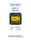
"Wavelet Spectrogram" shows a combined time/frequency representation of the impulse response. The Wavelet
Spectrogram in OmniMic uses a very fast algorithm that allows the display to occur in real time. In all time/frequency
displays there is a mathematical "uncertainty principle" which limits the degree of time resolution that can be obtained for
a given frequency resolution, and vice versa. In other words, the more detailed the time character of the display, the less
detailed will be the frequency character. The Wavelet Spectrogram shows the optimized presentation, giving as much
combined resolution as possible. The horizontal axis is time, the vertical axis is frequency, and color shows the relative
intensity (in dB). You can select the octave resolution, in a control below the plot, to determine the desired resolution
tradeoff. An ideal wavelet spectrogram (flat response, no resonances or reflections) will look like a vertical tapered horn,
like this:
15 | P a g e
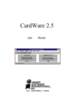
The time resolution is more detailed at higher frequencies than at lower frequencies (because there are more "Hz" in an
octave at high frequencies than at lower frequencies).
A typical loudspeaker will show a less clear graph, with smearing at various frequencies and additional color features
appearing at later times where reflection or diffraction occur.
16 | P a g e
If you spread the time axis out to full length, you can also use the Wavelet Spectrogram for viewing room reflections and
the frequency ranges over which they predominate.
Features of the Waterfall Displays
•
•
•
•
•
•
•
For CSD and TES type waterfalls, the top of the screen reference line is set by the largest feature over the
selected frequency range. Both types also allow selection of an "EQ flat" function that adjusts gain at each
frequency, as if an ideal equalizer were applied. Time is shown on the "depth" axis. You can click at the end of a
line trace on the labeled axes (time for CSD, frequency for Toneburst) to highlight the single line in a waterfall plot
for easier reading.
For CSD and TES, the position where you click within the Impulse Response graph below determines the length
of the waterfall calculation, starting from 0ms..
For the Wavelet Spectrograms, the red color indicates the highest decibel level in the frequency range. The "EQ
flat" button can be used so that red instead indicates the highest level at each frequency (in effect, what would be
obtained if the speaker could be equalized flat without affecting its phase). Impulse response windowing
will not have an effect on Wavelet Spectrogram displays.
The three dimensions (intensity, frequency, and time) of the graph can be adjusted as desired for display
using scaling controls similar to those on the other OmniMIc graphs.
As with the rest of the OmniMic graphs, there are buttons provided for both taking Snapshots of graphs or for
sending copies of the screen display to a printer (if installed on your computer).
Often selection of the Log format display of the Impulse Response graph below will allow for easier location of
strong reflections.
To return to the normal Frequency Response page of OmniMic, click on the "Return to FR" menu button.
17 | P a g e
Determining Z-Offset (depth offset) between speaker drivers
Index
A major advantage of Omnimic over other audio measurement systems is that it doesn't require a signal connection
between the computer and the audio system or speaker being measured. You can measure system response without
needing access to electrical connections simply by playing a test CD or audio file. That's very handy.
But there is a complication that comes with this convenience, which is that without a hard connection Omnimic has no way
of knowing the precise time at which a signal it is sensing left the loudspeaker. Omnimic determines timing by finding the
largest peak in the measured impulse response and referencing that in its phase determinations. When generating files
for loudspeaker design, it is important to know the relative delay between drivers in the loudspeaker system. If a
midrange driver is recessed in a baffle this will typically require a different crossover circuit than if the midrange is flush
mounted on a baffle. Different drivers have different amounts of depth, or "z position" of the originating point of the sound
waves they generate. What is important to know is not the absolute location of the acoustic origin of each driver, but the
relative "z offset" between two drivers for which a crossover section is being designed.
Omnimic now has a new feature to provide accurate determination of the z-offset between pairs of drivers. This feature is
based on a method described by Jeff Bagby for use with his PCD software, in which separate measurements are made
of each driver, and then those files are then combined mathematically and compared to a measurement that was made
with both drivers playing simultaneously. Bringing this process into OmniMic limits the number of files that have to be
exported from OmniMic to PCD and simplifies the steps for the user.
The feature uses a new math process for live ("Main") curve in Omnimic, which is a vector "Sum" function. This can be
found in the "Main Math" menu of the Frequency Response screen. When this is chosen (and an appropriate FRD file is
selected for summing with any new measured responses), the Main curve will be that of what is actually measured,
summed with the specified FRD file. For this to be reasonable, the saved FRD file must have valid phase information, so
make sure that the "show phase" checkbox is checked when saving FRD files to be summed with!
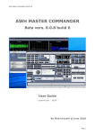
After a file has been chosen, a new menu option appears (see above), "Adjust Delay". Clicking this brings up a new form
with a control that lets you select the delay to be applied to the chosen file before it is summed with new measured
responses. If you check the box labeled "show Z-Offset Calculator", the form will expand to show a diagram and controls
which can calculate the proper Z-offset values to use in PCD.
18 | P a g e
________________________________________
How to use the Z-Offset Calculator:
•
•
•
•
•
•
•
•
1). Position your microphone at the design center point (often on-axis with driver "A", usually the higher
frequency driver, such as the tweeter if measuring a tweeter/midrange pair).
2). Make sure that "show phase" is checked on the Frequency Response screen. Measure the response of
driver "B" playing at moderately low level alone with the microphone at this position. Save this file to disk.
3). Connect so that both drivers "A" and "B" play simultaneously (use a blocking capacitor to protect tweeters, of
course, and be careful of levels -- these measurements need not be done at high level!) and save that to file also.
4). Use the "Added Curves">"Add" menu to add the newly saved file (of both drivers together) to the display.
5) Now go to the "Main Math">"Sum" menu and select the first curve (of driver "B" playing alone). Then click
"Main Math">"Adjust Delay" to bering up the form shown above. Put a check in its "Show Z-Axis Calculator"
checkbox.
6) Get out a tape measure and measure the distances shown in the figure (in either meters or inches), enter
them in the boxes. Enter an estimate for the distance from the baffle to the voice coil of driver B (this need not be
highly accurate, within several inches should be fine).
7) Uncheck the "show phase" box on the Frequency Response screen. Now, while measuring driver "A" alone
(the display of which is now summed with driver "B''s curve), adjust the control (in seconds) at the top of the new
form until the measured response curve best matches the magnitude (not necessarily phase!) of the Added Curve
that shows the actual measurement of both drivers together. When this is correct, then the value of Z axis offset
will be shown at the bottom right of the form. THIS (IN METERS) IS THE Z VALUE YOU WOULD ENTER FOR
DRIVER B in PCD, if driver A uses a Z axis position of 0.
8) Turn off the "Sum" function for Main Math, and measure (and save) the data from driver A playing alone for
use in PCD with driver B's curve taken initially.
19 | P a g e
Room Equalization with Omnimic
Index
Omnimic enables you to measure the frequency response of your room and speaker system at any number of listening
positions, weight the empahsis you want any of the positions to have relative to the others, and generate the required
response curve for your equalizer. The result can be the curve graph itself, or a set of parametric equalizer settings you
can enter by hand into parametric equalizers, or which can be loaded as a file to MiniDSP equalizers. These functions
are provided by the Equalizer Configuration form, which you can reach while on the Frequency Response page, by
clicking the "Main Math>Show Equalizer" menu.
The Equalizer Configuration form can't be shown unless there is an "Average" curve available in the Frequency Response
plot, which you can obtain from measurements as discussed below, or by loading an FRD file using the "File>Load to Avg
Curve" menu.
About Equalization
The frequency response of an audio system is not a constant, but will be different at each individual seat. Ideally we
would like the response to be flat (or some other target curve shape) at all seats from each speaker. But that isn't
possible in real rooms with real speakers because of the strong effects of loudspeaker directivity and sound reflections in
a room. So the best approach is to adjust the overall equalization to best smooth the response for all of the seating
positions, perhaps emphasizing the response at certain critical seating positions that are more often used. With Omnimic,
this is simple to accomplish, using its curve Average functions.
For instance, here is a graph with two responses from two different positions in a room:
20 | P a g e
If we equalized the response for flat at the Red position, then at 100Hz that would be fine for both Red and Blue around
100Hz. But Blue would end up with a big peak around 50Hz if it were bumped up as much as would be needed to make
the Red flat.
If we equally weighted the responses from both, we would get the Violet curve as shown below:
Averaging in Omnimic is "power averaging", meaning that peaks shown in dB carry more weight than do dips. This is
good, because peaks in response are more bothersome to sound than dips, so we want those to show stronger in the
curve we plan to correct from. Remember, if there is a peak in our Average curve, then during EQ we will be working to
pull the response down there with the equalizer's response -- peaks in room response become dips in equalizer response
to compensate.
But what if the Blue position is hardly every used, or is usually occupied by someone who doesn't care much about the
sound balance? In that case, we can just use more weighting for the Red curve as we develop our average curve. That
is simply done by introducing more averages from the Red position as for the Blue position. For instance, here is what the
Violet "Average" curve becomes if we used three averages from Red but only one from Blue:
You can see that the Violet curve now becomes a little more like the Red and a little less than the Blue.
21 | P a g e
Obtaining your Typical ("Average") Response Measurement
To make up your average curve, play one of the "Short Sine Sweep" responses from the speakers while measuring with
the Frequency Response tool. Set the "all, blended, only to" buttons to "all" (which will include all reflections in the
results) and the smoothing to 1/6th or 1/12th octave. Put the microphone at the first listening position and click on "New
Average" (or tap the spacebar on your keyboard). If you want to emphasize this, say, 5 times as much as the least
important seat, click or tap 5 times while there. Then repeat for all seats of interest. In a large theater, you can save time
and just do this for a sampling of seats in different general areas. The red curve on the graph that appears is the
"Average" response curve that you will want to equalize for. You may want to save this average response curve to disk
using the "File>Save Avg Curve" menu, which will allow you to reload it later should you wish.
Getting the Equalization Curve
Now, bring up the Equalizer Configuration form by clicking the "Main Math>Show Equalizer" menu. A small form will
appear.
In the form, you choose:
•
•
•
•
the frequency range over which you wish to equalize
the type of target curve: a flat line with a specified slope; or a curve from a text FRD file (which you can select or
even create on the fly from an included text editor). The target curve will appear on the Frequency Response
form in a thicker grey line.
the amount (in dB) to offset the target curve. You would normally set this one (visually, watching the grey line and
the red Average curve) to the position that requires the least work of the equalizers to approximate the target
curve.
The offset will normally be based on the response within the optimization range, you can also choose to "lock" it
so that frequency range selection doesn't further affect it or so that the same target can be used for different
speaker channels.
You would typically equalize an in-room response to approximate some "target" curve, which is the response
shape you wish the system to have. In many cases, the target will be a "flat" response, but possibly you may find
that using a "house curve" or a response with a slight downward slope will sound better with recorded music or
video programs. OmniMic makes this easy to achieve and to vary as desired. Equalization may only be desired
at bass frequencies in some systems.
If you need to generate an FRD or text file of the response curve, then at this point just click the "Make EQ
FRD file" button and tell the program where you want to store the file. This would be the approach to use if you
have only a "graphic" type equalizer available. Use the file to see the response your equalizer should ideally be
set for; approximation of this curve is usually sufficient, great detail in setting is not needed and is seldom
recommended.
22 | P a g e
The red curve above is an in-room measured curve, and the green curve is a generated EQ frd file (loaded as an
"Added Curve" and offset 60dB for display).
To obtain parametric equalizer settings, put a check in the box labeled "show parametric EQ filters" and the
form will expand to show:
Six sets of EQ section controls appear. Each section can be set to PEQ (parametric equalizer), High Shelf, or
Low Shelf, and can be set for manual mode, bypass, or automatic mode. You can select the effective frequency,
the "Q" (the ratio of center frequency to bandwidth), and the dB intensity of each. The result of applying all the
filters will appear as a gold curve on the graph.
For example, for each of 6 sections, you can apply a parametric filter to cut or boost a selected amound (in dB), at
a selected frequency, and with a selected "Q". Q is related to bandwidth. A lower-Q setting means that the boost
or cut will be effective over a wider range of frequencies, while a higher-Q setting will cause the effect to act over
a narrower range of frequencies with a sharper curve.
23 | P a g e
If you set any of the EQ sections to Auto, then the form will further expand to show buttons and limit settings that
the Omnimic program will use to automatically optimize the filters to approach the target response shape. Two
buttons are at the bottom of the expanded form, "Reset Auto values and Opt" and "Optimize from current values".
You would use the first if you want OmniMic to distribute the available filters over the range and start a new
optimization. You can use the second when the current settings (from a previous optimization or from manually
set values of certain sections) are to be used as the starting point for further optimization. You can interrupt
optimization at any time by using the "Stop Optimizing" button that will appear during optimization. The "err" value
is a number that shows the progress of the equalization, so you can tell whether the optimizer is "stuck" (and may
need some manual intervention) or is still making good headway. Often a better solution will be found if you stop
optimization and then restart with the "Optimize from current values" button several times.
The filter settings can be applied manually to parametric equalizer units (you may need to convert Q to Bandwidth
using the formula BW=Frequency/Q). For equalizers such as MiniDSP which accept biquad filter coefficients, use
the "View/Export Biquads" button to export a file which can be directly imported. See MiniDSP Equalizer Tuning.
24 | P a g e
MiniDSP Equalizer Tuning
Index
The OmniMic v4 software MiniDSP Equalizer function allows you to configure parametric filter settings, manually and/or
automatically, and view the result as applied to a Frequency Response in the Average Curve. The settings you
determine by this method can then be exported in a file from OmniMic, and then imported into the MiniDSP's control
program for downloading to MiniDSP hardware. You can adjust up to 6 of the MiniDSP PEQ or shelf filters at a time, and
then generate a parameter file for use by MiniDSP. Additional filters can be added, if desired in sets of 6 (before or after
the crossover filters, with Mini-DSP's "2-way Advanced" crossover, and some other plug-ins -- see MiniDSP's
documentation for details).
For example, for each of 6 sections, you can apply a parametric filter to cut or boost a selected amound (in dB), at a
selected frequency, and with a selected "Q". Q is related to bandwidth. A lower-Q setting means that the boost or cut will
be effective over a wider range of frequencies, while a higher-Q setting will cause the effect to act over a narrower range
of frequencies with a sharper curve.
You would typically equalize an in-room response to approximate some "target" curve, which is the response shape you
wish the system to have. In many cases, the target will be a "flat" response, but possibly you may find that using a "house
curve" or a response with a slight downward slope will sound better with recorded music or video programs. OmniMic and
MiniDSP make this easy to achieve and to vary as desired. When you adjust the settings for any of the filter sections, its
effect is immediately shown in an additional yellow curve on the plot, along with the unaltered "Average" curve.
When equalizing a room response, one of the errors that users often make is to "over-equalize", making tedious narrow
adjustments to flatten each dip and peak as seen at a very specific listening position. The problem with doing that is that
the response of a speaker and room is extremely position dependent. Ideally, you want an equalizer correction that
provides the closest approach to the desired response for ALL likely listening positions (as well as all sitting positions of
the listener!). This is why OmniMic has you adjust the equalizer based on the shape of the Average Curve. You can
obtain an overall typical frequency response measurement (an "Average"), as determined at all the listening seats, by
measuring the response at each and clicking the "New Average" or "More Average" button to include that data into the
ongoing Average curve shape (which will show in a red line). If you want to emphasize the response at any particular
seat (such as where you normally sit) to correct better for that position while stll considering the others, click the "More
Average" button several times after measuring at that position. You can alternately load a previously saved Average (or
standard) response curve using the File Menu ("Load to Avg", "Save to Avg"). You can also average in the most recently
added "Added" curve by right-clicking (rather than left-clicking) on the "More Average" button.
To bring up the equalizer control form, use the "Main Math">"Show Equalizer" menu from the Frequency Response
screen. You must have an Average Curve showing to bring up the Equalizer form, which initially looks like this:
Put a checkmark in the box labeled "show parametric EQ filters" and the form will expand to show:
Each Equalizer section can be set for "Manual" or "Auto" operation, or can be bypassed altogether. You can set the
mode of all six sections by using the master ("All") buttons at the top. In order to select the frequency, intensity, or Q of a
filter section, it must be in manual mode. You can adjust all the filters by eye, if you wish, or have the OmniMic software
automatically place and optimize the filters. Or you can set some of the filters only and let the rest be automatically set.
When you select any filter to use the automatic optimization, the form will expand to show additional optimization controls:
25 | P a g e
In the form, you choose:
•
•
•
•
•
the frequency range over which you wish to have automatic optimization occur
the type of target curve: a flat line with a specified slope; or a curve from a text FRD file (which you can select or
even create on the fly from an included editor). The target curve will appear on the Frequency Response form in
a thicker grey line.
the amount (in dB) to offset the target curve. You would normally set this one (visually, watching the grey line and
the red Average curve) to the position that requires the least work of the equalizers to approach the target curve.
The offset will normally be based on the response within the optimization range, you can also choose to "lock" it
so that frequency range selection doesn't further affect it or so that the same target can be used for different
speaker channels.
the maximum amount of boost you want the optimizer to attemp to use, to not overstress power amplifiers or
drivers in case of a severe response suckout. The limit can be specified as a fixed value maximum boost (for all
filters combined at any frequency) or as an FRD curve from a file (which you can again load or create on the fly).
you can also specify the maximum boost you want to have used by any individual filter section.
There are two buttons at the bottom of the form, "Reset Auto values and Opt" and "Optimize from current values".
You would use the first if you want OmniMic to distribute the available filters over the range and start a new
optimization. You can use the second when the current settings (from a previous optimization or from manually
set values of certain sections) are to be used as the starting point for further optimization. You can interrupt
optimization at any time by using the "Stop Optimizing" button that will appear during optimization. The "err" value
is a number that shows the progress of the equalization, so you can tell whether the optimizer is "stuck" (and may
need some manual intervention) or is still making good headway. Often a better solution will be found if you stop
optimization and then restart with the "Optimize from current values" button several times.
______________________________________________________
So, in summary, the steps for MiniDSP room equalization are:
26 | P a g e
•
•
•
•
•
•
•
•
•
1) Measure the frequency response (probably without windowing, using the "All" radio button above the plot) and
perhaps 1/6th or 1/12th octave smoothing. Make a number of measurements at different location and average
them into the Average curve. See: Room Equalization.
2) Open the Equalizer and use shelf sections to manually adjust the upper or lower ends of the response, and
possibly to fix obvious peaks. Set the other filter sections for Auto.
3) Set the frequency rang for the automatic optimization
4) Set the target curve shape as desired (a -0.25dB/Octave downward sloped curve is usually a good-sounding
choice), and adjust the offset for best fit.
5) Set any boost limits you may desire. A 6 or 7dB limit (or lower) is a good idea usually.
6) Click "Reset..and Opt" or "Optimize.." to start the process.
7) Stop when you are satisfied, or when equalization has run out of gas, or to change some settings before
optimizing some more with the "Optimize..." button.
8) When you are done, click on the "View/Export Biquads" button to bring up a display of the values that will be
exported to a file for MiniDSP. Save it to a file, and then import it into MiniDSP for loading to the equalizer
hardware.
9) Check the response at various seats to see the general improvement, then do some listening.
27 | P a g e
Polar Displays
Index
Polar displays are an Advanced Feature, provided by a non-live postcalculation using multiple saved
frequency response data files "Add-ed" to the OmniMic Frequency Response screen. The files must
have angle values assigned to them, and there must be at least three "Added" files present with
different angles assigned in order for a calculation to be possible. In general, seven or more files
should be used for good results. When you click the "Polar Display" button, the OmniMic system will
pause (halt incoming live measurements) as the Polar Display calculations are very intensive and
would interrupt live processing.
The purpose of a Polar Display is to reveal how the frequency response of a loudspeaker varies with
horizontal or vertical angles from the baffle. Speaker designers generally design loudspeakers for a
specified (usually, flat) frequency response at a position on-axis of a speaker and at some assumed
distance from the baffle. But such a response is not what a user actually hears in a real room -though some sound that projects at off angles isn't initially aimed at a listener, that doesn't mean that
its effects won't be heard. If you point a speaker away from you, you will still hear it very nearly as
loudly than as if it was pointed at you. You may hear it a few milliseconds later, but it will certainly not
be insignificant. Usually, most of the energy you hear from a speaker actually wasn't initially directed
at you, but is reflecting from around the room before reaching you.
Research shows that users generally prefer that the spectrum of reflected sounds should resemble a
flat (or smoothly decreasing) response relative to that from the directly arriving sounds. This has
resulted in interest in the polar radiation patterns of loudspeakers, and in designs intended to address
28 | P a g e
these patterns -- dipoles, omnidirectional, bipole, arrays, or waveguides.
To see the response magnitude (dB) varying with both frequency and radiation angle, a 3dimensional graph is required. OmniMic provides two versions:
•
•
A "flat" format, as shown above. In this format the horizontal axis is frequency, the vertical is
radiation angle, and the color represents corresponding dB level. An index relating color to dB
levels is shown to the right of each plot.
A "cylindrical" format, in which frequency is the vertical axis, the angle around the projected
cylinder is radiation angle, and both color and distance from the cylinder axis represent dB
level. The colored region of the graph can be rotated using provided buttons to give a more
intuitive view of the response shape than is obtainable by colors alone. This format can be
time consuming to process, so the "density" can be selected to trade-off graphic quality versus
time. Smaller form sizes for the plot also take less time to calculate, so you may wish to drag
the Polar form to a small size.
The graphs assume that the highest level in the included frequency range (of all included
curves) is displayed as "0dB" (red). If you are investigating a driver (or horn, or waveguide)
that hasn't been equalized (or voiced in a crossover), it is best to select the
"Curves>Normalize" menu and choose one of the curve angles to reference the others from.
The result would then be the pattern you could get were you to perfectly equalize the response
as seen from that angle. Typical normalization angles are for 0 degrees or 22.5 degrees (for
toed-in waveguides).
Normalizing the responses, however, can result in some apparently large peaks at frequencies
where the reference curve has low output. Such peaks would dominate the "0dB" value, so
you may want or need to adjust the frequency range of the polar plot to avoid ranges where
29 | P a g e
these peaks appear.
There is a set of example FRD files which can be loaded all at once by going to the Frequency
Response menu "Curves>LoadCurveList", then browsing
to C:\Users\Public\OmniMic\SEOS15 Examples and loading "All Curves". After loading
this, click on the Polar button to see the effect. Then try normalizing the files by going to
"Curves>Normalize", then browsing to the same directory and choosing one of the curves (the
22.5 degree curve is used for some of the illustrations on this Help page). Adjust the
frequency range of the Polar Display and note the effects -- if the lower frequencies below
700Hz (which are full of artifacts in the example), or the frequencies above 17kHz (also full of
normalization artifacts) are included, the artifacts will dominate the display's 0dB level. Adjust
the frequency ranges to exclude these. The result should be approximately the effects of
(hypothetically) equalizing the speaker's response to be flat at the normalization angle in that
frequency range.
Making Measurements for Polar Displays
For good quality Polar Displays, echoes should be minimized in the measurements. Set the
speaker out in a clear area so that reflected signals are delayed as much as possible. This will
allow them to be avoided at higher frequencies (see "Only To" and "Blended" in Frequency
Response ). Either the microphone stand or the speaker can be moved to arrange for each
angle for measurement. Steps of approximately 7.5 degrees or less are preferred for good
detail. The program will interpolate between the steps, and if only positive (or only negative)
angles are given, will mirror the measurements to the opposite side (this will be accurate, of
course, only for symmetric speakers or drivers). Try to measure out to at least 75 degrees
from the baffle axis on each side -- unmeasured positions will not be represented in the plot.
Dipole or Bipole speakers should be measured a full 360 degrees.
Name each file so that you can identify the angle it was measured from -- if you include the
number in the file name, the OmniMic software will try to infer the angle from the file name
when you later bring in ("Add") the files to a frequency response page.
Tip:
If you save the files by right-clicking on the graph and then choosing "Save Curve to Text File
(auto-increment)" then the program will automatically name each file by incrementing a number
in the file name.
30 | P a g e
You can configure the base file name and the increment value (and starting value) by choosing
"configure auto-increment".
Then, doing each curve, naming it and saving it is just a matter of right-clicking a few times
between each angle change of the speaker/microphone arrangement.
Be sure to save the collection of Added files to a File List after assembling them, for easy
future retrieval of the set!
A grid/protractor tool to assist in arranging angular measurements can be printed from the Help
page at Polar Protractor.
31 | P a g e
Polar Protractor
Index
Provided to assist in arranging OmniMic and loudspeakers when collecting responses for Polar Displays. Print this to a
sheet of paper and place at the speaker position.
32 | P a g e
SPL/Spectrum
Index
Use the SPL Meter/Spectrum Analyzer type to see -
The level of any sounds on the SPL meter face.
Options:
•
•
•
•
•
•
•
•
•
Select the meter damping type: Impulse, Fast, Slow or Slowest.
Read the Peak, Maximum or Minimum values sensed since the Reset button was last clicked
Choose the response weighting to use at the top of the tab page: A, B, C, or None.
When A weighting is selected, you can read the Sound Exposure Level (SEL) over time spans
starting from a click of the Begin circle to a click of the End button.
The spectrum of any sounds, on the Spectrum Analyzer graph.
Options:
Choose the FFT format for display in terms of "Hertz" frequency bandwidth. This format
allows you to choose the amount of smoothing applied.
Choose the RTA format for display in terms of "octave" frequency bandwidth. Display will be
separated into 1/6th octave bands.
Choose the response weighting to use at the top of the tab page: A, B, C, or None.
Don't use the Spectrum Analyzer to measure frequency response -- the Frequency
Response analyzer is much better for that function!
You can select the damping type for either analyzer graph from: None, Impulse, Fast, Slow or
Slowest
33 | P a g e
34 | P a g e
Oscilloscope
Index
Use the Oscilloscope to view any sound waveforms. These might include music, your voice, or
waveforms played by loudspeakers.
You can choose to trigger each "sweep" from the point where the acoustic pressure level rises or falls
past a selected acoustic pressure levels. To select, click the mouse on the graph at the desired level.
This makes display of repeating waveforms easier to see. To make the trace free-run, click
triggering to "off".
•
•
You can freeze the oscilloscope display to better examine a captured waveform by using the
Pause button (two vertical bars) near the top left of the OmniMic screen. Click the Play button
(forward arrow) to begin the display again.
If the waveforms being examined are cluttered with subsonic noise in the room, select the
"10Hz High Pass Filter" checkbox above the graph to remove the lower frequencies from the
display.
35 | P a g e
Signal Generator
Index
With most computers, Omnimic can be used to directly generate test signals such as the sweeps for Frequency Response
or Harmonic Distortion. The signal is generated from the computer's soundcard output, which can be connected via
cabling to other amplifiers or audio systems.
When Omnimic is used in the SPL/Spectrum mode or Oscilloscope mode, it can also generate sinewave or squarewave
test tones. To use this function, select the "Config">"Generator" menu and this form will appear:
There are two tone generators included, either (or none) of which can be used simultaneously.
Tone1 can be either a sinewave or a square wave of any audio frequency and is always at a fixed level -- this level is the
same (when a sinewave) as the level at which sweep tones are ouptut from the soundcard when sound is played out in
the Frequency Response, Distortion, Reverb or Bass Decay.
This provides a handy way to provide known signal level to loudspeakers under test. With Tone1 set to about 55Hz,
sinewave, and applied to a power amplifier (which is in turn connected to an AC Voltmeter or DVM set to AC Voltage
mode), adjust the amplifier's volume control to the desired voltage level. For loudspeaker sensitivity measurements, this
is normally a voltage level of 2.83Vrms (equal to 1W into an 8 ohm load). Then change over to the Frequency Response
page, connect the speaker, and with the soundcard again providing the test tone measurements will be at the 2.83V
standard level.
Squarewave mode with Tone1 can be used to view (on the Oscilloscope) the response of speakers to a square wave. Be
aware, however, that very few loudspeakers can produce a recognizeable squarewave over any range of frequencies.
There is little if any evidence that this is actually important sonically, but the characteristic can still be interesting.
Tone2 is always a sinewave, and both its level and frequency can be adjusted as desired. Its output level (in dB) is
relative to the level of Tone1, that is, when the relative level is set to 0dB, then Tone2's level is the same as Tone1's
level. Application of the two tones simultaneously can be used to conduct single frequency-pair intermodulation tests of
loudspeakers, viewing the level of intermodulation product frequencies on the FFT Spectrum Analyzer (in the
Spectrum/SPL page). When doing this, however, be aware of complications from sound reflections in the room -- such
tests are best done with the microphone close to the speaker (if the total SPL level is less than about 110dBSPL) or
outdoors where reflections can be avoided.
36 | P a g e
Harmonic Distortion
Index
To properly measure Harmonic Distortion with OmniMic, you must measure only while the sound
system is playing one of the provided "Long Sine Sweep" tracks of the OmniMic Test Track CD.
Use of other sound signals will not provide meaningful results.
•
•
•
•
•
•
•
•
•
•
This measurement will work best when the OmniMic is positioned relatively closely to the
loudspeakers, so that sounds coming directly from the speaker are much stronger than those
coming reflected from elsewhere. Room reflections are very detrimental to measurement of
harmonic distortion.
The microphone and speaker should be held stationary over the length of several of the test
sweeps (approximately 6 seconds each) previous to each graph update
At very high levels (>125dB SPL), appreciable distortion may be generated from overdriving of
the OmniMic itself.
When you position the mouse cursor over a distortion graph, a small box will appear displaying
the frequency, SPL level, and effective Harmonic Distortion percentage of the overall SPL,
relating to the position of the cursor.
You can freeze the graph to read multiple positions by using the Pause button near the top left
of the OmniMic screen.
The graph will always display the frequency response curve (in dark black) at top, indicating
the effective SPL level sensed at the position of the OmniMic. In addition, the graph can be
configured to display
2nd Harmonic Distortion level
3rd Harmonic Distortion level
4th Harmonic Distortion level
5th Harmonic Distortion level
2nd through 5th Harmonic Distortion levels (Total Harmonic Distortion for the first 5 products;
for loudspeaker distortion these harmonics normally are the highest)
37 | P a g e
38 | P a g e
Reverb/ETC
Index
Reverberation is a measure of how quickly sound reflections die down in a room, and will depend on
the frequency range of the sound, the size and shape of the room, what is in the room, and how the
room surfaces are constructed. Determination of RT60 can be made using this tool.
ETC stands for "Energy-Time Curve", which is a similar display, but which shows individual reflection
spikes more clearly to help in locating where they are coming from. This display is also able to
calculate "Speech Transmission Index" (STI) for auditorium and hall acoustics evaluations.
A third display option "Log IR" shows the dB level of the Impulse responses (like the one at the
bottom of the Frequency Response tab page, but in a decibel format), a very similar result to the ETC
in most cases.
These tests must be done while the sound system is playing the "long sine sweep" tracks of the
OmniMic Test Track CD . Use of other sound signals will not provide meaningful results.
Reverb (RT60)
OmniMic provides a graph of the reverberation decay curve. A properly done reverberation decay
curve will drop 40 decibels (dB) or more, relatively smoothly, from left to right. Using the mouse
cursor on the graph and the mouse button, you can obtain a measure of the RT60 value -- the time
needed for a reverberant field to die down by 60 decibels.
39 | P a g e
•
•
•
Set the value of the "Integration time" to a value approximately equal to the expected RT60 of
the room (around 500 milliseconds typically). The optimum value is the one that makes the
decay line the straightest and longest.
Set the lower and upper frequency limits to define each frequency range over which you wish
to measure. The width of the range will be displayed in Hz and in Octaves. If you wish to
force the controls to hold current number or octaves of range, click the small "lock" icon and
the controls will track accordingly. Click again to unlock.
Click on the graph to define a line parallel to the decay curve. The slope of this curve defines
the value of RT60, which will be displayed on the screen until the next graph update. This may
be easier to do if you first freeze the graph with the Pause button at top left of the OmniMic
screen.
ETC (Energy-Time Curve)
The curve shown is the energy relative to the level of the energy in the first peak as an impulse
40 | P a g e
comes from the speaker and reflects around the room. In other words, imagine the speaker
sent out a sudden pulse rather than the sweep this test uses. (OmniMic calculates results
equivalent to a pulse using a sweep as the sweep is better at rejecting noise and distortion).
The first spike in the ETC is the original at 0dB and 0msec time, usually a direct signal from the
speaker. The following ones are as reflected from the various surfaces around the room. You
can often hold a piece of acoustic absorber (acoustic tile or even a pillow) near surfaces near
the speaker or microphone to identifiy the sources of reflections. The controls at the top of the
form allow you to filter the ETC to include only certain frequency ranges.
Omnimic can now save and recall (as Added ETC curves) ETC measurement files,
allowing multiple curves to be shown simultaneously. Curve files can also be smoothed before
saving, to help in interpretation.
When in ETC mode and operating with full bandwidth, you can also have Omnimic calculate
the "Speech Transmission Index" (STI) or the "Rapid Speech Transmission Index" (RASTI,
a similar but less intensive version). To use this play the long sweep test signal from the
system being tested (typically a public address or theater sound system) and put the
microphone at the seating positions. It may take several sweeps for the STI or RASTI to
appear. These are very intensive calculations, so the update rate will generally be slowed
when calculating STI or RASTI. A result of "1" is perfect, "0" would be worst that could be
expressed. Good signal to noise is desirable when making the measurement, so use sufficient
test level.
41 | P a g e
Bass Decay
Index
Use the Bass Decay analyzer to measure how bass notes decay in a room.
•
Use only the provided "bass sweep" tracks to perform this test. Other signals will not
provide meaningful results.
When a bass note is stopped within music, the sound in the room at some frequencies may
still continue for some time. That is because the sound reflects back and forth between walls,
resonating and forming "modes" before eventually dying down. This is not altogether bad and
some reinforcement is normally desirable for natural sounding playback, but you would like to
keep it under control and not have some notes sounding muddy or lingering much longer than
others.
The top graph on the Bass Decay display shows the frequency response of the bass range,
similar to that shown with the Frequency Response analyzer. The bottom graph shows how
long it takes the sound to decay at each frequency. As shown on the legend to the right of the
decay graph, the white area extends upward to indicate when the level drops no more than 5
decibels (dB). The light blue indicates when the level has dropped between 5dB and 10dB,
etc.
42 | P a g e
At the bottom is a check box labeled "adjust for response". This affects whether the
variations in relative bass strength are included when calculating the the decay graph.
•
•
when the "adjust for response" box is unchecked, the bass decay shown does not take the
frequency response into accout. All decibel levels are with respect to whatever the response
level is at each frequency. At frequencies where there is lower overall output (as shown on the
upper graph), the decay may appear to be longer than actual because of background noise in
the room that is inseparable from the low bass levels.
when the box is checked, the decibel levels are with respect to the blue line shown on the
frequency response graph. For instance, if the line is at 70dB SPL, then the white area of the
Bass Decay graph shows how long it takes before the level dropped below 65dBSPL (that is,
70dBSPL minus 5dB), the light blue shows how long before the level dropped to 60dBSPL,
etc.
43 | P a g e
Operating Notes:
•
•
•
•
when working with the "adjust for response" box checked, you would normally set the blue line
(click inside the Bass Response graph) to be in the upper, most flat, region of the Bass
Response curve.
the microphone should be placed out in the room, measuring at various listening positions.
You can try relocating subwoofers or main speakers, or listening chairs to find optimum
locations for these. For floor vibrations, spikes or pads below subwoofer boxes can also affect
the bass decay (not always for the better).
remember that the response is strongly position dependent. Optimize the woofer placements
and equalization for best overall results at all listening positions. This is generally easier to
accomplished if multiple subwoofers are used.
slow decays should be less bothersome to the ears if response level is reduced at the
problematic frequencies. If you are using an equalizer in the room, you can reduce your
system's response to accomplish this. You can use the "adjust for response" checkbox to help
find the best tradeoff between tight bass and flat response.
44 | P a g e
Scaling Graphs
Index
The various graphs and the SPL meter display can be scaled as suits the user. Or they can be set to
automatically scale (vertically or meter range).
Each graph has several arrow buttons that, when clicked, will adjust some of its coordinates.
These compress or expand the curves vertically
These move the curves up or down vertically. You should turn off automatic scaling if you
want to adjust these manually
These adjust the horizontal value of the left or right borders of the graph
Automatic scaling will be temporarily disabled whenever the mouse cursor is over a graph, to keep it
stable while reading data point values.
In addition, the entire OmniMic panel can be scaled as desired, all the way to a full-screen view.
45 | P a g e
Adjusting Input Gain and Auto-Level
Index
For best results, the input sensing gain of OmniMic should be adusted approximately for the sound
level. The input gain slider control is at the top right of the OmniMic screen.
•
•
•
The slider should be set so that gain is not too low (which would limit dynamic range) and not
too high (which would overload OmniMic's electronics).
When a sound level is sensed that is too high for the OmniMic, a message and a small red dot
will appear to the right of the slider -- if you see this, move the slider to the left to reduce the
gain until the red dot no longer appears.
The gain can instead be adjusted automatically by the OmniMic software if you temporarily put
a check in the small box next to the slider. Expose the OmniMic to the sound level that will be
used for several seconds, and the slider should adjust to a compatible level.
It is best NOT to leave the auto gain button checked during measurements, since the
slider movement can interfere with ongoing measurements.
46 | P a g e
Freezing the Graphs
Index
By default, the OmniMic software runs, and the graphs and meters update, continually. At times you
may wish to keep a graph steady for inspection or for reading off data points using the mouse cursor.
This is simply accomplished by clicking the Pause button at the top left of the OmniMic screen.
To set it running again, click the Play button.
47 | P a g e
Reading Values on Graphs
Index
You can position the mouse cursor on most graphs to read data values that would exist at the point
that represented vertically and horizontally. While the cursor is placed there, auto scaling will be
temporarily disabled. Move the mouse cursor outside of all graph areas to allow the graphs to
autoscale (when autoscaling is enabled).
48 | P a g e
Printing Graphs
Index
Print the current OmniMic screen image by clicking on the Print menu. You can select the printer that
will be used via the "Printer Setup" menu on the main OmniMic screen. On most plots (not including
Waterfalls or Polar displays) you can also print from a pop-up menu that appears when you right-click
on the graph.
When a frequency response graph is shown with multiple curves (from files), the image that will be
printed includes an extra column at right indicating the files used for each curve. Because of the
limited space for showing the file names, short file names are recommended.
If you want to print only an individual graph (without the buttons or controls of the rest of the image),
you can get a very clean copy of it by using the "Snapshot" menu, and using a graphics program
(such as PaintBrush) to print the image.
49 | P a g e
Saving Graph Pictures to Disk ("Snapshot")
Index
You can save a high quality picture file of the current graph by clicking on the Snapshot menu. These
are useful for including into reports or published documentation, or for printing out separately using a
graphics program (such as PaintBrush). Buttons and controls shown on the graphs will not be saved
to the file. However, if you have multiple curves (from data files) on a Frequency Response plot, a
legend will be included in the graph identifying the curves with the files.
On most plots (not including Waterfalls or Polar displays) you can also command a snapshot from a
pop-up menu that appears when you right-click on the graph.
You will be prompted for a file name. Files can be saved as bitmaps, PNG files, JPGs, or as scalable
metafiles. Metafile displays can be scaled smaller or larger (when used with capable software like
most word processors) without loss of resolution. Bitmaps are more universally supported, but may
not expand or compress as well when inserted into documents. JPGs are ideal for posting on internet
web sites or discussion boards.
50 | P a g e
51 | P a g e
Saving Data Files to Disk
Index
Data files can be saved to disk by clicking on the File menu. It will be saved in an ASCII text format
which can be imported into a spreadsheet program if desired.
Frequency response data (".frd") files saved this way can be reloaded back into the OmniMic program
display using the Curves menu. Curves may be loaded individually or a list of curve files can be
loaded or saved for fast recall of a group of curves.
You can also select a data file save operation for most plots (not including Waterfalls or Polar
displays) from a pop-up menu that appears when you right-click on the graph. For Frequency
Response plots, there are also options for easy auto-incrementing file name generation for making a
series of related measurements, particularly helpful when you are collecting curves for a Polar
Display.
To save in impulse response as a WAV file, right-click in the Impulse Response (lower) plot in the
Frequency Response page. The time length of the saved file will be about 620msec, at a sample rate
of 48kHz.
The data curve reloading feature is available only for Frequency Fesponse and ETC files. Other type
files should be saved as graphic snapshots if the plots are required later.
52 | P a g e
Playing OmniMic test tracks without a CD
Index
OmniMic test tracks can be "ripped" from CD using commercially available software for playback from
a computer soundcard or other player as WAV files.
A test DVD is being planned, which can provide test signals to individual channels in a 5.1 surround
system.
In many cases, the tracks can alternately be saved as MP3 files for playback from computer systems
or MP3 players. If using MP3, use one of the higher quality type MP3 compression formats (128k or
better) for best results. Some ripping programs may do better than others in providing usable MP3
test tracks. For Frequency Response measurement using MP3, the Sine Sweep track will usually
work better than the Pseudo Noise track.
Use of MP3 format is NOT recommended for making Harmonic Distortion measurements.
53 | P a g e
Instructions for special measurements not described on other pages
Index
How to...
Splice two or more frequency response curves together in a graph
This can now be easily done using Added Curves. Just save the responses to FRD files, then use the "Added
Curves">"Add" menu to bring in both curves, selecting them to have the same color. Configure their frequency ranges so
that one ends where the other starts. If you need to readjust either of them, just select the "Added Curves" menu and
click on the curve name at the bottom of the offered submenu to bring up the properties form for the Added Curve.
Is there a fast way to disable sound output when I'm using the computer to generate test
signals directly from Omnimic?
Yes, simply press on the [Esc] key on your keyboard. Press [F2] to start it again.
Point the microphone
Omnimic is a small capsule, narrow tip measurement microphone and its response is essentially omnidirectional at most
frequencies. At very high frequencies, there is about 3dB reduction in response at 13kHz, as can be easily determined by
making a set of comparative measurements with the mic pointing at and then perpendicular to a high frequency speaker.
Here is a result of such a measurement (showing the effect of perpendicular to directly aimed response):
Align two speakers in "time of arrival" at a listening position
Arrange your system so that the Test Track sound plays out of both speakers you are working with, but with any other
speakers silent. Choose the Frequency Response page and play the indicated track with the microphone set at the
desired position. Set the control that is near the top to "blended" and observe the Impulse Response display. If there is a
time of arrival difference between the two speakers, you should be able to see two impulse peaks. The one to the left
(near the 0 msec point) is from the speaker with the earlier delay time, the other is for the later one. If you have an
electronic delay unit, adjust the delay applied for the earlier speaker so the peaks become superimposed. If you have
more than two speakers you wish to align together, choose the latest (the one making the right-most peak) to be the
reference and delay the others to align to its peak
54 | P a g e
Optimally position speakers within a room
Speaker and listener positioning within a room is probably the most significant factor determining how a system will
sound. This can usually be best adjusted using the Frequency Response display and either the Pseudo-Noise or the Sine
Sweep signal. Set the control near the top to "All" for a display in which all echoes, reflections, and room effects are
included and apply 1/3rd octave smoothing. Start with one speaker playing at a time. The response will normally be
irregular, but try moving the speaker position or listening position for the most uniform response, particularly at lower
frequencies below 200Hz. For stereo, you will need to find two locations which can give a good stereo image together
while optimizing the low frequency response. Very often such factors are not mutually attainable. Low frequency
positions may also be optimized to minimize standing waves by use of the Bass Decay analyzer.
A strong advantage of using separate subwoofers (rather than only full range speakers) is that they allow you to optimize
the mostly non-directional subwoofers for smoothest bass response and the upper frequency speakers for best stereo
imaging. While bass tends to be nondirectional, the in-room response of the bass speakers is extremely sensitive to
placement. You will almost always be able to get the smoothest overall low frequency response by using two or three
subwoofers optimally placed in different parts of the room, rather than a single subwoofer - even if the single subwoofer
were of much higher quality. The room position and diversity of placements will have significantly more effect on bass
frequency response than could subwoofer response flatness.
Adjust an Equalizer
Omnimic now has a very sophisticated feature for manually or automatically configuring an equalizer, and downloading
settings to MiniDSP type equalizers through its Biquad Parameters.
When adjusting equalizers:
•
•
adjustment at lower frequencies should use a measurement setup similar to the one for positioning speakers (but
the placement should be determined first). Strong boosts with the equalizer should be avoided at any frequency,
but response peaks can be effectively removed to any degree necessary.
Equalization at higher frequencies are usually best done only in moderation, and generally adjusted with echoes
removed by setting the Frequency Response analyzer to "blended" and clicking the mouse within the Impulse
Response display on a point just before the first strong reflection. Avoid sharp narrow-band adjustments on the
equalizer at higher frequencies because they can cause significantly worse sound at slightly different listening
positions.
Adjusting for more than one listening position
For theaters or other situations with multiple listeners, compromise settings must be made to provide the best
sound overall for all listeners. Begin by optimally positioning the low frequency speakers (or main, if full range) to
avoid major problems at various seats, particularly those furthest from the center. Again, use of several wellplaced low frequency speakers will be most effective for giving good results for all listeners.
Then, with the Frequency Response analyzer set to "All" and with 1/6th octave smoothing use
the Averaging features. Make a series of measurements at all (or at least a good representative number) seats,
starting with "Clear Averages" then "New Average" for the first, and clicking "More Averages" (or pressing the
spacebar) once with the OmniMic placed at each position. This will result in an overall average room frequency
response, which you should save to disk or print for future reference. You can then adjust your equalizer to
provide approximately the opposite of the resulting response; the new Equalizer Configuration form makes this
easy. That is, if there were an 8dB peak (relative to response at most frequencies) in the 4kHz range, then if a
flat response is desired, then the equalizer should be set for -8dB at 4kHz. Avoid applying large increases (more
than about 6dB) with the equalizer and use only moderate and broad (not sharp in frequency) settngs at
frequencies above about 500Hz.
55 | P a g e
Arrange and test whether a frequency response falls within a specified range
The "Evaluate within" function (in the "Math" section of the Frequency Response menu will show a small rectangle
at the top left of the frequency response graph that indicates whether measured responses fall within ("good") or
outside ("out") of the first two curves specified in the Curves menu. The evaluation is performed only over the
frequeny range currently being displayed. To use this to determine whether new measurements fall within (for
example) 3dB of a reference measurement, first make the reference measurement and save it to disk using the
"File->Save Curve" menu. Then, in the "Curves" menu, choose "Add" and then select the file you just saved and
then select an offset of 3dB on the form that appears. Use the "Curves->Add" menu again to choose the same
curve, this time with an offset of -3dB. The two curves should show on the graph. Next, go to "Advanced Mode"
(if you aren't already there) using the checkbox provided and in the "Math" menu, select "Evaluate within". You
can select whether to allow the program to try to fit the curve by shifting it up or down by up to some maximum dB
value. Finally, set the frequency range of the graph (using the yellow arrow buttons) to display the frequencies
over which you wish the evaluation to be performed.
You can alternately define the two curve files to be used for limits by generating them using a text editor (simply
load an FRD file into your text editor to see the simple format. All frequencies need not be present, but they do
need to be in increasing order). Users familiar with spreadsheets such as Microsoft Excel can use these to edit
FRD data for special custom limit curves, after resaving the resulting data with an FRD extension (or saving with a
.txt or .prn extension and then changing the extension to .frd).
Measure frequency responses of Tweeters
OmniMic normally tests loudspeakers with a full range signal that briefly passes from below 2Hz to above 20kHz.
Some speaker drivers, particularly tweeters, compression drivers, ribbons, or electrostatics cannot be safely
driven at low frequencies. When testing devices such as these, you should always drive them through series
capacitors (at least) to limit low frequency drive. You can calculate the approximate value to use as
C=1,000,000/(6.2*f*Z) where f is the desired cutoff frequency, Z is the driver impedance, and C is the value in uF.
Smaller values of capacitor are safer
.
Using such a capacitor causes a problem, though -- it also affects the measured response. If you test with a
cutoff capacitor that acts far below where you tend to use the speaker then those effects might be ignored, but in
that case you would be less protected.
Another option is to test with a pre-filtered (but still syncrhonous with OmniMIc) signal that has a known highpass
response. Several of these are provided on the V3 CD (or DVD) test disks, some with "bass removed" and some
with "bass and midrange removed". The "bass removed" tracks roll off below 300Hz, and the "bass and midrange
removed" tracks roll off below 3kHz. The effect of the rolloffs from using these tracks can be corrected by
Normalizing the measured responses (either at measurement time, or after Adding an uncorrected file) with either
the "Bass Removed.frd" or the "Bass and Midrange Removed.frd" files that can be found in
your C:\Users\Public\OmniMic folder.
IMPORTANT NOTE: You should still use a series capacitor (perhaps something large such as 100uF) to
protect your sensitive driver from transients, hum, or other signals from the setup which might cause damage.
Note, however, that when you use those test signals, the measurements will be much more susceptible to noise
below the rolloff frequencies, so you should adjust the diplayed frequency range above the lower frequency
range.
Measure sensitivity of loudspeakers
Loudspeaker sensitivity is normally expressed as the SPL level that is sensed at 1 meter from the loudspeaker
when it is driven from a voltage of 2.83Vrms. When you are using a CD as the signal source with OmniMic, the
nominal level of the swept sine signals can be determined (or set) by use of the 50Hz reference tones that are at
the end of the Version 3 OmniMic Test Signal CD or DVD.
To use these, you may want to disconnect the speaker of the channel being tested (the output voltage of quality
amplifier should not be affected by whether a speaker is being driven). Then attach a Digital Voltmeter (also
known as a "DVM") to read AC Voltage across the amplifier terminals. Be sure to configure the voltmeter for AC
Volts and that the probes connect to the meter's Voltage (and not its Current!) reading terminals.
56 | P a g e
Turn any equalizer or tone controls off. You can then play the 50Hz reference tone tracks and measure or set the
voltage level from the amplifier. Next, reconnect the loudspeaker, set OmniMic at the 1 meter distance from the
loudspeaker and play the desired sweep track of the test CD. Use the OmniMic software in its Frequency
Response measurement mode for Sine Sweep, and the plot should then be a reading of SPL sensitivity.
Some loudspeakers reference to a 1 watt level rather than to a voltage level. 2.83Vrms is equivalent to 1 Watt
into an 8 ohm (resistive) loudspeaker. For a 4 ohm loudspeaker at 1 Watts, the voltage to use would be
2.0Vrms, for a 16 ohm speaker use 4.0Vrms.
getting FRD files for crossover simulations
Designing a crossover is much easier if you can do it using simulations rather than by trial and error and physical
parts. To design via simulation, you need to have both magnitude and phase responses for the drivers you will be
using. For passive crossovers, you will also need impedance data for the drivers -- for that, an electrical
impedance measurement such as the Woofer Tester 3 is ideal. See "Determining Z-Offset" for a technique
that provides accurate phase responses for crossover designs using PCD and similar programs.
You can also do the adjustments within the PCD program using files made with OmniMic. For this you need three
measurements of each pair of drivers -- one of each driver alone, both with phase response, and one of both
playing together (without a crossover, which isn't designed yet). You should use a blocking capacitor on the
tweeter to avoid hitting it with very low frequency energy, and you should also keep the test level down to the
lowest level that provides a clean measurement. The phase response can be made using OmniMic in its
"Advanced Mode" and with phase enabled, but without any "added tweeter" -- this gives a true phase response
measurement, though the delay between driver and microphone isn't accounted for -- and that is what Jeff's
technique addresses. For the measurement with both drivers playing, try both with the tweeter inverted and with
it non-inverted to try to find a configuration which gives a null where both drivers are playing. Then using the
measured response FRD files from each of the individual drivers, simulate in PCD the results of both playing (and
with the tweeter polarity as used for the combined measurement). In PCD, vary the simulated delay between the
two drivers to make the results (in dB curve shape) match as closely as possible the shape of the dB curve
measured when both drivers were playing. This delay value then will correct the relative delay between the two
drivers for complete crossover design in PCD.
57 | P a g e
Troubleshooting
Index
Listed are answers to some questions that may arise.
There is a message with a yellow background telling me "Check for Correct CD Track!".
Most tests with OmniMic (other than "SPL/Spectrum" and "Oscilloscope") require particular CD tracks
to be played on the system that you are measuring. The tracks contain test signals necessary for the
OmniMic software to do its analysis. You cannot substitute other test signals. For example,
although the "Pseudo Noise" (CD Track 1) signal sounds like pink noise, it is actually very different
and use of pink noise in its place will not produce a useful result. The proper CD track to play for any
OmniMic test is displayed at the top of the OmniMic screen. If you have lost your OmniMic test track
CD, contact your Dayton Audio dealer or check the Dayton Audio website for a replacement.
In most cases, it is also possible to play copies of the CD tracks that have been recorded to other
media, see Playing OmniMic test tracks without a CD.
I get messages saying that my "Control Panel" settings are not correct for OmniMic.
This can happen in Windows VISTA or Windows7 (and possibly in later Windows operating
systems). For proper operation of OmniMic at higher sound levels, you must make sure in later
Windows versions that the system recognizes the microphone as a 2 channel microphone (the
second channel is used for handling higher signal levels). The message gives specific directions for
making the proper settings. The exact procedure may change in later Windows versions, so you may
have to manually open the Control Panel and locate the pages for making the needed settings. The
settings may need to be done for each of the computer's USB ports that might be used with OmniMic.
The top of the OmniMic window shows the message "OmniMic not found".
This indicates that the presence of the OmniMic is not detected. OmniMic hardware must be
attached to a working USB port on the computer for the program to be able to make measurements.
Try using a different USB port on the computer and make certain that the blue indicator light (at top or
back of the Omnimic) is illuminated. Unplug any other USB-based audio hardware from the
computer, and if necessary try rebooting the computer. Please note that OmniMic cannot be used
with Windows98, WindowsME, Macintosh OSes or under Linux or Linux/Wine.
The graphs of frequency response (or other measurements) is always changing at lower
frequencies.
This is probably because the test signal is not being played loud enough to overcome the background
noise. Try playing the test CD louder or moving the microphone closer to the speaker(s). For many
systems, the response at lower frequencies may be insufficient to overcome the noise.
Impulse response and phase traces seem to jitter left and right during measurements.
This is normal to a small degree. Because OmniMic doesn't know when the test signal arrived at the
loudspeaker, it can only refer phase and time displays to the largest peak of the recovered impulse
response shape, which can vary with responses that have have multiple peaks of similar level.
Harmonic Distortion plots don't seem to make sense at weak frequencies.
This again results from insufficient test signal level arriving at the OmniMic relative to noise. High
58 | P a g e
levels of background noise or weak signal levels are indistinguishable from distortion. You can find
the distortion "threshold" of a measurement due to noise by simply silencing the test signal. Only
distortion levels that appear significantly higher (at frequencies of interest) than this threshold when
the test signal is playing should be assumed to be valid.
I can't measure harmonic distortion at higher frequencies -- the curve drops off the plot
OmniMic can "see" sound only in the range of human hearing (20kHz and below), so it cannot see
harmonic energy that falls at frequencies higher than this. So 2nd harmonic cannot be measured
above 10kHz; 3rd harmonic cannot be measured above about 6.7kHz, etc.
Why do square waves played through my speakers look bad (using the Oscilloscope)?
Most loudspeakers cannot reproduce square waves well. This may be due to imperfections in
frequency response or phase response. The reproduction of a square wave that looks like the ideal
typically requires the speaker (and OmniMic) to have flat response from about 1/10th to 10 times the
square wave frequency. It will not be possible to show a square-looking waveform outside of the
range of about 100Hz to 2kHz because of this. But it may also be because of sound reflections off of
surfaces within the room. Try moving the microphone closer to the speakers.
I get erratic looking plots or messages saying that "this computer may be too slow for these
settings"
This may be because of insufficient computer speed. In general, a processor of 1GHz or higher clock
speed (for Intel processors, possibly more for others) is required for use of OmniMic.
Problems can also occur because of interruptions in the computer's operating system or hardware
devices. In particular, wireless LAN cards inside computers frequently prevent some computers from
being able to handle microphone sound continuously. Try turning off wireless or bluetooth features
on the computer and disconnect from any internet connections. The small program "DPC Latency
Checker" (downloadable from THESYCON) can be very helpful in debugging such problems when they
occur.
The frequency response at very high frequencies seems to drift around over time.
This is likely to be a side effect of slightly different sample clock rates used in OmniMic and your CD
or other digital signal source. To minimize this effect, choose the "sine sweep" signal rather than the
"psuedo noise" signal for measuring frequency response for your more critical measurements. Room
positioning of loudspeakers and setting of equalizers at lower frequencies can generally be done
using the more pleasant psuedo noise signal.
The impulse response of my speaker shows ringing before the impulse happens! That's
impossible!
This happens when your speaker has strong response out to and beyond 20kHz. OmniMic can only
"see" out to about 23kHz (displays to 20kHz) because of its 48kHz sample rate. It accurately
calculates both magnitude and phase response right up to the highest audio frequencies, but as far
as it can tell, the response drops completely beyond 23kHz, and data above that is unknown. The
correct impulse response that would be equivalent to a response that is strong with smooth phase to
some frequency, and then drops away above that frequency, will have "pre-ring" in the shown
response. This doesn't mean that the speaker has output before it sees input -- it only means that the
time response corresponding a calculated abruptly ending frequency response would have such
effects. If higher frequencies were known, and could be included, they would cancel the pre-ring
(notice that the pre-ringing wave appears to have a period of approximately 1/23kHz). Or, if the
59 | P a g e
response rolled off naturally before 20kHz (like human ears do), that would result in a phase
response and delay which would prevent the apparent pre-ring.
60 | P a g e
Test CD Track Listing
1 Track 1: Monophonic Pseudo-noise sequence
2 Track 2: Monophonic Short Sine Sweep
3 Track 3: Monophonic Long Sine Sweep
4 Track 4: Monophonic Bass Sweep
5 Track 5: Left Channel, Pseudo-noise sequence
6 Track 6: Left Channel, Short Sine Sweep
7 Track 7: Left Channel, Short Sine Sweep, bass removed
8 Track 8: Left Channel, Short Sine Sweep, bass and midrange removed
9 Track 9: Left Channel, Long Sine Sweep
10 Track 10: Left Channel, Bass Sweep
11 Track 11: Right Channel, Pseudo-noise sequence
12 Track 12: Right Channel, Short Sine Sweep
13 Track 13: Right Channel, Short Sine Sweep, bass removed
14 Track 14: Right Channel, Short Sine Sweep, bass and midrange removed
15 Track 15: Right Channel, Long Sine Sweep
16 Track 16: Right Channel, Bass Sweep
17 Track 17: Warning
18 Track 18: Left Channel, 50 Hertz Tone for voltage measurement
19 Track 19: Right Channel, 50 Hertz Tone for voltage measurement
61 | P a g e