1
ESL-IE-10-05-03
K.A. “Bud” Leavell
Practical Solar Thermal Chilled Water
Sales Engineer Yazaki Energy Systems Inc.
ABSTRACT
With the pressing need for the United States to
reduce our dependence upon fossil fuels, it has
become a national priority to develop technologies
that allow practical use of renewable energy sources.
One such energy source is sunlight. It has the
potential to impact America’s use of non-renewable
energy beyond its own design capacity by applying it
to the optimization of an existing building’s system.
Solar-thermal chilling systems are not new. However,
few of them can be described as a practical success.
The primary reason for these disappointments is a
misunderstanding of solar energy dynamics by air
conditioning designers; combined with a similar
misunderstanding by solar engineers of how
thermally driven chillers react to the loads and energy
sources applied to them. With this in mind, a
modeling tool has been developed which provides the
flexibility to apply a strategy which can be termed,
“Optimization by Design”.
THE CURRENT STATE OF SOLAR THERMAL
CHILLING SYSTEMS IN THE US.
As of January 2010, there are about 22 solar
thermal chilling systems installed in North America.
Of these, only a handful can be said to be providing a
useful function. The majority are in place for
research, or as a showcase, while never realizing
system potential. Yet the interest in the possibilities
of this technology is growing rapidly. The simple
prospect of having the sun do for free what we have
traditionally paid hard cash for is very compelling.
Add to that, the changing political climate, driving
State and Federal Governments to offer cash and tax
incentives and now the demand for engineers to
evaluate the potential of this technology in various
applications is tremendous. If the technology can be
made practical, especially from a financial point of
view, the impact can be significant.
So what is wrong with those few systems installed
in North America? If we are going to make these
systems practical, it is imperative that we understand
what motivated the installation, how it was designed
and implemented and why certain design practices
were followed, especially on those less successful
systems. What was discovered from an examination
of many of these systems was a disconnect between
Plano, Texas
the two different disciplines involved in this
technology. While air conditioning designers were
competent and comfortable with hydronic cooling,
plumbing, building loads and chilled water in
general, they seem to have a misunderstanding of
solar energy dynamics. When combined with a
similar misunderstanding by solar engineers of how
thermally driven chillers react to the loads and energy
sources applied to them, you have the recipe for a
very expensive system incapable of performing
satisfactorily. Among the issues observed have been
grossly underpowered systems, inadequate and
incorrect control strategies, and a lack of critical
safety devices.
Another obvious shortcoming was the application
of too small an amount of common sense, and an
inaccurate understanding of the technology. Solar
Thermal is one area of engineering which is rife with
misinformation, yet there is a wealth of accurate
information available on the internet for free. It
comes from reputable sources including the US
Government and third party product evaluation
laboratories, not to mention some very good texts.
Today there is no reason for a system to be designed
in the United States based on other than empirical
data.
As an example, the most common problem
observed in these systems is their lack of adequate
solar energy. The explanation for this turned out to be
very simple, it is caused by the disconnect between
air conditioning disciplines and solar thermal
disciplines. Traditionally, the solar thermal guys have
used integrated daily solar energy values, which are
themselves derived from averages of averages. They
also calculate the loads they intend to service in the
same way. And for simple loads like domestic hot
water, this seems to be adequate. On the other hand,
air conditioning loads are very difficult to average
over a day, much less over a longer period of time.
So how do you adequately match the load with the
energy source? Following these methods, you are
bound to find yourself under powered. Looking at it
from the other side, the air conditioning engineer
designs for extremes, also termed “design
conditions”. When designing a chilled water system
to meet the 1% design condition, which is the only
logical way to insure that the load is met
satisfactorily, you may still lack the data needed to
determine how much solar energy is available during
those extremes. Once again, the system ends up
grossly underpowered. So far, only one of the
Proceedings from the Thirty-second Industrial Energy Technology Conference, New Orleans, LA, May 19-22, 2010.
ESL-IE-10-05-03
One other issue which has contributed to this
shortfall of energy is the application of the absorption
process to solar thermal energy. Even if we
adequately determine the load, and accurately
estimate the energy available over the course of an
average of average days, we are likely to find the
chiller short of power. Simply because an absorption
chiller’s Coefficient of Performance is affected by
both the temperature of the heat medium, (the energy
source) and the temperature of the cooling water (the
condenser loop). If we size based on the daily
average load and the daily average solar energy, we
will find that the energy available around noon is
greater than the energy demand of the chiller. This
results in the heat medium fluid temperature in the
buffer tank increasing. This is what we want. Store
the energy for use later. The only trouble is, the
increased temperature in the tank, increases the
amount of work the chiller can perform, while at the
same time reducing the COP of the chiller. Later in
the afternoon as the solar energy is decreasing and
the building load is increasing, the engineer discovers
too late that he has less energy stored than he
thought. The result is an inadequately powered chiller
when you need it the most.
So how do we remedy these shortcomings?
Utilizing a recently developed modeling template in a
step by step process, the engineer can adequately size
the energy source and buffer storage, position the
collector array for best performance and evaluate the
predicted output, including the financial benefits of
the application.
STEP 1. EXPLICITY DEFINE THE
EXPECTATION.
We need to start with a clear definition of what we
expect the sun to do for us. There are a lot of
opportunities for increasing the energy efficiency of a
building HVAC system. Solar provides a lot of
possibilities limited only by the engineer’s
imagination and the economics of the individual
application. In looking for the place where we can
have the most effect, the low hanging fruit would be
those applications where we can get more savings out
of the investment, than the capacity of the invested
system. If we can find a way to get greater than 40%
reduction in electric use, by correctly applying solar
energy to 25% of the load, then we will have
achieved an exponential savings. This is possible in
at least two scenarios where the physics of an
existing process is optimized by strategically
applying the energy from the sun.
Since many commercial buildings have existing
chilled water systems, and since virtually all chillers
have a COP (Coefficient of Performance) which
improves as the load on the system decreases, then
we have an opportunity to use solar energy in a peak
shaving configuration to gain just such savings.
Figure 1 is a graph of the power curve of a popular
water cooled screw chiller. A close examination
shows that if we can keep this screw chiller running
between 25% and 75% of full capacity then the
electric demand per ton of chilled water is at its most
advantageous point.
Part Load Performance
For Chiller Type:
0.800
kWatts per Refrigerant Ton
systems evaluated seems to be over-powered, and
only one system appears to be adequately powered
that is still operating. And it is a derated system.
0.700
0.600
0.500
0.400
0.300
0.200
0.100
0.000
0%
10%
20%
30%
40%
50%
60%
70%
80%
90%
100%
Percent of Full Load
Figure 1
Figure 2 illustrates the financial effect of part load
operation on this same chiller. Notice that at 100%
capacity, the COP is 4.88. So for every 1 kW of
electric energy applied, the chiller does 4.88kW of
work. This is actually quite good. But reduce the load
to 75% of capacity and that COP increases by another
21%. So the expectation for this example application
will be to keep this existing screw chiller from
exceeding 75% of full capacity while the sun is
shining. This will provide an absolute reduction in
power required to air condition the building during
the peak period of about 25%. Plus, we will realize
an additional savings for the remaining portion of the
load through the increased COP of the chiller. It
should not be unexpected to realize an electric
consumption reduction of over 40% during these
peak periods.
The method we will use is a sidestream
configuration where the solar driven absorption
chiller is pre-cooling a portion of the return chilled
water. By reducing the temperature of the chilled
water returning to the electric chiller, it will then
unload as the solar system is reducing the work it is
expected to do. See figure 3.
Proceedings from the Thirty-second Industrial Energy Technology Conference, New Orleans, LA, May 19-22, 2010.
ESL-IE-10-05-03
the heat production of the collector(s). The wet bulb
temperature is required not only for sizing the
cooling tower, but also for estimating the temperature
of the water leaving the tower as this affects both the
chilled water output and the volume of heat input to
the chiller.
Figure 2
Figure 3.
Anytime the load is smaller than 25% of the
electric chillers full capacity, and the sun is shining,
we can completely stop the electric chiller. The VFD
(Variable Frequency Drive), in the chilled water loop
must have a lower limit of the flow rate for the
absorption chiller and a maximum rate of 100% of
the load capacity.
It is far better to size a solar array for a chilled
water system by using hourly solar and
meteorological data than attempting to use daily
integrated values. There are several weaknesses with
the daily data. The first is knowing how many hours
per day the integrated data covers. Even if you know
how many hours it covers, that doesn’t guarantee that
your collector array will be able to collect heat for the
entire period. It probably cannot - due to the angle of
the sunlight to the collector aperture. So, how can
you then estimate the average hourly solar intensity
since the total daily amount available is in question.
Secondly, it is impossible to get a single dry bulb
temperature and solar intensity that adequately
represents the average value during the entire day.
You will inevitably get one or both values such that
you are either overestimating or underestimating the
output of the collector. The observed tendency is that
the output of the collector array is overestimated
resulting in many of the existing North American
solar chillers being grossly underpowered.
If on the other hand, you use hourly data, the
anticipated load on the chiller during a given time
period may be compared to the expected heat output
from the collectors during that same period. This will
allow for a more precise method of sizing the
collector array and buffer storage tank.
Another advantage to this type of configuration is
in the capital cost savings. Since the building already
has an airside system with chilled water, we can
ignore that portion of the system when calculating the
costs. And there is no need to supply a back-up heat
source for when the sun is bashful or sleeping, since
the building is already equipped with a chilled water
system sized for 100% capacity.
Calculating collector output is one area that is rife
with misinformation. There is much
oversimplification in the marketing materials of some
equipment manufacturers that lead the engineer to
make performance calculations based on solar and
meteorological conditions which do not exist in the
real world. This of course is completely unnecessary
as data describing real world conditions in the United
States is readily available.
STEP2. HOW MUCH SUN DO WE HAVE?
There are a number of factors affecting the
intensity and duration of solar radiation available to
power our system. Among these factors are latitude,
air pollution (especially ozone and particulates),
atmospheric moisture content, cloud cover, frequency
and duration of precipitation. Other factors which
must be considered are the ambient dry bulb and wet
bulb temperatures. The intensity of the solar radiation
and the dry bulb temperature are required to estimate
The source for this hourly data in the United
States and its territories is the National Solar
Radiation Database. If you are outside of the US or
its territories and your government does not have this
data available, you will need to model it from the
daily average data available from NASA. Don’t
forget that you need solar irradiance, plus dry bulb
and wet bulb. Often when using data from
somewhere other than the National Solar Radiation
Database you will only get the data in 3 hour
Proceedings from the Thirty-second Industrial Energy Technology Conference, New Orleans, LA, May 19-22, 2010.
ESL-IE-10-05-03
averages. You will need to interpolate this data in
order to get a reasonable approximation of the actual
hourly conditions. And if you are modeling your own
data, you must differentiate between “Direct” or
Beam” radiation, and diffuse. Normally, this daily
data is described as Global Normal, or Global Means.
This is a combination of Beam and Diffuse and you
will have to separate them. The data from the
NSRDB is already broken out as Global Means and
Diffuse. Beam radiation is then calculated by
subtracting diffuse from global.
We will also want to download some daily
integrated data from NASA. We will use this for the
purpose of determining the most advantageous initial
tilt angle for the collector array. To retrieve this data,
visit:
http://eosweb.larc.nasa.gov/sse/
Tilt of the collector is defined as that angle from
the ground to the collector on the side of the collector
away from the equator, (figure 4).
The National Renewable Energy Labs has been
collecting solar and meteorological data since 1961.
It covers approximately 1440 locations within the US
and its territories. A portion of those locations are
actually measured data. The remaining locations are
modeled based on the measured data. We are
interested in both the Hourly Statistical Summaries
which show the hourly average insolation, and the
Typical Meteorological Year data. This data may be
accessed for free from:
http://rredc.nrel.gov/solar/old_data/nsrdb/
The Hourly Statistical Summaries will provide a
monthly average of solar energy falling on a
horizontal plane in Watts per square meter for the
hour ending at the indicated time. So for January, the
1300 hours data will be the average of every day in
January of the irradiance falling on the ground
between 1200 hours and 1300 hours in Watt hours
per square meter. This data is given for global
horizontal, horizontal diffuse, and direct or beam
radiation. This data is also available for each of 15
years. You should download all 15 years and then
average them. The modeling template will do the
averaging for you.
Typical Meteorological Year data (TMY3 files)
provides multiple measurements on an hourly basis
for both the sunlight and the meteorological data. It is
based on a 30 year period of time, and chooses for
each month, that month from the 30 year period of
time that is statistically the most typical. You are
likely to find that you have a different year chosen
for each of the 12 months of the “Typical
Meteorological Year”. Since there are differences
from one year to the next, some smoothing is done on
the transition days between these months. The
modeling template will give you a choice of using
either the 15 year average or the TMY3 data for the
solar energy, and goes to the TMY3 data for all dry
bulb and relative humidity values.
Figure 4.
Tilt angle can have a profound effect on the amount
of energy delivered to the aperture surface of the
collector. The data which we will be using is that
sunlight which is falling on the horizontal surface of
the ground. Tilting the collector to the point where it
is normal to the sun (perpendicular to the sun’s rays)
will increase the amount of sunlight to which the
collector aperture area is exposed. Figure 5 illustrates
the difference.
In the case that the collector is normal to the sun,
we take the amount of sunlight falling on a horizontal
surface, Ih and divide it by the cosine of the solar
zenith angle θz. The collector will rarely be normal to
the sun. So any angle of incidence that the sun has to
the collector will have a similar but opposite effect.
In that case, we will now calculate the actual sunlight
by first multiplying the horizontal radiation by the
cosine of the solar angle of incidence to the collector
θ, and then dividing by the cosine of the solar zenith
angle θz. All of this is done automatically in the
modeling template.
Proceedings from the Thirty-second Industrial Energy Technology Conference, New Orleans, LA, May 19-22, 2010.
ESL-IE-10-05-03
I = Ih × cos θ / cos θz
Equation (1)
where:
I = insolation on the tilted collector
Ih = insolation on the horizontal surface
Θ = solar angle of incidence to the collector
Θz = solar zenith angle
Figure 5.
Now examining a graph of the daily integrated
data from NASA, figure 6 presented as the Insolation
on a collector at 4 different tilt angles, we can
determine the best starting tilt angle for our
application.
Figure 6.
We see that the line representing a tilt of 18° or
Latitude - 15° provides us the best overall starting tilt
angle for an application that is more interested in air
conditioning during the months April through
September than any other angle. If on the other hand,
our application was for dehumidification and we
needed to accomplish that during the winter months
as well as the summer months, we might opt for
Latitude + 15° instead. Overall, in North America,
Latitude - 15° seems to work best for air
conditioning. This is the only use we will make of
daily integrated values of solar data. Everything else
will be done with hourly data.
STEP 3. WHAT TYPE OF COLLECTOR?
Now we need to select the most appropriate
collector for our application. The key here is
remaining focused on the application. This modeling
tool recognizes only 2 types of collectors. Those are
the flat panel and evacuated tube collectors. Since
this tool is designed around single effect low
temperature water fired chillers, high heat medium
temperatures are not required. What is required is a
high volume of heat. For instance, a 30 Refrigerant
Ton Chiller at rated conditions will require
512MBtuh input hot water to produce 30 Refrigerant
Tons. It will in fact produce greater than 30
Refrigerant Tons if the heat input is increased. With
this in mind, we need to find the most cost effective
way to get heat into the chiller when it is required or
can be utilized.
The primary differences between flat panel and
evacuated tube collectors lies in their loss profile,
ratio of aperture area to gross area, and incidence
angle modifier. The choice of one type of collector
over the other is dependent on multiple factors. Cost
is always one of them. Perhaps available roof space,
or the existence of large quantities of snow should be
considered. The application’s needs must be
paramount. If the collector array choice brings more
negatives than it does positives, then the system
implemented could easily turn out useless.
There are two variables which primarily affect the
efficiency of these collectors. The 1st and greatest
effect is the temperature difference between the
outdoor ambient and the average temperature of the
heat medium fluid in the collector. The greater this
∆T is, the greater the thermal energy losses, and the
lower the efficiency of the collector. Evacuated tubes
have a significant advantage here, as they essentially
have the heat collection medium sealed up in a
thermos bottle. But, this can turn into a serious
disadvantage in locations with a large amount of
snow. Due to their inherently low losses, it is very
easy for evacuated tubes to be rendered useless by
snow cover. On the other hand, the losses of flat
panel collectors can effectively keep the snow cleared
away, providing solar contribution when evacuated
tubes would be buried in the snow. Evacuated tubes
Proceedings from the Thirty-second Industrial Energy Technology Conference, New Orleans, LA, May 19-22, 2010.
ESL-IE-10-05-03
are most often designed using heat pipe technology.
This brings the advantage of lower losses through
emission, but also forces them into a minimum tilt
angle, which may prove a disadvantage in the tropics.
The second variable is the intensity of the
sunlight. The brighter the sunlight, the more
efficiently it can convert the sunlight into heat. This
is more related to the heat absorption mechanism and
neither type of collector necessarily has an advantage
over the other on this one.
Flat panel collectors have a greater aperture area
to gross area ratio than evacuated tube collectors.
With a flat panel, a very large proportion of the area
within the frame is absorption material. While with
the evacuated tubes, only the tubes themselves
represent the aperture area. There is a space between
the tubes where the sunlight passes straight through.
This means there is less sunlight striking the working
surface of the array resulting in less sunlight being
converted into heat for an equivalent gross collector
area.
When the collectors are lab tested, the results are
converted into a quadratic efficiency equation which
represents the performance of the collectors relative
to the two primary variables which affect them. One
is the intensity of the sunlight and the other is the ∆T
(temperature difference between the fluid in the
collector and the outdoor ambient). This modeling
tool utilizes these empirically derived efficiency
equations to simulate the performance of the
collectors. There are two agencies doing independent
performance testing on these collectors. In the US it
is the Solar Radiation Certification Corporation,
(SRCC) and in Europe, Solar Keymark. This
modeling tool will recognize the performance data
from both of these agencies with one caveat. In North
America, all performance data is based on the gross
area of the collector, where in Europe, it is based on
the aperture area. This modeling tool is set to display
results in gross area. However, if you enter the Solar
Keymark data into this system using the aperture
area, then the system will still calculate the required
number of collectors, but the display showing gross
area should be interpreted as aperture area instead.
There is significant disagreement among many in
the solar thermal industry as to the appropriateness of
using gross collector area as the basis for collector
efficiency. For one thing, it makes the efficiency of
some collectors appear far lower than they would be
if aperture area is chosen. But using gross area vs.
aperture area has absolutely no impact on the number
of collectors used, nor does it affect in any way the
amount of roof space required. And after all, what we
need to know when sizing the collector array is how
many collectors are needed, how much roof area is
required and how much spacing is needed between
rows to prevent shading.
In the southern latitudes, flat panel collectors will
require less roof space than evacuated tubes. In the
northern latitudes, that can be just the opposite due to
the greater ∆T. Flat panel collectors will provide
more shading on the roof, but may in turn place a
greater structural load on the building.
Finally, the Incidence Angle Modifier can have a
profound effect on the amount of energy collected.
When the collector is normal to the sun, virtually
100% of the direct solar radiation is captured by the
panel. Although some is lost and some re-radiated,
none is reflected back into space. However, as the
sun’s angle of incidence advances either side of
normal, a portion of that solar radiation is reflected
back into space by the glazing of the panel. A bi-axial
tracking array would eliminate that effect. With any
fixed array, we must take the angle of incidence into
account. For a glazed flat panel, calculating the angle
of incidence and its effect, is quite simple.
Not quite so simple with an evacuated tube
collector. Here there are two separate Incidence
Angles we must deal with. First is the longitudinal
incidence angle. This is the way the sunlight strikes
the tube lengthwise and is normally calculated from
the sun’s altitude angle. The second is the transverse
angle of incidence. This is the way the sunlight
appears to the tubes as the sun’s azimuth changes
relative to the collector. As the collector is normal to
the sun, the spacing between the tubes is most
pronounced. But, as the sun moves laterally, the
spacing between the tubes as seen from the sun
decreases. This has the effect of increasing the ratio
of aperture area to gross area. Graphing the heat
output from these two different collectors shows that
a flat panel collector’s output is bell shaped. While
the evacuated tube collector’s output is much flatter.
The evacuated tube collector will have the advantage
of greater output both earlier and later in the day. See
figures 9 and 10 respectively for a graph of the
collector heat output from a flat panel and an
evacuated tube collector.
Proceedings from the Thirty-second Industrial Energy Technology Conference, New Orleans, LA, May 19-22, 2010.
ESL-IE-10-05-03
the intensity of the sunlight and the position of the
sun in the sky. This template does that for us for a
select day each month. You should decide what day
of any given month is the best representation of the
month for your application and then enter those dates
in the Solar Geometry tab. The default dates in this
template represent the day which has extraterrestrial
radiation closest to the average for the month as
determined by Klein (1976).
Figure 7. Solar Incidence Angle on a flat panel
Figure 8. Incidence angles on an Evacuated. Tube
Solar Heat Output in Watts/M2
This template does not take into account the
apparent changes in solar position due to refraction
through the atmosphere. Those are most pronounced
much later in the day anyway and would have very
little effect on our model.
Figure 11 shows where to expect the sun in the
sky at this given location in March. The X axis
depicts the solar azimuth angle, where 0° is due south
(in the northern hemisphere), a negative azimuth is
east of south and a positive azimuth is west of south.
The Y axis represents the solar altitude angle. The
altitude angle is equal to 90° minus the solar zenith
angle. The solar zenith angle represents the angle of
the sun relative to horizontal.
600
Apr
May
500
Jun
Jul
400
Aug
Sept
300
200
100
0
900
1000
1100
1200
1300
1400
1500
1600
1700
1800
Figure 11.
Figure 9.
Solar Heat Output in Watts/M2
450
Apr
400
May
Jun
350
Jul
300
Aug
Sept
250
200
150
100
50
0
900
1000
1100
1200
1300
1400
1500
1600
1700
1800
Figure 10.
In order to accurately size the collector array, we
need to be able to calculate the output of the
collectors at a given time of day. To accomplish this,
we need to know the outdoor ambient temperature,
No two collectors from different manufacturers
are the same, and due to advances in collector
technology, “Rules of Thumb” will no longer be
adequate. Fortunately, there is plenty of empirical
data describing the performance of the majority of
those collectors currently marketed in the United
States and Europe. There is provision in the template
to enter efficiency equations for up to 48 different
collectors. And there is provision in the template to
compare the efficiencies and Incidence Angle
Modifiers of these collectors to enable an intelligent
selection of the most appropriate collector for your
application. Figure 12 depicts the efficiency of a flat
panel collector. The X axis show the ∆T (temperature
difference between the fluid in the collector and the
outdoor ambient), while the Y axis reflects the actual
efficiency of the collector. If 100% of the sunlight is
transferred to the fluid as heat, then the efficiency is
Proceedings from the Thirty-second Industrial Energy Technology Conference, New Orleans, LA, May 19-22, 2010.
ESL-IE-10-05-03
1.0. The variable ɳ0 is defined as the zero loss
efficiency, or how much sunlight is transferred to the
fluid as heat with no losses from temperature
differential, (0°∆T). At zero loss efficiency, this
collector converts about 77% of the sunlight striking
the gross area of the collector into heat. Notice how
the efficiency decreases as the ∆T increases.
losses are compounded above 60°. Figure 15 shows
the IAMs for the evacuated tube collector. The
longitudinal IAM is very similar to the IAM for the
flat panel. But notice how the Transverse IAM seems
to provide a gain in efficiency! This combination of
low thermal losses with the Transverse IAM is what
causes the flatter output graph seen in figure 10.
Efficiency of Collector
Efficiency of Collector
Evacuated Tube A
Flat Panel B
0.900
0.900
0.800
2
I in W/m
0.700
100
200
0.600
100
200
0.600
300
300
400
0.500
500
0.400
600
700
0.300
800
900
0.200
Efficiency
Efficiency
0.800
2
I in W/m
0.700
400
0.500
500
0.400
600
700
0.300
800
900
0.200
0.100
0.100
0.000
0.000
0
10
20
30
40
50
60
70
80
90
∆T Deg C
Figure 12.
As you can see, this graph displays a different
slope for each of 9 different intensities of Insolation,
(I). For an insolation intensity of 500 Watts/m2 and a
∆T of 50°C, look where the purple line crosses the
50°C vertical grid line. Now looking across to the Y
axis, you can see that this particular flat panel
collector will convert about 33% of the 500 Watts
into heat in the fluid. But at an Insolation level of
300Watts/m2, this particular collector is virtually
useless at a ∆T of 50°C.
Now refer to figure 13 to compare this collector
with an evacuated tube collector. The first obvious
observation is the apparently low zero loss efficiency.
This collector only converts about 41% of the
sunlight striking the gross area of the collector into
heat. This difference is due to the much lower
aperture area to gross area ratio. But notice that at a
∆T of 50°C, the collector still produces a good deal
of energy at an Insolation intensity of 300 Watts/ m2.
It becomes obvious that this type of collector will
provide more hours of contribution, while at the same
time, requiring more gross area during the hours of
peak Insolation.
We next want to compare the Incidence Angle
Modifier (IAM) for these two types of collectors.
Once we have the efficiency for our sizing
conditions, we will compute the IAM, and multiply
the efficiency by the IAM(s). As you can see from
figure 14, the IAM for the flat panel begins to drop
off at a fairly steady rate to the point where the panel
0
10
20
30
40
50
60
70
80
90
∆T Deg C
Figure 13.
Which collector strategy you choose should be
driven by your application. The objective is to get the
most solar contribution for your dollar invested.
Since there are many factors which will contribute to
this decision, you should use the template as a tool
for “What If” calculations in order to make the best
overall selection.
One final note on collectors; it is a myth that heat
medium temperatures in excess of 200°F are required
to drive an absorption chiller. There are single effect
absorption chillers on the market which will
effectively produce chilled water with heat medium
temperatures as low as 158°F. And 175°F seems to
be the best compromise between what the collectors
can effectively produce and what the chiller can
effectively put to work. So you should plan on sizing
your collector array to meet the load demand with the
solar energy available at that time at 175°F heat
medium input. You will also discover from the
template that the heat medium temperature often
exceeds the 175°F design temperature as the heat
input exceeds the chillers capacity. You should also
engineer the ∆T of your collector array to match the
∆T of the chiller under your design conditions.
Proceedings from the Thirty-second Industrial Energy Technology Conference, New Orleans, LA, May 19-22, 2010.
ESL-IE-10-05-03
Kα = 1 + b1(1 / cos θ − 1) + b 2(1 / cos θ − 1) 2
Incidence Angle Modifier
Equation (4)
Flat Panel B
1.50
IAML = 1 + b3(1 / cos θ − 1)
1.40
1.30
Equation (5)
1.20
IAM
1.10
Where:
b1, b2 and b3 are signed values supplied by the
SRCC.
Θ is the angle of incidence.
1.00
0.90
0.80
0.70
0.60
0.50
0
10
20
30
40
50
60
70
Incidence Angle Modifier
80
Degrees from Due South
IAM Transverse
Evacuated Tube A
IAM Longitudinal
1.50
Figure 14.
1.40
1.30
1.20
Heat Output Ho for a flat panel collector:
Ho = (η 0 + a1∆T / I + a 2(∆T ) 2 / I ) × IAM
Equation (2)
IAM
1.10
1.00
0.90
0.80
0.70
Heat Output Ho for an evacuated tube collector:
0.60
0.50
0
10
20
30
40
50
60
70
80
Degrees from Due South
Ho = (η 0 + a1∆T / I + a 2(∆T ) 2 / I ) × IAML × IAMT
Equation (3)
where:
a1 and a2 are provided by the testing agency. They
are usually, but not always negative values and must
be entered into the template as signed values.
ɳ0 is the zero loss efficiency supplied by the testing
agency.
∆T is the difference in temperature between the fluid
entering the collector and the outdoor ambient,
*Make certain that you choose the proper
constants. The SRCC displays the equations for both
SI and IP units. The template uses the SI units for
these calculations.
IAML is the longitudinal Incidence Angle Modifier
IAMT is the transverse Incidence Angle Modifier
IAM and IAMT are normally represented as Kα and
are a quadratic equation and IAML is a first order
equation from SRCC. But with Solar Keymark, you
normally get a table of values. You can either
calculate based on these values, or use a spreadsheet
to create the quadratic equation from the table and
then use those values in the template.
IAM Transverse
IAM Longitudinal
Figure 15.
STEP 4. CHOOSE OPTIMUM COLLECTOR
AZIMUTH.
So which direction should we point the collector
array? It is not necessarily true that the collector
should be pointed directly south. Unless the array is a
bi-axial tracking array, there will be a limited number
of sunlight hours during which your collectors can
effectively capture energy. So it is first necessary to
decide whether we need morning sun, midday sun, or
afternoon sun. For our example application,
optimizing an existing chilled water plant by peak
shaving, it is logical to target afternoon sun. Let’s
start by comparing the available sunlight with the
peak temperatures. Figure 16 shows the Insolation
available on an hour by hour basis, while figure 17
shows the typical outdoor ambient temperature on the
same hour by hour basis.
Proceedings from the Thirty-second Industrial Energy Technology Conference, New Orleans, LA, May 19-22, 2010.
ESL-IE-10-05-03
Insolation adjusted for Time of Day, Solar Angle of Incidence and Cosine Effect
1.20
1.00
Apr
0.80
kWatts/m2
May
Jun
Jul
0.60
Aug
Sep
0.40
0.20
0.00
0900
1000
1100
1200
1300
1400
1500
1600
1700
1800
Figure 18.
Figure 16.
Average Temp
100
90
Degrees F
May
June
July
August
80
70
800
September
900
1000
1100
1200
1300 1400
Time
1500
1600
1700
1800
1900
Figure 17.
As you can see, maximum solar energy appears
around solar noon, at this location, just slightly past
12:00PM, while the warmest outdoor temperatures
occur between 3:00 and 4:00PM. And the peak load
on the building will probably lag the peak outdoor
temperature by yet another hour. Since this is an air
conditioning application, it is imperative that we
provide adequate energy to drive the chiller at the
time we need it the most. It appears that the best over
all fit for sizing an air conditioning collector array is
to meet the design requirements at 3:00PM. This will
provide just enough over sizing during the mid day
period to have adequate energy stored in the buffer
tank for later in the afternoon.
Figure 18 shows the solar energy output from a
flat panel array positioned due south. While figure 19
shows the output from the same array facing 45° west
of south. If you are able to position the array this far
west, you can see a 50% increase in energy available
at 3:00pm versus pointing it due south. The tradeoff
is in the reduced solar contribution in the morning.
Since our application is focused on afternoon peak
shaving, we get more value from afternoon sun than
from morning sun.
Figure 19.
Most of the flat panel collectors will meet this
demand with a 45° west of south azimuth, while most
of the evacuated tube collectors will provide the best
afternoon sun with a 0° to 15° west of south
orientation.
STEP 5. SIZE COLLECTOR ARRAY.
It is true that most any glazed flat panel or
evacuated tube collector will meet the needs of our
application, provided we use enough of them. It is
also true that most any collector we want to use will
cause us difficulties if we have too many of them. So
it is important that we size the collector array in the
most appropriate manner and have a strategy for
managing the heat.
The solar modeling template will calculate the
optimum size of the collector array, (number of
selected collectors), for a number of different defined
conditions. Once the solar data for your location is
entered and selected, and the desired collectors are
entered and selected, you can begin to set up your
application. Start by choosing the best overall
beginning tilt angle. Since we are planning to “Peak
Shave” an existing chilled water plant, we will start
out with a tilt angle of latitude minus 15°. We will set
the array azimuth to 45° west of south for our flat
panel or 15° west of south for our chosen evacuated
tube. Next we need to set the cooling tower approach.
The approach is defined in this template as the
Proceedings from the Thirty-second Industrial Energy Technology Conference, New Orleans, LA, May 19-22, 2010.
ESL-IE-10-05-03
difference between the wet bulb temperature and the
temperature of the cooling water leaving the tower.
The ideal cooling water temperature is 80°F, but that
may not be practical to achieve. Use the template to
determine what you can live with.
We will next choose the size of chiller, either 10,
20, or 30 Refrigerant Tons and the target capacity of
the chiller. And we need to decide the best method
and season for sizing. If we choose automatic sizing,
the template will average the heat output from the
selected collector at the selected time of day over the
selected months. For our example application, we
will choose automatic sizing at 1500 hours during the
months of May through September. The template will
then take the amount of heat required for the target
capacity, and divide it by the amount of heat output
from the selected collector to calculate the number of
collectors. The number of collectors required and the
needed gross collector area are then displayed. We
also have the option of limiting the number of
collectors. In that case, the template will calculate the
number of collectors required to achieve the stated
capacity, with a maximum of the number you set for
a limit.
In order to size the collector array to meet the
demand, we must establish how much energy is
required to drive the chiller, our losses in the heat
distribution mechanism, how much solar energy is
available on average at the time of our design load,
and the physical characteristics of our collectors.
To start, calculate the solar energy available as an
output from your collector in terms of Watts/M2 at
the design time for each month during your design
season. Then average that output. Divide the energy
required for design conditions by this average output
to calculate the total gross collector area required to
meet design conditions. Then divide the total gross
area required by the gross area of the collector.
C # = Hr /( Ho × CAg )
Equation (6)
where:
C# = the number of collectors required
Hr = heat required for design conditions in Btuh or
(Watts) and don’t forget your losses.
Ho = average heat output at design time in Btu/ft2
or (Watts/m2) during design season.
CAg = Collector gross area in ft2 (m2)
supplied in SI units. The template then converts and
displays primarily in IP units. All of the chiller based
calculations are then done in IP units.
STEP 6. CALCULATE A HEAT BALANCE.
What comes next is sizing the cooling tower for
design conditions. It is imperative that 100% of the
heat input to the chiller is rejected. With an
absorption chiller, there are 2 sources of heat input.
There is of course the load, but since it is a thermally
driven chiller there is the power source as well.
The heat balance is calculated as:
Qc = Qg+Qe
Equation (7)
Where:
Qc = heat rejected to the cooling tower
Qg = Heat input to the generator
Qe = Cooling capacity
Since we are talking about a single effect chiller,
the COP at rated conditions will be 0.7. That means
for every 1,000Btu of chilled water, we must input
1,429Btu of heat to drive the process. Thus we must
reject 2,429Btu of heat to the cooling tower. Failure
to adequately reject the heat input to the chiller will
cause the chiller to perform below expectations and
possibly affect its life expectancy. The flow rates for
the cooling tower tend to be much higher than for an
electric chiller, and are generally fixed. You should
plan on having a constant flow rate through the
condenser loop regardless of the load, and allow the
chiller to control the flow on and off. You will also
want to have a strategy in place to maintain a
minimum cooling water temperature. Absorbers are
rated at one temperature, but often produce higher
capacities at a lower temperature. There is typically a
temperature below which you will no longer gain
capacity but will in fact negatively impact the COP of
the chiller. Allowing the chiller to control the fan on
the cooling tower will provide some measure of
control, but to reach the ideal 80°F cooling water
temperature, you will probably want to add a
thermostatically controlled mixing valve.
The capacity of the chiller will also change with
the temperature of the heat medium. In order to take
advantage of this potential extra capacity, the heat
balance should be calculated based on the greatest
anticipated capacity and heat input. These of course
will vary with the changes in solar and
meteorological conditions. The template will make
those calculations for you.
The template uses SI units for all of these
calculations as the solar and meteorological data is
Proceedings from the Thirty-second Industrial Energy Technology Conference, New Orleans, LA, May 19-22, 2010.
ESL-IE-10-05-03
STEP 7. SIZE THE BUFFER TANK.
You will need some mass of heat medium fluid to
smooth out the fluctuations in heat medium
temperature and to insure adequate energy to start the
chiller at morning start-up. There have been “rules of
thumb” used in the past of 1.5 to 2.0 gallons of buffer
storage tank for every ft2 of collector area. These
rules are probably not valid any more due to the
increases in the efficiency of today’s collectors.
Instead, you should take advantage of the template’s
ability to estimate the temperature of the storage
medium under differing conditions. It is critically
important that you not allow the heat medium
temperature to exceed 203°F entering the chiller.
This will cause the chiller to shut down, requiring a
hard reset to protect from crystallization of the
solution. Since the solar and meteorological data are
typical, or averages of averages rather than peak
conditions, it is very important that you anticipate
receiving far more sun from time to time than you
can handle. It is probably not a good idea to underpower the chiller to prevent over heating. That may
make sense for domestic hot water, but will make for
a very unsatisfactory experience with air
conditioning.
It is a very good use of this excess heat to
supplement domestic hot water, or some other
application. You do need to insure there is a place to
send 100% of the excess heat whenever it arrives, or
else you must have a heat dump! The larger the
buffer tank, the less likely you are to dump heat, but
do not over size the buffer tank. You will pay a price
in both the lost contribution in the early part of the
day and in reduced capacity of the chiller due to a
reduced temperature of the heat medium. Not to
mention the expense of the larger tank. The modeling
template will show that the best all around tank size
will be somewhere between 8 to 20 minutes of heat
medium flow rate.
Do not attempt to oversize the buffer tank with the
idea of working for any significant period of time
after the sun goes away. In order to support off sun
operations, you will need to store excess energy in an
adequate volume to operate the chiller. To do that
will require that you collect significantly more heat
than the chiller can use during periods of sunshine.
This will require even more collector area.
Significantly more collector area and that expense
alone is likely to render the project impractical. If
you have a summer day with about 7 hours of
collectible sunshine, and you want to run the system
for 7 hours after the sun goes down, you will
essentially require twice the collector area, plus a
little extra to account for the extra losses. Remember
that the peak building load occurs later in the day,
and tends to continue into the night. So your chiller
load does not necessarily drop off immediately when
the sun goes down. It will drop off gradually just like
it built up.
STEP 8. DEFINE YOUR CONTROL
STRATEGY.
Among the items with which we must be
concerned, is determining when there is adequate
heat to run the chiller, when the cooling water is to be
on or off, how to control the temperature of the heat
medium fluid and the cooling water, and how to
minimize losses when the system is shut down for the
night.
To begin with, it is necessary to define a
temperature of the heat medium fluid below which
you will stop the system. Then, once the system is
stopped, you need to thermally isolate the buffer tank
from the chiller and most importantly from the
collector array. Experience has shown that unless the
buffer is isolated, you will lose 60% or more of the
heat in the tank over night, even with the pumps off.
Thermal siphoning will literally suck the heat right
out of your tank.
Then, come morning, you will find that the mass
of fluid in the collectors and distribution piping will
be at ambient temperature. This mass will be
significant and might even be greater than the mass in
your buffer tank. It is extremely important that you
not start pumping this fluid into the buffer tank until
it is at a higher temperature than the fluid in the tank.
So with the distribution and collector array
isolated from the tank, establish a process where you
can determine if there is adequate sunlight to begin
heating water. One way you might choose to do that
would be with a solar PV collector at the same tilt
angle and azimuth as the solar thermal array. Connect
this PV to the control system and use it to measure
the sunlight. Once an adequate amount of solar
energy is striking the array as measured by the solar
P.V. device, have the control system turn on the fluid
pump and begin circulating the fluid through the
pipes and array only. (Many of the solar thermal
collector manufacturers already have this capability
available as an option). Monitor the temperature in
the tank and the distribution lines. Once the
temperature of the fluid circulating through the array
and pipes reaches 1 degree higher than the tank, open
the valves to the buffer tank and begin charging it.
Proceedings from the Thirty-second Industrial Energy Technology Conference, New Orleans, LA, May 19-22, 2010.
ESL-IE-10-05-03
Once the temperature of the fluid in the tank
reaches the predetermined chiller start temperature
(this should be much higher than the chiller stop
temperature), turn on the system and start the chiller.
(The reason for the higher start temperature is that the
chiller at first start will take a great deal more energy
until it gets balanced and will return a ∆T on the heat
medium much greater than the design ∆T , resulting
in the chiller bouncing on and off). Further, the
chiller must be able to control the flow of heat
medium fluid into the chiller to prevent the absorbent
from precipitating out of the solution as salt. You
must not continue the flow of hot water into the
chiller if it has no call for cooling. This is critical. So
you should have the chiller control this flow. Simply
tell the chiller when it is to operate and allow the
chiller to control those flows.
Finally, as mentioned above, there should be some
means of relieving excess heat from the collector
array. The best way to do this is with some kind of
thermostatically controlled heat dump, located
between the collector array and the buffer storage. It
is best to locate the heat dump here to protect the
collector array as well as the chiller. The last thing
you want to do is damage the collectors by stagnating
them. They are the single most expensive component
of the system. Figure 20 shows how the hot water
side of the system interfaces to the chiller.
design of your collector array, you will also very
likely find a large volume of the heat from the boiler
being lost through the collector array by emission.
Figure 21.
STEP 9. EVALUATE ANTICIPATED
(MODELED) SYSTEM PERFORMANCE.
The template will provide a graph of the
anticipated output in Refrigerant Tons of chilled
water on an hour by hour basis for the average day of
each month. This data may now be used as the basis
of test for your “what if” choices. Figure 22 shows a
representative output from a 10 Ton chiller with flat
panel collectors, pointed 45° west of south at an 18°
Tilt and a 10°F cooling tower approach. This makes
it easy to examine the impact of multiple “what if”
scenarios. Among them are changes to the type of
collector, orientation, cooling tower size, glycol
solutions etc.
Figure 20.
For the chilled water side, figure 21 presents a
representative diagram. If this system is to be the
primary chilled water plant for the facility, an
auxiliary boiler will be required. Should you place an
auxiliary boiler into the system, it is imperative that
you NOT attempt to operate the solar heat source and
the boiler simultaneously! Use one or the other, but
not both at the same time. This will at the very least
result in the boiler bouncing on and off, but most
likely will result in the boiler providing 100% of the
heat to the chiller and eventual damage to the solar
array due to stagnation. Depending on the type and
Figure 22.
Once we have settled on a basic design as
expressed above, we should evaluate the systems
impact on the existing installation to determine if it
meets our specified design criteria. For instance, we
determined at the beginning of the process that we
were going to keep the existing chilled water plant
running at or below 75% of full capacity. To do this,
we will need to know what the existing chiller’s
Proceedings from the Thirty-second Industrial Energy Technology Conference, New Orleans, LA, May 19-22, 2010.
ESL-IE-10-05-03
performance curve looks like, as well as the building
load hour by hour. The template provides the basic
framework around which this may be built. It also
includes a number of graphs which can be used to
confirm that your defined goals for system COP,
carbon footprint reduction, electric consumption and
cost reduction were realized. It must be emphasized
that this is a template, and not a completed tool for
the simple reason that no two of these installations
will be identical. Therefore, it should be expected
that the template will be modified by the engineer to
meet his anticipated application.
Figures 23 and 24 demonstrate from the template
that our stated goals of maintaining the existing
chiller at 75% or less of full load is met and that the
system COP is improved by more than the 25% of
the load we are taking with the solar system.
Figure 23.
Figure 25.
Shade avoidance is the simple application of the
Law of Sines as illustrated above. It is important to
keep in mind that the azimuth of the sun changes as
the day wears on and so the calculations must prevent
shading of an eastern laying collector from a panel to
the southwest of it. This worksheet takes into
consideration the altitude and azimuth of the sun and
the azimuth of the collector array at 2:00PM standard
time for collectors pointed west of south, and at
10:00AM for collectors pointed east of south.
To calculate the spacing required, you will need to
know the length of the collector, and the sun’s
azimuth and altitude angles on the day which you
define as the shortest day of the year for your
calculations. Normally, you would select December
21st as the shortest day of the year. But if you do not
care about solar energy during the winter, you may
prefer to keep the spacing minimized in order to
maximize the shading on the roof. So perhaps April
15th is more appropriate for your application.
The spacing between the rows of collectors is as
follows:
Figure 24.
STEP 10. SHADE AVOIDANCE.
This step is taken last as the final step in
engineering the system, only because the template
does nothing from a performance evaluation point
based on shade prevention. Of course if the collector
is shaded, it is not gathering energy from the sun. So
the last item is to determine the minimum spacing
required from an obstruction such as a parapet,
adjacent building, trees etc., and of course the
minimum spacing required between rows of
collectors to keep them from shading one another.
Figure 25 illustrates the process.
D = b + b'
b = Lc sin(90° − Tilt )
b' = a ' sin(90° − θ ) / sin θ
a ' = Lc sin(Tilt )
Equation (8)
Equation (8.1)
Equation (8.2)
Equation (8.3)
Where:
D = distance between leading edge of the rows of
collectors
Lc = length of collector
Tilt = the collector tilt angle from horizontal
Θ = solar altitude angle
a’ = height of the collector as a function of tilt
angle
Proceedings from the Thirty-second Industrial Energy Technology Conference, New Orleans, LA, May 19-22, 2010.
ESL-IE-10-05-03
You may want to perform this step much earlier in
the process to insure that you have adequate space for
your collector array. The calculations done for the
amount of collector gross area do not take this
minimum spacing into account and therefore do not
reflect completely the amount of roof space (or other
area) required to accomplish the desired mission. So
don’t forget this step.
Conclusion.
The application of common sense engineering
principles, along with the use of this template, will
provide the best chance of designing a solar thermal
powered chilled water system with a financial
payback and an end user satisfied with the
installation. It is not necessary to design around very
high heat medium temperatures, or to have complex
design strategies. It is important to take a realistic
approach to how much contribution can be made with
the sun, and to minimize the initial investment as
much as practical. However, it is best to minimize the
recurring costs while at the same time maintaining
simplicity as a key design component. Avoid the
temptation to store heat for use when the sun is
unavailable, and instead size the array to match the
load at the time the load is greatest. This will insure a
satisfactory installation that provides decades of
trouble free operation.
References:
1. “Active Solar Heating Systems Design Manual”,
ASHRAE pub 1988
2. ASHRAE Handbook, Fundamentals 2001
3. ASHRAE Handbook, HVAC Applications 1999
4. ASHRAE STANDARD 93-77 “Methods of
Testing to Determine the Thermal Performance of
Solar Collectors”, corrected printing, 1978
7. National Solar Radiation Database 1991–2005
Update: “User’s Manual”,
Technical Report NREL/TP-581-41364 April 2007
8. “Optimized Design of Hot Water Storage in Solar
Thermal Cooling Facilities”, R. Salgado, P.
Rodriquez, M. Venegas, A. Lecuona, M.C.
Rodriquez, ITEA Research Group, Universidad
Carlos III de Madrid.
9. “Power From The Sun”, by William B. Stine and
Michael Geyer copyright © 2001 by William B. Stine
and Michael Geyer, www.powerfromthesun.net
10. “Solar Energy”, S.A. Klein, 1977 as quoted by
Duffie Beckman.
11. “Solar Engineering of Thermal Processes”, John
A. Duffie, William A. Beckman, John Wiley & Sons
Inc., 3rd Edition 2006
12. “Solar Heating and Cooling, Active and Passive
Design”, 2nd Edition, Jan F. Freider and Frank Kreith,
1982, Hemisphere Publishing Corp.
13. “Solar Heating and Cooling in Japan”, T.
Ishibashi, Yazaki Parts Co., LTD 1978
14. “Solar System Design Manual”, Yazaki
Corporation, 1980
15. “Surface Meteorology and Solar Energy SSE
Release 6.0 Methodology”, Version 2.3 November 6,
2008, NASA
16. “Users Manual for TMY3 Data Sets” S. Wilcox
and W. Marion, National Renewable Energy
Laboratory,
Technical Report NREL/TP-581-43156 Revised May
2008
5. “Basics of Refrigerant Chillers”, Vincent Schraida,
P.E. featured article in “Engineered Systems”
December 1, 2008
6. “DIRECTORY OF SRCC CERTIFIED SOLAR
COLLECTOR RATINGS”, Solar Rating
Certification Corporation, January 21, 2009
Proceedings from the Thirty-second Industrial Energy Technology Conference, New Orleans, LA, May 19-22, 2010.