Download User`s Guide for Water Balance Toolbox (v. 2.2) for

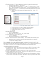
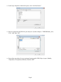
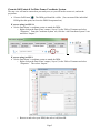
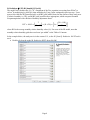
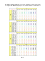
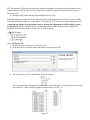
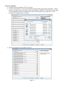
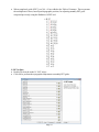
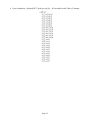
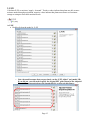
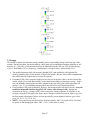
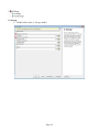
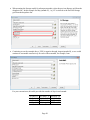
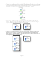
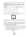
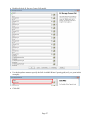
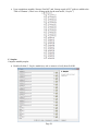
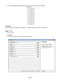
User’s Guide for Water Balance Toolbox (v. 2.2) for ArcGIS
(last modified March 2015)
James Dyer
Department of Geography
Ohio University
A Water Balance Primer
All organisms require energy and moisture, and these two factors have an interactive influence. A water
balance (or budget) explores the relationship between energy and moisture at a place, by modeling
moisture demand (potential evapotranspiration) and supply (precipitation and soil moisture storage). If all
soil pores are filled with water, the soil is saturated. Gravitational water drains away, leaving a film of
capillary water, and the soil is at field capacity. This is the Available Water Capacity (AWC), and is the
water used by plants. If this water is used up so that only hygroscopic water remains, the permanent
wilting point has been reached.
Glossary of terms:
 Potential evapotranspiration (PET, PE, POTET, Et) is the evaporative water loss from a vegetated
surface in which water is not a limiting factor; it depends mainly on heat and radiation.
 Actual evapotranspiration refers to water loss from a vegetated surface given water availability,
and is equal to available water or potential evapotranspiration, whichever is less.
 Deficit refers to evaporative demand not met by available water, or the difference between
potential and actual evapotranspiration.
 Surplus is excess water not evaporated or transpired, that leaves a site through runoff or
subsurface flow.
 Available Water Capacity (AWC) is the maximum amount of water that the soil can store,
representing the soil’s “field capacity.”
Before You Start: Important Information
For ease of use, the model executes with default filenames and file locations. The downloaded zipped
folder containing the Water Balance Toolbox includes a nested series of “blank” folders, named “WB.”
For ease of use, you should unzip this folder to your computer’s C:\ drive (i.e., C:\WB\). If not, many
“automatic” grid names will have to be changed in each of the Toolbox’s models (increasing execution
time, and the likelihood of making an error).
Nested within the WB folder is a folder called “_New_to_Copy.” After you run the complete water
balance model, you can copy the entire C:\WB folder to a new location (you may wish to give it a new
name, e.g., WB-Study_Area_Name), and re-create an empty C:\WB\ folder to run a new model – simply
copy the contents of “_New_to_Copy” to the new C:\WB\ folder.
What you will need for your study area before you start:
 A digital elevation model (DEM). (X, Y units should be the same as elevation (Z) units.)
o Use ArcCatalog to copy the DEM to the C:\WB\DEM\ folder
o When the Water Balance Toolbox is started in ArcGIS, this grid will be named DEM in the
Table of Contents
o A recommended (but optional) tool requires slope and aspect grids (named Slope and
Aspect in the Table of Contents); after creating these grids from your DEM in ArcGIS,
copy them to the C:\WB\DEM\ folder
Page 1




Monthly temperature (°C) and precipitation (mm) grids, and an annual precipitation grid.
o Copy these climate grids to C:\WB\Climate\
o The monthly grids will be named temp-c_01 - temp-c_12, and precip-mm_01 - precipmm_12 when running the Water Balance model. The annual precipitation grid will be
designated precip-mm_13. If you do not have an annual precipitation grid, follow these
steps to create one:
 Double-click on Cell Statistics tool (Spatial Analyst Tools – Local – Cell
Statistics):
 Use the dropdown to select the 12 monthly precipitation grids.
 For the output raster, enter C:\WB\Climate\precip-mm_13
 For the Overlay statistic, select SUM
 Click OK.
Monthly radiation grids
o Copy to C:\WB\Radiation\
o These grids will be named rad_01 - rad_12 in the model.
A soil available water capacity (AWC) grid
o Copy to C:\WB\Soils\
o This grid will be named soil_awc_mm in the model.
Optional, for arid environments (relative humidity < 50%): Monthly relative humidity grids
o No default location is specified in the model; these grids could also be copied to
C:\WB\Climate\ using ArcCatalog.
Refer to Appendix A for a more detailed description, including information about specific data
preparation used for the sample grids in the examples that follow. There is additional information on the
Water Balance Toolbox for ArcGIS web page with information about acquiring these grids.
A word about the grids used in the model
 All input grids (e.g., climate, soil) should be same resolution as DEM. (If necessary, use Data
Management Tools – Raster – Raster Processing – Resample, or Spatial Analyst Tools –
Generalization – Aggregate.)
 All grids are floating point. (Use Spatial Analyst Tools – Math – Float if necessary.)
 All grids should be in the same projection. (If necessary: Data Management Tools – Projections
and Transformations – Raster – Project Raster.)
 Cells for all grids should align. (Subtracting two grids whose cells are misaligned may result in
erroneous values, such that the water balance “final checks” fail; discrepancies should be minor,
Page 2
however.) If you need to align grids, zoom into a single pixel and use the Measure Tool to
determine the amount of x, y shift required. Then use the ArcGIS “Shift” tool to align the grid
(utilizing the tool’s “Input Snap Raster” option: Data Management Tools – Projections and
Transformations – Raster – Shift.).
Using the Water Balance Toolbox in ArcGIS.
(note: the model was created using ArcGIS v. 9.3, but has been successfully executed in ArcGIS v. 10)
Numerous grids will be created upon running the complete Water Balance Toolbox. To aid with
organization, a “Start_Template.mxd” ArcGIS project is provided in the C:\WB\ folder. Open this
project, and you will see that the Table of Contents is “pre-populated” with all the grids that will be
created by the model. Since the grids have not yet been created, a red exclamation point precedes each
name:
Pre-populated Table of Contents visible in “Start_Template.mxd.” Note that the “Water Balance”
toolset is automatically added to the ArcToolbox.
Assigning Names to Existing Grids
If you used the file and naming conventions in the “Before You Start” section, there will be no red
exclamation points adjacent to these grids (DEM, soil AWC, precipitation, etc.). However, if your grids
are named differently, the first step will be to assign names to these existing grids. Below is an example
for assigning a name to the DEM grid.
 Right-click on the red exclamation point adjacent to “DEM” in the Table of Contents and select
“Properties.”
Page 3

In the Layer Properties window that opens, select “Set Data Source:”

Browse to and select the DEM for your study area. (In this example, C:\WB\DEM\dem_scbi).
Click “Add” then “OK.”

Repeat these procedures for any unassigned existing grids: DEM, Slope, Aspect, Monthly
Temperature, Precipitation, Radiation, and Soil AWC.
Page 4
Zoom to Full Extent & Set Data Frame Coordinate System.
The map view will not be centered on your study area, so you will need to zoom to it, and set the
projection.

Zoom to Full Extent
. The DEM grid should be visible. (You can turn off the individual
DEM grid at this point, but leave the DEM Group turned on.)
If you are using ArcGIS 10:
 Set the Data Frame’s coordinate system to match the DEM:
o Right-click on the Data Frame’s name (“Layers”) in the Table of Contents and select
“Properties.” From the Coordinate System tab, click the “Add Coordinate System” icon
and select “Import:”
If you are using ArcGIS 9:
 Set the Data Frame’s coordinate system to match the DEM:
o Right-click on the Data Frame’s name (“Layers”) in the Table of Contents and select
“Properties.” Then select “Import:”
o Browse to and select your DEM, then select Add, then OK.
Page 5
Save the Project
Use File – Save As to rename the “Start_Template.mxd” project to a more meaningful name. (In this
example, C:\WB\WB_SCBI.mxd)
Note: the Water Balance Toolbox utilizes the Spatial Analyst extension. If necessary, turn on the
extension (Tools drop-down menus  Extensions)
Running the Water Balance Toolset
All models in the Water Balance Toolbox can be run by “double-clicking” and entering model parameter
values. Grids will be added to the Table of Contents as each model runs. (Grids are turned off
(unchecked) to reduce redrawing time, but can be turned on for viewing. Note: A Hillshade of your DEM
(Spatial Analyst Tools – Surface – Hillshade), set to 50% transparency and viewed over your Water
Balance grids provides a good “topographic influence” perspective.)
Expand the Water Balance toolbox. We will run the models in
sequence (by double-clicking on the appropriate model name).
1. Turc PE
Calculates monthly Potential Evapotranspiration according to Turc (1961):
𝑃𝐸𝑇 = 0.013 × [
𝑇
] × (𝑅 + 50)
(𝑇 + 15)
where PET is potential evapotranspiration (mm), T is temperature (°C), and R is radiation (Wh/m2)
Page 6
A: Temp Factor
The first tool computes the “temperature” component of the Turc equation above. Since PET is
temperature dependent (if the monthly temperature ≤ zero, then PET = 0), the model first checks for
negative temperatures. The output is used as input for the subsequent PET tool.
 Double-click on the model A: Temp Factor, then click OK.

After the model is executed, the new grids are added to the Table of Contents; red exclamation
points adjacent to the t_factor grid names disappear:
Page 7
B: Radiation  PET (B1 [humid], B2 [arid])
The model first calculates the “R + 50” component of the Turc equation (converting from Wh/m2 to
cal/cm2 by multiplying by 0.08598,) then multiplies by Temp_factor computed in previous step. Users
must select either the B1 [humid] model, or the B2 [arid] model, based on the climate of their study area.
If relative humidity is <50%, model B2 [arid] would be more appropriate, which computes Potential
Evapotranspiration with a Relative Humidity adjustment factor:
𝑃𝐸𝑇 = 0.013 × [
(50 − 𝑅𝐻)
𝑇
] × (𝑅 + 50) × [1 + (
)]
(𝑇 + 15)
70
where RH is the average monthly relative humidity value (%). For users of the B2 model, note that
monthly relative humidity grids have not been “pre-added” to the Table of Contents.
In the example below, the study area is in the eastern U.S., so the B1 [humid]: Radiation  PET tool is
used.
 Double-click on the model B: RadiationPET, then click OK.
Page 8

Upon completion, grids PET_01 – PET_12 are added to the Table of Contents:
1B. PE Adjust
Note: The discussion here focuses on seasonal climates in the northern hemisphere, in which maximum
insolation occurs on southern aspects during the growing season (defined as April-September). Users in
the southern hemisphere, or in climates with a year-round growing season, will need to adjust the
methodology accordingly.
This toolset is optional for completing the water balance analysis, but it attempts to account for
important temperature changes throughout the day. With a monthly time-step, there is no diurnal
variation in temperature, and so maximum PET occurs on southern exposures, since that is where
maximum insolation occurs. (PET is then symmetrical about the N-S axis.) This toolset employs
“adjustment coefficients” that either increase or decrease PET based on topographic position. The first
step in creating PET adjustment coefficients, therefore, is to create a topographic grid based on the
existing slope and aspect grids for the study area.
PET Adjustment Coefficients were computed for 4 sites in the northern hemisphere (eastern U.S.), and
can be used as models for other study areas:
 Williamsport PA (41°N)
 Elkins WV (39°N)
 Beckley WV (37°N)
 Asheville NC (35° N)
These were created using “Typical Meteorological Year” data published by the National Solar Radiation
Database. In the tables below, the amount of increase (>1) or decrease (<1) to PET values based on
topographic position can be observed for each of these sites:
Page 9
PET adjustment coefficients for the entire growing season, standardized so that flat sites (0-1° slope)
have a value of 1.000. Multiplying PET values by these coefficients increases (>1) or decreases (<1)
moisture demand based on topographic position.
Page 10
PET Adjustment Coefficients have also been computed for another site using recorded temperature and
radiation data for 2003 & 2010; the PET Adjustment Coefficients for this site represent the average of
these two years:
 McArthur OH [Vinton Furnace Experimental Forest] (39°N)
Monthly adjustment coefficients for the growing season (April-September) for all five sites are available
in the Water Balance toolbox as “remap tables” (used in the B: PET Coefficients model described below).
A detailed description of the procedures used to develop the Adjustment Coefficient grids is given
in Appendix B, and an ArcGIS model for creating adjustment coefficient grids is also available for
download from the Water Balance Toolbox for ArcGIS web page.
A: Create Topo Grid
 Double-click on the model A: Create Topo Grid
 In the drop-down, select the Slope and Aspect Grids, then click OK.

The grid “slop9_asp12” is added to the Table of Contents:
The 93 classes in the grid represent combinations of slope and aspect. For example, an east-facing
pixel with a 22° slope would be assigned a reclass value of 45 (40 + 5).
Page 11
B: PET Coefficients
 Double-click on the model B: PET Coefficients
 Specify a Remap table (*.rmp) for each month in the growing season (April-September). Unless
you have computed your own values, browse to the folder C:\WB\PET_Coeffs and select the table
for the appropriate month, selecting the site closest to the latitude of your study area. In the
example, 39°N (Elkins WV) is selected:

When each month has been added, click OK:
Page 12

When completed, grids of PET_coef_04 – 09 are added to the Table of Contents. These represent
the multiplicative factor, based upon topographic position, for adjusting monthly PET grids
computed previously using the Radiation  PET tool.
C: PET Adjust
 Double-click on the model C: PET Adjust
 Click OK to perform the topographic adjustment to monthly PET grids:
Page 13

Upon completion, “Adjusted PET” grids (pet_adj_04 – 09) are added to the Table of Contents:
Page 14
2. P-PE
Calculates P-PE, or moisture “supply – demand.” Positive values indicate that plants are able to meet
moisture needs through precipitation, negative values indicate that plants must turn to soil moisture
storage to attempt to meet their moisture needs.
A: P-PE
 Double-click on the model A: P-PE
o Note: the model assumes that you previously ran the “PET Adjust” tool (model 1B).
If you did not, you will need to specify the original PET grids instead of the Adjusted
Potential Evapotranspiration grids (months 04-09), as shown in this figure:
Page 15

Click OK. Several grids are added to the Table of Contents: Annual PET, Monthly P-PE, and
Daily P-PE (necessary for the subsequent Storage tool). (Your P-PE values will be different than
in the example below):
Page 16
3. Storage
This model computes soil moisture storage (monthly values, representing storage on the last day of the
month). During execution, the model employs a daily time step, assuming decreasing availability of soil
moisture (i.e., only 50% of soil moisture need can be obtained when the soil is at 50% of field capacity;
Curve C from Mather 1974, Climatology: Fundamentals and Applications. McGraw-Hill, NY).




The model determines daily soil moisture demand (P-PE) and availability (Precipitation) by
dividing monthly values by the number of days in the month. Because it does daily computations,
this model takes the longest time to execute; be patient!
If monthly P-PE values computed in the previous step are all positive, there is no need to run this
model: supply (P) exceeds demand (PE), so the plants do not utilize soil moisture storage. In this
case, the monthly Storage grids can all be assigned as the Soil AWC grid (which represents full
storage). See “To set remaining storage grids to the Soil AWC grid” instructions below.
If any monthly P-PE grids are negative, however, the Storage model will need to be run. Start the
model for the month with first negative P-PE values, when Storage is full. Storage can
assumed to be full (i.e., Storage=AWC) after consecutive months of positive P-PE grids. As an
example, using the P-PE grids in the figure above, Storage would be first run for April: p-pe_04 is
the first month with negative values, and was preceded by seven months of positive p-pe values
(p-pe_09, 10, 11, 12, 01, 02, 03).
NOTE – Since the Storage model involves dividing a grid by AWC, the result will be “No Data”
for pixels on the Storage grid where AWC = 0 (i.e., where there is water)
Page 17
A: Storage
 Double-click on the A: Storage model:
Page 18

Using the example above, the Storage model will first be run for April, since p-pe_04 was the
first monthly grid with negative values:

Enter the number of days in the month (30 for April), and the “month number” (“04” in this
example) for the P-PE, Daily P-PE, and current month Storage grids.
Since this is the first execution of the model, there is no “Previous Storage” grid. But we are
assuming that Storage is full at the start of April. For this “starting month,” therefore, select
the Soil AWC grid (soil_awc_mm) from the dropdown list.
When the model executes, the first monthly Storage grid is added to the Table of Contents
(st_04 in this example):


Page 19

When running the Storage model for subsequent months, select the previous Storage grid from the
dropdown list. In this example for May (month 05), “st_04” is selected as the Previous Storage
grid from the dropdown list:

Continuing to use the example above, P-PE is negative through August (month 08), so we would
continue to run model consecutively for each of these months, for example, June:
For your convenience, this table provides the number of days in each month:
01 (Jan): 31
02 (Feb): 28
03 (Mar): 31
04 (Apr): 30
05 (May): 31
06 (Jun): 30
07 (Jul): 31
08 (Aug): 31
Page 20
09 (Sep): 30
10 (Oct): 31
11 (Nov): 30
12 (Dec): 31

Continue to run the Storage model after monthly P-PE grids become all positive, since soil storage
has to be recharged. For instance, in our example, September P-PE (p-pe_09) is positive, but soil
moisture has been utilized in each of the previous five months (April – August):

In our example, the Storage model was run for September, and st_09 added to the Table of
Contents. Comparing it to the Soil AWC grid (“full storage”), we can see that more recharge is
required; soil storage is still not up to field capacity for all cells:

Continue to run the Storage model for each month. In our example, the Storage model was run
again for October (month 10). st_10 had values less than the Soil AWC grid, so the Storage
model was run for November (month 11). The values for st_11 are the same as for Soil AWC, so
soil storage may be full (i.e., at field capacity):
Page 21

To be sure that the storage grid is identical to the Soil AWC grid, subtract the storage grid (st_11
in our example) from the AWC grid (Spatial Analyst Tools  Math  Minus) [saved to the
C:\WB\working\ folder]

The result is zero for all cells, indicating that storage is at field capacity:

If the resulting grid contained non-zero (positive) values, the Storage model would need to be run
again for the next month. (The “minus grid” can be removed from the Table of Contents after
viewing.)
When Storage is full, you can continue to run the Storage model. It is time-consuming to execute,
however, so it will save time to assign the remaining storage grids the same values as the Soil
AWC grid. Be sure, however, that a subsequent month’s P-PE grid does not assume negative
values (i.e., P-PE values are negative one month, then positive, then negative again) – the Storage
model must be run for any month with negative P-PE values.
To set remaining storage grids to the Soil AWC grid:
o In this example, st_11 is full, and P-PE is positive for December – March (months 12-03).
Positive P-PE means that plants are not drawing upon soil moisture, so Storage will remain
full for each of those months. Therefore, rather than continuing to run the Storage module,
you can “Set Data Source” for those storage grids, setting them to the values of the soil
AWC grid (which represents full storage).
o Right-click on the red exclamation point adjacent to the Storage grid (in this example,
st_12) in the Table of Contents and select “Properties.”


Page 22

In the Layer Properties window that opens, select “Set Data Source:”

Browse to and select the soil AWC grid for your study area. (In this example,
C:\WB\Soils\soil_awc_mm). Click “Add” then “OK.”


Repeat these procedures for the other “full” storage grids.
Save the project.
Page 23
B. Delta Storage
Computes the difference in Storage from one month to the next; this represents either plant utilization,
or recharge.

Double-click the B: Delta Storage model, then click OK.

The Delta-Storage grids are added to the Table of Contents upon completion:
Page 24
4. AET
Computes actual evapotranspiration, deficit, and surplus.

Double-click the A: AET model (may take a moment to load), then click OK.
Page 25

Upon completion, AET and Deficit grids are added to the Table of Contents:
o Note: Some Deficit grids may contain very small negative values (< -0.001). Although
negative values make no sense conceptually, they are small enough to be ignored.
Alternatively, an “if-then” statement can be added to the model, setting negative values to
zero.
B. Storage Comes Full
This model looks for the month(s) in which the Storage of individual cells comes full. (Soil Storage must
first reach field capacity before there can be Surplus water.) Presumably plants have been utilizing soil
moisture as the growing season progresses; the soil moisture is then recharged (usually) through the fall
and winter.
Page 26

Double-click the B: Storage Comes Full model.

Use the dropdown menu to specify the Soil Available Water Capacity grid (soil_awc_mm in this
example):

Click OK
Page 27

Upon completion, monthly “Storage First Full” and “Storage equals AWC” grids are added to the
Table of Contents. (These serve as input grids for the next model, “Surplus.”)
C. Surplus
Computes monthly surplus.

Double-click the C: Surplus model (may take a moment to load), then click OK.
Page 28

Upon completion, monthly Surplus grids are added to the Table of Contents.
5. Checks
Verifies that the water budget is in “balance,” and that there are no errors in computation.
A. Checks
 Double-click the A: Checks model, then click OK.
Page 29

Upon completion, two “Checks” grids are added to the Table of Contents:

These represent the following checks (the “i” indicates that they are integer grids):
PET = AET + Deficit
Precipitation = AET + Surplus
Resulting annual grids should have all zero values if checks hold. If this is not the case, see the
“troubleshooting” section below.
Troubleshooting (“check” grids not composed of all zeros):
By following all of the naming conventions, potential errors should be minimized. If the checks do not
hold, however, refer to the following for troubleshooting ideas.
 First, consider the magnitude of the errors, keeping in mind that the units are millimeters of water.
If for instance, annual precipitation is 1000 mm, and the maximum error in your “Checks” grids is
2 mm, this represents a 0.2% error, which you may consider negligible.
o Very small errors may be due to grids misaligning. For example, cells of your climate grid
may not align exactly with your radiation grid (derived from the DEM). The result could
be that the “P-PE” procedure subtracts the value of the pixel adjacent to the target cell,
resulting in small discrepancies. See the section “A word about the grids used in the
model.”
 If one of the Check grids is all zeros, and the other is not, this indicates in what steps the error may
have occurred. For example, if one Check grid contains all zeros but the other does not, then the
AET calculations cannot be the problem, since these grids “worked” with the one check. (AET
occurs in both checks.)
 Zoom into non-zero areas. See if a discernible pattern is evident that matches any of your input
grids (e.g., Soil AWC) – this could indicate the problem.
 Use your Identify tool to click on a single cell in the “problem” area, and ascertain the values of all
input grids. See if you can determine where the error has arisen. An Excel spreadsheet that
computes the water balance is available on the Water Balance Toolbox for ArcGIS web page,
which may help in diagnosing individual cells.
Clean Up / File Maintenance
You will likely want to save your original input grids (Temperature, Precipitation, Radiation, Soil
Available Water Capacity, DEM), as well as the “key” water balance grids (PET, Storage, AET, Deficit,
and Surplus). However, many of the grids created with the Water Balance tool are “intermediate,” only
necessary as input for various models. These can be deleted to save disk space (once you are sure your
checks hold from Step 5!). Save and close your ArcGIS project, then you can delete the following folders
in C:\WB\: Checks, subfolder “Temp_Factors” (in Climate folder), P-PE. If you are not interested in soil
moisture storage grids, you can delete the entire Storage folder. Otherwise, use ArcCatalog to delete all
of the grids except ST_## grids in the Storage folder. If you open your saved Water Balance .mxd project
after performing the deletions, a red exclamation point will appear next to the deleted grid names. You
can remove these from the Table of Contents and re-save the project.
Page 30
APPENDICES
A: Notes on Data Preparation and Grid Creation used in this User Manual
B: Procedure used for computing PET adjustment coefficients
C: Input/Output grids used in the Water Balance toolbox
D: Conceptual steps in computing a water balance
Page 31
Appendix A:
Notes on Data Preparation and Grid Creation used in this User Manual
In the examples used in this user manual, all grids are in the same projection (using: Data Management
Tools – Projections and Transformations – Raster – Project Raster as necessary). Specifically, the DEM
and all grids are in UTM; with this projection, “x,y” units (meters) are the same as the “z” (elevation)
units, which is another requirement for DEMs in the model.
1. The Digital Elevation Model was downloaded from the USGS National Map Viewer (selecting
the finest resolution available)
2. In ArcGIS, a rectangular shapefile of the study area was created, so that input grids (including the
DEM) can be clipped to a common extent (Data Management Tools – Raster – Raster Processing
– Clip).
3. Soil Data (Available Water Capacity) can be downloaded from the USDA-NRCS “Web Soil
Survey” web page. Step-by-step instructions:
a. Start Web Soil Survey
b. Define Area of Interest. (The study area shapefile created in Step 2 can be uploaded to
define your Area of Interest.)
c. Click on the “Download Soils Data” button along the top of the screen.
d. Preparing the grid for use in the Water Balance toolbox:
 After downloading and unzipping the soil data from the Web Soil Survey, double-click
on the soil data “.mdb” file to open it in Microsoft Access 2010.
 If prompted, “Stop all Macros,” and “Enable Content.”
 Exit out of the Soil Reports window that appears.
 In the left navigation panel, select Tables. Double-click on muaggatt (“map unit
aggregated attribute table”) to view it.
 Click on the “External data” tab at the top of the screen, and select the “Export to Excel
spreadsheet” icon.
o In the “File format” window, select “Excel 97 – Excel 2003 Workbook (*.xls)”
o Do not check “Export data with formatting and layout.”
 Open the new file in Excel.
 You will need to retain columns “mukey” and “aws0100wta” (“Available Water
Storage 0-100 cm – Weighted Average” – although other depths are available if
preferred).
 Since the “aws” value is in cm, create a new column (“AWC_mm”) multiplying aws ×
10. (Note: Water polygons have a “No Data” value for AWC.)
 Save the Excel file (keeping the *.xls format). Close it. You can now add this Excel
file to ArcGIS, and join it to the “soilmu_a” shapefile found in the downloaded
“spatial” folder.
Page 32

Convert this “joined” polygon shapefile to a grid:
o ArcToolbox – Conversion Tools – To Raster – Polygon to Raster:
o Input = soils shapefile
o Value field = AWC_mm
o Output = soil_AWC_mm
o Cell Assignment Type = MAXIMUM_COMBINED_AREA
o Cellsize = same cellsize as the DEM you will use for the water balance analysis
(you can browse to the DEM and select it)
4. Obtain monthly temperature and precipitation data.
a. In the current example, I obtained 1981-2010 climatic normals from NOAA’s National
Climatic Data Center. Data need to be properly formatted, and converted to °C and mm.
Annual values should also be computed.
i. Monthly climate grids can be created by multiplying the DEM by zero (Spatial
Analyst Tools – Math – Times) for each necessary monthly grid (25: monthly
temperature and precipitation, annual precipitation).
ii. Then add the appropriate climate value to the “zero grid” to create individual
temperature or precipitation grids (Spatial Analyst Tools – Math – Plus).
b. As another alternative, gridded climatic data for the US is also available from PRISM.
(ModelBuilder may be useful to automate these repetitive steps.)
i. You will need to clip the monthly climate grids to your study area (Analysis Tools –
Extract – Clip). It may be advisable to buffer your study area to create a larger clip
to insure complete coverage at the end of the processing steps (Analysis Tools –
Proximity – Buffer).
ii. PRISM grids are integer, with units x 100. Therefore:
1. The integer PRISM grids will need to be converted to floating point (Spatial
Analyst Tools – Math – Float).
2. The resultant grids will then need to be divided by 100 (Spatial Analyst
Tools – Math – Divide).
iii. The relatively coarse resolution climate grids can then be set to the resolution of
your DEM (Data Management Tools – Raster – Raster Processing – Resample).
iv. This final, fine-resolution climate grid can be clipped to your actual study area
boundary (as opposed to a buffered study area).
Page 33
Appendix B:
Procedure used for computing PET adjustment coefficients
 Hourly solar radiation was computed for 2 days each month (two-week intervals) from AprilSeptember, using the ArcGIS Solar Radiation toolset
 PET was then computed for each day, using hourly temperature, as well as a single average daily
temperature value for each hour. Hourly temperature data were from “Typical Meteorological
Year [TMY3]” data: http://rredc.nrel.gov/solar/old_data/nsrdb/1991-2005/tmy3/.
 Daily PET was summed for the two days to create a representative monthly value.
 The ratio of average/hourly-temperature PET was standardized so that flat sites (0-1° slopes) = 1.
(Flat sites should be unaffected by diurnal variations in radiation/temperature.)
 Note that the topographic adjustment factors vary monthly, vary with latitude, and are not
symmetrical about a particular compass axis.
Instructions for creating your own PET adjustment coefficients, including an ArcGIS model, are available
for download from the Water Balance Toolbox for ArcGIS web page.
Page 34
Appendix C:
Input/Output grids used in the Water Balance toolbox
1. Turc PE
A. Temp_Factor
Input
 Average monthly temperature (°C)
o example: Climate\Temp\temp-c_01
Output
 Monthly temperature factors (t_factor_##)
o example: C:\WB\Climate\Temp_Factors\t_factor_01
B. Radiation-->PET
Inputs
 Monthly temperature factors (from above)
o example: Climate\Temp Factors\t_factor_01
 Monthly radiation from Solar Analyst (WH/m2)
o example: Radiation\rad_01
 Monthly relative humidity (%) – optional, used with the B2 [arid] model.
Output
 Monthly PET (PET_##) in mm
o example: C:\WB\PET\PET_01
1B. PE Adjust
A. Create Topo Grid
Input
 Slope grid (°)
 Aspect grid (°)
Output
 Reclassed slope and aspect grid
o C:\WB\DEM\slop9_asp12
B. PET Coefficients
Inputs
 Reclassed slope and aspect grid (from above)
o DEM\slop9_asp12
 Remap tables with PET Adjustment Coefficients (growing season, months 04-09)
o example: C:\WB\PET_Coeffs\PET_Adj_41N_04.rmp
Output
 Monthly PET Coefficients (growing season, months 04-09)
o example: C:\WB\PET\PET_coef_04
C. PET Adjust
Inputs
 Monthly PET grids (PET_##) (growing season, months 04-09)
o example: PET\pet_04
 Monthly PET Coefficients (from above)
o example: PET\PET_coef_04
Output
 Monthly Adjusted PET (mm) (growing season, months 04-09)
o example: C:\WB\PET\pet_adj_04
Page 35
2. P-PE
A. P-PE
Inputs
 Average monthly precipitation (mm)
o example: Climate\Precip\precip-mm_01
 Monthly PET grids (PET_##), or Adjusted PET grids (pet_adj_##)
o example: PET\PET_01, or PET\pet_adj_04
Output
 Monthly P-PE grids (P-PE_##), in mm
o example: C:\WB\P-PE\P-PE_01
 Daily P-PE grids (Daily_P-PE_##), in mm
o example: C:\WB\P-PE\Daily_P-PE_01
 Annual PET (mm)
o example: C:\WB\PET\pet_annual
3. Storage
A. Storage
Inputs
 Number of days in the current month.
01 (Jan): 31 05 (May): 31 09 (Sep): 30
02 (Feb): 28 06 (Jun): 30 10 (Oct): 31
03 (Mar): 31 07 (Jul): 31
11 (Nov): 30
04 (Apr): 30 08 (Aug): 31 12 (Dec): 31
 Soil AWC grid (Soil\soil_awc_mm)
 P-PE grid (P-PE\p-pe_##) for current month (mm)
 Daily P-PE grid (P-PE\Daily_p-pe_##) for current month (mm)
 Storage for the previous month (ST_##), in mm.
 NOTE – for first month run (i.e., the month where Storage come full), use the AWC
grid (Soil\soil_awc_mm) for previous month Storage, ST_## (since full storage =
AWC).
Output
 Storage for the current month (ST_##), in mm
o example: C:\WB\Storage\ST_04
B. Delta Storage
Inputs
 Storage for each month (e.g. Storage\st_04), mm
Output
 Delta Storage (Difference in Storage) for each month, in mm
o example: C:\WB\Storage\delta_ST_05
4. AET
A. AET
Inputs
 Average monthly precipitation (Climate\Precip\precip-mm_##), mm
 Potential evapotranspiration (PET\PET_##) or Adjusted PET (PET\adj_pet_##), mm
 P-PE grids (P-PE\p-pe_##), mm
 Delta Storage grids (Delta_ST\delta_ST_##), mm
Page 36
Outputs
 Monthly actual evapotranspiration (mm)
o C:\WB\AET\AET_##
 Monthly deficit (mm)
o C:\WB\Deficit\Def_##
 Annual actual evapotranspiration (mm)
o C:\WB\AET\AET_Annual
 Annual deficit (mm)
o C:\WB\Deficit\Def_Annual
B. Storage Comes Full
Inputs
 Soil AWC grid (Soil\soil_awc_mm)
 Storage for each month (e.g., Storage\st_08), mm
Output
 Storage-first-full grid for each month; values 1 (first full) or 0
o example: C:\WB\Storage\st1stfull_09
 Storage = AWC grids (1=yes, 0=no)
o example: C:\WB\Storage\ST_eq_AWC_09
C. Surplus
Inputs
 Average monthly precipitation (Climate\Precip\precip-mm_##), mm
 Monthly actual evapotranspiration (AET\aet_##), mm
 Storage = AWC grids (ST_1st_Full\ST_eq_AWC_##), 1/0
 Delta Storage grid (Delta_ST\delta_ST_##), mm
 Storage-first-full grid (ST_1st_Full \ST1stFull_##), 1/0
Output
 Monthly Surplus (mm)
o C:\WB\Surplus\Surplus_##
 Annual Surplus (mm)
o C:\WB\Surplus\Surplus_Ann
5. Checks
A. Checks
Inputs
 Annual precipitation (Climate\Precip\precip-mm_13), mm
 Annual Potential Evapotranspiration (PET\PET_Annual), mm
 Annual Actual Evapotranspiration (AET\AET_Annual), mm
 Annual Deficit (Deficit\Def_Annual), mm
 Annual Surplus (Surplus\Surplus_Ann), mm
Output
 P=AE+Surplus “check grid” (all zeros if checks hold)
o C:\WB\Checks\p_ae_s_i
 PE=AE+Deficit “check grid” (all zeros if checks hold)
o C:\WB\Checks\pe_ae_def_i
Page 37
Appendix D:
Conceptual steps in computing a water balance
You will need P (precipitation, “supply”) and PE (potential evapotranspiration, “demand”) to start.
A. P-PE  tells when demand exceeds supply (P-PE will be negative).
 If supply (P) < demand (PE), plants utilize soil water.
 If supply (P) > demand (PE), there is more water than plants need.
 Available water is prioritized as follows:
1. Plants use what they want (first from precipitation, then from soil storage)
2. If there is still water leftover, it is used to recharge storage if it is not full
3. Any excess water becomes surplus
B. Determine where soil water storage (ST) will be full [= AWC], based on consecutive values of PPE.
C.  ST = change in ST from month to month (water used by plants or to recharge storage).
D. AE – what plants use. If water is not limiting, plants take what they want (AE=PE).
 Whenever ST =AWC, AE = PE (water is coming from P)
 As ST is depleted, it becomes increasingly difficult for plants to extract the water they need.
 When ST < AWC, AE = P +  ST (AE may be less than PE. It can never be more)
E. Deficit: PE - AE. By how much plants “came up short.”
F. Surplus. If ST is full (=AWC), there’s liable to be “excess precipitation” – plants don’t use it all.
 If ST < AWC, there can be no Surplus.
 If ST = AWC, then S = P - AE.
 Note the month when ST reaches AWC, S = P - AE -  ST (excess first went to fill Storage).
G. Checks on annual totals:
 PE = AE + D
 P = AE + S
Page 38