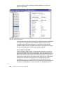
Download Planning and Implementing an IBM SAN - ps

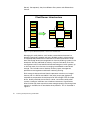
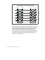
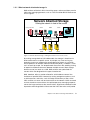
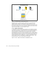
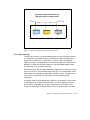
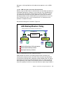
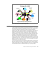
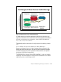
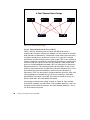
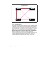
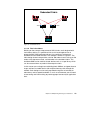
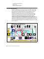
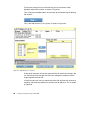
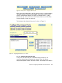
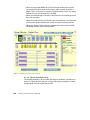
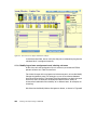
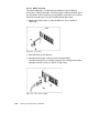
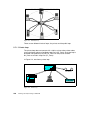
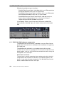
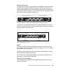
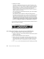
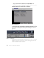
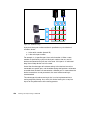
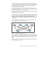
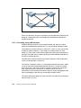
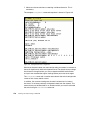
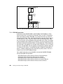
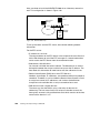
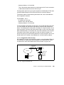
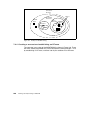
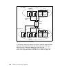
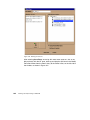
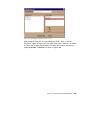
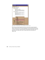
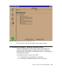
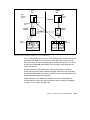
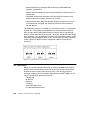
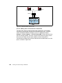
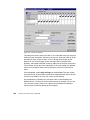
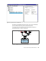
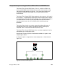
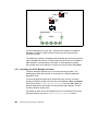
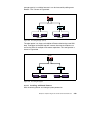
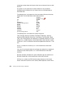
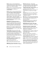
7.5.1 Multiswitch fabric considerations
The planning of multiswitch fabrics depends on many things. Are you going to
have a local SAN in one site with up to 32 devices connected? Then you may
not want to consider cascading switches. If you want to build a SAN between
two sites that are far apart, cascading becomes valued. Also, if you need
more devices connected, or if you are looking to introduce extra redundancy,
cascading is the only way to achieve this.
Nevertheless, we still might think about whether or not, or to what extent, we
want to cascade switches. The reason for this is that by using E_Ports we will
sacrifice F_Ports. Also, with an extended fabric, the ISLs can possibly
become a bottleneck. This will lead to the use of more ISLs, which means
even fewer F_Ports.
What seems easy in the first instance, can get more complicated once we
add the zoning concept, load balancing, and any bandwidth issues that may
appear.
7.5.1.1 Where multiswitch fabrics are appropriate
Certainly, there are some possible solutions where a multiswitch fabric is
needed. For example, disaster recovery solutions that are using a SAN can
be built upon a McDATA SAN, but only when using E_Ports to connect
directors between two sites. We need directors at both sites to back up one
site completely. Disaster recovery and high availability can be established
together using a multiswitch fabric, and open system hosts using Logical
Volume Manager (LVM) mirroring together with clustering software, such as
HACMP for AIX or Veritas Cluster Server. Due to the high availability and the
many ports of the McDATA ED-5000, two McDATA ED-5000 may be enough.
7.5.1.2 Solutions for high availability and disaster recovery
An example of a solution that provides high availability with disaster recovery,
is shown in Figure 200.
238
Planning and Implementing an IBM SAN