1
Prof. R.J. Jones
Optical Sciences
OPTI 511L
Fall 2014
(Part 1 of 2)
Experiment 1: The HeNe Laser, Gaussian beams, and optical cavities
(~3 weeks total)
In these experiments we explore the characteristics of the transverse and longitudinal modes of
two-mirror optical resonators and Helium-Neon lasers, as well as the higher-order HermiteGaussian modes of a Helium-Neon laser. We also explore the possibility of generating other
beam-like solutions to the wave equation, namely Laguerre-Gaussian beams.
The appendix at the end contains several useful equations for this lab.
Overview of specific objectives:
(Part 1)
(i)
Explore the concepts of resonance, spatial mode-matching, and resonator stability using the
TEM00 transverse mode of a Helium-Neon laser and an external two-mirror optical cavity.
(ii)
Learn to use a scanning confocal Fabry-Perot interferometer (FPI) for optical spectrum
analysis and why such a cavity configuration is often used.
(Part 2)
(iii) Learn to align and operate an open-cavity Helium Neon laser and explore conditions for
resonator stability and fundamental-transverse mode operation.
(iv) Generate higher-order Hermite-Gaussian modes, and determine the optical frequency
spectrum associated with the different transverse modes of a spherical mirror cavity.
(v)
Generate beams other than the Hermite-Gaussian modes by converting Hermite-Gaussian
beams to Laguerre-Gaussian beams with a cylindrical telescope.
Gaussian Beams and Optical Cavities, Fall 2014.
1
(i) Modes of an optical resonator
One of the most basic and common methods used in the characterization of laser light involves
sending laser light into an external optical cavity. Because laser light properties such as optical
frequency and transverse spatial modes are dependent on the optical resonator that is part of the
laser, we can think of the laser light as carrying information about the laser resonator. By
sending the laser light into a separate (passive) optical cavity, the laser light can be analyzed as
long as we know the characteristics of this second external cavity. In a sense, by sending laser
light into an external resonator, we are using one optical cavity to characterize another.
To understand better how this process works, in the first part of this lab you will send a beam of
laser light into an external cavity that you will construct. Because the external cavity length
changes randomly due to mirror vibrations and pressure fluctuations, the injected laser light will
be resonantly coupled to different cavity modes (longitudinal and transverse) at different points
in time. Remember that resonant coupling will only occur when at least one of the frequency
components of the laser light matches at least one of the mode frequencies of the external cavity
(which are changing in time due to mirror vibrations, etc.). Since resonant coupling of light into
an external cavity also leads to enhanced transmission of the light through the external cavity,
you will be able to see the effects of the time-dependent coupling by looking at the changes in
the intensity profile of the beam as it exits the external cavity.
Suppose the laser light is purely monochromatic, and has a TEM00 beam profile. The ideal
situation for transmitting the laser light through an external cavity would be to have the external
cavity length stabilized (fixed), with the frequency of the laser light resonant with the frequency
of one of the modes of the cavity. Furthermore, the spatial profile of the incident laser beam
would ideally be matched to a transverse mode of the passive optical cavity: if the laser light
propagates in a TEM00 mode (by which we mean the fundamental transverse mode of the laser
resonator), we would ideally want it to match the fundamental transverse mode (TEM00) of the
external cavity. Such mode matching does not occur automatically, since the fundamental
external cavity mode will have its own set of Gaussian parameters of spatially varying beam
width and radius of curvature, entirely independent of the parameters of the laser resonator. To
mode-match the laser TEM00 mode to that of the external cavity mode, lenses must usually be
used to shape the incoming beam so that the parameters of the incident laser beam match those
of the cavity.
As usual, the experimental situation is more complex than the ideal case. If the laser beam is not
perfectly aligned and mode-matched to the external cavity, the input beam will partially couple
to many different transverse modes of the optical cavity (the mode of the input beam can be
described as a superposition of external cavity eigenmodes- such as the Hermite-Gaussian
modes), and the light that exits the cavity will resemble whatever cavity modes happen to be
excited rather than maintaining the spatial profile of the input beam. Since we will not stabilize
the length of the cavity, the coupling of the laser beam to the longitudinal and transverse cavity
modes will change with time, and the light patterns that are observed exiting the cavity will
fluctuate with time, resulting in a time-dependent (fluctuating) coupling of the laser beam to
many different high-order Hermite-Gaussian modes of the optical cavity.
Gaussian Beams and Optical Cavities, Fall 2014.
2
In this lab you will be using a few different HeNe lasers of various length. The first HeNe laser
will be set up for you when you begin the lab. The output coupler of this HeNe has a flat mirror.
Your first task in this lab is to determine the laser beam waist exiting the laser. To get an
estimate for this, measure the beam divergence several meters away from the laser (in the “farfield”). You can estimate this by just using a piece of paper to mark the approximate beam
diameter at a few locations spaced by several meters. In the far-field, the beam will expand
linearly. By measuring this far-field angle, you can estimate the initial beam size using the
Gaussian beam propagation expressions and making reasonable approximations (i.e. the distance
“z” is much greater than the Rayleigh range). EXTRA CREDIT if you can tell me the radius of
curvature of the second HeNe cavity mirror. Please make a sketch of the laser cavity, the
exiting laser beam diameter from your measurements, and your calculation for the beam
waist.
Your second task in this lab is to attempt to mode-match the TEM00 beam from this HeliumNeon (HeNe) laser to a passive optical cavity which you will construct using two mirrors (M1
with ROC = 120 cm and M2 with ROC=120cm). The layout is shown in Figure 1. You do not
need to perfectly mode-match to the cavity, but you should get a feel for what the requirements
are and the challenges associated with mode-matching are.
For this 2-mirror cavity, where will the beam waist be located? Please sketch the cavity and
answer this question in your lab book.
Steps for the mode-matching section:
1. Set up the laser so that the beam is at a convenient height above the table, and is parallel to
the table. Use a mounted iris or other height marker to make sure the beam is parallel to the
table.
2. Use two mirrors as folding mirrors, as shown in the figure. These mirrors can help in
aligning the beam with the external cavity (first align the external cavity as best you can, then
use these 2 mirrors to make fine adjustments). In setting up the mirrors, make sure the beam
stays parallel to the table. Further alignments will be made more convenient if, after
bouncing off of the second mirror, the beam propagates (approximately) over a row of holes
in the optical table. Again, use a mounted iris to help with this alignment.
HeNe laser
mirror
screen
M2
M1
mirror
Lens 1
Lens 2
L
Fig. 1. Schematic of 2 mirror optical cavity. Make sure to focus the beam in such a way to
form a waist at the correct position of the external 2-mirror cavity.
Gaussian Beams and Optical Cavities, Fall 2014.
3
3. Set up the iris that you have been using at the edge of the table, over a bolt hole. The beam
should hit the iris center. Make sure that there is plenty of room on the table along the beam
path after the focus of the beam. Use the iris as an alignment tool for centering the lens, and
use a sheet of lens paper as a quick tool to find the position of the beam focus. An optical rail
can be used to translate lens 1 and allow fine adjustment for the position of the beam waist.
4. To optimally mode-match to the external cavity, the position and size of the beam waist
generated by lens 1 must match that of the beam waist defined by the external cavity mirrors
M1 and M2. To begin with, let’s focus on getting the beam waist in the right location, and
worry about the size of the beam later. You will find that if the beam waist is at the correct
location, the cavity will be fairly close to mode-matched. Getting both the beam waist
position and size correct is more challenging.
To begin, use the f=50 cm lens that is available to focus the HeNe beam and form a beam
waist where the waist of your 2-mirror cavity will be located.
5. Choose what length you will use for your 2 mirror cavity and calculate what the beam waist
for the cavity will be. Make sure you choose a length that satisfies the stability criterion.
6. Now you will align the 2-mirror optical cavity. First set up the M2 so that the beam hits the
mirror near its center, and so that the beam is directly retro-reflected. Be sure to position the
mirror correctly for the length you chose in step 5. The coated mirror surface should face into
the cavity that you are building. How does this single mirror affect the spatial
characteristics of the low-power beam that is transmitted through the mirror?
7. Install the second mirror M1 so that the coated surface of M1 is facing M2. For good spatial
mode matching, it is important to get the laser beam waist right at the cavity waist position.
You can optimize this later with the position of lens 1. Also, try to get the beam to hit the
center of M1. Place a card within the external resonator to block the light in the cavity.
There will be a fraction of light that is reflected from M1 back towards the laser, possibly
resulting in multiple spots due to the beam bouncing back and forth between M1 and other
optics (such as the laser's output coupler). Adjust M1 so that these spots overlap the forwardpropagating beam.
8. You should now have a cavity that is close to being aligned. Remove the card from the
cavity and look on the observation screen for the transmitted light. If desired, you can use a
short focal length lens to expand the transmitted beam (lens 2 in the figure) onto an
observation screen directly after M2 (sometimes partially shutting off the lights here helps
too). It often helps to shut off some of the room lights. If the alignment is very close, you
may see flickering of light on the screen, with different spatial patterns visible at different
times. If the alignment is only somewhat close, you may be able to see a couple of dim
intensity spots, and not much flickering. Use the adjustments on the two cavity mirrors to
overlap these spots. You may have to play with this procedure for a little while to get used to
the mirror adjustments.
Gaussian Beams and Optical Cavities, Fall 2014.
4
9. When the spots are overlapped, you should be able to see the time-dependent coupling of the
laser light to the modes of the cavity. Remember that unless the cavity is confocal, different
transverse modes will in general have different resonant frequencies, thus as the optical
cavity length fluctuates, the narrow-frequency laser light cancouple to different transverse
modes of the cavity (unless it is absolutely perfectly mode-matched, which is difficult). In
addition to this effect, there may actually be multiple frequency components to the laser light,
so the picture could be even more complicated!
10. Adjust the cavity mirrors to get a feel for the different transverse mode patterns that you can
see on the screen. Characterize the patterns by sketching a few in your notebook. Do
the transmitted mode patterns have circular symmetry, axial symmetry, or both (at
different times)? Does your answer depend on how well the mirrors are aligned?
11. A perfectly mode matched cavity will only transmit the incident laser mode (TEM00 in this
case). By adjusting the cavity alignment, position of the incident beam waist (by translating
lens L1), and external cavity length L, see how close you can come to this ideal situation.
The transmitted TEM00 mode should be very bright when resonant, and other modes greatly
suppressed. Optimizing the mode-matching may be easier when actually scanning the cavity
length as we will do next.
Scanning the 2-mirror cavity
Have your TA assist you in setting up the electronics for scanning your optical cavity length. If
you are not already using it, there is translation stage that has a PZT attached to it that you can
use. BE VERY CAREFUL, THE PZT REQUIRES UP TO 150 V, DO NOT TOUCH IT, AND
MAKE SURE ELECTRICAL TAPE IS COVERING ANY EXPOSED WIRES.
By applying a time varying voltage to the PZT you will change the cavity length, and therefore
the resonant frequency of the cavity, which can then be scanned and controlled. Lens 2 can now
be used to focus the transmitted light onto a photodiode, where you can observe the transmitted
power on the oscilloscope. It is a good idea to leave some room behind the cavity to
simultaneously observe the spatial mode on a sheet of paper. It may also help at times to use a
small box placed around the cavity to minimize fluctuations in the cavity length due to pressure
fluctuations in the room.
Warning: one challenge with this set-up is optical feedback from the passive cavity to the laser
cavity, resulting in unstable laser performance. Talk with your TA about ways in which you
could isolate some of this feedback if it is a problem (ie polarizer and quarter-wave plate).
12. Look at the transmission of the cavity versus time on the scope. Be sure to trigger the
oscilloscope with the same signal used to scan the cavity length. If you now adjust the
incident laser beam or cavity mirrors, you can see how the mode-matching affects the
transmitted modes you observe on the scope. Try to align it so you minimize the number of
transmission peaks, and maximize only the transmission of TEMoo beam.
How can you identify which of the peaks observed on the scope is the TEM00 mode?
Gaussian Beams and Optical Cavities, Fall 2014.
5
13. For a sufficiently large scanning range, you may be able to see the transmission pattern
repeat during a single scan (make sure this isn’t just the pzt scanning over the same range at a
later time!) Does this correspond to the free-spectral range (FSR) of the laser cavity or the
“passive” optical cavity you constructed? Stop to think about this point for a moment before
proceeding. Keep in mind that your passive cavity may be significantly longer than the laser
cavity (of course this depends on the length you chose, you can always try another length to
see how it affects what you see). Hopefully by the end of the Gaussian beam labs, you will
understand why one often uses a much shorter cavity to characterize the laser spectrum (if
this is not obvious yet, it may become more apparent after the next section).
14. By reducing the scan range and adjusting the bias position (voltage) of the pzt, you can zoom
in to a resonant transmitted peak. The largest peaks should correspond to the TEM00 mode of
the 2-mirror cavity if it is well aligned. Zoom in on different peaks by adjusting the pzt
driver, and then look at the transmitted spatial pattern. Can you identify the TEM00 mode?
What other modes can you see?
15. Try and calibrate the scan on the scope, and measure the frequency separation between
2 adjacent transverse spatial modes of the passive optical cavity. Does it match the
theory for your 2-mirror cavity? Ask you TA for help with the calibration if it is not
obvious.
16. You can also try changing the cavity length sufficiently (say from 15 cm to 7 cm), and
measure the change of the transverse mode spacing.
17. To improve the mode-matching to your cavity, you would need to optimize not only the
beam waist location, but also its size. By trying different focusing lenses, or by building a
telescope to generate a collimated beam of different sizes before the focusing lens, you can
try and optimize the mode matching in an attempt to excite only the TEM00 mode. If you
want and time allows, you can try various lens combinations to improve the mode-matching.
18. In the next section, you will use a commercial scanning confocal Fabry-Perot cavity.
Before proceeding, build your own using the current setup. Adjust the cavity length as close
as possible to the confocal condition (L=?). You can use a translation stage on M2 for fine
adjustment and to adjust the cavity into and out of the confocal condition. Note how the large
number of transverse modes begins to disappear when you are at the confocal position.
**Think about what happens to the position and spacing of the higher-order transverse modes
for a confocal cavity. Note in your lab notebook what you see for this cavity when it is at the
confocal position versus when the length is away from the confocal position. If nothing is
making sense (!), go on to the next section using the commercial confocal cavity to help you
understand. You can always come back and try this part again.
Gaussian Beams and Optical Cavities, Fall 2014.
6
Scanning confocal Fabry-Perot Interferometer (FPI)
A confocal interferometer typically consists of two mirrors separated by their common radius of
curvature. This type of interferometer is often used for optical spectrum analysis, because its
mode structure makes the tedious and precision mode-matching of the incoming beam
unnecessary. (Why?) In fact, we deliberately do not try and mode-match to this cavity.
Therefore, the incident laser frequency is equally likely to excite a TEM00 mode as a TEM01
mode. We use a confocal FPI whose mirrors are mounted on a piezo-electric transducer (PZT).
An applied voltage causes the PZT length to change by just over 1/2 wavelength, or one free
spectral range (FSR). By applying a triangle or sawtooth voltage ramp, we can repeatedly sweep
the cavity resonance by one free spectral range (FSR). This guarantees the cavity will be
resonant at some point during the scan with the incident laser frequency (or frequencies), just as
in the previous section. When the FPI is aligned and resonant, the intracavity light field builds up
and light is transmitted through the interferometer. The transmitted light is detected and its
intensity displayed on an oscilloscope, synchronously with the ramp.
Your task in this section of the lab is to familiarize yourself with the use of the FPI as an optical
spectrum analyzer. Use different HeNe lasers as light source to observe differences in their
spectrum (if time permits).
Fig. 2. FPI setup. 2 mirrors (not shown) are
recommended for alignment.
Scope
Bias Box
ref.
surface
laser
d
HV
out
d
in
saw
in
d
out
saw
out
PZT
Replace your current 2 mirror cavity with the scanning FPI (Thorlabs)
Use the FPI interferometer with a FSR of 1.5 GHz.
1.
Align the FPI to obtain the sharpest possible resonance peaks. A lens used to focus light
into the FPI aperture will help obtain large signals. Continue adjusting until you have
narrow and symmetric resonant peaks. See the Thorlabs user manual for more details.
2.
Consider the FSR of the FPI. Do the transmission peaks represent longitudinal or
transverse cavity modes? Recall: the frequency of the mode TEM nmq is
Gaussian Beams and Optical Cavities, Fall 2014.
7
νnmq =
c ⎡ 1+n +m
q+
cos−1 g1 g2 ⎤ ,
⎦
2L ⎣
π
gi = 1−
L
.
Ri
For a confocal resonator g1 = g2 = 0 , and groups of frequency degenerate transverse modes
therefore can be excited every c 4L .
3.
Calibrate the horizontal axis on the scope readout, and measure the linewidth and
spacing of the laser frequencies (this actually determines the FPI frequency resolution,
because the HeNe laser frequencies will be much narrower the FPI can resolve). This
calibration is one of the more conceptually confusing aspects of first-time FPI use. The
FPI piezo ramps periodically in time, thus the FPI cavity length changes with time and
hence the FPI is periodically resonant with the frequencies of the laser. The oscilloscope's
horizontal axis is a time axis, but the time units on the scope need to be calibrated to a
frequency interval.
4. Calculate the FPI cavity finesse and average mirror reflectivity R based on the
above measurements. See the appendix for useful expressions.
5.
Explore the HeNe laser's polarization characteristics using a polaroid filter: place the
filter in the beam path, and rotate it. Is the laser polarized? Try again while you look at the
FPI transmission peaks on the oscilloscope. Describe what you see.
6.
You can also now try a second HeNe laser. Note differences you see in the spectrum of
the two HeNe’s.
7.
From the oscilloscope traces, and your oscilloscope calibration, make upper and
lower limit estimates for the Doppler width of the HeNe gain medium.
APPENDIX
The discussion of Gaussian modes given here assumes that you are familiar with the paraxial
wave equation, its Hermite-Gaussian solutions, and the eigenmodes of spherical mirror cavities.
For a comprehensive treatment see, for example chapter 14 of ref. 1, chapters 6,7 of ref. 2, or ref.
3 which is a review paper.
Hermite-Gaussian Modes.
One often-encountered class of beam-like solutions to the wave equation may be written
E( r, t ) = E (r ) e −iωt ,
E (r ) = E0 (r ) eikz
where the envelope E0 (r ) is a slowly varying function of z . Substitution in the wave equation
yields the paraxial wave equation
Gaussian Beams and Optical Cavities, Fall 2014.
8
⎡ ∂2
∂2
∂ ⎤
+
+
2ik
E ( r) = 0 ,
2
2
⎢⎣ ∂ x
∂y
∂z ⎥⎦ 0
which is an equation for the envelope E0 (r ) .
One of several possible complete sets of solutions for the envelope E0 (r ) is the set of familiar
Hermite-Gaussians
H
Enm
(r ) =
⎛ 2 x⎞
⎛
Aw0
⎟ Hm ⎜ 2 y ⎞⎟
Hn ⎜
w (z ) ⎝ w (z ) ⎠
⎝ w( z) ⎠
(
)
× e − i n+ m +1 tan
−1
(z z 0 )
e
(
ik x 2 + y 2
)
,
2R ( z )
e
(
− x2 +y2
)
w2 ( z )
where Hn and Hm are Hermite-polynomials of order n and m . These solutions are often
appropriate in systems that lack full cylindrical symmetry, but still have a pair of symmetry axes
x, y.
The beam size, wavefront curvature and relationship between waist size and Rayleigh length are
given by
w (z) = w0 1 + (z z0 ) ,
2
R( z) = z + z0 z ,
2
z0 = πw0 λ
2
The Hermite-Gaussian modes form a complete set of eigenmodes for a stable spherical mirror
resonator. If the mirrors have radius of curvature R1 , R2 and separation L , then the condition for
stability is
0 ≤ g1 g2 ≤ 1 ,
gi = 1−
L
.
Ri
The mirror locations and waist size can be found from the following expressions:
z1 = −L
g2 (1 − g1 )
,
g1 (1 − g2 ) + g2 (1 − g1 )
⎛ g g (1− g1g2 ) ⎞
w0 = λL π ⎜ 1 2
2⎟
⎝ ( g1 + g2 − 2g1 g2 ) ⎠
z2 = L
g1 (1 − g2 )
g1 (1 − g2 ) + g2 (1 − g1 )
14
.
The frequency of these eigenmodes are:
Gaussian Beams and Optical Cavities, Fall 2014.
9
νnmq =
c ⎡ 1+n +m
q+
cos−1 g1 g2 ⎤ .
⎦
2L ⎣
π
A list of the first few Hermite polynomials:
H0 (ξ ) = 1 ,
H3 (ξ ) = 8ξ 3 − 12ξ ,
H1 (ξ ) = 2ξ ,
H4 ( ξ ) = 16 ξ 4 − 48ξ 2 + 12 .
H2 (ξ ) = 4 ξ 2 − 2 ,
In general the n 'th Hermite polynomial has n nodes. The intensity distribution of the
corresponding Hermite-Gaussian has n + 1 bright lines, separated by n dark lines, along that
dimension.
Laguerre-Gaussian Beam Modes.
There exists another complete set of solutions to the paraxial wave equation:
Aw0 n− m ⎛⎜ 2r 2 ⎞⎟
min ( n,m ) ⎡ 2 r ⎤
E (r, z) =
Lmin( n,m )
2 (−1)
⎢⎣ w(z ) ⎥⎦
w (z )
⎝ w(z ) ⎠
L
nm
(
)
× e − i n+ m +1 tan
−1
(z z 0 )
eikr
2
2 R( z )
e −r
2
n− m
e − i( n− m )ϕ
w2 ( z )
where Llp ( ξ ) is a generalized Laguerre polynomial. These solutions are often appropriate in
systems that posses cylindrical symmetry. Note that the Laguerre-Gaussian modes can be
expanded in terms of Hermite-Gaussian modes, and that the Laguerre-Gaussian beam modes
therefore are eigenmodes of spherical mirror cavities as well.
A list of the first few generalized Laguerre polynomials:
Ll0 (ξ ) = 1 ,
Ll2 (ξ ) = 12 (l + 1)(l + 2) − (l + 2 )ξ + 12 ξ 2 .
Ll1 (ξ ) = l + 1− ξ ,
Fabry-Perot Interferometer.
An ideal Fabry-Perot interferometer with no losses and finite intensity reflectivity R of the
mirrors, has frequency resolution (FWHM of resonances)
Δν =
c 1− R
.
2π L R
Gaussian Beams and Optical Cavities, Fall 2014.
10
We have, as expected, Δ ν = 1 τ , where τ is the decay time for the energy stored in the
resonator.
The finesse is defined as the ratio
FSR c 2L π R
.
=
=
Δν
Δν
1− R
References
[1] "Lasers", P. W. Milonni and J. H. Eberly (Wiley 1988).
[2] "Quantum Electronics", 2nd Ed., A. Yariv (Wiley 1975).
[3] "Laser Beams and Resonators", H. Kogelnik and T. Li, Appl. Opt. 5, 1550
(1966).
[4] "Astigmatic laser mode converters and transfer of orbital angular momentum", M. W.
Beijersbergen et al., Opt. Com. 96, 124 (1993).
Gaussian Beams and Optical Cavities, Fall 2014.
11