1
ADAS706: Specific z excitation - process metastable
and excited state populations
The program calculates excited state and metastable state populations of a pair of adjacent
ions of a selected element in a plasma of specified temperatures and densities by drawing on
fundamental energy level and rate coefficient data from specific ion files of type ADF04. It
is functionally similar to ADAS205 but is specifically designed for examination of doubly
excited populations and satellite lines and does utilise ionisation balance information.
Background theory:
This is a new code in preparation. The following theory and interactive widget designs are
developmental only.
Consider adjacent ions X
+z
, X
+ z +1
and X
+ z +2
+z
of the element X . We are concerned with
+ z +1
the population structure of the ions X
and X
as influenced both by electron impact
excitation and by recombination from the stage above. It is the latter process which leads to
+z
the emission of dielectronic satellite lines Let the levels of the ion X be separated into the
+z
+z
metastable levels X ρ , indexed by Greek indices, and excited levels X i , indexed by
Roman indices. The collective name metastable states as used here includes the ground state.
+z
The driving mechanisms considered for populating the excited levels X i are excitation
+z
from the metastable levels X ρ and recombination from the ground or metastable levels of
+ z +1
the adjacent ion X τ
those of the levels X
+z
ρ
. The dominant population densities of the ions in the plasma are
+ z +1
and X τ
+
, denoted by N ρ and Nτ respectively. They, or at least
their ratios are assumed known from a dynamical ionisation balance. The other dominant
population densities in the plasma are the electron density N e , the proton density N p and
the neutral hydrogen density N H . The excited populations, denoted by N i , are assumed to
be in a quasistatic equilibrium with respect to the dominant populations. The program
evaluates the dependence of the excited populations on the dominant populations with this
assumption.
Let Mz denote the number of metastable levels and O denote the number of excited levels.
Unlike the situation of ADAS205, populations of doubly excited states are explicitly included
in the population structure calculation. Hereafter singly excited and doubly excited levels are
collectively called ordinary levels. The statistical balance equations take the form
Mz
O
∑ Cij N j = −∑ Ciσ Nσ +
j =1
σ =1
M z +1
∑ N e Nτ+ rτi +
τ =1
M z +1
∑N
τ =1
H
Nτ+ qτ(iCX )
i = 1,2,..
8.6.1
where the dominant populations (excluding the electron density) have been taken to the right
hand side. The Cij and Ciσ are elements of the collisional-radiative matrix, rτi is the free
(CX )
electron recombination coefficient directly to the level i and qτi
is the charge exchange
recombination coefficient from neutral hydrogen to the level i from the metastable τ of the
+ z +1
ion X
. The element Cij of the collisional-radiative matrix is composed as
p)
Cij = − Aj → i − N e q (je→) i − N p q (j →
ii ≠ j
(e)
8.6.2
( p)
where A j →i , q j →i and q j →i are the rate coefficients for spontaneous transition, electron
induced collisional transition and proton induced collisional transition respectively.
ADAS User manual
Chap8-06
17 March 2003
Cii = ∑ Ai → j + ∑ Aia→τ + N e ∑ qi(→e ) j + N p ∑ qi(→p )j + N e qi( I )
j <i
j ≠i
τ
(I)
is the total loss rate from level i, with qi
a
i →τ
A
8.5.3
j ≠i
the electron impact ionisation rate coefficient and
the Auger rate to the metastable τ of the ion X
+ z +1
. This is a new term which is
required for the correct treatment of doubly excited populations. Subdivide the set O into
singly excited states S and the doubly excited states D, so that O=S ∪ D. Note that D is a
subset of all doubly excited states '. For i ∈ D and I i1 < 0 where I i1 is the ionisation
energy of level i relative to the first continuum (indexed 1), Ai→τ ≠ 0 in general for some τ
a
and rτi = riτ + riτ with riτ the radiative recombination coefficient and riτ the resonance
r
d
r
d
capture coefficient. For For i ∈ S and I i1 > 0 where I i1 is the ionisation energy of level i
relative to the first continuum (indexed 1), Ai→τ = 0 and rτi = riτ + riτ with riτ the
a
r
d
r
d
radiative recombination coefficient and riτ the partally summed dielectronic recombination
coefficient, that is, riτ =
d
∑α
d
(i, j;τ ) . These distinctions are necessary to avoid double
j∉D
j∈'
counting of dielectronic recombination events.
The solution for the ordinary populations is
O
N j = −∑ C
−1
ji
i =1
Mz
∑C
iσ
σ =1
Nσ +
M z +1 O
∑∑ C
+
τ =1 i =1
Mz
≡ ∑F
σ =1
( exc )
where the Fjσ
,
( exc )
jσ
∑∑ C
τ =1 i =1
−1 ( CX )
ji iτ
q
N e Nσ +
)
Fj(rec
τ
M z +1 O
r N e Nτ+
+
N H Nτ
M z +1
∑F
τ =1
−1
ji iτ
( rec )
jτ
(CX )
and F jτ
8.6.4
+
τ
Ne N +
M z +1
∑F
τ =1
( CX )
jτ
N H Nτ+
are the effective contributions to the excited
populations from excitation from the metastables, from free electron capture and from charge
exchange recombination from neutral hydrogen respectively. All these coefficients depend
on density as well as temperature. The actual population density of an ordinary level may be
obtained from them when the dominant population densities are known.
+z
The full statistical equilibrium of all the level populations of the ion X , that is of
metastables as well as ordinary levels relative to metastables, may also be obtained from the
equations
Mz
O
M z +1
M z +1
σ =1
j =1
τ =1
τ =1
∑ C ρσ Nσ = −∑ Cρj N j + ∑ N erρτ Nτ+ + ∑ N H qρτ(CX ) Nτ+
8.6.5
Substitution of the quasi-equilibrium solution for the ordinary levels, eqn. 8.6.4, gives
Mz
O
O
M z +1
O
O
σ =1
j =1
i =1
τ =1
j =1
i =1
∑ (C ρσ − ∑ Cρj ∑ C −ji1Ciσ ) Nσ = N e ∑ (rρτ + ∑ C ρj ∑ C −ji1riτ ) Nτ+
+ NH
M z +1
∑ (q
τ =1
( CX )
ρτ
O
O
j =1
i =1
+ ∑ C ρj ∑ C q
−1 ( CX )
ji iτ
)N
8.6.6
+
τ
Solution of these equations gives an expression for the metastable populations N σ of the
form
M z +1
+
Nσ ≡ Fσ(exc ) N1 + N e ∑ Fστ( rec ) Nτ + N H
τ =1
ADAS User manual
Chap8-06
M z +1
∑F
τ =1
( CX )
στ
+
Nτ
8.6.7
17 March 2003
The effective contributions to the metastable population densities (excluding the ground
level) are expressed relative to the ground population density. Note also that a full
+ z +1
ion population density is not established.
equilibrium with respect to the adjacent X
+
The ratio N 1 / N 1 may be specified arbitrarily in establishing actual population densities.
The metastable to ground fractions in equilibrium if only excitation is included are the
Fσ(exc ) . Substitution of eqn. 8.6.7 in eqn. 8.6.4 gives the full statistical equilibrium
population densities for the ordinary levels in terms of the ground population density and
adjacent ion population density.
Mz
Nj = ∑F
σ =1
+
M z +1
∑ (F
τ =1
( exc ) ( exc )
jσ
σ
( CX )
jτ
F
Mz
+ ∑F
σ =1
N e N1 +
M z +1
∑ (F
τ =1
( exc ) ( CX )
jσ
στ
F
( rec )
jτ
Mz
+ ∑ Fj(σexc ) Fστ( rec ) ) N e Nτ+
σ =1
8.6.8
+
τ
)NH N
+
With densities N e , N p and the ratios N H / N e and Nτ / N1 specified, the full equilibrium
population densites relative to the ground level population density may be computed. A
+ z +1
.
similar set of population solutions may be obtained for the ion X
Ionisation balance:
+z
+ z +1
+ z +1
+z+2
) and ( X
,X
)
Equations of the form 8.6.6 for the ionisation stages ( X , X
allow determination of the ionisation balance fractions of the metastables of each stage.
Such data is drawn may be drawn from other parts of the ADAS database. If the ionisation
balance data drawn is of the unresolved stage to stage form then these must be fractionated
over the metastables. Precise ionisation balance is not an essential issue for the present
objectives since in general the equilibrium is dynamic and we are simply using the ionisation
balance as a reference against which to measure deviations.
Source data :
The program operates on collections of fundamental rate coefficient data called specific ion
files. The allowed general content, organisation and formatting of these files is specified in
ADAS data format ADF04. The scope of operation of ADAS706 is determined by the
content of the specific ion file processed. The minimum specification follows that described
for ADAS205 however to exploit the full capabilities of ADAS706 to examine emission from
doubly excited states, resonance capture and Auger data must be included. Also, to allow
subsequent examination of satellite line spectra in detail, extra lines called l-lines can be
present in the ADF04 file. These give the summed effects of satellite line emission during
the dielectronic process for which the doubly excited intermediate states are not explicitly
included in the set D. ADAS705 is specifically designed to assist in the generation of the
appropriately structured ADF04 files.
Compound feature output:
The code ADAS205 creates a contour.pass file for transfer to the spectral line ratio
diagnostic code ADAS207. In ADAS806 a more precise specification of the output file used.
It is to be noted that that the block of data comprising the population solutions, ionisation
balance together with level energies, spontaneous emisison coefficients and l-lines comprise
all that is necessary to provide a complete simulation of the satellite line spectral interval.
We call this a compound feature with an ADAS data format specification according to
ADF31. These are now archived in the ADAS database. The provide the necessary and
sufficient input for the satellite line spectral line ratio code ADAS807 as well as the
compound feature for the special feature spectral fitting code ADAS604.
Program steps:
These are summarised in fig. 8.6.
ADAS User manual
Chap8-06
17 March 2003
Figure 8.6
6HOHFW DGMDFHQW
5HDG DQG YHULI\
SDLU RI VSHFLILF
VSHFLILF LRQ
LRQ ILOHV
!
(QWHU XVHU
!
ILOHV
VWDJH UHODWLYH
DEXQGDQFHV
!
!
DQG JUDSKV
VHOHFWLRQV 9HULI\
&DOFXODWH SRSXO
DWLRQ GHQVLWLHV DQG
!
LRQLVDWLRQ EDODQFH
UHSHDW
2XWSXW WDEOHV
GDWD DQG
EHJLQ
UHSHDW
HQG
3UHSDUH $')
'LVSOD\
FRPSRXQG
SRSXODWLRQ
IHDWXUH
JUDSKV
6HOHFW WDEXODU
DQG JUDSKLFDO
RXWSXW RSWLRQV
Interactive parameter comments:
The file selection window has the appearance shown below
ADAS 705 INPUT
Ionising Ion File Details :Data root
/export/home/adas/adas/adf04
Edit Path Name
User data
Central data
copsa#li/copsa#li_ic#n4.dat
Data File:
a)
...
copsa#li_ic#c3.dat
copsa#li_ic#n4.dat
copsa#li_ic#o5.dat
c)
Ionised Ion File Details :Data root
/export/home/adas/adas/adf04
b)
Edit Path Name
User data
Central data
copsa#he/copsa#he_ic#n5.dat
Data File:
...
copsa#he_ic#c4.dat
copsa#he_ic#n5.dat
copsa#he_ic#o6.dat
Browse Comments
Cancel
d)
Done
1. Two files are selected corresponding to adjacent ionisation stages. The upper
sub-window is for the ionising ion.
2. Data root a) shows the full pathway to the appropriate data subdirectories. Click
the Central Data button to insert the default central ADAS pathway to the
correct data type. The appropriate ADAS data format for input to this program is
ADF04 (‘specific ion files’). Click the User Data button to insert the pathway to
your own data. Note that your data must be held in a similar file structure to
central ADAS, but with your identifier replacing the first adas, to use this
facility.
ADAS User manual
Chap8-06
17 March 2003
3. The Data root can be edited directly. Click the Edit Path Name button first to
permit editing.
4. Available sub-directories are shown in the large file display window. Scroll bars
appear if the number of entries exceed the file display window size.
5. Click on a name to select it. The selected name appears in the smaller selection
window c) above the file display window. Then its sub-directories in turn are
displayed in the file display window. Ultimately the individual datafiles are
presented for selection. Datafiles all have the termination .dat.
6. The second ionised ion data file may be selected in like manner at b). However
the code creates the expected name for the file at d) on the basis of the ionising
ion file selected if it can. This automatic choice can be over-ridden.
7. Once the second data file is selected, the set of buttons at the bottom of the main
window become active.
8. Clicking on the Browse Comments button displays any information stored with
the selected datafile. It is important to use this facility to find out what is
broadly available in the dataset. The possibility of browsing the comments
appears in the subsequent main window also.
9. Clicking the Done button moves you forward to the next window. Clicking the
Cancel button takes you back to the previous window
The processing options window has the appearance shown below
10. The window is an extended version of the processing options window of
ADAS205. Note that there are two selected data files noted at the top of the
window and these can be separately browsed.
11. Sub-windows at a) and b) allow table entry of temperatures and densities.
Common sets are used for both ions.
12. For the temperature window a), click on the Edit Table button to open up the
table editor. The editing operations are as described in the introductory chapter.
Note that there is a set of input electron temperatures from the selected file.
These indicate the safe range of temperatures if extrapolation is to be avoided.
Note that altering units (which must be done with the table edit window
activated) converts the input values and interprets the output values in the
selected units. It does not convert output values already typed in. Default
Temperatures are inserted in the selected units on clicking the appropriate
button. Note that the ion and neutral hydrogen temperatures are only used if
such collisional data is present in the input ADF04 file.
13. The densities table is handled in like manner. Note that in this case there are no
input density values. Thus unit changing only affects the interpretation of the
output values created by the user. The NH/Ne and N(z1)/N(z) are only used if
neutral hydrogen charge exchange data and free electron recombination data are
present in input ADF04 file. These ratio vectors are specified at each electron
density so the ratio vectors and electron density vector are of the same length.
That is a model is specified. By contrast the output electron temperatures are
independent so that final calculated populations are obtained at points of a twodimensional electron temperature/electron density grid.
14. At c), click the appropriate button to switch between the two ions. The subwindows at d) and e) change accordingly allowing independent choices of
metastables and reaction selections.
15. The Metastable State Selections button d) pops up a window indexing all the
energy levels. Activate the buttons opposite levels which you wish treated as
metastables. See the main ADAS USER Manual for a detailed explanation of
the handling of metastables in the collisional-radiative picture.
ADAS User manual
Chap8-06
17 March 2003
ADAS705 PROCESSING OPTIONS
Title for Run
Browse comments
Data file names : /export/home/adas/adas/adf04/copsa#li/copsa#li_ic#n4.dat
/export/home/adas/adas/adf04/copsa#li/copsa#li_ic#n5.dat Browse comments
a)
b)
Densities
Temperatures
Index
1
2
3
4
5
Electron
5.000E+04
7.000E+04
1.000E+05
1.500E+05
2.000E+05
Ion
5.000E+04
7.000E+04
1.000E+05
1.500E+05
2.000E+05
Neutral
Hydrogen
5.000E+04
7.000E+04
1.000E+05
1.500E+05
2.000E+05
Index
Input
Value
2.000E+04
3.000E+04
5.000E+04
1.000E+05
2.000E+05
1
2
3
4
5
Electron
Densities
1.000E+10
1.000E+11
1.000E+12
1.000E+13
1.000E+14
Ion
Densities
0.0
0.0
0.0
0.0
0.0
NH/NE
Ratio
0.0
0.0
0.0
0.0
0.0
N(z1)/N(z)
Ratio
0.0
0.0
0.0
0.0
0.0
Density Units : cm-3
Temperature Units : Kelvin
Edit Table
Edit Table
Default Temperatures
Default Densities
Reaction Selection
Metastable States
Nuclear Charge :7
2s2
Proton Impact Collisions
(1)S( 0.0)
Ion Charge 5
Scale Proton Impact for Zeff
f)
Enter Z-effective for Collisions
Ion Charge 6
Recombination
Selections
Ionisation Rates
c)
Neutral H Charge Exchange
d)
e)
Free Electron Exchange
6HOHFW ,RQLVDWLRQ DQG 5HFRPELQDWLRQ 'DWDVHWV
'DWD URRW
SDFNDJHVDGDVDGDVDGI
8VHU GDWD
&HQWUDO GDWD
'DWD <HDU
(OHPHQW
Cancel
(GLW 3DWK 1DPH
J
F
Done
K
16. Various processes, supplementary to the primary electron excitation collisions
and bound-bound radiative transitions, are activated as desired by clicking on the
appropriate buttons e). Note again these only have an effect if such data is
present in the ADF04 file except for Ionisation rates. This activates ionisation
out of excited states and is obtained by an internal calculation of these rates in
the ECIP approximation. Warning-ionisation should not be switched on if you
have included autoionising levels in your ADF04 dataset but have omitted the
details of alternative thresholds etc present in advanced ADF04 files.
17. Proton collisions may be present in the ADF04 file. If so, these rate coefficients
may be scaled to represent a mixture of other charged projectiles with a mean Zeffective f).
18. At g), the root path to the recombination and ionisation data for the ionisation
balance is specified. The particular tyep of balance is selected by year number
and by the element symbol at h). Note that availabale data may be of the
resolved or stage to stage type. If the population structure calculations are set up
as metastable resolved and the ionisation balance chosen is unresolved, the
balance is plit between meatstables statistically.
The output options window has the appearance shown below
19. As in the previous window, the full pathway to the file being analysed is shown
for information. Also the Browse comments button is available.
ADAS User manual
Chap8-06
17 March 2003
20. Graphical display is activated by the Graphical Output button a). This will
cause a graph to be displayed following completion of this window. When
graphical display is active, an arbitrary title may be entered which appears on
the top line of the displayed graph. By default, graph scaling is adjusted to
match the required outputs. Press the Explicit Scaling button b) to allow explicit
minima and maxima for the graph axes to be inserted. Activating this button
makes the minimum and maximum boxes editable.
21. Hard copy is activated by the Enable Hard Copy button c). The File name box
then becomes editable. If the output graphic file already exits and the Replace
button has not been activated, a ‘pop-up’ window issues a warning.
22. A choice of output graph plotting devices is given in the Device list window d).
Clicking on the required device selects it. It appears in the selection window
above the Device list window.
23. The Text Output button activates writing to a text output file. The file name may
be entered in the editable File name box when Text Output is on. The default
file name ‘paper.txt’ may be set by pressing the button Default file name. A
‘pop-up’ window issues a warning if the file already exists and the Replace
button has not been activated.
ADAS705 OUTPUT OPTIONS
Data file names : /export/home/adas/adas/adf04/copsa#li/copsa#li_ic#n4.dat Browse comments
/export/home/adas/adas/adf04/copsa#li/copsa#li_ic#n5.dat
Graphical Output
Graph Title
Browse comments
Default Device
Post-script
Figure 1
a)
Explicit Scaling
X-min :
X-max :
Y-min :
Y-max :
Post-script
HP-PCL
HP-GL
d)
Enable Hard Copy
File name :
graph.ps
Text Output
File name :
Replace
Replace
Default file name
paper.txt
b)
Replace
Compound feature output
File name :
c)
Cancel
Default file name
adas705_adf31.pass
Done
24. The Compound feature output button b) should be activated to write the passing
file for use by the diagnostic line ratio program ADAS807. The file is formatted
according to ADAS data format ADF31 and is suited for direct entry to the
spectral line ratio code ADAS807 and the spectral fitting code ADAS604.
25. The graph is displayed in a following Graphical Output when the Done button
is pressed.
ADAS User manual
Chap8-06
17 March 2003
26. The graph has at its foot a Done button, and possibly Next and Previous buttons
if there is a sequence of graphs to be displayed. A Print button is also present if
the Enable Hard Copy button on the previous window was activated.
27. Press the Next button to show the next graph in a sequence and the Previous
button to show the previous graph.
28. Press the Print button to make a hard copy of the currently displayed picture.
29. Pressing the Done button restores the previous Output Options window.
Illustration:
.
Figure 8.6a
Table 8.6a
Notes:
ADAS User manual
Chap8-06
17 March 2003