Download SandMath Manual - Systemyde Home

SandMath_44 Manual - Revision 3x3++



User’s Manual and Quick Reference Guide
Written and programmed by Ángel M. Martin
(c) Ángel M. Martin
Page 1 of 167
–
December 2014
December 2014
SandMath_44 Manual - Revision 3x3++
This compilation revision 5.77.77
Copyright © 2012 – 2014 Ángel M. Martin
Acknowledgments.Documentation wise, this manual begs, steals and borrows from many other sources – in particular
Jean-Marc Baillard’s program collection on the web. Really both the SandMath and this manual would
be a much lesser product without Jean-Marc’s contributions.
There are multiple graphics and figures taken from Wikipedia and Wolfram Alpha, notably when it
comes to the Special Functions sections. I’m not aware of any copyright infringement, but should that
be the case I’ll of course remove them and create new ones using the SandMath function definition and
PRPLOT. Just kidding...
An important contribution comes from the AECROM (Geometric Solvers and Curve Fitting) and the HP41 Advantage Pac (FROOT and FINTEG).
Original authors retain all copyrights, and should be mentioned in writing by any party utilizing this
material. No commercial usage of any kind is allowed.
Screen captures taken from V41, Windows-based emulator developed by Warren Furlow. Its
breakpoints capability and MCODE trace console are a godsend to programmers. See www.hp41.org
HTU
UTH
SandMath Overlays © 2009-2014 Luján García
Published under the GNU software licence agreement.
(c) Ángel M. Martin
Page 2 of 167
December 2014
SandMath_44 Manual - Revision 3x3++

0.- Preamble to Revision 3x3+
7
Configuring the SandMath 3x3++ (revision “N”)
8
1. Introduction.
Function Launchers and Mass key assignments
Used Conventions and disclaimers
Getting Started. Accessing the functions.
Main and Dedicated Launchers: the Overlay
Appendix 0.- The Hyper-shift keyboard
Appendix 1.- Last Function and Launcher Maps
Function index at a glance.
HTU
9
10
11
12
13
15
16
UTH
HTU
UTH
HTU
UTH
HTU
UTH
HTU
A
HTU
UTH
2. Lower Page Functions in Detail
2.1. SandMath44 Group
U
Elementary Math functions.
Number Displaying and Coordinate conversions
Base Conversions
First, Second and Third degree Equations
Appendix 2.- FOCAL program listing
Additional Test Functions: rounded and otherwise
HTU
UTH
HTU
UTH
HTU
UTH
HTU
UTH
HTU
UTH
HTU
UTH
20
24
26
27
30
31
2.2. Fractions Calculator
U
Fraction Arithmetic and displaying
HTU
32
UTH
2.3. Hyperbolic Functions
U
Direct and Indirect Hyperbolics
Errors and Examples
HTU
34
35
UTH
HTU
UTH
2.4. Recall Math
U
Individual RCL Math functions
RCL Launcher – the “Total Rekall”
Appendix 3.- A trip down memory lane
HTU
UTH
HTU
UTH
HTU
UTH
36
37
38
2.5. Geometric and TVM Solvers
Introduction: yet a new Launcher
Triangles, Circles and Slopes
Implementation Details
The Time Value of Money Solver
HTU
UT
T
(c) Ángel M. Martin
Page 3 of 167
40
41
45
46
December 2014
SandMath_44 Manual - Revision 3x3++
3. Upper Page Functions in Detail
3.1.a. Statistics / Probability
U
Statistical Menu – Another type of Launcher
Alea jacta est…
Combinations and Permutations
Linear Regression – Let’s not digress
Ratios, Sorting and Register Maxima
Probability Distribution Function
Cumulative Probability and Inverse
Poisson Standard Distribution
And what about Prime Factorization?
Appendix 4. Prime Factors decomposition
Curve Fitting: The AECROM Fitter
HTU
UTH
HTU
UTH
HTU
UTH
HTU
UTH
HTU
UTH
HTU
UTH
HTU
UTH
HTU
UTH
HTU
UTH
HTU
UTH
HTU
UTH
3.1.b. A few Geometry Functions
U
UHT
51
52
53
54
55
56
57
58
59
60
62
UTH
3D vectors and 2D distance
More Triangles and tetrahedrons
HTU
65
67
UTH
6
HTUM
UTH
Tr
3.2. Factorials
U
A timid foray into Number Theory
Pochhammer symbol: rising and falling empires
Multifactorial, Superfactorial and Hyperfactorial
Logarithm Multi-Factorial
Appendix 5.- Primorials; a primordial view.
Apery Numbers
HTU
68
69
70
72
73
75
UTH
HTU
UTH
HTU
UTH
HTU
UTH
HTU
UTH
3.3. High-Level Math
U
The case of the Chameleon function in disguise
HTU
Gamma Function and associates
Lanczos Formula
Appendix 6. Comparison of Gamma results
Reciprocal Gamma function
Incomplete Gamma function (lower)
Logarithm Gamma function
Digamma and Polygamma functions
Inverse Gamma Function
Euler’s Beta function
Incomplete Beta function
HTU
77
UTH
UTH
HTU
UTH
HTU
HTU
UTH
UTH
HTU
UTH
HTU
UTH
HTU
HTU
UTH
HTU
UTH
HTU
UTH
Bessel Functions and Modified
Bessel functions of the 1st Kind
Bessel functions of the 2nd Kind
Getting Spherical, are we?
Programming Remarks
Appendix 7. FOCAL program for Yn(x), Kn(x)
HTU
UTH
HTU
UP
HTU
UP
UP
HTU
UTH
UP
UTH
UTH
HTU
UTH
H
(c) Ángel M. Martin
Page 4 of 167
78
79
80
81
81
82
83
85
87
87
88
88
89
90
91
92
December 2014
SandMath_44 Manual - Revision 3x3++
Riemann Zeta Function
Appendix 8.- Putting Zeta to work: Bernoulli numbers
Lambert W Function
HTU
93
95
96
UTH
HTU
HTU
UTH
UTH
3.4. Remaining Special Functions in Main FAT
U
The unsung Hero
Exponential Integral and associates
Generalized Exponential Integrals
Errare humanum est…
Generalized Error Functions
Appendix 9.- Inverse Error function: coefficients galore
Appendix 9b. IERF using the CUDA Library approach
How many logarithms, did you say?
Clausen and Lobachevsky functions
HTU
100
101
103
104
104
105
106
107
108
UTH
HTU
UTH
HTU
UTH
HTU
UTH
HTU
UTH
HTU
HTU
UTH
UTH
HTU
UTH
HTU
UTH
3.5. Approximations and Transforms
U
3.5.1. The basics: Approximation theory
Chebyshev’s Approximation
Chebyshev Polynomials
Taylor Coefficients and Approximation
Fourier Series
Appendix 10. Fourier Coefficients by brute force
Discrete Hartley (symmetrical) Transform
HTU
UTH
HTU
UTH
HTU
UTH
HTU
UTH
HTU
UTH
HTU
HTU
UTH
UTH
110
111
113
114
117
119
120
3.6. More Special Functions in Secondary FAT
U
3.6.1. Carlson Integrals and associates
The Elliptic Integrals
Carlson Symmetric Form
Complete and Incomplete Legendre Forms
Example: Perimeter of an Ellipse
Jacobi Elliptic Functions
JacobianTheta Functions
Airy Functions
Fresnel integrals
Weber and Anger Functions
HTU
U
HTU
UTH
HTU
UTH
HTU
UT
HTU
UTH
HTU
UTH
HTU
UTH
3.6.2. Hankel, Struve and others.
HTU
UTH
HTU
UP
HTU
UTH
UTH
HTU
UTH
HTU
UTH
HTU
UTH
HTU
UTH
HTU
HTU
UP
UTH
HTU
(c) Ángel M. Martin
124
125
126
128
129
130
132
133
134
UTH
A Lambert relapse
Hankel functions – yet a Bessel 3rd. Kind
Getting Spherical, are we?
Struve Functions
Lommel functions
Lerch Trascendent function
Kelvin functions
Kummer functions
Associated Legendre functions
Whittaker functions
Toronto function
HTU
UTH
UTH
Page 5 of 167
135
136
136
138
139
140
141
142
143
144
145
UTH4
December 2014
SandMath_44 Manual - Revision 3x3++
3.6.3. Orphans and Dispossessed.
Tackle the Simple ones First
Polynomial evaluation – 1st derivative
Decibel Addition
Arithmetic-Geometric Mean
Example: Complete Elliptic Integral of 1st. Kind
Debye Function
Dawson Integral
Hypergeometric Functions
Regular Coulomb Wave function
Integrals of Bessel functions
Appendix 11.- Looking for Zeroes
HTU
UTH
HTU
146
147
148
149
150
151
152
153
154
156
157
UTH
HTU
UTH
HTU
UTH
HTU
UTH
HTU
UTH
HTU
UTH
3.7. Solve and Integrate - Reloaded
___
3.7.1. Functions Description
and Examples
3.7.2. MCODE Cathedrals – a dissertation
Appendix 12 – His master’s voice
HTU
158
160
162
UTH
H
A
U
.END.
U
167
Note: Make sure that revision “N” (or higher) of the Library#4 module is installed.
(c) Ángel M. Martin
Page 6 of 167
December 2014
SandMath_44 Manual - Revision 3x3++
Preamble – What’s new in Revisions 3x3++ and later.
Revision “N” is the eighth generation of the SandMath module. Many important architectural changes
are added; such as a dual bank-switched configuration for each of its two pages, and thus tripling is
initial size to 24k – and yet not changing its original 8k footprint.
The benefits obtained with this layout are easy to see: more functions and programs are now available.
However double storage space doesn’t mean duplicating the number of functions for several reasons:
1. Bank-switched pages are not available simultaneously, thus the code must be structured taking
into account this limitation, as well as the different requirements imposed by the OS. For
technical reasons FOCAL code can only reside in the primary bank – thus the usage of
secondary banks is limited to MCODE only. Furthermore, all the menu launchers use the partial
data entry technique (less demanding on battery consumption than keystroke pressing
detection) which is also restricted to the main bank – as the OS will always switch back to the
main bank when the CPU goes to light sleep.
2. Some of the new functions are real juggernauts, with very large code streams taking up
considerable space. A good example is the Curve Fitting section (about 1.5k in size in total!),
but also some others fall in the same category as well (TAYLOR, takes about 1k, and IERF
takes about 650 bytes by itself – to mention just two). These are ideal candidates for bankswitching!
3. The secondary FAT has absorbed the majority of the new functions, with just a few changes
made to the main FAT in the “-HL MATH” section to include the most important functions in a
more prominent location. Also a new section (“–TRANSFORM”) has been added to FCAT, to
facilitate the navigation around this catalog – now containing 97 functions.
4. Defying those reports stating that it could not be done, this new revision includes the all-time
favorite Solve and Integrate functionality, first released by HP in the Advantage Module - and
now available here as FROOT and FINTG. The twist has been the modification of the original
code to run in a bank-switched configuration, located in bank-3 of the upper page. The
challenge was irresistible, and the end result really is a beauty to behold.
5. Revision 3x3 also includes the Geometry Solvers from the AECROM. The three solvers (TRIA,
CIRC, and SARR) are consolidated into a single function, SOLVER – so only one FAT entry was
needed. No surprisingly it is a launcher by itself.
6. The icing on the cake is a full implementation of the Last Function functionality. Similar to
LastX but applied to the last function executed, it allows repeated execution of the same
function using a convenient shortcut that bypasses all the launcher paths. Very useful for subfunctions, which cannot be assigned to any key in USER mode. The LastFunction is recorded
either by name or index, using FL , F$ and F#.
7. Substantial enhancements were made to the main launchers and the sub-function handling,
such as the automated display of the sub-function name during a single-step (SST) execution
of a program. Sub-function names are also briefly shown during the execution in RUN mode, or
when entering in a program using F# - providing visual feedback to the user.
8. Last but not least, revision “M” also managed to include the Time Value of Money functionallity
from the just released TVM ROM: an all-MCODE implementation of the classic functions that
rivals with that in the HP-12C in speed and accuracy.
(c) Ángel M. Martin
Page 7 of 167
December 2014
SandMath_44 Manual - Revision 3x3++
Rather than re-invent the wheel, the SandMath uses optimized versions of the best math software
available for the 41’ platform. The Geometric Solvers and Curve Fitting programs from the AECROM are
a good example; as well as all the excellent programs developed by Jean-Marc Baillard that have found
its way here. Very often I added a few enhancements to the code (like using 13-digit OS routines or
other MCODE tweaks) but all credit should go to the original authors.
All in all I hope you’d agree this new incarnation of the SandMath takes good advantage of the
developments made and reaches an even balance between enhancements and usability – with few
compromises to speak of. Note that the changes from previous revisions caused a re-arrangement of
the function entries in the upper page, the High-Level Math – both in the main and auxiliary FATs. Be
advised that the individual function codes are different, in case you have written some programs using
the older ones.
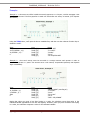
Configuring the SandMath_3x3++ Revision “N”
Plugging the SandMath 3x3 module requires using the bank-switching configuration options on the 41CL (as well as on Clonix/NoVRAM, or the MLDL-2k). For the 41-CL make sure that the six ROM images
are stored in the appropriate block locations in memory (either sRAM or Flash), and that you use the “–
MAX” control string in ALPHA for the execution of the PLUG command.
Hint: the same conventions used for the Advantage Pack are applicable here: place the 3 lower banks
in the first three blocks within a sector, and the 3 upper banks in the 5th , 6th and 7th blocks of the same
sector – thus leaving a “gap” of one block in between, which can be used to store other modules
without a conflict.
P
P
P
Pa
There are only a few new functions in revision 3x3 not included in the 2x2, but they alone account for
two additional banks (one on each page, lower and upper). The difference is therefore substantial,
despite the apparent sameness between revisions. You may of course choose which one to use,
depending on which one is more convenient for your hardware. The optimal setup is the 3x3 revision,
gathering the most benefits from the bank-switching imlpementation (on-line code that doesn’t take
additional footprint). Note that the LASTF features are only available in the 3x3+ verison of the
module.
Note for Advanced Users:
U
Even if the SandMath is a 24k module, it is possible to configure only the first (lower) page as an
independent bank-switched 4k-ROM. This may be helpful when you need the upper port to become
available for other modules (like mapping the CL’s MMU to another module temporarily); or
permanently if you don’t care about the High Level Math (Special Functions) and Statistics sections.
Think however that the FAT entries for the Function launchers are in the upper page, so they’ll be gone
as well if you use the reduced foot-print version (effective 4k only) of the SandMath.
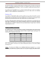
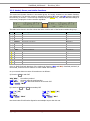
Page
Bank-1
Bank-2
Bank-3
Upper
High-Level Math, Stats
Function Launchers,
Curve Fitting
HP Advantage Solve
& Integrate
Lower
SandMath_44
FRC, HYP, RCL# Math
TVM$, AECROM
Geometry Solvers
Note that it is not possible to do it the other way around; that is plugging only the upper page of the
module will be dysfunctional for the most part and likely to freeze the calculator– do not attempt.
Note: Make sure that revision “N” (or higher) of the Library#4 module is installed.
(c) Ángel M. Martin
Page 8 of 167
December 2014
SandMath_44 Manual - Revision 3x3++
SandMath_44 Module – Revision 3x3++
Math Extensions for the HP-41 System
1. Introduction.
Simply put: here’s the ultimate compilation of MCODE Math functions and FOCAL applications to extend
the native function set of the HP-41 system. At this point in time - way over 30 years after the
machine’s launch - it’s more than likely not realistic to expect them to be profusely employed in FOCAL
programs anymore - yet they’ve been included for either intrinsic interest (read: challenging MCODE or
difficult to realize) or because of their inherent value for those math-oriented folks.
This module is a record-breaking 24k implementation, arranged in a dual bank-switched configuration.
The lower pages include more general-purpose functions, re-visiting the usual themes: Fractions, Base
conversion, Hyperbolic functions, RCL Math extensions, Triangles and Circles, as well as simple-butneat little gems to round off the page. In sum: all the usual suspects for a nice ride time.
The upper pages delve into deeper territory, touching upon the special functions, approximation theory,
and Probability/Statistics. Some functions are plain “catch-up” for the 41 system (sorely lacking in its
native incarnation), whilst others are a divertimento into a tad more complex math realms. All in all a
mixed-and-matched collection that hopefully adds some value to the legacy of this superb machine –
for many of us the best one ever.
I am especially thankful for the essential contributions from Jean-Marc Baillard: more than 3/4ths of
this module are directly attributable to his original programs, one way or another.
Wherever possible the 13-digit OS routines have been used throughout the module – ensuring the
optimal use of the available resources to the MCODE programmer. This prevents accuracy loss in
intermediate calculations, and thus more exact results. For a limited precision CPU (certainly per today’s
standards) the Coconut chip still delivers a superb performance when treated nicely.
The module uses routines from the Page#4 Library (a.k.a. “Library#4”). Many routines in the library
are general-purpose system extensions, but some of them are strictly math related, as auxiliary code
repository to make it all fit in an 8k footprint factor - and to allow reuse with other modules. This is
totally transparent to the end user, just make sure it is installed in your system and that the revisions
match. See the relevant Library#4 documentation if interested.
Function Launchers and Mass key assignments.
As any good “theme” module worth its name, the SandMath has its own mass-Key assignment routine
(MKEYS). Use it to assign the most common functions within the ROM to their dedicated keys for a
convenient mapping to explore the functions. Besides that, a distinct feature of this module is the
function launchers, used to access diverse functions grouped by categories. These include the
Hyperbolic, the Fractions, the RCL Math, and the Special Function groups. This saves memory registers
for key assignments, whilst maintaining the standard keyboard available also in USER mode for other
purposes.
This is the eighth incarnation of the SandMath project, which in turn has had a fair number of revisions
and iterations on its own. One distinct addition has been a secondary Function address Table (FAT) to
provide access to many more functions, exceeding the limit imposed by the operating system (64
functions per page). Some other refinements consisted in a rationalization of the backbone
architecture, as well as a more modular approach to each of pages of the module. Gone are the “8k”
and “12k” distinctions of the past – as now the Matrix and Polynomial functions have an independent
life of their own in separate modules, like the SandMatrix - more on that to come.
(c) Ángel M. Martin
Page 9 of 167
December 2014
SandMath_44 Manual - Revision 3x3++
Conventions used in this manual.
This manual is a more-or-less concise document that only covers the normal use of the functions. All
throughout this manual the following convention will be used in the function tables to denote the
availability of each function in the different function launchers:
[*]:
[F]:
[H]:
[F]:
[RC]:
[CR];
[HK]:
[]:
[$]:
assigned to the keyboard by
direct execution from the main launcher
executed from the hyperbolic launcher
executed from the fractions launcher
executed from the RCL# launcher,
executed from the Carlson Launcher
executed from the Hankel launcher
executed from the Statistics Menu,
sub-function in the secondary FAT.
MKEYS
FL
-HYP
-FRC
-RCL
(no separate function exists)
(no separate function exists)
–ST/PRB
F$
MKEYS prompts for the asiign/de-assign action; use the Y/N keys or back arrow to cancel. There are a
total of 25 functions assigned, refer to the SandMath overlay for details. Note that MKEYS is
programmable as well.
U
U
Xtra Bonus:- High Rollers Game.
There is an Easter egg included in the SandMath 3x3 – hidden somewhere there’s a rendition of the
High Rollers game, so you can relax in between hard-thinking sessions of math, really! There was
simply too much available space in bank 3 of the upper page to leave it unused, so this 500+ bytes
MCODE rendition of the game (written by Roos Cooling, see PPCJ V14 N2 p31) was begging to be
included. As to how to access it… the discovery is part of the enjoyment :-) Hint: even if it’s not
geometric, it certainly is a “Solver”, of a [SHIFT]’ed type…
,
Choose any combination from the available digits on the right which sum matches the target on the
left, repeating until there’s no more digits left (YOU WIN) or there aren’t possible combinations (YOU
LOSE). Use R/S to proceed, back-arrow to delete digits. The game will ask you to try again and will
keep the count of the scores.
,
Finall Disclaimer.With “just” an EE background the author has had his dose of relatively special functions, from college
to today. However not being a mathematician doesn’t qualify him as a field expert by any stretch of the
imagination. Therefore the descriptions that follow are mainly related to the implementation details,
and not to the general character of the functions. This is not a mathematical treatise but just a
summary of the important aspects of the project, highlighting their applicability to the HP-41 platform.
Note: Make sure that revision “N” (or higher) of the Library#4 module is installed.
(c) Ángel M. Martin
Page 10 of 167
December 2014
SandMath_44 Manual - Revision 3x3++
Getting Started: Accessing the Functions.
There are about 230 functions in the SandMath Module. With each of the main two pages containing its
own function table, this would only allow to index 128 functions - where are the others and how can
they be accessed? The answer is called the “Multi-Function” groups.
Multi-Functions F# and F$ provide access to an entire group of sub-functions, grouped by their
affinity or similar nature. The sub-functions can be invoked either by its index within the group using
F#, or by its direct name, using F$. This is implemented in such a way that they are also
programmable, and can be entered into a program line using a technique called “ non-merged
functions”.
You may already be familiar with this technique, originally developed by the HEPAX programmers. In
the HEPAX there were two of those groups; one for the XF/M functions and another for the HEPAX/A
extensions. The PowerCL Module also contains its own, and now the SandMath joins them – this time
applied to the mathematical extensions, particularly for the Special Functions group.
A sub-function catalog is also available, listing the functions included within the group. Direct execution
(or programming if in PRGM mode) is possible just by stopping the catalog at a certain entry and
pressing the XEQ key. The catalog behaves very much live the native ones in the machine: you can
stop them using R/S, SST/BST them, press ENTER^ to move to the next “sub-section”, cancel or
resume the listing at any time.
As additional bonus, the sub-function launcher F$ will also search the “main” module FAT if the subfunction name is not found within the multi-function group – so the user needn’t remember where a
specific function sought for was located. In fact, F$ will also “find” a function from any other pluggedin module in the system, even outside of the SandMath module.
Main Launcher and Dedicated (Secondary) Launchers.
The Module’s main launcher is [FL]. Think of it as the trunk from which all the other launchers stem,
providing the branches for the different functions in more or less direct number of keystrokes. With a
well-thought out logic in the functions arrangement then it’s much easier to remember a particular
function placement, even if its exact name or spelling isn’t know, without having to type it or being
assigned to any key.
Despite its unassuming character, the FL prompt provides direct access to many functions. Just press
the appropriate key to launch them, using the SandMath Overly as visual guide: the individual functions
are printed in BLUE, with their names set aside of the corresponding key. They become active when the
“F: _” prompt is in the display.
, or
Besides providing direct access to the most common Special Functions, FL will also trigger the
dedicated function launchers for other groups. Think of these groupings as secondary “menus” and
you’ll have a good idea of their intended use. The following keys activate the secondary menus:
[A], activates the STAT/PRB menus.
[H] and [O], activate the Hankel and Carlson groups launchers respectively
[0] , activates the FRC (Fractions) launcher; [,] (Radix) activates the LastFunction
[SHIFT] switches into the hyperbolic choices; pressing it twice enables the second overlay.
[ALPHA] and [PRGM] activate the F$ andF# sub-functions launchers respectively
[USER] activates the TVM$ launcher (latest addition to the module)
[<-], back-arrow cancels it or returns to it from a secondary menu.
(c) Ángel M. Martin
Page 11 of 167
December 2014
SandMath_44 Manual - Revision 3x3++
As it occurs with standard functions, the name of the launched function will be shown on the display
while you hold the corresponding key – and NULLED if kept pressed. This provides visual feedback on
the action for additional assurance.
This is a good moment to familiarize yourself with the [FL] launcher. Go ahead and try it, using it also
in PRGM mode to enter the functions as program lines. Note that when activating F$ you’ll NOT need
to press [ALPHA] a second time to spell the sub-function name (unlike standard functions like COPY, or
XEQ). This saves keystrokes as you can start spelling the function name directly. You still need to press
[ALPHA] to terminate the sequence.
Direct-access function keys:
U
[A]:
UStat/Prob MENUSUU
[B]:
Euler’s Beta Function
[C]:
Digamma (PSI)
[D]:
Rieman’s Zeta Function
[E]:
Gamma Natural log
[F]:
One over Gamma
[G]:
Euler’s Gamma Function
[H]:
UHankel’s LauncherUU
[I]:
Bessel I(n,x)
[J]:
Bessel J(n,x)
[SHIFT]: UHyperbolics LauncherUU
[K]:
Bessel K(n,x)
[L]:
Bessel Y(n,x)
[M]:
Lambert’s W
[SST]: Incomplete Gamma
[N]:
Root Finder
[O]:
UCarlson Launcher U
[R]:
Exponential integral
[S]:
Numeric integral
[X]:
Polygamma (PsiN)
[V]:
Cosine Integral
[W]:
Spherical Y(n,x)
[Z]:
Sine Integral
[=]:
Spherical J(n,x)
[?]:
Incomplete Beta
[0]:
UFractions Launcher
[R/S]: View Mantissa
[,]:
Activates the Last Function
[ALPHA]:Sub-function Alpha launcher,F$
[ON]: Turns the calculator OFF
[USER]: Time Value of Money launcher, TVM$
[PRGM]: Sub-function UIndex Launcher, F#
[<-]: Cancels out to the OS or retruns from 2nd.
A green “H” on the overlay prefixing the function name represents the Hyperbolic functions. This also
includes the Hyperbolic Sine and Cosine integrals, in addition to the three “standard” ones. Using the
[SHIFT] key will toggle between the direct and inverse functions. Pressing [<-] will take you back to
the main F: prompt. Note that the RCL Math functions are also linked to the main launcher, to invoke
them use the [RCL] launcher, sort of “Hyper-RCL” thus need to press: [FL], [HYP] to get the
“RCL# _ _” prompt.
Typically the secondary launchers have the possible choices in their prompt; we’ll see them later on.
The STAT menu differs from the others in that it consists of two line-ups toggled with the [SHIFT] key
– providing access to 10 functions using the keys in the top-row directly below the function symbol.
The Fractions functions are encircled by a red line on the overlay, at the bottom and left rows of the
keyboard. They include the fraction math, plus a fraction Viewer and fraction/Integer tests. The Hankel
and Carlson launchers present their choices in their prompts, and will be covered in a dedicated
section later in the manual.
(c) Ángel M. Martin
Page 12 of 167
December 2014
SandMath_44 Manual - Revision 3x3++
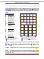
Appendix 0.- The “Hyper-SHIFT” keyboard. (HYP”)
The available room in the auxiliary banks has proven useful to extend the HYP launcher beyond the
strictly hyperbolic functions. Presing the [SHIFT] key twice activates the “hyper-SHIFT” mode; and then
repeat pressings of [SHIFT] will toggle between the normal and hyper-Shift modes:
----------
The hyper-SHIFT extensions are mainly about adding a SHIFTED HYP mode with a full keyboard of
“assignments”, like those for functions assigned by MKEYS to the HYP prompt choices.
The picture below shows the function map for the [HYP] and [SHIFT-HYP] launchers (HYP”). As it’s
now customary, the [SHIFT] key will toggle between these two, and the back arrow will return to the
main FL launcher.
Note that this arrangement includes both main- and sub-functions in the same second-layer keyboard.
This is a very convenient way to circumvent the inability to directly assign sub-functions to keys. Later
on in the manual we’ll see dedicated launchers for other subfunctions in the CARLSON and HANKEL
sections – completing the round.
[A]:
Prime FactorsUU
[B]:
Discrete Hartley Transform
[C]:
Curve Fitting
[D]:
Rieman’s Zeta (Borwein)
[E]:
Poly-Logarithm
[F]:
Fourier Series
[G]:
Inverse Gamma
[H]:
Inverse Hyp SINEUU
[I]:
Inverse Hyp COS
[J]:
Inverse Hyp TAN
[SHIFT]: UTToggles Hyp LaunchersUU
[K]:
Days between Dates
[L]:
Cubic Equation Roots
[M]:
Shortcut to RCL Launcher
[SST]: ATAN2 (Complex argument)
[N]:
INPUT data in registers
[O]:
UTaylor Series U
[P]:
Arithmetic-Geometric Mean
[<-]: Cancels out to [FL]
[Q]:
Probability Distribution Function
[R]:
Generalized Exponential Integral
[S]:
Generalized Error Function
[T]:
Inverse Error Function
[U]:
Cumulative Probability Function
[V]:
Hyperbolic Sine Integral
[W]:
Whittakert Function M
[X]:
Lobachesvsky function
[Y]:
Inverse Cumulative Probability
[Z]:
Hyperbolic Sine Integral
[=]
Clausen function
[?]
Straight Line Equation
[:]
Reg Maximum
[;]
Stack Sort
(c) Ángel M. Martin
[Spc]
[R/S]
Register Sort
Ceiling function
Page 13 of 167
December 2014
SandMath_44 Manual - Revision 3x3++
This implementation effectively supersedes the MKEYS approach, respecting the default keyboard (no
need to toggle USER mode) and without the extra KA registers consumption. Note also that the HYP”
keyboard is compatible with the SandMath Overlay - of which finally real-life units were made!. Perhaps
it’s time for a second overlay... 
The “Last Function” functionality.
The latest releases of the SandMath and SandMatrix modules include support for the “LASTF”
functionality. This is a handy choice for repeat executions of the same function (i.e. to execute again
the last-executed function), without having to type its name or navigate the different launchers to
access it.
The implementation is not universal – it only covers functions invoked using the dedicated launchers,
but not those called using the mainframe XEQ function. It does however support two scenarios: (a)
functions in the main FATs, as well as (b) those sub-functions from the auxiliary FATs. Because the
latter group cannot be assigned to a key in the user keyboard, the LASTF solution is especially useful in
this case. The following table summarizes the launchers that have this feature:
Module
SandMath 3x3+
revision “M”
revision “N”
Launchers
FL, HYP, FRC, RCL#
F$ _
F# _ _ _
FCAT (XEQ’)
LASTF Method
Captures sub/fnc id#
Captures sub/fnc NAME
Captures sub/fnc id#
Captures sub/fnc id#
Note that the Alphabetical launcher F$ will switch to ALPHA mode automatically. Spelling the function
name is terminated pressing ALPHA, which will either execute the function (in RUN mode) or enter it
using two program steps in PRGM mode by means of the F# function plus the corresponding index
(using the so-called non-merged approach). This conversion happens entirely automatically.
The LASTF operation is also supported when excuting a sub-function from within the FCAT
enumeration, using the [XEQ] hot-key - which is very handy for those with elusive spelling. Another
new enhancement is the display of the sub-function names when using the index-based launcher F# which provides visual feedback that the chosen function is the intended one (or not). This feature is
active in RUN mode, when entering it into a program, and when single-stepping a program execution but obviously not so during the standard program runs.
LASTF Operating Instructions
No separate function exists - The Last Function feature is triggered by pressing the radix key (decimal
point - the same key used by LastX) while the launcher prompts are up. This is consistently
implemented across all launchers supporting the functionality in the three modules (SandMath,
SandMatrix and PowerCL) – they all work the same way.
When this feature is invoked, it first briefly shows “LASTF” in the display, quickly followed by the lastfunction name. Keeping the key depressed for a while shows “NULL” and cancels the action. In RUN
mode the function is executed, and in PRGM mode it’s added as a program step if programmable, or
directly executed if not programmable.
The functionality is a two-step process: a first one to capture the function id#, and a second that
retrieves it, shows the function name, and finally parses it. All launchers have been enhanced to store
the appropriate function information (either index codes or full names) in registers within a dedicated
buffer (with id# = 9). The buffer is maintained automatically by the modules (created if not present
when the calculator is ‘switched ON), and its contents are preserved while it is turned off (during “deep
sleep”). No user interaction is required.
(c) Ángel M. Martin
Page 14 of 167
December 2014
SandMath_44 Manual - Revision 3x3++
If no last-function information yet exists, the error message “NO LASTF” is shown. If the buffer #9 is
not present, the error message is “NO BUF” instead.
Appendix 1.- Launcher Maps.
The figures below provide a better overview, illustrating the hierarchy between launchers and their
interconnectivity. For the most part it is always possible to return to the main launcher pressing the
back arrow key, improving so the navigation features – rather useful when you’re not certain of a
particular function’s location.
The first one is the Main SandMath Launcher.
The first mapping doesn’t show all the direct execute function keys. Use the SandMath overlay as a
reference for them (names written in BLUE aside the functions).
Note that FL$ requires pressing [ALPHA] a second time in order to type the sub-function name.
And here’s the Enhanced RCL MATH group:
Here all the prompts expect a numeric entry. The two top rows keys can be used as shortcuts for 1-10.
Note that No STK functionality is implemented – even if you can force the prompt at the IND step.
Typically you’ll get a “DATA ERROR” message - Rather not try it :- )
(c) Ángel M. Martin
Page 15 of 167
December 2014
SandMath_44 Manual - Revision 3x3++
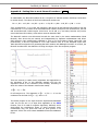
Function index at a glance.
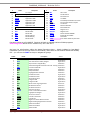
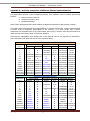
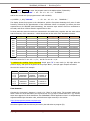
And without further ado, here’s the list of functions included in the module. First the main functions:
#
0
1
2
3
4
5
6
7
8
9
10
11
12
13
14
15
16
17
18
19
20
21
22
23
24
25
26
27
28
29
30
31
32
33
34
35
36
37
38
39
40
41
42
43
44
45
46
47
48
Name
-SNDMTH 3x3
2^X-1
1/N
DGT
N^X
AINT
ATAN2
BS>D
CBRT
CEIL
CHSYX
CROOT
CVIETA
D>BS
D>H
E3/E+
FLOOR
SOLVER
GEU
H>D
HMS*
HMS/
LOGYX
MKEYS
P>R
QREM
QROOT
QROUT
R>P
R>S
S>R
STLINE
T>BS _ _
VMANT
X^3
X=1?
X=YR?
X>=0?
X>=Y?
Y^1/X
Y^^X
YX^
-FRC _
D>F
F+
FF*
F/
FRC?
(c) Ángel M. Martin
Description
#
TAYLOR sub-function
Powers of 2
Harmonic Numbers
Sum of mantissa digits
Geometric Sums
Alpha Integer Part
Dual-argument ATAN
Base to Decimal
Cubic Root
Ceil function
CHSY by X
Cubic Equation Roots
Driver for CROOT
Decimal to Base
Dec to Hex
1,00X
Floor Function
Geometric and TVM Solvers
Euler's Constant
Hex to Dec
HMS Multiply by scalar
HMS Divide by scalar
LOG b of X
Mass Key Assgn.
Complete P-R
Quotient Reminder
2nd. Degree Roots
Ouput Roots
Complete R-P
Rectangular to Spheric
Spheric to Rectangular
Straight Line from Stack
Dec to Base
View Mantissa
X^3
Is X 1?
Is X~Y? (rounded)
is X>=0?
is X>=Y?
Xth. Root of Y
Extended Y^X
Modified Y^X
Fraction Math Launcher
Decimal to Frac
Fraccion Addition
Fraction Substract
Fraction Multiply
Fraction Divide
is X fractional?
0
1
2
3
4
5
6
7
8
9
10
11
12
13
14
15
16
17
18
19
20
21
22
23
24
25
26
27
28
29
30
31
32
33
34
35
36
37
38
39
40
41
42
43
44
45
46
47
48
Name
-HL MATH+
1/GMF
FL
F$
F#
BETA
CHBAP
CI
DHST
EI
ENX
ERF
FFOUR
FINTG
FLOOP
FROOT
GAMMA
HCI
HGF+
HSI
IBS
ICBT
ICGM
IERF
IGMMA
JBS
KBS
LINX
LNGM
LOBACH
PSI
PSIN
SI
SJBS
SYBS
TAYLOR
WL0
YBS
ZETA
ZETAX
-PB/STS _
%T
CORR
COV
"CURVE"
EVEN?
GCD
LCM
LR
Page 16 of 167
Description
Displays "RUNNING…"
Reciprocal Gamma Cont..Frc.
Function Launcher
Launcher by Name
Launcher by index
Beta Function
Chebyshev's Approximation
Cosine Integral
Discrete Hartley Transform
Exponential Integral
Generalized Exponential Integrals
Error Function
Fourier Series
Numerical Integration
Auxiliary function
Solution of f(x)=0
Gamma Function (Lanczos)
Hyperbolic Cosine Integral
Generalized Hypergeometric Funct.
Hyperbolic Sine Integral
Bessel In Function
Incomplete Beta Function
Incomplete Gamma Function
Inverse Error function
Inverse Gamma
Bessel Jn Function
Bessel Kn Function
Polylogarithm
Logarythm Gamma Function
Lobachevsky Function
Digamma Function
Polygamma
Sine Integral
Spherical J Bessel
Spherical Y Bessel
Taylor Polynomial order 10
Lambert W Function
Bessel Yn
Zeta Function (Direct method)
Zeta Function (Borwein)
Displays STAT menu
Total Percentual
Correlation Coefficient
Sample Covariance
Curve Fitting (AECROM)
is X Even?
Greatest Common Divisor
Least Common Multiple
Linear Regression
December 2014
SandMath_44 Manual - Revision 3x3++
#
49
50
51
52
53
54
55
56
57
58
59
60
61
62
63
Name
INT?
-HYP _
HACOS
HASIN
HATAN
HCOS
HSIN
HTAN
-RCL _
AIRCL
RCL^
RCL+
RCLRCL*
RCL/
Description
Is X Integer?
Hyberbolics Launcher
Hypebolic ACOS
Hyperbolic ASIN
Hyperbolic ATAN
Hyperbolic COS
Hyperbolic SIN
Hyperbolic TAN
Extended Recall
ARCL Integer Part
Recall Power
Recall Add
Recall Subtract
Recall Multiply
Recall Divide
#
49
50
51
52
53
54
55
56
57
58
59
60
61
62
63
Name
LRY
NCR
NPR
ODD?
PDF
PFCT
PRIME?
RAND
RGMAX
RGSORT
RGSUM
SEEDT
ST<>
STSORT
TVM$
Description
LR Y-value
Combinations
Permutations
Is X Odd?
Probability Distribution Function
Prime Factorization in Alpha
Is X Prime?
Random Number
Block Maximun
Register Sort
Register Sum
Stores Seed for RNDM
Exchange ST & REG
Stack Sort
Time Value of Money Launcher
Functions in blue are all in MCODE. Functions in black are MCODE entries to FOCAL programs.
Pink background denote new in revisions 3x3, 3x3+ and 3x3++
And now the sub-functions within the Special Functions Group – deeply indebted to Jean-Marc’s
contribution (and not the only section in the module). Note there are two sections within this auxiliary
FAT – you can use the FCAT hot keys to navigate the groups.
index#
0
1
2
3
4
5
6
7
8
9
10
11
12
13
14
15
16
17
18
19
20
21
22
23
24
25
26
27
Name
-SP FNC
#BS
#BS2
AIRY
ALF
AWL
DAW
DBY
HGF
HK1
HK2
HNX
ITI
ITJ
JNX1
KLV
KLV2
KUMR
LERCH
LI
LNX
LOMS1
LOMS2
RCWF
RHGF
SHK1
SHK2
SIBS
(c) Ángel M. Martin
Description
Cat header - does FCAT
Author
Ángel Martin
Aux routine, All Bessel
Ángel Martin
Aux routine 2nd. Order, Integers
Ángel Martin
Airy Functions Ai(x) & Bi(x)
JM Baillard
Associated Legendre function 1st kind - Pnm(x) JM Baillard
Inverse Lambert W
Ángel Martin
Dawson integral
JM Baillard
Debye functions
JM Baillard
Hypergeometric function
JM Baillard
Hankel1 Function
Ángel Martin
Hankel2 Function
Ángel Martin
Struve H Function
JM Baillard
Integral if IBS
Ángel Martin
Integral of JBS
Ángel Martin
Bessel Jn for large arguments
Keith Jarret
Ber & Bei functions
JM Baillard
Ker & Kei functions
JM Baillard
Kummer Function
Ángel Martin
Lerch Transcendent function
JM Baillard
Logarythmic Integral
Ángel Martin
Struve Ln Function
JM Baillard
Lommel s1 function
JM Baillard
Lommel S2
JM Baillard
Regular Coulomb Wave Function
JM Baillard
Regularized hypergeometric function
JM Baillard
Spherical Hankel1
Ángel Martin
Spherical Hankel2
Ángel Martin
Spherical IBS
Ángel Martin
Page 17 of 167
December 2014
SandMath_44 Manual - Revision 3x3++
28
29
30
31
32
33
34
35
36
37
38
39
40
41
42
43
`44
45
46
47
48
49
50
51
52
53
54
TMNR
WEBAN
WHIM
WL1
ZOUT
-ELLIPTIC
AJF
BRHM
CLAUS
CRF
CRG
CRJ
CSX
ELIPF
ELP
HERON
JEF
LEI1
LEI2
LEI3
PP2
SAE
THETA
THV
VMOD
VXA
V*A
Toronto function
Weber and Anger functions
Whittaker M function
Lambert W1
Output Complex to ALPHA
Section Header
Aux for JEF
Area of cyclic quadrilateral (Bhramagupta)
Clausen Function
Carlson Integral 1st. Kind
Carlson Integral 2nd. Kind
Carlson Integral 3rd. Kind
Fresnel Integrals, C(x) & S(x)
Elliptic Integral
Perimeter of Ellipse
Area of Triangle (Heron formula)
Jacobian Elliptic functions
Legendre Elliptic Integral 1st. Kind
Legendre Elliptic Integral 2nd. Kind
Legendre Elliptic Integral 3rd. Kind
Point-to-Point Distance
Surface Area of an Ellipsoid
Theta Functions (1,2,3,4)
Tetrahedron Volume
Vector Module
Vector Cross Product
Vector Dot Product
JM Baillard
JM Baillard
Ángel Martin
Ángel Martin
Ángel Martin
n/a
JM Baillard
JM Baillard
JM Baillard
JM Baillard
JM Baillard
JM Baillard
JM Baillard
Ángel Martin
Ángel Martin
JM Baillard
JM Baillard
JM Baillard
JM Baillard
JM Baillard
Ángel Martin
JM Baillard
JM Baillard
JM Baillard
Ángel Martin
Ángel Martin
Ángel Martin
The following section groups the factorial functions, circling back from the special functions into the
number theory field - a timid foray to say the most.
index#
55
Name
Description
-FACTORIAL
AGM
APNB
BN2
CPF
DSP?
ERFN
FFCT
ICPF
LOGHF
LOGMF
MANTXP
MFCT
NPRML
POCH
PRML
PSD
QTNL
SFCT
XFCT
Section Header
Arithmetic-Geometric Mean
Apery Numbers
Bernouilly Numbers
Cumulative probability (,
Display Digits setting
Generalized Error Function
Falling Factorial
Inverse Cumulative Prob.
Logarithm Hyper-Factorial
Logarithm Multi-Factorial
Mantissa
Multi-Factorial
Number Primorials
Pochhammer symbol
Prime PrImorials
Poisson Standard Distribution
Quantile (Standard Normal ICP)
Super Factorial
Extended Factorial
(c) Ángel M. Martin
Page 18 of 167
56
57
58
59
60
61
62
63
64
65
66
67
68
69
70
71
72
73
74
Author
n/a
Ángel Martin
JM Baillard
Ángel Martin
Ángel Martin
Ángel Martin
JM Baillard
Ángel Martin
Ángel Martin
Ángel Martin
JM Baillard
David Yerka
JM Baillard
Ángel Martin
Ángel Martin
Ángel Martin
Ángel Martin
Ángel Martin
JM Baillard
Ángel Martin
December 2014
SandMath_44 Manual - Revision 3x3++
And the last section takes us into the Transforms and Approximation theory, very loosely speaking:
index#
75
Name
76
77
78
79
80
81
82
83
84
85
86
87
88
89
90
91
92
93
94
95
96
-TRANSFORM
^LIST
ANUMDL
b*e
b<>e
CDAY
CdT
CHB
CHB2
CHBCF
CRVF
D%
DAYS
DHT
dPL
IN
INPUT
JDAY
OUT
PDEG
PL
-/+
dB+
REV
FCAT
97
98
99
Description
Section Header
Input Data in List
ANUM with Deletion
Array size from control word
index swapping
Calendar Day
Aux for CHBAP
Chebyshev Polinomials 1st. Kind
Chebyshev Polinomials 2nd. Kind
Chebyshev's Coefficients
Curve Fitting (AECROM)
Difference Percent
Days between Dates
Discrete Hartley transform
First derivative of Polynomial
Input Data in Registers
Data input as ALPHA Lists
Julian Day Number
Output Data from Registers
Polyn degree from control word
Polynomial Evaluation
Calculates (Y-X)/(Y+X)
Decibel Addition
Shows Module revision
Function Catalog
Author
n/a
Ángel Martin
HP Co.
Ángel Martin
Ángel Martin
Ángel Martin
JM Baillard
JM Baillard
JM Baillard
JM Baillard
Nelson F. Crowle
Ángel Martin
HP Co.
JM Baillard
Ángel Martin
Ángel Martin
Ángel Martin
Ángel Martin
Ángel Martin
JM Baillard
Ángel Martin
Ángel Martin
Ángel Martin
Ángel Martin
Ángel Martin
(*) The best way to access FCAT is through the main launcher [FL] , then pressing [SHIFT] ENTER^ (“N”)
FCAT provides usability enhancements for admin and housekeeping. It invokes the sub-function
CATALOG, with hot-keys for individual function launch and general navigation . Users of the POWERCL
Module will already be familiar with its features, as it’s exactly the same code – which in fact resides in
the Library#4 and it’s reused by both modules and the SandMatrix as well.
U
The hot-keys and their actions are listed below:
U
[R/S]:
[SST/BST]:
[SHIFT]:
[XEQ]:
[ENTER^]:
[<-]:
halts the enumeration
moves the listing one function up/down
sets the direction of the listing forwards/backwards
direct execution of the listed function – or entered in a program line
moves to the next/previous section depending on SHIFT status
back-arrow cancels the catalog
One limitation of the sub-functions scheme that you’ll soon realize is that, contrary to the standard
functions, they cannot be assigned to a key for the USER keyboard . Typing the full name (or entering
its index at the FL# prompt) is always required. This can become annoying if you want to repeatedly
execute a given sub- function.
The LAST Function implementation certainly reduces this issue for repeat executions of the last subfunction called, without a dedicated key assignment required. Another work-around consists of writing
a micro-FOCAL program with just the sub-function as a single pair of program lines, and then assign it
to the key of choice. Not perfect but it works.
(c) Ángel M. Martin
Page 19 of 167
December 2014
SandMath_44 Manual - Revision 3x3++
2. Lower-Page Functions in detail
The following sections of this document describe the usage and utilization of the functions included in
the SandMath_44 Module. While some are very intuitive to use, others require a little elaboration as to
their input parameters or control options, which should be covered here. Reference to the original
author or publication is always given, for additional information that can (and should) also be
consulted.

U
U
2.1.1. Elementary Math functions
Even the most complex project has its basis – simple enough but reliable, so that it can be used as
solid foundation for the more complex parts. The following functions extend the HP-41 Math function
set, and many of them will be used either as MCODE subroutines or directly in FOCAL programs.
[*]
[*]
[*]
[*]
[*]
[*]
[*]
[*]
[*]
[*]
Function
2^X-1
1/N
N^X
ATAN2
CBRT
CEIL
CHSYX
E3/E+
FLOOR
GEU
LOGYX
QREM
X^3
Y^1/X
Y^^X
YX^
Description
Self-descriptive, faster and better precision than FOCAL
Harmonic Number H(n)
Geometric Sums
Two-argument arctangent (complex argument)
Cubic root (main branch)
Ceiling function of a number
Multiple CHS by Y
Index builder
Floor function of a number
Euler-Mascheroni constant
Base-Y Natural logarithm of X
Quotient Remainder
Cube power of X
x-th root of Y
Very large powers of X (result >= 1E100)
Modified Y^X (does 0^0=1)
Author
Ángel Martin
Ángel Martin
Ángel Martin
Ángel Martin
Ángel Martin
Ángel Martin
Ángel Martin
Ángel Martin
Ángel Martin
Ángel Martin
Ángel Martin
Ken Emery
Ángel Martin
Ángel Martin
Ángel Martin
JM Baillard

2^X-1 provides a more accurate result for smaller arguments than the FOCAL equivalents. It
will be used in the ZETAX program to calculate the Zeta function using the Borwein algorithm.

1/N calculates the Harmonic number of the argument in X, that is the sum of the
reciprocals of the natural numbers (which excludes zero) lower and equal to n. It will be used
in the calculation of the Kelvin functions and the Bessel functions of the second kind, K(n,x)
and Y(n,x).

Example: calculate H(5) and H(25). Use the main FL launcher and the LastF functionality.
5, FL [SHIFT] [F]
25, FL , [ , ]
(c) Ángel M. Martin
=> 2.283333333
=> 3.815958178
Page 20 of 167
December 2014
SandMath_44 Manual - Revision 3x3++

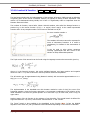
N^X Calculates a generalized value of the Faulhaber’s formula for integer values of x. – The
few first integer values of x have explicit formulas for the result, but that’s not the case for a
general value, which can also be non-integer. Obviously for x=-1 this function returns identical
results than the previous one, albeit slower due to the additional complexity of the term.
Example: Check the triangular (x=1) and pyramidal (x=2) formulas for n=10 – which are
particular cases of the Faulhaber’s Formula, involving Binomial coefficients and Bernoulli’s
numbers. See the link below for details: http://en.wikipedia.org/wiki/Faulhaber%27s_formula
10, ENTER^, 1, FL [SHIFT] [A]
10, ENTER^, 2, FL [ , ]
=> 55.00000000
=> 385.0000000
And using the convention B(1) = 0.5 the formula is:
Which can be programmed using a few of the SandMath functions, albeit it will be considerably slower
due to the impact of the Zeta algorithms (part of Bernoulli’s) – kicking in for n>4.

CHSYX is related to the same subject, and in general relevant to the summation of
alternating series – It can be regarded as an extension of CHS but dependent of the number in
X. Its expression is:
CHS(y,x)= y*(-1)^x, and thus changing the sign of Y when the number in X is odd.

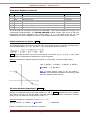
ATAN2 is the two-argument variant of arctangent. Its expression is given by the following
definitions:
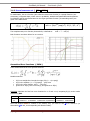
Example: Calculate ATAN2(, 2) using the main FL launcher.
PI , PI , 2 , * , FL [SHIF]-[SHIFT] [SST]
=> 1.107148718
Those amongst you with a penchant for complex variable would no dobut recognize this as the
principal value of the argument of the logarithm of a complex number.
(c) Ángel M. Martin
Page 21 of 167
December 2014
SandMath_44 Manual - Revision 3x3++

E3/E+ does just what its name implies: adds one to the result of dividing the argument in x
by one-thousand. Extensively used throughout this module and in countless matrix programs,
to prepare the element indexes.

FLOOR and CEIL . The floor and ceiling functions map a real number to the largest previous
or the smallest following integer, respectively. More precisely, floor(x) = [x] is the largest
integer not greater than x and ceiling(x) = ]x[ is the smallest integer not less than x.
The SandMath implementation uses the native MOD function, through the expressions:
CEIL (x) = [x – MOD(x, -1)];
and
FLOOR (x) = [x – MOD(x, 1)].

GEU is a new constant added to the HP-41: the Euler-Mascheroni constant, defined as the
limiting difference between the harmonic series and the natural logarithm:
The numerical value of this constant to 10 decimal places is:  = 0.5772156649… The stack lift
is enabled, allowing for normal RPN-style calculations. It appears in formulas to calculate the 
(Psi) function (Digamma) and the Bessel functions of 2 nd. Kind, amongst others.

LOGYX is the base-b Logarithm, defined by the expression below where the base b is
expected to be in register Y, and the argument in register X.
Example: verify that 5.55 = Log[2, 2^(5.55)] using 2^X-1 and LOGXY:
5.55, 2^X-1 , 1, + , 2, X<>Y , LOGYX

=> 5.55000000
QREM Calculates the Remainder “R” and the Quotient “Q” of the Euclidean division between
the numbers in the Y (dividend) and X (divisor) registers. Q is returned to the Y registers and
R is placed in the X register. The general equation is: Y = Q X + R, where both Q and R are
integers. Note that if the dividend is smaller than the divisor the function will return zero for
the quotient, and the remainder will be the divisor itself
Example: calculate the remainder and quotient of dividing 27 over 4.
27, ENTER^, 4, F$ “QREM”
=> X=3 (remainder); Y= 6 (quotient)
Since we used the Alpha-Launcher in this example, we can take advantage of the LASTF
feature to repeat the operation with swapped values:
4, ENTER^, 27, FL [ , ]
(c) Ángel M. Martin
=> X=4 ; Y=0
Page 22 of 167
December 2014
SandMath_44 Manual - Revision 3x3++

CBRT calculates the cubic root of a number. Note that this could also be done using the
mainframe function Y^X with Y=1/3 for positive values of X, but unfortunately it results in
DATA ERROR when X<0 – and therefore the need for a new function.
Obviously it follows that CBRT(-x) = - CBRT(x), for x>0

Y^1/X
and
X^3
are purely shortcut functions, which clearly are equivalent to
{ 1/X, Y^X }, and to { X^2, LASTx, * } respectively - but with additional precision due to
the 13-digit intermediate calculations. Besides it does away with the pesky (and totally
unjustified) issue present with negative numbers as base in Y^X.
Example: verify in two different ways that the cubic root of (-3)^3 is indeed -3.
3 , CHS , X^3 , CBRT
3 , CHS , X^3 , 3 , Y^1/X
=> -3.000000000
=> -3.000000000

Y^^X is used to calculate powers exceeding the numeric range of the calculator, simply
returning the base in X and the exponent in Y. The result is shown in ALPHA in RUN mode.For instance calculate 85^69 to obtain:

YX^ is a modified form of the native Y^X function, with the only difference being its
tolerance to the 0^0 case – which results in DATA ERROR with the standard function but here
returns 1. This has practical applications in FOCAL programs where the all-zero case is just to
be ignored and not the cause for an error.

XFCT is an extended-range factorial, capable of displaying results over the standard numeric
range of th calculator. Like Y^^X above, it returns the mantissa to X and the exponent to
the Y-register. This function resides in the secondary FAT, and therefore needs to be called
using any of the launchers. The implementation is just a particular case of the super-factorial,
with the repeat factor p=1. This will be described in the corresponding section later on.
Example: to calculate 70! and 120! just type: (using FIX 6 for display formatting)
70, F$ “XFCT”
120, FL [ , ]
=> 1.197857 E100
=> 6.689503 E198
The full value of the mantissa is left in the X register.
(c) Ángel M. Martin
Page 23 of 167
December 2014
SandMath_44 Manual - Revision 3x3++
2.1.2. Number Displaying, Bases and Coordinate Conversions.
A basic set of base conversions and diverse number displaying functions round up the elementary set:
[F$]
[*]
[*]
[*]
[*]
[F]

Function
DGT
AINT
DSP?
HMS/
HMS*
MANTXP
P>R
R>P
R>S
S>R
VMANT
Description
Sum of Mantissa digits
A fixture: appends integer part of X to ALPHA
Shows current decimal digits setting
HMS Division by scalar
HMS Multiplication by scalar
Mantissa and Exponent of number
Modified Polar to Rectangular, <) in [0, 360[
Modified Rectangular to Polar, <) in [0, 360[
Rectangular to Spherical
Spherical to Rectangular
Shows full-precision (10-digit) mantissa
Author
Ángel Martin
Frits Ferwerda
Ángel Martin
Tom Bruns
Tom Bruns
David Yerka
Tom Bruns
Tom Bruns
Ángel Martin
Ángel Martin
Ken Emery
DGT is a small divertimento useful in pseudo-random numbers generation. It simply returns
the sum of the mantissa digits of the argument – at light-blazing speed using just a few
MCODE instructions. More about random numbers will be covered in the Probability/Stats
section later on.
Example: calculate the sum of all digits of the HP-41’s rendition of PI:
PI, XEQ “DGT”

=> 40.000000000
DSP? (also in the secondary FAT) returns in X the number of decimal places currently set in
the display mode 0 regardless whether it’s FIX, SCI , or END. Little more than a curiosity, it can
be used to restore the initial settings under program control after changing them for displaying
or formatting purposes.

AINT elegantly solves the classic dilemma to append an index value to ALPHA without its
radix and decimal part - eliminating the need for FIX 0, and CF 29 instructions, taking extra
steps and losing the original calculator settings. Note that HP added AIP to the Advantage
module, and the CCD has ARCLI to do exactly the same.

MANTXP and VMANT are related functions that deal with the mantissa and exponent parts
of a number. MANTXP places the mantissa in X and the exponent in Y, whereas VMANT
shows the full mantissa for a few instants before returning to the normal display form - or
permanently if any key is pressed and held during such time interval , similar to the HP-42S
implementation of “SHOW”.

R>P and P>R are modified versions of the mainframe functions R-P and P-R. The
difference lies in the convention used for the arguments in Polar form, which here varies
between 0 and 360, as opposed to the –180, 180 convention in the mainframe.
Example: convert the point [-1, -1] to the modified polar coordinates and back to rectangular:
DEG, 1, CHS, ENTER^, R>P
X<>Y
X<>Y, P>R
(c) Ángel M. Martin
=> 1.414213562
=> 225.0000000 (and not -135)
=> original point
Page 24 of 167
December 2014
SandMath_44 Manual - Revision 3x3++

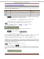
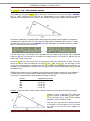
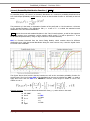
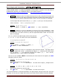
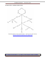
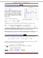
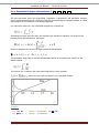
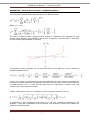
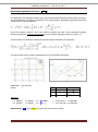
R>S and S>R contine with the coordinate conversion theme. This pair of functions can be
used to change between rectangular and spherical coordinates.
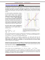
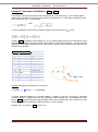
The convention used is shown in the figure
below, defining the origin and direction of
the azimuth and polar angles as referred to
the rectangular axis: { r, phi, theta } <-> {
x, y, z }
The SandMath implementation makes use of
the fact that with the appropriate selection
of origins, dual P-R conversions are
equivalent to Spherical, and vice-versa.
Example: convert the rectangular point [1, 2, 3] to spherical coordinates, and then back to
rectangular:
3, ENTER^, 2, ENTER^, 1, R>S
RDN
RDN
RDN, RDN, S>R
=>
=>
=>
=>
r = 3.741657386 (*)
phi = 0.640522313
theta = 1.107148718
original point in stack.
(*) You can also use function VMOD in the secondary FAT to check the modulus result. Its
value should be slightly more accurate, as it uses direct math routines not based on [TOPOL].

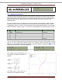
HMS* and HMS/ complement the arithmetic handling of numbers in HMS format, adding
to the native HMS+ and HMS- pair. They multiply or divide the HH.MMSSSS value in Y by an
scalar in X. As it’s expected, the result is also put in HMS format as well.
Example: calculate the triple of 2 hours, 45 minues and 25 seconds
2,4525, ENTER^, 3, XEQ “HMS*”
=> 8.161499999
That is 8 hours, 16 minutes and 15 seconds almost exactly.
This function is useful in surveying calculations, as a shortcut of the standard approach involving
conversion to decimal format prior to the operation. Note that to multiply or divide two numbers
given in HMS format you need to convert them both to rdecimal form using HR, perfrom the
operation and convert the result back to HMS format to end.
(c) Ángel M. Martin
Page 25 of 167
December 2014
SandMath_44 Manual - Revision 3x3++
Entering the base conversion section - The following functions are available in the SandMath:
Function
BS>D
D>BS
D>H
H>D
T>BS _ _
[*]
[*]
[*]
Description
Base to Decimal
Decimal to base in Y
Decimal to Hex
Hex to Decimal
Base-Ten to Base, prompting version.
Author
George Eldridge
George Eldridge
William Graham
William Graham
Ken Emery

The first two are FOCAL programs, taken from the PPC ROM. They are the generic base-b
to/from Decimal conversions. The Direct conversion D>BS expects the base in Y and the
decimal number in X, returning the base-b result in Alpha. The inverse function BS>D uses
the string in Alpha and the base in X as arguments. You can chain them to end with the same
decimal number after the two executions.

T>BS (Ten to Base) is the MCODE equivalent to D>BS, much faster and more elegant due
to its prompt – where in RUN mode you input the destination base. The result is shown in the
display and also left in ALPHA, so it could be also used by BS>D (once the base is in X). Note
that the original argument (decimal value) is left in X unaltered, so you can use T>BS
repeated times changing the base to see the results in multiple bases without having to reenter the decimal value.
T>BS is programmable. In PRGM mode the prompt is ignored and the base is expected to be in the Y
register, much the same as its FOCAL counterpart D>BS. Obviously using zero or one for the base will
result in “DATA ERROR”. The maximum base allowed is 36 – and the custom error message “BASE>36”
will be shown it that’s exceeded (note that larger bases would require characters beyond “Z”).
The maximum decimal value to convert depends on the destination base, since besides the math
numeric factors; it’s also a function of the Alpha characters available (up to “Z”) and the number of
them in the display (length <=12). For b=16 the maximum is 9999 E9, or 0x91812D7D600
T>BS is an enhanced version of the original function, also included in Ken Emery’s book “MCODE for
Beginners”. The author added the PRGM-compatible prompting, as well as some display trickery to
eliminate the visual noise of the original implementation. Also provision for the case x=0 was added,
trivially returning the character “0” for any base. The prompt can be filled using the two top keys as
shortcuts, from 1 to 10 (A-J), or the numeric keys 0-9.
Direct DEC<>HEX Conversion.
Because of its importance in computer science, the dec to hexadecimal conversions have dedicated
MCODE functions in the SandMath, D>H and H>D . Use them to convert the number in X to its
Hex value in Alpha, and vice-versa. Both functions are mutually reversed, and H>D does an stack lift
as well.
The maximum number allowed is 0x2540BE3FF or 9,99999999 E9 decimal - much smaller than with
T>BS, so there’s a price to pay for convenience.
These functions were written by William Graham and published in PPCJ V12N6 p19, enhancing in turn
the initial versions first published by Derek Amos in PPCCJ V12N1 p3.
(c) Ángel M. Martin
Page 26 of 167
December 2014
SandMath_44 Manual - Revision 3x3++
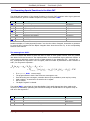
2.1.3. First, Second and Third degree Equations.
A MCODE implementation of these offers no doubt the ultimate solution, even if it doesn’t involve any
high level math or sophisticated technique. The Stack is used for the coefficients as input, and for the
roots as output. No data registers are used.
[*]
[*]
[*]
Function
STLINE
QROOT
QROUT
CROOT
CVIETA

Description
Calculates straight line coefficients from two data points
Calculates the two roots of the equation
Displays the roots in X and Y
Calculates the three roots of the equation
Driver program for CROOT
Author
Ángel Martin
Ángel Martin
Ángel Martin
Ángel Martin
Ángel Martin
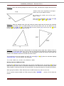
STLINE is a simple function to calculate the straight line coefficients from two of its data
points, P1(x1,y1) and P2(x2,y2). The formulas used are:
B
B
B
B
Y = ax +b, with:
a= (y2-y1)/(x2 –x1),
B
B
B
B
B
B
B
B
b = y1 – a x1
and
B
B
B
B
It is trivial to obtain the root once a and b are known, using: x0 = -b/a
B
B
Example: Get the equation of the line passing through the points (1,2) and (-1,3)
U
U
3, ENTER^, -1, ENTER^, 2, ENTER^, 1, STLINE
and its root is left in register Z:
RDN, RDN
=> Y: 2,500; X: -0,500
=> 5,000
(*) will be shown in RUN mode only

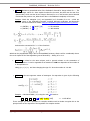
QROOT . The general forms of the Quadratic Equation is:
with a#0 .
Given the quadratic equation above, QROOT calculates its two solutions (or roots). You need to input
the three coefficients into the stack registers: Z, Y, X using: a, ENTER^, b, ENTER^, c
The roots are obtained using the well-known formula: X1,2 = -b/2a +- sqrt[(-b/2a)^2 – c/a]
Depending on the sign of the discriminant (i.e. the argument of the square root) the result will be real
or complex roots. If the discriminant is positive then the roots are real, and their values x1 and x2 will
be left in Y and X registers upon execution. Register Z will contain a non-zero value, which can be used
in program mode to determine the case.
Example: Calculate the roots of the equation: x^2 + 2x -3 =0
1, ENTER^, 2, ENTER^, 3, CHS, QROOT
=> x1= 1, x2= -3
In RUN mode the SandMath will show both values in the display, separated by the ampersand sign.
Moreover, should the values be integers then the representation will omit the superfluous decimal
places:
(c) Ángel M. Martin
Page 27 of 167
December 2014
SandMath_44 Manual - Revision 3x3++
If the discriminant is negative, then the roots z 1 and z2 are complex and conjugated (symmetrical over
the X axis), with Real and Imaginary parts defined by:
B
B
B
Re(Z) = -b/2a
Im(Z) = sqrt[abs((-b/2a)^2 –c/a)]
B
z1 = Re(z) + i Im(z)
z2 = Re(z) – i Im(z)
B
B
B
B
Upon execution reg-Z will be zero (used in Programs), Im(z) will be left in Y and Re(z) will be left in X.
In RUN mode the display will show the first root in a composite format showing one of the roots.
Example: Calculate the roots of the equation: x^2 + x + 1 = 0
1, ENTER^, ENTER^, QROOT
RDN

=> Re(z) = -0.500000000
=> Im(z) = 0.866025404
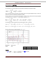
CROOT The general forms of the Cubic Equation is:,
with a#0
Given the cubic equation above, CROOT calculates the three solutions (or roots). You need to input
the four coefficients in the stack registers T, Z, Y, X using:
a, ENTER^, b, ENTER^, c, ENTER^, d, ENTER^
CROOT uses the well-known Cardano-Vieta formulas to obtain the roots. The highest order coefficient
doesn’t need to be equal to 1, but errors will occur if the first term is zero (for obvious reasons).
The SandMath implementation does reasonably well with multiple roots, but sure enough you can find
corner-cases that will make it fail - yet not more so than an equivalent FOCAL program. Appendix 2
lists the code, as well as an equivalent FOCAL program to compare the sizes (much shorter, but surely
much slower and with data registers requirements
Both functions can return real or complex roots. If the roots are complex, the functions will flag it in the
following manners:
1. QROOT will clear the Z register, indicating that X and Y contain the real and imaginary parts of
the two solutions. Conversely, if Z#0 then X and Y contain the two real roots.
2. CROOT will leave the calculator in RAD mode, indicating that X and Y contain the real and
imaginary parts of the second and third roots. The real root will always be placed in the Z
register. Conversely, if the calculator is set in DEG mode then registers Z,Y, and X have the
three real roots.
3
2
Example1: Calculate the three solutions of the equation: x + x + x + 1 = 0
U
P
U
1, ENTER^, ENTER^, ENTER^ , CROOT
P

P
P
Z: -1,000; Y: 1,000; X: 1 E-10
, Shown as rounded number for the real part.
(c) Ángel M. Martin
Page 28 of 167
December 2014
SandMath_44 Manual - Revision 3x3++
Example 2:- Calculate the roots of the equation: ƒ(x) = 2x3 − 3x2 − 3x + 2.
U
U
P
2, ENTER^, -3, ENTER^, ENTER^, 2, CROOT
P
P
P
-> Z: 0,500; Y: -1,000; X: 2,000
From the final prompt you know all roots are real, since the two last roots are real and the first one
must always be real in a cubic equation.
The value in Z blinks briefly in the display before the final prompt above is presented; use RCL Z (or
RDN, RDN) to retrieve it. No user registers are used.
QROUT outputs the contents of the X and Y registers to the display, interpreted by the value in Z to
determine whether there are tow real roots or the Real & Imaginary parts of the complex roots. It will
be automatically invoked by QROOT (all cases) and by CROOT (real roots) when they are executed in
RUN mode. Note that CROOT will not display the (first) real root, which will be located in Z.
CVIETA is a driver program for CROOT, including the prompts for the equation coefficients. The
results are placed in the stack, following the same conventions explained above. See the program
listing below showcasing the use of a few SandMath functions.
(c) Ángel M. Martin
Page 29 of 167
December 2014
SandMath_44 Manual - Revision 3x3++
Appendix 2.- CVIETA equivalent FOCAL program, replaced now with an all-MCODE implementation.
01
02
03
04
05
06
07
08
09
10
11
12
13
14
15
16
17
18
19
20
21
22
23
24
25
26
27
28
29
30
31
32
33
34
35
36
37
38
39
40
41
42
43
44
45
46
47
48
49
50
51
52
53
54
55
56
57
58
59
60
61
62
63
LBL "CVIETA"
-AMC MATH
R^
ST/ T (0)
ST/ Z (1)
/
STO 00
RDN
STO 01
RDN
3
/
STO 02
X^3
ST+ X (3)
RCL 01
RCL 02
*
RCL+ (00)
2
/
STO 03
X^2
RCL 01
RCL 02
X^2
3
*
STO 01
3
/
X^3
+
X<=0?
GTO 01
SQRT
ENTER^
ENTER^
RCL 03
CBRT
STO 01
X<>Y
CHS
RCL 03
CBRT
STO 03
+
RCL 02
"X1"
ARCL X (3)
AVIEW
STO 00
RCL 01
RCL 03
3
SQRT
*
64
65
66
a'2/a'3 in T
67
a'1/a'3 in Z
68
69
a0 = a'0 / a'3
70
71
a1 = a'1 / a'3
72
a2 = a'2 / a'3
73
74
75
a2/3
76
a2^3/27
77
2*a2^3/27
78
a1
79
a2/3
80
a1*a2/3
81
2*a2^3/27 - a1*a2/3
82
Showing off… :-)
83
84
85
a0/2 + a2^3/27 - a1*a2/6
86
(a0/2 + a2^3/27 - a1*a2/6)^2
87
a1
88
a2/3
89
a2^2/9
90
91
a2^2/3
92
a1-a2^2/3
93
a1-a2^2/3
94
95
1/3 (a1 - a2^2/3)
96
1/27 (a1 - a2^2/3)^3
97
1/27 (a1 - a2^2/3)^3 + (a0/2 + a2^3/27 - a1*a2/6)^298
99
yes, all real roots
100
complex roots
101
102
RPLX
103
a0/2 + a2^3/27 - a1*a2/6
104
105
106
cbrt(+x-R3/2)
107
108
109
a0/2 + a2^3/27 - a1*a2/6
110
111
112
cbrt(-x-R3/2)
113
114
a2/3
115
116
117
118
119
real root
120
cbrt(+x-R3/2)
121
cbrt(-x-R3/2)
122
123
124
125
126
"Running" message
(c) Ángel M. Martin
Page 30 of 167
2
/
RCL 01
RCL 03
+
2
/
CHS
RCL 02
,
STO T (0)
RDN
QROUT
STO 01
X<>Y
STO 02
RTN
LBL 01
DEG
LASTX
CHS
SQRT
ST+ X (3)
X#0?
1/X
RCL 03
ST+ X (3)
CHS
*
ACOS
3
/
STO 03
LASTX
E3/E+
STO 05
RCL 01
3
/
CHS
SQRT
ST+ X (3)
STO 04
LBL 08
RCL 03
COS
RCL 04
*
RCL 02
"X"
AIRCL
5
"|-="
ARCL X(3)
AVIEW
STO IND 05
120
ST+ 03
ISG 05
GTO 08
END
imaginary part
cbrt(+x-R3/2)
cbrt(-x-R3/2)
a2/3
real part
flag it as Complex
Z=0 indicates it
all real roots
a0/2 + a2^3/27 - a1*a2/6
a0 + 2*a2^3/27 - a1*a2/3
1,003
a1-a2^2/3
a1/3-a2^2/9
a2^2/9 - a1/3
2*SQR(a2^2/9 - a1/3)
a2/3
Alpha integer REG
05
December 2014
SandMath_44 Manual - Revision 3x3++
2.1.4. Additional Tests: Rounded and otherwise.
Ending the first section we have the following additional test functions:
Function
X=1?
X>=Y?
X>=0?
X=YR?
FRC?
INT?
EVEN?
ODD?
ZOUT
[*]
[*]
[*]
[*]
[F]
[F]
Description
Is X (exactly) equal to 1?
Is X equal to or greater than Y?
Is X equal to or greater than zero?
Rounded Comparison
Is X a fractional number?
Is X an integer number?
Is X an even integer?
Is X an odd integer?
Combines the values in Y and X into a complex result
Author
Nelson C. Crowle
Ken Emery
Ángel Martin
Ángel Martin
Ángel Martin
Ángel Martin
Ángel Martin
Ángel Martin
Ángel Martin
They follow the general rule, returning YES / NO in RUN mode, and skipping a program line if false in a
program. Their criteria are self-explanatory for the first three. These functions come very handy to
reduce program steps and improve the legibility of the FOCAL programs.

X>=Y? compares the values in the X and Y registers, skipping one line if false.

X>=0? compares with zero the value in the X register, skipping one line if false.
These functions are arguably “missing” on the mainframe set; a fact partially corrected with the indirect
comparison functions of the CX model (X>=NN?), but unfortunately not quite the same.

X=1? is a quick and simple way to check whether the value in X equals one. As usual,
program execution skips one step if the answer is false.

X=YR? establishes the comparison of the rounded values of both X and Y, according to the
current decimal digits set in the calculator. Use it to reduce the computing time (albeit at a loss
of precision) when the algorithms have slow convergence or show oscillating results for larger
number of decimals.

INT? and FRC? are two more test functions which criteria is the integer or fractional nature
of the number in X. Having them available comes very handy for decision branching in FOCAL
programs. The Fractions section of the module is the natural placement for them.

EVEN? and ODD? Test the divisibility by 2 of the number in X, i.e. whether it is an even or
an odd number. For non-integer values the fractional part will be ignored in the test.

ZOUT has been used in FOCAL programs in the SandMath, - Its most interesting features are
perhaps displaying integer values (in either real or imaginary parts) without any decimals; as
well as omitting them when equal to zero (showing “Z=0” if both are null).
(c) Ángel M. Martin
Page 31 of 167
December 2014
SandMath_44 Manual - Revision 3x3++

U

2.2.1. Fraction Arithmetic and Displaying.
A rudimentary set of fraction arithmetic functions is included in the SandMath, including the four basic
operations plus a fraction viewer and two test functions.
[*]
[F]
[F]
[F]
[F]
[F]
[F]
[F]
Function
-FCR
D>F
F+
FF/
F*
FRC?
INT?
Description
Fractions Launcher
Calculates a fraction that gives the number in X
Fraction addition
Fraction subtraction
Fraction multiplication
Fraction division
Is X a fractional number?
Is X an integer number?
Author
Ángel Martin
Frans de Vries
Ángel Martin
Ángel Martin
Ángel Martin
Ángel Martin
Ángel Martin
Ángel Martin
D>F is the key function within this group. Shows in the display the smallest possible fraction that
results in the decimal number in X, for the current display precision set. Change the display precision as
appropriate to adjust the accuracy of the results.
U
U
This means the fraction obtained may be different depending on the settings, returning different
results. For example, the following approximations are found for :




~
~
~
~
104348/33215
355/113
333/106
22/7
in
in
in
in
FIX
FIX
FIX
FIX
9, FIX 8 and FIX 7
6, FIX 5 and FIX 4
3
2, FIX 1 and FIX 0
This function was written by Frans de Vries, and published in DataFile, DF V9N7 p8. It uses the same
algorithm as the PPC ROM “DF” routine.
As per the fraction arithmetic functions, there’s not much to say about them – apart from the fact that
they use the four stack levels to enter both fractions components (the inputted values are expected to
be all integers), and return the numerator and denominator of the result fraction in registers Y and X
respectively. In RUN mode the execution continues to show the fraction result in ALPHA, according to
the currently set number of decimals (see below).
The fraction arithmetic functions can be used in chained calculations, there’s no need to re-enter the
intermediate results, and the Stack enabled makes unnecessary to press ENTER^. Notice that fractions
are entered using the Numerator first.
To re-calculate the fraction after changing the decimal settings just press the divide key, followed by
D>F to re-generate the fraction values.
For example calculate 2/7 over 4/13, then add 9/17 to the result.
2, ENTER^, 7, ENTER^, 4, ENTER^, 13, F/ , 9 ENTER^, 17, F+  347/238
(c) Ángel M. Martin
Page 32 of 167
in FIX 6 mode.
December 2014
SandMath_44 Manual - Revision 3x3++
Needless to say the fractional representation display will not be produced in PRGM mode, but it’ll have
a silent execution instead.
Note that the fraction math functions operate on integer numbers in the stack, returning also the
numerator and denominator as integers. To get the decimal number just execute / to divide them.
In fact that’s exactly what the functions do in RUN mode: upon completion the fraction is “converted”
to a decimal number, then D>F presents the final output. That’s why the display settings determine
the accuracy of the conversions, even if it’s not obviously seen.
This has the advantage that the result is always reduced to the best possible fit . For instance, when
calculating 2/4 plus 18/24 in program mode – with the four values in the stack – the result will be 120
in Y and 96 in X (thus 120/96). However on RUN mode (or SST’ing the program) will show the reduced
fraction:
A good way to check that the result is expressed in irreducible form is pressing GCD, verifying that the
result is indeed 1; try it out if you’re curious.
If you want to see the reduced result from a program execution you’ll need to add program steps to
perform the division and add a conversion to fraction after the fraction-math operation step. The code
snippet below describes this (see lines 10 and 11):
01
02
03
04
05
06
07
08
09
10
11
12
*LBL "TEST"
2
ENTER^
4
ENTER^
18
ENTER^
24
F+
/
D>F
END
INT? and FRC? are two more test functions which criteria is the integer or fractional nature of the
number in X. Having them available comes very handy for decision branching in FOCAL programs. The
Fractions section of the module is the natural placement for them.
The answer is YES / NO depending on whether the condition is true or false. In program mode the
following line is skipped it the test is false.
Note: Make sure that revision “N” (or higher) of the Library#4 module is installed.
(c) Ángel M. Martin
Page 33 of 167
December 2014
SandMath_44 Manual - Revision 3x3++

U
U
2.3.1. Hyperbolic Functions.
Yes there are many unanswered questions in the universe, but certainly one of them is why, oh why,
didn’t HP-MotherGoose provide a decent set of MCODE hyperbolic functions in the (otherwise pathetic)
MATH-PAC, and worse yet -adding insult to injury- how come that error wasn’t corrected in the
Advantage ROM?
For sure we’ll never know, so it’s about time we move on and get on with our lives – whilst correcting
this forever and ever. The first incarnation of these functions came in the AECROM module; I believe
programmed by Nelson C. Crowle, a real genius behind such ground-breaking module - but it was also
somehow limited to 10-digit precision. The versions in the SandMath all use internally13-digit routines.
[*]
[H]
[H]
[H]
[H]
[H]
[H]
Function
-HYP
HSIN
HCOS
HTAN
HASIN
HACOS
HATAN
Description
Hyperbolic Launcher
Hyperbolic Sine
Hyperbolic Cosine
Hyperbolic Tangent
Inverse Hyperbolic Sine
Inverse Hyperbolic Cosine
Inverse Hyperbolic Tangent
Author
Ángel Martin
Ángel Martin
Ángel Martin
JM Baillard
Ángel Martin
Ángel Martin
JM Baillard
The use of function launchers permits convenient access to these six functions without having to assign
them to any key in USER mode. Efficient usage of the keyboard, which can double up for other
launchers or the standard USER mode assignment if that’s also required. Combining the FL and the
SHIFT keys does the trick in a clean and logical way.
and inverses:
The formulas used are well known and
don’t require any special consideration to
program.
The SINH code is also used as a
subroutine for the Digamma function.
(c) Ángel M. Martin
Page 34 of 167
December 2014
SandMath_44 Manual - Revision 3x3++
The direct functions are basically exponentials,
whilst the inverses are basically logarithms.
Both cases are well covered with the mainframe
internal math routines without any need to worry
about singularities or special error handling.
For all hyperbolic functions the input value is expected in X, and the return value will also be left in X.
The original argument is saved in LASTx. No data registers are used.
Examples:
U
Complete the table below, calculating the inverses of the results to compare them with the original
arguments. Use FIX 9 to see the complete decimal range.
HMKEYS assigns -HYP to the [SHIFT] key for convenience
x
1
1,001
0.01
0.0001
10
HSIN
1,175201194
1,176744862
0,010000167
0,000100000
11013,23287
HASIN
1,000000000
1,001000000
0,010000000
0,000100000
10,00000000
HCOS
1,543080635
1,544256608
1,000050000
1,000000005
11013,23292
HACOS
1,000000000
1,001000000
0,009999958
0,000100000
10,00000000
HTAN
0,761594156
0,762013811
0,009999667
0,000100000
0,999999996
HATAN
0,761594156
1,001000000
0,010000000
0,000100000
10,00271302
By now you’ve become an expert in the HYP launcher and for sure appreciate its compactness – lots of
keystrokes!
With a couple of exceptions it’s a100% accuracy to 10 decimal places – and really the only sore point is
in the point 0.001 for HACOS. But don’t worry, there’s no bugs creating havoc here – it’s just the
nature of the beast, bound to occur with the limited precision (even using 13-digits) in the Coconut
CPU.
No wonder you’re going to repeat the same table for the trigonometric functions and see how it stacks
up, right?
While you’re at it, go ahead and calculate the power of two of the square root, pressing:
FIX
9
, 2 , SQRT ,
X^2 , but don’t call HP to report a bug!
For very small arguments the accuracy of SINH and COSH will also start showing incorrect digits.
However HTAN (and HATAN) use an enhanced formula that will hold the accuracy regardless of how
small the argument is.
Note: Make sure that revision “N” (or higher) of the Library#4 module is installed.
(c) Ángel M. Martin
Page 35 of 167
December 2014
SandMath_44 Manual - Revision 3x3++

U
U
The SandMath Module includes a set of functions written to extend the native RCL functionality –
mainly in the direct math operations missing when compared to the STO equivalents, but also
increasing its versatility and ease of use. There are five new RCL Math functions, plus a launcher to
access them in a convenient and useful way:
[*]
[RC]
[RC]
[RC]
[RC]
[RC]
[RC]
Function
RCL” _ _
RCL+ _ _
RCL- _ _
RCL* _ _
RCL/ _ _
RCL^ _ _
AIRCL _ _
Description
RCL Math Launcher
RCL Plus
RCL Minus
RCL Multiply
RCL Division
RCL Power
ARCL integer Part of number in Register nn
Author
Ángel Martin
Ángel Martin
Ángel Martin
Ángel Martin
Ángel Martin
Ángel Martin
Ángel Martin
2.4.1. Individual Recall Math functions.
The five RCL Math new functions cover the range of four arithmetic operations (like STO does) plus a
new one added for completion sake. The functions would recall the number in the register specified by
the prompt, performing the appropriate math using the value in register X as first argument and the
recalled number as the second argument.
Design criteria for these were:
1. should be prompting functions
2. should support indirect addressing (SHIFT)
3. should utilize the top 2 rows for index entry shortcut
The first condition is easy to implement in RUN mode, as it’s just a matter of selecting the appropriate
prompting bits in the function MCODE name - but it gets very tricky when used under program mode.
This has been elegantly resolved using a method first used by Doug Wilder, by means of using the
program line following the instruction as the index argument. Somewhat similar to the way the HEPAX
implemented it, although here there’s some advantages in that the length of the index argument
doesn’t need to be fixed, dropping leading zeroes and even omitting it altogether if it’s zero (assuming
the following line isn’t a numeric one which could be misinterpreted).
The indirect addressing is actually quite simple, as it simply consists of an offset added to the register
number in the index. All the function code must do is remove it from the entry data provided by the
OS, and the task is done. The offset value is hex 80, or 128 decimal. We’ll revisit this when discussing
the RCL launcher.
And the third objective is provided “for free” by the OS as well, no need for extra code at all – just
using the appropriate prompting bits in the function’s name.
(c) Ángel M. Martin
Page 36 of 167
December 2014
SandMath_44 Manual - Revision 3x3++
Stack arguments are more involved than the indirect addressing. No attempt has been made to use the
mainframe internal routines to accommodate this case, so stack prompts are excluded. Note that even
if the Stack arguments are not directly allowed (controlled by the prompting bits), it is unfortunately
possible to use the decimal key in an indirect register sequence; that is after pressing the SHIFT key.
This won’t work properly in the current design so must be avoided.
2.4.2. RCL Launcher – the “Total Rekall”.
The basic idea of a launcher is a function capable of calling a set of other functions. The grouping in
this case will be for the five RCL Math functions described above, plus logically the standard RCL
operation – inclusive its indirect registers addressing. Other enhancements include the prompt
lengthener to three fields for registers over 99 (albeit this is de-facto limited to 128 as we’ll see later
on).
The keyboard mapping for [RCL] is as follows:






Numeric keypad (or Top rows) to perform the standard RCL
[SHIFT] for Indirect register addresses
[EEX] for the prompt lengthener to three places
[RCL] to revert to the standard RCL function (see note below)
Math keys (+, -, / , *, and ^) to invoke the RCL Match functions
Back arrow to cancel out to the OS
Note that [RCL] is not programmable. This is done intentionally by design, so that it can be used in a
program to enter any of the RCL Math functions directly as a program line (ignoring the corresponding
prompt). Using the [RCL] hot-key reverts to the standard RCL operation. This nifty trick is what you’d
use to register it in a program, as long as the RCL key is not assigned to another function.
U
Notice also that indirect addressing is indeed supported by this scheme: just add hex 80 (that is
decimal 128) to the register number you want to use as indirect register. As simple as that! So RCL+
IND 25 will be entered as the following two program lines: RCL+, followed by 153.
This however effectively limits the usefulness of the prompt lengthener to the range R100 to R127 –
because from R128 and on the index is interpreted as an indirect register address instead . However,
the function will allow pressing SHIF and EEX, for a combination of IND and prompt lengthener
which will work as expected provided that the 128 limit isn’t reached – enough to make your head spin
a little bit!?
U
U
Example: Store 5 in register R101, and 55555,000 in register R5.
U
U
This requires some indirect addressing as well; say using register Y the sequence would be:
101, ENTER^, 5, STO IND Y, and then: 55555, STO 5
Then execute RCL” IND 101 (press RCL”, SHIFT, EEX , 0 , 1 )--> to obtain 55555,00 in X
Note: general-purpose prompt lengtheners are a better alternative to the [EEX] implementation used
here. Their advantage of course is that they are applicable to all mainframe prompting functions, not
only to the enhanced RCL. Thus for instance, you could use it with STO as well, removing the need for
indirect addressing to store 5 in R101. The AMC_OS/X module has a general-purpose prompt
lengthener, activated by pressing the [ON] key while the function prompt is up.
(c) Ángel M. Martin
Page 37 of 167
December 2014
SandMath_44 Manual - Revision 3x3++
Pressing [ALPHA] at the RCL prompt will invoke function AIRCL _ _. This will in turn prompt for a data
register number, and once filled it’ll append the integer part of the value stored in that register to the
ALPHA register – thus equivalent to what AINT does with the x register.
Note that AIRCL _ _ is fully programmable. When entered in a program you’d ignore the prompts,
and the program step following it will be used to hold the register number to be used by ARCLI when
the program runs. This technique is known as “non-merged” functions, to work-around the limitation of
the OS – Too bad we can’t use the Byte Table locations wasted by eG0bEEP and W” instead! This
method is used in several functions of the SandMath module, like the RCL math functions just
described.
Appendix 3.- A trip down to Memory Lane. From the HP-41 User’s Handbook.-
(c) Ángel M. Martin
Page 38 of 167
December 2014
SandMath_44 Manual - Revision 3x3++
Note: Make sure that revision “N” (or higher) of the Library#4 module is installed.
(c) Ángel M. Martin
Page 39 of 167
December 2014
SandMath_44 Manual - Revision 3x3++

U
U
What good is a math–related module without a Triangle solver application? Never too basic to be
unimportant, especially if it can be tucked away in an auxiliary bank and doesn’t take the customary set
of FAT entries – FAT space is always at a premium. Revision 3x3 of the SandMath includes the
AECROM “TRIA”, which can arguably be considered the best Triangle solver ever written for the 41.
And it is incorporated into a new single function that acts as consolidated launcher for it and the other
two geometric solvers. All improved with 13-digit math routines and other usability enhancements.
2.5.1. The three geometric solvers
CIRCLE:
SARR:
TRIA:
different geometric properties of a circle segment.
Slope, Angle, Rise and Run – also connects to the Triangle solver.
Knowing three elements it resolves the other 3 unknown and the area.
Notice that SOLVER can be launched directly from the mail [FL] launcher, using the EEX key as
shortcut.
, and then:
Upon selecting the desired solver, an information message is shortly shown on the display while the
key is held depressed, followed by “NULL” if kept pressed to cancel the action. If not, then the initial
execution of the chosen solver starts always by presenting the default menu of choices – which can
always be recalled by pressing the menu option, on the [E] key
It’s important to mention that these three are FOCAL programs (albeit quite unusual and also stealth to
the FAT) triggering the different choices for these solvers as local labels; therefore the top row keys
should not have any key assignments for this approach to work. Note also that the USER mode will be
activated automatically by the function.
Rather than attempt to explain these functions let’s refer to the original AECROM user’s manual for a
first-hand and inimitable description of their functionality.
1. [ %< ] = SARR- SLOPE. ANGLE. RISE. AND RUN SOLVER
The SARR solver computes slopes, angles, rise and run. Your HP-41 must be in USER mode and, if you
have anything assigned to the top row of keys, you need to clear those assignments.
Example: The slope of a line is .776. What is the angle between the line and level?
Solution: In USER mode, press [XEQ] “SOLVER”, [C] (i.e. SARR), then: 0.776 [A] [B] (37.8115).
When you execute SARR and switch to USER mode, the keys in the top row take on new meanings. To
see these new meanings press the [E] key in the top row at any time. The calculator shows you the
menu:
(c) Ángel M. Martin
Page 40 of 167
December 2014
SandMath_44 Manual - Revision 3x3++
The first four keys in the top row represent the values SLope, ANgle, RIse, and RuN, and the fifth key
calls the menu. Pressing one of the first four keys can mean either "take the value in the X-register as
an input" or "calculate a value," depending on when you press it. When you key in a value and press
one of the first four keys, the HP-41 takes it as an input. But immediately following an input, pressing
one of the first four keys means "compute this value."
In the above example, the only known value was the slope, which is all you need to know to solve for
the angle. You simply keyed in the slope (0.776 [A]) and solved for the angle [B]).
To solve for anyone of the four unknowns, you need to input knowns according to the following table.
To Solve for:
Slope
Angle
Rise
Run
You need to input:
Run and Rise, or Angle·
Run and Rise, or Slope
Run, and Angle or Slope
Rise, and Angle or Slope
IMPORTANT RULE: Always key in your knowns from right to left in the menu.
Example: The center riser on a triangular roof truss is four feet high and the length from one end of
the truss to the midpoint is 22 feet. What is the slope of the roof?
Solution: This solution assumes you have already pressed [XEQ] “SOLVER”, [C]
Now press [E] to view the menu and 22 [D], 4 [C], [A]. The answer is 0.1818.
Example: With a theodolite, you measured the angle of an imaginary line going from the top of a tree
to the ground at a distance of 5.749924998 m (*) from the base of the tree to be 57 degrees. How tall
is the tree?
Assuming you just completed the previous example, press
(remember: you need to be in USER mode, and also in DEG
mode for this example). Then 5.749924998 [D], 57 [B].
[C] will give you the answer (8.854108050 m).
In the above example, you are solving for the Rise given
the Run and the angle (57 degrees). Notice that when you
key in a number before you press a key in the top row, the
calculator takes it as an input. But when you press one of
the top row keys without first keying in a number, the HP41 calculates that value based on the numbers you've just
keyed in.
(*) Converted from the original feet value in the manual.
(c) Ángel M. Martin
Page 41 of 167
December 2014
SandMath_44 Manual - Revision 3x3++
2.
[ <> ] = TRIA - THE TRIANGLE SOLVER.
From SARR, you can press [SHIFT] [d] to execute the TRIA solver, or you can use [XEQ] “SOLVER”,
[A] (i.e. TRIA). TRIA helps you solve all the characteristics of any triangle given three defining
quantities for that triangle. Here's a picture of an arbitrary triangle with its angles and sides labeled:
The sides are labeled in a counterclockwise order around the triangle and the angles are numbered
according to the opposite side. This is the way that TRIA expects a triangle to be oriented. To call up
the TRIA menu execute the function SOLVER, then [A]. Remember, the calculator must be in USER
mode. You will see the menu on the left:
-----
The first three keys in the left-side menu represent the three sides of the triangle, “AR” shows that
using the [D] key you can solve for the AREA of a triangle and the “M” shows you that the [E] key
brings up the menu at any time.
Now press [ ] [e]. You will see the menu on the right side. This is the shifted menu of TRIA. This menu
shows you that by using the shifted top row keys ([ ] [a], [ ] [b], and [ ] [c]), you can input or solve
for any of the three angles of a triangle. Plus, the “^S” selection executes SARR (described before),. So
remember, the TRIA function has two menus. The [E] key calls up the unshifted menu, and [ ] [e] calls
the shifted menu.
TRIA has fairly specific rules for inputting the three knowns that define a triangle. Once the triangle is
oriented similar to the previous diagram (sides labeled counterclockwise), the known values need
to be input in counterclockwise order around the triangle as follows:
Knowns
SSS
ASA
SAS
SAA
SSA
Suggested input order
S1, S2, S3
A3, S2, A1
S1, A3, S2
S1, A3, A1
S1, S2, A1
Example 1: Solve for all the unknown sides, unknown angles, and the area of the following triangle:
Solution: 5.3 [A], 3.1 [B], 83 [ ] [c]. Then press
[ ] [a] to solve for A1 (64.9903), [ ] [b] to solve
for A2 (32.0097), [C] to solve for S3 (5.8048),
and [D] to solve for AREA (8.1538).
Once you have input the three defining knowns
of a triangle, you can change one or two values
at a time to see how the other lengths are
affected.
(c) Ángel M. Martin
Page 42 of 167
December 2014
SandMath_44 Manual - Revision 3x3++
Example 2: Given the following triangle with three known sides, calculate all the angles and the area of
the triangle.
Solution: This is a S S S problem, so the input
order is S1, S2, S3. With 4.24 as S1:
A1 = 20.44°, A2 = 46.25°, A3 = 113.31°, and
AREA = 17.07.
Here are the keystrokes: 4.24 [A], 8.77 [B],
11.15 [C], [ ] [a], [ ] [b], [ ] [c], [D].
Example 3: Given the triangle below (left side) with two known angles and one known side, calculate
the unknowns. Solution: This is an ASA problem, thus the input order is A3, S2, A1. With 15 as S2,
press 65 [ ] [c], 15 [B], 75 [ ] [a]. Then press [A] to see S1 (22.54), [C] to see S3 (21.15), [ ] [b] to
see A2 (40°), and [D] to see the area (153.22).
Example 4: Calculate the unknown characteristics of the triangle above (right side). Solution: This is a
SSA problem, so the input order is S1. S2. A1. Once you have input this problem the calculator displays
the warning “ANGL.SIDE.SIDE”, indicating that this combination of inputs can result in more than one
solution. The calculator solves for the case where A2 is acute.
The keystrokes to input the triangle are 435.7 [A], 452.9 [B], 67 [ ] [a]. After the calculator displays
“ANGL.SIDE.SIDE”. you can solve for the unknowns:
73.11 =A2; 39.89 =A3; 303.58 = S3; 63.280.40 = AREA
Moving between SARR and TRIA.
Pressing the [ ][d] key from the TRIA menu will execute the SARR function, and pressing [ ] [d] from
SARR will execute TRIA. Data are transferred between the two functions as follows: When going from
TRIA to SARR. S1 becomes RUN and S2 becomes RISE. The slope and angle are calculated accordingly.
When going from SARR to TRIA. RUN becomes SI, RISE becomes S2, and A3 is set to 90.
If you transfer between SARR and TRIA using the [XEQ] “SOLVER” ... process, all the data are
cleared.
(c) Ángel M. Martin
Page 43 of 167
December 2014
SandMath_44 Manual - Revision 3x3++
3. [ ( ) ] = CIRC - THE CIRCLE SOLVER
The CIRC solver allows you to calculate properties of a circle and a sector of that Circle from a known
radius and central angle. Like the SARR and TRIA cases, the CIRC solver is menu driven. The following
diagram shows you some of the properties of a circle that can be calculated using CIRC:
Important: The radius (Rd). the sector angle (AN<), and the X- distance (Xd) are the only allowed
inputs. You can also calculate the circumference (CI) of the circle, the area (AR) of the circle, the
segment area (SG), and the sector area (ST).
Three menus are available for CIRC. To view each menu, execute the function ([XEQ] “SOLVER” [B])
and press the [E], [ ][e], and [J] keys.
----
The menu that comes up when you press the
key tells you the meanings of the top row keys,
menu on the [ ][e] key applies to the shifted
row, and the [J] menu tells you the meanings of
keys in the second row.
[E]
the
top
the
Example 1: Calculate the diameter, area, and circumference of a circle with a radius of 10.0. Also,
calculate the arc length, chord length, chord rise, sector area, and segment area of a sector in that
circle with a central angle of 30 degrees.
Solution: With USER mode on and the display set to FIX 4, press SOLVER, [B] (i.e. CIRC),
[E] 10 [A] 30 [B]. Then ...
To calculate
diameter
area
circumference
arc length
chord length
chord rise
sector area
segment area
(c) Ángel M. Martin
Press
[ ][a]
[F]
[ ][c]
[ ][b]
[C]
[ ][d]
[H]
[G]
Result:
_
20.0000
314.1593
62.8319
5.2360
5.1764
0.3407
26.1799
1.1799
Page 44 of 167
December 2014
SandMath_44 Manual - Revision 3x3++
Example 2: Calculate the rise (YR) at X = 1.8. Solution: 1.8 [D] [I] (0.1774)
Notice that the only values you can input are the radius (RA on the [A] key), the central angle (AN on
the [B] key), and the X-distance (XDIS on the [D] key). These values must be knowns if you wish to
calculate any properties that depend upon them.
Geometric Solvers Implementation Details.This section has some comments on the integration to the SandMath - Ignore it altogether if you’re not
interested in what’s going on under the hood.
Adding the AECROM geometric solvers to the SandMath has been an exercise of discovery and
patience. The first due to the appreciation of the ingenuity used by the original developers to integrate
the MCODE accuracy and speed to a basically FOCAL-driven data input process, which relies on the
user flag 22 (DATA Entry flag) as trigger for known / unknown elements.
As mentioned at the beginning of this section, there are three FOCAL programs, which account for all
the possible menu selections made in the three launchers – that is a total of 30 choices. The uncanny
thing about those programs is that for every one and each of them, the same instruction is always
executed – and that instruction is nothing less that the AECROM header function itself.
How then does the function know which option is called up for? The answer lies in the actual program
pointer position of the calling step, thus the relative location of the code was of utmost importance –
which accounts for the patience part, as I had to move and shift large sections of code to
accommodate for the demanding requirements of the FOCAL newcomers.
So there were just about 180 words in the main bank in total, but what a tricky thing to adjust for on
an already-packed module with interdependencies across three banks and two pages...
Fortunately the bulk of the code is the MCODE for SOLVER itself, which has been conveniently located
in bank-3 of the lower page – briefly “coming up” to the main one for the partial key sequence
prompts, and every time the execution ends to the FOCAL program.
I got partial vindication by consolidating the three FOCAL drivers into a single launcher, which
furthermore allowed the removal of the three FAT entries (TRIA, SARR, and CIRC) – a definitive plus
given that the FAT was already full. You can explore those programs switching to PRGM mode during
their execution (in-between entries, standard procedure).
You probably have noticed that I changed the text presented by the different menus to a less-busy
version of the same. Perhaps more importantly, I also swapped the [D] and [ ][d] actions in the TRIA
solver, so now the unshifted [D] calculates the Area. This provides consistency to the [ ][d] key, as the
“gate” to interconnect SARR and TRIA on both cases. Subtle differences, probably just a matter of
taste.
As a side effect of the modification, only one function (MANTXP) was removed from the main FAT; it
has been placed into the auxiliary FAT of the upper page. Hope you agree it was a small price to pay
for such a rewarding addition – definitely worth the extra effort.
(c) Ángel M. Martin
Page 45 of 167
December 2014
SandMath_44 Manual - Revision 3x3++
2.5.2. The Time Value of Money solver.Putting a second yellow ribbon around the box, from revision “M” the SandMath also includes the new
TVM$ solver functionality - taken from the just released TVM ROM. This is an all-MCODE
implementation of the classic functions that rivals with the HP-12C implementation in speed and
accuracy – use it to solve for any of the five money variables with the other four known: N, I, PV, PMT,
and FV.
First of all, accessing the TMV$ solver is also possible using a dedicated entry in the FL launcher –
just press the [USER] key directly at its prompt; thus no need to go through the SOLVER function
even if for consistency reasons it’s also included there. The direct way saves keystroke pressings;
therefore it’s the recommended approach.
Also important to know is that to input the data, TVM$ expects the value already in X before calling
the corresponding menu choice. This is reversed from the geometric solvers, which first present the
prompt with the menu choices for informational purposes (not a launcher).
The same option key is used to either input the variable value or to calculate it based on the other four.
This duality is possible by relying on the status of the user flag 22 (the data entry flag) to determine
whether it’s an input or a calculation action: UF 22 set means input, whereas UF 22 clear means
calculation.
Remember that to actually set the satus of flag 22, you need to press a key on the numeric pad, i.e.
the digits 0-9, the Radix or EEX keys. Any other key will not activate it, in particular RCL, CHS and
ENTER^ - so you need to work around those cases as appropriate when a new value is to be entered.
TVM$ will clear UF 22 upon completion of the command (either inputting or calculating) – this enables
a repeat calculation of different values just by pressing each menu choice in sequence.
After the input or calculation is done, a message will show the result value for the variable chosen. If
the value is an integer number then decimal settings in the calculator will be ignored for further clarity.
Not shown in the main menu are the following actions:

B/E (key [J]) – use it to toggle between BEGIN / END modes. A message is displayed to
inform of the selected mode, and it also toggles UF 00 annunciator in the display as a reminder
of the currently selected mode.

SHOW (keys [F] to [I]) – use it to sequentially review the current values of each of the Money
variables: N, I, PV, PMT, and FV. For additional consistency with the data entering approach,
both B/E and SHOW will also clear UF 22 upon completion.
Rather than attempt to explain the usage and complete functionality let’s borrow the section from the
HP-41 Advantage’s Pac user’s manual – a superb vintage document that avoids re-inventing the wheel.
Bear in mind that whereas the FOCAL version relies on the local keys within the program, the SandMath
implementation uses the TMV$ launcher options for each value input – this is the main difference
between both implementations.
(c) Ángel M. Martin
Page 46 of 167
December 2014
SandMath_44 Manual - Revision 3x3++
The TVM program solves different problems involving time, money, and interest - the compoundinterest functions. The following variables can be inputs or results.

N = the number of compounding periods or payments. (For a 30-year loan with monthly
payments, N = 12 x 30 = 360.)

I = the periodic interest rate as a percent. (For other than annual compounding, this
represents the annual percentage rate divided by the number of compounding periods per
year. For instance, 9% annually compounded monthly equal 9 / 12 = 0 75%)

PV = the present value. (This can also be an initial cash flow or a discounted value of a series
of future cash flows.) Always occurs at the beginning of the first period.

PMT = The periodic payment,

FV = The future value. (This can also be a final cash flow or a compounded value of a series of
cash flows.) Always occurs at the end of the Nth period.
You can specify the timing of the payments to be either at the end of the compounding period (End
mode) or at the beginning of the period (Begin mode). Begin mode sets flag 00. Ending payments are
common in mortgages and direct-reduction loans; beginning payments are common in leasing.
Equation
Where i is the periodic interest rate as a fraction (i = 1/100),
p = 1 in Begin mode or 0 in End made.
Valid Input Values for Data
Use a cash-flow diagram to determine what your cash-flow inputs are and whether to specify them as
positive or negative. The cash-ftow diagram is just a time-line divided into time periods. Cash flows
(transactions) are indicated by vertical arrows: an upward arrow is positive for cash received, while a
downward arrow is negafive for cash paid out.
For example, the six-period time line on the left shows a $20 cash outflow initially and a $50 cash
inflow at the end of the fourth period. (Begn mode cannot be used in calculating PV or FV.) The fiveperiod time line on the right shows a $1,000 cash outflow initially and a $100 inflow at the end of each
period, ending with an additional #1,000 inflow at the end of the fifth period.
(c) Ángel M. Martin
Page 47 of 167
December 2014
SandMath_44 Manual - Revision 3x3++
Instructions.

The program TVM will solve for any one of the variables N, I, PV, PMT, or FV given the other
three or four, which must include either N or I. The order of entry is unimportant. lf you use
only four variables, then the fifth must equal zero. All variables are set to zero when you first
run TVM or clear the financial data, so you do not have to enter a zero in these cases.

You should clear the financial data (.B) before beginning a completely new calculation;
otherwise, previous data that is not overwritten will be used (i.e., for the fourth, unused
variable), Running the program anew also clears the financial data.

Remember to specify cash inflows (arrow up) as positive values and cash outflows (arrow
down) as negative values. The results are also given as positive ox negative, indicating inflow
or outflow.

Check that the payment mode is what you want. If you see the flag 00 annunciator (a small 0
below the main display line), then Begin mode is set. If not, End mode is set. To change the
mode, press [J] (a toggle). The display will then show what you have just set: BEGIN MODE or
END MODE. The default is End-mode (flag 00 clear).

Remember that the interest rate must be consistent with the number of compounding periods.
(An annual percentage rate is appropriate only if the number of compounding periods also
equals the number of years.)

You might want to set the display format for two or three decimal places (FIX 2 / 3).
This menu will show you which key corresponds to
which function in TVM. Press to recall this menu to the
display at any time. This will not disturb the program in
any way.
To clear the menu at any time, press [<-]. This shows
you the contents of the X-register, but does not end
the program. You can perform caIculations, then recall
the main menu by pressing 0. (However, you do not
need to clear the program's display or recall the menu
before performing calculations.)
Remarks
This program uses local Alpha labels (as explained in the owner's manual fox the HP-41) assigned to
keys [A]- [E], and their shifted counterparts (except [ ][c]) and [J]. These local assignments are
overridden by any User-key assignments you might have made to these same keys, thereby defeating
this program. Therefore be sure to clear any existing User-key assigments of these keys before using
this program, and avoid redefining these keys in the future within possible.
The financial varlable keys will only store a value if you enter it from the keyboard. If, for example, you
recall a value from a register then press a variable key, the program wil calculate that variable instead
of storing the recalled value. To store a value that was placed in the X-register by some other means
than actually keying it in, press [STO] before pressing the variable key.
(c) Ángel M. Martin
Page 48 of 167
December 2014
SandMath_44 Manual - Revision 3x3++
Examples
Example 1.- A borrower can afford a $650.00 monthly payment on a 30-year, 14.25% mortgage. How
much can he borrow? The first payment is made one month after the money is loaned. (This requires
End mode.)
Using the TVM$ solver, we’ll input the known variables first, and then use the unknown function key to
obtain the result:
Input
650, CHS
14.25, ENTER^, 12, /
30, ENTER^, 12, *
0
Keys
TVM$,
TVM$,
TVM$,
TVM$,
TVM$,
[D]
[B]
[A]
[E]
[C]
Result
“PMT=-650“
“I=1.1875“
“N=180”
“FV=0”
“PV=53,955.91959“
Example 2.- How much money must be set aside in a savings account each quarter in order to
accumuIate $4,000 in 3 years? The account earns 11% interest, compounded quarterly and deposits
begin immediately
Input
11, ENTER^, 4, /
3, ENTER^, 4, *
4000
0
Keys
TVM$,
TVM$,
TVM$,
TVM$,
TMV$,
TMV$,
[J]
[B]
[A]
[E]
[C]
[D]
Result
“BEGIN MODE“ (sets flag 00)
“I=2.7500“
“N=12”
“FV=4,000”
“PV=0
“PMT=-278,223688”
Notice that when you press a key after keying in a value, the calculator stores that value in the
indicated variable (equivalent to STO into the register). However, when you press it without first keying
in a value, the calculator computes a value for the indicated variable.
(c) Ángel M. Martin
Page 49 of 167
December 2014
SandMath_44 Manual - Revision 3x3++
Programming Information.
The calculation for N, PV, PMT and FV all use a direct formula based on the values for the other four
variables. TVM$ uses 13-digit math routines for extended precision, thus the accuracy should in theory
be better than the FOCAL programs used elsewhere (like the Advantage’s own TVM).
The calculation for the interest rate uses an iterative method to solve the non-explicit equation. This is
done applying Newton’s formula for the successive estimations of the solution, starting with the
following initial value:
i0 = [ abs( PV + n*PMT + FV) ]
1/n
The function’s derivative for Newton’ s formula is calculated using the expression:
2
f ’ (i) = (PMT / i ) * [ (1+i)
-n
- 1 ] + n * [PMT (1 + ip)/i – FV ] * (1+i)
-(n+1)
During the calculation the display shows a blinking message, shortly followed by the calculated result:
and then:
Data Registers.
The usage of data registers in TVM$ is compatible with the other FOCAL programs in the Advantage
Pac (“TVM”) and in the PPC ROM (“FI”). This is convenient if you want to use them interchangeably
to compare the speed and accuracy of the different implementations. You can see the current contents
with the RCL function and the top row keys as arguments, from 01 to 05 as follows:
N–
I–
PV –
PMT –
FV -
R01
R02
R03
R04
R05
When you call TVM$ it first makes a copy of the contents of these data registers into the stack, and
uses those values for the calculations. Upon completion the obtained result is stored in the
corresponding register and left in the X register as well.
Using TVM$ in Programs.
Notice that TVM$ is designed to be used interactively – but it can also be entered in a program
utilizing the merged functions scheme, whereby the specific option is specified as an index (or
argument) in the next program step following TMV$. This will be taken as the “function argument of
the argument in Rnn”, always assuming it is a calculation action and not data input (regardless of the
current status of UF 22). Simply use STO for storing the values in a program.
The valid values for this argument line are logically 0 to 10, corresponding to the same indexes used in
the register allocation and local keys within the menu. Had TVM$ been a sub-function, and therefore
already using 2 steps in a program (F# plus index), you’d appreciate the fact that it’d take three
program lines (and 5 bytes) to access to any of the financial sub-routines! This compounded scheme is
nothing short of amazing, if you ask me…
(c) Ángel M. Martin
Page 50 of 167
December 2014
SandMath_44 Manual - Revision 3x3++
3. Upper-Page Functions in detail.
It’s time now to move on to the second page within the SandMath – holding the Special Functions and
the Statistical and Probability groups. Let’s see first the Statistical section – easier to handle and of
much less extension; and later on we’ll move into high-level math, taking advantage of the extended
launchers and additional functionality described in the introduction of this manual.
.
U
U
The following functions are in this general group: Some of them are plain catch-up, with the aim to
complete the set of basic functions. Some others are a little more advanced, reaching into the high
level math as well.
[*]
[*]
[*]
[*]
[*]
[*]
[*]
[*]
[*]
[*]
[*]
[*]
[*]
[*]
Function
%T
EVEN?
GCD
LCM
NCR
NPR
ODD?
PDF
PFCT
PRIME?
RAND
RGMAX
RGSORT
RGSUM
SEEDT
ST<>
STSORT
Description
Compound Percent of x over y
Tests whether x is an even number
Greatest Common Divider
Least Common Multiple
Combinations of N elements taken in groups of R
Permutations of N elements taken in groups of R
Tests whether x in an odd number
Normal Probability Density Function
Prime Factorization
Primality Test – finds one factor
Random Number from Seed (in buffer)
Maximum in a register block
Sorts a block of registers
Sums a block of registers
SEED with Timer
REG exchange with Stack
Stack Sort
Author
Ángel Martin
Ángel Martin
Ángel Martin
Ángel Martin
Ángel Martin
Ángel Martin
Ángel Martin
Ángel Martin
Ángel Martin
Jason DeLooze
Håkan Thörgren
JM Baillard
Hajo David
JM Baillard
Håkan Thörgren
Nelson C. Crowle
David Phillips
Statistical Menu - Another type of Launcher.
Pressing [FL] twice will present the STAT/PROB functions menu, allowing access to 10 functions using
the top row keys [A]-[J]. Two line-ups are available, toggled by the [SHIFT] key:
[] Default Lineup: Linear Regression
[] Shifted Lineup: Probability
U
U
-----
Note the inclusion of the mainframe functions MEAN and SDEV in the menus, for a more rounded
coverage of the statistical scope. With the menus up you just select the functions by pressing the key
under the function abbreviated name. Use [SHIFT] to toggle back and forth between both lineups, and
the back arrow key to cancel out to the OS.
Obviously the data pairs must be already in the REG registers for these functions to operate
meaningfully.
(c) Ángel M. Martin
Page 51 of 167
December 2014
SandMath_44 Manual - Revision 3x3++
Alea jacta est… { SEED , RAND }
It’s a little known fact that the SandMath module also uses a buffer to store the current seed used for
random number generation. The buffer id# is 9, and it is automatically created by SEEDT or RAND
the first time any of them is executed; and subsequently upon start-up by the Module during the
initialization steps using the polling points.
U
U

SEEDT will take the fractional part of the number in X as seed for RNG, storing it into the
buffer. If x=0 then a new seed will taken using the Time Module – really the only real random
source within the complete system.

RAND will compute a RNG using the current seed, using the same popular algorithm
described in the PPC ROM - and incidentally also used in the CCD module’s function RNG.
Both functions were written by Håkan Thörngren, an old-hand 41 programmer and MCODE expert and published in PPC V13N4 p20

PRIME? Determines whether the number in the X register is Prime (i.e. only divisible by itself
and one). If not, it returns the smallest divisor found and stores the original number into the
LASTX register. PRIME? Also acts as a test: YES or NO are shown depending of the result in
RUN mode. When in a program, the execution will skip one step if the result is false (i.e. not a
prime number), enabling so the conditional branching options.
This gem of a function was written by Jason DeLooze, and published in PPCCJ V11N7 p30.
Example program:- The following routine shows the prime numbers starting with 3, and using diverse
U
U
Sandbox Math functions.
01
02
03
04
LBL “PRIMES”
3
LBL 00
RPLX
05
06
07
08
PRIME?
VIEW X <yes>
X#Y?
<no>
LASTX
09 INCX
10 GTO 00
11 END
See other examples later in the manual, relative to prime factorization programs.

DSP? (in the secondary FAT) returns in X the number of decimal places currently set in the
display mode 0 regardless whether it’s FIX, SCI , or END. Little more than a curiosity, it can be
used to restore the initial settings after changing them for displaying or formatting purposes.
(c) Ángel M. Martin
Page 52 of 167
December 2014
SandMath_44 Manual - Revision 3x3++
Combinations and Permutations – two must-have classics.
Nowadays would be unconceivable to release a calculator without this pair in the function set – but
back in 1979 when the 41 was designed things were a little different. So here there are, finally and for
the record.

NPR calculates Permutations, defined as the number of possible different arrangements of N
different items taken in quantities of R items at a time. No item occurs more than once in an
arrangement, and different orders of the same R items in an arrangement are counted
separately. The formula is:

NCR calculates Combinations, defined as the number of possible sets or N different items
taken in quantities or R items at a time. No item occurs more than once in a set, and different
orders of the same R items is a set are not counted separately. The formula is:
The general operation include the following enhanced features:
U







Gets the integer part of the input values, forcing them to be positive.
Checks that neither one is Zero, and that n>r
Uses the minimum of {r, (n-r)} to expedite the calculation time
Checks the Out of Range condition at every multiplication, so if it occurs its determined as soon
as possible
The chain of multiplication proceeds right-to-left, with the largest quotients first.
The algorithm works within the numeric range of the 41. Example: nCr(335,167) is calculated
without problems.
It doesn't perform any rounding on the results. Partial divisions are done to calculate NCR, as
opposed to calculating first NPR and dividing it by r!
Provision is made for those cases where n=0 and r=0, returning zero and one as results respectively.
This avoids DATA ERROR situations in running programs, and is consistent with the functions
definitions for those singularities.
Note as well that there is no final rounding made to the result. This was the subject of heated debates
in the HP Museum forum, with some good arguments for a final rounding to ensure that the result is an
integer. The SandMath implementation however does not perform such final “conditioning”, as the
algorithm used seems to always return an integer already. Pls. Report examples of non-conformance if
you run into them.
Example: Calculate the number of sets from a sample of 335 objects taken in quantities of 167:
U
U
Type:
335, ENTER^, 167, XEQ “NCR“
->
3,0443587 99
Example: How many different arrangements are possible of five pictures, which can be hung on the
U
U
wall three at a time:
Type:
5, ENTER^, 3, XEQ “NPR“
->
60,00000000
The execution time for these functions may last several seconds, depending on the magnitude of the
inputs. The display will show “RUNNING…” during this time.
(c) Ángel M. Martin
Page 53 of 167
December 2014
SandMath_44 Manual - Revision 3x3++
Linear Regression – Let’s not digress.
The following four functions deal with the Linear Regression, the simplest type of the curve fitting
approximations for a set of data points. They complement the native set, which basically consists of
just MEAN and SDEV.
[]
[]
[]
[]
Function
CORR
COV
LR
LRY
Description
Correlation Coefficient of an X,Y sample
Covariance of an X,Y sample
Linear Regression of an X,Y sample
Y- value for an X point
Author
JM
JM
JM
JM
Baillard
Baillard
Baillard
Baillard
Linear regression is a statistical method for finding a straight line that best fits a set of two or more
data pairs, thus providing a relationship between two variables. Using the well-known method of least
squares, LR will calculate the slope A and Y-intercept B of the linear equation: Y = Ax + B.
The results are placed in Y and X registers respectively. When executed in RUN mode the display will
show the straight-line equation, similar to the STLINE function described before.
Example: find the y-intercept and slope of the linear approximation for the data set given below:
U
U
X
0
20
40
60
80
Y
4.63
5.78
6.61
7.21
7.78
Assuming all data pairs values have been entered using Y-value, ENTER^, X-value , + ; we type:
XEQ “LR” -> 0,038650000 and X<>Y ->4,856000000 producing the following output in FIX 2:
As to the remaining functions, COV calculates the sample covariance. CORR returns the correlation
coefficient, and LRY the linear estimate zero-intercept.
For the same sample still in the calculator’s memory, we obtain the values:
Covariance = 38.65;
(c) Ángel M. Martin
CORR=0.987954828;
LRY=4.894184454
Page 54 of 167
December 2014
SandMath_44 Manual - Revision 3x3++
Ratios, Sorting and Register Maxima.

%T and D% (in the secondary FAT) are miniature functions to calculate the percent of a
number relative to another one (its reference), and the delta percentual between the numbers
in Y(reference) and X(new value). The formulas are:
%T(y,x) = 100 x / y ;
D% = 100 (x-y) /x
Example: the relative percent of 4 over 25 is 16%.- You type: 25, ENTER^, 4, XEQ “%T”
Example: the delta percentual of a change from 85 to 75 is –11,765%

GCD and LCM are fundamental functions also inexplicably absent in the original function
set. They are short and sweet, and certainly not complex to calculate. The algorithms for these
functions are based on the PPC routines GC and LM – conveniently modified to get the most
out of MCODE environment.
If a and b are not both zero, the greatest common divisor of a and b can be computed by using
least common multiple (lcm) of a and b:
Examples: GCD(13,17) = 1 (primes),
Examples: LCM (13,17) = 221;

GCD(12,18) = 6;
LCM(12,18) = 36;
GCD(15,33) = 3
LCM(15,33) = 165
RGSORT sorts the contents of the registers specified in the control number in X, defined as:
bbb,eee, where “bbb” is the begin register number and “eee” is the end register number. If
the control number is positive the sorting is done in ascending order, if negative it is done in
descending order. This function was written by HaJo David, and published in PPCCJ V12N5
p44.

STSORT sorts in descending order the contents of the four stack registers, X, Y, Z and T.
Obviously no input parameters are required. This function was written by David Phillips, and
published in PPCCJ V12N2 p13

RGMAX finds the maximum within a block of consecutive registers – which will be placed in
X, returning also the register number to Y. The register block is defined with the control word
in X as input, with the same format as before: bbb.eee.

RGSUM is a handy and super-fast way to calculate the sum of the data registers specified by
the control word bbb.eee in X. It was written by Jean-Marc Baillard.

ST<> exchanges the contents of five statistical registers and the stack (including L). Use it
as a convenient method to review their values when knowing their actual location is not
required.

ODD? And EVEN? are simple tests to see is the number in X is odd or even. The answer is
YES / NO, and in program mode the following line is skipped it the test is false. The
implementation is based on the MOD function, using MOD(x,2) = 0 as criteria for evenness.
(c) Ángel M. Martin
Page 55 of 167
December 2014
SandMath_44 Manual - Revision 3x3++
(Normal) Probability Distribution Function. { PDF }
In probability theory, the normal (or Gaussian) distribution is a continuous probability distribution that
has a bell-shaped probability density function, known as the Gaussian function or informally as the bell
curve:
The parameter μ is the mean or expectation (location of the peak) and σ^2 is the variance. σ is known
as the standard deviation. The distribution with μ = 0 and σ^2 = 1 is called the standard normal
distribution or the unit normal distribution
PDF expects the mean and standard deviation in the Z and Y stack registers, as well as the argument
x in the X register. Upon completion x will be saved in LASTx, and f(,,x) will be placed in X. It has
an all-MCODE implementation, using 13-digit routines for increased accuracy.
PDF is a function borrowed from the Curve Fitting Module, which contains others for different
distribution types. With the Normal distribution being the most common one, it was the logical choice
to include in the SandMath.
The figures above show both the density functions as well as the cumulative probability function for
several cases. The Error function ERF in the SandMath can be used to calculate the CPF – no need to
apply brute force and use PDF in an INTEG-like scenario, much longer to obtain or course. The
relation to use is:
U
Example program: The routine below calculates CPF. Enter μ, σ, and x values in the stack.
U
01
02
03
04
05
06
07
LBL “CPF”
RCL Z
X<>Y
/
2
SQRT
(c) Ángel M. Martin
08
09
11
12
13
14
/
ERF
INCX
2
/
END
Page 56 of 167
December 2014
SandMath_44 Manual - Revision 3x3++
Cumulative Probability Function and its Inverse. { CPF , ICPF , QNTL }
Since revision 2x2 the SandMath includes a few functions to calculate the cumulative probability and its
inverse – both for the standard and general cases (any standard deviation and mean) of a Normal
Distribution.
The direct function is CDF , which basically employs the Error function erf with the appropriate
adjustment factors as described in the previous example. The inverse function is ICPF , which benefits
from a native implementation of the inverse Error Function ierf (more about this later).
The expression used is, conversely:
x = +  sqr(2) . ierf [2 P(x,,) - 1]
where x = ICPF and P(x)= CPF, programmed as shown in the listing at
the left - a very simple FOCAL program that directly relies on IERF to do all
the work. Note that the stack is expected to contained the three parameters
defining the distribution.
Both CPF and ICPF require the mean in Z, the standard deviation in Y, and the argument in X. You
can use the fact that they are inverse from each other to verify the results.
The third function is QNTL , which basically is a particular case for ICPF – for the Standard Normal,
with =1 and=0. It is calculated with an iterative approach using the Halley method to converge to
the result. Obviously the results should be equivalent to ICPF with the standard parameters inputted.
Halley’s method uses the following expression to calculate the successive approximations to the root:
where our function in this case is f(x) = [CPF(x) – Value], thus we take advantage of the fact:
f ‘(x) = PDF and f “(x) = -k f ‘(x); thus the above expression gets simplified considerably.
Examples. Which argument yields a probability of 75% for a Standard Normal distribution?
U
U
a) Using ICPF:
b) Using QNTL:
0, ENTER^, 1, ENTER^, 0.75, F$ “ICPF”
0.75, F$ “QNTL”
-> 0,674489750
-> 0,674489750
What is the cumulative probability for the argument obtained in the previous example?
Type:
0, ENTER^, 1, RCL Z,F$ “CPF”,
-> 0,750000000
The accuracy is quite good, also holding up well across the entire range of values for both ICPF and
QNTL – thanks to the thorough implementation of IERF, and to the iterative Halley approach
employed. Execution speed is much faster for ICPF than for QNTL, but this one is more accurate for
arguments in the vicinity of 1.
(c) Ángel M. Martin
Page 57 of 167
December 2014
SandMath_44 Manual - Revision 3x3++
Poisson Standard Distribution. { PSD }
PSD is another Statistical function, which calculates the Poisson Standard Distribution. In probability
theory and statistics, the Poisson distribution is a discrete probability distribution that expresses the
probability of a given number of events occurring in a fixed interval of time and/or space if these
events occur with a known average rate and independently of the time since the last event
U
U
A discrete stochastic variable X is said to have a Poisson distribution with parameter λ>0, if for k = 0,
1, 2, ... the probability mass function of X is given by:
Its inputs are k and  in stack registers
X and Y. PSD’s result is the probability
corresponding to the inputs.
Example 1.Calculate the probability mass function for a Poisson
distribution with parameters: l=4, k=5
4, ENTER^, 5, F$ “PSD”
Returns: 0.156293452
Example 2: do the same for l=10 and k=10
10, ENTER^, F$ “PSD”
(or FL , [,] – “LastF”)
Returns: 0.125110036
(c) Ángel M. Martin
Page 58 of 167
December 2014
SandMath_44 Manual - Revision 3x3++
And what about prime factorization? { PFCT }
Function PFCT will do a very fast and simple prime factorization of the number in X, using PRIME?
To look for the successive divisors until 1 is found. PFCT uses the ALPHA registers to present the
results, grouping the repetitions of a given factor in its corresponding exponent.
For example, for x=126 the three prime factors are 2, 3, and 7, with 3 repeated two times:
For large numbers or when many prime factors exist, the display will scroll left to a maximum length of
24 characters. This is sufficient for the majority of cases, and only runs into limiting situations in very
few instances, if at all – remember that exceeding 24 characters will shift off the display the left
characters first, that is the original number - which doesn’t result into any data loss.
Obviously prime numbers don’t have any other factors than themselves. For instance, for x=17777
PFCT will return:
, which indeed is hardly debatable.
Note that only the last two prime factors found will be stored in Y and Z, and that the original number
will remain in X after the execution terminates. A more capable prime factorization program is available
in the ALGEBRA module, using the matrix functions of the Advantage and Advanced Matrix ROMs to
save the solutions in a results matrix. See the appendices for a listing of the program used in the
SandMath and the more comprehensive one.
Shown on the left there’s an even simpler version, that doesn’t
consolidate the multiple factors – which will aggravate the length
limitation of the ALPHA registers of 24-chrs max. The core of the action
is performed by PRIME?, therefore the fast execution due to the
MCODE speed.
See the appendix in the next pages, with both the actual code for PFCT
in the SandMath , and for PRMF - a more capable implementation using
the Matrix functions from the HP Advantage to store the prime factor
and their repetition indexes – really the best way to present the results.
For that second case the function PF>X restores the original argument
from the matrix values. Also function TOTNT is but a simple extension,
using the same approach.
(c) Ángel M. Martin
Page 59 of 167
December 2014
SandMath_44 Manual - Revision 3x3++
Appendix 4. Enhanced Prime factor decomposition.
The FOCAL programs listed below are for PFCT – included in the SandMath – and PRMF, a more
capable implementation that uses the Matrix functions from the HP Advantage (or the SandMatrix
ROM). For sure a matrix is a much better place than the ALPHA register to hold that information – as is
done in PFCT. The drawback is of course the execution speed, much faster in PFCT.

PRMF stores all the different prime factors and their repetition indices in a (n x 2) matrix. The
matrix is re-dimensioned dynamically each time a new prime factor is found, and the repetition
index is incremented each time the same prime factor shows up.

PF>X is the reverse function that restores the original number from the values stored in the
matrix.

TOTNT (Totient function) is but a simple extension, also shown in the listings below.
PRMF, PC>X and TOTNT are included in the Advanced MATRIX ROM.
Below is the program listing for PFCT, as implemented in the SandMath:
(c) Ángel M. Martin
Page 60 of 167
December 2014
SandMath_44 Manual - Revision 3x3++
Below is the Enhanced version, allowing for any number of different prime factors and repetition indices
– all stored in a (n x 2) matrix file in extended memory, “PRMF”.
Note how the program structure is basically the same, despite the addition of the matrix handling.
Since the Advantage module is required we’ve used AIP instead of AINT, totally interchangeable as
they’re basically the same function.
1
2
3
4
5
6
7
8
9
10
11
12
13
14
15
16
17
18
19
20
21
22
23
24
25
26
27
28
29
30
31
32
33
34
35
36
37
38
39
40
41
42
43
44
45
LBL "PRMF"
"PRMF"
2
E3/E+
MATDIM
CLX
MSIJA
RDN
CF 00
INT
ABS
PRIME?
SF 00
MSR+
X=1?
GTO 01
FS?C 00
GTO 01
STO 01
ST/ L
LASTX
LBL 05
E
STO 00
RDN
LBL 00
RCL 01
X<>Y
PRIME?
SF 00
X#Y?
GTO 02
ISG 00
NOP
FS?C 00
GTO 03
ST/ L
LASTX
GTO 00
LBL 03
RCL 00
MSR+
GTO 01
LBL 02
STO 01
(c) Ángel M. Martin
if prime, we're done
save for grouping
reduced number
reset counter
previous prime factor
different PF?
YES
increase counter
SAME pf
was it prime?
skip if Prime
NEW pf
Page 61 of 167
46
47
48
49
50
51
52
53
54
55
56
57
58
59
60
61
62
63
64
65
66
67
68
69
70
71
72
73
74
75
76
77
78
79
80
81
82
83
84
85
86
87
88
89
90
RCL 00
MSR+
RDN
ST/ L
LASTX
DIM?
INCX
MATDIM
X<> Z
MSR+
FS?C 00
GTO 01
X<>Y
GTO 05
LBL "PF>X "
SF 04
SF 10
"PRMF"
LBL 01
E
FC? 10
MSR+
STO 00
MSIJA
CLA
LBL 06
MRR+
FC? 04
AIP
MRR+
FC? 04
X=1?
GTO 04
"|-^"
AIP
LBL 04
Y^X
ST* 00
FC? 10
"|-*"
FC? 10
GTO 06
RCL 00
PROMPT
END
was it prime?
yes, wrap up
no, swap things
and do next PF
re-build the number
December 2014
SandMath_44 Manual - Revision 3x3++
Curve Fitting at its best. { CURVE , CRVF , EQT }
Perhaps few other subjects have been so thoroughly covered and repeatedly implemented on
programmable calculators as Curve Fitting. Certainly the 41 is no exception to this, see the excellent
examples from the Advantage Module and the PPC ROM, or the standard-setting macro-program from
W. Kolb on the same subject.
Revision 3x3 of the SandMath includes the excellent implementation of the Curve Fitting functions from
the AECROM – enhanced to use 13-digit math routines. Both the CURVE program (in FOCAL) and the
CRVF function (MCODE) are included in their entirety. With them you can make fast and convenient
curve fitting calculations to 16 different curve types, choosing the best fit amongst them based on the
correlation coefficients obtained.
The following paragraphs are extracted from the AECROM Users manual - by itself an excellent work,
perfect complement to the world-class programming that went into the Module. They should provide
enough information to get you going. It’s only after some consideration that I decided to include them,
both begging forgiveness and asking permission - you’re encouraged to consult the original manual,
available at: http://www.hp41.org/LibView.cfm?Command=View&ItemID=581
HTU
UTH
The AECROM Curve Fitter.
With the AECROM program "CURVE" you can fit an unlimited number of data pairs (x,y) to sixteen
different curves. "CURVE” will automatically determine which of the sixteen curves best fits the supplied
data or you can specify the curve to fit. Once the data has been fit to a curve, "CURVE” will return
predicted y-values for x-values you supply.
A menu-driven program.
The program "CURVE" is menu driven, that is, it redefines the meanings of the top row of keys and
those new meanings can be shown in the display above the keys. In order to use "CURVE," you must
set your calculator to USER mode (press [USER] to turn on the word USER in the display) and you must
clear any global assignments on the top row of keys.
Press XEQ “CURVE” and the top row of keys takes on the following meanings:
[A]
-(AD):
[B]
-(FIT):
[C]
–(y=):
[D]
-(BST):
[E]
-(ME):
[SHIFT] [a]-:
Accumulate an (x,y) Data pair.
Fit the Data to the curve specified in register 00 (curve number 0 -15)
Calculate a y-value on the current curve for an input x.
Find the BeST fit (of the sixteen available curves) for the current data.
Bring up this Menu.
Remove an (x,y) Data pair (for error corrections).
The Sixteen curves
The sixteen curves available and their equations' are listed below according to curve number.
0.
1.
2.
3.
4.
5.
6.
7.
LINEAR: y = a + bx
RECIPRCL (reciprocal of linear): y = 1 / (a + bx)
HYPERBLA (hyperbola): y = a + b/x
REClP HYP (reciprocal of hyperbola): y = x / (ax+b)
POWER: y = ax^b
MOD PWER (modified power): y = a b^x
ROOT: y = a b^1/x
EXPONENL (exponential): y = a e^(bx)
(c) Ángel M. Martin
Page 62 of 167
December 2014
SandMath_44 Manual - Revision 3x3++
8.
9.
10.
11.
12.
13.
14.
15.
LOGRTHMC (logarithmic): y = a + b x LNx
LIN HYP (linear hyperbolic): y = a + bx + c/x
2 ORD HY (second order hyperbolic): y = a + b/x + c/(x^2)
PARABOLA: y = a + bx + c(x^2)
LIN EXPN (linear exponential): y = ax/(b^x)
NORMAL: y = a e"(((~-b)~2)/c)
LOG NORM (log normal): y = a e^(((b-LNx)^2)/c)
CAUCHY: y = l/(a(x+b)"2 + c)
Data Register usage.
In order to run the "CURVE program (or use the CRVF function), you need to have 56 registers
available for data storage ([XEQ] "SIZE 056). Registers 00 to 07 (below) are the ones that contain the
information pertaining to the curve fit. Registers 08 to 55 (listed on page 55) contain the accumulated
data information required to fit data to the sixteen curves.
R00 - Curve number (0 to 15)
RO1 -a
R02 - b
R03 - c
R04 - RR (coefficient of determination)
R05 - RR corrected (for comparing curves of different orders)
R06 - Best RR corrected so far
R07 - Rest curve number so far
Executing the CURVE program clears all data registers in the HP-41.
Example 1 : Finding the Best Fit
U
As a genetic engineer, you recently completed an experiment dealing with algae growth under varying
levels of radiation. The experiment yielded nine data pairs, which after scaled and rounded to one
significant digit, looked like this:
Radnt.
Growth
1
5
3
7
3
10
4
9
5
9
5
11
8
12
10
10
11
13
Which curve best fits these nine data pairs?
Solution: (Assumes FIX 4)
Keystrokes
XEQ “CURVE”
5, ENTER^, 1, [A]
7, ENTER^, 3, [A]
10, ENTER]^, 3 [A]
9, ENTER^, 4, [A]
9, ENTER^, 5, [A]
11, ENTER^, 5, [A]
12, ENTER^, 8, [A]
10, ENTER^, 10 [A]
13, ENTER^, 11,[A]
[E]
[D]
(c) Ángel M. Martin
Display
AD,FIT,Y=,BST,ME
1.0000
2.0000
3.0000
4.0000
5.0000
6.0000
7.0000
8.0000
9.0000
AD,FIT,Y=,BST,ME
LINEAR_. RECIPRCL_, HYPERBLA_, … CAUCHY_, LIN EXPN_
Page 63 of 167
December 2014
SandMath_44 Manual - Revision 3x3++
By pressing the [D] key, you told the CURVE program to determine which of the sixteen curves fits this
data best. The calculator displays each curve name as it is fitting the data to that curve. When the
search is completed, the name LIN EXPON_ is shown in the display to indicate that the data fits best to
a linear exponential curve.
The equation for the LIN EXPON curve is y= ax/(b^x), and the values for "a" and "b" are stored in
registers 01 and 02, respectively. If you press RCL 01, you will see 4.3859, which is the calculated
value for "a." RCL 02 will show you 1.1476, which is "b."
Goodness of Fit
The coefficient of determination, [RR], is stored in register 04. As you know, this number is a score
ranging from 0 to 1 that tells you how well your data fits to the specified curve. A score of 1 tells you
that every data point falls exactly on the curve specified by a. b, c, and the curve's equation. If you
press [RCL] 04, you should see the value 0.8767, which is RR for the previous example.
The value for RR just described is dependent upon the number of data points in your sample and upon
the number of coefficients (a, b, and c) that are estimated for a given curve. For this reason, RR is not
often a good tool for comparing curves. However, a corrected version of RR, one that isn't dependent
upon sample size or number of coefficients, has been provided (stored in register 05) for use when
comparing different curves.
Example 2: Predicting Y at a given X.
U
As a metallurgist, you are testing a new additive to an alloy. This additive influences the strength of the
alloy and this influence varies according to the percentage of the additive in the alloy. In tensile
strength experiments, you measured failure points in wires of different additive percentages. The
following table of scaled data was produced:
Additive %
0
0.5
1.0
1.5
2.0
2.5
3.0
3.5
Failure/Scale
1.00
1.131
1.079
1.354
1.382
2.350
3.767
3.945
Additive %
4.0
4.5
5.0
5.5
6.0
6.5
7.0
Failure/Scale
4.165
4.629
4.811
5.577
5.391
4.735
4.618
Input the data and find the best fit. Use the failure variables as the values of y and the percentages as
the x's. Then, based on this best fit curve, find the scaled failure point for a wire with an additive
percentage of 4.3.
Solution: The best fit is the NORMAL curve or NORMAL distribution (the equation is y = a e^(((xU
U
b)^2) + c). The values for a, b, and c, are: 5.173, 6.234, and -19.175 respectively. Once you have
determined this to be the curve, to get the y-value a t x = 4.3 press: 4.3 [E], [C]. That value is 4.256.
(c) Ángel M. Martin
Page 64 of 167
December 2014
SandMath_44 Manual - Revision 3x3++
A few more Geometry Functions.
[$]
[$]
[$]
[$]
[$]
[$]
[$]
Function
PP2
VMOD
VXA
V*A
HERON
BRHM
THV
Description
2D Distance between 2 points
3D Vector Module
3D Cross Product
3D Dot Product
Area of a Triangle
Area of cyclic quadrilateral
Tetrahedron Volume
Author
Ángel Martin
Ángel Martin
Ángel Martin
Ángel Martin
JM Baillard
JM Baillard
JM Baillard
This is the small set of geometry functions in the SandMath – just a token to glimpse the subject, not a
comprehensive implementation. The VECTOR ANALYSIS module contains many more, as well as a
full-featured 3D-Vector Calculator (see overlay below). It is a 4k-module that can be used
independently from the SandMath, but sure it is a powerful complement for these specific subjects.
Distance between two points. { PP2 }
The Euclidean distance between two points p and q is the length of the line segment connecting them.
In the Euclidean plane, if p = (p1, p2) and q = (q1, q2) then the distance is given by
PP2 expects the coordinates of the two points stored in the stack, (y1,x1), (y2,x2) in T,Z,Y, and X
(or vice-versa). The distance will be placed in X upon completion.
Example: Calculate the distance between the points a(-3,5) and b(6,-2) from the figure below:
U
U
Type: 5, ENTER^, -3, ENTER^, -2, ENTER^, 6, ENTER^,
F$ “PP2” -> 11.40175425
Note: A similar function exists in the 41Z module –
ZWDIST, which basically calculates the same thing, albeit
done in a complex-number context.
3D Vector Modulus (Magnitude) { VMOD }
With the 3 coordinates stored in the stack registers Z,Y, and X, VMOD calculates the vector modulus.
The result is returned in X, but the stack is otherwise unchanged. The initial x-coordinate is saved in
LastX, so you can restore the original vector using X<> L
Example: Calculate the magnitude of vector V = [ 1 –3 4]
U
U
Type: 4, ENTER^, -3, ENTER^, 1, F$ “VMOD”
-> 5.099019514
Note the “reversed“ order in the data entry sequence.
(c) Ángel M. Martin
Page 65 of 167
December 2014
SandMath_44 Manual - Revision 3x3++
3D Dot and Cross products. { V*A , VXA }
Here the first vector is stored in stack registers X,Y,Z, and the second in ALPHA registers M,N,O.
Obviously having an auxiliary function like ST<>A will come handy – such is available in the
AMC_OS/X module. You can also use STO M, STO N, and STO O for each coordinate.
VXA returns the result coordinates in the Stack, replacing the initial values. ALPHA is unchanged.
V*A returns the result value in X, the stack and ALPHA are unchanged.
Examples. Calculate the cross and dot products between: V1 = [ 1 2 3 ] and V2 = [ 4 5 6 ]
Type:
and
6, ENTER^, 5, ENTER^, 4, ENTER^, ST<>A
3, ENTER^, 2, ENTER^, 1, ENTER^, F$ “V*A”
Then use X<> L, to restore the initial value, and F$ “VXA”
-> 32.00000000
-> -3.000000000
Use RDN twice to see the result vector is: V1 x V2 = [-3 6 -3 ]
Remember also that the cross product is not commutative, thus (V1xV2) = - (V2xV1).
Here’s a way to check your results in WolframAlpha:
http://www.wolframalpha.com/input/?i=cross+product
HTU
(c) Ángel M. Martin
Page 66 of 167
UTH
December 2014
SandMath_44 Manual - Revision 3x3++
More Triangles and Tetrahedrons. { HERON , BRHM , THV }
A short reminder section - to reflect the popularity of these topics so common in the early days of
programmable calculators. See JM Baillard’s pages on the subjects posted at:
http://hp41programs.yolasite.com/polygon.php and http://hp41programs.yolasite.com/heron.php
HTU
UTH

HTU
UTH
HERON calculates the area of a triangle knowing its three sides, using Heron’s formula. Just
enter the sides values in the stack, and execute the function (located in the auxiliary FAT). The
result is stored in X, with the original side saved in LastX. The rest of the stack is unchanged.
Let the triangle ABC with 3 known sides { a , b , c } and s = (a+b+c)/2 the semi-perimeter
Heron's formula is:
Example:
U
Type:

Area = [ s(s-a)(s-b)(s-c) ]1/2
a = 2, b = 3, c = 4
2, ENTER^, 3, ENTER^, 4, F$ "HERON"
U
=> Area = 2.904737510
BRHM is related to it, but the calculation for the area of the cyclic quadrilateral - using
Brhamagupta’s formula. Just enter the four values in the stack and execute the function (in the
secondary FAT). The result is stored in X, with the original side saved in LastX. The rest of the
stack is unchanged.
Let a, b, c, and d be its sides lengths, and the semi-perimeter
s = ( a + b + c + d )/2 .The area A of the cyclic quadrilaterais:
A = [(s-a).(s-b).(s-c).(s-d).]1/2
Example:
U
a=4,b=5,c=6,d=7
U
Type: 4, ENTER^, 5, ENTER^, 6, ENTER^, 7,
F$ "BRHM" => Area = 28.98275349

THV calculates the volume of a tetrahedron using Francesca’s formula - with edges values
stored in registers R01 to R06. - provided that the edges a , b , c intersect at the same vertex
and the edges d , e , f are respectively opposite to the edges a , b , c - thus a and d (
respectively b and e , c and f ) must be non-coplanar.
Here too you can use IN or INPUT to conveniently store those values in the registers, see DHST
description section for details.
Example1:
U
U
a=3 b=5 c=7 d=6 e=8 f=4
Store these 6 numbers into R01 thru R06
then: F$ "THV"
=> V = 8.426149773 - The exact value is sqrt(71) , all digits correct.
Example2:
U
U
T
a = 120 b = 160 c = 153 d = 25 e = 39 f = 56
Store these 6 numbers into R01 thru R06 ,
hen: F$ "THV"
=> V = 8,063.999998 - the exact result is 8,064
The second tetrahedron is a heronian tetrahedron: the edges lengths, the faces areas & the volume are
all integers. So not even the 13-digit math routines return exact results in difficult cases like example2.
(c) Ángel M. Martin
Page 67 of 167
December 2014
SandMath_44 Manual - Revision 3x3++

U
U
Quick recap: a summary table of the different factorial functions available in the SandMath.-
[$]
[$]
[$]
[$]
[$]
[$]
[$]
[$]
Function
APNB
BN2
MFCT
LOGMF
SFCT
XFCT
POCH
FFCT
Description
Apery Numbers
Bernouilli Numbers
Multifactorial
Logarithm Multifactorial
Superfactorial
Extended FACT
Pochhammer symbol
Falling factorial
Author
JM Baillard
Ángel Martin
JM Baillard
Ángel Martin
JM Baillard
JM Baillard
Ángel Martin
Ángel Martin
Large numbers in a calculator like the HP-41 represent a challenge. Not only the numeric range
represents a problem, but also the reduced accuracy limits the practical application of the field.
Nevertheless the few functions that follow contribute to add further examples of the ingenuity and
what’s possible using this venerable platform.
This was the last section added to the SandMath in revision “E”. It also required compacting the few
gaps available, and transferring some code to the last available space in the Library#4 module. Make
sure you have matching revision of those two!
The functions in the table above operate only on integers, i.e. no extension to real numbers using
GAMMA. Below one of such extensions, the Hyperfactorial in a 3D visualization from WolframWorld:
U
U
The figure on the left shows a plot of the four
functions on the real line (Fibonacci in blue,
double factorial in red, superfactorial in green,
hyperfactorial in purple).
Don’t expect quantum leaps in number theory
here; it is after all one of the most difficult
branches of math.
(c) Ángel M. Martin
Page 68 of 167
December 2014
SandMath_44 Manual - Revision 3x3++
Pochhammer symbol: Rising and falling empires. { POCH , FFCT }
n,
In mathematics, the Pochhammer symbol introduced by Leo August Pochhammer is the notation (x)
where n is a non-negative integer. Depending on the context the Pochhammer symbol may represent
either the rising factorial or the falling factorial as defined below. Care needs to be taken to check
which interpretation is being used in any particular article.
P
(n)
The symbol x
is used for the rising factorial (sometimes called the "Pochhammer function",
"Pochhammer polynomial", "ascending factorial", "rising sequential product" or "upper factorial"):
P
P
The symbol (x)n is used to represent the falling factorial (sometimes called the "descending
factorial",[2] "falling sequential product", "lower factorial"):
B
B
These conventions are used in combinatory. However in the theory of special functions (in particular
the hypergeometric function) the Pochhammer symbol (x)n is used to represent the rising factorial.
Extreme caution is therefore needed in interpreting the meanings of both notations !
The figures below show the rising (left) and falling factorials for n={0,1,2,3,4}, and -2<x<2
Function POCH calculates the rising factorial. It expects n and x to be in the Y and X registers
respectively (i.e. the usual convention). For large values of n the execution time may be very long – you
can hit any key to stop the execution at any time.
The falling factorial is related to it (a.k.a. Pochhammer symbol) by :
(n)
The usual factorial n! Is related to the rising factorial by:
n!=1
Whereas for the falling factorial the expression is:
n ! = (n)n
P
B
Examples: Calculate the rising factorial for n=7, x=4, and the falling factorial for n=7, x=7
U
U
7, ENTER^, 4, F$ “POCH”
7, ENTER^, 7, CHS, F$ “POCH”, 7, XEQ “CHSYX”
(c) Ángel M. Martin
-> 604.800,0000,
-> 5.040,000000
Page 69 of 167
December 2014
P
SandMath_44 Manual - Revision 3x3++
Multifactorial, Superfactorial and Hyperfactorial. { MFCT , SFCT , HFCT }
This section covers the main extensions and generalizations of the factorial. There are different ways to
expand the definition, depending on the actual sequences of numbers used in the calculation.
The double factorial of a positive integer n is a generalization of the usual factorial n!, defined by:
Even though the formulas for the odd and even double factorials can be easily combined into:
The double factorial is a special case of the multifactorial, which uses the same formula but with
different “steps”: subtracting “k” (instead of “2”) from the original number, thus:
U
U
where the products run through positive integers. Obviously for k=1 we have the standard FACT.
(k)
One can define the k-th factorial, denoted by n! recursively for non-negative integers as:
P
P
Another extension to the factorial is the Superfactorial. It doesn’t use any step-size as variant, rather
it follows a similar formula but using the factorial of the numbers instead of the numbers themselves:
Both the multifactorial and (specially)
the superfactorial will exceed the
calculator numeric range rather quickly,
so the SandMath functions use a
separate
mantissa
and
exponent
approach, using registers X and Y
respectively.
Nevertheless the functions will put up a
consolidated (combined) representation
in the display, using the letter “E” to
separate both amounts. Make sure to
adjust the FIX settings as approriate:
(c) Ángel M. Martin
Page 70 of 167
December 2014
SandMath_44 Manual - Revision 3x3++
Examples:
U
Calculate the multi- and superfactorials given below:
U
2345 !! !! !!
type: 6, ENTER^, 2345, “MFCT”
1234 !! !! !
type: 5, ENTER^, 1234, “MFCT”
Sf(41)
type: 41,
Sf(100)
type: 100,
F$ "SFCT"
->
->
->
FL, [ , ]"
->
To complete this trinity of factorials – Occasionally the hyperfactorial of n is considered. It is written
as H(n) and defined by:
U
U
The figures below show a plot for both the hyperfactorial and its logarithm – itself a convenient scale
change very useful to avoid numeric range problems. Note that they’re extended to all real arguments,
and not only the natural numbers – also called the “K-function”.
See below a couple of simple FOCAL program to calculate the hyperfactorial (which runs beyond the
numeric range dramatically soon!) and its logarithm written by JM Baillard. Understandably slow and
limited as these programs are, you can visit his web site for a comprehensive treatment using
dedicated MCODE functions for the many different possible cases.
01
02
03
04
05
06
LBL "HFCT"
1
LBL 01
RCL Y
ENTER^
Y^X
07
08
09
10
*
DSE Y
GTO 01
END
01
02
03
04
05
06
LBL "LOGHF"
0
LBL 01
RCL Y
ENTER^
LOG
07
08
09
10
11
*
+
DSE Y
GTO 01
END
Example: calculate the Hyper-factorial of 23:
23, F$ "LOGHF", 10, X<>Y, Y^^X
(c) Ángel M. Martin
=>
Page 71 of 167
December 2014
SandMath_44 Manual - Revision 3x3++
Logarithm Multi-Factorial. { LOGMF }
The product of all odd integers up to some odd positive integer n is often called the double factorial of
n (even though it only involves about half the factors of the ordinary factorial, and its value is therefore
closer to the square root of the factorial). It is denoted by n!!. For an odd positive integer n = 2k - 1, k
≥ 1, it is
A common related notation is to use multiple exclamation points to denote a multifactorial, the product
of integers in steps of two (n!!), three (n!!!), or more. The double factorial is the most commonly used
variant, but one can similarly define the triple factorial (n!!!) and so on. One can define the k-th
factorial, denoted by n!(k), recursively for non-negative integers as:
P
P
The figures below show the plots for X!! (right), a comparison with log(abs(gamma)) (red)
versus log(abs(doublegamma)) (green). – left.
Using the Logarithm is helpful to deal with large arguments, as these functions go beyond the
calculator numeric range very quickly. Also ran out of space in the module to have more than one
function on this subject, thus LOGMF was chosen given its more general-purpose character.
The implementation is thru an all-MCODE function, yet execution times may be large depending on the
arguments.
LOGMF may also be used to compute factorials, use n=1 and then E^X on the result. Obviously the
accuracy won’t be the greatest, but it’s a reasonable compromise
Examples:
Stack
Y
X
Input
n
x
Output
/
LGMF(x)
U
2 ENTER^ , 100
F$ "LOGMF"
999 ENTER^,
123456, FL, [ , ]
(c) Ángel M. Martin
-> Log ( 100 !! ) = 79.53457468
-> Log ( 123456 ! ..... ! ) = 578.0564932
Page 72 of 167
December 2014
SandMath_44 Manual - Revision 3x3++
Appendix 5.- Primorials – a primordial view. { NPRML , PPRML }
Welcome to the intersection between factorials and prime numbers...
In number theory primorial is a function from natural numbers to natural numbers similar to the
factorial function, but rather than multiplying successive positive integers, only successive prime
numbers are multiplied. The name "primorial", attributed to Harvey Dubner, draws an analogy to
primes the same way the name "factorial" relates to factors.
There are two conflicting definitions that differ in the interpretation of the argument: the first interprets
the argument as an index into the sequence of prime numbers (so that the function is strictly
increasing), while the second interprets the argument as a bound on the prime numbers to be
multiplied (so that the function value at any composite number is the same as at its predecessor).
The figures below plot both definitions, comparing their shape and slopes:-
Prime primorial (left plot): For the nth prime
number pn the primorial pn# is defined as the
product of the first n primes (where pk is the
kth prime number):
Natural primorial (right plot): In general, for a
positive integer n such a primorial n# can also
be defined, namely as the product of those
primes ≤ n.
The FOCAL programs below can be used to calculate both flavors of primorials. Note the primordial
(pun intended) role of function PRIME?, which effectively makes this a simple application as opposed
to a full-fledged program from the scratch.
Examples: Calculate both primorials for the first 20 natural numbers.
T
See the solutions on the table next page.
(c) Ángel M. Martin
Page 73 of 167
December 2014
SandMath_44 Manual - Revision 44_3x3+
Table of primorials
T
T
n
n#
pn
pn#
0
1 no prime
1
1
1
2
2
2
2
3
6
3
6
5
30
4
6
7
210
5
30
11
2310
6
30
13
30030
7
210
17
510510
8
210
19
9699690
9
210
23
223092870
10
210
29
6469693230
11
2310
31
200560490130
12
2310
37
7420738134810
13 30030
41
304250263527210
14 30030
43
13082761331670030
15 30030
47
614889782588491410
16 30030
53
32589158477190044730
17 510510
59
1922760350154212639070
18 510510
61
117288381359406970983270
19 9699690
67 7858321551080267055879090
20 9699690
71 557940830126698960967415390
B
01
02
03
04
05
06
07
08
09
10
11
12
13
14
15
16
17
18
19
B
LBL "NPRML"
ABS
INT
E
X>Y?
RTN
X<>Y
LBL 00
PRIME?
GTO 01
X<> L
GTO 03
LBL 01
ST* Y
LBL 03
DSE X
GTO 00
X<>Y
RTN
B
B
01
02
03
04
05
06
07
08
09
10
11
12
13
14
15
16
17
18
19
LBL "PPRML"
ABS
INT
E
X>Y?
RTN
STO Z
LBL 00
INCX
PRIME?
GTO 01
X<> L
GTO 00
LBL 01
ST* Z
DSE Y
GTO 00
RCL Z
END
Both routines only use the stack – no data registers or user flags are used. Clearly the numeric range
will again be the weakest link, reaching it for n=54 for PPRML and n=251 for NPRML.
(c) Ángel M. Martin
Page 74 of 167
December 2014
SandMath_44 Manual - Revision 44_3x3+
Apéry Numbers. { APNB }
In mathematics Apéry's numbers were defined by Roger Apéry in his proof of irrationality of the Apery’s
constant, - (3) -, and are defined by the following sums of binomial coefficients:
There’s an expression based on the Generalized Hypergeometric Function (will be covered later in the
manual), which is the one used in the SandMath – albeit in an independent MCODE function, thus not
calling HFG+ Said formula is:
An
A short FOCAL program using this formula is listed below:
01
02
03
04
05
06
LBL "APNB"
CHS
STO 01
STO 02
1
STO 05
07
08
09
10
11
12
STO 06
STO 07
X<>Y
STO 03
STO 04
13
14
15
16
17
18
4
PI
INT
1
HGF+
END
They are also given by the recurrence equation:
The fisrt few are: 1, 5, 73, 1445, 33001 ....
(see Sloane's A005259)
Their values grow very large quickly, therefore exceeding the 41 numeric range for n>=67. The
technique used has been to split the result in mantissa and exponent, same as it was described for the
extended factorials sections seen earlier in the manual.
The user instructions are simply to input the index n in X, and call APNB with the sub-function
launcher F$. The result will by placed in stack registers Y (exponent) and X (mantissa), as well as
shown as an ALPHA message in RUN mode.
Examples:
68,
F$ "APNB"
->
A67 = 5,08229 E100
Shown as follows in RUN mode:
Other Examples:
41, F$ "APNB"
100, F$ "APNB"
329, F$ "APNB"
(c) Ángel M. Martin
->
->
->
A41 = 4.944386782 E59
A100 = 2.824655679 E149
A329= 1.990511251 E499
Page 75 of 167
December 2014
SandMath_44 Manual - Revision 44_3x3+
Synergy in action: A glimpse of what’s ahead:
“Relationship between common special functions”. Taken from John Cook’s web site:
http://www.johndcook.com/special_function_diagram.html
HTU
UTH
Note: Make sure that revision “N” (or higher) of the Library#4 module is installed.
(c) Ángel M. Martin
Page 76 of 167
December 2014
SandMath_44 Manual - Revision 44_3x3+
.
U
U
A word about the approach. The Hyper-Geometric Function as a generic function generator
(or “the case of the chameleon function in disguise”).
Special functions are particular mathematical functions which have more or less established names and
notations due to their importance in mathematical analysis, functional analysis, physics, or other
applications, frequently as solutions to differential equations. There is no general formal definition, but
the list of mathematical functions contains functions which are commonly accepted as special. Some
elementary functions are also considered as special functions.
The implementations described in this manual do nothing but scratching the surface (or more
appropriately, “gingerly touching it”) of the Special Functions field, where one can easily spend several
life-times and still be just half-way through.
Implementing multiple special functions in a 41 ROM is clearly challenged by the available space in
ROM, the internal accuracy and the speed of the CPU. It is therefore understandable that more
commonality and re-usable components identified will make it more self-contained and powerful,
overcoming some of the inherent design limitations.
U
U
The Generalized Hyper-geometric function is one of those rare instances that works in our favor, as
many of the special functions can be expressed as minor variations of the general case. Indeed there
are no less than 20 functions implemented as short FOCAL programs, really direct applications of the
general case - saving tons of space and contributing to the general consistency and common approach
in the SandMath.
We have Jean-Marc Baillard to thank for writing the original HGF+, the Generalized Hyper-geometric
function - real cornerstone of the next two sections. The SandMath has an enhanced MCODE
implementation that optimizes speed and accuracy thanks again to internal usage of 13-digit OS
routines. The reuse made of it more than pays off for its lengthy code.
A few examples will illustrate this:-
Naturally this is not the case for any special function, and even when there’s such an expression it may
be more appropriate to use the direct definition instead – or an alternative one – for the
implementation. This is the case of the Bessel functions, which use the series expansion approach in
the SandMath; the Gamma function using the Lanczos formula, etc.
With that said, let’s delve into the individual functions comprising the High-Level Math group. First off
come those more frequently used so that they have gained their place in the ROM’s main FAT. Looking
at the authorship you’ll see the tight collaboration between JM and the author, as stated in the opening
statements of this manual.
(c) Ángel M. Martin
Page 77 of 167
December 2014
SandMath_44 Manual - Revision 44_3x3+
3.3.1. Gamma function and associates.
Let’s further separate these by logical groups, depending on their similarities and applicability. The first
one is the GAMMA and related functions: 1/GM, PSI, PSIN, LNGM, ICGM, BETA, and ICBT – all of
them a Quantum leap from the previous functions described in the manual, both in terms of the
mathematical definition and as it refers to the required programming resources and techniques.
[F]
[F]
[F]
[F]
[F]
[F]
[F]
[F]
Function
1/GMF
BETA
GAMMA
ICBT
ICGM
IGMMA
LNGM
PSI
PSIN
Description
Reciprocal Gamma (Continuous fractions)
Euler’s Beta function
Euler’s Gamma function (Lanczos)
Incomplete Beta function
Incomplete Gamma function
Inverse Gamma function
Logarithm Gamma function
Digamma (Psi) function
Polygamma function
Author
JM Baillard
Ángel Martin
Ángel Martin
JM Baillard
JM Baillard
Ángel Martin
Ángel Martin
Ángel Martin
JM Baillard
In mathematics, the Gamma function (represented by the capital Greek letter Γ) is an extension of the
factorial function, with its argument shifted down by 1, to real and complex numbers.
If n is a positive integer, then
showing the connection
factorial function.
to
the
For a complex number z with positive
real part, the Gamma function is
defined by
Things
become
much
more
interesting in the negative semiplane, as can be seen in the plot on
the right for real arguments.
The Gamma function has become standard in pocket calculators, either as extended factorials or as
proper gamma definition. It’s already available in the HP-11C and of course on the 15C, and that has
continued to today’s models. Implementing it isn’t the issue, but achieving a reasonable accuracy is the
challenge.
A popular method uses the Stirling approximation to compute Gamma. This is relatively simple to
program, but its precision suffers for small values of the argument. A version suitable for calculators is
as follows:
Valid for Re(z)>0, and with reasonable precision when Re(z)>8.
(c) Ángel M. Martin
Page 78 of 167
December 2014
SandMath_44 Manual - Revision 44_3x3+
For smaller values than that it’s possible to use the recurrence functional equation, taking it to the
“safe” region and back-calculating the result with the appropriate adjusting factor:
Incidentally, this method can be used for any approximation method, not only for Stirling’s.
The method used on the SandMath is the Lanczos approximation, which lends itself better to its
implementation and can be adjusted to have better precision with careful selection of the number of
coefficients used. For complex numbers on the positive semi-plane [Re(z)>0], the formula used is as
follows:
q0 =
q1 =
q2 =
q3 =
q4 =
q5 =
q6 =
75122.6331530
80916.6278952
36308.2951477
8687.24529705
1168.92649479
83.8676043424
2.5066282
Although the formula as stated here is only valid for arguments in the right complex half-plane, it can
be extended to the entire complex plane by the reflection formula,
An excellent reference source is found under http://www.rskey.org/gamma.htm, written by Viktor T.
Toth.
HTU
UTH
Let’s mention that this method yields good enough a precision that doesn’t require using the functional
equation to adjust it for small values of the argument. The obvious advantage is that without the
required program loop, the execution time is shorter and constant for any input. This becomes of
extreme importance when Gamma is used as a subroutine of more complex cases, like the Bessel J and
I functions – where the cumulative additional time is very noticeable.
(c) Ángel M. Martin
Page 79 of 167
December 2014
SandMath_44 Manual - Revision 44_3x3+
Appendix 6.- Accuracy comparison of different Gamma implementations.
The tables below provide a clear comparison between three methods used to calculate the Gamma
function:
1. Lanczos formula, with k=6
2. Continuous fractions, and
3. Windschitl (Stirling).
Each of them implemented using both standard 10-digit and enhanced 13-digit precision routines.
The results clearly show that the best implementation is Lanczos, and that the 13-digit routines provide
a second order of magnitude improvement to the accuracy, or in other words: that it cannot
compensate for the deficiencies of the used method. We’re lucky in that the more accurate method is
faster that the second best, albeit not as fast as Stirling’s.
Obviously the extrapolation from integer case to the general case for the argument is assumed to
follow the same trend, albeit not shown in the summary tables.
Standard 10-digit Implementation
Reference
(x-1) !
Lanczos (k=6)
x
Result
Continuous Fractions
Windschitl (Stirling)
error
Result
error
Result
err
1E-09
1,000000001
1E-09
1,000000012
1,2E-08
1
0
1,000000001
1E-09
1,000000012
1,2E-08
2
0
2,000000001
5E-10
2,000000024
1,2E-08
1
1 1,000000001
1
2
2
3
6
4 5,999999999 -1,66667E-10 6,000000002 3,33333E-10 6,000000071 1,18333E-08
24
5 24,00000001 4,16667E-10
24
0
24,00000028 1,16667E-08
120
6
120
0
120,0000014 1,16667E-08
720
7 720,0000008 1,11111E-09 720,0000001 1,38889E-10 720,0000087 1,20833E-08
5040
8 5040,000002 3,96825E-10
120
0
5040
0
5040,00006 1,19048E-08
40320
9 40320,00003 7,44048E-10 40319,99999 -2,4802E-10 40320,00048 1,19048E-08
362880
10 362880,0002 5,51146E-10 362879,9998 -5,5115E-10 362879,9988 -3,30688E-09
3628800
11 3628800,001 2,75573E-10 3628800,018 4,96032E-09 3628800,05 1,37787E-08
39916800
12 39916799,99 -2,50521E-10 39916800,01 2,50521E-10 39916800,9 2,25469E-08
479,001,600 13 479001599,5 -1,04384E-09 479001598,3 -3,549E-09 479001580,2 -4,1336E-08
6,227,020,800 14 6227020803 4,81771E-10 6227020798 -3,2118E-10 6227020957 2,52127E-08
Enhanced 13-digit Implementation
Reference
Lanczos (k=6)
Continuous Fractions
Windschitl (Stirling)
(x-1) !
x
Result
error
Result
error
Result
error
1
1
1
0
1
0
1
0
1
2
1
0
1,000000001
1E-09
1
0
2
3
2
0
2
0
1.999999999
-5E-10
6.000000004 6,66667E-10 5.999999997
-5E-10
6
4
6
0
24
5
24
0
24
0
23.99999999 -4,16667E-10
120
6
120
0
120
0
120,0000014 1,16667E-08
720
7
720
0
720
0
719.9999996 -5,55556E-10
5040
8
5040
0
5039,9999990 -1,9841E-10 5,039.999998 -3,96825E-10
40,320.00001 2,48016E-10 40,319.99998 -4,96032E-10
40320
9
40320
0
362880
10
362880
0
3628800
11
3628800
39916800
12 39916800
479,001,600 13 479001600
6,227,020,800 14 6227020800
(c) Ángel M. Martin
362880
0
0
3628800
0
0
39916800
0
39,916,799.99-2,50521E-10
0
479001600
0
479,001,599.8-4,17535E-10
0
6227020800
0
6,227,020,800
Page 80 of 167
362,880
0
3,628,800
0
0
December 2014
SandMath_44 Manual - Revision 44_3x3+
3.3.2. Reciprocal Gamma function. { 1/GMF }
The reciprocal Gamma function is the function
where Γ(z) denotes the Gamma function. Since the
Gamma function is meromorphic and nonzero
everywhere in the complex plane, its reciprocal is
an entire function. The reciprocal is sometimes
used as a starting point for numerical computation
of the Gamma function, and a few software
libraries provide it separately from the regular
Gamma function.
Taylor series expansion around 0 gives
The SandMath however uses the expression based in continuous fractions, according to which:
(x) = [x^(x-1/2)] sqrt(2) exp [ -x + (1/12)/(x +
+ (1/30)/(x + (53/210)/(x +(195/371)/(x + ...
))))]
Comparing the results obtained by GAMMA (using Lanczos) and continuous fractions it appears that
the precision is generally better in the Lanczos case – which also happens to be faster due to its
polynomial-like form and the absence of loops to adjust the result for smaller arguments.
Note the special case for x=0, which is not a pole for this function but it is a singularity for all the
others that used the common subroutines – therefore the dedicated check in the routine listing.
3.3.3. (Lower) Incomplete Gamma function. { ICGM }
In mathematics, the upper and the lower incomplete gamma functions are respectively as follow:
Connection with Kummer's confluent hypergeometric function, when the real part of z is positive which is the expression used to program it in the SandMath.
The Upper incomplete Gamma function can be easily obtained from the relationship:
Examples : 3, ENTER^ , 4, XEQ "ICGM" -> 1.523793389
1.2, ENTER^, 1.7, XEQ “ICGM” -> 0.697290898
(c) Ángel M. Martin
Page 81 of 167
December 2014
SandMath_44 Manual - Revision 44_3x3+
3.3.4. Log Gamma function. { LNGM }
Many times is easier to calculate the Logarithm of the Gamma function instead of the main Gamma
value. This could be due to numeric range problems (remember that the 41 won’t support numbers
over E100), or due to the poles and singularities of the main definition.
The SandMath uses the Stirling approximation to compute LogGamma, as given by the following
expression (directly obtained from the formula in page 27):
This approximation is also good to more than 8 decimal digits for z with a real part greater than 8. For
smaller values we’ll use the functional equation to extend it to the region where it’s accurate enough
and then back-calculate the result as appropriate.
The picture on the left shows the
LogGamma
function
for
positive
arguments. Interestingly it has a negative
results region between 1 and 2 – so it
isn’t always positive.
Note also the asymptotic behavior near
the origin – due to the Gamma function
pole.
The implementation on the SandMath uses the analytical continuation to calculate LogGamma for
arguments less than 9, including negative values. Obvious problems (like the poles at negative integer)
will yield DATA ERROR messages, but outside that the approximation should hold.
U
since:

it follows:
U
 (z+n) = (z) * (z+i) |
i=1,2..n
B
Ln (z+n) = Ln (z) + Ln [(z+i) |
i=1,2..n]
B
Notice also that the same error will occur when trying to calculate LogGamma when Gamma is
negative, which occurs between even-negative numbers and their immediately lower (inferior) one –
see the plot in page 27).
Example:
1000, XEQ "LNGM" yields ln[(1000)] = 5.905,220423
therefore (1000) = 4.02387 102564
See the following link for a detailed description of another implementation (using Lanczos for both
cases) to calculate Gamma and LogGamma on the 41 by Steven Thomas Smith:
http://www.hpmuseum.org/cgi-sys/cgiwrap/hpmuseum/articles.cgi?read=941
HTU
UTH
An excellent implementation of Gamma and related functions for the 41 is available on the following
link, written by Jean-Marc Baillard (very complete and detailed):
http://www.hpmuseum.org/software/41/41gamdgm.htm
HTU
(c) Ángel M. Martin
UTH
Page 82 of 167
December 2014
SandMath_44 Manual - Revision 44_3x3+
3.3.5. Digamma and Polygamma functions. { PSI , PSIN }
In mathematics, the digamma function is defined as the logarithmic derivative of the gamma function:
It is the first of the polygamma functions.
Its relationship to the harmonic
numbers is shown in that for natural
numbers:
where Hn is the n'th harmonic number,
and γ is the Euler-Mascheroni constant.
As can be seen in the figure above plotting the digamma function, it’s an interesting behavior showing
the same poles and other singularities to worry about. It should be possible to find an approximation
valid for all the definition range of the function.
It has been implemented on the SandMath using the formulas derived from the called Gauss digamma
theorem, although further simplified in the following algorithm:
programmed as: u^2{[(u^2/20-1/21)u^2 + 1/10]u^2 –1}/12 – [Ln u + u/2],
The implementation also makes use of the analytic continuation to take it to arguments greater than 9
(same as it’s done for LogGamma), using the following recurrence relation to relate it to smaller values
- which logically can be applied for negative arguments as well, as required.
Examples:
PI, XEQ "PSI"
1, XEQ “PSI”
-7.28, XEQ “PSI”
-1234.5, XEQ “PSI”
(c) Ángel M. Martin
->
->
->
->
Psi() = 0.977213308
Psi(1) = -0.577215665 (opposite of Euler's constant)
Psi(-7.28) = 4.651194216
Psi(-1234.5) = 7.118826276
Page 83 of 167
December 2014
SandMath_44 Manual - Revision 44_3x3+
The Polygamma Function { PSIN }
In mathematics, the polygamma function of order m is a meromorphic function on C and defined as the
(m+1)-th derivative of the logarithm of the gamma function:
For m=o the expression holds, where ψ(0) = ψ(z) is the digamma function and Γ(z) is the gamma
function. They are holomorph on C \ -N0. At all the negative integers these polygamma functions have
a pole of order m + 1. The function ψ(1)(z) is sometimes called the trigamma function.
The polygamma function satisfies the follwing Recurrence relation:
and the following Reflection formula:
The SandMath implements the FOCAL program written by JM Baillard. The asymptotic expansion of the
Psi-function is derived n times and the recurrence relation is used for values lower then 8 to achieve a
good accuracy in the result. Note also that it uses ALPHA and the stack, but no data registers.
The figure below shows the graphis for the first few values on m , color coded as follows:
Blacik: n=0; Red: n=1; Yellow n=2; Green: n=3...
Examples.- Calculate Digamma(-1.6) Trigamma(-1.6) Tetragamma(-1.6) Pentagamma(-1.6)
0.
1.
2.
3.
ENTER^, -1.6,
ENTER^ ,-1.6,
ENTER^, -1.6,
ENTER^, -1.6,
XEQ
XEQ
XEQ
XEQ
(c) Ángel M. Martin
"PSIN"
"PSIN"
"PSIN"
"PSIN"
->
->
->
->
Digam(-1.6) = -0.269717877 [Psi(-1.6)]
Trigam(-1.6) = 10.44375936
Tetragam(-1.6) = -22.49158811
Pentagam(-1.6) = 283.4070827
Page 84 of 167
December 2014
SandMath_44 Manual - Revision 44_3x3+
3.3.6. Inverse Gamma function. { IGMMA }
Not to be confused with the reciprocal, the inverse gamma function is a bit of an elusive one in terms
of literature and references – perhaps due to a relatively small applicability.
From a theoretical point of view however, it represents an interesting challenge, which in the SandMath
has been resolved with an iterative calculation approach – making use of the Digamma function directly
in the Newton method.
Let (x) = Val, the value for which a suitable argument x is sought. Thus the function to find a root is
f(x) = [(x) – Val], and applying Newton’s method to calculate the successive approximations:
but in this case: f(x) / f ‘(x) = 1 / (x); which simplifies considerably the calculation.
The only remaining aspect is that of the initial approximation, x0. We have used that formula provided
by D. Cantrell, which involves the Lambert W function as well:
Approx Inv Gamma or AIG(x) = L(x) / W[L(x) / e] + ½,
Letting L(x) = ln[(x+c)/Sqrt(2)], with c ~= 0.036534
See reference: http://mathforum.org/kb/thread.jspa?messageID=342551
HTU
UTH
Even if this initial calculation takes longer than, say using the Logarithm or a polynomial approximation
of Gamma (DataFit), the benefits of a more accurate initial value are fewer number of iterations, and
therefore shorter total execution times. See below a tabulated comparison of the execution times, using
the two initial approaches:
x
1.0
1.5
2.0
2.5
3.0
3.5
4.0
4.5
5.0
10
15
20
Direct (David Cantrell)
DataFit (Gerson Barbosa)
2.370024
15,4800000
17,96998
11.85998
10.98
10.36008
10.47996
10.179972
10.110024
9.34992
8.740008
9.36
2.9339976
17,6000040
17.219989
17.469972
17.66
15.289992
14.72004
15.17004
14.7900024
14.230008
13.86
14.349996
Naturally this approach requires a good implementation of both Gamma and Psi, which is the case with
the SandMath. Clearly the challenging region is going to be the negative axis, where Gamma has all the
singularities and thus the calculation will have some difficult times to obtain the result for values near
the origin, even returning negative arguments (!).
Example: calculate the non-integer argument that yields (x) = 2
U
U
Type:
To check it simply:
(c) Ángel M. Martin
2, XEQ “IGMMA”
XEQ “GAMMA”
-> 0,442877396
-> 2,000000001
Page 85 of 167
December 2014
SandMath_44 Manual - Revision 44_3x3+
The programs below show the two versions of the implementation – very similar in the approach, but
with a different initial estimation, which makes a difference as shown in the table from previous page.
Note that in the SandMath case the calculation of the L(x) factor is done in MCODE – which increases
accuracy and saves bytes in the main bank.
(c) Ángel M. Martin
Page 86 of 167
December 2014
SandMath_44 Manual - Revision 44_3x3+
3.3.7. Euler’s Beta function. { BETA }
The beta function, also called the Euler integral of the first kind, is a special function defined by
The beta function was studied by Euler and Legendre and was given its name by Jacques Binet.
The most common way to formulate it refers to its relation to the Gamma function, as follows:
As a graphical example, the picture below shows B(X,0.5) for values of x between –4 and 4. As it’s
expected, the same Gamma problem points are inherited by the Beta function.
The implementation on the SandMath
makes no attempt to discover new
approaches or utilize any numeric
equivalence: it simple applies the definition
formula using the Gamma subroutine.
Obvious disadvantages include the reduced
numeric range – aggravated by the
multiplication of gamma values in the
numerator.
Execution time corresponds to three times
that of the Gamma function, plus the small
overhead to perform the Alpha Data
checks and the arithmetic operations
between the three gamma values.
3.3.8. Incomplete Beta Function. { ICBT }
The incomplete beta function, a generalization of the beta function, is defined as:
For x = 1, the incomplete beta function coincides with the complete beta function. The relationship
between the two functions is like that between the gamma function and its generalization the
incomplete gamma function. And it’s also given in terms of the Hypergeometric function the expression
by:
Examples: Calculate B(0.7;, e) and B(0.4; 21; 40)
Type: PI, 1, E^X, 0.7, XEQ “ICBT“
21, ENTER^, 40, ENTER^, 0.4, XEQ “ICBT“
(c) Ángel M. Martin
-> 0.029623046
-> 4.8989756-18
Page 87 of 167
December 2014
SandMath_44 Manual - Revision 44_3x3+
3.3.9. Bessel functions and Modified.
The next logical group comprises the Bessel functions – and Spherical variants.
[F]
[F]
[F]
[F]
[F]
[F]
[$]
Function
IBS
JBS
KBS
SIBS
SJBS
SYBS
YBS
JNX1
Description
Bessel I(n,x) of the first kind
Bessel J(n,x) of the first kind
Bessel K(n,x) of the second kind
Spherical Bessel i(n,x)
Spherical Bessel j(n,x)
Spherical Bessel y(n,x)
Bessel Y(n,x) of the second kind
Bessel J for large arguments (integer orders only)
Author
Ángel Martin
Ángel Martin
Ángel Martin
Ángel Martin
Ángel Martin
Ángel Martin
Ángel Martin
Keith Jarret
The SandMath Module includes a set of functions written with the harmonic analysis in mind,
specifically to facilitate the calculation of the Bessel functions in their more general sense: for any real
number for order and argument.
Bessel functions of the First kind – I(n,x) and J(n,x)
The formulae used are as follows:
Where Γ denotes the Gamma function.
T
T
These expressions are valid for any real number as order, although there are issues for negative
integers due to the singularities in the poles of the gamma function - as there’s always a term for which
(m+n+1) equals zero or negative integers, all of them being problematic.
To avoid this, we use the following expression for negative integer orders:
Whilst:
I-α(x) = Iα(x),
B
B
B
B
for every real number order.
This definition is also valid for negative values for X, as there’s no singularity for any x value.
The SandMath implementation uses a recurrence formula instead of the one shown above. It has the
clear advantage of not having to calculate Gamma for each term in the sum, contributing to a much
faster and robust algorithm.
The iterative relationships are as follows:
J(n,x) = {U(k)|k=1,2…} * (x/2)n / (n+1), where:
U(k) = - U(k-1) * (x/2)^2 / k(k+n), with U(0) = 1.
P
(c) Ángel M. Martin
P
Page 88 of 167
December 2014
SandMath_44 Manual - Revision 44_3x3+
The graphics below plot the Bessel functions of the first kind, Jα(x), and their modified, Iα(x), for
integer orders α=0,1,2,...
B
B
B
B
Note that for large values of the argument, the order or both these algorithms will return incorrect
results for J(n,x). This is due to the alternating character of the series, which fools the convergence
criteria at premature times and fouls the intermediate results. Unfortunately there isn’t an absolute
criteria for validity, but a practical rule of thumb is to doubt the result if (n+x) it greater than 20.
Bessel functions of the Second kind – K(n,x) and Y(n,x)
The formulae used are as follows:
These expressions are valid for any real number as order – with the same issues as the first kind
functions above when the order is integer. To avoid the singularities and to reduce the calculation time,
the following expressions are used for integer orders:
U
U
 Yn(x) = 2[γ + Ln x/2] Jn(x) – {(-1)k fk(n,x)} – {gk(n,x)}
B
B
T
B
B
P
P
B
B
B
B
2 Kn(x) = (-1)n+1 2 [γ + Ln x/2] In(x) + (-1)n { fk(n,x)} + {(-1)k gk(n,x)}
B
B
T
P
TP
T
B
B
P
P
B
B
P
P
B
B
where γ is the Euler–Mascheroni constant (0.5772...), and:
T
T
gk(n,x) = (x/2)2k-n (n-k-1)! / k! ; k=0,1,2,…(n-1)
T
B
B
P
P
fk(n,x) = (x/2)2k+n [H(k) + H(n+k)] / [k! (n+k)!] ; k=0,1,2,…..
T
B
B
P
P
H(n) = (1/k) | k = 1,2,.. n
and H(n) is the harmonic number, defined as:
U
Where:
U
Y–n(x) = (-1)nY n (x), and K–n (x) = Kn(x)
TB
T
B
P
P
B
B
TB
T
B
B
B
(*) note that for x<0, Y(n,x) and K(n,x) are complex numbers.
(c) Ángel M. Martin
Page 89 of 167
December 2014
SandMath_44 Manual - Revision 44_3x3+
The graphics below plot the Bessel functions of the second kind, Yα(x), and their modified, Kα(x), for
integer orders α=0,1,2,...
B
B
B
B
Note that KNBS and YNBS are FOCAL programs that use dedicated MCODE functions specially written
for the calculations (#BS and #BS2). Their entries are located in the sub-functions FAT, thus won’t be
shown in the main CAT listings – in case you wonder about their whereabouts.
Getting Spherical, are we?
The spherical Bessel functions jn and yn, and are (very closely) related to the ordinary Bessel functions
Jn and Yn by:
Which graphical representation (naturally very JBS-ish looking) is show below:
Notice that there really isn’t any Spherical i(n,x) properly defined – but there’s one in the SandMath just
the same, using the same relationship as for j(n.x) and y(n,x).
Once again, remember than as (n+x) increases the accuracy of the results decreases – specially for
J(n,x), Y(n,x) and the spherical counterparts, where the returned value can be completely incorrect if
(n+x) > 20 (a practical rule, not an absolute criterion).
U
(c) Ángel M. Martin
U
Page 90 of 167
December 2014
SandMath_44 Manual - Revision 44_3x3+
Programming Remarks.
The basic algorithms use the summation definition of the functions, calculating the successive values of
the sum until there’s convergence for the maximum precision (10 decimal places on the display).
Therefore the execution time can take a little long – a fact that becomes a non-issue on the CL. Or
when using 41-emulator programs, like V41, setting the turbo mode on.
There are different algorithms depending on whether the order is integer or not . This speeds up the
calculations and avoids running into singularities (as mentioned before).
U
U
Note that for integer indexes the gamma function changes to a factorial calculation, which benefits
from faster execution on the calculator. Non-integer orders utilize the special MCODE function,
GAMMA, with shorter execution times than equivalent FOCAL programs – but still longer than FACT
when integers.
Besides that, for integer orders the execution time is further reduced by calculating simultaneously
the two infinite sums involved in the first kind and the second kind terms. This assumes that the
convergence occurs at comparable number of terms, which fortunately is the case - given their relative
fast convergence.
Note that in order to obtain similar expressions for both Yn and Kn – and so getting simpler program
code - we can re-write Kn as follows:
T
(-1)n+1
T
P
2 Kn(x) = 2 [γ
TP
B
B
T
+ Ln x/2] In(x) – { fk(n,x)} – (-1)n {(-1)k gk(n,x)}
B
B
B
B
P
P
P
P
B
B
Dedicated MCODE Functions.
To further decrease the execution time of the programs, two dedicated functions have been written,
implemented as MCODE routines as follows :
Function
Flag 00 Clear
Flag 00 Set
--------------------------------------------------------------------------------#BS
 Uk(n,x), |k=0,1,2… where Uk =- Uk-1 * (x/2)^2 / k(k+n)
#BS2
{fk(n,x)} |k=0,1,2… or:
{gk(n,x)} |k=0,1,…(n-1)
B
B
B
B
B
B
B
B
B
B
The first function #BS is used equally in the calculation of the first kind and the second kind of noninteger orders.
U
U
U
U
Function
JBS
IBS
YBS
KBS
Integer
Non-integer
#BS
2x #BS2
#BS
As it was said before, the summation will continue until the contribution of the newer term is negligible
to the total sum value. All calculations are done using the full 13-digit precision of the calculator. No
rounding is made until the final comparison, which is done on 10-digit values.
From the definition above it’s clear that #BS coincides with either Jn(x) or In(x) depending on the
status of the CPU flag 9, and for positive orders. The functions JBS and IBS are just MCODE
extensions of #BS that set up the specific settings prior to invoking it, and (depending on the signs of
the orders and the arguments) possibly adjust the result after it’s completed.
(c) Ángel M. Martin
Page 91 of 167
December 2014
SandMath_44 Manual - Revision 44_3x3+
The second function #BS2 is only used for second kind functions with integer orders. It’s a finite sum,
and not an infinite summation. Its contribution to the final result grows as the function order increases.
Its main goal was to reduce execution time as much as possible, derived from the speed gains of
MCODE versus FOCAL.
U
U
The definition of fk(n,x) is as follows:
B
B
f k(n,x) = {(x/2)2k+n / [k! (n+k)!] } [H(k) + H(n+k)] ;
T
B
B
P
P
k=0,1,2…
T
The definition of gk(n,x) is as follows:
gk(n,x) = (x/2)2k-n (n-k-1)! / k! ; k=0,1,…(n-1)
T
B
B
P
P
Despite GAMMA’s execution time being reasonably fast, it is noticeably longer than that of the
Factorial for integer indexes – therefore #BS2 will use FACT instead for integer orders.
The Harmonic Numbers H(n) are obtained using another SandMath function as subroutine, 1/N. You
see that the internals of #BS2 perform quite an involved procedure, utilizing multiple resources within
the SandMath module.
Furthermore, #BS2 is called twice within the FOCAL program to calculate KBS or YBS – once for the
first, infinite summation and a second time for the second, finite sum. The status of User Flag 00
controls the calculation made. That was done to save one FAT entry, when the limiting factor was the
maximumm nuber of functions per page (i.e. 64 functions). Now they have been pushed even further
off, to the secondary FAT used for the sub-functions group.
U
Bessel Function
Yn(x)
U
Summed Functions by #BS2
gk(n,x)
fk(n,x)
(-1)k * gk(n,x)
(-1)k * fk(n,x)
B
B
B
Kn(x)
B
P
P
P
P
B
B
B
B
B
B
B
B
Flag 00
Set
Clear
Set
Clear
Flag 01
Set
Clear
Note also that for integer orders there are two infinite summations involved for the Bessel functions of
the second kind – as calculating the 1st. kind function is also required. This is done simultaneously
within #BS2 when user flag 02 is set, as both series converge in very similar conditions (i.e. with the
same number of terms).
U
U
Main functions: IBS, JBS, KBS, and YBS.
The first kind pair (IBS and JBS) are entirely written in MCODE – including exception handling and
special cases. This is the only version known to the author of a full-MCODE implementation on the 41
platform, and it is however a good example of the capabilities of this machine.
No data registers are used – but both the stack and the Alpha registers are used. The number of terms
required for the convergence is stored in register N upon termination.
The second kind pair (KBS and YBS) is implemented using a FOCAL driver program for the auxiliary
functions #BS and #BS2 (in the secondary FAT). Notably more demanding than the previous two,
their expressions require additional calculations that exceed the reasonable MCODE capabilities.
Although they’re not normally supposed to be used outside of the Bessel program, #BS and #BS2
could be called independently. Both use the same input parameters: index in Y and half of the
argument in X. Pay close attention to the status of user flags 00 and 01 as they directly influence their
result.
(c) Ángel M. Martin
Page 92 of 167
December 2014
SandMath_44 Manual - Revision 44_3x3+
Examples:
U
J(1,1) = 0,440050586
J(-1,-1) = 0,440050586
J(0.5,0.5) = 0,540973790
J(-0.5, 0.5) = 0,990245881
I(1,1) = 0,565159104
I(-1,-1) = -0,565159104
I(0.5,0.5) = 0,587993086
I(-0.5,0.5) = 1,272389647
Y(1,1) = -0,781212821
Y(-1,2) = 0,107032431
Y(0.5,0.5) = -0,990245881
Y(-0.5,0.5) = 0,540973790
K(1,1) = 0,601907230
K(-1,2) = 0,139865882
K(0.5,0.5) = 1,075047604
K(-0.5,0.5) = 1,075047604
Error Messages:
U
Note that the functions will return a “DATA ERROR” message when the solution is a complex number,
like J(-0.5, -0.5) or I(-0,5, -0.5). There’s no way around that save in some particular cases of the order.
You can always use the versions available in the 41Z Module for full complex range coverage.
“OUT OF RANGE”, occurs when the calculator numeric range is exceeded. This typically occurs for large
indexes, during the power exponentiation step.
“ALPHA DATA” indicates alphabetic data in registers X or Y. May also trigger “DATA ERROR”.
Iterative Method for large arguments. { JNX1 }
The FOCAL program JNX1 is also available in the secondary FAT for cases involving large values of
the arguments and (integer) orders. It uses the relations:
Jn-1(x) + Jn+1(x) = (2n/x) Jn(x)
The execution time is substantially longer than the direct approach, but as an additional benefit JNX1
will also calculate J(0,x) in addition, leaving this value in the Y-register upon completion.
Example: J3(100) = 7.628420178 10
(c) Ángel M. Martin
-2
Page 93 of 167
December 2014
SandMath_44 Manual - Revision 44_3x3+
Appendix 7.- FOCAL program used to calculate the Bessel Functions of the second kind. As you can
see it’s just a simple driver of the MCODE functions, with the additional task of orchestrating the logic
for the different cases.
Note the usage of the sub-functions from the auxiliary FAT , as well as other SandMath functions.
01
02
03
04
05
06
07
08
09
10
11
12
13
14
15
16
17
18
19
20
21
22
23
24
25
26
27
28
29
30
31
32
33
34
35
36
37
38
39
40
41
42
43
44
45
46
47
48
49
50
LBL "KBS"
SF 01
GTO 00
LBL "YBS"
CF 01
LBL 00
X=0?
RTN
2
/
STO 03
X<>Y
STO 01
INT?
GTO 02
CHS
X<>Y
RAD
SPFC#
1
CHS
STO 02
RCL 01
RCL 03
SPFC#
1
STO 00
FC? 01
GTO 01
RCL 01
PI
*
COS
*
LBL 01
RCL 02
+
RCL 01
PI
*
SIN
/
FS? 01
GTO 03
2
/
PI
*
CHS
GTO 03
(c) Ángel M. Martin
single case x=0
HALFX
x/2
s wa p thi ngs
n
is it integer order?
yes, divert to section
-n
x/2
Multi-Function Launcher
Recurrence Sum #BS
-J(-n,x)
pa rti a l res ul t
n
x/2
Multi-Function Launcher
Recurrence Sum #BS
save J(n,x) here - used by Hankel
i s KBS?
yes , s ki p
n
pa rti a l res ul t
n
i s YBS?
HALFX
Page 94 of 167
51
52
53
54
55
56
57
58
59
60
61
62
63
64
65
66
67
68
69
70
71
72
73
74
75
76
77
78
79
80
81
82
83
84
85
86
87
88
89
90
91
92
93
94
95
96
97
98
99
100
101
LBL 02
CF 02
X<0?
SF 02
ABS
STO 01
,
STO 00
STO 02
RDN
X=0?
GTO 06
CF 00
SPFC#
2
CHS
STO 02
RCL 01
LBL 06
RCL 03
SF 00
SPFC#
2
ST- 02
RCL 03
LN
GEU
+
RCL*
ST+ X(3)
ST+ 02
RCL 02
FS? 01
GTO 04
RCL 01
E
+
CHSYX
2
/
GTO 03
LBL 04
PI
/
FC? 02
GTO 03
RCL 01
CHSYX
LBL 03
STO 02
END
orden,argument swapped
defa ul t ca s e
is it negative?
negative order
remember this fact!
abs(n)
res et counter
and partial sum
s ki p i f n=0
selects #B2
[gk(n,x)] |k=0,1…(n-1)
#BS2
abs(n)
x/2
selects #B1
[fk(n,x)] |k=0,1,2…
#BS2
partial result
showing off ! :-)
partial result
i s i t YBS?
yes , cut the cha s e
abs(n)
INCX
(-1)^n+1 * result
HALFX
was negative order?
no, skip correction
abs(n)
final result
December 2014
SandMath_44 Manual - Revision 44_3x3+
3.3.9. Riemann Zeta function. { ZETA , ZETAX }
Perhaps one of the most-studied functions in mathematics, it owes its popularity to its deep-rooted
connections with prime numbers theory. Not having an easy approximation to work with, its
implementation on the 41 will be a bit of a challenge – mainly due to the very slow convergence of the
series representation used to program it. Be assured that this numeric calculation won’t help you prove
the Riemann hypothesis (and collect the $1M prize) – so adjust your expectations accordingly.
The Riemann zeta function is a function of complex argument s that analytically continues the sum of
the infinite series
or the integral form:
The Riemann zeta function satisfies the functional equation
valid for all complex numbers s (excluding 0 and 1), which relates its values at points s and 1−s.
The plots below of the real Zeta function show the negative side with some trivial zeros, as well as the
pole at x=1.
The direct implementation in the SandMath module uses the alternative definitions shown below, in a
feeble attempt to get a faster convergence (which in theory it does although not very noticeably given
the long execution times involved). The summations are called the Dirichlet Lambda and Eta functions
respectively.
Go ahead and try ZETA with FIX 9 set in the calculator – you’ll see the successive iterations being
shown for each additional term, until the final result doesn’t change. Be aware than MCODE or not, it’ll
take a very long time for small arguments, approaching infinite as x approaches zero.
For values lower than 1 we make use of the following
relationship – a sort of “reflection formula” if you wish.
The interesting fact about this is how it has been
implemented: if x<1 then the MCODE function branches to
a FOCAL program that (as part of the calculations) calls the
MCODE function after doing the change: x = (1-x), which
obviously is >1.
(c) Ángel M. Martin
Page 95 of 167
December 2014
SandMath_44 Manual - Revision 44_3x3+
Really the direct method isn’t very useful at all, and it’s more of an anecdotal implementation with
academic value but not practical. The Borwein algorithm provides an iterative alternative to the direct
method, with a much faster convergence even as a FOCAL program, and more comfortable treatment.
It is implemented in the SandMath as a courtesy of JM Baillard, in the function ZETAX.
For example, using ZETAX to calculate (1.001) returns the correct solution 1,005.577289 in a few
seconds! See the appendices for a FOCAL listing of the program if interested.
Examples.U
Complete the table below for (x), using both the direct method and the Borwein algorithm. Use the
result in WolframAlfa as reference to also determine their respective errors.
x
-5
5
3
2
1,1
(x)
-0,0039682539682
1,036927755
1,202056903
1,6449340668482
10,58444846
Direct
-0,003968254
1,03692775
1,20205676
n/a
n/a
error
Borwein
error
8,0136E-09 -0,003968254 8,0136E-09
-4,96019E-09 1,036927755 -1,38255E-10
-1,19096E-07 1,202056903 -1,32764E-10
n/a
1,644934066 -5,15644E-10
n/a
10,58444847 4,77115E-10
We see that not only is the Borwein algorithm faster and more capable in range, but also their results
are more accurate than the direct approach; MCODE or not, 13-digit internal subroutines
notwithstanding.
Note: The following links to the MAA and the (now defunct) Zetagrid make fascinating reading on the
Zeta zeros current trends and historic perspective – make sure you don’t miss them!
http://www.maa.org/editorial/mathgames/mathgames_10_18_04.html
http://www.zetagrid.net/
HTU
HTU
UTH
UTH
(c) Ángel M. Martin
Page 96 of 167
December 2014
SandMath_44 Manual - Revision 44_3x3+
Appendix 8.- Putting Zeta to work: Bernoulli numbers. { BN2 }
In mathematics, the Bernoulli numbers Bn are a sequence of rational numbers with deep connections
to number theory. The values of the first few Bernoulli numbers are
B0 = 1, B1 = ±1⁄2, B2 = 1⁄6, B3 = 0, B4 = −1⁄30, B5 = 0, B6 = 1⁄42, B7 = 0, B8 = −1⁄30.
If the convention B1=−1⁄2 is used, this sequence is also known as the first Bernoulli numbers; with the
convention B1=+1⁄2 is known as the second Bernoulli numbers. Except for this one difference, the first
and second Bernoulli numbers agree. Since Bn=0 for all odd n>1, and many formulas only involve
even-index Bernoulli numbers, some authors write Bn instead of B2n.
The Bernoulli numbers were discovered around the same time by the Swiss mathematician Jakob
Bernoulli, after whom they are named, and independently by Japanese mathematician Seki Kōwa.
Seki's discovery was posthumously published in 1712 in his work Katsuyo Sampo; Bernoulli's, also
posthumously, in his Ars Conjectandi of 1713. Ada Lovelace's note G on the analytical engine from
1842 describes an algorithm for generating Bernoulli numbers with Babbage's machine. As a result, the
Bernoulli numbers have the distinction of being the subject of the first computer program.
There are several (or rather many!) algorithms and approaches to
the calculation of Bn. In this particular example we’ll use the
expression based on the Riemann’s Zeta function, according to
which the values of the Riemann zeta function satisfy
n ζ(1 − n) = −Bn
for all integers n≥0. The expression n ζ(1 − n) for n = 0 is to be
understood as the limit of x ζ(1 − x).) when x->0.
The FOCAL program on the right shows the implemented SandMath
code. As you can see it is a super-short application of the ZETA
function, even if it’s used for negative arguments, Obviously we’ve
single-cased the troublesome points to avoid execution times
unreasonably long, but apart from that it’s quite generic in its
approach. It also uses a few others SandMath functions as additional
bonus.
(c) Ángel M. Martin
Page 97 of 167
December 2014
SandMath_44 Manual - Revision 44_3x3+
3.3.10. Lambert W function. { WL0 , WL1 , AWL }
The last function deals with the implementation of the Lambert W function. Oddly enough its definition
is typically given as the inverse of another function, as opposed to having a direct expression. This
makes it a bit backwards-looking initially but in fact it is significantly easier to implement than the
Riemann Zeta seen before.
The Lambert W function, named after Johann Heinrich Lambert, also called the Omega function or
product log, is the inverse function of f(w) = w exp(w) where exp(w) is the natural exponential
function and w is any complex number. The function is denoted here by W.
For every complex number z:
The Lambert W function cannot be expressed in
terms of elementary functions. It is useful in
combinatory, for instance in the enumeration of
trees.
It can be used to solve various equations
involving exponentials and also occurs in the
solution of delay differential equations.
The Taylor series of W0 around 0 can be found using the Lagrange inversion theorem and is given by:
where n! is the factorial. However, this series oscillates between ever larger positive and negative
values for real z>~0.4, and so cannot be used for practical numerical computation.
The W function may be approximated using Newton's method, with successive approximations to w =
W(z) (so z = w ew) being:
P
P
The implementation in the SandMath uses this iterative method to solve for W(z) the roots of its
functional equation, given the functions argument z. An important consideration is the selection of the
initial estimations. For that the general practice is to start with Ln(x) as lower limit, and 1+Ln(x) as
upper value.
Another aspect of the W function is the existence of two branches. The second branch is defined for
arguments between –1/e and 0, with function values between –1 and –infinite.
The “lower” branch is also available in the SandMath as the function WL1. In fact the MCODE
algorithm is the same one, with just different initial estimations depending on the branch to calculate!.
(c) Ángel M. Martin
Page 98 of 167
December 2014
SandMath_44 Manual - Revision 44_3x3+
Example 1: calculate W for x=5
U
U
5, WL0 -> “RUNNING…”, followed by 1,326724665
We can use the inverse Lambert function AWL to check the accuracy of the results, simply executing it
after WL0 and comparing with the original argument. Note the AWL will be seen later on, in the
Secondary FAT (Sub-functions) group. This it requires F$ to call it, not XEQ.
5, WL0 , F$ “AWL” -> 4,999999998; an error of err= 4 E-10
where F$ can be called using the main launcher: [FL], [ALPHA]
Example 2.- calculate the Omega constant,
U
U
 = W(1)
1, WL0 => “RUNNING…” , followed by 0,567143290
Example 3: Calculate both branches of W for x=-1/2e
U
U
1, E^X, CHS, ST+ X, 1/X, WL0
LASTX, F$ “WL1“
-> W0 (-1/2e) = -0,231960953
-> W-1(-1/2e) = -2,678346990
B
B
B
B
And here’s a 3D representation of the
complex Lambert to end this section with a
graphical splash. Enough to make you want
to start using your 41Z Module, isn’t it?
(c) Ángel M. Martin
Page 99 of 167
December 2014
SandMath_44 Manual - Revision 44_3x3+
3.4. Remaining Special Functions in the Main FAT.
The third and last chapter of the Special functions in the main FAT comprises other Hyper-geometric
derived functions, plus one notable exception not easy to associate: LINX
Function
CI
EI
LI
ELIPF
ERF
HCI
HGF+
HSI
LINX
SI
[F]
[F]
[F$]
[RF]
[F]
[H]
[H]
[F]
Description
Cosine Integral
Exponential Integral
Logarithmic Integral
Eliptic Integral
Error Function
Hyperbolic Cosine Integral
Generalized Hyper-geometric Function
Hyperbolic Sine Integral
Polylogarithm function
Sine Integral
Author
JM Baillard
JM Baillard
Ángel Martin
Ángel Martin
JM Baillard
JM Baillard
JM Baillard
JM Baillard
Ángel Martin
JM Baillard
Notable examples of “multi-purposed function” are also the Carlson Integrals, themselves a generator
for several other functions like the Elliptic Integrals. More about these later on, in the corresponding
sections of the manual.
The unsung hero: HGF+
If we’re to believe that behind a great man there is often an even greater woman, then the greatest
idea behind all these functions is the implementation of the Generalized Hyper-geometric function. A
general-purpose definition requires the use of data registers for the parameters (a1... am) and (b1, ...
bn) , and expects the argument x in the X register, with the number of parameters m and n stored in Z
and Y, for the generic expression:
mFp(a1,a2,....,am ;
B
B
B
B
B
B
B
B
B
B
b1,b2,....,bp ; x ) =
B
=






B
B
B
B
B
k=0,1,2,..... [(a1)k(a2)k.....(am)k] / [(b1)k(b2)k.....(bp)k] . xk/k!
B
B
B
B
B
B
B
B
B
B
B
B
B
B
B
B
B
B
B
B
B
B
B
B
B
B
P
P
If m = p = 0 , HGF+ returns exp(x)
The program doesn't check if the series are convergent or not.
Even when they are convergent, execution time may be prohibitive: press any key to stop
Stack register T is saved and x is saved in the L-register.
R00 is unused.
The alpha "register" is cleared.
The original HGF+ was written by Jean-Marc Baillard. Only small changes have been made to the
version in the SandMath, optimizing the code and checking for ALPHA DATA in all registers used, as
well as for the argument x.
[F]
[F]
Function
WL0
WL1
ZETA
ZETAX
Description
Lambert’s W - main branch
Lambert’s W – secondary branch
Riemann’s Zeta – direct method
Riemann’s Zeta – Borwein algorithm
(c) Ángel M. Martin
Page 100 of 167
Author
Ángel Martin
Ángel Martin
Ángel Martin
JM Baillard
December 2014
SandMath_44 Manual - Revision 44_3x3+
3.4.1. Exponential Integral and associates. { EI , CI , SI , LI }
The first sub-section covers the Exponential, Logarithmic, Trigonometric and Hyperbolic integrals.
They’re all calculated using their expressions using the Generalized Hyper-geometric function, in a clear
demonstration of the usefulness or the adopted approach.
For real nonzero values of x, the exponential integral Ei(x) is defined as:
Integrating the Taylor series for exp(t) and extracting the logarithmic singularity, we can derive the
following series representation for real values:
where we substitute the series by its Hyper-Geometric representation:
 x^k / k k!} = x * 2F2( 1, 1 ; 2, 2; x )
B
B
B
B
The logarithmic integral has an integral representation defined for all positive real numbers by the
definite integral:
The function li(x) is related to the exponential integral Ei(x) via the equation:
which is the one used to program it in the SandMath module.
Examples:
1.4, XEQ "EI" ->
1.4, FL$ "LI" ->
(c) Ángel M. Martin
Ei(1.4) = 3.007207463 or: [F], [R]
Li(1.4) = -0,144991005
Page 101 of 167
December 2014
SandMath_44 Manual - Revision 44_3x3+
LI is the Logarithm Integral, also a quick application of the EI function, using the formula:
U
U
Li(x) = Ei [(ln(x)].
Note how LI starts as a MCODE functions that transfers into the FOCAL code calculating EI, so strictly
speaking it’s a sort of “hybrid” natured function.
The different trigonometric and hyperbolic integral definitions and their relations with the HyperGeometric funcion (for the relevant integral in the definition) are as follows:
x * 1F2(1/2; 3/2, 3/2; -x2/4 )
x * 1F2( 1/2 ; 3/2 , 3/2 ; x2/4 )
-(x2/4) 2F3( 1, 1 ; 2, 2, 3/2 ; -x2/4 )
(x2/4) 2F3( 1, 1 ; 2, 2, 3/2 ; x2/4 )
B
P
P
B
B
B
B
B
B
P
B
P
P
B
P
P
P
B
B
B
B
B
B
P
B
P
P
P
Examples:
1.4,
1.4,
1.4,
1.4,
XEQ
XEQ
XEQ
XEQ
"SI"
"CI"
"HSI"
"HSI"
->
->
->
->
Si(1.4) = 1.256226733
Ci(1.4) = 0.462006585
Shi(1.4) = 1.561713390
Chi(1.4) = 1.445494076
- or: [F], [Z]
- or: [F], [V]
- or: [F], [SHIFT], [Z]
- or: [F], [SHIFT], [V]
The figure below shows the function plots for Si and Ci for 0<X<15.
Nota also that even if support for complex arguments is not covered by the SandMath, the following
relation between the Exponential and Trigonometric Integrals is available:
(c) Ángel M. Martin
Page 102 of 167
December 2014
SandMath_44 Manual - Revision 44_3x3+
Generalized Exponential Integrals. { ENX }
The exponential integral may also be generalized to
which can be written as a special case of the
(upper) incomplete gamma function:
We also have:
E0(x) = (1/x).exp(-x) and
En(0) = 1/(n-1) if n > 1
However the SandMath uses the implementation developed by JM Baillard, using a series expansion for
x<- 1.5, and continuous fractions for x > 1,5 – as shown below:
and:
Examples: Calculate ENX for x=1.4 and n ={0,2,100}
U
U
0, ENTER^, 1.4 XEQ "ENX"
2, ENTER^, 1.4 XEQ "ENX"
100, ENTER^, 1.4 XEQ "ENX"
->
->
->
E0(1.4) = 0.176140689
E2(1.4) = 0.0838899263
E100(1.4) = 0.0024558006
Examples: Calculate ENX for x=2 and n=3, and for x=n=100.
U
U
3, ENTER^, 2, XEQ "ENX"
100, ENTER^, XEQ "ENX"
->
->
E3(2) = 0.03013337978
E100(100) = 1.864676429 E-46
Note that we can use ENX to “reverse-calculate” UICGM – the upper incomplete gamma, which
obviously should satisfy the equation shown in the ICGM section: LICGM(s,x) + UICGM (s,x)= (s)
01
02
03
04
05
06
07
08
09
LBL “UICGM”
X<>Y
CHS
1
+
X<>Y
ENX
RCL 00
RCL 01
(c) Ángel M. Martin
10
11
12
13
14
15
1
CHS
Y^X
*
END
A short and simple program does it, just type:
n, ENTER^, x, XEQ “UICGM”
Page 103 of 167
December 2014
SandMath_44 Manual - Revision 44_3x3+
3.4.2. Errare humanum est. { ERF , ERFN }
In mathematics, the error function (also called the Gauss error function) is a special function (nonelementary) of sigmoid shape, which occurs in probability, statistics and partial differential equations.
Its definition and the expression based on the Hyper-geometric function (via ascending series) are
given in the table below:
erf x = (2x/1/2) exp(-x2) 1F1( 1, 3/2 ; x2 )
P
The complementary error function, denoted erfc, is defined as :
P
P
P
B
B
B
B
P
P
erfc = 1 – erf (x)
Both functions are shown below for an overview.
Generalized Error Functions. { ERFN }
Some authors discuss the more general functions:
Notable cases are:




E0(x) is a straight line through the origin, E(0,x) = x/e. sqrt(p)
E1(x) is the equation (1 − e^x)/sqrt{p) - gray curve
E2(x) is the error function, erf(x). - red curve
B
B
B
B
B
B
green curve: E3(x); blue curve: E4(x); and gold curve: E5(x).
Examples: Calculate the first four error functions for x=.5 and x=0.9, comparing E(2,x) to the results
U
U
obtained by ERF.
x
0.5
0.9
erf1
erf2
erf3
erf4
erf
0.221991303 0.520499878 1.641511206 6.687094868 0.520499878
0,334807217 0,796908213 2,589816366 10,839692051 0,796908213
delta
0.000000000
0.000000000
Note that because ERFN is located in the auxiliary FAT, you need to use F$ to execute it (or
alternatively F# 061, its corresponding sub-function index).
(c) Ángel M. Martin
Page 104 of 167
December 2014
SandMath_44 Manual - Revision 44_3x3+
Appendix 9a.- Inverse Error Function.- coefficients galore…
The inverse error function can be defined in terms of the Maclaurin series
Where c0 = 1 and
This really is a bear to handle, requiring quite a number of coefficients to be calculated for good
accuracy result. Moreover, that calculation involves a lot of registers to store the values – since there
isn’t any iterative approach based on recursion.
The expression below is definitely too inaccurate (only three or four digits are correct) to deserve a
dedicated MCODE function:
A paper from 1968 by A. Strecok lists the first 200 coefficients of a power series that represents the
inverse error function. While using this approach it became clear that at least 30 of them are needed for
a 10-digit accuracy for 0< x < 0,85. This only gets worse as x approaches 1, getting into a clear
example of the “law of diminishing results”.
A better method for the vicinity of 1 is probably to use an asymptotic expansion, such as:
A combination of both approaches would seem to be the best compromise, depending on the
argument. . Typing the 30 coefficients is not fun however, thus the best is no doubt to use a data file in
X-Memory to keep them safe.
(c) Ángel M. Martin
Page 105 of 167
December 2014
SandMath_44 Manual - Revision 44_3x3+
Appendix 9b.- Inverse Error Function – CUDA Library. { IERF }
The author reportedly went ahead and implemented the Strecok method using the entire 200
coefficients set, both in 10-digit and 13-digit formats. Without a doubt this was an extravaganza and a
bit of an insane task, which unfortunately didn’t yield satisfactory results despite the resulting huge
code stream – not to mention the painstakingly error-prone programming! Adding insult to injury, the
13-digit version showed worse accuracy than the 10-digit one, which should be explained by a
coincidental benefit of the rounding – confirming that 13 digits is not enough of an improvement for
the region near 1.
In case you’re interested and want to see by yourself, the IERF ROM is available for download on
request – probably a double record of both the most boring ROM ever produced, and the one with
fewest functions (only eight in an 8k footprint!)
So for a while the only practical alternative was to use an iterative calculation (using Halley or Newton
methods), which would yield acceptable accuracy (better than the failed approach above), even if the
calculation time increases exponentially with the proximity to 1
Further research however uncovered the paper by Michael Giles, referring to yet another polynomial
approximation - but much more tractable, and certainly suitable for implementation in the SandMath.
This is known as the CUDA Library, and both a single and a double precision are published in the
following references (for the paper itself and the source code):
http://people.maths.ox.ac.uk/gilesm/files/gems_erfinv.pdf
http://gpucomputing.net/?q=node/1828
HTU
HTU
UTH
UTH
The final SandMath implementation is entirely a MCODE function (very fast!) that uses the single
precision approximation for the central region, and the double precision for the upper end region,
determined by the condition:
-Ln(1-x^2) < 6.25, that is: x^2 > 1 – exp(-6.25) ~= 0,998069546
Examples.- Using ERF and IERF complete the table below. Note the relative error column (Delta),
U
U
indicating the more than reasonable accuracy of both functions combined, both in the central and
extreme regions equally.
x
ierf
erf
Delta
0.000100000
0.001000000
0.010000000
0.100000000
0.200000000
0.300000000
0.400000000
0.500000000
0.900000000
0.995000000
0.999500000
0.999950000
0.999995000
0.999999500
0.999999950
0.999999995
0.000088623
0.000886227
0.008862501
0.088855991
0.179143455
0.272462715
0.370807159
0.476936276
1.163087154
1.984872613
2.461266226
2.867761312
3.227792264
3.554139637
3.854657923
4.134484326
0.000100000
0.001000000
0.010000000
0.100000000
0.200000000
0.300000000
0.400000000
0.500000000
0.900000000
0.994999999
0.999500001
0.999950001
0.999995000
0.999999501
0.999999951
0.999999994
0.000000000E+00
0.000000000E+00
0.000000000E+00
0.000000000E+00
0.000000000E+00
0.000000000E+00
0.000000000E+00
0.000000000E+00
0.000000000E+00
-1.005025097E-09
1.000500222E-09
1.000049974E-09
0.000000000E+00
1.000000472E-09
1.000000133E-09
-1.000000088E-09
(c) Ángel M. Martin
Page 106 of 167
December 2014
SandMath_44 Manual - Revision 44_3x3+
3.4.3. How many logarithms, did you say? { LINX }
LINX calculates the polylogarithm function, (also known as Jonquière's function) a special function
defined by the infinite sum, or power series:
Only for special values of the order s does the polylogarithm reduce to an elementary function such as
the logarithm function. The above definition is valid for all complex orders s and for all complex
arguments z with |z| < 1; it can be extended to |z| ≥ 1 by the process of analytic continuation.
For particular cases, the polylogarithm may be expressed in terms of other functions (see below).
Particular values for the polylogarithm may thus also be found as particular values of these other
functions. For integer values of the polylogarithm order, the following explicit expressions are known:
The SandMath implementation is an MCODE function that uses direct series summation, adding terms
until their contribution to the sum is negligible. Convergence is very slow, especially for small
arguments. Its usage expects n to be in register Y and x in register X. The result is saved in X, and X is
moved to LastX.
The program below gives a FOCAL equivalent – note the clever programming done by JM Baillard to
only perform Y^X once per term, which reduces the execution times significantly.
01
02
03
04
05
06
07
08
LBL "LIN"
STO 01
X<>Y
STO 02
1
STO 03
CLX
STO 00
09
10
11
12
13
14
15
16
LBL 01
RCL 01
RCL 03
*
STO 03
ISG 00
CLX
RCL 00
17
18
19
20
21
22
23
RCL 02
Y^X
/
+
X#Y?
GTO 01
END
Examples.- Calculate the Di- and Tri-logarithms of 0.7; Li(2, 0.5) and Li(3, 0.7);
2, ENTER^, 0.7, XEQ “LINX”
3, ENTER^, 0.7, XEQ “LINX“
(c) Ángel M. Martin
=> 0,889377624
=> 0,780063934
Page 107 of 167
December 2014
SandMath_44 Manual - Revision_3x3++
3.4.4. Clausen and Lobachevsky Functions. { CLAUS , LOBACH }
Very closely related to each other by just a change of variable, but implemented in the SandMath using
different approaches in independent programs, for a better coverage – allowing comparison between
both.
In mathematics, the Clausen function was introduced by Thomas Clausen (1832), and is defined by
the following integral:
or:
The expression on the right is a more general definition valid for complex s with Re s >1. This
definition may be extended to all of the complex plane through analytic continuation – however it’s not
practical for programming, as thousands of terms would be required to return accurate results if we
used this formula.
Integrating by parts gives: Cl2(x) = -x Ln ( 2 sin (x/2) ) + 2
§0x/2 (u / tan u ) du
B
PB
P
which using the series expansion for [ x / tan x ], (expressed using the Bernoulli numbers B2n), can be
written by a sum of the integration of the terms – a much easier approach to say the least. We’ll use
the ZETA function to calculate B2n for n>3, thus we have all tools required for the task.
Graphically we see a nice slanted shape compared
to the trigonometric functions, also notice that
they are periodic functions, with period = 
Some special values include Cl2(/4)
(Catalan’s constant, ~ 0.915 965 594…)
=
G
The Lobachevsky function Λ or Л is essentially the same function with a change of variable:
although the name "Lobachevsky function" is not quite historically accurate, as Lobachevsky's formulas
for hyperbolic volume used the slightly different function:
We have also: L(µ) = (1/2) Im [ Li2 ( exp(2i.µ) ) ] ; where Li2 = dilogarithm function.
Using the same method explained above, the expression to program becomes:
(µ) = -2.µ ln | 2.µ | + 2.µ + k=1,2,...(-1)k-1/(2k+1)! [B2k/(2k)] (2.µ)2k+1
B
B
(c) Ángel M. Martin
B
B
P
P
P
P
Page 108 of 167
B
B
B
B
P
P
December 2014
SandMath_44 Manual - Revision_3x3++
LOBACH has an all-MCODE implementation – also motivated by the need to locate the code in a
secondary bank, where FOCAL is not supported. This provides a fast execution, even if the M-code
length more than doubles the equivalent FOCAL program (there’s a lot to say about how efficient
FOCAL code is!). See JM Baillard’s page for the FOCAL code at:
TU
http://hp41programs.yolasite.com/lobachevsky.php
UTH
Because the expression programmed is truncated to 8 terms, the Bernoulli numbers have been hardcoded in the code, so there’s no need to use ZETA as subroutine. The accuracy of this approach
appears to be good enough within the 9 decimal digits resolution of the machine.
CLAUS uses a more general approach, actually calculating as many terms as needed until their
contribution to the partial sum is negligible. It is however limited to arguments in the interval [ 0, 2].
Note that CLAUS will read the input in the set angular mode, but it will change it to DEG (!).
The code is also taken from JM Baillard’s page, posted at:
HTU
http://hp41programs.yolasite.com/clausen.php
UTH
Examples. Calculate both Clausen and Lobachevsky’s functions for the three arguments given in the
U
U
table below, and compare their relative results. Use the LOBACH result as reference, obtaining the
adjusted value for Cl2(2x)/2 using CLAUS - i.e. Cl2(2x) / 2 =  (x)
x
/3
0.15
6
Cl2(2x) / 2
Lobach(x)
0.33831387 0.338313869
0.330783505 0.330783505
out of range -0.445441712
delta
-2.95584E-09
0
n/a
As you can see for small arguments the results are identical – this is because for those cases
calculating ZETA is not required for CLAUS either, thus both programs use pretty much the same code.
Execution time tends to infinity as x tends to 2. This routine produces DATA ERROR if x = 0, but f(0)
= 0. Note also that CLAUS will change the angular mode to DEG, thus you need to make sure it’s set
back in the appropriate mode before calling LOBACH (!)
Home assignment:- Being curious about their similar shapes, calculate the differences between the
U
Lobachevsky function and an equivalent Sine, say f(x) = G. sin (2x), where G = Catalan’s constant,
so they both have the same amplitude and frequency.
(c) Ángel M. Martin
Page 109 of 167
December 2014
SandMath_44 Manual - Revision_3x3++
Function Approximations.
Function
FL$] CHB, CHB2
FL$] CHBCF
FL$]
CHBAP
CdT
TAYLOR
FFOUR
DHST
Description
Chebyshev Polynomials Tn and Un
Chebyshev Coefficients
Chebyshev’s Approximation
Auxiliary for CHBAP
Taylor Polynomial of order 10 and Approximation
Fourier coefficients for (x)
Discrete Hartley Symmetrical Transform
Author
JM Baillard
JM Baillard
JM Baillard
JM Baillard
Martin - Baillard
Ángel Martin
JM Baillard
In mathematics, approximation theory is concerned with how functions can best be approximated with
simpler functions, and with quantitatively characterizing the errors introduced thereby. Note that what
is meant by best and simpler will depend on the application. A closely related topic is the approximation
of functions by generalized Fourier series, that is, approximations based upon summation of a series of
terms based upon orthogonal polynomials.
One problem of particular interest is that of approximating a function in a computer mathematical
library, using operations that can be performed on the computer or calculator (e.g. addition and
multiplication), such that the result is as close to the actual function as possible. This is typically done
with polynomial or rational (ratio of polynomials) approximations.
The objective is to make the approximation as close as possible to the actual function, typically with an
accuracy close to that of the underlying computer's floating point arithmetic. This is accomplished by
using a polynomial of high degree, and/or narrowing the domain over which the polynomial has to
approximate the function. Narrowing the domain can often be done through the use of various addition
or scaling formulas for the function being approximated. Modern mathematical libraries often reduce
the domain into many tiny segments and use a low-degree polynomial for each segment.
Optimal polynomials
Once the domain and degree of the polynomial are defined, the polynomial itself is chosen in such a
way as to minimize the worst-case error. That is, the goal is to minimize the maximum value of |P(x)f(x)|, where P(x) is the approximating polynomial and f(x) is the actual function.
Left figure: Error between optimal polynomial
and
log(x)
(red),
and
Chebyshev
approximation and log(x) (blue) over the
interval [2, 4]. Vertical divisions are 10−5.
Maximum error for the optimal polynomial is
6.07 x 10−5.
(c) Ángel M. Martin
Right figure: Error between optimal polynomial
and
exp(x)
(red),
and
Chebyshev
approximation and exp(x) (blue) over the
interval [−1, 1]. Vertical divisions are 10−4.
Maximum error for the optimal polynomial is
5.47 x 10−4.
Page 110 of 167
December 2014
SandMath_44 Manual - Revision_3x3++
In the graphs above, note that the blue error function is sometimes better than (inside of) the red
function, but sometimes worse, meaning that it is not quite the optimal polynomial. Note also that the
discrepancy is less serious for the exp function, which has an extremely rapidly converging power
series, than for the log function.
Chebyshev Approximation. { CHBAP , CHBCF , CdT }
One can obtain polynomials very close to the optimal one by expanding the given function in terms of
Chebyshev polynomials and then cutting off the expansion at the desired degree. This is similar to the
Fourier analysis of the function, using the Chebyshev polynomials instead of the usual trigonometric
functions.
If one calculates the coefficients Ci in the Chebyshev expansion for a function:
and then cuts off the series after the T_N term, one gets an Nth-degree polynomial approximating f(x).
The reason this polynomial is nearly optimal is that, for functions with rapidly converging power series,
if the series is cut off after some term, the total error arising from the cutoff is close to the first term
after the cutoff. That is, the first term after the cutoff dominates all later terms. The same is true if the
expansion is in terms of Chebyshev polynomials. If a Chebyshev expansion is cut off after T_N, the
error will take a form close to a multiple of T_{N+1}. The Chebyshev polynomials have the property
that they are level – they oscillate between +1 and −1 in the interval [−1, 1]. T_{N+1} has N+2 level
extrema. This means that the error between f(x) and its Chebyshev expansion out to T_N is close to a
level function with N+2 extrema, so it is close to the optimal Nth-degree polynomial.
After this introduction we’re better equipped to use the functions and programs included in the
SandMath related to approximation. The first three are related to the Chebyshev approximation:
If f is a function defined over [-1,+1] and if n is a positive integer, the Chebyshev coefficients {c0, c1,
............, cn} may be computed by the formula:
cj = [2/(n+1)] { cos [ 180° j (k+1/2)/(n+1)] f { cos [180° (k+1/2)/(n+1)]}}
| k=0,1,...,n
if j # 0
cj = [1/(n+1)] { cos [ 180° j (k+1/2)/(n+1)] f { cos [180° (k+1/2)/(n+1)]}}
| k=0,1,...,n
if j = 0
If f is defined over [a,b], we make the change of variable u = (2x -a-b)/(b-a)
CHBCF expects a,b stored in R11 and R12, the function name in ALPHA, and the desired number of
coefficients to calculate in X. After it’s done the control word for the coefficients is returned to X (in the
form bbb.eee), and the coefficients are stored in the corresponding registers. The execution time will
be very long (recommended to use TURBO mode on V41 or the CL).
U
U
CHBAP obtains the approximation of the function using these coefficients calculated by CHBCF. It
uses the status of flag 01 to control whether the function or its first derivative will be approximated,
with all the data stored in R11, R12, the coefficients and the argument x in X.
Obviously CHBAP requires that the coefficients have been calculated previously, but repeated
estimations can be calculated using the same coefficients with no further need to re-calculate them
every time. Setting user flag 06 will allow you to call CHBAP directly, which will do the coefficients
calculations (invoking CHBCF internally) saving you the additional step,
(c) Ángel M. Martin
Page 111 of 167
December 2014
SandMath_44 Manual - Revision_3x3++
CHBCF is located in the secondary FAT, thus you need to use FL$ [or alternatively FL# 080]. You
need to make sure that enough number of registers are available to store the results, setting SIZE =
19+n for n coefficients.
CdT is a MCODE auxiliary function to expedite CHBAP execution. It is also in the secondary FAT, but
typically you’ll have no need to call it separately.
Example:
U
U
f(x) = 1/(x2+x+)
and [a,b] = [2,5]
Which is easily programmed as follows:
01
02
03
04
LBL “FF”
ENTER^
X^2
+
05
06
07
08
PI
+
1/X
END
Store “FF“ in ALPHA; 2 in R11; and 5 in R12 (interval begin and end points).
Type 10, F$ “CHBCF” -> 18,028 (after 5 minutes! on a normal-speed 41)
This is the control word that indicates that the coefficients are stored as follows:
R18 = c0 = 0.061130486
R19 = c1 = -0.038060320
R20 = c2 = 0.008422922
R21 = c3 = -0.001522665
R22 = c4 = 0.000227407
R23 = c5 = -0.000025750
R24 = c6 = 0.000001210
R25 = c7 = 0.000000410
R26 = c8 = -0.000000170
R27 = c9 = 0.000000042
R28 = c10 = -0.000000008
Note: you can use the program “OUT” (also included in the secondary FAT) to review and output those
results. Use SF 21 if you want the display to halt after each value, resuming with R/S.
Example.- Let’s now evaluate f(3) & f ‘(3) using CHBAP and flag 01 to select the case:
U
U
First we set flag 06 to bypass the data entry prompts, then we store the control word (bbb.eee) in R13
CF 01, 3, XEQ “CHBAP”
SF 01, 3, XEQ “CHBAP”
-> 0.066043252
-> -0.030531990
If you’re missing automation you’ll be glad to know there is some. Rather than a different driver
program, CHBAP doubles as one when flag 06 is clear, triggering the data entry prompts which drive
the data entry. At the prompt “a^b^N=?” enter the three values separated by ENTER^, then R/S.
After a long time the coefficients are calculated and the program prompts: “X=?”, your chance to
input the point for the approximation. Repeat this last step as needed by entering the value, then R/S.
The accuracy of the approximation depends on the number of coefficients used - Choosing a larger nvalue would give a better precision – but will also increase the calculation time.
The Chebyshev polynomials are useful to approximate f(x) if f is very complicated - like the planetary
positions, but it's also interesting to use these programs to evaluate the derivative f'(x), where the
results are often more accurate than those given by other numerical differentiation methods.
(c) Ángel M. Martin
Page 112 of 167
December 2014
SandMath_44 Manual - Revision_3x3++
Chebyshev Polynomials. { CHB , CHB2 }
Integral part of the approximation is the calculation of the Chebyshev polynomials, which is done
internally in the CdT function. The SandMath also includes separate functions to calculate Tn(x) and
Un(x), the first and second kind respectively.
The Chebyshev polynomials of the first and second kinds are defined by the recurrence relations:
There are also explicit expressions, based on different approaches to defining them: trigonometric,
square roots, and even an expression using the Hypergeometric Function
The functions are CHB for Tn(x) and CHB2 for Un(x), both are located in the secondary FAT and thus
require F$ to execute them. Note that the iterative method is used, slower but more accurate for
small values of the argument – and that it returns both P(n,x) in X and P(n-1, x) in Y
Examples: Calculate T7(0,314) and U7(0.314)
U
U
7, ENTER^, 0,314, F$ “CHB”
7, ENTER^, 0.314, F$ “CHB2”
(c) Ángel M. Martin
-> -0.786900700 in X, and 0.338782777 in Y
-> -0.582815681 in X, and 0.649952293 in Y
Page 113 of 167
December 2014
SandMath_44 Manual - Revision_3x3++
Taylor Series and Polynomials. { TAYLOR }
In mathematics, a Taylor series is a representation of a function as an infinite sum of terms that are
calculated from the values of the function's derivatives at a single point. The concept of a Taylor series
was formally introduced by the English mathematician Brook Taylor in 1715. If the Taylor series is
centered at zero, then that series is also called a Maclaurin series, named after the Scottish
mathematician Colin Maclaurin, who made extensive use of this special case of Taylor series in the 18th
century.
It is common practice to approximate a function
by using a finite number of terms of its Taylor
series. Taylor's theorem gives quantitative
estimates on the error in this approximation. Any
finite number of initial terms of the Taylor series
of a function is called a Taylor polynomial.
The Taylor series of a function is the limit of that
function's Taylor polynomials, provided that the
limit exists. A function may not be equal to its
Taylor series, even if its Taylor series converges
at every point. A function that is equal to its
Taylor series in an open interval (or a disc in the
complex plane) is known as an analytic function.
The Taylor series of a real or complex-valued
function ƒ(x) that is infinitely differentiable in a
neighborhood of a real or complex number a is
the power series:
where n! denotes the factorial of n and ƒ(n)(a) denotes the n-th derivative of ƒ evaluated at the point a.
The derivative of order zero ƒ is defined to be ƒ itself and (x − a)^0 and 0! are both defined to be 1.
In the case that a = 0, the series is also called a Maclaurin series.
P
P
Establishing an analogy with the Chebyshev approximation, one would notice that here the
approximation is made using certain coefficients affecting the Taylor polynomials terms, which are
simpler versions than Chebyshev’s – basically x^n for the McLaurin case. Thus it’s intuitively
understandable that a similarly good approximation (i.e. with small enough error) will require a larger
number of Taylor terms to accomplish it.
Numerically however we’re faced with the problem to calculate all the function derivatives of a given
function. This is approached using the Taylor Expansion, using the notion of small increments of both
the function and the argument to estimate the derivatives. Let h be that small increment, then The
Taylor expansion of a function f in a point near the center is
U
U
f(a+h) = f(a) + h f '(a) + h^2 f ''(a) / 2! + ..... + h^n f(n)(a) / n! + .....
P
P
Given a function f(x), we seek approximations of a1 = f'(a) , a2 = f''(a)/2! , ...., an = f (n)(a)/n!
P
P
The SandMath implementation is a direct application of JM Baillard’s method, using a 10-degree
polynomial to approximate the derivatives. This theoretically provides perfect accuracy for polynomials
of degree <= 10, but in practice - due to roundoff-errors - the precision decreases as k increases and
the estimation of a degree >10 is often very doubtful.
(c) Ángel M. Martin
Page 114 of 167
December 2014
SandMath_44 Manual - Revision_3x3++
Because of the internal structure of the SandMath, TAYLOR was split into two distinct parts. The first
part is a FOCAL program that calculates all the values for f(a+h) and f(a-h). The second is an MCODE
version of all the remaining code. The main reason to do that was not simply to accelerate the
calculation and increase the accuracy with 13-digit OS routines, - which it certainly does in both
accounts - but to place the code in the second bank of the lower page, which is where the space was
available.
Formulae and Methodology.
The formulas used are as follows:
Let a= center of the series; F = f(a), and:
A= f(a+h)-f(a-h); B= f(a+2h)-f(a-2h); C= f(a+3h)-f(a-3h); D= f(a+4h)-f(a-4h); E= f(a+5h)-f(a-5h)
G =f(a+h)+f(a-h); H= f(a+2h)+f(a-2h); I= f(a+3h)+f(a-3h); J= f(a+4h)+f(a-4h); K= f(a+5h)+f(a-5h)
then we have:
h . f'(a)
h^2 . f"(a)
h^3 . f"'(a)
h^4 . f(4)(a)
h^5 . f(5)(a)
h^6 . f(6)(a)
h^7 . f(7)(a)
h^8 . f(8)(a)
h^9 . f(9)(a)
h^10 f(10)(a)
P
P
P
P
P
P
P
P
P
P
P
P
P
P
~
~
~
~
~
~
~
~
~
~
(
(
(
(
(
(
(
(
(
(
2100 A - 600 B + 150 C - 25 D + 2 E ) / 2520
-73766 F + 42000 G - 6000 H + 1000 I - 125 J + 8 K ) / 25200
-70098 A + 52428 B - 14607 C + 2522 D - 205 E ) / 30240
192654 F - 140196 G + 52428 H - 9738 I +1261 J - 82 K ) / 15120
1938 A - 1872 B + 783 C - 152 D + 13 E ) / 288
-233244 F + 184110 G - 88920 H + 24795 I -3610 J + 247 K ) / 4560
-378 A + 408 B - 207 C + 52 D - 5 E ) / 24
462 F - 378 G + 204 H - 69 I + 13 J - K ) / 3
42 A - 48 B + 27 C - 8 D + E ) / 2
-252 F + 210 G - 120 H + 45 I - 10 J + K )
To understand where all this comes from, we write the polynomial p(x) = a0 + a1.x + ..... + a10.x^10
so that it takes the same values as f for x = 0; x = +/- 1; x = +/-2 , ........... , and x = +/-5. With
this we get a 11x11 linear system to solve, which requires finding the inverse of a "Vandermonde"
matrix like the one below:
[[ 1 0 0 ...........……..
0]
[ 1 1 1 ...........……..
1]
[ 1 -1 1 -1 ......…..….
1]
[ 1 2 4 ........……….
1024 ]
[ 1 -2 4 -8 ...………..
1024 ]
....................
[ 1 5 25 125 ......….
5^10 ]
[ 1 -5 25 -125 ..…..
(-5)^10 ]]
Once the coefficients are calculated we can evaluate the 10-degree Taylor Polynomial as a check to
verify the accuracy of the approximation. Note that this accuracy will decrease as the argument chosen
to evaluate it gets further away from the “center”, i.e. the value “a” used to generate them – which
intuitively can be explained by the need of more terms of the polynomial, certainly more than the 10
available to us.
Let’s see a couple of examples of utilization. The first one using f(x) = e^x , perhaps the bestbehaved non-rational function. We’ll use TAYLOR twice to obtain the coefficients around a=0 and a=1,
then evaluate the resulting polynomials (T0 and T1) for x=1, x=2, and x=3 in each case.
After programming the function as: { 01 LBL EXP, 02 E^X, 03 RTN }, let’s use h=0.2 as step-size for
the derivative approximations. For the first case then you type:
(c) Ángel M. Martin
Page 115 of 167
December 2014
SandMath_44 Manual - Revision_3x3++
ALPHA , “EXP”, ALPHA - to enter the program name in the Alpha register; followed by:
0.2, ENTER^, 0, XEQ “TAYLOR” -> #5… #4… #3… #2… #1… “RUNNING…”
and for the second case (the program name is still in ALPHA):
0.2, ENTER^, 1, XEQ “TAYLOR”
-> #5… #4… #3… #2… #1… “RUNNING…”
The display shows the progress in the calculations, with the first phase obtaining the 5 pairs of value
functions, followed by the approximation of the coefficients. When it’s complete (in shorter time that
expected due to the MCODE speed advantage), the execution stops with the first four coefficients in
the stack, and all ten of them stored in registers R01 to R10.
In these particular cases the results are summarized in the table below, together with the exact values
and the accuracy of the estimations – which deteriorates as the order of the derivative increases.
RG#
R01
R02
R03
R04
R05
R06
R07
R08
R09
R10
T1 Approx.
T1 Exact
T1 delta
T0 Approx.
T0 Exact
T0 delta
2.718281828
1.359140927
0.453046958
0.113261624
0.022652373
0.003775805
0.00053928
0.000066832
0.000007608
0.000001031
2.718281828
1.359140914
0.453046971
0.113261743
0.022652349
0.003775391
0.000539342
0.000067418
0.000007491
0.000000749
0.000000000
0.000000010
-0.000000029
-0.000001051
0.000001059
0.000109658
-0.000114955
-0.008692041
0.015618742
0.376502003
0.999999999
0.499999994
0.166666691
0.04166676
0.008333231
0.001388497
0.000198548
0.000025386
0.000002726
-0.000000003
1
0.5
0.166666667
0.041666667
0.008333333
0.001388889
0.000198413
0.000024802
0.000002756
0.000000276
-0.000000001
-0.000000012
0.000000144
0.000002232
-0.000012240
-0.000282240
0.000680399
0.023546488
-0.010885341
-1.010869565
The exact values for T1 are: ak = e / k! ; and for T0 are: ak = 1/ k!
To evaluate the resulting Taylor polynomial simple press “E” in user mode (or R/S right after the
previous steps), and input the argument at the prompt “X=?” , then R/S again. Repeat as needed.
Here are the results of our example:
Eval
Exact
delta
T1 (1)
T1 (2)
T1 (3)
2.718281828
7.389056096
20.0855858
2.71828183
7.3890561
20.0855369
0
-4.06006E-10
2.43359E-06
T0 (1)
T0 (2)
2.718281828
7.388834562
2.71828183
7.3890561
0
-2.99818E-05
T0 (3)
20.06646854
20.0855369
-0.000949359
Final Remarks.Choosing the increment h between 0.1 and 0.2 is "often" a good choice. The program employs the
same h-value for all the derivatives, but a good choice for f'(x) may be a bad choice for f'''(x), and the
same issue appears for all the derivatives. See JM Baillard’s FOCAL application where h is independently
adjusted modified per derivative order, which achieves higher accuracy in the results.
http://hp41programs.yolasite.com/taylor.php
HTU
UTH
Note that registers R00 thru R09 may be used by the subroutine to program f(x).
(c) Ángel M. Martin
Page 116 of 167
December 2014
SandMath_44 Manual - Revision_3x3++
Fourier Series. { FFOUR }
In mathematics, a Fourier series decomposes periodic functions or periodic signals into the sum of a
(possibly infinite) set of simple oscillating functions, namely sines and cosines (or complex
exponentials). The study of Fourier series is a branch of Fourier analysis.
The partial sums for ƒ are trigonometric polynomials. One expects that the functions N ƒ approximate
the function ƒ, and that the approximation improves as N tends to infinity. The infinite sum
is called the Fourier series of ƒ. The Fourier series does not always converge, and even when it does
converge for a specific value x0 of x, the sum of the series at x0 may differ from the value ƒ(x0) of the
function. It is one of the main questions in harmonic analysis to decide when Fourier series converge,
and when the sum is equal to the original function.
FFOUR Calculates the Fourier coefficients for a periodic function F(x), defined as:
with the following characteristics:
-
centered in x = x0
with period 2L on an interval [x0, x0+2L]
with a given precision for calculations (significant decimal places)
FFOUR is a rather large FOCAL program, despite having a MCODE FAT entry. It calculates all integrals
internally, not making use of general-purpose numeric integrators like INTEG, IG, etc – so it’s totally
self-contained.
The function must be programmed in main memory under its own global label. The program prompts
for the function name, the first index to calculate, and the number of desired coefficients.
The program also calculates the approximate value of the function at a given argument applying the
summation of the terms, using the obtained coefficients:
To use it simply enter the value of x and press “E” (XEQ E) with user mode on – this assumes that no
function is assigned to that key. The approximation will be more correct when a sufficient number of
terms is included. The goodness is also dependent on the argument itself.
(c) Ángel M. Martin
Page 117 of 167
December 2014
SandMath_44 Manual - Revision_3x3++
Example: calculate the first six coefficients for f(x) = x^2, assuming:
a period T = 2, centered in x0 = 0. As it’s known,
X^2 = 4/3 ^2 +
{ 4 cos(nx) /n^2 - 4sin(nx) /n } |n=0,1,…
Using an accuracy of 6 decimal places the program returns the following results:
a0 = 13,1595
a1 = 4
a2 = 1
a3 = 0,4444
a4 = 0,250
a5= 0,160
b0 = 0
b1 = -12,566
b2 = -6,2830
b3 = -4,1888
b4 = -3,1415
b5 = -2.513
Pressing [E] will calculate an estimation of the function for the argument in X, using the fourier temrs
calculated previously. In this case:
X=5, XEQ [E] -> f(x) = 23,254423
X=1, XEQ [E] -> f(x) = -0,154639, which obviously misses the point.
Typically the functions used are related to the harmonic analysis though. Here’s an nteresting one, the
“Christmas-Tree” function and its Fourier representation for different number of terms.
(c) Ángel M. Martin
Page 118 of 167
December 2014
SandMath_44 Manual - Revision_3x3++
Appendix 10.- Fourier Coefficients by brute force.
Since the coefficients are basically integrals of the functions combined with trigonometric functions,
nothing (besides common sense) stops us from using INTEG to calculate them. This brute force
approach is just a work-around, considering the time requirements for the execution – but it can be
useful to calcuate a single term randomly, as opposed to the sequential approach used by FFOUR.
So here the idea is to calculate the n-th. Coefficient independently, which responds to the following
definig equation:
Notice that the module SIROM
(‘Solve and Integrate” ROM) contains
not only FROOT and FINTG, but
also the program FOURN in its “APPLIED” section – so you can use
that 4k rom instead of the Advantage
– that’ll also save you from having to
type in the program.
Simply enter the information asked at
the prompts, including the precision
desired (number of decimal digits),
function name and its chosen period
(2).
The screenshot below shows the
ILPER output of the process:
Using this program we’ll calculate the coeffcients for the 7th and 9th terms for f(x) = x^2.
P
a7 = 0.081633,
a9 = 0,049383,
b7 = -1,795196;
b9 = -1,396263
(c) Ángel M. Martin
P
P
P
and:
Page 119 of 167
December 2014
SandMath_44 Manual - Revision_3x3++
Discrete Hartley Transform. { DHST , DHT , INPUT }
A discrete Hartley transform (DHT) is a Fourier-related transform of discrete, periodic data similar to
the discrete Fourier transform (DFT), with analogous applications in signal processing and related
fields. Its main distinction from the DFT is that it transforms real inputs to real outputs, with no
intrinsic involvement of complex numbers. Just as the DFT is the discrete analogue of the continuous
Fourier transform, the DHT is the discrete analogue of the continuous Hartley transform, introduced by
R. V. L. Hartley in 1942.
Definition and Properties.
Formally, the discrete Hartley transform is a linear, invertible function H : Rn -> Rn (where R denotes
the set of real numbers). The N real numbers x0, ...., xN-1 are transformed into the N real numbers
H0, ..., HN-1 according to the formula:
P
P
P
P
, k=1,2,.. (N-1)
The combination [Cos (z) + sin (z)] is sometimes denoted Cas(z), with the well-known expression
based on the double-angle formula:
The transform can be interpreted as the multiplication of the vector (x0, ...., xN-1) by an NxN matrix;
therefore, the discrete Hartley transform is a linear operator. The matrix is invertible; the inverse
transformation, which allows one to recover the xn from the Hk, is simply the DHT of Hk multiplied by
1/N. That is, the DHT is its own inverse (involutary), up to an overall scale factor.
The DHT can be used to compute the DFT, and vice versa. For real inputs xn, the DFT output Xk has a
real part (Hk + HN-k)/2 and an imaginary part (HN-k - Hk)/2. Conversely, the DHT is equivalent to
computing the DFT of xn multiplied by 1+i, then taking the real part of the result.
U
U
Implementation details.
n
The SandMath includes DHT, written by JM Baillard to calculate the transform for both vectors in R , as
well as for matrices of order (nxm). The transformation is strictly symmetrical, thus all coefficients are
divided by sqrt(n*m). – so DHT[DHT(A)] = A – but for small round-off errors as usual.
U
U
DHT is an all-MCODE function, with the considerable speed advantage over equivalent FOCAL
counterparts. The transform elements are expected to be stored in data registers before DHT is
executed. Their existence is checked, but there’s no check for Alpha Data – which will trigger a DATA
ERROR condition. The transform results will be stored in a block of registers same size of the input
data, and located right following the last element of the initial elements.
Input parameters for DHT are:
-
the dimension of the vector/matrix in R00,
the data elements stored in registers [ R01 to Rm.n ], and
the index of the result element in X - use zero for all as a convenient shortcut.
A few auxiliary programs are also provided for the data entry and review of the results – which can be
a tedious process for relatively large size vectors or matrices. These are as follows:
(c) Ángel M. Martin
Page 120 of 167
December 2014
SandMath_44 Manual - Revision_3x3++
IN and OUT , to sequentially enter or review a block of registers:

Enter the initial register index for IN, then proceed with all required entries and terminate
with a “blank” R/S to end the sequence. Control word bbb.eee is in X upon termination.

Input the control word in X in the form bbb.eee, and OUT will display all registers
sequentially. Use flag 21 to control the display prompt (set) or not (clear).
INPUT / ^LIST , to enter a set of coefficients in a List, using the ALPHA register.

Simply type the control word in X, and F$ “INPUT”. Use ENTER^ to separate the list entries
while you’re in data entry mode, terminating with R/S.

Entries can be negative or positive, integer or fractional – the only limitation is no “E” character
(for exponents) is possible in this mode – use IN instead.

Remember also the maximum length is limited to 24 characters, including the blank spaces in
between the entries. Use it repeated times with smaller range if this limit is expected to be
insufficient for the complete list.
Note that INPUT is a FOCAL program that drives its MCODE heart, i.e. ^LIST –originally written for
the Polynomial Data entry in the Polynomial ROM and later modified for Matrix Input as well.
INPUT also uses ANUMDL under the hood, to read the numeric values from the ALPHA string,
deleting them in a loop repeated as many times as elements on the list. All these functions reside in
the Library#4 ROM, so only FAT pointers are added to the SandMath.
Let’s see a couple of examples from JM’s web page: http://hp41programs.yolasite.com/hartley.php
HTU
UTH
U
Example1: One-dimensional data.
U
Let A be the vector:
A = [ 1 2 4 7 ] ; here, n = 4 & m = 1
Input the data elements using INPUT (ideally suited to this type of integer data) , and review the
results using OUT:
1,004, F$ “INPUT”
4, STO_00, 0, F$ “DHT”
5.008, F$ “OUT”
-> “^_ “ 1, ENTER^, 2, ENTER^, 4, ENTER^, 7, R/S
-> 7.0000 (value of b1)
-> [ R05 R06 R07 R08 ] = [ 7 -4 -2 1 ] listed sequentially
U
Example2: Two-dimensional data. Let [M] be the 2x3 matrix defined by: [[1 2 4]
[3 5 6]]
U
Repeating the same process as above:- Note that for two-dimensional cases, the elements are
introduced in column order (!).
U
U
1.006, F$ “INPUT“
-> “^_ “ 1, ENTER^, 3, ENTER^, 2, ENTER^, 5, ENTER^, 4, ENTER^, 6, R/S
2.003, STO_00, 0, F$ “DHT”
-> 8.573214097 (value of b1)
7.012, F$ “OUT”
-> R07 to R12 listed sequentially, as show below:
B = [[8.5732 -2.8978 -0.7765 ]
[-2.8577 -0.1494 0.5577 ]]
rounded to 4 decimals.
If you copy {R07 .... R12} to {R01 .... R06} and press 0, F$ “DHT” again, you'll get the elements of
the original matrix [M] with a mean error of about 3 E-9
(c) Ángel M. Martin
Page 121 of 167
December 2014
SandMath_44 Manual - Revision_3x3++
A driver program for DHT. { DSHT }
Revision “N” of the SandMath includes many small enhancements and improvements in several areas,
as well as DSHT ; an all-new driver program for DHT – which has been moved to the secondary FAT.
With DSHT the data entry is automated with prompts under program control, so the user needs not to
remember the parametes before hand.
The dimension can be either an integer number or a 2-column matrix. There’s no need to use a “1” for
the one-dimensional case. It’s however important to remember that for 2-dimensional data the element
entry and output are made in COLUM order, as opposed to other matrix applications.
DSHT is a FOCAL program, despite its MCODE appearance in the FAT. The execution may be stopped
and resumed in single-step mode if so desired. The program listing is shown below.
Note how the auxiliary functions need to be used after the INT? conditional tests – due to their multiline structure. The program has the 4-byte GTO jumps pre-compiled so there are no LBL 00 steps.
The sub-function b*e is also available in the auxiliary FAT. I simply calculates the product of the
integer part of a number by its fractional part – normalized to three decimal digits. It is therefore the
matrix dimension in this case.
Note that both b*e and b<>e (which swaps the begin/end formats) have lower-case letters in their
names, but despite that fact you should use upper letters when spelling them at the F$ prompt.
(c) Ángel M. Martin
Page 122 of 167
December 2014
SandMath_44 Manual - Revision_3x3++
3.5.- More Special Functions in the Secondary FAT
This section of the manual covers many other functions included in the Sub-functions group, with
entries located in the secondary (hidden) FAT (go ahead and review the accessibility information from
the introduction for a quick refresher if needed). Let’s use the Carlson and Hankel launchers as
grouping criteria.-
3.5.1. Carlson Integrals and associates. { RF , RJ , RG , ELIPF }
The first sub-function launcher is the Carlson group. It’s loosely centered on the Carlson’s integrals,
plus related functions. The launcher prompt is activated by pressing [O] at the main FL prompt, and
offers the following 14 choices – in two line-ups controlled by the [SHIFT] key. Note the different
leadings on each screen, keeping the choices constant regardless:
The table below shows in the first column the letter used for each of the functions within this group:
[CR]
[E]
[F]
[G]
[J]
[C]
[W]
[L]
[Y]
Function
ELIPF
CRF
CRG
CRJ
CSX
WEBAN
ALF
AIRY
Description
Elliptic Integral
st
Carlson Integral 1 . Kind
nd
Carlson Integral 2 . Kind
rd
Carlson Integral 3 . Kind
Fresnel Integrals, C(x) & S(x)
Weber and Anger functions
st
Associated Legendre function 1 . kind - Pnm(x)
Airy Functions Ai(x) & Bi(x)
[1]
[2]
[3]
[j]
[C]
[L]
[W]
[Y]
LEI1
LEI2
LEI3
JEF
CLAUS
LOBACH
WHIM
DBY
Incomplete Legendre Integral of 1 . kind (F)
nd
Incomplete Legendre Integral of 2 . Kind (E)
rd
Incomplete legendre Integral of 3 . kind ()
Jacobi Elliptic Integrals
Clausen integral
Lobachesvki function
Whittaker M function
Deby function
T
(c) Ángel M. Martin
st
Page 123 of 167
Author
Ángel Martin
JM Baillard
JM Baillard
JM Baillard
JM Baillard
JM Baillard
JM Baillard
JM Baillard
Ángel Martin
Ángel Martin
Ángel Martin
JM Baillard
JM Baillard
Ángel Martin
JM Baillard
JM Baillard
December 2014
SandMath_44 Manual - Revision_3x3++
The Elliptic Integrals.
In integral calculus, elliptic integrals originally arose in connection with the problem of giving the arc
length of an ellipse. They were first studied by Giulio Fagnano and Leonhard Euler. Modern
mathematics defines an "elliptic integral" as any function f which can be expressed in the form
where R is a rational function of its two arguments, P is a polynomial of degree 3 or 4 with no repeated
roots, and c is a constant.
The most common ones are the incomplete Elliptic Integrals of the first, second and third kinds.
Besides the Legendre form given below, the elliptic integrals may also be expressed in Carlson
symmetric form – which has been the basis for the implementation in the SandMath – completely
based on the JMB_MATH ROM.
The incomplete elliptic integral of the first kind F is defined as:
which in terms of the Carlson Symmetric form
RF, it results:
B
B
ELIPF is implemented as a MCODE function which simply calls CRG with the appropriate input
parameters. All the heavy lifting is thus performed by CRG, which together with CRJ do all the hard
work in the calculation for the Elliptic Integrals of first, second and third kinds.
The figure below shows the first and third kinds in comparison:
This is a perhaps a good moment to define the Carlson symmetric forms. The Carlson symmetric forms
of elliptic integrals are a small canonical set of elliptic integrals to which all others may be reduced.
They are a modern alternative to the Legendre forms. The Legendre forms may be expressed in terms
of the Carlson forms and vice versa.
(c) Ángel M. Martin
Page 124 of 167
December 2014
SandMath_44 Manual - Revision_3x3++
The Carlson Symmetric Elliptic integrals of the First and Third kinds are defined as:
CRF and CRJ are the SandMath functions that calculate their values (located in the auxiliary FAT).
Their arguments x,y,z are expected to be in the corresponding stack registers, and the result will be
placed in X-Reg upon completion.
The term symmetric refers to the fact that, in contrast to the Legendre forms, these functions are
unchanged by the exchange of certain of their arguments. The value of RF is the same for any
permutation of its arguments, and the value of RJ is the same for any permutation of its first three
arguments.
B
B
B
B
The Carlson Symmetric Elliptic integral of the 2nd. Kind is defined as:
P
P
CRG in the SandMath is calculated using the following expression involving CRF and CRJ:
P
2.RG(x;y;z) = z.RF(x;y;z) - (x-z)(y-z)/3 RD(x;y;z) + ( x.y/z )1/2
B
with
B
B
B
B
B
P
RD(x;y;z) = RJ(x;y;z;z)
Examples. Calculate RF(2;3;4),, and RG(2;3;4)
4 ENTER^, 3 ENTER^, 2 F$ "CRF" 
4 ENTER^, 3 ENTER^, 2 F$ "CRG" 
RF(2;3;4) = 0.584082842
RG(2;3;4) = 1.725503028
Examples. Calculate RJ(1;2;3;4) and RJ(1;2;4;7).
4 ENTER^, 3 ENTER^, 2 ENTER^, 1 F$ "CRJ"  RJ(1;2;3;4) = 0.239848100
7 ENTER^, 4 ENTER^, 2 ENTER^, 1 [FL ] [ , ]  RJ(1,2,4,7) = 0.147854445
Where the second call was made using the last-function shortcut.
(c) Ángel M. Martin
Page 125 of 167
December 2014
SandMath_44 Manual - Revision_3x3++
Complete and Incomplete Legendre Forms. { LEI1 , LEI2 , LEI3 }
In mathematics, the Legendre forms of elliptic integrals are a canonical set of three elliptic integrals to
which all others may be reduced. Legendre chose the name elliptic integrals because the second kind
gives the arc length of an ellipse of unit semi-minor axis and eccentricity k - the ellipse being defined
parametrically by
In modern times the Legendre forms have largely been supplanted by an alternative canonical set, the
Carlson symmetric forms described before. Nevertheless the SandMath also includes LEI1, LEI2, and
LEI3 - three FOCAL programs based on the Carlson formulas to calculate them. Here are the
definitions again.The incomplete elliptic integral of the first kind is defined as,
, calculated with LEI1 (or with ELIPF)
the second kind as
, calculated with LEI2
And the third kind as
, calculated with LEI3
Note also that the respective complete elliptic integrals are easily obtained by setting the value of the
amplitude, (the upper limit of the integrals), to /2.
The formulas used to calculate them are as follows:
P
P
P
P
P
E = sin (). RF (cos2(); 1-m.sin2(); 1) - (m/3) sin3(). RJ (cos2(); 1-m.sin2(); 1)
B
B
P
P
P
P
P
P
B
P
P
P
P
P = sin (). RF (cos2(); 1-m.sin2(); 1) - (n/3) sin3(). RJ (cos2(); 1-m.sin2(); 1 ;
1 + n.sin2() )
B
P
B
P
P
P
B
B
P
P
P
Stack input of the three are the amplitude  in Y and the argument in degrees in X . – and LEI3 also
expects the characteristic n in Z. The result is always returned to X.
Examples:
in DEG mode (!) calculate F(0.7; 84), E(0.7; 84), and P(0.9; 0.7; 84).-
0.7, ENTER^, 84, F$ "LEI1"
-> F ( 84° | 0.7 ) = 1.884976271
0.7, ENTER^, 84, F$ "LEI2"
-> E ( 84° | 0.7 ) = 1.184070048
0.9, ENTER^, 0.7, ENTER^, 84, F$ "LEI3" -> P (0.9; 84° | 0.7 ) = 1.336853616
Obviously we could have used ELIPF for the first case – which has a slightly faster execution and
yields the same result.
(c) Ángel M. Martin
Page 126 of 167
December 2014
SandMath_44 Manual - Revision_3x3++
Application Examples. { SAE , ELP , -+/ }
Function
SAE
ELP
-+/
Description
Surface Area of an ellipsoid
Perimeter of a ellipse
Calculates (Y-X)/(Y+X)
Author
Ángel Martin
Ángel Martin
Ángel Martin
The following two examples should illustrate the applicability of these special functions in the geometry
subjects related to ellipses and ellipsoids – and therefore provide some context to their origins and
development.
Example 1.- Surface Area of an Ellipsoid. { SAE }
SAE is a direct application of the Carlson Symmetrical Integral of second kind, CRG, used to calculate
the surface aerea of an escalene ellipsoid (i.e. not of revolution):
which formula is:
Area =
4.RG( a2b2 , a2c2 , b2c2 )
B
B
P
P
P
P
P
P
P
P
P
P
P
P
with c < b < a
Example:
a=2, b=4, c=9 -> A= 283.4273843
(c) Ángel M. Martin
Page 127 of 167
December 2014
SandMath_44 Manual - Revision_3x3++
Example 2.- Perimeter of the Ellipse. { ELP , -+/ }
For an ellipse with semi-major axis a and semi-minor axis b and eccentricity e , the complete elliptic
integral of the second kind is equal to one quarter of the perimeter C of the ellipse measured in units
of the semi-major axis . In other words:
, with:
or more compactly in terms of the incomplete integral of the second kind E( , k), as:
Function ELP is available in the auxiliary FAT. It is a FOCAL program like the one listed below, which
calculates the perimeter from the semi-axis values input in Y and X stack registers – a sweet and short
application of the Elliptic Integrals at work. Note how the (pesky) input conventions are observed: the
parameter k is squared!
1
2
3
4
5
6
7
8
9
10
11
12
13
14
15
16
LBL "ELIPER"
X<>Y
STO 05
/
X^2
CHS
E
+
90
DEG
LEI2
RCL 05
ST+ X
*
ST+ X
END
a
b/a
(b/a)^2
1-(b/a)^2
uses R00 - R04
2a
4a E(/2; e)
Example: calculate the perimeter for a=3 and b=2
3, ENTER^, 2, F$ “ELP” -> 15.86543959
A related magnitud appearing in formulas related to ellipses is the ratio (a-b)/(a+b), sometimes
squared. There’s no “proper name” for this parameter (unlike eccentricity) – but regardless the subfuncion -+/ (appropriately also without a proper name) in the Auxiliary FAT (the very last one in the
catalog) is available to compute it using the values in Y and X registers.
Example: for Y=1 and X=3, -+/ returns –0.5
(c) Ángel M. Martin
Page 128 of 167
December 2014
SandMath_44 Manual - Revision_3x3++
Jacobi Elliptic functions. { JEF , AJF }
In mathematics, the Jacobi elliptic functions are a set of basic elliptic functions, and auxiliary theta
functions, that are of historical importance. Many of their features show up in important structures and
have direct relevance to some applications (e.g. the equation of a pendulum). They also have useful
analogies to the functions of trigonometry, as indicated by the matching notation sn for sin. They were
introduced by Carl Gustav Jakob Jacobi (1829).
Definition as inverses of elliptic integrals
There is a simpler, but completely equivalent definition, giving the elliptic functions as inverses of the
incomplete elliptic integral of the first kind. Let
Then the elliptic functions sn(u,m), cn(u,m), and dn(u,m) are given by:
sn (u,m) = sin ( cn (u,m) = cos (and
Here, the angle  is called the amplitude. On occasion, dn(u) = Δ(u) is called the delta amplitude. In
the above, the value m is a free parameter, usually taken to be real, 0 ≤ m ≤ 1, and so the elliptic
functions can be thought of as being given by two variables, the amplitude and the parameter m.
The elliptic functions can be given in a variety of notations, which can make the subject unnecessarily
confusing. Elliptic functions are functions of two variables. The first variable might be given in terms of
the amplitude φ, or more commonly, in terms of u given below. The second variable might be given
in terms of the parameter m, or as the elliptic modulus k, where k2 = m, or in terms of the modular
angle α, where m = sin2 α.
HT
TH
P
TH
P
P
HT
P
Formulae and Methodology.
The SandMath implementation is based on the Gauss transformation, with the formulas used being:
With m' = 1-m , let be µ = [(1-sqrt(m')/( 1+sqrt(m')]2 and v = u/( 1+sqrt(µ) ] , we have:
P
P
sn ( u | m ) = [ ( 1 + sqrt(µ) ) sn ( v | µ ) ] / [ 1 + sqrt(µ) sn2 ( v | µ ) ]
cn ( u | m ) = [ cn ( v | µ ) dn ( v | µ ) ] / [ 1 + sqrt(µ) sn2 ( v | µ ) ]
dn ( u | m ) = [ 1 - sqrt(µ) sn2 ( v | µ ) ] / [ 1 + sqrt(µ) sn2 ( v | µ ) ]
P
P
P
P
P
P
P
P
These formulas are applied recursively until µ is small enough to use.
The program calculates the three functions simultaneously, returning the result in the stack registers X
[sn], Y [cn], and Z [dn]. The input parameters are the amplitude m, and the argument u – expected in
Y and X respectively before calling JEF.
Two functions are included in the SandMath, JEF and AJF. The main program is JEF, which can be used
to calculate the results for any value of the amplitude m (*). AJF is a MCODE funtion used to speed up
the calculations, applicable when the amplitude lies between 0 and 1. You could use AJF directly in this
case, since JEF does nothing but calling it in that circumstance.
(*) If m < -9999999999 the program can give wrong results.
(c) Ángel M. Martin
Page 129 of 167
December 2014
SandMath_44 Manual - Revision_3x3++
Example 1- Evaluate sn ( 0.7 | 0.3 )
0.3, ENTER^, 0.7, F$ "JEF"
RDN
RDN
cn ( 0.7 | 0.3 )
->
->
->
dn ( 0.7 | 0.3 )
sn ( 0.7 | 0.3 ) = 0.632304776
cn ( 0.7 | 0.3 ) = 0.774719736
dn ( 0.7 | 0.3 ) = 0.938113640
Example 2 - Likewise for x=0.7 and amplitudes { 1, 2, -3 }
sn ( 0.7 | 1 ) = 0.604367777
cn ( 0.7 | 1 ) = 0.796705460
dn ( 0.7 | 1 ) = 0.796705460
sn ( 0.7 | 2 ) = 0.564297007
cn ( 0.7 | 2 ) = 0.825571855
dn ( 0.7 | 2 ) = 0.602609138
sn ( 0.7 | -3 ) = 0.759113421
cn ( 0.7 | -3 ) = 0.650958382
dn ( 0.7 | -3 ) =1.651895746
(Jacobian) Theta Functions. { THETA }
There are several closely related functions called Jacobi theta functions, and many different and
incompatible systems of notation for them. One Jacobi theta function (named after Carl Gustav Jacob
Jacobi) is a function defined for two complex variables z and τ, where z can be any complex number
and τ is confined to the upper half-plane, which means it has positive imaginary part. It is given by the
formula:
The SandMath uses the following definitions as per JM Baillard, with
Theta1(x;q) =
Theta2(x;q) =
Theta3(x;q) =
Theta4(x;q) =
q = e-pi K'/K (0<= q < 1)
2.q1/4 k>=0 (-1)k qk(k+1) sin(2k+1)x
2.q1/4 k>=0 qk(k+1) cos(2k+1)x
1 + 2 k>=1 qk*k cos 2kx
1 + 2 k>=1 (-1)k qk*k cos 2kx
Use the program THETA to calculate any of these, using the function index in Z, and the two
arguments in Y and X. The result is returned in X.
Example: Compute Theta1(x;q) , Theta2(x;q) , Theta3(x;q) , Theta4(x;q) for x = 2 ; q = 0.3
1,
2,
3,
4,
ENTER^,
ENTER^,
ENTER^,
ENTER^,
0.3,
0.3,
0.3,
0.3,
ENTER^,
ENTER^,
ENTER^,
ENTER^,
2,
2
2,
2,
F$ "THETA"
F$ [,] (LastF)
F$ [,] (LastF)
F$ [,] (LastF)
->
->
->
->
1.382545289
-0.488962527
0.605489938
1.389795845
Final remarks on the Jacobi Elliptic functions.
Note the interesting role of the parameter m as it moves from 0 to 1. The condition m=0 causes the
functions to become the same as the trigonometric sin and cos, whereas in the other extreme for m=1
they become the hyperbolic tanh and sech. In more proper terms, these functions are doubly periodic
generalizations of the trigonometric functions satisfying:
sn ( v | 0 ) = sin v ; cn ( v | 0 ) = cos v ; and dn ( v | 0 ) = 1
sn ( v | 1 ) = tanh v ; cn ( v | 0 ) = sech v ; and dn ( v | 1 ) = sech v
The figures in next page represent three intermediate stages; observe the tendency as the elliptic
modulus k varies towards both ends of the range. Quite a remarkable behavior showing how the
interrelationships amongst seemingly unrelated topics appear.
(c) Ángel M. Martin
Page 130 of 167
December 2014
SandMath_44 Manual - Revision_3x3++
(c) Ángel M. Martin
Page 131 of 167
December 2014
SandMath_44 Manual - Revision_3x3++
Airy Functions. { AIRY }
For real values of x, the Airy function of the first kind is defined by the improper integral
which converges because the positive and negative parts of the rapid oscillations tend to cancel one
another out (as can be checked by integration by parts).
The Airy function of the second kind, denoted Bi(x), is defined as the solution with the same amplitude
of oscillation as Ai(x) as x goes to −∞ which differs in phase by π / 2:
The expressions used to program them are again based on HGF+, as follows:
Ai(x) = [3 -2/3 / (2/3) ] 0F1( ; 2/3; x3/9 ) - x [ 3 -1/3 / (1/3) ] 0F1( ; 4/3; x3/9 )
P
P
B
B
B
B
P
P
P
P
B
B
B
B
P
P
Bi(x) = [ 3 -1/6 / (2/3) ] 0F1( ; 2/3 ; x3/9 ) + x [ 3 1/6 / (1/3) ] 0F1( ; 4/3 ; x3/9 )
P
P
B
B
B
B
P
P
P
P
B
B
B
B
P
P
The figure below shows Ai and Bi plotted for -15 < x < 5
REGISTERS:
FLAGS:
R00 thru R04
none
Stack
Y
X
Input
n/a
x
Output
Bi(x)
Ai(x)
Example:
U
0.4 F$ "AIRY" -> Ai(0.4) = 0.254742355 ; or: [FL], [O], [Y]
X<>Y -> Bi(0.4) = 0.801773001
(c) Ángel M. Martin
Page 132 of 167
December 2014
SandMath_44 Manual - Revision_3x3++
Fresnel Integrals. { CSX }
Fresnel integrals, S(x) and C(x), are two transcendental functions named after Augustin-Jean Fresnel
that are used in optics. They arise in the description of near field Fresnel diffraction phenomena, and
are defined through the following integral representations:
The function CSX will calculate both S(x) and C(x) for the argument in X, returning the results in Y and
X respectively. It is a short FOCAL program that uses (yes you guessed it) the Generalized Hypergeometric function, according to the expressions:
S(x) = (  x3/6 ) 1F2( 3/4 ; 3/2 , 7/4 ; -2 x4/16 ),
P
P
B
B
B
B
P
P
P
P
and
C(x) = x 1F2( 1/4 ; 1/2 , 5/4 ; -2 x4/16 )
B
B
B
B
P
P
P
P
The figure below shows both functions plotted for 0<x<5
REGISTERS:
FLAGS:
R00 thru R04
none
Examples:
Stack
Y
X
Input
n/a
x
Output
S(x)
C(x)
U
1.5 F$ "CSX" ->
4 F$ "CSX" ->
C(1.5) = 0.445261176
C(4) = 0.498426033
X<>Y,
X<>Y,
S(1.5) = 0.697504960
S(4) = 0.420515754
Or: [FL], [O], [C]
(c) Ángel M. Martin
Page 133 of 167
December 2014
SandMath_44 Manual - Revision_3x3++
Weber and Anger functions. { WEBAN }
In mathematics, the Anger function, introduced by C. T. Anger (1855), is a function defined as
The Weber function introduced by H. F. Weber (1879), is a closely related function defined by:
If ν is an integer then Anger functions Jν are the same as Bessel functions Jν, and Weber functions
can be expressed as finite linear combinations of Struve functions (Hn and Ln).
U
U
With n and x in the stack, WEBAN will return both J(n,x) and E(n,x) in the Y and X stack registers
respectively.
The figures below show four of these functions for 4 orders( 0, 0.5, 1, and 1,5) – Anger on the left
plots, and Weber on the right. [Check: J(0,0) = 1, and E(0,0) = 1]
Note that WEBAN will return both values to the stack.
REGISTERS:
FLAGS:
R00 thru R06
none
Example:
Stack
Y
X
Input
n
x
Output
J(n,(x)
E(n,x)
U
2 , SQRT, PI, F$ "WEBAN" ->
X<>Y
->
E(sqrt(2), ) = - 0.315594385
J(sqrt(2), ) = 0.366086559
Alternatively: [FL], [O], [W] using the main launcher instead.
(c) Ángel M. Martin
Page 134 of 167
December 2014
SandMath_44 Manual - Revision_3x3++
3.5.2. Hankel, Struve, and similar functions.
The second sub-function launcher is the Hankel group. It’s loosely centered on the Hankel functions,
plus related sort. The launcher prompt is activated by pressing [H] at the main FL prompt, and offers
the following 14 choices – in two line-ups controlled by the [SHIFT] key. Note the different leadings on
each screen, keeping the choices constant regardless:
The table below shows in the first column the letter used for each of the functions within this group:
[HK]
[1]
[2]
[W]
[H]
[L]
[R]
[T]
[K]
[1]
[2]
[W]
[H]
[L]
[R]
[T]
[K]
Function
HK1
HK2
WL0
HNX
LOMS1
LERCH
TMNR
KLV
Description
Hankel1 Function
Hankel2 Function
Lambert W0
Struve H Function
Lommel s1 function
Lerch Transcendental function
Toronto function
Kelvin Functions 1st kind
Author
SHK1
SHK2
WL1
LNX
LOMS2
RCWF
THETA
KLV2
Spherical Hankel1
Spherical Hankel2
Lambert W1
Struve Ln Function
Lommel s2 function
Regular Coulomb Wave Function
Theta functions
nd
Kelvin Functions 2 . kind
Ángel Martin
Ángel Martin
Ángel Martin
JM Baillard
JM Baillard
JM Baillard
JM Baillard
JM Baillard
Ángel Martin
Ángel Martin
Ángel Martin
JM Baillard
JM Baillard
JM Baillard
JM Baillard
JM Baillard
Here we finally find both branches of the Lambert W function, WL0 and WL1, described previously in
the manual, as well as a nice selection of other related sub-functions.
So your several choices in terms of launchers are as follows:a) Function WL0 in main FAT
XEQ “WL0”, the ordinary method
FL], [M],
shortcut using the main launcher
F$ “WL0”, since F$ also finds functions in the main FAT
FL], [ALPHA], “WL0”
b) Functions W0L and W1L in secondary FAT
FL], [H], [W]
F# 031,
F$ “WL0”
FL], [ALPHA], “WL0”
[FL], [H], [SHIFT], [W]
F# 032
F$ “WL1”
FL], [ALPHA], “WL1”
Now that’s what I’d call both a digression and multiple ways to skin this cat.
(c) Ángel M. Martin
Page 135 of 167
December 2014
SandMath_44 Manual - Revision_3x3++
Hankel functions – yet a Bessel third kind. { HK1 , HK2 }
Another important formulation of the two linearly independent solutions to Bessel's equation are the
Hankel functions Hα(1)(x) and Hα(2)(x), defined by:
where i is the imaginary unit. These linear combinations are also known as Bessel functions of the third
kind, and it’s just an association of the previous two kinds together.
This definition allows for relatively simple programming only using the real-domain Bessel programs –
assuming the individual results for J and Y are not complex. The small program in the next page shows
the FOCAL code to just drive the execution of both JBS and YBS, piercing them together via ZOUT (or
ZAWIEW in the 41Z module).
Getting Spherical, are we? { SHK1 , SHK2 }
Finally, there are also spherical analogues of the Hankel functions, as follows:
The FOCAL programs below list the simple code snippets to program the three pairs of functions just
covered, as follows:
1. Hankel functions, HK1 and HK2
2. Spherical Bessel functions, SJBS and SYBS
3. Spherical Hankel functions, SHK1 and SHK2.
Note the symmetry in the code for the spherical programs, making good use of the stack efficiency
derived from the utilization of the MCODE JBS function.
The plots on the left show the Spherical
Hankel-1 function for orders 1 and 2, for
a short range of the argument x.
Explicitly, the first few are
(c) Ángel M. Martin
Page 136 of 167
December 2014
SandMath_44 Manual - Revision_3x3++
Examples.U
Calculate H1, H2, SH1, and SH2 for the following values in the table:
Arguments
n
x
1
1
1
-1
0.5
1
0.5
0.5
-0.5
1
-0.5
-1
Shortcut:
H1
H2
Z=0,440-J0,781
Z=0,671-J0,431
Z=0,541-J0,990
Z=0,431+J0,671
[FL],[H], [1]
SH1
SH2
Z=0,440+J0,781
Z=0,301-J1,382
Z=0,301+J1,382
Z=0,671+J0,431
Z=0,541+J0,990
Z=0,431-J0,671
Z=0,552-J0,979
Z=0,429-J2,608
Z=0,959+J0,111
Z=0,552+J0,979
Z=0,429+J2,608
Z=0,959-J0,111
DATA ERROR
DATA ERROR
[FL],[H], [2]
[FL],[H],[SHIFT],[1]
[FL],[H],[SHIFT],[2]
Where we see that for negative arguments (integer and non-integer orders both), the result of the
Bessel function of the second kind is itself a complex number, therefore the DATA ERROR message.
Note also the symmetric nature of the values for each of the function pairs, H1 with H2, and SH1 with
SH2.
(c) Ángel M. Martin
Page 137 of 167
December 2014
SandMath_44 Manual - Revision_3x3++
Struve functions. { LNX , HNX }
Struve functions are solutions y(x) of the non-homogenous Bessel's differential equation:
Struve functions H(n,x), and Modified Struve Functions L(n,x), have the following power series forms:
The figure below shows a few Struve functions or integer order, n=1 to 5; for –10<x<10
Struve functions of any order can be expressed in terms of the Generalized Hypergeometric function
1F2 (which is not the Gauss Hypergeometric function 2F1). – This is the expression used in the
SandMath implementation:
in other words, referred to the Rationalized Generalized Hypergeometric function (which with such a
long name it definitely must be a formidable function… but it’s just the same divided by Gamma)
U
U
Hn(x) = (x/2)n+1 1F~2( 1 ; 3/2 , n + 3/2 ; - x2/4 )
B
B
P
P
B
B
PB
P
B
P
P
Ln(x) = (x/2)n+1 1F~2( 1 ; 3/2 , n + 3/2 ; x2/4 )
B
B
Examples:
U
U
P
P
B
B
P
PB
B
P
P
Compute H(1.2 , 3.4 ) and L(1.2 , 3.4 )
1.2 ENTER^, 3.4 F$ "HNX" ->
1.2 ENTER^, 3.4 F$ "LNX" ->
Alternatively: [FL], [H], [H] for HNX,
(c) Ángel M. Martin
H(1.2 , 3.4 ) = 1.113372657
L(1.2 , 3.4 ) = 4.649129471
and:
[FL], [H], [SHIFT], [H] for LNX
Page 138 of 167
December 2014
SandMath_44 Manual - Revision_3x3++
Lommel functions. { LOMS1 , LOMS2 }
The Lommel differential equation is an inhomogeneous form of the Bessel differential equation:
Two solutions are given by the Lommel functions sμ,ν(z) and Sμ,ν(z), introduced by Eugen von Lommel
(1880),
where Jν(z) is a Bessel function of the first kind, and Yν(z) a Bessel function of the second kind.
Using the Generalized Hypergeometric function the expressions for s1(m,n,x) is:
s(1)m,n(x) = xm+1 / [ (m+1)2 - n2 ] 1F2 ( 1 ; (m-n+3)/2 , (m+n+3)/2 ; -x2/4 )
P
PB
B
P
P
P
P
P
P
B
B
B
B
P
P
LOMS1 and LOMS2 calculates s1(m,n,x) and s2(m,n,x). Here are the specifics:
DATA REGISTERS:
Flags Used:
R00 thru R09: temp
F01
U
Example:
2 SQRT, 3 SQRT, PI F$ "LOMS1"
2 SQRT, 3 SQRT, PI F$ "LOMS2"
Stack
Z
Y
X
Input
m
n
x
Output
/
/
s1 / s2
-> s1[sqrt(2), sqrt(3), ) = 3.003060384
-> s2[sqrt(2), sqrt(3), ) = 9.048798662
alternatively: [FL], [H], [L] for s1; and [FL], [H], [SHIFT]. [L] for s2
(c) Ángel M. Martin
Page 139 of 167
December 2014
SandMath_44 Manual - Revision_3x3++
Lerch (Transcendent) Function. { LERCH }
In mathematics, the Lerch zeta-function, sometimes called the Hurwitz–Lerch zeta-function, is a special
function that generalizes the Hurwitz zeta-function and the polylogarithm. It is named after Mathias
Lerch.
The Lerch zeta-function L and a related function, the Lerch Transcendent
U
, are given by:
U
Special cases.- The Lerch Transcendent generates other special functions as particular cases, as it’s
shown in the table below:
U
U
The Hurwitz zeta-function
The Legendre chi function
The Riemann zeta-function
The polylogarithm
The Dirichlet eta-function
The figures below depict the representation for x, given the other two constant.
The SandMath implementation LERCH is for the Lerch Transcendent function. It is a short MCODE
routine originally written by Jean-Marc Baillard, which calculates the series terms and adds them until
they don’t have a contribution to the final result. It is a slow converging series, and therefore the
execution time can be rather long (at normal CPU speeds).
Data input follows the usual conventions for the stack registers, entering x as the last parameter (in
register X) – despite the written form:
Stack
Input
Output
Z
s
T
Y
a
T
Examples:-
X
x
U
PI ENTER^ , 0.6 ENTER^ , 0.7 F$ "LERCH" - >
3 ENTER^, -4.6 ENTER^ , 0.8 F$ "LERCH" ->
(x,s,a)
( 0.7 ;  ; 0.6 ) = 5.170601130
 ( 0.8 ; 3 ; -4.6 ) = 3.152827048
Alternatively: [FL], [H], [R] using the main launcher instead.
(c) Ángel M. Martin
Page 140 of 167
December 2014
SandMath_44 Manual - Revision_3x3++
Kelvin Functions. – { KLV1 , KLV2 }
In applied mathematics, the Kelvin functions of the first kind -Berν(x) and Beiν(x) - and of the Second
kind - Kerν(x) and Keiν(x) - are the real and imaginary parts, respectively, of
for the 1st. Kind
for the 2nd. Kind.
These functions are named after William Thomson, 1st Baron Kelvin.
For integers n, Bern(x) and Bein(x) have the following series expansion
and
The figure below shows Ber(n,x) and Ker(n,x) for the first 4 integer orders and real arguments:
Ber(n,X), Bei(n,x), Ker(n,x) and Kei(n,x) are available in the SandMath, implemented as FOCAL
programs written by JM Baillard. Both values are calculated simultaneously by KLV(2), and left in X,Y
registers as follows:
Stack
Input
Output
Output
Y
n
bei(n,x)
kei(n,x)
X
x
ber(n,x)
ker(n,x)
Examples:
U
2 SQRT, PI, F$ "KLV1"
X<>Y
-> ber (sqrt(2), ) = -0.674095951
-> bei (sqrt(2), ) = -1.597357210
2, SQRT, PI, F$ "KLV2"
X<>Y
-> ker (sqrt(2), ) = 0.025901894
-> kei (sqrt(2), ) = 0.089242867
alternatively: [FL], [H], [K] for KLV1 and: [FL], [H], [SHIFT], [K] for KLV2
(c) Ángel M. Martin
Page 141 of 167
December 2014
SandMath_44 Manual - Revision_3x3++
Kummer Function. { KUMR }
Kummer's equation has two linearly independent solutions M(a,b,z) and U(a,b,z).
Kummer's function of the first kind M (also called Confluent Hypergeometric function) is a generalized
hypergeometric series introduced in (Kummer 1837), given by
Where
a(n) is the rising factorial, defined as:
P
P
The figures below depict two particular cases for {a=2, b=3} and {a=-2, b=-3}
The SandMath implementation is got to be one of the simplest application ot HGF+ possible, which
renders acceptable accuracy to the results
DAT REGISTERS:
a – R00; b – R01
Examples:
Stack
X
L
Input
x
/
Output
M(a;b;x)
x
U
Compute M(2;3;-) and M(2;3;-)
2 ENTER^ , 3 ENTER^ , PI CHS,
2 ENTER^ , 3 ENTER^ , PI
F$ "KUMR"
FL [ , ]
-> M(2;3;-) = 0.166374562
-> M(2;3;) = 10,24518011
Alternatively: [FL], [H], [SHIFT], [K] using the main launcher instead
(c) Ángel M. Martin
Page 142 of 167
December 2014
SandMath_44 Manual - Revision_3x3++
Associated Legendre Functions. { ALF }
In mathematics, the Legendre functions P(λ), Q(λ) and associated Legendre functions Pμ(λ) and Qμ(λ)
are generalizations of Legendre polynomials to non-integer degree. Associated Legendre functions are
solutions of the Legendre equation:
where the complex numbers λ and μ are called the degree and order of the associated Legendre
functions respectively. Legendre polynomials are the associated Legendre functions of order μ=0.
U
U
These functions may actually be defined for general complex parameters and argument:
The figures below give a couple of graphical plots for the Legendre Polynomials:
REGISTERS:
FLAGS:
R00 thru R05
/
Stack
Z
Input
m
Y
n
X
x
Output


P(n,m.x)
Examples:
U
0.4 ENTER^, 1.3 ENTER^ , 0.7 F$ "ALF"
-0.6 ENTER^ , 1.7 ENTER^ , 4.8 FL, [ , ]
-> P1.3|0.4(0.7) = 0.274932821
-> P1.7|-0.6(4.8) = 10.67810281
Alternatively: [FL], [H], [SHIFT], [L] using the main launcher instead.
(c) Ángel M. Martin
Page 143 of 167
December 2014
SandMath_44 Manual - Revision_3x3++
Whittaker Function. { WHIM }
In mathematics, a Whittaker function is a special solution of Whittaker's equation, a modified form of
the confluent hypergeometric equation introduced by Whittaker (1904) to make the formulas involving
the solutions more symmetric.
Whittaker's equation is
It has a regular singular point at 0 and an irregular singular point at ∞. Two solutions are given by the
Whittaker functions Mκ,μ(z), Wκ,μ(z), defined in terms of Kummer's confluent hypergeometric functions
M and U by
The graphics below show both functions for the particular case k=2 and m=0.5
DATA REGISTERS: R00 thru R02:
Flags: none.
Example:
Stack
Z
Input
K
Y
M
X
x
Output


Wk,m,x
2, SQRT, 3, SQRT , PI, F$ "WHIM" -> W( sqrt(2), sqrt(3), ) = 5.612426206
(c) Ángel M. Martin
Page 144 of 167
December 2014
SandMath_44 Manual - Revision_3x3++
Toronto Function. { TNMR }
In mathematics, the Toronto function T(m,n,r) is a modification of the confluent hypergeometric
function defined by Heatley (1943) as
Which to untrained eyes just appears to be a twisted cocktail of the Kummer function, adding the
exponential to the mix and scaling it with Gamma.
DATA REGISTERS: R00 thru R04:
Flags: none.
Example:
U
Stack
Z
Input
m
Y
n
X
r
Output


m,n,r
2, SQRT, 3, SQRT , PI, F$ "TMNR" -> T( sqrt(2), sqrt(3), ) = 0.963524225
Alternatively: [FL], [H], [T] using the main launcher instead
(c) Ángel M. Martin
Page 145 of 167
December 2014
SandMath_44 Manual - Revision_3x3++
3.5.3. Orphans and dispossessed.
The last group of sub-functions include those not belonging to any particular launcher – for no other
particular reason that there’s no more available space in the ROM. – Keep in mind that the only (dual)
way to execute them is using the FL# or FL$ launchers.
[FL]
[FL]
[FL]
[FL]
[FL]
[FL]
[FL]
[FL]
[FL]
[FL]
[FL]
[FL]
Function
-SP FNC
#BS
#BS2
AMG
AWL
PDEG
LI
PSD
dPL
DAYS
JDAY
CDAY
Description
Section header - does FCAT
Aux routine, All Bessel
Aux routine - 2nd. kind, Integer orders
Arithmetic-geometric Mean
Inverse Lambert
Polynomial Degree
Logarithmic Integral
Poisson Standard Distribution
Polynomial first derivative
Days between dates (MM,DDYYYY in X,Y)
Julian Day number of a Date (MM,DDYYYY in X)
Date for a Julian day number (day number in X)
Author
Ángel Martin
Ángel Martin
Ángel Martin
Ángel Martin
Ángel Martin
JM Baillard
Ángel Martin
Ángel Martin
Ángel Martin
HP Co.
Ángel Martin
Ángel Martin
Let’s tackle the simpler ones on the list first.

–SP FNC simply provides the index-zero shortcut for FCAT. It invokes the sub-function
CATALOG, with hot-keys for individual function launch and general navigation . Users of the
POWERCL Module will already be familiar with its features, as it’s exactly the same code –
which in fact resides in the Library#4 and it’s reused by both modules.
U
U

#BS and #BS2 are auxiliary functions used in the FOCAL programs for the Bessel functions
of 2nd Kind, KBS and YBS. They were explained in more detail in the Bessel Functions
paragraph. Feel free to ignore them, as they’re not intended for stand-alone use.
P
P

AWL is the Inverse Lambert W function, an immediate application of the W definition
involving just the exponential – but with additional accuracy using the MCODE 13-digit routines
in the OS. AWL = W * exp(W)

LI is the Logarithm Integral, also a quick application of the EI function, using the formula:
Li(x) = Ei [(ln(x)] (see description for EI earlier in the manual). Note how LI starts as a
MCODE functions that transfers into the FOCAL code calculating EI, so strictly speaking it’s a
sort of “hybrid” natured function.

DAYS is taken from the HP Securities Pac. It calculates the number of days between two
dates. The input format is MM,DDYYY, with the later date in Y and the earlier in X. The result is
returned to the X-reg.
U
U
U
U
Example: Calculate the number of days elapsed between July 21st, 1959 and May 21st, 2014:
5.212014, ENTER^, 7.211959, F$ “DAYS”
=> 20,014.00000

JDAY and CDAY are reciprocal date functions to convert a given date into the Julian day
number and back to the calendar date. Use flag 00 to select either Julian or gregorian
calendars in the conversions. The date format is also MM.DDYYYY regardless of the time
module settings if there’s one.
(c) Ángel M. Martin
Page 146 of 167
December 2014
SandMath_44 Manual - Revision_3x3++
Example: the date May 21st, 2014 corresponds to 2,456,799 (Gregorian calendar) or 2,456,812
(Julian calendar) day numbers.
You can also use JDAY to calculate the elapsed number of days between two dates – simply
converting both to their Julian day numbers and subtracting them. If you do that you’ll notice a
small discrepancy (18 days) between this approach and the resuts from DAYS – which leads
me to believe that DAYS has some different convention, but unfortunately it appears to be a
stealth function, as there is no documentation for it in the Securities Pac at all.
These two functions are based on the PPC routines JC and CJ – ported to an all-MCODE
implementation to make effective use of the available ROM space in the secondary banks. The
formulas used are as follows (see PPC ROM manual for details):
JDN = int { int [ [ D + int(367 x) - int(x) ] - 0.75 * int(x) ] - 0.75 * int[int(x)/100) } +
+ 1,721,115;
where: X = Y + (M-2.85) / 12
Let N = JDN - 1,721,119
C = int {(N-0.2(/36,524.25]
if Gregorian: N ' = N + C - int(C) – or if Julian: N' = N + 2
Y' = int[(N' -0.2) / 365.25];
M' = int[(N" - 0.5) / 30.6];
N" = N' - int(365.25 * Y']
D = int [N" - 30.6 * M' + 0.5]
A few polynomial functions follow next.- You should refer to the SandMatrix module for a much
comprehensive coverage on this subject.

PDEG is a simple but useful routine to get the polynomial degree from the control word in X,
in the form bbb.eee. It is used by INPUT, and obviously we have: degree = (eee – bbb). As
an additional bonus, PDEG also leaves in LastX the address of the next free register, eee+1.

dPL and PL are full-fledged MCODE functions used to evaluate polynomials and to calculate
the first derivative of a polynomial, which coefficients are stored in data registers. It requires
the control word (bbb.eee) in Y, and the evaluation point x in X.
Example: evaluate and calculate the derivative of P(x) = 5x^3 – 4 x^2 -3 in x=2
First we input the coefficients in registers R00 to R03, using INPUT:
0,003, F$ “INPUT”, followed by “5, ENTER^, 4, CHS, ENTER^, 0, ENTER^, 3, CHS, R/S”
This leaves the control word in X, thus we just enter the evaluation point and call the
appropriate functions, as shown below:
0.003, ENTER^, F$ “PL”
RDN, 2 F$ “DPL” (*)
=> 21.0000
=> 44.0000
(*) Note how the function name is spelled using upper–case letters
The FOCAL programs shown below were written by JM Baillard. They perfrom the same tasks, and are
provided for your sheer enjoyment – and as an example of how efficient FOCAL can be, specially with a
4-stack register pile and the capability to use indirect addressing.
(c) Ángel M. Martin
Page 147 of 167
December 2014
SandMath_44 Manual - Revision_3x3++
Consider that the minimalistic programs below have an equivalence of abour 150 bytes in MCODE, by
the time you’re done with the error handling and math syntax to use the OS routines. However the
speed advantage - and the ability to locate the code in a secondary bank – are well worth the effort.
Decibel Addition. { dB+ }
The decibel (dB) is a logarithmic unit used to express the ratio between two values of a physical
quantity, often power or intensity. One of these quantities is often a reference value, and in this case
the decibel can be used to express the absolute level of the physical quantity, as in the case of sound
pressure. The number of decibels is ten times the logarithm to base 10 of the ratio of two power
quantities,[1] or of the ratio of the squares of two field amplitude quantities [2]. One decibel is one
tenth of one bel, named in honor of Alexander Graham Bell.
[1] Power quantities
[2] Field quantities
When referring to measurements of power or
intensity, a ratio can be expressed in decibels
by evaluating ten times the base-10 logarithm
of the ratio of the measured quantity to the
reference level. Thus, the ratio of a power
value P1 to another power value P0 is
represented by LdB, that ratio expressed in
decibels,[19] which is calculated using the
formula below:
When referring to measurements of field
amplitude, it is usual to consider the ratio of
the squares of A1 (measured amplitude) and
A0 (reference amplitude). This is because in
most applications power is proportional to the
square of amplitude, and it is desirable for the
two decibel formulations to give the same
result in such typical cases. Thus, the following
definition is used:
The function dB+ calculates the result of adding or subtracting two values in X and Y expressed in
decibels. The result is also a dB value. Use a negative sign in X for subtractions.
Examples:
(c) Ángel M. Martin
3 dB + 5 dB = 7.124426028
5 dB – 3 dB = 0.670765667
Page 148 of 167
December 2014
SandMath_44 Manual - Revision_3x3++
Arithmetic-Geometric Mean { AGM }
In mathematics, the arithmetic–geometric mean (AGM) of two positive real numbers x and y is defined
as follows: First compute the arithmetic mean of x and y and call it a1. Next compute the geometric
mean of x and y and call it g1; this is the square root of the product xy:
Then iterate this operation with a1 taking the place of x and g1 taking the place of y. In this way, two
sequences (an) and (gn) are defined:
These two sequences converge to the same number, which is the arithmetic–geometric mean of x and
y; it is denoted by M(x, y), or sometimes by agm(x, y).
Stack
Y
X
L
Input
a0
b0
-
Output
Z
agm(a0,b0)
b0
Note that “DATA ERROR” will be triggered when one of the arguments is negative (but not if both are).
Example 1:
To find the arithmetic–geometric mean of a0 = 24 and g0 = 6, simply input:
24, ENTER^, 6, F$ “AGM”  13,45817148
Example 2. Gauss Constant.
The reciprocal of the arithmetic–geometric mean of 1 and the square root of 2 is called Gauss's
constant, after Carl Friedrich Gauss. Calculate it using AGM:
2, SQRT, 1, F$ “AGM”  1,198140235; 1/X  0,834626842
A piece of trivia: the Gauss constant is a transcendental number, and appears in the calculation of
several integrals such as those below:
(c) Ángel M. Martin
Page 149 of 167
December 2014
SandMath_44 Manual - Revision_3x3++
Example 3.- Complete Elliptic Integral of 1st Kind.
Using AGM it’s a convenient way to calculate the Complete Elliptic Integral of the first kind, ELIPK (k),
by means of the following relationship (where M(x,y) represents the AGM):
where K(k) is the Complete Elliptic Integral of the first kind:
As usual the conventions used for the input parameters get in the way – so paying special attention to
this, we can re-write the expresion using the Incomplete Elliptic Integral instead, as follows:
ELIPF { /2 | (a-b)/(a+b) } =  (a+b) / 4 AGM(a,b),
which is the same as:
ELIPF { /2, [(a-b)/(a+b)]^2 } =  (a+b) / 4 AGM(a,b)
The idea is to find two values a,b derived from the argument: x = [(a-b)/(a+b)]^2
The easiest approach is to choose a=1, and therefore: b= [1-sqr(x)] / [1+sqr(x)]
Here’s the FOCAL program used for the calculation.- Note the first step needed to get the square root
of the argument, to harmonize both conventions used.
1
2
3
4
5
6
LBL "ELIPK"
SQRT
E
X<>Y
LASTX
7
8
9
10
11
12
E
+
/
RCL X
E
AGM
13
14
15
16
17
18
4
*
1/X
PI
*
X<>Y
19
20
21
22
E
+
*
END
And here are some results, compared to the values obtained using ELIPF. As you can expect, the
execution is substantially faster using the AGM approach.
x
0.1
0.2
0.3
0.4
0.5
0.6
0.7
0.8
0.9
ELIPK(x)
1.612441348
1.659623599
1.713889448
1.777519373
1.854074677
1.949567749
2.075363134
2.257205326
2.578092113
ELIPF (/2, x)
1.612441348
1.659623598
1.713889447
1.777519371
1.854074677
1.949567749
2.075363135
2.257205326
2.578092113
% Delta
0
6.02546E-10
5.83468E-10
1.12516E-09
0
0
-4.81843E-10
0
0
Let’s now continue with the not-so-simple functions still remaining, where some of them will – not
surprisingly – be based on the Hyper-geometric functions again.
(c) Ángel M. Martin
Page 150 of 167
December 2014
SandMath_44 Manual - Revision_3x3++
Debye Function. { DBY }
The family of Debye functions is defined by:
The functions are named in honor of Peter Debye, who came across this function (with n = 3) in 1912
when he analytically computed the heat capacity of what is now called the Debye model.
The formula used for n positive integers and X>0 is:
db(x;n) = k>0 e-k.x [ xn/k + n.xn-1/k2 + ..... + n!/kn+1 ]
B
B
P
P
P
P
P
P
P
P
P
P
Despite being a FOCAL program, DBY pretty much behaves like an MCODE function: no data registers
are used (only the stack and ALPHA), and the original argument is preserved in LASTx. – credit is due
to JM Baillard once more.
Stack
Y
X
L
Input
n
x
-
Output
n
db(n,x)
x
Example:
U
3 ENTER^, 0.7 , F$ "DBY" ->
DB( 0.7 ; 3 ) = 6.406833597
Alternatively: [FL], [O], [SHIFT], [Y] using the main launcher instead
(c) Ángel M. Martin
Page 151 of 167
December 2014
SandMath_44 Manual - Revision_3x3++
Dawson Integral. { DAW }
The Dawson function or Dawson integral (named for John M. Dawson) is either:
or:
DAW computes F(x) by a series expansion:
F(x) = e -x^2 [ x + x3/3 + x5/(5 2!) + x7/(7 3!) + ..... ]
P
P
The figures below show both functions in graphical form:
Here as well no data registers are used (!)
Stack
X
L
Examples:
Input
x
-
Output
D+(x)
e-x^2
U
1.94, F$ "DAW" ->
10, FL, [ , ]
->
15, FL, [ , ] ->
F(1.94 ) = 0.3140571659
F(10)
= 0.05025384716
F(15)
= 0.03340790676
For x > 15 , there will be an OUT OF RANGE condition.
For large arguments the execution is rather slow, taking a couple of seconds even with TURBO mode
on V41 - so be patient!
(c) Ángel M. Martin
Page 152 of 167
December 2014
SandMath_44 Manual - Revision_3x3++
Hyper-geometric Functions. { HGF , RHGF }
HGF and RHGF are the ordinary and the Regularized Hyler-geometric functions.
The Gaussian or ordinary hypergeometric function 2F1(a,b;c; z) is a special function represented by the
hypergeometric series, that includes many other special functions as specific or limiting case. It is
defined for |z| < 1 by the power series:
B
B
B
B
provided that c does not equal 0, −1, −2, ... Here (q)n is the Pochhammer symbol, which is defined by:
Many of the common mathematical functions can be expressed in terms of the hypergeometric
function, or as limiting cases of it. Some typical examples are:
The relation
F (a,b,c,x) = ( 1 - x ) -a 2F1 (a, c-b, c ; -x/(1-x))
2 1
B
B
B
B
B
B
B
B
is used if x < 0
The Regularized Hypergeometric function has a similar expression for each summing term, just divided
by Gamma of the corresponding Pochhamer symbol plus the index n.
U
REGISTERS:
U
R01 thru R03. They are to be initialized before executing HGF or RGHF.
R00 is not used.
R01 = a, R02 = b, R03 = c
Stack
X
Input
X< 1
Output
F (a,b,c,x)
2 1
B
B
B
B
HGF Examples:
• 1.2 STO 01,
2.3 STO 02 , 3.7 STO 03
0.4 F$ "HGF"
-3 FL [ , ]
->
->
1.435242953
0.309850661
RHGF Examples:
• 2 STO 01,
3 STO 02,
0.4, F$ "RHGF"
-3 FL [ , ]
(c) Ángel M. Martin
->
->
-7 STO 03
5353330.290
2128.650875
Page 153 of 167
December 2014
SandMath_44 Manual - Revision_3x3++
Regularized Generalized Hypergeometric Function { HGF+ }
In mathematics, a generalized hypergeometric series is a power series in which the ratio of successive
coefficients indexed by n is a rational function of n. The series, if convergent, defines a generalized
hypergeometric function, which may then be defined over a wider domain of the argument by analytic
continuation
We’ve already described the pivotal role of this function in the multiple ways it’s used to calculate
many of the special functions – but so far haven’t used it by itself. Let’s complete the description with a
few examples, all taken from JM Baillard web pages as it’s become customary already.
The first remark is about the parameter entry. Being a generalized function, it takes a variable number
of arguments, which are to be stored in the corresponding data registers – starting with R01. The total
number of arguments is specified by the function’s indexes “m” and “p” , as they are provided in the
function’s name: mFp. Besides those, register R00 is reserved for the principal argument “x”.
The usage requires m, p, and x in the Stack – in registers Z, Y, and X respectively.
Stack
Z
Y
X
Input
m
+/- p
x
Output
Last k-val
1st. term
mFp
The second remark is the dual character of the implementation: it can compute the standard or the
regularized function (the latter has all the coefficients divided by products of the Gamma function). The
option is indicated by the sign in the second parameter “p”, in the Y register: positive for the standard,
and negative for the reguralized.
Example1: Calculate 3F4(
1, 4, 7 ; 2, 3, 6, 5 ;  ) and 3F4 ~ ( 1, 4, 7 ; 2, 3, 6, 5 ;  )
1,007, F$ “INPUT” -> 1, ENT^. 4. ENT^, 7 ENT^, 2 ENT^, 3 ENT^, 6 ENT^, 5 ENT^, R/S
3 ENTER^, 4 ENTER^, PI, XEQ "HGF+"
3 ENTER^, -4 ENTER^, PI, XEQ "HGF+"
Example 2: Calculate 2F2(
-> 3F4( 1, 4, 7 ; 2, 3, 6, 5 ;  ) = 1.631019643
-> 3F4 ~ (1, 4, 7; 2, 3, 6, 5 ;  ) = 0.0002831631328
1, 4; -2, -5; 0.1 )
1 STO 01, 4 STO 02, -2 STO 03, -5 STO 04
2 ENTER^, -2 ENTER^, 0.1, XEQ "HGF+" -> 2F2~
( 1, 4 ; -2, -5 ; 0.1 ) = 0.01289656888
Notes:






If m = p = 0 , HGF+ returns exp(x)
The function code doesn't check if the series are convergent or not.
Even when they are convergent, execution time may be prohibitive: press any key to stop
It first checks that for register Rm+p existence
The SandMath implementation of HGF+ checks for alpha data
Contents of stack register T is preserved, and saved in register L (LastX)
(c) Ángel M. Martin
Page 154 of 167
December 2014
SandMath_44 Manual - Revision_3x3++
Regular Coulomb Wave Functions. { RCWF }
In mathematics, a Coulomb wave function is a solution of the Coulomb wave equation, named after
Charles-Augustin de Coulomb. They are used to describe the behavior of charged particles in a
Coulomb potential and can be written in terms of confluent hypergeometric functions or Whittaker
functions of imaginary argument. The Coulomb wave equation is show below:
where L is usually a non-negative integer. The
solutions are called Coulomb wave functions.
Putting x = 2iρ changes the Coulomb wave
equation into the Whittaker equation, so
Coulomb wave functions can be expressed in
terms of Whittaker functions with imaginary
arguments. Two special solutions called the
regular and irregular Coulomb wave functions are
denoted by FL(η,ρ) and GL(η,ρ), and defined in
terms of the confluent hypergeometric function
by the friendly expression below:
where Mk,µ = Whittaker's function of the 1st kind – which is included in the SandMath, but without
support for complex numbers and therefore can’t be used for this purpose.
The formulas used instead are as follows: (as per JM Baillard’s implementation as usual)
FL(n,r) = CL(n) r L+1  AkL (n) r k-L-1 ; for k>L, and L integer
with CL(n) = (1/(2L+2)) 2L e -pi.n/2 | (L+1+i.n) |
and AL+1L = 1 ; AL+2L = n/(L+1) ; (k+L)(k-L-1) AkL = 2n Ak-1L - Ak-2L ( k > L+2 )
further, we avoid using gamma for complex arguments by replacing the last modulus calculation with
the following expressions:
| ( 1+i y ) |2 = (.y) / sinh ( y); and
| ( 1+L+i y ) |2 = [ L2 + y2 ] [ (L-1)2 + y2 ] .................. [ 1 + y2 ] ( y) / sinh ( y)
The resulting FOCAL program is RCWF, which takes as inputs the values for L, n anr r in the stack
registers Z, Y, and X respectively – returning the result into X.
Example: calculate F( 2, 0.7, 1.8 )
2, ENTER^, 0.7, ENTER^, 1.8, F$ "RCWF"
-> F2( 0.7 , 1.8 ) = 0.141767746
or alternatively: [FL], [H], [SHIFT], [R] using the main launcher instead.
Note the restrictions imposed on the parameters, which are:
L is a non-negative integer, ,
n is real,
(c) Ángel M. Martin
Page 155 of 167
r is non-negative.
December 2014
SandMath_44 Manual - Revision_3x3++
Integrals of Bessel Functions. { ITI , ITJ }
One of the usual approaches is to use the following recurrent relations for the calculation
With Re(n)>0. More specifically, for positive integer orders n=1,2,.... we have
and also
There’s however another approach based (yes, here as well!) on the Generalized Hypergeometric
function HGF+. In fact the applicability of this method extends to the Integro-Differential forms of the
Bessel functions, and so could be used to calculate second primitives or derivatives as well.
The expressions used in the SandMath for functions ITJ and ITI are as follows:
Dµ In(x) = K xn-µ (n+1) 2F~3[(n+1)/2, (n+2)/2 ; (n+1-µ)/2, (n+2-µ)/2, n+1 ; x2/4 ]
P
P
B
B
P
P
B
B
PB
P
B
P
P
Dµ Jn(x) = K xn-µ (n+1) 2F~3[(n+1)/2, (n+2)/2 ; (n+1-µ)/2, (n+2-µ)/2, n+1 ; -x2/4 ]
P
P
B
B
Where
P
P
B
B
P
PB
B
P
P
K = 2µ-2n sqrt(); and µ = -1 for the integral (primitive)
P
P
in case you don’t believe such a convenience, take a look at this WolframAlpha’s link:
http://www.wolframalpha.com/input/?i=integrate+%28besselI%28n%2Cx%29%29
HTU
UTH
Nothing short of magical if you ask me – what I’d call “going out with a bang”.
A few examples: (note the convenient usage of the LASTF feature for repeat executions of the same
function.)
1.4
1.4
1
0
50
ENTER^, 3,
ENTER^, 3,
ENTER^, 3,
ENTER^, 10,
ENTER^, 30,
F$ "ITJ"
F$ "ITI"
F$ "ITJ"
FL [ , ]
FL [ , ]
(c) Ángel M. Martin
->
->
->
->
->
§|0,3 J(1.4,x).dx = 1.049262785
§|0,3 I(1.4,x).dx = 2.918753200
§|0,3 J(1,x).dx = 1.260051955
§|0,10 J(0,x).dx = 1.067011304
§|0,30 J(50,x).dx =1.478729947 E-8
Page 156 of 167
December 2014
SandMath_44 Manual - Revision_3x3++
Appendix 11- Looking for Zeros.
Once again we’re just connecting the dots: here’s a brute-force crude implementation of a root finder
for Bessel functions, made possible once the major task (i.e. calculating the function value) is reduced
to a single MCODE function.
The following trivial-looking program (it really can’t get any simpler!) uses SOLVE within the Advantage
Pack (or FROOT in the SandMath), no less. Starting with zero, obvious guess values are the previous
root and the root incremented by one. Successive repetitions will unearth all those roots; just make
sure you have the “turbo” mode enabled on V41 (or equivalent emulator). Enjoy!
The first few roots j(n,k) of the Bessel function Jn(x) are given in the following table for small
nonnegative integer values of n and k
See also:
http://cose.math.bas.bg/webMathematica/webComputing/BesselZeros.jsp
HTU
UTH
Note that the program listing also includes code to calculate the Integral of JBS, defined as incomplete
function with the argument in the upper integration limit. Granted it isn’t the fastest one in town but
such isn’t an issue on a modern-day emulator, and the economy of code cannot be stronger!
Which allegedly satisfies the equation: §0
B
(c) Ángel M. Martin
PB
x
P
Jn(t).dt = 2 ( Jn+1(x) + Jn+3(x) + Jn+5(x) + ........ )
B
B
B
B
Page 157 of 167
B
B
B
B
December 2014
SandMath_44 Manual - Revision_3x3++
3.7.
Solve and Integrate - Reloaded!
3.7.1. Functions description and examples.
Last but not least (what an understatement in this case) let’s go with a bang: welcome to the bankswitched implementation of Solve and Integrate. Chances are that if you’re reading this you’re already
familiar with SOLVE and INTEG, from the Advantage Pac module – needless to say this is about the
same functions, so we won’t get into a lengthy discussion on the functions methodology and attributes
- both are assumed to be already known to you
Function
FROOT
FINTG
FLOOP
SIRTN
Description
Calculates roots of f(x) in an interval
Calculates the integral of f(x) between limits
Auxiliary function for control
Auxiliary function for control
Comments
Same as SOLVE
Same as INTEG
Does nothing by itself.
In hidden FAT (bank-3)
FROOT will attempt to obtain a real root for the function in an interval defined by the values in [Y, X],
and FINTG will numerically calculate the definite integral of a function f(x) between the integration
limits defined in registers Y (lower limit) and X (upper limit). In both cases the function needs to be
programmed in a FOCAL program , and its global LBL name needs to be in ALPHA when FROOT or
FINTG are executed in program mode.
Note that this means it won’t work for mainframe or MCODE functions from plug-in ROMS, which will
need a dummy user code program to “host” them. Also note that – contrary to the original SOLVE and
INTEG - , on the SandMath implementation these functions will prompt for the program name when
executed in RUN mode. ALPHA will be turned on automatically for convenience.
Let’s see a couple of examples. The first one should be a repeat of the exercise from previous
appendix, now using this version of the functions. Be aware that the execution time will be long, but
that’s an acid test for the operation – being a nested example of both.
For a second example refer to appendix in page 107 to calculate the Fourier coefficients for an explicit
function, f(x). Now this is what closes the circle :-)
Example. Calculate the roots of Digamma and Exponential integral functions.
Nothing can be easier than writing this trivial program:
01
02
03
04
05
06
LBL “PSI2”
PSI
RTN
LBL “EI2”
EI
END
Enter the values 1, ENTER^, 5, then execute FROOT. – typing the program name in ALPHA at the
prompt: XEQ [ALPHA] “FROOT”, [ALPHA], “PSI2”, [ALPHA] or: XEQ “FROOT”, [ALPHA], “EI2”, [ALPHA]
The corresponding solutions (in FIX 9) are as follows:
X = 1.461632145 for PSI, and
X = 0.372507411 for Ei
(c) Ángel M. Martin
Page 158 of 167
December 2014
SandMath_44 Manual - Revision_3x3++
Example. Calculate the root of the Kepler equation for E = 0.2 and m=0.8
The equation is:
x – E sin x = m
Programmed as follows, assuming E is in R01 and m in R00 data registers:
01
02
03
04
05
06
LBL “KPLR”
RAD
SIN
RCL 01
*
–
07 RCL(substracts R00)
08 END
input data: 0,2 STO 01, 0.8 STO 00
input interval [0,1] in YX
XEQ “FROOT” “KPLR” -> 0.964333888
Example. Write a program to calculate Bessel J using the formula:
1
2
3
4
5
6
7
8
9
10
11
LBL "JYX"
STO 01
X<>Y
STO 00
"*JN"
0
PI
FINTG
PI
/
RTN
12
13
14
15
16
17
18
19
20
21
22
LBL "*JN"
RAD
RCL 00
*
X<>y
SIN
RCL 01
*
COS
END
Which won’t compete for the speed award compared with the SandMath JBS function, but besides
illustrating the example note that it returns more accurate results for large orders and arguments (as
discussed in the Bessel functions section).
Example.- J(50, 50) = 0.121409022
Correct to the 9th decimal place as can be seen using WolframAlpha’s result:
0.1214090218976150638201083836782773998739591421282135
Note that the iterative JNX1 can also be used for this calculation, yielding the exact same result in a
comparable execution time:
50, ENTER^, FL$ “JNX1”
(c) Ángel M. Martin
=> 0.121409022
Page 159 of 167
December 2014
SandMath_44 Manual - Revision_3x3++
Programming Highlights: MCODE Cathedrals.
Often when visiting a landmark or a commemorative building we feel the imposing presence of
something that’s bigger than what any possible description could convey, and we proceed tip-toeing,
speaking in whispers not to disturb the spirit of its creators... this is exactly how I felt about the
addition of the SOLVE and INTEG “cathedral of MCODE” to the SandMath.
Leaving their mathematical prowess and attributes aside - as tremendous as they are – the
housekeeping chores and implementation on the 41 platform are nothing short of spectacular. The
original programmers - we are told - adapted the already-existing code form the HP-15C, but they had
to overcome a couple of real challenges to port it smoothly into the 41 platform. Possibly the 15C also
required similar trickery, but I don’t know its internal architecture so I can’t say.
The first striking thing is of course being able to return to an MCODE code stream after executing a
user code program (FOCAL) – which calculates f(x). That alone can leave you thinking – as it did to me,
suspecting the hows and the abouts being explained somehow by SIRTN and SILOOP, the two
auxiliary functions written for this purpose. – Yet how did they exactly work? We need to understand
the buffer-14 paradigm before we can answer this.
Yes, there’s the question of Buffer-14, the dedicated buffer in the Advantage that exhibits a rather
idiosyncratic temperament: contrary to all other modules, the Advantage seems to be on a “search and
destroy” mission, with the apparent aim to kill any previous existence of the buffer, judging by the
polling events CALC_OFF and IO_SRVC.
Equally intriguing is the location of said buffer, which is situated (while it’s allowed to exist) below the
Key assignments area – and not above it as it’s the normal way. This fact conflicts with the OS routines
that manage the I/O area, like [PKIOAS] and others, and would create real havoc if it weren’t because
the Advantage manages the buffer dynamically, creating it on-the-fly just when the execution starts,
and killing it upon termination. So as far as the rest of the machine is concerned (OS included), it is as
if buffer-14 had never existed!
But why all that hassle, you’d ask? Couldn’t they have used the normal approach to hold whatever data
that needed to be stored in a standard-type buffer, like every other implementation does? I believe the
reason was to have an absolute location for the buffer registers: with the starting location for buffer-14
always being 0x0C0 (192 dec) the access and retrival of the values stored there becomes a much
easier affair, just using their fixed “register numbers”. This may have made using the 15C algorithms
simpler, and avoids altogether the relative addressing problem present when the buffers are placed in
their “regular” space (which incidentally I became very aware of while writing the 41Z complex stack
buffer implementation).
However one of the implications of wedging a buffer below the key assignments area is that the code
would first need to move them all – as well as all other buffers already present – up in memory, to
make room for the newcomer. And conversely, this will have to be undone upon termination of the
function execution.
Now you can imagine the housekeeping chores required, and the intricacies of the implementation in
the code. That’s why the IO_SRVC event is constantly checking for the presence of buffer-14,
proceeding to its removal if found at a non-suitable time.
Let’s add to this mounting MCODE nightmare the requirement that both SOLVE and INTEG would
work in a nested way, which is something that the code will only discover having already created the
buffer for the first function – so the buffer would potentially have to be resized on the fly, not losing
any previous information already contained.
(c) Ángel M. Martin
Page 160 of 167
December 2014
SandMath_44 Manual - Revision_3x3++
And adding insult to injury, welcome to the parallel dimension of bank-swithching: imagine now
attempting to do all that from within an auxiliary bank (say bank-3), which when activated would not
know a thing about the main one (little details like the FAT, etc); so it’s there to live and die by its own
sword. Case in point being: what if the function f(x) to solve or integrate contains functions available
within the same module, how then could they be found?
Well at least this one has an easy answer: bank-1 needs to be the active one while the FOCAL program
runs, thus obviously the main FAT is also there and all will work out. So provided we can identify the
exact points in the code where the execution is transferred to the FOCAL label we’d be home free, or
would we? But beware, because then not only the MCODE execution needs to be resumed (how it
does it is still pending clarification), but it’ll also have to re-activate bank-3 as the very first thing it
does.
Buffer-14 comes to the rescue.- Say there are two auxiliary functions, one of them SIRTN is sought for
during the initialization, and its address is placed in the RPN return stack, just above the other address
for the global LBL that calculates f(x). This will ensure that SIRTN will run after LBL f(x) is finished, ok
so we’ve got control back – what to do with it? Say now that the second auxiliary function SILOOP is
the very first (and only) line in SIRTN, that’ll send the execution back to our MCODE – way to go, but
this is a new function that has no recollection of the past or knows nothing about whatever was done
before, unless...
Unless of course we use the buffer as data structure to do the parameter passing! Isn’t this brilliant?
Yes of course, that’s the answer: SILOOP will retrieve from buffer-14 the necessary information to
resume, picking up exactly where it was left off prior to calling LBL f(x). Mind you, it’ll also have to
make sure things are as expected when it “wakes up”: is the buffer there, which function was run
(SOLVE or INTEG), and react adequately if some of the information is not there. This can happen if a
user programs SILOOP unadvertingly, of course (although they could have made it non-programmable
I suspect they didn’t care anyway).
The last touch of sophistication to speed up things was to also store the addresses of both LBL f(x) and
SIRTN in the buffer itself, thus there’s no need to search for them in every iteration of the solution;
and we know there may be from several to many depending of the difficulty of the function. Consider
that the OS routine [ASRCH] is used to locate them both, and it’s a sequential search: first RAM for LBL
f(x), then ROM – and there may be several plugged in.
You no doubt have noticed that in the SandMath there are only three functions related to this: FROOT,
(not so fruity :-), FINTG, and FLOOP (the fluppy one :-) – which sure correspond to SOLVE, INTEG,
and SILOOP. But what about the whereabouts of SIRTN? No, it’s not one of the section headers already used for other purposes- , and nor is it in the secondary FAT (that’d be impossible to pull off) –
fortunately this is one of the added pluses of going bank-switched: SIRTN is in the FAT of bank-3 , all
by itself so it’ll be found while [ASRCH] is called from the MCODE... all that extra work payed off and so
we saved a precious FAT entry in the main FAT.
All in all, a stroke of genious - with all the ingredients of a work of art if you ask me. So I feel
especially glad to finally have cracked this nut and managed to include it in the SandMath; the yellow
ribbon around the box. Hope this dissertation wasn’t too boring, and that you enjoy it at least as much
as I did working on it.
, as created by FROOT
, as created by FINTG.
(*) To see this by yourself: insert function BFCAT in the LBL f(x) , then stop the enumeration.
(c) Ángel M. Martin
Page 161 of 167
December 2014
SandMath_44 Manual - Revision_3x3++
Appendix 12.- His master’s voice (or text).The following excerpts are taken from the Advantage Manual, pages 61-66. Just replaced SOLVE with
FROOT (and INTEG with FINTG) and we’re all set. Besides the Advantage Pac manual and the “HP-15C
Advanced Functions Handbook” as obvious first references, most recommended reading is the
description of IG and SV in the PPC_ROM users’ manual – with a thorough description of the
methodology and plenty of examples to try your hand and test the functions.
Finding the roots of an equation f(x) = 0.
The FROOT program finds the roots of an equation of the form
f(x)=0, where x represents a real root. Note that any equation with
one variable can be expressed in this form.
For example. f(x) - a is equivalent to f(x) - a =0. and f(x) = g(x) is
equivalent to f(x) - g(x) = 0
Method.
FROOT normally uses the secant method to iteratively find and test
x values as potential roots. It takes the program several seconds to
several minutes to do this and produce a result.
If c isn't a root, but f(c) is closer to zero
than f(b), then b is relabeled as a, c is
relabeled as b, and the prediction process
is repealed. Provided the graph of [(x) is
smooth and provided the initial values of
a and b are close to a simple root, the
secant method rapidly converges to a
root.
If the calculated secant is nearly
horizontal, then FROOT modifies the
secant method to ensure that |c - bl <=
100 la - bl. (This is especially important because it also reduces the tendency for the secant method to
go astray when rounding error becomes significant near a root.)
If FROOT has already found values a and b such that f(a) and f(b) have opposite signs, it modifies the
secant method to ensure that c always lies within the interval containing the sign change. This
guarantees that the search interval decreases with each iteration, eventually finding a root. If this does
not yield a root, FROOT fits a parabola through the function values at a, b, and c, and finds the value d
at the parabola 's maximum or minimum, The search continues using the secant method, replacing a
with d.
If three successive parabolic fits yield no root or d = b, the calculator displays “NO”. In the X- and Zregisters remain b and f(b), respectively, with a or c in the Y -register. At this point you could: resume
the search where it left off, direct the search elsewhere, decide that f(b) is negligible so that x = b is a
root, transform the equation into another equation easier to solve, or conclude that no root exists,
Instructions.
In calculating roots, FROOT repeatedly calls up and executes a program that you write for evaluating
f(x). You must also provide FROOT with two initial estimates for x, providing a range for it to begin its
sea rch for the root.
(c) Ángel M. Martin
Page 162 of 167
December 2014
SandMath_44 Manual - Revision_3x3++
Realistic estimates greatly facilitate the speedy and accurate determination of a root. If the variable x
has a limited range in which it is meaningful and realistic as a solution, it is reasonable to choose initial
estimates within this range. (Nega tive roots, for instance, are often unrealistic for physical problems.)
• FROOT requires thirteen unused program registers. If enough spare program registers are not
available, FROOT will not run and the error “NO ROOM” results. Execute PACK in Program
mode to see how many program registers are available.
• Before running FROOT you must have a program (stored in program memory or a plug-in
module) that evaluates your function f(x) at zero. This program must be named with a global
label. FROOT then iteratively calls your program to calculate successively more accurate
estimates of x. Your program can take advantage of the fact that FROOT fills the stack with its
current estimate of x each time it calls your program.
• You then enter two initial estimates for the root, a and b, into the X and Y -registers. Lastly
put the name of your program (that evaluates the function) into the Alpha register and then
XEQ “FROOT”.
When the program stops and the calculator displays a number, the contents of the stack are:
Z = the value of the function at x - root (this value should be zero)!
Y = the previous estimate of the root (should be close to the resulting root).
X = the root (this is what is shown in the display).
If the function that you are analyzing equals zero at more than one value of x, FROOT stops when it
finds anyone of these values. To find additional values, key in different initial estimates and execute
FROOT again.
When no root is found.
It is possible that an equation has no real roots. In this case, the calculator displays “NO” instead of a
numeric result. This would happen, for example, if you tried to solve the equation lxl= -1, which has no
solution since the absolute value funct ion is never negative.
There are three general types of errors that stop FROOT from running:
• If repeated iterat ions seeking a root produce a constant nonzero va lue for the specified
function, the calculator displays “NO”.
• If numerous samples indicate that the magnitude of the function appears to have a nonzero
minimum value in the area being searched, the calculator displays “NO”.
• If an improper argument is used in a mathematical operation as part of your program, the
calculator displays “DATA ERROR”.
Programming Information.You can incorporate FROOT as part of a larger program you create. Be sure that your program provides
initial estimates in Ihe X- and Y-regislers just before it executes Remember also that FROOT will look in
the Alpha register for the name of the program that calculates your function.
If the execution of FROOT in your program produces a root, then your program will proceed to its next
line. If no root resuits, the next program line will be skipped. (This is the "do if true" rule of HP-41
programming). Knowing this, you can write your program to handle the case of FROOT not finding a
root, such as by choosing new initial estimates or changing a func tion parameter.
(c) Ángel M. Martin
Page 163 of 167
December 2014
SandMath_44 Manual - Revision_3x3++
FROOT uses one of the six pending subroutine returns that the calculator has; leaving five returns for a
program that calls FROOT. Note that FROOT cannot be used recursively (calling itself). If it does, the
program stops and displays “RECURSION”. You can however use FROOT with FINTG, the integration
program.
Numerical Integration
The FINTG program finds the definite integral, I, of a function f(x)
within the interval bounded by a and b. This is expressed
mathematically and graphically as:
Executing the FINTG program employs an advanced numerical
technique to find the definite integral of a function. You supply the
equation for the function (in a program) and the interval of
'integration, and FINTG does the rest.
Method.
The algorithm for FINTG uses a Romberg method for accumulating the value of an integral. The
algorithm evaluates f(x) at many values of x between the limits of integration. It takes the program
from several seconds to several minutes to do this and produce a result.
Several refinements make the algorithm more effective. For instance, instead of using uniformly spaced
samples, which can induce a kind of resonance producing misleading results when the integrand is
periodic, FINTG uses samples that are spaced nonuniformly. Another refinement is that FNTG uses
extended precision (13 significant digits) to accumulate the internal sums. This allows thousands of
samples to be accurately accumulated, if necessary.
A calculator using numerical integration can almost never calculate an integral precisely. However,
there is a convenient way for you to specify how much error is tolerable. You can set the display format
according to how many figures are accurate in the integrand f(x). A setting of FIX 2 tells the calculator
that decimal digits beyond the second one can't matter, so the calculator need not waste time
estimating the integral with unwarranted preciSion. Refer to the heading, “Accuracy of FINTG”.
Instructions.
In calculating integrals, FINTG repeatedly executes a program that you write for evaluating f(x). You
must also provide FINTG with two limits for x, providing an interval of integration.
• FINTG requires 32 unused program registers. If enough spare program registers are nor available,
FINTG will not run and the error NO ROOM results. Execute PACK in Program mode to see how
many program registers are available.
• Before running FINTG you must have a progra m (stored in program memory or a plug-in module)
that evaluates your function f(x). This program must be named with a global label. * Your program can
take advantage of the fact that FINTG fills the stack with its current estimate of x each time it calls your
program.
• You then enter the two limits, a and b, into the X- and Y -registers. Lastly put the name of your
program (that evaluates the funct ion) into the Alpha register and then XEQ “FINTG”.
(c) Ángel M. Martin
Page 164 of 167
December 2014
SandMath_44 Manual - Revision_3x3++
When the program stops and the calculator displays the integral, the contents of the stack are:
T - the lower limit of the integrat ion, a.
Z - the upper limit of the integration, b.
Y - the uncertainty of the approximation of the integral.
X- the approximation of the integral (this is what is shown in the display).
Accuracy of FINTG.
Since the calculator cannot compute the value of an integral exactly, it approximates it. The accuracy of
this approximation depends on the accuracy of the integrand's function itself as calculated by your
program. While in tegrals of functions with certain characteristics such as spikes or rapid oscillations
might be calculated inaccurately, these functions are rare.
This is affected by round-off error in the calculator and the accuracy of empirical constants. To specify
the accuracy of the func tion, set the display format (FIX n, SCI n, or ENG n) so that n is no greater
than the number of decimal digits that you consider accurate in the funct ion's values. If you set n
smaller, the calculator will compute the integral more quickly, but it will also presume that the function
is accurate to no more than the number of digits shown in the display format. FIX and ENG determine
an uncertainty in the function that is proportional to the function's magnitude, while SCI determines an
uncertainty that is independent of the function's magnitude.
At the same time that the FINTG program returns the resulting integral to the X-register (the display),
it returns the Uncertainty of that approximation to the Y-register. To view this uncertainty value, press
X<>Y. No algorithm for numerical integration can compute the exact difference between its
approximation and the actual integral. But this algorithm estimates an upper bound on this difference,
which is returned as the uncertainly of the approximation.
If the uncertainty of an approximation is greater than what you choose to tolerate, you can decrease it
by specifying more digits in the display format and rerunning FINTG.
Programming Information.
You can incorporate FINTG as part of a larger program you create. Be sure that your program provides
upper and lower limits in the X- and Y-registers just before it executes FINTG. Remember also that
INTEG will look in the Alpha register for the name of the program that calculates your function.
INTEG uses one of the six pending subrout ine returns that the calculator has, leaving five returns for a
program that calls FINTG. Note that FINTG cannot be used recursively (calling itself). If it is, the
program stops and displays “RECURSION”. You can use FINTG with FROOT. A routine that combines
both FINTG and FROOT requires 32 available program registers to operate.
(c) Ángel M. Martin
Page 165 of 167
December 2014
SandMath_44 Manual - Revision_3x3++
(c) Ángel M. Martin
Page 166 of 167
December 2014
SandMath_44 Manual - Revision_3x3++
This completes this manual.
Don’t forget to check Jean-Marc Baillard extensive and authoritative references on the web (despite its
unassuming web site name), located at: http://hp41programs.yolasite.com/
HTU
UTH
A treasure chest awaits you... enjoy the ride!
(c) Ángel M. Martin
Page 167 of 167
December 2014