Download RUMMss manual. - Education Council

RUMMss Manual
1
RUMMss *Simulation Studies Program*
USER MANUAL
Ida Marais
Murdoch University, Western Australia
Mailing address
Ida Marais
Murdoch University
Murdoch 6150
Western Australia
Acknowledgements
The work for the Report was supported in part by an Australian Research Council grant with
the Australian National Ministerial Council on Employment, Education, Training and Youth
Affairs (MCEETYA) Performance Measurement and Reporting Task Force, UNESCO’s
International Institute for Educational Planning (IEP), and the Australian Council for
Educational Research (ACER) as Industry Partners*.
*Report No. 9 ARC Linkage Grant LP0454080: Maintaining Invariant Scales in State,
National and International Level Assessments. D Andrich and G Luo Chief Investigators,
Murdoch University
RUMMss Manual
2
RUMMss *Simulation Studies Program*
USER MANUAL
The RUMMss program is an extension of an earlier data simulation program, SimsRasch
(Andrich & Luo, 1997 - 2003). The program generates data files according to the Rasch class
of models and some deviations from them. An example of data that can be generated that
violate the Rasch class of models can be items with a discrimination that is not 1. Another
violation that can be simulated is dependence between items. Two types of dependence can
be specified: a) Trait dependence where subsets of items have varying levels of dependence
between their underlying traits; and b) Response dependence where a person’s response to an
item depends on the response to a previous item. Characteristics of the persons as well as the
items are typically specified.
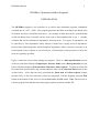
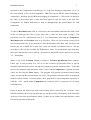
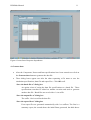
Figure 1 shows the screen when starting the program. There is a Data specifications section
at the top with three buttons (Components, Persons, Items) and a Data generation section
below with three buttons (Generate data, Show data, Show reports). To generate a data file
first enter data specifications (top section) and then click on the Generate data button in the
section below. After data has been generated the Show data and Show reports buttons
become active so the user can look at what was generated. End the program using the Exit
button at the bottom of the screen or choose Exit under the File menu. Note: The user has to
exit the program first and then start the program again to generate another file.
RUMMss Manual
3
Figure 1. RUMMss screen when starting the program.
1. Components
The first thing to do when generating a data file is to supply information in the Components
form.
•
On the main screen choose Components
•
On the Components form select the number of components
With number of components is meant number of subsets of items or number of
dimensions in the data. When simulating unidimensional data the number of
components = 1. To simulate multidimensional data (trait dependence) the
number of components > 1.
ƒ
If number of components = 1 then all items belong to the same set (no trait
dependence). This is the default.
ƒ
If number of components = 2 then dependence can be specified since there
are two components. Next specify the correlation between the components. It
RUMMss Manual
4
can be specified as the correlation coefficient r or the constant c where c = (1r)/r. (see appendix 1 for an explanation of the constant c)
ƒ
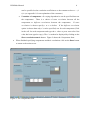
If number of components > 2 varying dependencies can be specified between
the components.
There is a choice of same correlation between all the
components or different correlations between the components.
If same
correlation is chosen specify r or c as before. If the different correlation
option is chosen then only c’s can be specified, one for each component (Click
in the cell for each component and type the c value or press enter after first
value has been typed to copy). The r’s can then be displayed by clicking on the
Show correlation matrix button. Figure 2 shows the Components form.
•
When finished specifying components and their correlations click on the Done button
to return to the main screen.
Figure 2. The Components form
RUMMss Manual
5
2. Persons
•
Now click on the Persons button on the main screen.
•
On the Persons form specify the following Person details:
Number of persons: Type in the number of persons to generate data for. The default
is 1000.
Rnd seed: If a random seed number is not entered the program picks a number to start
generating random person locations from. If entered by the user specify a number
between 0 and 32000.
Id Prefix: In the ID prefix box the user can type in alpha or numeric characters to
appear as part of a person ID in the generated data file. The rest of the ID is the
sequential number of the person generated.
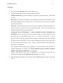
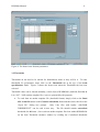
Component Person Distribution: A mean, standard deviation, minimum and
maximum value can be specified for the person locations in each component. If not
entered by the user the default values are 0, 2, -15 and 15 respectively. A set of
person locations will be generated with minimum, maximum, mean and standard
deviation values as specified. Click in each cell and type the value or press enter after
the first value has been typed to copy.
Figure 3 shows the Person form with values
entered for 3 components.
The common person location (β in appendix 1) can be written to the data file or
omitted depending on whether the Write simulated person location (common
ability) to the generated data file box is checked.
Persons with extreme scores can be included in or excluded from the data file
depending on whether the Exclude extreme scores box is checked.
•
When finished specifying Person details click on Done button to return to the main
screen.
RUMMss Manual
6
Figure 3. The Persons form
3. Items
•
Now click on the Items button on the main screen to specify the Items details. First
specify the Number of Items and then press ENTER. When enter is pressed the
number of lines in the Item specifications frame is adjusted so that there is one line for
each item. So each item has a line for its specifications.
•
Then specify the details for each item by selecting from the tabs called Natural
parameters,
Thresholds,
Discrimination,
Item
reversal
and
Response
Dependency. Not all these options have to be specified.
3.1 Natural parameters
The first specifications are the natural parameters of Maximum score, Location, Item unit,
Skewness, and Kurtosis for each item. Before that can be specified enter the Component
that the item belongs to in to the Components column, for example if 2 components were
RUMMss Manual
7
specified on the Components form then type a 1 if the item belongs to component 1 or a 2 if
the item belongs to the second component. NB. First specify all the items belonging to
component 1, and then specify all items belonging to component 2. Click in the cell and type
the value or press enter after a value has been typed to copy the value to the next line.
Components are shaded differently to help in distinguishing the specifications for each
component.
To enter a Maximum score click in a cell next to the item number and enter the value (Click
in the cell and type the value or press enter after a value has been typed to copy). The
maximum score for a dichotomous item is 1. For dichotomous items only the Component,
Maximum score and Location need to be specified. These are the minimum required item
specifications that have to be entered for each dichotomous item. Item unit, skewness and
kurtosis are not available for an item once a user has entered a maximum score of 1 for the
item, that is, they are not available for dichotomous items. For polytomous items Item unit,
Skewness and Kurtosis can be entered. Alternatively thresholds can be entered (see section
3.2 - Thresholds).
When a cell in the Location column is clicked a Location specification frame appears.
Either type in each location in a cell or use the Location specification frame to specify
minimum and maximum values, leaving the program to generate location values. To do that
specify the minimum and maximum values, select which Component to generate location
values for and click the Done button. The program will generate locations between those
values and specify the increment that was used. The generated location values are displayed
in the Location column. Location values can be generated for each component separately or
with the ‘ALL’ option under Component the locations will be generated for all items
simultaneously.
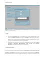
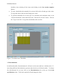
Figure 4 shows the Items form with some location values entered for the 15 items. Once
Natural parameters have been specified the user can proceed by selecting any of the other tabs
at the top of the Item specifications frame. If there are no further item specifications a data
file can be generated at this point.
RUMMss Manual
8
Figure 4. The Items form: Natural parameters
3.2 Thresholds
Thresholds do not need to be entered for dichotomous items as they will be 0. To enter
thresholds for polytomous items click on the Thresholds tab at the top of the Item
specifications frame. Figure 5 shows the Items form when the Thresholds tab has been
selected.
Threshold values can be entered manually, read in from a RUMM2020 (Andrich, Sheridan &
Luo, 1997 - 2005) anchor template file (*.anc) or generated by the program:
•
To read from an anchor template file (threshold format) simply click on the Read
ALL from file button on the Generate thresholds frame and then select the file at the
“Open file” dialog box prompt.
Only *.anc files with header “ANCHOR
THRESHCENT” can be read in this way.
The file should contain centralised
thresholds for all items. (Save such an anchor template file from within RUMM2020
on the Item Threshold estimates window by clicking the Centralised thresholds
RUMMss Manual
9
checkbox, then selecting all the items and clicking on the Save anchor template
button.)
•
To enter a threshold value manually for an item click in the cell and type in the value.
To copy that value to the next line simply press ‘enter’.
•
To generate thresholds for an item type in a minimum and maximum value in the
‘Generate thresholds’ frame and click on the ‘Generate for an item’ button. Click on
the ‘Copy to next line’ to copy those thresholds to the next line.
Figure 5. The Items form: Thresholds
3.3 Discrimination
In the Rasch models, discriminations for all items are the same and have a default value of 1.
Specifying different discriminations generates data that do not fit Rasch models. To change
the discrimination for an item click on the Discriminations tab at the top of the Item
specifications frame. Click in the required cell and change the value.
RUMMss Manual
10
3.4 Item reversal
Items in questionnaires (e.g. attitude questionnaires) sometimes need to be scored in reverse.
The Item Reversal option simulates this situation. Click on the Item reversal tab at top of
the Item specifications frame and double click in the cell for an item that has to be scored
negatively. An ‘R’ appears indicating that that item will be reverse scored. A double click in
the cell will change the ‘R’ back to a space.
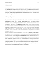
3.5 Response Dependence
To generate data with response dependence for certain items click on the Response
Dependence tab at the top of the Item specifications frame.
To simulate response
dependency specify, in the Dependent on Item column, which item that particular item is
dependent on. Then specify, in the Dependency Value column, by how much. For example,
if a person’s response to item 5 is dependent on their response to item 4 type 4 in the
Dependent on Item column for item 5 and type a value greater than 0 in the Dependency
Value column for item 5.
The greater the dependency value the greater the response
dependency. Figure 6 shows how to enter values so that item 5 is dependent on item 4 with a
dependency value of 2.
Response dependency is then simulated in one of two ways: a) changing the thresholds of
the dependent item so as to increase or decrease the probability of an identical response
(polytomous items), or b) changing the item difficulty of the dependent item so as to
increase or decrease the probability of a similar response (dichotomous and polytomous
items). With item 5 dependent on item 4 for example, whether the probability is increased or
decreased for item 5 depends on how the person scored on item 4. The default method
changes the thresholds. See Appendix 2 for further explanation of the simulation algorithm.
Note: The Component column here only indicates, as a guide to the user, which component an
item belongs to. The component values can not be changed here.
RUMMss Manual
11
Figure 6. Items form: Response dependence
4. Generate data
•
After the Component, Person and Item specifications have been entered now click on
the Generate data button to generate the data file.
•
Three dialog boxes appear one after the other requesting a file name to save the
simulation specifications, data file and report files. Click OK to all.
“Save the batch file as” dialog box
An option exists of saving the data file specifications to a batch file. These
specifications can then be edited on another occasion and used to generate
another data file. Batch files are saved with a *.sim suffix.
“Save the output file as” dialog box
The suffix *.dat is used for the data file.
“Save the report file as” dialog box
Four report files are generated automatically with *.txt suffixes: The first is a
summary report, the second shows the initial Betas generated, the third shows
RUMMss Manual
12
the A’s (see appendix), and the fourth shows the final Betas generated (see
Appendix 1 – simulation algorithm).
•
The program also generates automatically two RUMM2020 template files: the Data
Design template file (*.itm) and the Item Specification template file (*.spc). These
files will have the same name as the data file but with the suffixes .itm and .spc.
5. Data file and Reports
Click on the Show data and Show reports buttons to inspect the data and reports.
6. File menu
To read in a Batch file of simulation specifications:
•
From the File menu choose Batch
•
In the Open file dialog box select the name of the batch file that has to be opened and
click OK. The simulation specifications will appear in the respective Component,
Persons and Items forms.
RUMMss Manual
13
Appendix 1: A simulation algorithm for trait dependence
The algorithm for simulating trait dependence allows for different components in data, with
each component consisting of a set of items. The latent traits underlying the responses to
these components (respectively β1 , β 2 ,... etc.) can be correlated amongst each other to varying
degrees. The probability of a correct response on an item is thus increased or decreased
through a changed person ability β depending on the component.
Consider the case of an assessment with two components. Let B1 and B2 be the two latent
variables which are assessed by two sets of items, called components above. The latent
variable B1 is involved in responding to component 1 and the latent ability B2 is involved in
responding to component 2. B1 and B2 are correlated to varying degrees, sometimes
approaching 1. Let β, β1 and β2 be three other variables which are not correlated with each
other. Let β be the common component of B1 and B2, which is the source of the correlation
between them. Let β1 and β2 reflect the unique aspects of each of the components of items.
Let the distributions of β, β1 and β2 be identical, normally distributed with mean 0 and
standard deviation 1.
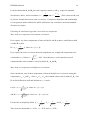
To construct a value for B1 and B2 for each person, the first step is to simulate three
independent standard normal random deviates β, β1 and β2.
Then define B1 = a1 +
b1
1+ c2
A1 and B2 = a 2 +
b2
1+ c2
A2
where A1 = β + c β1 and A2 = β + c β2
The source of the correlation between B1 and B2 is the common latent variable β; the source
of the correlation not being 1.0 is the presence of β1 and β2 with c>0. With c>0 independence
is violated because the correlation among item responses within a component is greater than
the correlation among items from different components (This is shown under Special:
correlation within a component).
RUMMss Manual
14
It can be shown that B1 and B2 have the respective means a1 and a2, respective standard
1
and c =
1 + c2
deviations b1 and b2, and a correlation r12=
2
1 − r12
. (This is shown in B1 and
r12
B
B2: Means, Standard deviations and correlation). Using these definitions and relationships
B
we can generate latent variables B1 and B2 which have any correlation, mean and standard
deviation we require.
Extending the simulation algorithm: more than two components
More than two components and common correlation
If we require, say, three components of items, define B1 and B2 as above, and define a third
variable B3 so that
B3 = a 3 +
B
b3
1+ c2
A3 where A3 = β + c β3
If we require the same correlation between components, for example all components to be
correlated at r = 0.6 then c =
1− r
= 0.82. Note that since r is the same between all
r
components the same constant c is used to define B1 , B2 and B3.
More than two components and different correlations
Now consider the case of three components of items with different correlations among the
components: r12, r13 and r23. Since r12 ≠ r13 ≠ r23 the constant values used to define B1, B 2 and
B3 will be different as well and defined as c1, c2 and c3.
B
Let B1 = a1 +
and B2 = a 2 +
b1
A1 where A1 = β + c1 β1
1+ c
2
1
b2
1+ c
2
2
A2 where A2 = β + c2 β2, etc.
For the sake of simplicity define E1 =
1
1+ c
2
1
, E2 =
1
1+ c
2
2
, and E3 =
Then it can be shown that r12 = E1E2, r13 = E1E3 and r23 = E2E3.
1
1 + c32
.
RUMMss Manual
15
In the case of three components of items the three correlations are independent of each other.
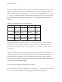
However, consider the case of four components that are all correlated differently with each
other. This results in six correlations (r12, r13, r14, r23, r24 and r34) that then define c1, c2, c3 and
c4. These six correlations can not be independent of each other and in the correlation matrix
there will be relationships among the correlations. The correlation matrix is defined as in
Table A1.
Table A1 Correlation matrix for four components
Component
1
2
3
4
R14
1
R11 =1
R12 =E1E2
R13 =E1E3
=E1E4
R24
2
R21 =E2E1
R22 =1
R23 =E2E3
=E2E4
R34
3
R31 =E3E1
R32 =E3E2
R33 =1
=E3E4
4
R41 =E4E1
R42 =E4E2
R43 =E4E3
R44 =1
Note that given all the four values of E (E1, E2, E3 and E4) in one row or one column of the
matrix the entire six correlation coefficients can be calculated. Thus six correlations are
generated from four latent variables, indicating that the six correlations cannot be entirely
independent.
Using this simulation rationale we can generate data sets with components of items that are
correlated according to a given correlation. In the case of more than two components the
traits underlying the components can be correlated equally or the traits can have different
correlations with each other, though when the number of components is greater than three, the
correlations are not totally independent.
B1 and B2: Means, Standard deviations and correlation
B
Let the correlation between the intermediate A1 and A 2 be r12 . It will be shown that this is
the same correlation as that between B1 and B2 when the latter are fully defined.
RUMMss Manual
16
cov[ A1 , A2 ]
Then r12 =
(A1)
V [ A1 ] V [ A2 ]
However, cov[A1,A 2 ] = cov[β + cβ1,β + cβ2 ] = cov[β,β] = V [ β ] . This follows because the
correlation among β , β1 , β 2 is mutually 0.
That is
cov[A1,A 2 ] = V [ β ] = 1.
(A2)
Now
V [ A1 ] = V [ β + cβ1 ] = V [ β ] + c 2V [ β 1 ]
(A3)
and
V [ A2 ] = V [ β + cβ 2 ] = V [ β ] + c 2V [ β 2 ]
(A4)
and this follows again because the correlation among β , β1 , β 2 is mutually 0.
Substituting (A2), (A3) and (A4) into (A1) gives
r12 =
V [β ]
V [ β ] + c 2V [ β1 ] V [ β ] + c 2V [ β 2 ]
(A5)
However, V [ β ] = V [ β1 ] = V [ β 2 ] =1.
Therefore, on simplifying (A5)
r12 =
and
c2 =
1
1 + c2
1 − r12
r12
(A6)
(A7)
RUMMss Manual
17
Clearly if c = 0, then r12 = 1, as it should be. The greater the value of c, the smaller the
correlation.
Thus any correlation between A1 and A 2 , (and therefore between B1 and B2 ), can be defined
in terms of c.
Now we define B1 and B2 :
Define B1 = a1 +
b1
1 + c2
A1
and B2 = a 2 +
b2
1 + c2
A2
Then the means of B1 and B2 are respectively a1 and a 2 ,
their variances are b12 and b 22 , and their intercorrelation is
r12 =
1
1 + c2
.
This is proved below. First note that
E[ A1 ]= E[ β + cβ1 ] =E[ β ]+ cE[ β1 ] = 0+ 0 =0 = E[A2 ]
and
V [ A1 ] = V [ β + cβ1 ] = V [ β ] + c 2V [ β 1 ] = 1+c2 = V [ A2 ] .
Then
E[ B1 ]=E[a1 +
b1
1 + c2
A1 ] = E[ a1 ]+ E[
b1
1 + c2
A1 ] = a1 +0 = a1 ,
and likewise E[ B2 ] = a 2 .
b12
b12
2
2
A1 ] =
V[ B1 ]=V[a1 +
2 V[ A1 ] =
2 (1 + c ) = b1
2
(1 + c )
(1 + c )
1+c
b1
and likewise, V[ B2 ] = b 22 .
(A8)
RUMMss Manual
18
Finally, COV[ B1 , B2 ] =
COV[ a1 +
= COV[
=
b1b2
1 + c2
b1
1 + c2
b1
1 + c2
b2
A1 ,
1 + c2
a2 +
b2
1 + c2
A2]
A2]
COV [ A1 , A 2 ]
bb
bb
= 1 22 (1) = 1 22
1+ c
1+c
Therefore,
A1 ,
(from A2: COV [ A1 , A 2 ] = V[ β ]=1).
COV[B1,B2 ]
bb
1
1
= 1 22
=
= r12 (from A6).
V[B1 ] V[B2 ]
1 + c b1b2 1 + c 2
Special: Correlation within a component
Consider the correlation among responses within component 1:
r11 =
cov[ A1 , A1 ]
V [ A1 ] V [ A1 ]
=
cov[ A1 , A1 ]
V [ A1 ]
COV[A1, A1] = COV[β+ c β1, β+ c β1]
= E[(β+ c β1)( β+ c β1)] – E[β+ c β1]E[β+ c β1]
= E[β 2 + c β1 β + c β1 β + c 2 β1 β1] – 0 * 0
= E[β 2 ] + c 2 E[β1 2 ]
= V[β] + c 2 V[β1]
and
V [ A1 ] = V [ β + cβ1 ] = V [ β ] + c 2V [ β 1 ]
then
r11 =
cov[ A1 , A1 ]
V [ A1 ] V [ A1 ]
=
V[ β ] + c 2V [ β 1 ]
=1
V [ β ] + c 2V [ β 1 ]
(A9)
RUMMss Manual
19
Appendix 2: Simulation algorithm for response dependence
Response dependence is simulated by making a person’s response on an item be a function of
the person’s response to a previous item. Specifically, response dependence is simulated by
making the probability of a person’s correct response on an item increase as a function of the
correct response, and decrease as a function of the incorrect response, on a previous item on
which it depends. How much the probability increased or decreases can be determined in two
ways:
a) Enhanced similar response: Simulating dependence is effected through changing the
difficulty δ by adding or subtracting a constant, d, from the difficulty of the dependent item,
or
b) Enhanced identical response: Simulating dependence is effected through changing the
difficulty δ , but indirectly through a constant d (or fractions of d) being added to or
subtracted from the thresholds (polytomous items only).
Simulation algorithm for an enhanced similar response
This algorithm describes how to simulate data for ordered categories and it specialises to the
dichotomous case.
Consider two items, item j dependent on item i. Let x nj ∈ {0,1,2...m j } be the integer response
variable for person n with ability β n responding to item j with difficulty δ j . τ 1 j ,τ 2 j ,...τ mj are
the thresholds between the graded responses and m j is the maximum score of item j. Let
x ni ∈ {0,1,2...mi } be the integer response variable for item i and mi the maximum score of that
item.
A person’s high score response on item i (higher than the middle category for the item or the
average of the scores of the two middle categories in case of an even number of categories)
increases the probability of a high score on the dependent item j and a low score on item i. A
RUMMss Manual
20
person’s low score response on item i (lower than the middle category for the item or the
average of the scores of the two middle categories in case of an even number of categories)
decreases the probability of a higher score on the dependent item j in the following way:
x
Pr{x nj | x ni } = [exp( x nj ( β n − δ j ) − (2( x ni − mi ) / mi + 1)d − ∑τ kj )] /
k =1
mj
∑ [exp( x
x =0
x
nj
( β n − δ j ) − (2( x ni − mi ) / mi + 1)d ) − ∑τ kj )]
(A10)
k =1
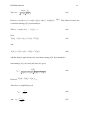
For example, consider item i with 5 categories, x nj ∈ {0,1,2,3,4} . For each value of xni
shown below β n − δ j − ( 2( x ni − mi ) / mi + 1)d works out to:
If xni = 0 then β n − δ j − (2(0-4)/4 + 1)d = β n − δ j − (-c) = β n − δ j + d
If xni = 1 then β n − δ j − (2(1-4)/4 + 1)d = β n − δ j − (-1/2c) = β n − δ j + 1/2d
If xni = 2 then β n − δ j − (2(2-4)/4 + 1)d = β n − δ j − (0) = β n − δ j
If xni = 3 then β n − δ j − (2(3-4)/4 + 1)d = β n − δ j − (1/2c) = β n − δ j -1/2 d
If xni = 4 then β n − δ j − (2(4-4)/4 + 1)d = β n − δ j − (c) = β n − δ j - d
Note that when xni = 0 then d will be added to δ j , decreasing the probability of a high
response on item j. When xni = mi then d will be subtracted from δ j , increasing the
probability of a high response on item j. d or fractions of d are added to or subtracted from
δ j depending on the distance of x ni from 0 or m i .
Simulation algorithm for an enhanced identical response
This algorithm affects the probability of a correct response on an item through changing the
thresholds ( τ 1 ,τ 2 ,...etc. ) of the item. To increase the likelihood of a response in the same
category for item j as item i the thresholds of the dependent item j are ‘moved’ in such a way
as to ‘enlarge’ that category by d.
Pr{x nj | x ni = mi } =
x
mj
x
k =1
x =0
k =1
[exp( x nj ( β n − δ j ) − ∑ (τ kj − d ))] / ∑ [exp( x nj ( β n − δ j ) − ∑ (τ kj − d )]
and
RUMMss Manual
21
Pr{x nj | x ni = 0 i } =
x
mj
x
k =1
x =0
k =1
[exp( x nj ( β n − δ j ) − ∑ (τ kj + d ))] / ∑ [exp( x nj ( β n − δ j ) − ∑ (τ kj + d )]
and
Pr{x nj | 0 < x ni < mi , x ni } =
xnj
⎫
⎧ xni
[exp( x nj ( β n − δ j ) − ∑ (τ kj − d / 2))] / ∑ [exp( x nj ( β n − δ j ) − ⎨∑ (τ kj − d / 2) + ∑ (τ kj + d / 2)⎬] )
k =1
xnj = 0
k = xni +1
⎭
⎩ k =1
x
mj
RUMMss Manual
22
References
Andrich, D. & Luo, G. (1997-2003). SimsRasch. RUMM Laboratory, Perth, Australia.
Andrich, D., Sheridan, B. & Luo, G. (1997-2005). RUMM2020. RUMM Laboratory, Perth,
Australia.