1
AgesGalore2
—
User and Reference Manual
Steffen Greilich
December 16, 2013
Contents
I
User Manual
3
1 Introduction
1.1 Summary . . . . . . . . . . . . . . . . . . . . . . . . . . . . . . .
1.2 History . . . . . . . . . . . . . . . . . . . . . . . . . . . . . . . .
4
4
4
2 Using AgesGalore
2.1 Installation . . . . . . . . . . . . . . .
2.2 Running the software . . . . . . . . . .
2.2.1 Interactive mode . . . . . . . .
2.2.2 Script mode . . . . . . . . . . .
2.2.3 Server mode . . . . . . . . . . .
2.3 General workflow with AgesGalore
7
7
7
7
8
8
9
.
.
.
.
.
.
.
.
.
.
.
.
.
.
.
.
.
.
.
.
.
.
.
.
.
.
.
.
.
.
.
.
.
.
.
.
.
.
.
.
.
.
.
.
.
.
.
.
.
.
.
.
.
.
.
.
.
.
.
.
.
.
.
.
.
.
.
.
.
.
.
.
.
.
.
.
.
.
.
.
.
.
.
.
.
.
.
.
.
.
3 List of commands
12
4 Detector models
17
4.1 General . . . . . . . . . . . . . . . . . . . . . . . . . . . . . . . . 17
4.2 Simple detector . . . . . . . . . . . . . . . . . . . . . . . . . . . . 18
5 Protocols
5.1 MASS
5.1.1
5.1.2
5.1.3
. . . . . . . . . . . . . . . . . .
Growth curve . . . . . . . . . .
Equivalent dose . . . . . . . . .
Recycling rations, fading rates
.
.
.
.
.
.
.
.
.
.
.
.
.
.
.
.
.
.
.
.
.
.
.
.
.
.
.
.
.
.
.
.
.
.
.
.
.
.
.
.
.
.
.
.
.
.
.
.
.
.
.
.
.
.
.
.
.
.
.
.
20
20
20
21
21
6 Fitting routines
22
6.1 Linear . . . . . . . . . . . . . . . . . . . . . . . . . . . . . . . . . 22
6.2 Exponential saturation . . . . . . . . . . . . . . . . . . . . . . . . 22
7 Grain segmentation
24
7.1 Using ImageJ . . . . . . . . . . . . . . . . . . . . . . . . . . . . 24
7.2 Using AgesGalore . . . . . . . . . . . . . . . . . . . . . . . . . 29
1
II
Reference Manual
8 Class description
8.1 Photon counts . . . .
8.2 Growth curve . . . . .
8.3 Dose reponse . . . . .
8.4 Evaluation . . . . . . .
8.4.1 Dose evaluation
8.5 Protocol . . . . . . . .
8.6 Detector . . . . . . . .
8.7 Data . . . . . . . . . .
30
.
.
.
.
.
.
.
.
.
.
.
.
.
.
.
.
.
.
.
.
.
.
.
.
.
.
.
.
.
.
.
.
.
.
.
.
.
.
.
.
9 Result format
.
.
.
.
.
.
.
.
.
.
.
.
.
.
.
.
.
.
.
.
.
.
.
.
.
.
.
.
.
.
.
.
.
.
.
.
.
.
.
.
.
.
.
.
.
.
.
.
.
.
.
.
.
.
.
.
.
.
.
.
.
.
.
.
.
.
.
.
.
.
.
.
.
.
.
.
.
.
.
.
.
.
.
.
.
.
.
.
.
.
.
.
.
.
.
.
.
.
.
.
.
.
.
.
.
.
.
.
.
.
.
.
.
.
.
.
.
.
.
.
.
.
.
.
.
.
.
.
.
.
.
.
.
.
.
.
.
.
.
.
.
.
.
.
.
.
.
.
.
.
.
.
31
31
31
31
31
31
31
31
31
32
2
Part I
User Manual
3
Chapter 1
Introduction
1.1
Summary
AgesGalore is a software designed to evaluate spatially resolved luminescence
data, especially in the frame-work of luminescence dating. It allows the user to
• display the raw signal data which are preferably obtained by CCD detectors.
• infer the actual photon counts from the raw signal data. For this purpose
it features a series of detector models, i.e. mathematical representations
of the photon-to-signal conversion processes in a (low light) detector (see
chapter 4).
• establish growth curves (dose responses) or shine-down curves (time dependencies) using the photon count data employing protocols that reflect
the measurement sequence (such as a single aliquot regeneration etc., see
chapter 5).
• use curve-fitting procedures (see chapter 6 to compute the equivalent or
paleo-dose(s) for the sample, both for each pixel of an image and predefined
regions of interest (ROIs).
• analyze the results in a way adapted for spatially resolved luminescence
data, i.e. using additional spatial filtering.
Please note, that these features were all covered by AgesGalore1 whereas
its successor AgesGalore2 is still not including all of them.
1.2
History
I started to write AgesGalore during my PhD thesis in order to analyze the
data from my OSL experiments. The software was at that time not intended
4
for general use and grew rather chaotically and driven by demand. AgesGalore was written in C++ using Microsoft Visual Studio 6.0 and ran on
Windows machines.
Before I left the lab, an ”official” version (1.0.0 as of May 8th, 2006) was
released to preserve the ability to analyze spatially resolved OSL data for future
in-house research and interested colleagues ([1]). At this time AgesGalore
was closed code. There was no actual license but users were asked to registered
and after sending the installation ID generated during installation they received
an unlock key that would allow to use all features of the software.
In 2012, with the advent of the CCD-equipped lexsyg reader ([2]) and
the need for a corresponding software, AgesGalore was considered to be a
promising candidate but had be made fit for reasonable use by commercial
users. Within approximately 100 man hours, the worst bugs were fixed, the
design improved and the code changed to compile using Visual Studio 2010
and to run on Windows 7. It became clear, however, that the design of the
software (C++/MFC with user-interface and functionality inseparable knotted)
was a dead end. The last version of AgesGalore was 1.10.1 (build 2 as of Aug
14th, 2012).
Consequently, AgesGalore2 was started in 2013 as a completely new software designed from scratch.
• By using Java as programming language, effective development and crossplattform compatibility could be assured. As both Java and C++ are
object-oriented languages, successful structures that reflect entities or processes in luminescence dating could be transferred directly.
• Java allowed to use the NIH-hosted software ImageJ (the public domain
gold standard for post-processing of microscopy data) as a class library.
Thus, AgesGalore2 could be freed from unnecessary code, e.g. for handling image data, regions of interest, I/O, which made the software and
its development leaner and faster.
• Additionally this approach allowed to access a plethora of ImageJ ”plugins”, e.g. for single grain segmentation, image processing etc.
• To provide a tiered structure, AgesGalore2 was designed as a shell, to
be controlled with text commands like data loadImage -file test.SPE.
This allows to implement graphical user interfaces without intermingling
with the functionality.
• AgesGalore2 was designed from the beginning to generically deal with
single grain and rock slice samples while its predecessor was mainly limited
to rock slices.
In the following document ”AgesGalore” always refers to AgesGalore2
if not stated otherwise.
5
Status
25. Oct 2013
S. Greilich
Started document
6
Chapter 2
Using AgesGalore
2.1
Installation
AgesGalore comes as a java archive file (extension .jar) that contains both its
own classes and third party classes needed (such as ImageJ). To run AgesGalore you have to have Java, version 7 or later, installed. AgesGalore runs on
all platforms that can run Java. You can download Java here: http://www.java.com.
2.2
2.2.1
Running the software
Interactive mode
To start AgesGalorein interactive mode, open a new terminal or command
line window and type:
java jar AgesGalore.jar
This will start the AgesGalore shell where you will be prompted to enter
commands (see chapter 3) and the software will respond immediately. To end
AgesGalore enter quit.
In case your are processing lage data sets, you might experience that the
Java Virtual Machine runs out of memory. Then, add an additional -Xms flag
in between java and -jar to increase the memory allocated for Java:
java -Xms6000m jar AgesGalore.jar
Here, 6 GB (6000 MB) are allocated. Of course, this only works if your PC
has a corresponding amount of RAM available.
7
2.2.2
Script mode
AgesGalore can also be run in script mode, i.e. driven by an external file.
To do so, open a new terminal or command line window and type:
java jar AgesGalore.jar Script.txt
where Script.txt is a plain text file containing AgesGalore commands,
with a single command per line, for example:
// This is a comment: TestScript for reading ImageSequence from lexsyg
data setWD -path Sor3_NGS0013
data loadImageSequence -file Sor3_NGS0013_DRT_r512.SPE \\
-sequence 11-NAT-11-TD-50;11-REG-50-11-TD-50;11-REG-100-11-TD-50;\\
11-REG-150-11-TD-50;11-REG-0-11-TD-50;11-REC-50-11-TD-50
rois load -file RoiSet.zip
detector set -type Simple -parameter 600
protocol set -type MASS -interval 1,2,8,10 -useTestDose
data list
eval dose -fitType Linear
data list
eval dose -fitType ExpSat
data list
eval save -index 1
eval save -index 2
exit
If the last command (exit) is skipped, AgesGalore will enter in interactive
mode. Script mode can facilitate the routine use of AgesGalore.
2.2.3
Server mode
AgesGaloredoes also support running as server. Commands can be send using
Port 9090 from a user client. To start AgesGalore in server mode, type:
java jar AgesGalore.jar server
The client can be a simple telnet program or more likely a custom made software. The following code is an example client that reads a script (Script.txt)
and sends it to AgesGalore line by line.
package agesgaloregui;
import
import
import
import
import
java.io.BufferedReader;
java.io.FileReader;
java.io.IOException;
java.io.InputStreamReader;
java.io.PrintWriter;
8
import java.net.Socket;
public class AgesGaloreGUI {
public static void main(String[]
Socket
socket
=
PrintWriter
out
=
BufferedReader in
=
args) throws IOException, InterruptedException {
null;
null;
null;
try{
socket = new Socket("localhost", 9090);
out
= new PrintWriter(socket.getOutputStream(), true);
in
= new BufferedReader(new InputStreamReader(socket.getInputStream()));
} catch (IOException e) {
System.err.println("Couldn’t get I/O for "
+ "the connection to AgesGalore server.");
System.exit(1);
}
FileReader
BufferedReader
String
scriptFile
inFile
line, read;
= new FileReader("Script.txt");
= new BufferedReader(scriptFile);
while((line = inFile.readLine()) != null){ // If line successfully read in
out.println(line);
System.out.println("GUI sent> " + line);
read = in.readLine();
System.out.println("GUI received> " + read);
}
out.close();
in.close();
inFile.close();
socket.close();
System.exit(0);
}
}
2.3
General workflow with AgesGalore
A typical workflow will look similar to the series of commands given as a script
example in 2.2.2. The commands and their structure are documented in chapter
3.
1. First of all, the user will point AgesGalore to a working directory where
9
(preferably) the original data is located and where the results will be
stored:
data setWD -path PathToDir
If the directory not exists, it will be created (given sufficient user right,
correct path name etc.).
2. Then the user will load images with the raw digital signal data individually
or in a sequence (standard for the lexsyg system) and attribute each
image or image series a dose group (i.e. natural signal, regenerated signal,
recovery signal, fading test signal, see chapter 5 on protocols for more
information) as well as a dose (if known, not needed for the natural signal )
and if applicable an image that represents the corresponding test dose
measurement. In this case, again, a dose value has be given, in the case
of course also for the test dose measurement of the natural signal, e.g.:
data loadImageSequence -file ImageFile -sequence ImageSequence
3. Most likely the user wants to evaluate the dose response for each pixel of
the images but also for regions of interest (ROIs). These include a number
of pixels and represent for example a single grain. To do so, users have to
load either an externally defined set (in zipped ImageJ format):
rois load -file ROIfile.zip
or trigger AgesGalore to start ImageJ plugins for the definition of
ROIs:
rois create
[NOT YET FUNCTIONAL!].
4. Then, the user has to chose which detector and which protocol they want
to use (detector set ..., protocol set .... The first will determine
the way in which the raw signal data are converted into estimated photons
counts (see chapter 4), the latter how these photo count data are used to
establish a growth curve / dose response (see chapter 5).
5. Using
data list
the user gets an overview on the data and results AgesGaloreholds in
its memory at the time of the execution.
6. The actual growth curve and equivalence dose computation is then started
using
10
eval dose -fitType XXX
where XXX is the fit to that should describe the relation between dose and
photon counts (see chapter 6). After the evaulation is done it appears in
the list when calling data list.
7. The user can then save any of the evaluations they did by
eval save -index i
to disc where it is stored in the working directory in the format described
in .
Status
25. Oct 2013
S. Greilich
Started document
11
Chapter 3
List of commands
Commands in AgesGalore are completely text based. They consist of a main
command that represents the area of application (data, rois, etc.), subcommands that refer to the actual action (loadImage, save) and – if applicable
– parameters, consisting of a keyword (starting with -̈¨) and a value. Parameters can be given in any order. If a command or subcommand is unknown or
a parameter is missing, AgesGalore will prompt the user accordingly. The
follwing table summarizes all commands available (at the moment) in AgesGalore.
12
Command
Subcommand
Parameters
Function
data
clear
none
removes all data
list
none
lists all data
sets working directory
setWD
-path
path of working directory, can be
relative (with respect to location
of AgesGalore2.jar) or absolute.
Will be created if does not exist.
loads an image (tif, png, jpg,
WinSpec, ...) and attributes it
to a dose group
loadImage
-file
-fileTestDose
-type
-dose
-testdose
file name
file name for test dose image (optional)
dose group type (NATural, REGenerated, RECycled, or FADingtest)
dose given to sample (in arbitrary units), not necessary for
NAT
test dose given to sample (a.u.)
loads an image (esp. WinSpec
from lexsyg system) containing
several (or all) steps of a measurement.
loadImageSequence
-file
-sequence
13
file name
sequence of the measurement,
syntax:
Number of images for step
- dose group type - dose
(where needed);
detector
set
sets the current detector model,
implemented at the moment:
1. SIMPLE, see 4.2
To check if a detector is set use
”data list”
-parameter
eval
dose
save
help
parameter for the chosen detector:
1. SIMPLE: a single number giving the background
performs a dose response evaluation, i.e. computes the equivalent dose, its error, for all ROIs
(if defined) and all pixels
-fitType
sets type of fit to be used implemented as at moment:
1. ”Linear”, see
2. ”ExpSat”, see
-index
saves the results of a dose evaluation to disk
displays this information.
14
protocol
rois
set protocol to use for doseresponse, implemented at the
moment:
1. MASS: SAR-like protocol for
pixelized data, see 5.1
To check if a protocol is set use
”data list”
set
-interval
Two or four numbers (will be
truncated to integer values) separated by ”,” that indicate the
(one-based) index of the time
intervals to integrate the signal and the background (see
5.1). For example, -interval
1,2,8,10 will integrate the first
two images of the shine-down
curve and subtract the 8. to the
10. image as background.
-useTestDose
If given, the photoncounts use
within the MASS protocol will be
normalized by the corresponding
testdose (Tx). For the testdose
signal, the integration rules given
using -interval apply as well.
loads ROIs (in ImageJ format,
zip)
load
-file
saveSignals
filename
saves average raw signal within
defined ROIs to .xml output file.
These data can be used in other
single grain evaluation tool, e.g.
after import by the corresponding function of the AgesGalore
R-package.
Status
15
25. Oct 2013
4. Nov 2013
16. Dec 2013
S. Greilich
S. Greilich
S. Greilich
Started document
Added new syntax for eval dose
Added saveSignals subcommand for ROIs
16
Chapter 4
Detector models
4.1
General
Detectors for luminescence measurements (in the real world) convert impinging
photons into a measurable signal. For the detection of light there is a large variety of detectors such as photomultiplier tubes (PMTs), Silicon photomultipliers
(Si-PMTs), (avalanche) photodiodes, or charge-coupled devices (CCDs). Each
detector comes with its own mechanism and hence properties for the conversion.
Among the parameters describing this conversion are:
• the quantum efficiency, i.e. the average probability to convert a photon.
• the background — the base signal that is measured in the absence (or
additionally) to the photon signal.
• various kind of noise that is created during the conversion or due to the
random arrival of photons.
• etc.
A detector in AgesGalore is a set of functions f that tries to mimic the
properties of a real detector and thus to infer the actual number of photons λ and
the uncertainty ∆λ that impinged on the detector from the raw digital signal z̃
that has been recorded and optionally other parameters. In this document we
follow the nomenclature used in [1]):
λ = fexp (z̃, ...)
(4.1)
∆λ = fvar (z̃, ...)
(4.2)
The computation of photon counts from signal data always happens before
AgesGalore uses the data, e.g. to evaluate the dose response of a sample.
Usually, the raw signal data are recorded in a number of time intervals ti .
In conventional luminescence dating these are often referred to as channels, in
17
AgesGalore they correspond to a series of images taked during the shine-down
of the sample. z̃ can therefore be obtained from a single or multiple subsequent
time intervals / channels / images by simply summing up the raw signal data
before the conversion to photon counts:
X
z̃ = z̃j1 ,j2 =
z̃(tj )
(4.3)
j=j1 ...j2
If not stated otherwise, z̃ will in the following always refer to the raw signal
data from either a single or multiple images. In contrast, z̃1,3 for example explicitly says that the raw signal data were summed from image 1 to 3.
In order to make photon counts from different time spans comparable, they
have to be converted into count-rates:
Λ(z̃j1 ,j2 ) =
fexp (z̃j1 ,j2 , ...)
λ(z̃j1 ,j2 )
=
(j2 − j1 + 1)
(j2 − j1 + 1)
(4.4)
This operation assumes a constant time of exposure for all images / channels
which might not be always the case. So, for future releases of AgesGalore2
the actual time span might be used rather than the indices – this would also
yields true rates.
For further information on photon counts and how arithmetic operations are
done on photon count data by AgesGalore, see section 8.1.
At the moment the following detectors are implemented in AgesGalore:
4.2
Simple detector
This detector assumes random, Poisson-governed arrival of photons and detection with perfect quantum efficiency. Additionally the detector has a (spatially
and temporally) constant background that can simply be subtracted. Thus, if z̃
is the observed digital signal, the expectation value of the photon counts λ can
be derived via
λ = fexp (z̃, ξ) = z̃ − ξ
(4.5)
where ξ is the (DC) offset, derived for example from a measurement with a
closed shutter. The uncertainty is given by
p
√
∆λ = fvar (z̃, ξ) = z̃ − ξ = λ
(4.6)
The simple detector is a good approximation for efficient detectors (high
quantum efficiency) at reasonable high photon count rates. When the count
rate is low, shortcomings become obvious, first of all the generation of negative
photon counts ([1]).
In cases where the MASS protocol (see section 5.1) subtract a later part of
the shine-down curve from an earlier to obtain Lx , ξ might be irrelavant.
18
Status
25. Oct 2013
4. Nov 2013
S. Greilich
S. Greilich
Started document
Added rates
19
Chapter 5
Protocols
Protocols determine how photon count data are used to establish a dose response
(growth curve). Up to now, the following protocols are implemented:
5.1
5.1.1
MASS
Growth curve
MASS is an extension of the well-known SAR protocol (single aliquot regeneration) to multi-pixel images, assuming that each pixel represents its own independent source of light and dose/age information, respectively. Thus, MASS
performs a SAR protocol on each pixel (yielding new images of spatial equivalent dose distribution, goodness of fit etc.) and on groups of pixels that have
been binned on the level of the raw signal data, i.e. regions of interest (ROIs,
e.g. for single grains)1 .
MASS use the photon count rates from multiple (n > 1) regeneration measurements
Λreg (Di , z̃j1 ,j2 )
(5.1)
where Di are the regeneration doses (with i = 1...n) and j1 and j2 the indices
of the first and the last subsequent image (channel) the raw signal was summed
over. Some Di can have the same value but not all of them. j1 and j2 have
to be the same for all Di . Thus, the simplest way to obtain the entries for the
growth curve LX is
LX (Di ) = Λreg (Di , z̃j1 ,j2 )
(5.2)
1 This means especially that the summed ROI raw signal data are converted into photon
counts and then used to establish a growth curve. This is an important difference between
AgesGalore 1 and AgesGalore 2. With the first, MASS computed equivalent doses for
each pixel first and THEN binned/averaged them to a ROI equivalent dose. This is a minute
but important difference.
20
where j1 will usually be 1 and j2 ≥ j1 has to be fulfilled.
More often, the a ”background signal”, obtained from later channels / images
in the shine-down curve will be used in addition, so that LX becomes:
LX (Di ) = Λreg (Di , z̃j1 ,j2 ) − Λreg (Di , z̃j3 ,j4 )
(5.3)
test
, z̃) exist
with j4 ≥ j3 > j2 . If the corresponding test dose data Λtest
reg (Di
and the user requested it, MASS can use the very same procedure for TX :
test
TX (Di ) = Λtest
reg (Di , z̃j1 ,j2 ) − Λreg (Di , z̃j3 ,j4 )
(5.4)
In this case, LX /TX is then used to establish the growth curve. In this case,
of course, all Ditest have to be the same.
5.1.2
Equivalent dose
To compute the equivalent dose Deq , AgesGalore performs curve-fitting to
the LX /TX (Di ) values using a function ffit (D, pi ) that depends on dose and a
set of parameters pi (see chapter 6). When the best set of parameters p̂i is
found, the natural signal is computed in the very same way as LX according to
Eq. 5.2:
LX (Deq ) = Λnat (Deq , tj )
(5.5)
or Eqs. 5.3, 5.4, resp. Then Deq can be found using the reverse of ffit
Deq = f −1 (LX (Deq ), p̂i )
(5.6)
The error of Deq , ∆Deq computed by Gaussian error propagation from the
∆Λ’s of all Λ’s involved.
5.1.3
Recycling rations, fading rates
Should be computed according to Eqs. 5.2 and 5.4, BUT ARE NOT IMPLEMENTED YET.
Status
25. Oct 2013
4. Nov 2013
S. Greilich
S. Greilich
Started document
Added rates
21
Chapter 6
Fitting routines
Fits are parametrized, analytical functions ffit (X, pi ) that are applied to find
hypothetical relation behind data. The depend on a variable X, e.g. dose
D or time t. For example, the dose response of a sample can be interpreted
as a straight line or as an exponential saturation. The user has the freedom
to chose (and always has to chose) the model they think is most appropriate.
AgesGaloreuses fits for example to compute the equivalent dose from a growth
curve which always has a limited number of data points only (see section 5.1.2).
To compare the growth curve to the natural signal and infer the equivalent dose,
the growth curve data have to be interpolated. This is in most cases best done by
fitting one of the following functions to the data point. The set of parameters
for which the ffit describes the data best is found in AgesGaloreusing the
minimization of the squared sum of the residuals.
6.1
Linear
The is a simple straight line with slope p1 and offset p2 .
y = p1 · x + p2
6.2
(6.1)
Exponential saturation
Starting from an offset for x = 0, this function approaches it upper limit exponentially. The approach is determined by the parameter p2 :
y = p1 · (1 − e−x/p2 ) + p3
(6.2)
For growth curves more often another nomenclature of this equation is used:
S = Smax · (1 − e−D/D0 ) + Sres
22
(6.3)
where the increase from a residual signal Sres at dose D = 0 to Smax at
D = ∞ is governed by the parameter D0 in units of dose. The two versions are
of course fully equivalent.
23
Chapter 7
Grain segmentation
For single grain evaluation, the user has to define regions of interest (ROIs)
which correspond to what is considered to be a grain. Within these ROIs, the
signal from all pixels will be summed and the grain thus be treated as one
entity. AgesGalore2 uses the ImageJ ROI format, which consists of binary
files – one for each ROI – with extension .roi. In the common case of multiple
ROIs, the binary files will be enclosed in a single, compressed file with extension
zip. The detection of grains and definition of ROIs is essentially an image
segmentation problem. Since a plethora of segmentation algorithms exists for
ImageJ, AgesGalore uses indirectly or directly (not yet) the corresponding
ImageJ plug-ins for maximum flexibility.
7.1
Using ImageJ
The use of ImageJ for segmentation is reasonable as long no ROI definition
from within AgesGalore is possible or if new algorithms should be tested.
The following describes the corresponding workflow.
1. First, download the latest version of ImageJ (version 1.x, not 2.x!) here:
http://rsbweb.nih.gov/ij/download.html. We recommend the version bundled with Java to avoid additional installation problems.
2. Install ImageJ on your machine.
3. To read images from a CCD camera in WinSpec format (extension .spe),
you need the SPE-plugin which is found here: http://rsbweb.nih.gov/
ij/plugins/spe.html. Follow the installation instructions on the page
(i.e. copy the files in your ImageJ plug-in directory and restart the program).
4. In this example, we use for segmentation an adaptive threshold algorithm
which is found here: https://sites.google.com/site/qingzongtseng/
24
Figure 7.1: Loaded CCD image in ImageJ and adjustment of brightness and
contrast.
adaptivethreshold. Download the version for your operating system
(Windows 32/64 bit, Linux etc.) and install following the instructions.
The page also features a description on how to use the plug-in.
5. Now, restart ImageJ and read in your image(s). Assuming the sample
has not been shifted, you can use any frame / image for segmentation,
preferably one with bright signal. For better contrast, use the adjustment
in ImageJ (Menu Image > Adjust > Brightness/Contrast, Fig. 7.1).
6. Convert your image to 8-bit format by choosing Image > Type > 8-bit.
7. Start the plug-in by choosing Plugins > adaptiveThr. A new dialog
(”Adaptive Threshold”, Fig. 7.2) will open. Check both ”Preview” and
25
Figure 7.2: Adaptive threshold user dialog.
”Output Mask?” and set the values so that grains are reasonably represented (highlighted in red). Irregularities and artifacts (e.g. small highlighted areas outside the grains, single highlighted pixels) can be adjusted
in a later step.
8. Click ”OK”. If asked whether to process all N images, answer no – we
only need the first one. This will create a new black/white image, called
the ”mask” (Fig. 7.3).
9. To transform the mask into ROIs, choose Analyze > Analyze Particles...,
which will open the dialog shown in Fig. 7.4. Be sure to check Add to
Manager and set Show to Overlay Outlines. Use the other settings at
your convenience (e.g. to get some statistics on the ROIs). Adjust the
fields Size and Circularity to fine-tune the segmentation. For example,
choosing Size = 0-Infinity will result in too many small ROIs (Fig.
7.5), while a setting like Size = 10-Infinity will yield the result seen
in Fig. 7.6, i.e. 23 ROIs corresponding to grains (the very dim ones were
not caught).
10. At the same time, the ROI Manager window (Fig. 7.7) will open and
display the ROIs. In this window, choose More > Save... to save the
26
Figure 7.3: Mask
Figure 7.4: Mask
27
Figure 7.5: Due to inproper settings for the Particle Analyzer, too many artifacts
were defined as ROIs that does not correspond to actual grains.
Figure 7.6: Useful ROI definition.
28
Figure 7.7: ROI Manager
ROI definitions as a file. Use a reasonable file name (e.g. your sample ID)
as you will have to later enter it into AgesGalore.
When using another plug-in for segmentation, steps 6, and 8-10 will be the
same.
7.2
Using AgesGalore
The definition of ROIs from within AgesGalore is not implemented yet.
Status
16. Oct 2013
S. Greilich
Started document
29
Part II
Reference Manual
30
Chapter 8
Class description
8.1
Photon counts
8.2
Growth curve
8.3
Dose reponse
8.4
Evaluation
8.4.1
Dose evaluation
8.5
Protocol
8.6
Detector
8.7
Data
Status
25. Oct 2013
S. Greilich
Started document
31
Chapter 9
Result format
Results are stored in the working directory within a uniquely named folder
(including a time stamp, the protocol used etc.). Within this folder the resulting
images (from MASS) are stored in 32bit-TIFF format. Additionally, an xml file
containing the information on the growth curve, the doses, the equivalent doses,
the fit parameters etc is saved. For the ROIs (if requested) the data is directly
in the xml file while for the image only links to the local image are given to
limit the size of the xml file.
Status
25. Oct 2013
S. Greilich
Started document
32
Bibliography
[1] Steffen Greilich, H.-L. Harney, Clemens Woda, and Günther A. Wagner.
AgesGaloreA software program for evaluating spatially resolved luminescence data. Radiation Measurements, 41(6):726–735, July 2006.
[2] Daniel Richter, Andreas Richter, and Kay Dornich. lexsyga new system for
luminescence research. Geochronometria, pages 1–9, 2013.
33