Download Master`s degree thesis

Master’s degree thesis
IP501909 MSc thesis, discipline oriented master
A Generic Modelling Approach for Heavy Lifting Marine
Operation
Jiafeng Xu
Number of pages including this page: 67
Aalesund, 05.27.2014
Mandatory statement
Each student is responsible for complying with rules and regulations that relate to
examinations and to academic work in general. The purpose of the mandatory statement is
to make students aware of their responsibility and the consequences of cheating. Failure
to complete the statement does not excuse students from their responsibility.
Please complete the mandatory statement by placing a mark in each box for statements 1-6
below.
1. I/we herby declare that my/our paper/assignment is my/our own
work, and that I/we have not used other sources or received
other help than is mentioned in the paper/assignment.
2. I/we herby declare that this paper
1. Has not been used in any other exam at another
department/university/university college
Mark each
box:
1.
2. Is not referring to the work of others without
acknowledgement
2.
3. Is not referring to my/our previous work without
acknowledgement
3.
4. Has acknowledged all sources of literature in the text and in
the list of references
4.
5. Is not a copy, duplicate or transcript of other work
5.
I am/we are aware that any breach of the above will be
considered as cheating, and may result in annulment of the
3. examination and exclusion from all universities and university
colleges in Norway for up to one year, according to the Act
relating to Norwegian Universities and University Colleges,
section 4-7 and 4-8 and Examination regulations paragraph 30.
4. I am/we are aware that all papers/assignments may be checked
for plagiarism by a software assisted plagiarism check
5. I am/we are aware that Aalesund University college will handle
all cases of suspected cheating according to prevailing guidelines.
6. I/we are aware of the University College’s rules and regulation
for using sources paragraph 29.
Publication agreement
ECTS credits: 30
Supervisor: Karl Henning Halse
Agreement on electronic publication of master thesis
Author(s) have copyright to the thesis, including the exclusive right to publish the document (The
Copyright Act §2).
All theses fulfilling the requirements will be registered and published in Brage HiÅ, with the approval
of the author(s).
Theses with a confidentiality agreement will not be published.
I/we hereby give Aalesund University College the right to, free of
charge, make the thesis available for electronic publication:
yes
no
Is there an agreement of confidentiality?
yes
no
yes
no
(A supplementary confidentiality agreement must be filled in)
- If yes: Can the thesis be online published when the
period of confidentiality is expired?
Date: 05.27.2014
ASSIGNMENT
MASTER THESIS 2014
FOR
STUD.TECHN. JIAFENG XU
A Generic Modelling Approach for Heavy Lifting Marine Operation
Background
Vessel-crane simulation has always been a helpful tool for marine operation training, operation
planning and product designing. Most designing works of crane and vessel require simulation results
of their hydrodynamic behaviour, while most simulations so far regard crane and vessel isolated,
without physical interaction with each other: the vessel always stays on its weight distribution
equilibrium and the crane always experiences a given vessel motion no matter changes on loaded
weight and operating posture. This issue often lowers the final performance of AHC (Active Heave
Compensation) and ballast water control, hence worse positioning of the submerged load.
Objective
Research Study
 Lagrangian physics
 Maritime Guidance, Navigation and Control theory
 Specification rules
 Vibration dynamics
 20SIM Modeling and programing skills
 CFD
Work
 Dynamic modelling of vessel, crane, cable, load and other appurtenance.
 Implementation of AHC control, joystick control
 Load hydrodynamics correlation analysis
 Integration of all sub-models
 Simulation test for different vessel, crane parameters
 Result analysis
The thesis should be written as a research report with summary, conclusion, literature references,
table of contents, etc. During preparation of the text, the candidate should make efforts to create a well
arranged and well written report. To ease the evaluation of the thesis, it is important to cross-reference
text, tables and figures. For evaluation of the work a thorough discussion of results is needed.
Discussion of research method, validation and generalization of results is also appreciated.
In addition to the thesis, a research paper for publication shall be prepared.
Three weeks after start of the thesis work, a pre-study have to be delivered. The pre-study have to
include:
 Research method to be used
 Literature and sources to be studied
 A list of work tasks to be performed
 An A3 sheet illustrating the work to be handed in.
A template for the A3 sheet is available on the Fronter website under MSc-thesis. This sheet should
also be updated when the Master’s thesis is submitted.
1
The thesis shall be submitted as two paper versions. One electronic version is also requested on a CD
or a DVD, preferably as a pdf-file.
Supervision at Aalesund University College: Karl H. Halse,
Karl H. Halse
Program coordinator
Jiafeng Xu
Stud. Techn.
Delivery: 30-05-2014
2
PREFACE
This thesis is submitted in partial requirements for a Master’s Degree in Ship Design for the auther. It
contains work done from January to May 2014 at Aalesund University College. The supervisor of on
the project has been Associate Professor Karl Henning Hals, Faculty of Maritime Technology and
Operations (AMO). The thesis has been made solely by the auther; some contents used in the project,
however, is based on previous works of others. Thorough reference has been made accordingly.
The thesis project is part of the ongoing research in the Ship Operation Lab at Aalesund University
College, whose activities support the ongoing development of the activities at the Offshore Simulator
Centre (OSC). The research outline was introduced in one of the previous papers Lifting Operations
for Subsea Installations Using Small Construction Vessels and Active Heave Compensation Systems
– A Simulation Approach from Ship Operation Lab. The target is to develop generic modelling method
for maritime simulation as a platform for both training and design purpose. The thesis project is also
an upgrading of my earlier model developed in the summer of 2013.
The project is an interdisciplinary task requiring different aspects of knowledge. One of the biggest
challenge in the research development is to integrate sub-systems from various sources into one
compatiable system. This is also the keypoint for the standardization and expansion of a generic
modelling method. I would like to thank my supervisor Associate Professor Karl Henning Halse for his
guidance and support throughout the entire thesis composition. The new ideas inspired and new fields
of knowledge introduced by him has always been fruitful to me.
I would also like to thank Associate Professor Vilmar Ærøy for his assistance on 20-sim modelling and
project ideas. I enjoy his teaching very much.
The gratitude also goes to Yingguang Chu for his crane model and assistance on 3D Mechanics
modelling. The project is far from over and I am looking forward to our cooperation in the future.
Finally, the thesis is also to commemorate my amazing two years in Norway.
Aalesund University College
May. 2014
Jiafeng Xu
3
ABSTRACT
This thesis project introduced a generic modelling approach for heavy lifting marine operation based
on 20-sim simulation and Matlab control. The model is a multi-body dynamic system which can be
divided into vessel, crane, cable, load, and control system. Physical entities are modelled either in
bond graph or directly using 3D Mechanics toolbox and connected by interactive power port. All
control scheme is modelled as signal flow separated from physical entities. The vessel is modelled as
6-DOF bond graph using parameters from SHIPX data, then connected to the crane model inside 3D
Mechanics unit. Crane model is controlled by outside manual/auto control scheme. Cable and load are
modelled inside 3D Mechanics with hydrodynamic behaviour represented by actuators. The
performance of each system is evaluated respectively by regulations and analysis. The simulation
examples of different combinations of sub-systems are given at the end. The project is aiming at
developing a generic modelling method serves as a multi-user training and design platform.
Standardization and potential for upgrading are to be expected in the future.
Keywords: generic modelling, simulation, vessel-crane interaction, hydrodynamics, 20-sim.
4
CONTENTS
ASSIGNMENT ......................................................................................................................................... 1
PREFACE................................................................................................................................................ 3
ABSTRACT ............................................................................................................................................. 4
CONTENTS ............................................................................................................................................. 5
LIST OF FIGURES .................................................................................................................................. 7
LIST OF TABLES ................................................................................................................................... 8
TERMINOLOGY ...................................................................................................................................... 9
1
INTRODUCTION ............................................................................................................................ 10
1.1
1.2
1.3
1.4
1.5
2
BACKGROUND ........................................................................................................................... 10
MOTIVATION AND OBJECTIVE ..................................................................................................... 10
ORGANIZATION OF THESIS ......................................................................................................... 11
METHODOLOGY ......................................................................................................................... 11
LITERATURE AND PREVIOUS W ORK ............................................................................................ 12
MULTI-BODY DYNAMICS ............................................................................................................ 13
2.1
LAGRANIAN MECHANICS ............................................................................................................ 13
2.1.1
Lagrange Equations of the Second Kind ......................................................................... 13
2.1.2
Kirchhoff Equations .......................................................................................................... 13
2.2
BOND GRAPH MODELLING ......................................................................................................... 14
2.2.1
Standard Bond Graph Modelling ..................................................................................... 14
2.2.2
Modified Bond Graph Modelling ...................................................................................... 14
2.2.3
20-sim and 3D Mechanics Toolbox ................................................................................. 14
3
VESSEL MODEL ........................................................................................................................... 17
3.1
REFERENCE FRAMES................................................................................................................. 17
3.1.1
Reference Frame in ShipX .............................................................................................. 17
3.1.2
Reference Frame in 20-sim ............................................................................................. 17
3.2
MOTION EQUATION .................................................................................................................... 18
3.2.1
Equation of Vessel Hydrodynamics ................................................................................. 18
3.2.2
Coordinate Transformation .............................................................................................. 19
3.3
BOND GRAPH MODEL ................................................................................................................ 20
3.4
PARAMETERS ............................................................................................................................ 22
3.4.1
Calculation in ShipX ......................................................................................................... 22
3.4.2
MSS Post-process ........................................................................................................... 23
3.4.3
20-sim Parameter Input ................................................................................................... 23
3.5
MODEL ASSESSMENT ................................................................................................................ 24
3.5.1
Results ............................................................................................................................. 24
3.5.2
Discussion........................................................................................................................ 26
4
CRANE MODEL............................................................................................................................. 27
4.1
DYNAMIC SYSTEM ..................................................................................................................... 27
4.1.1
Solidworks Modelling ....................................................................................................... 27
4.1.2
Converting Steps and Tips .............................................................................................. 28
4.2
HYDRAULIC SYSTEM .................................................................................................................. 28
4.2.1
Main Derrick Sketch ......................................................................................................... 29
4.2.2
20-sim Modelling .............................................................................................................. 29
4.3
CONTROL SYSTEM .................................................................................................................... 30
4.3.1
Manual Control................................................................................................................. 30
4.3.2
Auto Control ..................................................................................................................... 31
5
CABLE MODEL ............................................................................................................................. 32
5.1
5.2
CABLE CHARACTERISTICS.......................................................................................................... 32
CATEGORIES OF CABLE MODEL ................................................................................................. 32
5
5.2.1
Method of Characteristics ................................................................................................ 32
5.2.2
Finite Element Methods ................................................................................................... 33
5.2.3
Linearization Method ....................................................................................................... 34
5.3
CABLE MODEL IN 3D MECHANICS............................................................................................... 34
6
LOAD MODEL ............................................................................................................................... 37
6.1
LIFTING OPERATION .................................................................................................................. 37
6.2
LOAD CFD ................................................................................................................................ 37
6.2.1
Motion Function of the Load ............................................................................................ 37
6.2.2
Velocity & Acceleration Dependent Coefficient ............................................................... 38
6.3
20-SIM MODELLING ................................................................................................................... 38
6.4
MODEL ASSESSMENT ................................................................................................................ 41
6.4.1
DNV Rules Calculation .................................................................................................... 41
6.4.2
FEM in 3D Mechanics ...................................................................................................... 42
6.4.3
Cable Parameters ............................................................................................................ 42
6.4.4
Results ............................................................................................................................. 43
6.4.5
Discussion........................................................................................................................ 47
7
SIMULATION EXAMPLE .............................................................................................................. 49
7.1
VESSEL + CRANE ...................................................................................................................... 49
7.1.1
Model ............................................................................................................................... 49
7.1.2
Results ............................................................................................................................. 50
7.1.3
Discussion........................................................................................................................ 52
7.2
VESSEL + CRANE + CABLE + LOAD ............................................................................................ 52
7.2.1
Model ............................................................................................................................... 52
7.2.2
Results ............................................................................................................................. 54
7.2.3
Discussion........................................................................................................................ 55
7.3
VESSEL + CRANE + CABLE + LOAD + AHC ................................................................................. 56
7.3.1
Model ............................................................................................................................... 56
7.3.2
Results ............................................................................................................................. 56
7.3.3
Discussion........................................................................................................................ 58
8
CONCLUSION & FUTURE WORK ............................................................................................... 59
8.1
8.2
CONCLUSION ............................................................................................................................ 59
FUTURE W ORK.......................................................................................................................... 59
REFERENCES ...................................................................................................................................... 60
APPENDIX ............................................................................................................................................ 61
APPENDIX A
APPENDIX B
APPENDIX C
APPENDIX D
APPENDIX E
USER MANUAL ........................................................................................................... 61
MATLAB SCRIPTS ....................................................................................................... 62
20-SIM MODELS (DIGITAL) ........................................................................................... 64
VIDEO FOOTAGE OF SIMULATION (DIGITAL) ................................................................... 64
20-SIM SCRIPTING LIBRARY ......................................................................................... 64
6
LIST OF FIGURES
FIGURE 1.1 W ORLD CONSUMPTION (MILLIONS TONNES OIL EQUIVALENT) (BP 2013) .................................. 10
FIGURE 2.1 20-SIM PANEL........................................................................................................................ 15
FIGURE 2.2 3D MECHANICS PANEL........................................................................................................... 15
FIGURE 3.1 BODY-FIXED REFERENCE IN SHIPX AND 20-SIM (T=T1) ............................................................ 18
FIGURE 3.2 BOND GRAPH OF SIMPLE VESSEL ........................................................................................... 20
FIGURE 3.3 VESSEL MODEL IN 3D MECHANICS ......................................................................................... 21
FIGURE 3.4 ACTUATOR IN 3D MECHANICS TOOLBOX ................................................................................. 22
FIGURE 3.5 USER PANEL FROM *.MAT FILE TO RUNNING 20-SIM MODEL ....................................................... 23
FIGURE 3.6 PARAMETERS PROCESS FROM SHIPX TO 20-SIM ..................................................................... 24
FIGURE 3.7 MOTION RAO FROM 20-SIM ................................................................................................... 25
FIGURE 3.8 MOTION RAO FROM SHIPX .................................................................................................... 25
FIGURE 3.9 ERROR BETWEEN 20-SIM AND SHIPX ...................................................................................... 26
FIGURE 4.1 SOLIDWORKS MODEL OF SIMPLIFIED ROLLS-ROYCE PSV-100 .................................................. 27
FIGURE 4.2 STEPS FROM SOLIDWORKS TO 20-SIM .................................................................................... 28
FIGURE 4.3 CRANE MODEL IN 3D MECHANICS .......................................................................................... 28
FIGURE 4.4 SIMPLIFIED MAIN DERRICK HYDRAULIC SKETCH ...................................................................... 29
FIGURE 4.5 BOOM CYLINDER HYDRAULICS MODEL .................................................................................... 29
FIGURE 4.6 BOOM CYLINDER SETUP IN 3D MECHANICS............................................................................. 30
FIGURE 4.7 CRANE TIP VELOCITY CONTROL ............................................................................................. 31
FIGURE 4.8 DIRECT CYLINDER VELOCITY CONTROL .................................................................................. 31
FIGURE 4.9 CYLINDER VELOCITY INPUT AND PID CONTROL ....................................................................... 31
FIGURE 4.10 COMPENSATING MOTION/VELOCITY ON OPPOSITE DIRECTION ................................................ 31
FIGURE 5.1 FOUR TYPES OF FEM CABLE MODEL...................................................................................... 33
FIGURE 5.2 FEM CABLE MODEL IN 3D MECHANICS ................................................................................... 34
FIGURE 5.3 EXTERNAL FORCE ACTING AS ACTUATOR ............................................................................... 35
FIGURE 5.4 CABLE MODEL (N=3, L=10) .................................................................................................... 35
FIGURE 5.5 EXTERNAL FORCE INPUT ........................................................................................................ 36
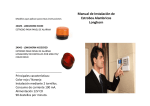
FIGURE 6.1 CFD EXPERIMENT TO TEST & VERIFY VELOCITY-ACCELERATION DEPENDENT COEFFICIENT ..... 38
FIGURE 6.2 LOAD MODEL IN 3D MECHANICS ............................................................................................. 38
FIGURE 6.3 BUOYANCY FORCE ACTUATOR ............................................................................................... 39
FIGURE 6.4 ADDED MASS AND DAMPING FORCE ACTUATOR ...................................................................... 40
FIGURE 6.5 CABLE + LOAD MODEL ........................................................................................................... 41
FIGURE 6.6 HORIZONTAL OFFSET WITH CURRENT FORCE ON LOAD V=1M/S ............................................... 43
FIGURE 6.7 HORIZONTAL OFFSET WITH CURRENT FORCE ON LOAD V=2M/S ............................................... 44
FIGURE 6.8 HORIZONTAL OFFSET WITH CURRENT FORCE ON LOAD V=3M/S ............................................... 44
FIGURE 6.9 HORIZONTAL OFFSET WITH CURRENT FORCE ON LOAD V=4M/S ............................................... 45
FIGURE 6.10 HORIZONTAL OFFSET WITHOUT CURRENT FORCE ON LOAD V=1M/S ....................................... 45
FIGURE 6.11 HORIZONTAL OFFSET WITHOUT CURRENT FORCE ON LOAD V=2M/S ....................................... 46
FIGURE 6.12 HORIZONTAL OFFSET WITHOUT CURRENT FORCE ON LOAD V=3M/S ....................................... 46
FIGURE 6.13 HORIZONTAL OFFSET WITHOUT CURRENT FORCE ON LOAD V=4M/S ....................................... 47
FIGURE 7.1 SIMULATION EXAMPLE: VESSEL + CRANE................................................................................ 49
FIGURE 7.2 ANIMATION: VESSEL + CRANE ................................................................................................ 49
FIGURE 7.3 VESSEL MOTION: VESSEL + CRANE AT TRANSIENT STATE ....................................................... 50
FIGURE 7.4 VESSEL MOTION: VESSEL + CRANE ROLL AT STEADY STATE ................................................... 51
FIGURE 7.5 VESSEL MOTION: VESSEL + CRANE FROM SHIPX ................................................................... 51
FIGURE 7.6 SIMULATION EXAMPLE: VESSEL + CRANE + CABLE + LOAD ...................................................... 52
FIGURE 7.7 ANIMATION: VESSEL + CRANE + CABLE + LOAD (100 T)........................................................... 53
FIGURE 7.8 ANIMATION: DYNAMIC BEHAVIOUR OF CABLE + LOAD .............................................................. 53
FIGURE 7.9 VESSEL MOTION: VESSEL + CRANE + CABLE + LOAD (50 T) AT TRANSIENT STATE ................... 54
FIGURE 7.10 VESSEL MOTION: VESSEL + CRANE + CABLE + LOAD (50 T) ROLL AT STEADY STATE ............. 54
FIGURE 7.11 VESSEL MOTION: VESSEL + CRANE + CABLE + LOAD (100 T) ROLL AT STEADY STATE ........... 55
FIGURE 7.12 SIMULATION EXAMPLE: VESSEL + CRANE + CABLE + LOAD + AHC ........................................ 56
FIGURE 7.13 LOAD & PEDESTAL HEAVE: VESSEL + CRANE + CABLE + LOAD (100 T) .................................. 57
FIGURE 7.14 LOAD & PEDESTAL HEAVE: VESSEL + CRANE + CABLE + LOAD + AHC (100 T) ....................... 58
7
LIST OF TABLES
TABLE 2.1 EFFORT AND FLOW VARIABLES IN DIFFERENT PHYSICAL DOMAINS ............................................. 14
TABLE 3.1 VESSEL AND W AVE DATA ......................................................................................................... 24
TABLE 5.1 COMPARISON OF FEM CABLE MODELS .................................................................................... 33
TABLE 6.1 6X36 WS+IWRC PARAMETERS ............................................................................................... 42
TABLE 6.2 PARAMETERS OF CABLE AND LOAD .......................................................................................... 42
TABLE 6.3 VERTICAL OFFSET WITH LIFTED LOAD [M] ................................................................................. 43
8
TERMINOLOGY
𝐴
added mass
𝐵
damping tensor
𝐶
restoring force tensor
𝐶𝑎
added mass coefficient
𝐶𝑑
drag force coefficient
𝐶𝐴
coriolis and centripetal forces of added mass
𝐶𝑅𝐵
coriolis and centripetal forces of rigid body
𝑔
gravitational acceleration
𝐼̃
moment of inertia tensor
𝐽𝑏ℎ
rotation matrix for 6 degree of freedom
𝐿
lagrangian function
𝑀
inertia tensor
𝑚
mass
𝜌
density
𝑝. 𝑒
effort in bond graph
𝑝. 𝑓
flow in bond graph
𝑅𝑏ℎ
rotation matrix for linear velocity
𝑟𝐺
centre of gravity vector
𝑇
kinetic energy
𝑇𝑏ℎ
rotation matrix for angular velocity
𝑡
time
𝜏
external force
𝑈
velocity of the submerged object
𝜐
linear velocity
𝑉
potential energy
𝜔
angular velocity
𝜂
motion displacement
9
1 INTRODUCTION
1.1 Background
Modern human civilization is driven by the gigantic energy consumption majorly dependent on fossil
fuels discovery and production, with a market share of 87%. Oil remains the world’s leading fuel,
accounting for 33.1% of global energy consumption, where natural gas follows by 24.2%.
Figure 1.1 World Consumption (Millions tonnes oil equivalent) (BP 2013)
Currently, approximately 30% of world oil and gas production comes from offshore and a continuous
increase is expected in the future.
The Petroleum/Oil & Gas sector is Norway’s largest industry, accounting for 22% of national value
creation. By 2010, Norway has produced and delivered about 40% of the expected total oil & gas
resources on the Norwegian continental shelf. While 35% are reserves yet to be developed, 25% are
undiscovered resources, two thirds of which are expected to be gas and one third oil ( Norweigian
Petroleum Directorate 2010). The easiest barrels have been found and produced, so that the way
ahead will be demanding in terms of expertise, technology and costs.
Over the last six decades, offshore industry has witnessed a tremendous development. Its activities
has been expanded from conventional fossil fuel production to areas such as renewable energy
development, telecommunication infrastructure construction, fisheries installation and maritime search
and rescue. The worksite have also been expanded to deeper water thanks to the advancement in
technology. Fixed platforms were initially used for the offshore development, but as the fields have
gone deeper, floating production facilities have become the main solution for the offshore production.
Also for safety and cost concerns, subsea platform, pipeline and ROV (Remotely Operated Vehicles)
are increasingly being applied into offshore operations. Higher requirement for precision, accuracy and
operability are thusly being raised towards OSV (Offshore Supply Vessel) and its lifting device, along
with other relevant equipment on-board.
1.2 Motivation and Objective
Marine operations are usually multi-system involved activities with interaction and coordination behind.
Heavy lifting operation is a typical example often used for ROV deployment and subsea installation
/demolition, which normally involves vessel, crane, cable, load and the manual/auto control system.
Because of the complexity and diverse research focus of its nature, people tend to isolate the issue by
neglecting the insignificant and simplifying the complicated, e.g. the researchers who intend to study
the sea-keeping feature of the PSV normally regard the dynamic behaviour of the crane and the load
as negligible (Lloyd 1989), while people who study the AHC control treat vessel motion as unaffected
10
by the crane hence an independent variable outside the equation. Moreover, people who study the
hydrodynamic behaviour of a submerged load usually only apply simple motion to the load in CFD
calculation (Fackrell 2011) or experiment. Also, cables are sometimes a one dimension spring
characterized with only heave motion.
However, ordinary computers have long reached the capability of processing complex mathematical
model of a marine operation, if not in real-time at least. Bond graph modelling technique enables a
generic approach to build a physical system whereas control system can be modelled by traditional
signal units. Also, the calculated results can be demonstrated by 3D visualization. Therefore, a system
integrated with major subsystems can now be established and simulated, expectedly to have a better
approximation of the reality.
This thesis introduces a generic modelling approach for heavy lifting operation by using bond graph
technique, signal blocks and 3D mechanics toolbox in simulation software 20-sim. The input data
resources are from ShipX (strip theory), DNV rules and CFD calculation, managed in MATLAB panel
and communicated with 20-sim. A fully interactive system of vessel, crane, cable, and control system
is realized and able for easy parameter selection. If real-time simulation can be reached, manul control
can also be added as well as auto control.
The assembled system shall have a better approximation to the reality also ensure the functionality of
all sub-systems. Thus simulation shall be monitored in 3D visualization and digital records. Analysis
shall also be made comparing simulation results with regulations and experiments.
Ultimately, the model shall have the potential for quick adjustment and compatibility for simulators.
Different sub-system shall be able to be developed by different parties with standardized interface and
‘Plug and Play’ function.
1.3 Organization of Thesis
The thesis is mainly divided into three parts. Firstly, the principle of Lagrangian mechanics and bond
graph modelling technique are introduced, which are applied in multi-body dynamics modelling in 20sim. Secondly, detailed modelling method of vessel, crane, cable, load, control system and data panel
are introduced separately with argument of modifications from previous works and interfaces between
sub-systems. Alternative methods and potential improvements are also discussed in each chapter,
followed by evaluation of each subsystem’s performance. Finally, simulation examples of different
combinations of sub-systems are given with arguements supported by simulation results. A user
manual is also given as reference.
1.4 Methodology
The main method used in this thesis is virtual simulation and the primary target of this thesis is to build
a realistic real-time simulation model for marine operation. As for economic and safety reasons, a full
size experiment of marine operation is practically impossible for the industry. A virtual environment of
maritime operation shall thusly be developed in the computer which allows users to interact with.
Physical objects are being represented as components with different functionality in the system. The
system can accept input from the user (e.g., wave spectrum, vessel inertia matrix, hydrodynamic
damping parameters, crane model, CFD data of the load) and produce output to the user (e.g., vessel
motion during the operation, crane hydraulics performance, load motion in the water, power output,
mechanical behaviours). The model is built based on studies about realistic feature of the vessel and
hydrodynamic statistics, and coded according to general physical principles with simplification for
faster performance. The parameters the model chooses depend on field measurement but are also
tuned for better approximation to the reality. Each sub-system is modelled separately whose accuracy
and applicability are tested before being integrated into bigger system. During the simulation, variables
are controlled to test the influence of each. Although virtual simulation has the flexibility and
compatibility to adjust and to replace input with minimum cost and maximum fidelity, it always stands
on certain assumptions that loses reality in some extent. Thusly simulation results are recorded and
analysed both theoretically and statistically. DNV rules checking will be conducted to make sure its
correspondence with legitimate requirements.
11
1.5 Literature and Previous Work
Currently there are many types of marine simulators on the market. Kongsberg Maritime provides
Offshore Vessel Simulator for education and procedure training of navigators and winch-operators of
anchor-handling vessels, along with the MasterLift™ (ML) line of crane simulators, dynamic
positioning simulators, liquid cargo handling simulator, ships bridge simulators, etc. NAUTIS provides
DNV certified maritime training solutions for the military & civilian maritime industry. TRANSAS
provides navigational simulators, GMDSS simulator, engine room and cargo handling simulators,
crane simulators and simulator development tools. CSMART provides two full mission bridge
simulators, six part-task bridge simulators, with the ability to simulate fixed propeller and azipod
simulation. Prof. Thro I. Fossen and Prof. Tristan Perez from NTNU have also developed a Marine
System Simulator (MSS) tool box in Matlab/Simulink library, which includes models for ships,
underwater vehicles, and floating structures. The library also contains guidance, navigation, and
control (GNC) blocks for real-time simulation.
This thesis is part of the ongoing research in the Ship Operation Lab in Aalesund University College,
whose activities support the ongoing development of the activities at the Offshore Simulator Centre
(OSC). The model consists of several modelling methods from other researchers yet with necessary
modification to make a compatible system. The general second order differential equation of vessel
hydrodynamics is from (Fossen and Fjellstad 2011). MATLAB files for ShipX data transformation is
from (Fossen and Perez 2014). Bond graph modelling technique is from (Pedersen 2008). Crane
hydraulics and control model is from (Chu 2013). Cable model inspired by (Johansson 1976). Load
model inspired by (Halse, et al. 2014)
12
2 MULTI-BODY DYNAMICS
2.1 Lagranian Mechanics
Lagrangian mechanics is a re-formulation of classical mechanics using the principle of stationary
action (also called the principle of least action) (Goldstein 2001). Lagrangian function is the core of
Lagrangian mechanics, where the kinetic and potential energies of the constituents of the system in a
generalized coordinates form the equation defined as
𝐿 =𝑇−𝑉
Where 𝑇 is the total kinetic energy and 𝑉 is the total potential energy of the system (Torby 1984).
2.1.1 Lagrange Equations of the Second Kind
For any system with m degrees of freedom, the Lagrange equations include m generalized
coordinates and m generalized velocities. Euler-Lagrange equations, also known as the Langrange
equations of the second kind (Euler 1744) state that for a holonomic system
𝐿(𝑞, 𝑞̇ , 𝑡)
𝑑 𝜕𝐿
𝜕𝐿
( )−
=0
𝑑𝑡 𝜕𝑞𝑗̇
𝜕𝑞𝑗
where 𝑗 = 1,2, … 𝑚 represents the jth degree of freedom, 𝑞𝑗 are the generalized coordinates and 𝑞𝑗̇ are
the generalized velocities. The equations can be applied into multi-body dynamics modelling where
Newton Laws of each physical body can be expressed in its own body coordinates.
2.1.2 Kirchhoff Equations
In fluid dynamics, the Kirchhoff equations, named after Gustav Kirchhoff, is derived from generalized
Lagrangian equations, describing the motion of a rigid body in an ideal fluid. (Kirchhoff 1877)
1 𝑇
𝑇 = (𝜔
⃗ 𝐼̃𝜔
⃗ + 𝑚𝜐 2 )
2
𝑑 𝜕𝑇
𝜕𝑇
𝜕𝑇
⃗
+𝜔
⃗ ×
+𝜐×
= ⃗⃗⃗⃗
𝑄ℎ + 𝑄
𝑑𝑡 𝜕𝜔
⃗
𝜕𝜔
⃗
𝜕𝜐
𝑑 𝜕𝑇
𝜕𝑇
+𝜔
⃗ ×
= ⃗⃗⃗⃗
𝐹ℎ + 𝐹
𝑑𝑡 𝜕𝜐
𝜕𝜐
⃗⃗⃗⃗
𝑄ℎ = − ∫ 𝑝𝑥 × 𝑛̂𝑑𝜎
⃗⃗⃗⃗
𝐹ℎ = − ∫ 𝑝𝑛̂𝑑𝜎
Where:
𝜔
⃗ and 𝜐 are angular and linear velocity vectors at point 𝑥 respectively.
𝐼̃ is the moment of inertia tensor, 𝑚 is body’s mass.
𝑛̂ is a unit normal to the surface of the body at point 𝑥 .
𝑝 is a pressure at the point 𝑥 .
⃗⃗⃗⃗
𝑄ℎ and ⃗⃗⃗⃗
𝐹ℎ are the hydrodynamic torque and force acting on the body respectively.
⃗ and 𝐹 likewise denote all other torques and forces acting on the body.
𝑄
The integration is performed over the fluid-exposed portion of the body surface.
13
2.2 Bond Graph Modelling
Bond graph is an explicit graphical tool for capturing the common energy structure of systems.
Complex systems can be described concisely by bond graph in vector form, and the notations of
causality provides a tool not only for formulation of system equations, but also for intuition based
discussion of system behaviour, such as controllability, observability, fault diagnosis, etc. (Bond Graph
2014)
2.2.1 Standard Bond Graph Modelling
Readers hereby are presumed to have basic knowledge about bond graph modelling, a brief
introduction of standardized bond graph modelling are given as follows.
The language of bond graphs expresses general class physical systems through power interactions.
The factors of power, Effort and Flow, have different interpretations in different physical domains.
In the following table, effort and flow variables in some physical domains are listed.
Table 2.1 Effort and Flow Variables in Different Physical Domains
Systems
Effort (e)
Flow (f)
Force (F)
Velocity (v)
Torque (t)
Angular velocity (w)
Electrical
Voltage (V)
Current (i)
Hydraulic
Pressure (P)
Volume flow rate (dQ/dt)
Temperature (T)
Entropy change rate (ds/dt)
Pressure (P)
Volume change rate (dV/dt)
Chemical potential (m)
Mole flow rate (dN/dt)
Enthalpy (h)
Mass flow rate (dm/dt)
Magneto-motive force (em)
Magnetic flux (f)
Mechanical
Thermal
Chemical
Magnetic
The standard elements in bond graphs include but are not limited to: R-Elements, C-Elements, IElements, Effort and Flow Sources, Transformer, Gyrator, 1 junctions, 0 junctions. Each element is
designed to be coded representing specific relations between Effort and Flow, with only variation in
parameters and vector size.
2.2.2 Modified Bond Graph Modelling
In conventional bond graph modelling, each elements are fixated and constrained by its own function.
But thanks to software like 20-sim and SimulationX, bond graph elements are more flexible and in
some extent can be regarded as a coding language. For example, several elements can be modelled
in a single block with extra power ports and equations. New types of element can also be invented and
named by user’s preference. In this thesis, three translational degrees of freedom and three rotational
degrees of freedom of the vessel and for other objects are being treated homogeneously as six
elements in motion vectors. Standard elements such as R-element, C-element and I-element are
being recoded to cope the expanded expression of degree of freedom. Other Transformers and user
defined elements will be explained in the following chapters. Names of each element are simply to
reveal the functionality of which in real physical system, for reader’s convenience.
2.2.3 20-sim and 3D Mechanics Toolbox
20-sim is a commercial modelling and simulation software developed by Controllab Products B.V. It
enables user to enter model graphically, similar to drawing an engineering scheme, and to simulate
and analyse the behaviour of multi-domain dynamic systems and create control systems. It also
provides tools that allow users to create models using equations, block diagrams, physical
components and bond graphs. C-code are also compatible in this software to use on hardware for
rapid prototyping and HIL-simulation.
14
3D mechanics toolbox is a packaged module in 20-sim for multi-body system modelling in a 3D
workspace. Rigid bodies are represented by 3D graphics and physical properties, connected by joints,
monitored by sensors and actuated by actuators. 3D mechanics toolbox can generate its model into
20-sim code ready for bond graph connection. Forces can hence be applied to the joints or on each
body directly, and 3D mechanics toolbox itself provides options to define springs and dampers to the
joint. Finally, the complete model can be shown by 3D animation toolbox.
Figure 2.1 20-sim Panel
Figure 2.2 3D Mechanics Panel
15
Comparing with direct bond graph modelling (Fagereng 2011), which is unintuitive but with less code
and consumes less computer memory, 3D Mechanics Toolbox generates enormous lines of code and
computer resources. However the biggest advantage of 3D Mechanics is its user friendly interface and
modelling accuracy. For efficiency and feasibility purpose, 3D Mechanics Toolbox is used in this
thesis.
16
3 VESSEL MODEL
The following chapter is based on Fossen’s equation of vessel hydrodynamics (Fossen and Fjellstad
2011) and Pederson’s bond graph model (Pedersen 2008).
3.1 Reference Frames
Following the guiding spirit of Lagrangian Mechanics, it is convenient to use different reference frames
in each particular case. In this thesis, the Earth surface is assumed to be flat in the range of where the
vessel moves. Only three right-handed orthogonal reference frames are used in this thesis.

NED: The North-east-down frame E(xe, ye, ze), is fixed to the Earth. The positive xe-axis points
towards the North, the positive ye-axis towards the East and the positive ze-axis towards the
centre of the Earth. The origin, on, is located on mean water free surface and coincides with bodyfixed coordinate system B(xb, yb, zb) at time t0. This frame is considered inertial because the force
acting on the vessel due to the Earth rotation is negligible compared to the hydrodynamic forces
acting on the vessel.

Body-fixed: The body-fixed coordinate system B(xb, yb, zb) is fixed to the hull The directions of
the positive axes are: xb-axis (forward); yb-axis (starboard); z-axis (downward). The origin ob at
the vessel’s water plane and the z-axis pointing through CoG.

Hydrodynamic: The hydrodynamic frame H(xh, yh, zh) is not fixed to the hull; it moves at the
average speed of the vessel following its path. The xh-yh plane is located on mean water free
surface and the origin oh coincide with ob at vessel’s stationary status. The positive xh-axis points
forward and it is aligned with the low-frequency yaw angle. The positive yh-axis points towards
starboard and the positive zh-axis points downwards. In this thesis, the hydrodynamic frame
moves with the harmonic motion of surge, sway and heave that cannot be considered inertial. But
the wave induced hydrodynamic force is simplified as constant in hydrodynamic frame which
means the vessel is assumed to take a straight course (low-frequency yaw angle is zero) so that
wave heading change is negligible, and so does encounter wave period change due to
surge/sway.
3.1.1 Reference Frame in ShipX
In this simulation, all vessel data directly comes from ShipX calculation. ShipX is possible to compute
the hydrodynamic data in the following points:
CoG – centre of gravity
CO – same as ob, in the still water plane line on the centreline with the z-axis pointing through CG.
The preferred point is ob because it coincides with on at time t0. The ShipX axes are x-axis
(backward); y-axis (starboard); z-axis (upward).
3.1.2 Reference Frame in 20-sim
In 20-sim, the NED E(xe, ye, ze) coincides the hydrodynamic reference frame H(xh, yh, zh) at time t0.
The axes are x-axis (forward); y-axis (starboard); z-axis (downward), the same as in Marine control
toolbox. It is different from ShipX axes because all ShipX data must be transformed by Marine control
toolbox (Fossen and Perez 2014) into MATLAB data file before being input in to 20-sim.
In 20-sim 3D animation, the world reference only support a camera view of z-axis upwards, so the
world reference shall be ignored and the direction of the Earth-fixed reference is determined by the
stationary position of body-fixed B(xb, yb, zb) at time t0.
17
zb
t=t1
xb
xh
N
E
xb
yh
yb
yb
zb
zh
Down
ShipX
20-sim
Figure 3.1 Body-fixed reference in ShipX and 20-sim (t=t1)
3.2 Motion Equation
3.2.1 Equation of Vessel Hydrodynamics
Fossen presented the hydrodynamic behaviour of a vessel in traditional quadratic linear differential
equations by utilizing the Kirchhoff equations (Fossen and Fjellstad 2011).
Take the second and third equations from Kirchhoff equations
𝑑 𝜕𝑇
𝜕𝑇
𝜕𝑇
⃗
+𝜔
⃗ ×
+𝜐×
= ⃗⃗⃗⃗
𝑄ℎ + 𝑄
𝑑𝑡 𝜕𝜔
⃗
𝜕𝜔
⃗
𝜕𝜐
𝑑 𝜕𝑇
𝜕𝑇
+𝜔
⃗ ×
= ⃗⃗⃗⃗
𝐹ℎ + 𝐹
𝑑𝑡 𝜕𝜐
𝜕𝜐
Also we have two equations from Momentum Conservation Principle.
𝜕𝑇
= 𝑚 ∙ 𝜐 − 𝑚 ∙ ⃗⃗⃗
𝑟𝐺 × 𝜔
⃗ = 𝑚 ∙ 𝜐 − (𝑚 × ⃗⃗⃗
𝑟𝐺 ) ∙ 𝜔
⃗
𝜕𝜐
𝜕𝑇
= −𝑚 ∙ (𝜐 × ⃗⃗⃗
𝑟𝐺 ) + 𝐼̃ ∙ 𝜔
⃗ = (𝑚 × ⃗⃗⃗
𝑟𝐺 ) ∙ 𝜐 + 𝐼̃ ∙ 𝜔
⃗
𝜕𝜔
Restate into standard form of the equation of motion.
⃗ ) ∙ 𝜼̇ = 𝝉𝒉 + 𝝉
𝑴(𝑚, 𝑟𝐺 , 𝐼̃) ∙ 𝜼̈ + 𝑪′(𝑀, 𝑈
Where 𝜼̇ = [𝜐, 𝜔]𝑇 , 𝝉𝒉 = [𝐹ℎ , 𝑄ℎ ]𝑇 and 𝝉 = [𝐹, 𝑄]𝑇 .
The inertia matrix M is recognized to be
18
𝑴=[
𝑚
𝑚 × 𝑟𝐺
−𝑚 × 𝑟𝐺
]
𝐼̃
And the remaining terms which are known to contribute the Coriolis and centripetal forces can be state
as
[𝑎1 , 𝑎2 , 𝑎3 , 𝑏1 , 𝑏2 , 𝑏3 ]𝑇 = 𝑴 ∙ 𝜼̇
0
0
0
𝑪′ = −
0
𝑎3
[−𝑎2
0
0
0
−𝑎3
0
𝑎1
0
0
0
𝑎2
−𝑎1
0
0
𝑎3
−𝑎2
0
𝑏3
−𝑏2
−𝑎3
0
𝑎1
−𝑏3
0
𝑏1
𝑎2
−𝑎1
0
𝑏2
−𝑏1
0 ]
The hydrodynamic force can also be separated into two components.
𝝉𝒉 = 𝝉𝒓𝒂𝒅 + 𝝉𝒆𝒙𝒄
Where 𝝉𝒓𝒂𝒅 is the hydrodynamic radiation forces and 𝝉𝒆𝒙𝒄 is environmental excitation forces from wind
and waves. The radiation forces can be expressed in frequency domain as follows.
𝝉𝒓𝒂𝒅 = −𝑨(𝜔)𝜼̈ − 𝑩(𝜔)𝜼̇ − 𝑪𝜼
Where 𝑨(𝜔) and 𝑩(𝜔) are the frequency – dependent added mass and damping matrices. The
restoring forces are assumed to be a linear formulation 𝑪𝜼. The resulting motion can be stated as 𝜼 =
̂𝑒 𝑖𝑤𝑡 and the dynamic equation in frequency domain becomes
𝜼
−𝜔2 [𝑴 + 𝑨(𝜔)] ∙ 𝜼(𝑗𝜔) + 𝑗𝜔𝑩(𝜔) ∙ 𝜼(𝑗𝜔) + 𝑪 ∙ 𝜼(𝑗𝜔) = 𝝉𝒆𝒙𝒄 + 𝝉
Naval architects usually write the equation in a mixed frequency – time domain formulation
(𝑴𝑹𝑩 + 𝑴𝑨 (𝜔)) ∙ 𝜼̈ (𝑡) + (𝑪𝑹𝑩 + 𝑪𝑨 (𝜔)) ∙ 𝜼̇ (𝑡) + 𝑩(𝜔) ∙ 𝜼̇ (𝑡) + 𝑪 ∙ 𝜼(𝑡) = 𝝉𝒆𝒙𝒄 + 𝝉
Strictly speaking, this equation is not correct because the real vessel motion is not purely harmonic,
but it is tolerated in a dominated frequency motion.
The excitation forces include forces from wave, current and wind can be derived from force RAO in
ShipX and other forces from appurtenances such as rudder, propeller, foil and fin stabilizer can be
either assumed or through classical calculation.
The motion equation is established in body-fixed coordinate system B(xb, yb, zb) in order to keep the
rigid body inertia and added mass as constants. The restoring force and damping force are treated
with respect to the hydrodynamic frame H(xh, yh, zh). Therefore a coordinate transformation is required
before those two elements are being put into the equation.
3.2.2 Coordinate Transformation
To transform hydrodynamic excitation and restoring forces from H(xh, yh, zh) to B(xb, yb, zb), a
coordinate transformation matrix is established. The principle rotation matrices (one axis rotations) can
be obtained by setting x, y and z axes rotation as:
1
𝑹𝑥,𝜙 = [0
0
0
𝑐𝑜𝑠𝜙
𝑠𝑖𝑛𝜙
0
−𝑠𝑖𝑛𝜙 ]
𝑐𝑜𝑠𝜙
1
𝑹𝑦,𝜃 = [0
0
0
𝑐𝑜𝑠𝜃
𝑠𝑖𝑛𝜃
0
−𝑠𝑖𝑛𝜃 ]
𝑐𝑜𝑠𝜃
19
1
𝑹𝑧,𝜓 = [0
0
0
𝑐𝑜𝑠𝜓
𝑠𝑖𝑛𝜓
0
−𝑠𝑖𝑛𝜓 ]
𝑐𝑜𝑠𝜓
The rotation matrix for linear velocity is
𝑹ℎ𝑏 = 𝑹𝑥,𝜙 ∙ 𝑹𝑦,𝜃 ∙ 𝑹𝑧,𝜓
The rotation matrix for angular velocity is
𝑻ℎ𝑏
1
= [0
0
𝑠𝑖𝑛𝜙 ∙ 𝑡𝑎𝑛𝜃
𝑐𝑜𝑠𝜙
𝑠𝑖𝑛𝜙/𝑐𝑜𝑠𝜃
𝑐𝑜𝑠𝜙 ∙ 𝑡𝑎𝑛𝜃
−𝑠𝑖𝑛𝜙 ]
𝑐𝑜𝑠𝜙/𝑐𝑜𝑠𝜃
The overall 6DOF kinematic equation between H(xh, yh, zh) and B(xb, yb, zb) is:
𝜼𝒉̇ = 𝑱ℎ𝑏 ∙ 𝜼𝒃̇ ;
𝑱ℎ𝑏 = [
𝑹ℎ𝑏
𝟎3×3
𝟎3×3
]
𝑻ℎ𝑏
And the final equation used in bond graph model is
ℎ
ℎ
(𝑴𝑹𝑩 + 𝑴𝑨 (𝜔)) ∙ 𝜼̈ (𝑡) + (𝑪𝑹𝑩 + 𝑪𝑨 (𝜔)) ∙ 𝜼̇ (𝑡) + 𝑱−1 𝑏 ∙ 𝑩(𝜔) ∙ 𝑱ℎ𝑏 ∙ 𝜼̇ (𝑡) + 𝑱−1 𝑏 ∙ 𝑪 ∙ ∫ 𝑱ℎ𝑏 ∙ 𝜼(𝑡)
ℎ
= 𝑱−1 𝑏 ∙ 𝝉𝒆𝒙𝒄 + 𝝉
3.3 Bond Graph Model
Figure 3.2 Bond Graph of Simple Vessel
3D Mechanics toolbox does not have the option for a full inertia/damping/spring tensor property, so all
elements of ship motion equation are defined outside the 3D Mechanics block.
20
The I element in the model represents the Inertial force and Coriolis force:
(𝑴𝑹𝑩 + 𝑴𝑨 (𝜔)) ∙ 𝜼̈ (𝑡) + (𝑪𝑹𝑩 + 𝑪𝑨 (𝜔)) ∙ 𝜼̇ (𝑡)
The R element represents the damping force:
ℎ
𝑱−1 𝑏 ∙ 𝑩(𝜔) ∙ 𝑱ℎ𝑏 ∙ 𝜼̇ (𝑡)
The Effort Source Se and a MTF acting as coordinate transformation Jacobian matrix. The Jacobian
matrix is set as a global variable J. Only wave force is included in this model, but other hydrodynamic
forces can be added by the same modelling approach.
ℎ
𝑱−1 𝑏 ∙ 𝝉𝒆𝒙𝒄
The C element represents the restoring force with Jacobian matrix J in the code:
ℎ
𝑱−1 𝑏 ∙ 𝑪 ∙ ∫ 𝑱ℎ𝑏 ∙ 𝜼(𝑡)
The vessel in the 3D Mechanics block has a negligible inertia, thusly can be called as shadow vessel.
By connecting the bond graph to an actuator located on the origin of body-fixed coordinate system, the
outside bond graph is acting equivalent to a Flow Source to determine the vessel motion inside the 3D
Mechanics block.
Figure 3.3 Vessel Model in 3D Mechanics
21
Figure 3.4 Actuator in 3D Mechanics Toolbox
In 3D Mechanics block, an actuator puts torque before translational force, as a result, to connect bond
graph model to 3D Mechanics block, a transformer STF is added to shift the translational force above
torque.
𝐹𝑜𝑟𝑐𝑒
𝑇𝑜𝑟𝑞𝑢𝑒
3𝐷 𝑀𝑒𝑐ℎ𝑎𝑛𝑖𝑐𝑠 [
] ← 𝑺𝑻𝑭 ← [
] 𝐵𝑜𝑛𝑑 𝐺𝑟𝑎𝑝ℎ
𝑇𝑜𝑟𝑞𝑢𝑒
𝐹𝑜𝑟𝑐𝑒
Moreover, to solve rigid body causality problem, the causality of two ports in I element shall be both
changed to ‘indifferent’.
3.4 Parameters
To input realistic data of rigid body inertia, added mass, hydrodynamic damping, restoring force and
environmental forces. A MATLAB-20-sim connection is established to transform vessel data from
ShipX to 20-sim using Marine control (MSS) toolbox and the new ‘transcript’ feature in 20-sim.
3.4.1 Calculation in ShipX
In ShipX, if the reference origin is set on the water plane, the equivalent position vector R44, R55,
R66, R64 are with respect to the origin on water plane instead of to the centre of gravity.
In order to generate ShipX data for MSS, the vessel hull must be represented by table-of-offsets
(Fossen and Perez 2014). Normally 20 offset points on each half section will provide an adequate
description of the section shape and assure that correct added mass and damping coefficients are
22
obtained. In the pre-process of VERES vessel response calculation, the following calculation options
must be chosen to comply with the MSS data structure.
 Ordinary strip theory (recommended but other methods can be used)
 Added resistance – Gerritsma & Beukelman
 Generate hydrodynamic coefficient files (*.re7 and *.re8)
 Calculation options: choose z-coordinates from CO (Ob).
The condition information for frequency-domain simulations must be chosen according to:
 Vessel velocities must always include the zero velocity: it is optional to add more velocities that
are needed for manoeuvring.
 Wave periods: it is recommended to use values in the range 2.0s to 60.0s.
 The wave heading must be chosen every 10 deg starting from 0 deg.
3.4.2 MSS Post-process
After ShipX calculation, put all five output result files: *.hyd, *.re1, *.re2, *.re7, *.re8 into current folder
in MATLAB. Install MSS toolbox and run
>>vessel=veres2vessel(‘input’)
MSS is using x (forwards), y (starboard) and z (downwards) by introducing a transformation matrix [-1,
1, -1, -1, 1, -1] in the function. And the position of origin depends on the calculation option defined in
ShipX. After abovementioned process, a MATLAB data file *.mat will be created and a data structure
of vessel will be given (saved to *.mat).
3.4.3 20-sim Parameter Input
20-sim model uses data from MSS data file *.mat. In newly released 20-sim 4.4 version, a library of
20-sim-MATLAB connection toolbox is published using TCP/IP protocol for data exchange and control.
In MATALB, a short script can be written for users to select the target MSS data file *.mat, 20-sim
model file *.emx and desired forward velocity, wave heading, wave period and amplitude. Several
functions from 20-sim-MATLAB connection toolbox are being used here.
>> xxsimConnect()
% MATLAB connects to 20-sim
>>xxsimOpenModel(filename)
% Open 20-sim model
>>xxsimProcessModel()
% Process the model
>>xxsimSetParameters(parameternames, values)
% Input variables from Matlab to 20-sim
>> xxsimRun()
% Run the 20-sim model
Full script and user mannul can be found in Appendix.
Figure 3.5 User panel from *.mat file to running 20-sim model
23
The entire process from ShipX to 20-sim can be described as follows:
ShipX calculation
Generate *.hyd, *.re1,
*.re2, *.re7, *.re8 data
files
MSS toolbox
generates *.mat data
file
veres2vessel
Connect MATLAB to
20-sim
xxsimConnect()
Open 20-sim model
*.emx in MATLAB
xxsimOpenModel
Load vessel data *.mat
in MATLAB
Select velocity, wave
heading, period and
amplitude
Assign parameters into
20-sim
xxsimSetParameters
Run the model
xxsimRun
Figure 3.6 Parameters Process from ShipX to 20-sim
3.5 Model Assessment
To assess the accuracy and authenticity of the bond graph model, an evaluation between 20-sim
simulation results and ShipX motion RAO is conducted. The default ship ‘s175’ from ShipX database
is used. The time domain 6 DOF motion are compared in amplitude.
3.5.1 Results
Table 3.1 Vessel and Wave Data
Vessel name
s175
Lwl/m
175
Lpp/m
175
Vessel velocity/kn
0
T/m
9.5
Wave height/m
1
B/m
CoG from Lpp/2 and
keel line/m
Displacement/t
25.4
Wave heading/deg
0:10:180
[-2.55, 0, 9.55]
Wave Period/s
4:0.5:16,16:1:20,25,30
24589470
Sampling section
t = 9900-10000 sec*
0.568
Integration method
Modified BDF
[-2.55, 0, 5.21]
Integration error
Abs 1e-5; Rel 1e-5
C_B
CoB from Lpp/2 and
keel line/m
*The motion RAO in ShipX only gives one amplitude for one specific wave period and heading,
meaning there is no transient dissipating vessel motion in its natural period but only steady wave
induced motion in wave period. However, due to the equation 20-sim model based on, it allows vessel
have transient dissipating motion in its natural period. Thus the assessment will be conducted after the
vessel in 20-sim reaching the steady state.
24
Surge
Roll
2
RAO rad/m
RAO m/m
1
0.5
0
40
200
20
Period sec
0
1
0
40
0
200
20
100
Period sec
Heading deg
0
Sway
Heading deg
0.04
RAO rad/m
RAO m/m
0
Pitch
1
0.5
0
40
200
20
Period sec
0.02
0
40
0
200
20
100
0
Period sec
Heading deg
0
Heave
RAO rad/m
1
0
40
200
20
Period sec
0
Heading deg
1
0.5
0
40
200
20
100
0
100
0
Yaw
2
RAO m/m
100
Period sec
Heading deg
0
100
0
Heading deg
Figure 3.7 Motion RAO from 20-sim
Surge
Roll
1
RAO rad/m
RAO m/m
1
0.5
0
40
200
20
Period sec
0
0.5
0
40
0
200
20
100
Period sec
Heading deg
0
Sway
Heading deg
0.04
RAO rad/m
RAO m/m
0
Pitch
1
0.5
0
40
200
20
Period sec
0.02
0
40
0
200
20
100
0
Period sec
Heading deg
0
Heave
RAO rad/m
1
0
40
200
20
Period sec
100
0
0
100
0
Heading deg
Yaw
2
RAO m/m
100
Heading deg
1
0.5
0
40
200
20
Period sec
0
100
0
Heading deg
Figure 3.8 Motion RAO from ShipX
25
Surge
Roll
1
RAO rad/m
RAO m/m
1
0
-1
40
200
20
Period sec
0
0
-1
40
0
200
20
100
Period sec
Heading deg
0
Sway
Heading deg
0.05
RAO rad/m
RAO m/m
0
Pitch
0.2
0
-0.2
40
200
20
Period sec
0
-0.05
40
0
0
200
20
100
Period sec
Heading deg
0
Heave
RAO rad/m
0
-0.05
40
200
20
Period sec
100
0
0
100
0
Heading deg
Yaw
0.05
RAO m/m
100
Heading deg
1
0
-1
40
200
20
Period sec
0
100
0
Heading deg
Figure 3.9 Error between 20-sim and ShipX
3.5.2 Discussion
The results show good matching between 20-sim and ShipX in most wave periods and headings yet
poor accuracy in vessel’s natural rolling period (18 sec). There is also relatively high error of surge and
pitch in extremely long and short period wave. The reason is that all hydrodynamic coefficients in 20sim are from potential theory, but ShipX has additional viscous damping coefficient in its calculation.
The error exaggerates itself when high velocity occurs in natural rolling frequency. Also, the motion
RAO values at where high surge and pitch errors exist (e.g. surge in beam sea, pitch in 4 sec period
wave) are extremely low, hence higher potential for large relative error mathematically speaking.
One way to improve the model quality is to add linear viscous damping coefficient for natural rolling
frequency, and to tune the motion RAO in 20-sim closer to that in ShipX. The reason not using nonlinear viscous damping is that non-linear viscous damping will cause the vessel yaw drastically
because of the coupling effect between degrees of freedom. A linear approximation is more favourable
for having a stable course. The user can tune the damping coefficient for each wave period and
heading to have a better approximation towards ShipX motion RAO.
26
4 CRANE MODEL
The following chapter is based on Yingguang Chu’s crane model in 20-sim, including kinematics
system, hydraulics system and control system (Chu 2013).
4.1 Dynamic System
The 3D Mechanics toolbox in 20-sim provides 3D animation environment for rigid body dynamics
modelling, where the crane can be modelled as well as the vessel. In Chu’s work, the 3D modelling of
crane was firstly done in Solidworks and then transferred into 3D Mechanics by using a converter
called “COLLADAto20-sim”. “COLLADAto20-sim” is developed by the Controllab group using C++ and
COLLADA, an inter application exchange file format (Janssen 2013). There are special requirement
for this kind of conversion however.
4.1.1 Solidworks Modelling
Solidworks is a well-developed 3D modelling tool which supports many general formats among which
*.STL files can be imported into 20-sim 3D Mechanics toolbox and animation window. In current
model, a Rolls-Royce PSV-100 Crane model was simplified and modelled in Solidworks.
Figure 4.1 Solidworks model of simplified Rolls-Royce PSV-100
This knuckle boom crane, Rolls-Royce PSV-100, has eight assemblies (parts) named as in the
picture. Each assembly contains several sub-level assemblies (parts), e.g. one cylinder set has two
parts: a piston and a rod. Solidworks mates combine those assemblies and parts to form a complete
structure. Mates can only be created in where physical mechanical connection exists, otherwise
unexpected bodies and joints will be generated because each mate represents one joint in 3D
Mechanics model. There are three types of mates provided in Solidworks: standard mates, advanced
mates and mechanical mates. Only standard mates are allowed if the model needs to be converted
into 20-sim through COLLADA.
After modelling, Solidworks can export its assembly into COLLADA format *.DAE through a plug-in
which preserves physical and visual information of the model.
27
4.1.2 Converting Steps and Tips
Solidworks Parts
Solidworks
Assemblies
Export to
COLLADA
Convert to 20-sim
Figure 4.2 Steps from Solidworks to 20-sim
Tips:
 The model shall be simplified as much as possible. Unnecessary parts that have no effect on
dynamic behaviour of the model should not be included.
 Mates of parts shall be designed correctly. Every mate will result in a joint in 3D Mechanics. Only
standard mates are allowed.
 Mass and inertia need to be assigned to each body manually after the conversion.
 The setup of the coordinate system will need to be adjusted if one would like to use, e.g. the
Denavit-Hartenberg method (D-H method) in the control scheme.
 After converting the crane model into 20-sim 3D Mechanics, connect the foundation of the crane
with the vessel hull on the desired location by using a welded-joint.
 The Solidworks COLLADA exporter can be downloaded at:
http://labs.solidworks.com/Products/Product.aspx?name=colladaexport
Prerequisites for installation and instructions can be found through the same link as well.
 NVIDIA PhysX System Software may be required if installation failed in some cases. PhysX
9.12.1031 can be downloaded at:
http://www.nvidia.com/object/physx-9.12.1031-driver.html
Figure 4.3 Crane Model in 3D Mechanics
4.2 Hydraulic System
20-sim provides hydraulic components library for modelling and simulation hydraulic systems. In Chu’s
work, the model is designed as close as possible to the Modelica hydraulic library (Controllab Product
BV 2013). However the library does not provide all components that are required. So some
components are self-designed and added into the library later. An example of main derrick hydraulic is
briefly introduced below.
28
4.2.1 Main Derrick Sketch
Figure 4.4 Simplified Main Derrick Hydraulic Sketch
4.2.2 20-sim Modelling
According to the simplified sketch of main derrick hydraulic, a 20-sim hydraulic model can be built
using the hydraulic components library except the cylinder. The parameters can be adjusted according
to the crane technical specification. The 20-sim model is equipped with input signal port for control
system and output power port for dynamic model in 3D Mechanics. In 3D Mechanics, the joint where
hydraulic system is deployed acts as Power Interaction Port (1x1) and outputs position and velocity of
itself.
Figure 4.5 Boom Cylinder Hydraulics Model
29
Figure 4.6 Boom Cylinder Setup in 3D Mechanics.
4.3 Control System
The control system of an offshore crane consists of two kinds – manual control and auto control. The
crane can be controlled by solving its kinematic model. The resulting signal for each hydraulic system
can be input into hydraulic model hence the crane model.
4.3.1 Manual Control
The manual control part can be realised by joystick or other input device, e.g. haptic control
(Sanfilippo, et al. 2013). The joystick sends signals of the crane tip velocities or cylinder velocities into
kinematic model where corresponding joint velocities and cylinder velocities are calculated by
jacobians and fed to the hydraulic system using PID controller. Joint angles and vessel motions can
be obtained by sensors in 3D Mechanics model.
30
Joystick Inputs
Crane Tip
Velocity
Hydraulic
Cylinder
Jacobian
3D Mechanics
Figure 4.7 Crane Tip Velocity Control
Joystick Inputs
Cylinder Velocity
Hydraulic Cylinder
3D Mechanics
Figure 4.8 Direct Cylinder Velocity Control
Figure 4.9 Cylinder Velocity Input and PID Control
4.3.2 Auto Control
The auto control system may include heave compensation system, anti-sway system or the
combination for all three translational degrees of freedom. The heave motion of the vessel can be
compensated by crane kinematics or winch. The sway motion can only be compensated by crane
kinematics. There are many algorithms to realise the function of compensation. One simple solution is
to add compensating motion/velocity on opposite direction into crane kinematics or winch.
- motion/velocity
Jacobian
Hydraulic
3DM
Model
Figure 4.10 Compensating Motion/velocity on Opposite Direction
One thing should be noticed is that all manual/auto control algorithms are signal flow model or simple
codes in Jacobian (Control Box). The physical entities, hydraulics and dynamics, are modelled as
power flow model (hydraulic library, 3D Mechanics, bond graph) which remains intact from the
variations of control system.
31
5 CABLE MODEL
5.1 Cable Characteristics
Offshore cable is usually treated as flexible body with infinite degrees of freedom. It has physical
features of elasticity and plasticity in both axial direction and radial direction. In practice, the external
forces offshore cable may experience includes concentrated force on both ends, gravity force along
the entire length, buoyancy force on the submerged part and damping forces caused by relative
motion between cable and the fluid around. Those external forces can cause axial tension, axial
torque, radial shear and in extreme cases bending moment in local area. Because of the compound
material inside the cable, some may have non-linear elastic modulus and unevenly distributed stress
level in local area.
Offshore crane often use multi-strand steel wires as lifting cable in order to enhance its strength and
minimize axial rotation for operational purpose. When loaded, steel wire will generate torque if both
ends are fixed and turn if one end is unrestrained. The torque or turn generated will increase as the
load applied increases. The degree to which a cable generates torque or turn will be influenced by the
construction of the rope. All cables will rotate to some degree when loaded.
5.2 Categories of Cable Model
Choo and Masarella classified current analytical and numerical methods of solving the equations of
cable motion in four categories (Johansson 1976).
 Method of characteristics
 Finite element methods
 Linearization methods
 Other Methods
Different categories suit different modelling scenarios and in this thesis, finite element methods are
used in 3D Mechanics.
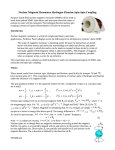
5.2.1 Method of Characteristics
The method of characteristics is a direct mathematical interpretation of the physical behaviour of the
cable. E. J. Routh proposed an early formulation of a dynamic cable model in 1905 (Johansson 1976).
A small segment 𝑑𝑠 of the cable is considered with its parametric trajectory 𝑥(𝑠), 𝑦(𝑠), 𝑧(𝑠) in terms of
Cartesian coordinates where 𝑠 is the trajectory curve length. 𝑑𝛿 is the unstretched length of 𝑑𝑠 so that
𝑑𝑠 = 𝑑𝛿(1 + 𝜖) where 𝜖 is the local strain. 𝑅 is the tension at the lower end of 𝑑𝑠, and the resolve
components along 𝑥, 𝑦, 𝑧 axes are
𝑅∙
𝑑𝑥
𝑑𝑦
𝑑𝑧
,𝑅 ∙
,𝑅 ∙
𝑑𝑠
𝑑𝑠
𝑑𝑠
The resolved tension components at the upper end are
𝑅∙
𝑑𝑥 𝑑
𝑑𝑥
+ (𝑅 ∙ ) 𝑑𝑠, 𝑒𝑡𝑐.
𝑑𝑠 𝑑𝑠
𝑑𝑠
The net tension force components thusly are
𝑑
𝑑𝑥
𝑑
𝑑𝑥
(𝑅 ∙ ) 𝑑𝑠 =
(𝑅 ∙ ) 𝑑𝛿, 𝑒𝑡𝑐.
𝑑𝑠
𝑑𝑠
𝑑𝛿
𝑑𝑠
Let 𝑚 be the mass per unit length of unstretched cable, and 𝑋, 𝑌, 𝑍 external force components per unit
of unstretched length. Also, let 𝑢, 𝑣, 𝑤 be the components of the segment velocity. The equations of
motion can then be written as
𝑚∙
𝜕𝑢
𝜕
𝑑𝑥
=
(𝑅 ∙ ) + 𝑋
𝜕𝑡 𝜕𝛿
𝑑𝑠
with corresponding equations for the 𝑦 and 𝑧 directions. 𝑡 represents time. For the submerged cable,
the hydrodynamic forces are included in 𝑋, 𝑌, 𝑍.
32
For two-dimensional problems, the equations may be expressed in terms of local tangential and
normal components in the form
𝜕𝑢
𝜕𝜙
𝜕𝑇
𝑚∙( −𝑣∙ )=𝑃+
𝜕𝑡
𝜕𝑡
𝜕𝛿
𝜕𝑣
𝜕𝜙
𝑇 𝜕𝑠
𝑚∙( +𝑢∙ )= 𝑄+ ∙
𝜕𝑡
𝜕𝑡
𝜌 𝜕𝛿
where 𝑃, 𝑄 are tangential and normal components of the external force, 𝑢, 𝑣 represents the tangential
and normal velocities and 𝜙 is the angle between the tangent and the horizontal plane or some other
fixed direction in the cable plane.
Through the integration of Routh’s equation along characteristic lines in 𝑥, 𝑦, 𝑧, 𝑡 space, for some
simple examples like straight strings, exact analytical solutions can be given. However, for problems
like lifting cable or mooring line, when cable experiences unsteady irregular external forces, a
stepwise computerized solution method is required but both over-detailed and time consuming. Most
of the time approximation is involved so that the accuracy is compromised.
5.2.2 Finite Element Methods
Finite Element Methods enable the cable to be conceptually modified (Johansson 1976) before
mathematical formulation. Comparison of different FEM cable models are given below.
 Mass-String: The cable is modelled as an inelastic string with mass lumped at several nodes.
 Mass-Spring: The cable is modelled as springs with mass lumped at several nodes.
 Bars: The cable is modelled as a series of straight bars with distributed mass, which are jointed
at both ends.
 Beams: The cable is modelled as a series of beams with distributed mass, which are jointed at
both ends and with additional internal curvature.
Mass-String
Mass-Spring
Beams
Bars
Figure 5.1 Four Types of FEM Cable Model
Table 5.1 Comparison of FEM Cable Models
Models
Mass-String
Elasticity
Mass
Moment of Inertia
Y
Mass-Spring
Bars
Beams
Y
Y
Y
Y
Y
Y
Y
Y
Plasticity
Slope Continuity
Structural Damping
Y
Y
Y
Tension Induced Torque
33
5.2.3 Linearization Method
In some stability and frequency response studies of cable vehicle systems, the motion equations are
linearized and assumed to only have small deviations from the state of equilibrium. The linear partial
differential equations will then be reduced to linear partial differential equations with curve length as
the space variable. Moreover, sometimes the perturbations are even assumed to be harmonic. Then
the time derivatives can be further eliminated from the equations, which become ordinary differential
equations solely about the cable length. In this thesis, the maximum length of lifting cable can reach
thousands of meters, which makes deformation along the cable significant and irregular. The
linearization method does not suit for this purpose.
5.3 Cable Model in 3D Mechanics
In this model, a combination of different types of FEM cable model is used in 3D Mechanics. The
cable is modelled as rigid bars with free rotational joint and 1-DOF translational joint on two ends
respectively. The rigid bars are represented by a inertia matrix which has both mass and moment of
inertia. The free rotational joint has no spring or damping but constrained all translational motions
between bars. The 1-DOF translational joint has spring and damping property which represent the
elasticity and structural damping of the cable respectively. The joint connecting the crane tip is free
rotational and the joint connecting to the load can be either free rotational or translational depending
on the structure of the connecting point. The elasticity, mass, moment of inertia and structural
damping of the cable are all realized in this modelling method.
If the number of discretized parts in FEM is 𝑛, the number of rigid bars, free rotational joint and 1-DOF
translational joint shall be 2𝑛, 𝑛, 𝑛 respectively, not including the joint on crane tip and load.
Figure 5.2 FEM Cable Model in 3D Mechanics
Using the same approach as in vessel motion input, the external forces such as current force and
buoyancy force can be applied as bond graph model on each rigid bar as a constant or the function of
motion and velocity. The port power should be defined in world coordinates, because of the coordinate
where current force is defined.
34
Figure 5.3 External Force Acting as Actuator
Outside the 3D Mechanics, each actuator is linked with a bond graph effort source where current force
and buoyancy force can be defined by simple Morison equation and Archimedes law or complex
expressions. The current speed is defined in a signal block by an array with length of 𝑛 or 2𝑛
depending on if two bars connected by translational joint shall have the same current speed.
Fix Tip & First Free Rotation Joint
Translational Joint
Element Bar
Actuator for current force and buoyancy
Position Sensor at the end of cable
Figure 5.4 Cable Model (n=3, L=10)
35
1
⃗ + 𝜌𝐶𝑑 𝐷 ∙ Δ𝐿(𝜇 − 𝜈) 𝜇 − 𝜈 )𝒊
𝐹 = 𝜌𝑔𝑉𝒌
2
𝜇𝐶 = [1,1]
Figure 5.5 External Force Input
36
6 LOAD MODEL
6.1 Lifting Operation
Offshore crane is designed to be multifunctional. The loading objects include subsea construction
materials, ROV, platform supplies, personnel carrier and all other different objects. Each loading
object has its unique physical property and installation requirement. The lifting operation can normally
be divided in five phases.
 Lift Off: The object is fixed to the cable and snatched from the deck. The major external forces
are friction from the deck, supporting force and lifting force.
 In Air: The object has been lifted and being moved to the designated position before being
lowered down into the water. The major external forces are air resistance, inertia force and lifting
force.
 Splashing: The object has been lowered close to the free water surface and experiencing
splashing impact until it is totally submerged and unaffected by the water surface. The major
external forces are splashing force, buoyancy force and lifting force.
 Deeply Submerged: The object is deeply submerged in the water yet still has a certain distance
from the seabed. The major external forces are buoyancy force, hydrodynamic force and lifting
force.
 Landing: The objected has been lowered close to the seabed and ready to land. The major
external forces are buoyancy, hydrodynamic force, lifting force and possibly landing impact force.
The object has its inertia matrix constantly through all phases, but different damping and restoring
functions respectively, e.g. the air resistance is mostly negligible while the object is in air but the
hydrodynamic resistance is significant in the water; the buoyancy force varies throughout the
splashing phase yet stays constant after the object is full submerged. In this thesis, a general method
of expressing the physical properties of the object in deeply submerged phase is given which can be
without loss of generality applied in other phases.
6.2 Load CFD
6.2.1 Motion Function of the Load
When an object is deeply submerged, it experiences a concentrated/scattered lifting force from the
cable, an evenly distributed gravity force downwards and buoyancy force upwards under the premise
of a constant submerged volume of which. It also experiences hydrodynamic forces including the
inertia force and the damping force by the definition in the Morison equation.
Similar to the ship motion equation, for a harmonically oscillating object, the motion function of an
submerged object in its own body fixed coordinate can be written as
𝑴𝑹𝑩 ∙ 𝜼̈ (𝑡) + 𝑴𝑨 (𝜔, 𝜁) ∙ 𝜼𝒓̈ (𝑡) + 𝑪𝑹𝑩 ∙ 𝜼̇ (𝑡) + 𝑪𝑨 (𝜔, 𝜁) ∙ 𝜼𝒓̇ (𝑡) + 𝑩(𝜔, 𝜁) ∙ 𝜼̇ 𝒓 (𝑡) 𝜼̇ 𝒓 (𝑡) = 𝝉𝒍 + 𝝉𝒈 + 𝝉𝒃
where
𝑴𝑹𝑩
𝜔
𝜁
𝑴𝑨 (𝜔, 𝜁)
𝑪𝑹𝑩
𝑪𝑨 (𝜔, 𝜁)
𝜼(𝑡)
𝜼𝒓 (𝑡)
𝑩(𝜔, 𝜁)
𝝉𝒍
𝝉𝒈
𝝉𝒃
= rigid body inertia matrix of the object
= oscillation frequency of the object
= oscillation amplitude of the object
= added mass matrix for a specific 𝜔 and 𝜁.
= coriolis force matrix of the object
= coriolis force matrix of the added mass for a specific 𝜔 and 𝜁
= object motion
= object relative motion to the fluid
= damping force matrix for a specific 𝜔 and 𝜁
= lifting force from the cable
= gravity force of the object
= buoyancy force of the object
The added mass matrix and the damping force matrix can be transformed into added mass coefficient
matrix 𝑴𝑨 (𝜔, 𝜁) and damping force coefficient 𝑩(𝜔, 𝜁) for a specific object with its unique shape. The
damping force here is by definition of Morison equation proportional to the square of velocity. The
37
calculation for a set of different frequencies and amplitudes can be done using CFD method (Halse, et
al. 2014)
6.2.2 Velocity & Acceleration Dependent Coefficient
The motion of the vessel model is assumed to be only periodic with constant added mass and
damping matrices for each frequency and amplitude. But the load could be lowered, lifted, dragged
and rotated without periodic feature. As the simulation is on a time-domain basis, the hydrodynamic
coefficients of the load should be transformed from frequency-amplitude dependent into velocityacceleration dependent 𝑴𝑨 (𝜼̇ , 𝜼̈ ) and 𝑩(𝜼̇ , 𝜼̈ ). Although the function is not strictly correct because the
fluid has memory effect, i.e. the historical motion of the fluid will affect the presence. But if a good
correlation can be shown by CFD calculation, the trajectory of the load can then be removed from the
variables.
To investigate the feasibility of velocity-acceleration dependent coefficients, a CFD experiment can be
conducted to compare the difference of coefficients under same velocity and acceleration condition
but with and without periodic movement.
Group A
Velocity-acceleration dependent
𝜼̇
𝑎11
…
𝑎𝑛1
𝜼̈
…
…
…
Group B
Amplitude-frequency dependent
𝑎1𝑛
…
𝑎𝑛𝑛
𝝎
𝑏11
…
𝑏𝑛1
𝜻
…
…
…
𝑏1𝑛
…
𝑏𝑛𝑛
if 𝜂̇ = 𝜔𝜁 𝑐𝑜𝑠(𝜔𝑡) & 𝜂̈ = −𝜔2 𝜁𝑠𝑖 𝑛(𝜔𝑡)
𝑎(𝜂̇ , 𝜂̈ ) = 𝑏(𝜔, 𝜁)?
Figure 6.1 CFD Experiment to Test & Verify Velocity-acceleration Dependent Coefficient
If valid, the velocity-acceleration dependent coefficients can then be fitted and input into 20-sim model
as functions of velocity and acceleration.
6.3 20-sim Modelling
In 20-sim 3D Mechanics, the loading object can be simply modelled as an object attached to the end
of the rope with an 6x1 actuator in body fixed coordinate representing extra added mass inertia force,
damping force and another 1x1 actuator in world coordinate representing buoyancy force.
Buoyancy Force
Added Mass and Damping Force
Figure 6.2 Load Model in 3D Mechanics
38
Figure 6.3 Buoyancy Force Actuator
The equation for the 1x1 buoyancy actuator is
𝑝. 𝑒 = 𝜌𝑔𝑉
Where 𝜌 is the water density, 𝑔 is the gravitational acceleration and 𝑉 is the submerged volume of the
load.
39
Figure 6.4 Added Mass and Damping Force Actuator
The setting inside 3D Mechanics only allows user to define diagonal inertia matrix for the object body,
while added mass is not always diagonal, so the added mass inertia force and coriolis force have to
be defined outside the 3D Mechanics. The equation for the 6x1 added mass and damping force
actuator is
𝒑. 𝒆 = −𝑴𝒂 (𝜼̇ , 𝜼̈ ) ∙ (𝒑. ̇ 𝒇 − 𝑼̇) − 𝑪𝑨 (𝜼̇ , 𝜼̈ ) ∙ (𝒑. 𝒇 − 𝑼) − 𝑩(𝜼̇ , 𝜼̈ ) ∙ (𝒑. 𝒇 − 𝑼) 𝒑. 𝒇 − 𝑼
with 𝑼 as the current velocity vector acting on the object.
The reason transformation jacobian 𝑱ℎ𝑏 is not used here is because added mass and damping
coefficient for an submerged object is constant with respect to the body fixed coordinate, while floating
object has a constant added mass and damping coefficient with respect to the steadily translating
coordinate.
40
Figure 6.5 Cable + Load Model
6.4 Model Assessment
To assess the accuracy and authenticity of the cable and load model, an evaluation between 3D
Mechanics model and standard DNV rules calculation is conducted. The 3D Mechanics model will
have a series number of discretized FEM parts 𝑛 and all parameters are set according to the
distribution of physical properties without manual tuning.
6.4.1 DNV Rules Calculation
According to DNV-RP-H103 5.2 (DNV 2010), the stretched length 𝐿𝑠 of a cable 𝐿 is
1
𝑊 + 𝑤𝐿
2 ] [𝑚]
𝐿𝑠 = 𝐿 [1 +
𝐸𝐴
where
𝐿𝑠
𝐿
𝑊
𝑤
𝑀
𝑚
𝑔
𝜌
𝐸
𝐴
𝑉
= stretched length of cable [m]
= original length of cable [m]
= 𝑀𝑔 − 𝜌𝑔𝑉 = fully submerged weight of lifted object [N]
= 𝑚𝑔 − 𝜌𝑔𝐴 = fully submerged weight per unit length of cable
= mass of lifted object [kg]
= mass per unit length of cable [kg/m]
= acceleration of gravity = 9.81 m/s2
= density of water [kg/m 3]
= modulus of elasticity of cable [N/m 2]
= nominal cross sectional area of cable [m 2]
= displaced volume of lifted object [m 3]
For an axially stiff cable with negligible bending stiffness the offset of a vertical cable with a heavy
weight at the end of the cable in an arbitrary current with unidirectional (x-direction) velocity profile is
𝑧1
1
𝐹𝐷0 + ( ) 𝜌 ∫−𝐿 𝐶𝐷𝑛 𝐷𝑐 [𝑈𝑐 (𝑧2 )]2 𝑑𝑧2
2
𝜁(𝑧) = ∫ [
] 𝑑𝑧1 [𝑚]
𝑊 + 𝑤(𝑧1 + 𝐿)
𝑧
0
where
1
𝐹𝐷0 = 𝜌𝐶𝐷𝑥 𝐴𝑥 [𝑈𝑐 (−𝐿)]2 [𝑁]
2
is the hydrodynamic damping force on the lifted object.
The parameters are defined as
41
𝜁(𝑧)
𝜁𝐿
𝐿
𝐶𝐷𝑛
𝐶𝐷𝑥
𝐷𝑐
𝐴𝑥
𝑈𝑐 (𝑧)
𝑧1, 𝑧2
= horizontal offset at vertical position z [m]
= horizontal offset at the end of cable z = -L [m]
= un-stretched length of cable [m]
= damping coefficient for normal flow past cable [-]
= damping coefficient for horizontal flow past lifted object [-]
= cable diameter [m]
= x-projected area of lifted object [m 2]
= current velocity at depth z [m/s]
= integration variables [m]
The formula can be transformed into
𝑧
𝛫+ +1
𝑞
𝑞
𝐿
𝜁(𝑧) = 𝐿 ( 𝛫 − 𝜆) 𝑙𝑛 [
]− 𝑧
𝑤
𝛫+1
𝑤
where
𝛫=
𝑊
𝑤𝐿
𝜆=
𝐹𝐷0
𝑤𝐿
𝑞=
1
𝜌𝐶 𝐷 𝑈 2
2 𝐷𝑛 𝑐 𝑐
6.4.2 FEM in 3D Mechanics
In 3D Mechanics, the length and mass of each rigid bar element for a cable length L is
𝛥𝐿 =
𝐿
;
2𝑛
𝛥𝑚 = 𝑚 ∙ 𝛥𝐿
The moment of inertia of each rigid bar element is
𝛥𝐼𝑥𝑥,𝑦𝑦 =
𝑚 ∙ 𝛥𝐿3
12
The axial moment of inertia Δ𝐼𝑧𝑧 is negligible.
The spring and damping coefficient of each rigid bar element are
Δ𝑘 = 𝐸𝐴/2Δ𝐿
Δ𝑐 = 2𝜁√(Δ𝑘 ∙ 𝑚)
6.4.3 Cable Parameters
The tested cable is Lankhorst Ropes’ 6x36 WS+IWRC standard wire rope with higher breaking
strength.
Table 6.1 6x36 WS+IWRC Parameters
Diameter [mm]
50
*including fluid friction
Weight [kg/m]
Elastic Modulus [GPa]
10.2
211
Structural Damping
Ratio per meter* [ζ]
0.1
Table 6.2 Parameters of Cable and Load
𝐶𝐷𝑛
𝐶𝐷𝑥
𝐴𝑥 [𝑚2 ]
1
1.2
3
* effective area ratio = 0.6
𝑀 [𝑘𝑔]
20000
𝑉 [𝑚3 ]
10
𝐴∗ [𝑚2 ]
0.001178
𝜌 [𝑘𝑔/𝑚3
1025
𝐸 [𝐺𝑃𝑎]
211
42
6.4.4 Results

Vertical Offset
Table 6.3 Vertical Offset with Lifted Load [m]
L=10 m
0.00387
0.00387
0.00387
0.00387
DNV
n=1
n=2
n=3
L=100 m
0.0403
0.0403
0.0403
0.0403
L=1000 m
0.562
0.562
0.562
0.562
 Horizontal Offset
The horizontal assessment was conducted with variables of FEM parts number, current speed and
linearity of the shape, i.e. without current force on load the cable will have higher nonlinearity of its
shape.
Horizontal Offset with Current Force on Load v=1m/s
0
DNV
n=1
n=2
n=3
-10
-20
-30
Depth m
-40
-50
-60
-70
-80
-90
-100
0
0.5
1
1.5
2
Offset m
2.5
3
3.5
Figure 6.6 Horizontal Offset with Current Force on Load V=1m/s
43
Horizontal Offset with Current Force on Load v=2m/s
0
DNV
n=1
n=2
n=3
-10
-20
-30
Depth m
-40
-50
-60
-70
-80
-90
-100
0
2
4
6
8
10
12
14
Offset m
Figure 6.7 Horizontal Offset with Current Force on Load V=2m/s
Horizontal Offset with Current Force on Load v=3m/s
0
DNV
n=1
n=2
n=3
-10
-20
-30
Depth m
-40
-50
-60
-70
-80
-90
-100
0
5
10
15
Offset m
20
25
30
Figure 6.8 Horizontal Offset with Current Force on Load V=3m/s
44
Horizontal Offset with Current Force on Load v=4m/s
0
DNV
n=1
n=2
n=3
-10
-20
-30
Depth m
-40
-50
-60
-70
-80
-90
-100
0
5
10
15
20
25
Offset m
30
35
40
45
50
Figure 6.9 Horizontal Offset with Current Force on Load V=4m/s
Horizontal Offset without Current Force on Load v=1m/s
0
DNV
n=1
n=2
n=3
-10
-20
-30
Depth m
-40
-50
-60
-70
-80
-90
-100
0
0.2
0.4
0.6
0.8
Offset m
1
1.2
1.4
Figure 6.10 Horizontal Offset without Current Force on Load V=1m/s
45
Horizontal Offset without Current Force on Load v=2m/s
0
DNV
n=1
n=2
n=3
-10
-20
-30
Depth m
-40
-50
-60
-70
-80
-90
-100
0
1
2
3
Offset m
4
5
6
Figure 6.11 Horizontal Offset without Current Force on Load V=2m/s
Horizontal Offset without Current Force on Load v=3m/s
0
DNV
n=1
n=2
n=3
-10
-20
-30
Depth m
-40
-50
-60
-70
-80
-90
-100
0
2
4
6
Offset m
8
10
12
Figure 6.12 Horizontal Offset without Current Force on Load V=3m/s
46
Horizontal Offset without Current Force on Load v=4m/s
0
DNV
n=1
n=2
n=3
-10
-20
-30
Depth m
-40
-50
-60
-70
-80
-90
-100
0
5
10
15
20
25
Offset m
Figure 6.13 Horizontal Offset without Current Force on Load V=4m/s
6.4.5 Discussion
 Vertical Offset
The FEM vertical offset had a perfect compliance with DNV rules no matter how much FEM parts were
set because both DNV rules calculation and FEM have analytical results of the problem. Thus for
cases where people only interest in vertical offset without current force, a single straight line with one
translational connector is sufficient enough.
 Horizontal Offset
The result shows that 1) under small horizontal offset condition (𝜁/𝐿 < 1: 5), the offset at the bottom
end of the cable has good compliance with DNV rules calculation result; 2) under large horizontal
offset condition (𝜁/𝐿 ≥ 1: 5), the bottom end of the cable has significant deviation from DNV rules
calculation result; 3) under small horizontal offset condition, nonlinearity shape of the cable trajectory
does not affect the accuracy of FEM model.
The reason for significant deviation under large horizontal offset condition is that by the definition of
DNV rules:
For an axially stiff cable with negligible bending stiffness the offset of a vertical cable with a heavy
weight at the end of the cable in an arbitrary current with unidirectional (x-direction) velocity profile is
𝑧1
1
𝐹𝐷0 + ( ) 𝜌 ∫−𝐿 𝐶𝐷𝑛 𝐷𝑐 [𝑈𝑐 (𝑧2 )]2 𝑑𝑧2
2
𝜁(𝑧) = ∫ [
] 𝑑𝑧1 [𝑚]
𝑊 + 𝑤(𝑧1 + 𝐿)
𝑧
0
the formula is only valid under small-angle approximation where the vertical depth of the cable equals
to the axial length of the cable,
sin 𝜃 ≈ 𝑡𝑎𝑛𝜃 ≈ 𝜃 𝑤ℎ𝑒𝑛 𝜃 𝑖𝑠 𝑠𝑚𝑎𝑙𝑙 𝑎𝑛𝑔𝑙𝑒
47
yet large horizontal offset cases (𝜁/𝐿 ≥ 1: 5) cannot be treated under small-angle approximation
anymore, where the resultant cable length under large horizontal offset is significantly longer than the
depth. The large horizontal offset condition also contradicts the premise of ‘a vertical cable with a
heavy weight at the end of the cable’ from the description of the formula.
However, the FEM model in 3D Mechanics is built according to a fixed cable length. Large horizontal
offset will cause the end of the cable to be lifted hence a smaller depth. From the small horizontal
offset cases the validity of FEM model has been proved. For large horizontal offset condition the FEM
model is still applicable for simulation purpose but requires extra evidence to support.
Since under small horizontal offset condition, the FEM model shows good compliance however the
parts number is, the choice of the part number only depends on the distribution of current force and
nonlinearity of the cable. Higher parts number will have better approximation of the shape, finer
distribution of the current force and more accurate dynamic simulation result. But it will also increase
the computation amount and time. The decision shall be made under different practical conditions.
48
7 SIMULATION EXAMPLE
All sub-models introduced in Chapter 3-6 can be assembled into one big model selectively. The
interactive physical entities are connected with power port whereas control loop are connected with
signal port. Some examples are demonstrated as follows. Because of the computation limits on
PC, hydraulic sub-model was replaced with direct PID control.
7.1 Vessel + Crane
7.1.1 Model
Figure 7.1 Simulation Example: Vessel + Crane
Figure 7.2 Animation: Vessel + Crane
49
7.1.2 Results
The default ship ‘s175’ from ShipX database is used. The video in the appendix showed the
anmimation of the target vessel (cyan) comparing with another vessel (grey) with SHIPX output
movement, under 10 s wave period, 60 deg heading and 1 m wave height. Figure 7.3 shows the
6DOF motion of vessel model in 20-sim during the start of the simulation (transient state).
Surge
0.2
0
-0.2
-0.4
0.6
Sway
0.4
0.2
0
-0.2
0.4
Heave
0.2
0
-0.2
-0.4
0.02
Roll
0.01
0
-0.01
-0.02
0.02
Pitch
0.01
0
-0.01
-0.02
0.03
Yaw
0.02
0.01
0
-0.01
0
50
100
150
200
250
300
time {s}
Figure 7.3 Vessel Motion: Vessel + Crane at Transient State
Figure 7.4 shows the roll motion of the vessel model during steady state (1000-1180 sec), which
means transient oscillation has died out.
Figure 7.5 shows the 6DOF motion of the vessel according to ShipX RAO. All motions are harmonic
signals meaning there is not distinction of transient or steady state.
50
Roll
0.005
0
-0.005
-0.01
1000
1020
1040
1060
1080
1100
1120
1140
1160
1180
time {s}
Figure 7.4 Vessel Motion: Vessel + Crane Roll at Steady State
0.2
Surge
0.1
0
-0.1
-0.2
0.2
Sway
0.1
0
-0.1
-0.2
0.4
Heave
0.2
0
-0.2
-0.4
0.008
Roll
0.004
0
-0.004
-0.008
0.02
Pitch
0.01
0
-0.01
-0.02
0.004
Yaw
0.002
0
-0.002
-0.004
0
50
100
150
200
250
300
time {s}
Figure 7.5 Vessel Motion: Vessel + Crane from SHIPX
51
7.1.3 Discussion
As the plot shows
1) There is deviation of 20-sim model from SHIPX RAO at the start of simulation, which is because the
model was at transient state, the vessel has both natural frequency oscillation and forced frequency;
2) The transient part of roll motion died out slower that the other motions because rolling has the
smallest damping of them all;
3) The deviation of surge, sway or yaw generated during the transient state will be kept during the
steady state because there is no restoring force for those three degrees of freedom.
4) After entering their steady state, the two sets of data (20-sim and SHIPX) have the identical
amplitude and frequency. For natural resonance cases mentioned in Chapter 3 where 20-sim model
has a deviated performance from ShipX RAO, the damping coefficient can be manually tuned
accordingly.
7.2 Vessel + Crane + Cable + Load
7.2.1 Model
Figure 7.6 Simulation Example: Vessel + Crane + Cable + Load
52
With addition of cable and load model, the interaction between the crane and vessel can be seen in
the simulation. Apart from vessel + crane animation, the video in the appendix also showed how
vessel is leaning to the crane side due to the effect of the heavy load (50 t & 100 t) . As for now, added
mass and damping of load model is set as constant. (𝐶𝑎 = 1; 𝐶𝑑 = 1.2)
Figure 7.7 Animation: Vessel + Crane + Cable + Load (100 t)
The dynamic behaviour of the cable and load is shown in another video because it is hard to identify
the effect in the entire model. Moreover, the cable model will significantly increase the complexity of
the model hence the computation amount. As stated in Chapter 6, for most cases, the cable can be
represented as an straight bar.
Figure 7.8 Animation: Dynamic Behaviour of Cable + Load
53
7.2.2 Results
Figure 7.9 shows the 6DOF motion of vessel model with cable and 50t of load in 20-sim during the
start of the simulation (transient state).
0.2
Surge
0
-0.2
-0.4
-0.6
0.6
Sway
0.4
0.2
0
-0.2
0.4
Heave
0.2
0
-0.2
-0.4
0
Roll
-0.02
-0.04
-0.06
-0.08
0.02
Pitch
0.01
0
-0.01
-0.02
Yaw
0.02
0.015
0.01
0.005
0
0
100
200
300
400
500
time {s}
Figure 7.9 Vessel Motion: Vessel + Crane + Cable + Load (50 t) at Transient State
Roll
-0.025
-0.03
-0.035
-0.04
-0.045
1000
1020
1040
1060
1080
1100
1120
1140
1160
1180
time {s}
Figure 7.10 Vessel Motion: Vessel + Crane + Cable + Load (50 t) Roll at Steady State
54
-0.06
Roll
-0.065
-0.07
-0.075
-0.08
1000
1020
1040
1060
1080
1100
1120
1140
1160
1180
time {s}
Figure 7.11 Vessel Motion: Vessel + Crane + Cable + Load (100 t) Roll at Steady State
Figure 7.10 and 7.11 show the roll motion of vessel model during transient state with the load weight
of 50t and 100t respectively.
7.2.3 Discussion
As the plot shows
1) After putting load and cable into the model, the roll motion of the vessel has higher irregularity at the
transient state and leans to the load side due to the pulling force.
2) The roll motions of the vessel with load of 50t or 100t have different steady angles (0.035/0.07 rad)
yet identical amplitude at steady state. This is because although the load is heavy enough to cause
dramatic leaning of the vessel, it is still not heavy enough to significantly change the natural frequency
of roll motion, and the damping coefficient of the vessel is constant regardless of the leaning angle.
Therefore the amplitude of the forced oscillation of the vessel will have no observable changes.
3) Motions without restoring force (surge, sway and yaw) continue to deviate in the steady state as a
result of the coupling effect between different degrees of freedom. Counter-measures including
potential dynamic positioning method is to be expected. The deviation is also due to the limited
integration accuracy during the simulation.
55
7.3 Vessel + Crane + Cable + Load + AHC
7.3.1 Model
Figure 7.12 Simulation Example: Vessel + Crane + Cable + Load + AHC
With the help of AHC system and possibly other control scheme, the crane can not only be manually
but also automatically controlled. The video in the appendix also showed how the load is being
controlled by AHC system.
7.3.2 Results
Figure 7.13 is the heave motion of the crane pedestal and the load without AHC system, from
transient state at the beginning to the steady state at the second half.
Figure 7.14 is the heave motion of the crane pedestal and the load with AHC system, from transient
state at the beginning to the steady state at the second half.
56
Figure 7.13 Load & Pedestal Heave: Vessel + Crane + Cable + Load (100 t)
57
Heave Motion with AHC
4
Load
Pedestal
2
0
-2
-4
-6
0
100
200
300
400
500
600
700
800
time {s}
Figure 7.14 Load & Pedestal Heave: Vessel + Crane + Cable + Load + AHC (100 t)
7.3.3 Discussion
As the plot shows
1) Without AHC system, the heave motions of the load and crane pedestal are identical, because the
crane does not have relative motion between them and the small deviation caused by rotational
motion can be ignored.
2) With the effect of AHC system, the load does not have good compensated motion at the beginning
of transient state, but the amplitude gradually decreases while entering to the steady state. This is
because the AHC system used in the model so far is based on crane kinematics, which has limitations
and response time. It has better performance towards regular and small motions rather than irregular
and drastic motions. Winch based AHC system may have different performance in this case, which
can be investigated in the future.
58
8 CONCLUSION & FUTURE WORK
8.1 Conclusion
This thesis demonstrated a generic modelling approach for marine operation. The aim is to propose a
standard application of modelling each sub-system in the marine operation however the design is. The
model consists of several modelling methods from other researchers yet with necessary modification
to make a compatible system. The general second order differential equation of vessel hydrodynamics
is from (Fossen and Fjellstad 2011). MATLAB files for ShipX data transformation is from (Fossen and
Perez 2014). Bond graph modelling technique is from (Pedersen 2008). Crane hydraulics and control
model is from (Chu 2013). Cable model inspired by (Johansson 1976). Load model inspired by (Halse,
et al. 2014). Combined the knowledge of previous researches, the modelling method proposed in this
thesis enables user to assemble all sub-models into a complete operation model. The complete model
can then be served for virtual dynamic analysis or training purpose. In the complete model, most of the
3D mechanics modelling are done inside the 3D Mechanics, a toolbox of 20-sim, but with connectors,
actuators and sensors, the 3D Mechanics model receives information and interacts with bond graph
and control scheme outside. The bond graph and control scheme expand the function of 3D
Mechanics model and give user the freedom to modify the design. The realistic physical entities
interacts as power flow and information interacts as signal flow, which gives a clear idea to separate
the different level of modelling. Besides crane, a winch, a propeller or a drilling tower can also be
modelled by following the same idea.
8.2 Future Work
As a part of the ongoing research, there are many things yet to be done. So far the modelling method
is still based on 20-sim, which has many restrictions, e.g. only diagonal matrix of inertia tensor is
allowed inside 3D Mechanics; only linear spring/damping is allowed inside 3D Mechanics; the function
of real-time interaction with Matlab has not been realised. In the future development, a better platform
or direct programming of physical engine may be required to expand the function of the model. Also, in
3D Mechanics, the model is eventually being solved as a big matrix yet only occupying single CPU
thread, which is time consuming and inefficient. Multithreads solution using GPU and parallel
computation should be applied in the future. The model also requires collision property and event
detector to control the different state of marine operation, e.g. crossing splash zone will have a
different model which requires splash model and detectors to detect the start and the end of the
phase.
The ideal model shall have the function of ‘Plug and Play’ which minimize the modelling procedure
and maximize the flexibility for different models. Thus, a standard interface between sub-models is
also required. Differernt parties shall have the same UI to develop their own sub-model, which in 3D
gaming industry often called as MOD (modification). Many sub-models can then be added into a
product library let users and customers to choose and test. Remote control and local PC experience is
also to be expected in the final package. There are still so much to be done.
59
REFERENCES
Norweigian Petroleum Directorate. 2010. «The petroleum sector – Norway’s largest industry.»
2014. Bond Graph. http://bondgraph.org/.
BP. 2013. “BP Statistical Review of World Energy June 2013.”
Chu, Yingguang. 2013. “20sim-based Simulation of Offshore Hyddraulic Crane Systems with Active
Heave Compensation and Anti-sway Control.”
Controllab Product BV. 2013. Hydraulic library, 20-sim Reference 4.3.
DNV. 2010. DNV-RP-H103 Modelling and analysis of marine operations, April 2010. DNV.
Euler, L. 1744. Methodus Inveniendi Lineas Curvas Maximi Minimive Proprietate Gaudentes sive
Solutio Problematis Isoperimetrici Latissimo Sensu Accepti. Laussanne and Geneva.
Fackrell, Shelagh. 2011. Study of the Added Mass of Cylinders and Spheres. University of Windsor.
Fagereng, Christian. 2011. «Mathematical Modeling for Marine Crane Operations.» Trondheim.
Fossen, Thor I., and Ola-Erik Fjellstad. 2011. Handbook of Marine Craft Hydrodynamics and Motion
Control. Trondheim: John Wiley & Sons, Ltd.
Fossen, Thor I., and Tristan Perez. 2014. MSS. Marine Systems Simulator (2010). 16 3.
http://www.marinecontrol.org.
Goldstein, H. 2001. Classical Mechanics (3rd ed.). Addison-Wesley.
Halse, Karl H., Vilmar Æsøy, Dimitry Ponkratov, Yingguang Chu, Jiafeng Xu, and Eilif Pedersen.
2014. Lifting Operations For Subsea Installations Using Small Construction Vessels and
Active Heave Compensation System - A Simulation Approach. OMAE.
Janssen, Sander. 2013. A Conversion from SolidWorks to 20-sim through COLLADA. Controllab
Product BV.
Johansson, Per I. 1976. A Finite Element Model for Dynamic Analysis of Mooring Cables.
Kirchhoff, G. R. 1877. Vorlesungen ueber Mathematische Physik, Mechanik. Leipzig.
Lloyd, A. R. J. M. 1989. Seakeeping: Ship Behaviour in rough weather. Ellis Horwood Limited.
Pedersen, Eilif. 2008. «Bond Graph Modeling of Marine Vehicle Dynamics.» Trondheim.
Sanfilippo, Filippo, Hans petter Hildre, Vilmar Æsøy, Hou Xiang Zhang, and Eilif Pederson. 2013.
“Flexible Modeling and Simulation Architecture for Haptic Control of Maritime Cranes and
Robotic Arms.”
Torby, Bruce J. 1984. Advanced Dynamics for Engineers. CBS College Publishing.
60
APPENDIX
Appendix A
User Manual
The manual explains the steps from ShipX calculation to *.mat file transfer and eventually 20-sim
simulation.
1.
Install MSS toolbox into your 32-bit Matlab. (see http://www.marinecontrol.org/download.html)
2.
Run SHIPX Veres, get .re1, .re2, .re7, .re8, .hyd data files (see
2008_06_19_MSS_vessel_models.pdf, page.18-20). If you do not have .re2 file, comment on
line 131 and line 136 in veres2vessel.m. the following calculation options and settings must be
chosen to comply with the MSS data structure.
i.
Ordinary strip theory (recommended but other methods can be used)
ii.
Added resistance – Gerritsma & Beukelman
iii.
Generate hydrodynamic coefficient files (*.re7 and *.re8)
iv.
Calculation options: choose z-coordinates from CO (Ob).
v.
Vessel velocities must always include the zero velocity: it is optional to add more
velocities that are needed for manoeuvring.
vi.
Wave periods: it is recommended to use values in the range 2.0s to 60.0s.
vii.
The wave heading must be chosen every 10 deg starting from 0 deg.
3.
Put SHIPX Veres data files, vereas2vessel.m, into the same folder and set it as the working
folder in Matlab.
4.
Type veres2vessel(‘input’) in Matlab, generate *.mat file (see
2008_06_19_MSS_vessel_models.pdf, page.20-21).
5.
Add 20SIM script toolbox 'library' and its subfolders into your Matlab toolbox path.
6.
Run simulation.m and follow the commands.
7.
Modify the 'parameters' block in 20SIM model to modify the rest parameters to run different
simulations.
8.
With 3D animation plot, you can directly compare the difference between results from SHIX
(grey) and 20SIM (cyan).
61
Appendix B

Matlab scripts
20-sim running
clear;
%% Connect to 20 SIM
xxsimConnect();
% Open the model Simple vessel.emx
fprintf('Please select a 20SIM model,press [Enter] to continue\n');
fprintf('\n');
pause;
[modelname,modelpath] = uigetfile({'*.emx','20SIM-Model(*.emx)'},'Select
20SIM Model');
% Check if the user pressed cancel on the dialog.
if isequal(modelname,0) || isequal(modelpath,0)
disp('Program cancelled');
return
else
disp(['User selected:', fullfile(modelpath, modelname)]);
end
xxsimOpenModel(fullfile(modelpath,modelname));
% process the model
xxsimProcessModel();
% Load *.mat data file
fprintf('Please select a SHIPX data, press [Enter] to continue\n');
fprintf('\n');
pause;
[dataname,datapath] = uigetfile({'*.mat','Matlab-data(*.mat)'},'Select
SHIPX data');
% Check if the user pressed cancel on the dialog.
if isequal(dataname,0) || isequal(datapath,0)
disp('Program cancelled');
return
else
disp(['User selected:', fullfile(datapath, dataname)]);
end
load(fullfile(datapath,dataname));
%% Select condition
% Define target vessel speed
knot = vessel.velocities/1.852*3.6;
fprintf('\nThe vessel speeds in knots are [');
fprintf('%g ',knot);
fprintf('\b].\n');
vel = str2num(input('Choose target vessel speed in knots:','s'));
for i=1:length(vessel.velocities)
if abs(vel-knot(i))<0.1
velno=i;
break
end
end
% Define target wave period
wp = 2*pi./vessel.freqs;
fprintf('\nThe wave periods are [');
fprintf('%g ',wp);
fprintf('\b].\n');
period = str2num(input('Choose wave period:','s'));
for j=1:length(vessel.freqs)
if abs(period-wp(j))<0.1
62
freqno=j;
break
end
end
% Define target wave heading
hd = vessel.headings*180/pi;
fprintf('\nThe wave headings are [');
fprintf('%g ',hd);
fprintf('\b].\n');
head = str2num(input('Choose wave heading:','s'));
for k=1:length(vessel.headings)
if abs(head-hd(k))<0.1
headno=k;
break
end
end
% ForceRAO
forceRAOamp = zeros(6,1);
forceRAOphase = zeros(6,1);
for i=1:6
forceRAOamp(i,1) = vessel.forceRAO.amp{i}(freqno,headno,velno);
forceRAOphase(i,1) = vessel.forceRAO.phase{i}(freqno,headno,velno);
end
% MotionRAO
motionRAOamp = zeros(6,1);
motionRAOphase = zeros(6,1);
for i=1:6
motionRAOamp(i,1) = vessel.motionRAO.amp{i}(freqno,headno,velno);
motionRAOphase(i,1) = vessel.motionRAO.phase{i}(freqno,headno,velno);
end
%% Curve for Ca and Cd of the object
% Za=rand(7,8); % CFD matrix for Ca, function of period and amplitude
% Zd=rand(7,8); % CFD matrix for Ca, function of period and amplitude
% p=3;
% q=3;
% aaCa=fitting(p,q,Za); % Curve fitting of Ca
% aaCd=fitting(p,q,Zd); % Curve fitting of Cd
Ca=1; % Added mass coefficient
Cd=1.2; % Damping coefficient
%% Set parameters
% Transfer nested variables
xxsimSetParameters({'g','Lpp','T',...
'rho','m','GML','GMT','Cb','Ca','Cd','MRB','DsubL',...
'Ma','C','forceRAOamp','forceRAOphase',...
'forceRAOw','motionRAOamp','motionRAOphase',...
'motionRAOw'},{vessel.main.g,vessel.main.Lpp,vessel.main.T,...
vessel.main.rho,vessel.main.m,vessel.main.GM_L,...
vessel.main.GM_T,vessel.main.C_B,Ca,Cd,vessel.MRB,...
vessel.B(:,:,freqno,velno),vessel.A(:,:,freqno,velno),...
vessel.C(:,:,freqno,velno),forceRAOamp,forceRAOphase,...
vessel.forceRAO.w(1,freqno),motionRAOamp,motionRAOphase,...
vessel.motionRAO.w(1,freqno)});
%% Run the model
xxsimRun();
63

DNV checking for cables
% Matlab script for calc. cable responses for crane operations
% Input variables
g = 9.81; % Acceleration of gravity (m/s^2)
rho = 1025; % density of water, (kg/m^3)
L = 100; % Length of cable (m)
D = 0.05; % Diameter of cable (m)
E = 2.1E11; % Youngs modulus (N/m^2)
A_c = pi*(D^2)/4; % Cross-section area (m^2)
A_eff = 0.6*A_c; % Effective area
%
% Mass of cable
m = 10.2; % Mass of cable (kg/m)
w = m*g-rho*g*A_eff; % weight of cable (in water) (N/m)
Cd_c = 1.0; % Drag coeff for cable
%
% Mass of load
M = 20000; % Mass of load (kg)
V=10;
W = M*g-rho*V*g; % Weight of load (N)
A_W =0; % Projected area of load (m^2)
Cd_W = 1.2; % Drag coeff for load
% Current velocity
U = 4; % Current velocity (m/s)
%
% ----------------------------------% Drag force on lifted object
Fd_load = 0.5*rho*Cd_W*A_W*U^2;
%
% Drag force per unit length of cable
q = 0.5* rho*Cd_c*D*U^2;
%
% Weight of Load/weight of cable
K = W / (w*L);
%
% Drag of Load/weight of cable
lambda = Fd_load / (w*L);
% -----------------------------------% Determine the shape of the cable
dz = 0.2; % Element length
z=0:dz:L;
% displ - function to calculate
% static displacement due to current
zeta = displ(-z,q,w,K,lambda,L);
Appendix C
20-sim models (digital)
Appendix D
Video footage of simulation (digital)
Appendix E
20-sim scripting library
64