1
NEST Topology User Manual
Hans Ekkehard Plesser
Håkon Enger
Department of Mathematical Sciences and Technology
Norwegian University of Life Sciences
1432 Ås, Norway
NEST 2.2 (r9977 or later)
About the Topology Module
This user manual gives a short introduction to the use of the Topology Module for the
NEST Neural Simulation Tool.
Rüdiger Kupper wrote a first topology library for NEST many years ago entirly in
SLI (actually, it pre-dates the NEST kernel). Kittel Austvoll and Hans Ekkehard Plesser
designed and wrote a completely new Topology library in 2007/8. That library has
been available with the NEST 1.9.x pre-releases since.
For NEST 2.0, Håkon Enger and Hans Ekkehard Plesser re-factored parts of the
Topology library code, improved and extended the PyNEST interface for the Topology
library, fixed bugs and added tests.
For NEST 2.2, Håkon Enger rewrote most of the Topology library code, thereby
improving performance considerably.
This User Manual describes the NEST 2.2 version of the NEST Topology Library.
Please see Chapter sec:changes for a summary of changes.
We plan further improvements to the Topology Module in the future, which may
include changes to the API to remove some of the remaining inconsistencies and provide a cleaner user interface.
c 2010 The NEST Initiative
Copyright Contents
1
Introduction
1.1 Limitations and Disclaimer . . . . . . . . . . . . . . . . . . . . . . . . . .
2
Layers
2.1 Grid-based Layers . . . . . . . . . . . . .
2.1.1 A very simple layer . . . . . . . .
2.1.2 Setting the extent . . . . . . . . .
2.1.3 Setting the center . . . . . . . . .
2.1.4 Constructing a layer: an example
2.2 Free layers . . . . . . . . . . . . . . . . .
2.3 3D layers . . . . . . . . . . . . . . . . . .
2.4 Periodic boundary conditions . . . . . .
2.4.1 Topology layer as NEST subnet .
2.5 Layers with composite elements . . . .
2.5.1 Designing layers . . . . . . . . .
.
.
.
.
.
.
.
.
.
.
.
.
.
.
.
.
.
.
.
.
.
.
.
.
.
.
.
.
.
.
.
.
.
.
.
.
.
.
.
.
.
.
.
.
.
.
.
.
.
.
.
.
.
.
.
.
.
.
.
.
.
.
.
.
.
.
.
.
.
.
.
.
.
.
.
.
.
.
.
.
.
.
.
.
.
.
.
.
.
.
.
.
.
.
.
.
.
.
.
.
.
.
.
.
.
.
.
.
.
.
.
.
.
.
.
.
.
.
.
.
.
.
.
.
.
.
.
.
.
.
.
.
.
.
.
.
.
.
.
.
.
.
.
.
.
.
.
.
.
.
.
.
.
.
.
.
.
.
.
.
.
.
.
.
.
.
.
.
.
.
.
.
.
.
.
.
.
.
.
.
.
.
.
.
.
.
.
.
.
.
.
.
.
.
.
.
.
.
.
.
.
.
.
.
.
.
.
.
.
4
4
4
6
6
6
7
9
9
11
11
12
Connections
3.1 Basic principles . . . . . . . . . . . . .
3.1.1 Terminology . . . . . . . . . . .
3.1.2 A minimal ConnectLayers call
3.2 Mapping source and target layers . . .
3.3 Masks . . . . . . . . . . . . . . . . . . .
3.3.1 Masks for 2D layers . . . . . .
3.3.2 Masks for 3D layers . . . . . .
3.3.3 Masks for grid-based layers . .
3.4 Kernels . . . . . . . . . . . . . . . . . .
3.5 Weights and delays . . . . . . . . . . .
3.6 Periodic boundary conditions . . . . .
3.7 Prescribed number of connections . .
3.8 Connecting composite layers . . . . .
3.9 Synapse models and properties . . . .
.
.
.
.
.
.
.
.
.
.
.
.
.
.
.
.
.
.
.
.
.
.
.
.
.
.
.
.
.
.
.
.
.
.
.
.
.
.
.
.
.
.
.
.
.
.
.
.
.
.
.
.
.
.
.
.
.
.
.
.
.
.
.
.
.
.
.
.
.
.
.
.
.
.
.
.
.
.
.
.
.
.
.
.
.
.
.
.
.
.
.
.
.
.
.
.
.
.
.
.
.
.
.
.
.
.
.
.
.
.
.
.
.
.
.
.
.
.
.
.
.
.
.
.
.
.
.
.
.
.
.
.
.
.
.
.
.
.
.
.
.
.
.
.
.
.
.
.
.
.
.
.
.
.
.
.
.
.
.
.
.
.
.
.
.
.
.
.
.
.
.
.
.
.
.
.
.
.
.
.
.
.
.
.
.
.
.
.
.
.
.
.
.
.
.
.
.
.
.
.
.
.
.
.
.
.
.
.
.
.
.
.
.
.
.
.
.
.
.
.
.
.
.
.
.
.
.
.
.
.
.
.
.
.
.
.
.
.
.
.
.
.
.
.
.
.
.
.
.
.
.
.
.
.
.
.
.
.
.
.
.
.
.
.
.
.
14
14
14
15
16
17
17
18
19
20
23
25
25
26
27
3
.
.
.
.
.
.
.
.
.
.
.
.
.
.
3
3
4
Inspecting Layers
29
4.1 Query functions . . . . . . . . . . . . . . . . . . . . . . . . . . . . . . . . . 29
4.2 Visualization functions . . . . . . . . . . . . . . . . . . . . . . . . . . . . . 30
5
Adding topology kernels and masks
32
5.1 Adding kernel functions . . . . . . . . . . . . . . . . . . . . . . . . . . . . 33
5.2 Adding masks . . . . . . . . . . . . . . . . . . . . . . . . . . . . . . . . . . 34
1
CONTENTS
2
6
Changes from Topology 2.0 to 2.2
37
7
Changes from Topology 1.9 to 2.0
38
Bibliography
39
List of Figures
40
List of Tables
41
Index
42
2
Chapter 1
Introduction
The Topology Module provides the NEST simulator1 (Gewaltig and Diesmann, 2007)
with a convenient interface for creating layers of neurons placed in space and connecting neurons in such layers with probabilities and properties depending on the relative
placement of neurons. This permits the creation of complex networks with spatial
structure.
This user manual provides an introdcution to the functionality provided by the
Topology Module. It is based exclusively on the PyNEST, the Python interface to NEST
(Eppler et al., 2008). NEST users using the SLI interface should be able to map instructions to corresponding SLI code. This manual is not meant as a comprehensive reference manual. Please consult the online documentation in PyNEST for details; where
appropriate, that documentation also points to relevant SLI documentation.
This manual describes the Topology Module included with NEST 2.2, code revision 9977 or later. This version differs from older ones in some important aspects as
detailed in Section 6. In our experience, though, most scripts using the Topology Module can be ported to the new version with minimal changes.
In the next chapter of this manual, we introduce Topology layers, which place neurons in space. In Chapter 3 we then describe how to connect layers with each other,
before discussing in Chapter 4 how you can inspect and visualize Topology networks.
Chapter 5 deals with the more advanced topic of extending the Topology module with
custom kernel functions and masks provided by C++ classes in an extension module.
You will find the Python scripts used in the examples in this manual in the NEST
source code directory under topology/doc/user_manual_scripts.
1.1
Limitations and Disclaimer
Undocumented features The Topology Module provides a number of undocumented
features, which you may discover by browsing the code. These features are
highly experimental and should not be used for simulations, as they have not been
validated.
1 NEST
is available under an open source license at www.nest-initiative.org.
3
Chapter 2
Layers
The Topology Module (just Topology for short in the remainder of this document)
organizes neuronal networks in layers. We will first illustrate how Topology places
elements in simple layers, where each element is a single model neuron. Layers with
composite elements are discussed in the following section.
We will illustrate the definition and use of layers using examples.
Topology distinguishes between two classes of layers:
grid-based layers in which each element is placed at a location in a regular grid;
free layers in which elements can be placed arbitrarily in the plane.
Grid-based layers allow for more efficient connection-generation under certain circumstances.
2.1
Grid-based Layers
2.1.1
A very simple layer
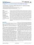
We create a first, grid-based simple layer with the following commands:
import n e s t . topology as tp
l = tp . CreateLayer ( { ’ rows ’
: 5,
’ columns ’ : 5 ,
’ elements ’ : ’ i a f _ n e u r o n ’ } )
The layer is shown in Fig. 2.1. Note the following properties:
• The layer has five rows and five columns.
• The ’elements’ entry of the dictionary passed to CreateLayer determines the elements of the layer. In this case, the layer contains iaf_neurons.
• The center of the layer is at the origin of the coordinate system, (0, 0).
• The extent or size of the layer is 1 × 1. This is the default size for layers. The
extent is marked by the thin square in Fig. 2.1.
4
2.1 Grid-based Layers
5
Figure 2.1: Simple grid-based layer centered about the origin. Blue circles mark layer
elements, the thin square the extent of the layer. Row and column indices are shown
in the right and top margins, respectively.
• The grid spacing of the layer is
x-extent
number of columns
y-extent
dy =
number of rows
dx =
(2.1)
In the layer shown, we have dx = dy = 0.2, but the grid spacing may differ in xand y-direction.
• Layer elements are spaced by the grid spacing and are arranged symmetrically
about the center.
• The outermost layer elements are placed dx/2 and dy/2 from the borders of the
extent.
• Element positions in the coordinate system are given by ( x, y) pairs. The coordinate system follows that standard mathematical convention that the x-axis runs
from left to right and the y-axis from bottom to top.
• Each element of a grid-based layer has a row- and column-index in addition to
its ( x, y)-coordinates. Indices are shown in the top and right margin of Fig. 2.1.
Note that row-indices follow matrix convention, i.e., run from top to bottom.
Following pythonic conventions, indices run from 0.
Note: The definition of the extent has changed from NEST 1.9 to NEST 2.0. In
NEST 1.9, the outermost elements of the layer were placed on the limits of the extent. When working with periodic boundary conditions (see Sec. 2.4), Topology then
silently padded the layer with half a grid spacing on all sides, to ensure that nodes at
opposite edges did not coincide.
5
2.1 Grid-based Layers
6
Figure 2.2: Same layer as in Fig. 2.1, but with different extent.
2.1.2
Setting the extent
Layers have a default extent of 1 × 1. You can specify a different extent of a layer, i.e.,
its size in x- and y-direction by adding and ’extent’ entry to the dictionary passed to
CreateLayer:
l = tp . CreateLayer ( { ’ rows ’
’ columns ’
’ extent ’
’ elements
:
:
:
’:
5,
5,
[2.0 , 0.5] ,
’ iaf_neuron ’ } )
The resulting layer is shown in Fig. 2.2. The extent is always a two-element tuple of
floats. In this example, we have grid spacings dx = 0.4 and dy = 0.1. Changing the
extent does not affect grid indices.
2.1.3
Setting the center
Layers are centered about the origin (0, 0) by default. This can be changed through the
’center’ entry in the dictionary specifying the layer. The following code creates layers
centered about (0, 0), (−1, 1), and (1.5, 0.5), respectively:
l 1 = tp . CreateLayer ( { ’ rows ’ :
l 2 = tp . CreateLayer ( { ’ rows ’ :
’ center
l 3 = tp . CreateLayer ( { ’ rows ’ :
’ center
5 , ’ columns ’ : 5 , ’ elements ’ : ’ i a f _ n e u r o n ’ } )
5 , ’ columns ’ : 5 , ’ elements ’ : ’ i a f _ n e u r o n ’ ,
’ : [ −1. ,1.]})
5 , ’ columns ’ : 5 , ’ elements ’ : ’ i a f _ n e u r o n ’ ,
’ : [1.5 ,0.5]})
The center is given as a two-element tuple of floats. Changing the center does not
affect grid indices: For each of the three layers in Fig. 2.3, grid indices run from 0 to
4 through columns and rows, respectively, even though elements in these three layers
have different positions in the gobal coordinate system.
2.1.4
Constructing a layer: an example
To see how to construct a layer, consider the following example:
• a layer with nr rows and nc columns;
• spacing between nodes is d in x- and y-directions;
6
2.2 Free layers
7
Figure 2.3: Three layers centered, respectively, about (0, 0) (blue), (−1, −1) (green),
and (1.5, 0.5) (red).
• the left edge of the extent shall be at x = 0;
• the extent shall be centered about y = 0.
From Eq. 2.1, we see that the extent of the layer must be (nc d, nr d). We now need to
find the coordinates (c x , cy ) of the center of the layer. To place the left edge of the
extent at x = 0, we must place the center of the layer at c x = nc d/2 along the x-axis,
i.e., half the extent width to the right of x = 0. Since the layer is to be centered about
y = 0, we have cy = 0. Thus, the center coordinates are (nc d/2, 0). The layer is created
with the following code and shown in Fig. 2.4:
nc , nr = 5 , 3
d = 0.1
l = tp . CreateLayer ( { ’ columns ’ : nc , ’ rows ’ : nr , ’ elements ’ : ’ i a f _ n e u r o n ’ ,
’ e x t e n t ’ : [ nc ∗d , nr ∗d ] , ’ c e n t e r ’ : [ nc ∗d / 2 . , 0 . ] } )
2.2
Free layers
Free layers do not restrict node positions to a grid, but allow free placement within the
extent. To this end, the user needs to specify the positions of all nodes explicitly. The
following code creates a layer of 50 iaf_neurons uniformly distributed in a layer with
extent 1 × 1, i.e., spanning the square [−0.5, 0.5] × [−0.5, 0.5]:
import numpy as np
pos = [ [ np . random . uniform ( − 0 . 5 , 0 . 5 ) , np . random . uniform ( − 0 . 5 , 0 . 5 ) ]
f o r j in xrange ( 5 0 ) ]
l = tp . CreateLayer ( { ’ p o s i t i o n s ’ : pos ,
’ elements ’ : ’ i a f _ n e u r o n ’ } )
Note the following points:
7
2.2 Free layers
8
Figure 2.4: Layer with nc = 5 rows and nr = 3 columns, spacing d = 0.1 and the left
edge of the extent at x = 0, centered about the y-axis. The cross marks the point on the
extent placed at the origin (0, 0), the circle the center of the layer.
Figure 2.5: A free layer with 50 elements uniformly distributed in an extent of size
1 × 1.
8
2.3 3D layers
9
Figure 2.6: A free 3D layer with 200 elements uniformly distributed in an extent of size
1 × 1 × 1.
• For free layers, element positions are specified by the ’positions’ entry in the dictionary passed to CreateLayer. ’positions’ is mutually exclusive with ’rows’/ ’columns’
entries in the dictionary.
• The ’positions’ entry must be a Python list (or tuple) of element coordinates, i.e.,
of two-element tuples of floats giving the (x, y)-coordinates of the elements. One
layer element is created per element in the ’positions’ entry.
• All layer element positions must be within the layer’s extent. Elements may be
place on the perimeter of the extent as long as no periodic boundary conditions
are used; see Sec. 2.4.
• Element positions in free layers are not shifted when specifying the ’center’ of
the layer. The user must make sure that the positions given lie within the extent
when centered about the given center.
2.3
3D layers
Although the term “layer” suggests a 2-dimensional structure, the layers in NEST
may in fact be 3-dimensional. The example from the previous section may be easily
extended with another component in the coordinates for the positions:
import numpy as np
pos = [ [ np . random . uniform ( − 0 . 5 , 0 . 5 ) , np . random . uniform ( − 0 . 5 , 0 . 5 ) ,
np . random . uniform ( − 0 . 5 , 0 . 5 ) ] f o r j in xrange ( 2 0 0 ) ]
l = tp . CreateLayer ( { ’ p o s i t i o n s ’ : pos ,
’ elements ’ : ’ i a f _ n e u r o n ’ } )
2.4
Periodic boundary conditions
Simulations usually model systems much smaller than the biological networks we
want to study. One problem this entails is that a significant proportion of neurons in a
9
2.4 Periodic boundary conditions
10
Figure 2.7: Top left: Layer with single row and five columns without periodic boundary conditions. Numbers above elements show element coordinates. Colors shifting
from blue to magenta mark increasing distance from the element at (−2, 0). Bottom
left: Same layer, but with periodic boundary conditions. Note that the element at
(2, 0) now is a nearest neighbor to the element at (−2, 0). Right: Layer with periodic
boundary condition arranged on a circle to illustrate neighborhood relationsships.
model network is close to the edges of the network with fewer neighbors than nodes
properly inside the network. In the 5 × 5-layer in Fig. 2.1, e.g., 16 out of 25 nodes form
the border of the layer.
One common approach to reducing the effect of boundaries on simulations is to
introduce periodic boundary conditions, so that the rightmost elements on a grid are
considered nearest neighbors to the leftmost elements, and the topmost to the bottommost. The flat layer becomes the surface of a torus. Fig. 2.7 illustrates this for a
one-dimensional layer, which turns from a line to a ring upon introduction of periodic
boundary conditions.
You specify periodic boundary conditions for a layer using the dictionary entry
edge_wrap:
l p = tp . CreateLayer ( { ’ rows ’ : 1 , ’ columns ’ : 5 , ’ e x t e n t ’ : [ 5 . , 1 . ] ,
’ elements ’ : ’ i a f _ n e u r o n ’ ,
’ edge_wrap ’ : True } )
Note that the longest possible distance between two elements in a layer without
periodic boundary conditions is
q
2 + y2
xext
ext
but only
q
2
xext
+ y2ext
2
for a layer with periodic boundary conditions; xext and yext are the components of the
extent size.
We will discuss the consequences of periodic boundary conditions more in Chapter 3.
10
2.5 Layers with composite elements
2.4.1
11
Topology layer as NEST subnet
From the perspective of NEST, a Topology layer is a special type of subnet. From the
user perspective, the following points may be of interest:
• Grid-based layers have the NEST model type topology_layer_grid, free layers the
model type topology_layer_free.
• The status dictionary of a layer has a ’topology’ entry describing the layer properties ( l is the layer created above):
p r i n t n e s t . GetStatus ( l ) [ 0 ] [ ’ topology ’ ]
{ ’ rows ’ : 5 , ’ c e n t e r ’ : [ 0 . 0 , 0 . 0 ] , ’ edge_wrap ’ : F a l s e , ’ depth ’ :
1 , ’ e x t e n t ’ : [ 1 . 0 , 1 . 0 ] , ’ columns ’ : 5 }
The ’topology’ entry is read-only.
• The NEST kernel sees the elements of the layer in the same way as the elements
of any subnet. You will notice this when printing a network with a Topology
layer:
n e s t . PrintNetwork ( depth =2)
+ − [0] r o o t dim=[1 2 5 ]
|
+ − [1] t o p o l o g y _ l a y e r _ g r i d dim = [ 2 5 ]
|
+ − [ 1 ] . . . [ 2 5 ] iaf_neuron
The 5 × 5 layer created above appears here as a topology_layer_grid subnet of
25 iaf_neurons. Only Topology connection and visualization functions heed the
spatial structure of the layer.
2.5
Layers with composite elements
So far, we have considered layers in which each element was a single model neuron.
Topology can also create layers with composite elements, i.e., layers in which each element is a collection of model neurons, or, in general NEST network nodes.
Construction of layers with composite elements proceeds exactly as for layers with
simple elements, except that the ’elements’ entry of the dictionary passed to CreateLayer
is a Python list or tuple. The following code creates a 1 × 2 layer (to keep the output
from PrintNetwork() compact) in which each element consists of one ’iaf_cond_alpha’
and one ’poisson_generator’ node
l = tp . CreateLayer ( { ’ rows ’ : 1 , ’ columns ’ : 2 ,
’ elements ’ : [ ’ i a f _ c o n d _ a l p h a ’ , ’ p o i s s o n _ g e n e r a t o r ’ ] } )
+ − [0] r o o t dim=[1 4 ]
|
+ − [1] t o p o l o g y _ l a y e r _ g r i d dim = [ 4 ]
11
2.5 Layers with composite elements
12
|
+ − [ 1 ] . . . [ 2 ] iaf_cond_alpha
+ − [ 3 ] . . . [ 4 ] poisson_generator
The network consist of one topology_layer_grid with four elements: two iaf_cond_alpha
and two poisson_generator nodes. The identical nodes are grouped, so that the subnet contains first one full layer of iaf_cond_alpha nodes followed by one full layer of
poisson_generator nodes.
You can create network elements with several nodes of each type by following a
model name with the number of nodes to be created:
l = tp . CreateLayer ( { ’ rows ’ : 1 , ’ columns ’ : 2 ,
’ elements ’ : [ ’ i a f _ c o n d _ a l p h a ’ , 1 0 , ’ p o i s s o n _ g e n e r a t o r ’ ,
’ noise_generator ’ , 2 ] } )
+ − [0] r o o t dim=[1 2 6 ]
|
+ − [1] t o p o l o g y _ l a y e r _ g r i d dim = [ 2 6 ]
|
+ − [ 1 ] . . . [ 2 0 ] iaf_cond_alpha
+ − [ 2 1 ] . . . [ 2 2 ] poisson_generator
+ − [23]...[26] noise_generator
In this case, each layer element consists of 10 iaf_cond_alpha neurons, one poisson_generator,
and two noise_generators.
Note the following points:
• Each element of a layer has identical components.
• All nodes within a composite element have identical positions, namely the position of the layer element.
• When inspecting a layer as a subnet, the different nodes will appear in groups of
identical nodes.
• For grid-based layers, the function GetElement returns a list of nodes at a given
grid position. See Chapter 4 for more on inspecting layers.
• In a previous version of the topology module it was possible to create layers with
nested, composite elements, but such nested networks gobble up a lot of memory
for subnet constructs and provide no practical advantages, so this is no longer
supported. See the next section for design recommendations for more complex
layers.
2.5.1
Designing layers
A paper on a neural network model might describe the network as follows1 :
1 See
Nordlie et al. (2009) for suggestions on how to describe network models.
12
2.5 Layers with composite elements
13
The network consists of 20x20 microcolumns placed on a regular grid spanning 0.5◦ × 0.5◦ of visual space. Neurons within each microcolumn are
organized into L2/3, L4, and L56 subpopulations. Each subpopulation
consists of three pyramidal cells and one interneuron. All pyramidal cells
are modeled as NEST iaf_neurons with default parameter values, while interneurons are iaf_neurons with threshold voltage Vth = −52mV.
How should you implement such a network using the Topology module? The recommended approach is to create different models for the neurons in each layer and then
define the microcolumn as one composite element:
f o r l y r in [ ’ L23 ’ , ’ L4 ’ , ’ L56 ’ ] :
n e s t . CopyModel ( ’ i a f _ n e u r o n ’ , l y r + ’ pyr ’ )
n e s t . CopyModel ( ’ i a f _ n e u r o n ’ , l y r + ’ i n ’ , { ’ V_th ’ : − 5 2 . } )
l = tp . CreateLayer ( { ’ rows ’ : 2 0 , ’ columns ’ : 2 0 , ’ e x t e n t ’ : [ 0 . 5 , 0 . 5 ] ,
’ elements ’ : [ ’ L23pyr ’ , 3 , ’ L23in ’ ,
’ L4pyr ’ , 3 , ’ L4in ’ ,
’ L56pyr ’ , 3 , ’ L56in ’ ] } )
We will discuss in Chapter 3.1 how to connect selectively to different neuron models.
13
Chapter 3
Connections
The most important feature of the Topology module is the ability to create connections
between layers with quite some flexibility. In this chapter, we will illustrate how to
specify and create connections. All connections are created using the ConnectLayers
function.
3.1
3.1.1
Basic principles
Terminology
We begin by introducing important terminology:
Connection In the context of connections between the elements of Topology layers,
we often call the set of all connections between pairs of network nodes created
by a single call to ConnectLayers a connection.
Connection dictionary A dictionary specifying the properties of a connection between
two layers in a call to CreateLayers.
Source The source of a single connection is the node sending signals (usually spikes).
In a projection, the source layer is the layer from which source node are chosen.
Target The target of a single connection is the node receiving signals (usually spikes).
In a projection, the target layer is the layer from which source node are chosen.
Connection type The connection type determines how nodes are selected when ConnectLayers
creates connections between layers. It is either ’convergent’ or ’divergent’.
Convergent connection When creating a convergent connection between layers, Topology visits each node in the target layer in turn and selects sources for it in the
source layer. Masks and kernels are applied to the source layer, and periodic
boundary conditions are applied in the source layer, provided that the source
layer has periodic boundary conditions.
Divergent connection When creating a divergent connection, Topology visits each node
in the source layer and selects target nodes from the target layer. Masks, kernels,
and boundary conditions are applied in the target layer.
14
3.1 Basic principles
15
Driver When connecting two layers, the driver layer is the one in which each node is
considered in turn.
Pool When connecting two layers, the pool layer is the one from which nodes are chosen for each node in the driver layer. I.e., we have
Pool
Connection type Driver
convergent
target layer source layer
divergent
source layer target layer
Displacement The displacement between a driver and a pool node is the shortest vector
connecting the driver to the pool node, taking boundary conditions into accout.
Distance The distance between a driver and a pool node is the length of their displacement.
Mask The mask defines which pool nodes are at all considered as potential targets for
each driver node. See Sec. 3.3 for details.
Kernel The kernel is a function returning a (possibly distance- or displacment-dependent)
probability for creating a connection between a driver and a pool node. The
default kernel is 1, i.e., connections are created with certainty. See Sec. 3.4 for
details.
Autapse An autapse is a synapse (connection) from a node onto itself. Autapses are
permitted by default, but can be disabled by adding ’allow_autapses’: False to the
connection dictionary.
Multapse Node A is connected to node B by a multapse if there are synapses (connections) from A to B. Multapses are permitted by default, but can be disabled by
adding ’allow_multapses’: False to the connection dictionary.
3.1.2
A minimal ConnectLayers call
Connections between Topology layers are created by calling ConnectLayers with the
following arguments1 :
1. The source layer.
2. The target layer (can be identical to source layer).
3. A connection dictionary that contains at least the following entries:
’connection_type’ Either ’convergent’ or ’divergent’.
’mask’ A mask specification as described in Sec. 3.3.
Here is a simple example, cf. 3.1:
1 You
can also use standard NEST connection functions to connect nodes in Topology layers.
15
3.2 Mapping source and target layers
16
Figure 3.1: Left: Minimal connection example from a layer onto itself using a rectangular mask shown as red line for the node at (0, 0) (marked light red). The targets of this
node are marked with red dots. The targets for the node at (4, 5) (marked light orange)
are marked with orange dots. This node has fewer targets since it is at the corner and
many potential targets are beyond the layer. Right: The effect of periodic boundary
conditions is seen here. Source and target layer and connection dictionary were identical, except that periodic boundary conditions were used. The node at (4, 5) now has
15 targets, too, but they are spread across the corners of the layer. If we wrapped the
layer to a torus, they would form a 5 × 3 rectangle centered on the node at (4, 5).
l = tp . CreateLayer ( { ’ rows ’ : 1 1 , ’ columns ’ : 1 1 , ’ e x t e n t ’ : [ 1 1 . , 1 1 . ] ,
’ elements ’ : ’ i a f _ n e u r o n ’ } )
conndict = { ’ connection_type ’ : ’ divergent ’ ,
’ mask ’ : { ’ r e c t a n g u l a r ’ : { ’ l o w e r _ l e f t ’ : [ − 2 . , − 1 . ] ,
’ upper_right ’ : [ 2 . , 1 . ] } } }
tp . ConnectLayers ( l , l , c o n n d i c t )
In this example, layer l is both source and target layer. Connection type is divergent,
i.e., for each node in the layer we choose targets according to the rectangular mask centered about each source node. Since no connection kernel is specified, we connect to all
nodes within the mask. Note the effect of normal and periodic boundary conditions
on the connections created for different nodes in the layer, as illustrated in Fig. 3.1.
3.2
Mapping source and target layers
The application of masks and other functions depending on the distance or even the
displacement between nodes in the source and target layers requires a mapping of
coordinate systems between source and target layers. Topology applies the following
coordinate mapping rules:
1. All layers have two-dimensional Euclidean coordinate systems.
2. No scaling or coordinate transformation can be applied between layers.
16
3.3 Masks
17
3. The displacement d( D, P) from node D in the driver layer to node P in the pool
layer is measured by first mapping the position of D in the driver layer to the
identical position in the pool layer and then computing the displacement from
that position to P. If the pool layer has periodic boundary conditions, they are
taken into account. It does not matter for displacement computations whether
the driver layer has periodic boundary conditions.
3.3
Masks
A mask describes which area of the pool layer shall be searched for nodes to connect
for any given node in the driver layer. We will first describe geometrical masks defined
for all layer types and then consider grid-based masks for grid-based layers.
Note that the mask size should not exceed the size of the layer when using periodic boundary conditions, since the mask would “wrap around” in that case and pool
nodes would be considered multiple times as targets.
If none of the mask types provided in the topology library meet your need, you
may add more mask types in a NEST extension module. This is covered in Chapter 5.
3.3.1
Masks for 2D layers
Topology currently provides three types of masks usable for 2-dimensional free and
grid-based layers. They are illustrated in Fig. 3.2. The masks are
Rectangular All nodes within a rectangular area are connected. The area is speficied
by its lower left and upper right corners, measured in the same unit as element
coordinates. Example:
conndict = { ’ connection_type ’ : ’ divergent ’ ,
’ mask ’ : { ’ r e c t a n g u l a r ’ : { ’ l o w e r _ l e f t ’ : [ − 2 . , − 1 . ] ,
’ upper_right ’ : [ 2 . , 1 . ] } } }
Circular All nodes within a circle are connected. The area is specified by its radius.
conndict = { ’ connection_type ’ : ’ divergent ’ ,
’ mask ’ : { ’ c i r c u l a r ’ : { ’ r a d i u s ’ : 2 . 0 } } }
Doughnut All nodes between an inner and outer circle are connected. Note that
nodes on the inner circle are not connected. The area is specified by the radii
of the inner and outer circles.
conndict = { ’ connection_type ’ : ’ divergent ’ ,
’ mask ’ : { ’ doughnut ’ : { ’ i n n e r _ r a d i u s ’ : 1 . 5 ,
’ outer_radius ’ : 3 . } } }
By default, the masks are centered about the position of the driver node, mapped into
the pool layer. You can change the location of the mask relative to the driver node by
specifying an ’anchor’ entry in the mask dictionary. The anchor is a 2D vector specifying the location of the mask center relative to the driver node, as in the following
examples (cf. Fig. 3.2, bottom row):
17
3.3 Masks
18
Figure 3.2: Masks for 2D layers. For all mask types, the driver node is marked by a
wide light-red circle, the selected pool nodes by red dots and the masks by red lines.
Top row from left to right: rectangular, circular and doughnut masks centered about
the driver node. Bottom row from left to right: the same masks as in the top row,
but centered about (−1.5, −1.5), (−2, 0) and (1.5, 1.5), respectively, using the ’anchor’
parameter.
conndict = { ’ connection_type ’ : ’ divergent ’ ,
’ mask ’ : { ’ r e c t a n g u l a r ’ : { ’ l o w e r _ l e f t ’ : [ − 2 . , − 1 . ] ,
’ upper_right ’ : [ 2 . , 1 . ] } ,
’ anchor ’ : [ − 1 . 5 , − 1 . 5 ] } }
conndict = { ’ connection_type ’ : ’ divergent ’ ,
’ mask ’ : { ’ c i r c u l a r ’ : { ’ r a d i u s ’ : 2 . 0 } ,
’ anchor ’ : [ − 2 . 0 , 0 . 0 ] } }
conndict = { ’ connection_type ’ : ’ divergent ’ ,
’ mask ’ : { ’ doughnut ’ : { ’ i n n e r _ r a d i u s ’ : 1 . 5 ,
’ outer_radius ’ : 3 . } ,
’ anchor ’ : [ 1 . 5 , 1 . 5 ] } }
3.3.2
Masks for 3D layers
Similarly, there are two mask types that can be used for 3D layers,
Box All nodes within a cuboid volume are connected. The area is speficied by its
18
3.3 Masks
19
Figure 3.3: Masks for 3D layers. For all mask types, the driver node is marked by a
wide light-red circle, the selected pool nodes by red dots and the masks by red lines.
From left to right: box and spherical masks centered about the driver node.
lower left and upper right corners, measured in the same unit as element coordinates. Example:
conndict = { ’ connection_type ’ : ’ divergent ’ ,
’ mask ’ : { ’ box ’ : { ’ l o w e r _ l e f t ’ : [ − 2 . , − 1 . , − 1 . ] ,
’ upper_right ’ : [ 2 . , 1 . , 1 . ] } } }
Spherical All nodes within a sphere are connected. The area is specified by its radius.
conndict = { ’ connection_type ’ : ’ divergent ’ ,
’ mask ’ : { ’ s p h e r i c a l ’ : { ’ r a d i u s ’ : 2 . 5 } } }
As in the 2D case, you can change the location of the mask relative to the driver node
by specifying a 3D vector in the ’anchor’ entry in the mask dictionary.
3.3.3
Masks for grid-based layers
Grid-based layers can be connected using rectangular grid masks. For these, you specify the size of the mask not by lower left and upper right corner coordinates, but give
their size in rows and columns, as in this example:
conndict = { ’ connection_type ’ : ’ divergent ’ ,
’ mask ’ : { ’ g r i d ’ : { ’ rows ’ : 3 , ’ columns ’ : 5 } } }
The resulting connections are shown in Fig. 3.4. By default the top-left corner of a
grid mask, i.e., the grid mask element with grid index [0, 0]2 , is aligned with the driver
node. You can change this alignment by specifying an anchor for the mask:
conndict = { ’ connection_type ’ : ’ divergent ’ ,
’ mask ’ : { ’ g r i d ’ : { ’ rows ’ : 3 , ’ columns ’ : 5 } ,
’ anchor ’ : { ’ row ’ : 1 , ’ column ’ : 2 } } }
2 See
Sec. 2.1.1 for the distinction between layer coordinates and grid indices
19
3.4 Kernels
20
Figure 3.4: Grid masks for connections between grid-based layers. Left: 5 × 3 mask
with default alignment at upper left corner. Center: Same mask, but anchored to center
node at grid index [1, 2]. Right: Same mask, but anchor to the upper left of the mask
at grid index [−1, 2].
You can even place the anchor outside the mask:
conndict = { ’ connection_type ’ : ’ divergent ’ ,
’ mask ’ : { ’ g r i d ’ : { ’ rows ’ : 3 , ’ columns ’ : 5 } ,
’ anchor ’ : { ’ row ’ : − 1, ’ column ’ : 2 } } }
The resulting connection patterns are shown in Fig. 3.4. Connections specified using
grid masks are generated more efficiently than connections specified using other mask
types.
Note the following:
• Grid-based masks are applied by considering grid indices. The position of nodes
in physical coordinates is ignored.
• In consequence, grid-based masks should only be used between layers with
identical grid spacings.
• The semantics of the ’anchor’ property for grid-based masks differ significantly
for general masks described in Sec. 3.3.1. For general masks, the anchor is the
center of the mask relative to the driver node. For grid-based nodes, the anchor
determines which mask element is aligned with the driver element.
3.4
Kernels
Many neuronal network models employ probabilistic connection rules. Topology supports probabilistic connections through kernels. A kernel is a function mapping the distance (or displacement) between a driver and a pool node to a connection probability.
Topology then generates a connections according to this probability.
Probabilistic connections can be generated in two different ways using Topology:
Free probabilistic connections are the default. In this case, ConnectLayers considers
each driver node D in turn. For each D, it evaluates the kernel for each pool node
P within the mask and creates a connection according to the resulting probability.
This means in particular that each possible driver-pool pair is inspected exactly once
and that there will be at most one connection between each driver-pool pair.
20
3.4 Kernels
21
Name
constant
Parameters
uniform
linear
min, max
a, c
Function
constant p ∈ [0, 1]
p ∈ [min, max) uniformly
p(d) = c + ad
exponential
a, c, tau
gaussian
p_center,
mean, c
gaussian2D
d
p(d) = c + ae− τ
sigma,
p(d) = c + pcenter e
p_center, sigma_x,
sigma_y, mean_x,
mean_y,rho c
p(d) = c + pcenter e
−
−
( d − µ )2
2σ2
(d x −µ x )(dy −µy )
( d x − µ x )2 ( d y − µ y )2
−
+2ρ
σx σy
σx2
σy2
2
2(1− ρ )
Table 3.1: Kernel functions currently available in the Topology module. d is the distance and (d x , dy ) the displacement.
Prescribed number of connections can be obtained by specifying the number of connections to create per driver node. See Sec. 3.7 for details.
Available kernel functions are shown in Table 3.1. More kernel function may be
created in a NEST extension module. This is covered in Chapter 5.
Several examples follow. They are illustrated in Fig. 3.5.
Constant The simplest kernel is a fixed connection probability:
conndict = { ’ connection_type ’ : ’ divergent ’ ,
’ mask ’ : { ’ c i r c u l a r ’ : { ’ r a d i u s ’ : 4 . } } ,
’ kernel ’ : 0 . 5 }
Gaussian This kernel is distance dependent. In the example, connection probability
is 1 for d = 0 and falls off with a “standard deviation” of σ = 1:
conndict = { ’ connection_type ’ : ’ divergent ’ ,
’ mask ’ : { ’ c i r c u l a r ’ : { ’ r a d i u s ’ : 4 . } } ,
’ k e r n e l ’ : { ’ g a u s s i a n ’ : { ’ p _ c e n t e r ’ : 1 . 0 , ’ sigma ’ : 1 . } } }
Excentric Gaussian In this example, both kernel and mask have been moved using
anchors:
conndict = { ’ connection_type ’ : ’ divergent ’ ,
’ mask ’ : { ’ c i r c u l a r ’ : { ’ r a d i u s ’ : 4 . } , ’ anchor ’ : [ 1 . 5 , 1 . 5 ] } ,
’ k e r n e l ’ : { ’ g a u s s i a n ’ : { ’ p _ c e n t e r ’ : 1 . 0 , ’ sigma ’ : 1 . ,
’ anchor ’ : [ 1 . 5 , 1 . 5 ] } } }
21
3.4 Kernels
22
Figure 3.5: Illustration of various kernel functions. Top left: constant kernel, p = 0.5.
Top center: Gaussian kernel, green dashed lines show σ, 2σ, 3σ. Top right: Same
Gaussian kernel anchored at (1.5, 1.5). Bottom left: Same Gaussian kernel, but all
p < 0.5 treated as p = 0. Bottom center: 2D-Gaussian.
Note that the anchor for the kernel is specified inside the dictionary containing
the parameters for the Gaussian.
Cut-off Gaussian In this example, all probabilties less than 0.5 are set to zero:
conndict = { ’ connection_type ’ : ’ divergent ’ ,
’ mask ’ : { ’ c i r c u l a r ’ : { ’ r a d i u s ’ : 4 . } } ,
’ k e r n e l ’ : { ’ g a u s s i a n ’ : { ’ p _ c e n t e r ’ : 1 . 0 , ’ sigma ’ : 1 . ,
’ cutoff ’ : 0 . 5 } } }
2D Gaussian We conclude with an example using a two-dimensional Gaussian, i.e., a
Gaussian with different widths in x- and y− directions. This kernel depends on
displacement, not only on distance:
conndict = { ’ connection_type ’ : ’ divergent ’ ,
’ mask ’ : { ’ c i r c u l a r ’ : { ’ r a d i u s ’ : 4 . } } ,
’ k e r n e l ’ : { ’ gaussian2D ’ : { ’ p _ c e n t e r ’ : 1 . 0 ,
’ sigma_x ’ : 1 . , ’ sigma_y ’ : 3 . } } }
Note that for pool layers with periodic boundary conditions, Topology always uses
the shortest possible displacement vector from driver to pool neuron as argument to
the kernel function.
22
3.5 Weights and delays
3.5
23
Weights and delays
The functions presented in Table 3.1 can also be used to specify distance-dependent or
randomized weights and delaysfor the connections created by ConnectLayers.
Figure 3.6 illustrates weights and delays generated using these functions with the
following code examples. All examples use a “layer” of 51 nodes placed on a line;
the line is centered about (25, 0), so that the leftmost node has coordinates (0, 0). The
distance between neighboring elements is 1. The mask is rectangular, spans the entire
layer and is centered about the driver node.
Linear example
l d i c t = { ’ rows ’ : 1 , ’ columns ’ : 5 1 ,
’ extent ’ : [ 5 1 . , 1 . ] , ’ center ’ : [ 2 5 . , 0 . ] ,
’ elements ’ : ’ i a f _ n e u r o n ’ }
c d i c t = { ’ connection_type ’ : ’ divergent ’ ,
’ mask ’ : { ’ r e c t a n g u l a r ’ : { ’ l o w e r _ l e f t ’ : [ − 2 5 . 5 , − 0 . 5 ] ,
’ upper_right ’ : [ 2 5 . 5 , 0 . 5 ] } } ,
’ weights ’ : { ’ l i n e a r ’ : { ’ c ’ : 1 . 0 , ’ a ’ : − 0.05 , ’ c u t o f f ’ : 0 . 0 } } ,
’ delays ’ : { ’ l i n e a r ’ : { ’ c ’ : 0 . 1 , ’ a ’ : 0 . 0 2 } } }
Results are shown in the top panel of Fig. 3.6. Connection weights and delays
are shown for the leftmost neuron as driver. Weights drop linearly from 1. From
the node at (20, 0) on, the cutoff sets weights to 0. There are no connections to
nodes beyond (25, 0) since as the mask extends only 25 units to the right of the
driver. Delays increase in a stepwise linear fashion, as NEST requires delays to
be multiples of the simulation resolution.
Linear example with periodic boundary conditions
c d i c t = { ’ connection_type ’ : ’ divergent ’ ,
’ mask ’ : { ’ r e c t a n g u l a r ’ : { ’ l o w e r _ l e f t ’ : [ − 2 5 . 5 , − 0 . 5 ] ,
’ upper_right ’ : [ 2 5 . 5 , 0 . 5 ] } } ,
’ weights ’ : { ’ l i n e a r ’ : { ’ c ’ : 1 . 0 , ’ a ’ : − 0.05 , ’ c u t o f f ’ : 0 . 0 } } ,
’ delays ’ : { ’ l i n e a r ’ : { ’ c ’ : 0 . 1 , ’ a ’ : 0 . 0 2 } } }
Results are shown in the middle panel of Fig. 3.6. This example is identical to the
previous, except that the (pool) layer has periodic boundary conditions. Therefore, the left half of the mask about the node at (0, 0) wraps back to the right half
of the layer and that node connects to all nodes in the layer.
Various functions
c d i c t = { ’ connection_type ’ : ’ divergent ’ ,
’ mask ’ : { ’ r e c t a n g u l a r ’ : { ’ l o w e r _ l e f t ’ : [ − 2 5 . 5 , − 0 . 5 ] ,
’ upper_right ’ : [ 2 5 . 5 , 0 . 5 ] } } ,
’ weights ’ : { ’ e x p o n e n t i a l ’ : { ’ a ’ : 1 . , ’ tau ’ : 5 . } } }
23
3.5 Weights and delays
24
Figure 3.6: Distance-dependent and randomized weights and delays. See text for details.
c d i c t = { ’ connection_type ’ : ’ divergent ’ ,
’ mask ’ : { ’ r e c t a n g u l a r ’ : { ’ l o w e r _ l e f t ’ : [ − 2 5 . 5 , − 0 . 5 ] ,
’ upper_right ’ : [ 2 5 . 5 , 0 . 5 ] } } ,
’ weights ’ : { ’ g a u s s i a n ’ : { ’ p _ c e n t e r ’ : 1 . , ’ sigma ’ : 5 . } } }
Results are shown in the bottom panel of Fig. 3.6. It shows linear, exponential
and Gaussian weight functions for the node at (25, 0).
Randomized weights and delays
c d i c t = { ’ connection_type ’ : ’ divergent ’ ,
’ mask ’ : { ’ r e c t a n g u l a r ’ : { ’ l o w e r _ l e f t ’ : [ − 2 5 . 5 , − 0 . 5 ] ,
’ upper_right ’ : [ 2 5 . 5 , 0 . 5 ] } } ,
’ weights ’ : { ’ uniform ’ : { ’ min ’ : 0 . 2 , ’max ’ : 0 . 8 } } }
By using the ’uniform’ function for weights or delays, one can obtain randomized
values for weights and delays, as shown by the red circles in the bottom panel
of Fig. 3.6. Weights and delays can currently only be randomized with uniform
distribution.
24
3.6 Periodic boundary conditions
3.6
25
Periodic boundary conditions
Connections between layers with periodic boundary conditions are based on the following principles:
• Periodic boundary conditions are always applied in the pool layer. It is irrelevant
whether the driver layer has periodic boundary conditions or not.
• By default, Topology does not accept masks that are wider than the pool layer
when using periodic boundary conditions. Otherwise, one pool node could appear as multiple targets to the same driver node as the masks wraps several
times around the layer. For layers with different extents in x- and y-directions
this means that the maximum layer size is determined by the smaller extension.
• Kernel, weight and delay functions always consider the shortest distance (displacement) between driver and pool node.
In most physical systems simulated using periodic boundary conditions, interactions
between entities are short-range. Periodic boundary conditions are well-defined in
such cases. In neuronal network models with long-range interactions, periodic boundary conditions may not make sense. In general, we recommend to use periodic boundary conditions only when connection masks are significantly smaller than the layers
they are applied to.
Important changes upon NEST 2.0:
• Prior to NEST 2.0, oversized masks were not prohibited by default and you may
have created networks with oversized masks by accident. You will now get a
NEST error message in this case. You can force Topology to accept oversized
masks by adding ’allow_oversized_mask’: True to the connection dictionary. Be
sure to inspect the results, e.g., using DumpLayerConnections.
• Distance- and displacement-dependent kernel, weight and delay functions did
not handle periodic boundary conditions correctly prior to NEST 2.0.
3.7
Prescribed number of connections
We have so far described how to connect layers by either connecting to all nodes inside the mask or by considering each pool node in turn and connecting it according
to a given probability function. In both cases, the number of connections generated
depends on mask and kernel.
Many neuron models in the literature, in contrast, prescribe a certain fan in (number
of incoming connections) or fan out (number of outgoing connections) for each node.
You can achieve this in Topology by prescribing the number of connections for each
driver node. For convergent connections, where the target layer is the driver layer,
you thus achieve a constant fan in, for divergent connections a constant fan out.
Connection generation now proceeds in a different way than before:
1. For each driver node, ConnectLayers randomly selects a node from the mask region in the pool layer, and creates a connection with the probability prescribed
by the kernel. This is repeated until the requested number of connections has
been created.
25
3.8 Connecting composite layers
26
2. Thus, if all nodes in the mask shall be connected with equal probability, you
should not specify any kernel.
3. If you specify a non-uniform kernel (e.g., Gaussian, linear, exponential), the connections will be distributed within the mask with the spatial profile given by the
kernel.
4. If you prohibit multapses (cf Sec. 3.1.1) and prescribe a number of connections
greater than the number of pool nodes in the mask, ConnectLayers may get stuck
in an infinte loop and NEST will hang. Keep in mind that the number of nodes
within the mask may vary considerably for free layers with randomly placed
nodes.
The following code generates a network of 1000 randomly placed nodes and connects them with a fixed fan out of 50 outgoing connections per node distributed with a
profile linearly decaying from unit probability to zero probability at distance 0.5. Multiple connections (multapses) between pairs of nodes are allowed, self-connections
(autapses) prohibited. The probability of finding a connection at a certain distance is
then given by the product of the probabilities for finding nodes at a certain distance
with the kernel value for this distance. For the kernel and parameter values below we
have
1
12
× 2πr × (1 − 2r ) = 24r (1 − 2r )
for 0 ≤ r < .
(3.1)
pconn (d) =
π
2
The resulting distribution of distances between connected nodes is shown in Fig. 3.7.
pos = [ [ np . random . uniform ( − 1 . , 1 . ) , np . random . uniform ( − 1 . , 1 . ) ]
f o r j in xrange ( 1 0 0 0 ) ]
l d i c t = { ’ p o s i t i o n s ’ : pos , ’ e x t e n t ’ : [ 2 . , 2 . ] ,
’ elements ’ : ’ i a f _ n e u r o n ’ , ’ edge_wrap ’ : True }
c d i c t = { ’ connection_type ’ : ’ divergent ’ ,
’ mask ’ : { ’ c i r c u l a r ’ : { ’ r a d i u s ’ : 1 . 0 } } ,
’ k e r n e l ’ : { ’ l i n e a r ’ : { ’ c ’ : 1 . , ’ a ’ : − 2. , ’ c u t o f f ’ : 0 . 0 } } ,
’ number_of_connections ’ : 5 0 ,
’ allow_multapses ’ : True , ’ a l l o w _ a u t a p s e s ’ : F a l s e }
Functions determining weight and delay as function of distance/displacement work
in just the same way as before when the number of connections is prescribed.
3.8
Connecting composite layers
Connections between layers with composite elements are based on the following principles:
• All nodes within a composite element have the same coordinates, the coordinates
of the element.
• All nodes within a composite element are treated equally. If, e.g., an element of
the pool layer contains three nodes and connection probability is 1, then connections with all three nodes will be created. For probabilistic connection schemes,
each of the three nodes will be considered individually.
26
3.9 Synapse models and properties
27
Figure 3.7: Distribution of distances between source and target for a network of 1000
randomly placed nodes, a fixed fan out of 50 connections and a connection probability
decaying linerarly from 1 to 0 at d = 0.5. The red line is the expected distribution from
Eq. 3.1.
• If only nodes of a given model within each element shall be considered as sources
or targets then this can be achieved by adding a ’sources’ or ’ targets ’ entry to the
connection dictionary, which speficies the model to connect.
This is exemplified by the following code, which connects pyramidal cells (pyr) to
interneurons (in) with a circular mask and uniform probablity and interneurons to
pyramidal cells with a rectangular mask unit probability.
n e s t . ResetKernel ( )
n e s t . CopyModel ( ’ i a f _ n e u r o n ’ , ’ pyr ’ )
n e s t . CopyModel ( ’ i a f _ n e u r o n ’ , ’ i n ’ )
l d i c t = { ’ rows ’ : 1 0 , ’ columns ’ : 1 0 , ’ elements ’ : [ ’ pyr ’ , ’ i n ’ ] }
cdi ct_p2 i = { ’ connection_type ’ : ’ divergent ’ ,
’ mask ’ : { ’ c i r c u l a r ’ : { ’ r a d i u s ’ : 0 . 5 } } ,
’ kernel ’ : 0.8 ,
’ s o u r c e s ’ : { ’ model ’ : ’ pyr ’ } ,
’ t a r g e t s ’ : { ’ model ’ : ’ i n ’ } }
cdi ct_i2 p = { ’ connection_type ’ : ’ divergent ’ ,
’ mask ’ : { ’ r e c t a n g u l a r ’ : { ’ l o w e r _ l e f t ’ : [ − 0 . 2 , − 0 . 2 ] , ’ u p p e r _ r i g h t ’ : [ 0
’ s o u r c e s ’ : { ’ model ’ : ’ i n ’ } ,
’ t a r g e t s ’ : { ’ model ’ : ’ pyr ’ } }
l = tp . CreateLayer ( l d i c t )
tp . ConnectLayers ( l , l , c d i c t _ p 2 i )
tp . ConnectLayers ( l , l , c d i c t _ i 2 p )
3.9
Synapse models and properties
By default, ConnectLayers creates connections using the default synapse model in NEST,
static_synapse. You can specify a different model by adding a ’synapse_model’ entry to
27
3.9 Synapse models and properties
28
the connection dictionary, as in this example:
n e s t . ResetKernel ( )
n e s t . CopyModel ( ’ i a f _ n e u r o n ’ , ’ pyr ’ )
n e s t . CopyModel ( ’ i a f _ n e u r o n ’ , ’ i n ’ )
n e s t . CopyModel ( ’ s t a t i c _ s y n a p s e ’ , ’ exc ’ , { ’ weight ’ :
2.0})
n e s t . CopyModel ( ’ s t a t i c _ s y n a p s e ’ , ’ inh ’ , { ’ weight ’ : − 8 . 0 } )
l d i c t = { ’ rows ’ : 1 0 , ’ columns ’ : 1 0 , ’ elements ’ : [ ’ pyr ’ , ’ i n ’ ] }
cdi ct_p2 i = { ’ connection_type ’ : ’ divergent ’ ,
’ mask ’ : { ’ c i r c u l a r ’ : { ’ r a d i u s ’ : 0 . 5 } } ,
’ kernel ’ : 0.8 ,
’ s o u r c e s ’ : { ’ model ’ : ’ pyr ’ } ,
’ t a r g e t s ’ : { ’ model ’ : ’ i n ’ } ,
’ synapse_model ’ : ’ exc ’ }
cdi ct_i2 p = { ’ connection_type ’ : ’ divergent ’ ,
’ mask ’ : { ’ r e c t a n g u l a r ’ : { ’ l o w e r _ l e f t ’ : [ − 0 . 2 , − 0 . 2 ] , ’ u p p e r _ r i g h t ’ : [ 0
’ s o u r c e s ’ : { ’ model ’ : ’ i n ’ } ,
’ t a r g e t s ’ : { ’ model ’ : ’ pyr ’ } ,
’ synapse_model ’ : ’ inh ’ }
l = tp . CreateLayer ( l d i c t )
tp . ConnectLayers ( l , l , c d i c t _ p 2 i )
tp . ConnectLayers ( l , l , c d i c t _ i 2 p )
You have to use synapse models if you want to set, e.g., the receptor type of connections or parameters for plastic synapse models. These can not be set in distancedependent ways at present.
28
Chapter 4
Inspecting Layers
We strongly recommend that you inspect the layers created by Topology to be sure
that node placement and connectivity indeed turned out as expected. In this chapter,
we describe some functions that NEST and Topology provide to query and visualize
networks, layers, and connectivity.
4.1
Query functions
The following table presents some query functions provided by NEST (nest. ) and
Topology (tp. ). For detailed information about these functions, please see the online
Python and SLI documentation.
nest.PrintNetwork()
nest.FindConnections()
nest.GetNodes()
nest.GetLeaves()
tp.GetPosition()
tp.GetLayer()
tp.GetElement()
tp.GetTargetNodes()
tp.GetTargetPositions()
tp.FindNearestElement()
tp.FindCenterElement()
Print structure of network or subnet from NEST
perspective.
Retrieve outgoing connections for a given source;
see also http://www.nest-initiative.org/index.
php/Connection_Management.
Applied to a layer, returns GIDs of the layer elements. For simple layers, these are the actual model
neurons, for composite layers the top-level subnets.
Applied to a layer, returns GIDs of all actual model
neurons, ignoring subnets.
Return the spatial locations of nodes.
Return the layer to which nodes belong.
Return the node(s) at the location(s) in the given
grid-based layer(s).
Obtain targets of a list of sources in a given target
layer.
Obtain positions of targets of a list of sources in a
given target layer.
Return the node(s) closest to the location(s) in the
given layer(s).
Return GID(s) of node closest to center of layer(s).
29
4.2 Visualization functions
tp.Displacement()
tp.Distance()
tp.DumpLayerNodes()
tp.DumpLayerConnections()
4.2
30
Obtain vector of lateral displacement between
nodes, taking periodic boundary conditions into account.
Obtain vector of lateral distances between nodes,
taking periodic boundary conditions into account.
Write layer element positions to file.
Write connectivity information to file. This function
may be very useful to check that Topology created
the correct connection structure.
Visualization functions
Topology provides three functions to visualize networks:
PlotLayer()
PlotTargets()
PlotKernel()
Plot nodes in a layer.
Plot all targets of a node in a given layer.
Add indication of mask and kernel to plot of layer.
It does not wrap masks and kernels with respect to
periodic boundary conditions. This function is usually called by PlotTargets.
The following code shows a practical example: A 21 × 21 network which connects to itself with divegent Gaussian connections. The resulting graphics is shown
in Fig. 4.1. All elements and the targets of the center neuron are shown, as well as
mask and kernel.
l = tp . CreateLayer ( { ’ rows ’ : 2 1 , ’ columns ’ : 2 1 ,
’ elements ’ : ’ i a f _ n e u r o n ’ } )
conndict = { ’ connection_type ’ : ’ divergent ’ ,
’ mask ’ : { ’ c i r c u l a r ’ : { ’ r a d i u s ’ : 0 . 4 } } ,
’ k e r n e l ’ : { ’ g a u s s i a n ’ : { ’ p _ c e n t e r ’ : 1 . 0 , ’ sigma ’ : 0 . 1 5 } } }
tp . ConnectLayers ( l , l , c o n n d i c t )
f i g = tp . P l o t L a y e r ( l , nodesize =80)
c t r = tp . FindCenterElement ( l )
tp . P l o t T a r g e t s ( c t r , l , f i g = f i g ,
mask= c o n n d i c t [ ’ mask ’ ] , k e r n e l = c o n n d i c t [ ’ k e r n e l ’ ] ,
s r c _ s i z e =250 , t g t _ c o l o r = ’ red ’ , t g t _ s i z e =20 ,
k e r n e l _ c o l o r = ’ green ’ )
30
4.2 Visualization functions
31
Figure 4.1: 21 × 21 grid with divergent Gaussian projections onto itself. Blue circles
mark layer elements, red circles connection targets of the center neuron (marked by
large light-red circle). The large red circle is the mask, the dashed green lines mark σ,
2σ and 3σ of the Gaussian kernel.
31
Chapter 5
Adding topology kernels and masks
This chapter will show examples of how to extend the topology module by adding
custom kernel functions and masks. Some knowledge of the C++ programming language is needed for this. The functions will be added as a part of an extension module
which is dynamically loaded into NEST. For more information on writing an extension
module, see the section titled “Writing an Extension Module” in the NEST Developer
Manual. The basic steps required to get started are:
1. From the NEST source directory, copy directory examples/MyModule to somewhere outside the NEST source, build or install directories.
2. Change to the new location of MyModule and prepare by issuing ./bootstrap.sh
3. Leave MyModule and create a build directory for it, e.g., mmb next to it
cd . .
mkdir mmb
cd mmb
4. Configure. The configure process uses the script nest−config to find out where
NEST is installed, where the source code resides, and which compiler options
were used for compiling NEST. If nest−config is not in your path, you need to
provided it explicitly like this
. . / MyModule/ c o n f i g u r e −−with−n e s t =$ { NEST_INSTALL_DIR}/ bin/nest −c o n f i g
5. MyModule will then be installed to ${NEST_INSTALL_DIR}. This ensures that
NEST will be able to find initializing SLI files for the module. You should not
use the −−prefix to select a different installation destination. If you do, you must
make sure to use addpath in SLI before loading the module to ensure that NEST
will find the SLI initialization file for your module.
6. Compile.
make
make i n s t a l l
The previous command installed MyModule to the NEST installation directory,
including help files generated from the source code.
32
5.1 Adding kernel functions
5.1
33
Adding kernel functions
As an example, we will add a kernel function called ’affine2d’ , which will be linear
(actually affine) in the displacement of the nodes, on the form
p(d) = ad x + bdy + c.
The kernel functions are provided by C++ classes subclassed from nest :: Parameter. To
enable subclassing, add the following lines at the top of the file mymodule.h:
# include " topologymodule . h "
# include " parameter . h "
Then, add the class definition, e.g. near the bottom of the file before the brace closing
the namespace mynest:
c l a s s Affine2DParameter : public n e s t : : Parameter
{
public :
Affine2DParameter ( c o n s t DictionaryDatum& d ) :
Parameter ( d ) ,
a_ ( 1 . 0 ) ,
b_ ( 1 . 0 ) ,
c_ ( 0 . 0 )
{
updateValue <double >(d , " a " , a_ ) ;
updateValue <double >(d , " b " , b_ ) ;
updateValue <double >(d , " c " , c_ ) ;
}
double raw_value ( c o n s t n e s t : : P o s i t i o n <2>& disp ,
librandom : : RngPtr&) c o n s t
{
r e t u r n a_ ∗ disp [ 0 ] + b_∗ disp [ 1 ] + c_ ;
}
n e s t : : Parameter ∗ c l o n e ( ) c o n s t
{ r e t u r n new Affine2DParameter ( ∗ t h i s ) ; }
private :
double a_ , b_ , c_ ;
};
The class contains a constructor, which reads the value of the parameters a, b and c
from the dictionary provided by the user. The function updateValue will do nothing if
the given key is not in the dictionary, and the default values a = b = 1, c = 0 will be
used.
The overridden method raw_value() will return the actual value of the kernel function for the displacement given as the first argument, which is of type nest :: Position<2>.
33
5.2 Adding masks
34
The template argument 2 refers to a 2-dimensional position. You can also implement
a method taking a nest :: Position<3> as the first argument if you want to support 3dimensional layers. The second argument, a random number generator, is not used in
this example.
The class also needs to have a clone() method, which will return a dynamically
allocated copy of the object. We use the (default) copy constructor to implement this.
To make the custom function available to the Topology module, you need to register the class you have provided. To do this, add the line
n e s t : : TopologyModule : : r e g i s t e r _ p a r a m e t e r <Affine2DParameter >( " a f f i n e 2 d " ) ;
to the function MyModule::init() in the file mymodule.cpp. Now compile and install the
module by issuing
make
make i n s t a l l
To use the function, the module must be loaded into NEST using nest. Install () . Then,
the function is available to be used in connections, e.g.
n e s t . I n s t a l l ( ’ mymodule ’ )
l = tp . CreateLayer ( { ’ rows ’ : 1 1 , ’ columns ’ : 1 1 , ’ e x t e n t ’ : [ 1 . , 1 . ] ,
’ elements ’ : ’ i a f _ n e u r o n ’ } )
tp . ConnectLayers ( l , l , { ’ c o n n e c t i o n _ t y p e ’ : ’ convergent ’ ,
’ mask ’ : { ’ c i r c u l a r ’ : { ’ r a d i u s ’ : 0 . 5 } } ,
’ kernel ’ : { ’ affine2d ’ : { ’ a ’ : 1.0 , ’b ’ : 2.0 , ’ c ’ : 0 . 5 } } } )
5.2
Adding masks
The process of adding a mask is similar to that of adding a kernel function. A subclass
of nest :: Mask<D> must be defined, where D is the dimension (2 or 3). In this case we
will define a 2-dimensional elliptic mask by creating a class called EllipticMask. First,
we must include another header file:
# include " mask . h "
Compared to the Parameter class discussed in the previous section, the Mask class has
a few more methods that must be overridden:
c l a s s E l l i p t i c M a s k : public n e s t : : Mask<2>
{
public :
E l l i p t i c M a s k ( c o n s t DictionaryDatum& d ) :
rx_ ( 1 . 0 ) , ry_ ( 1 . 0 )
{
updateValue <double >(d , " r_x " , rx_ ) ;
updateValue <double >(d , " r_y " , ry_ ) ;
}
using Mask < 2 > : : i n s i d e ;
34
5.2 Adding masks
35
/ / returns true i f point is inside the e l l i p s e
bool i n s i d e ( c o n s t n e s t : : P o s i t i o n <2> &p ) c o n s t
{ r e t u r n p [ 0 ] ∗ p [ 0 ] / rx_/rx_ + p [ 1 ] ∗ p [ 1 ] / ry_/ry_ <= 1 . 0 ; }
/ / r e t u r n s t r u e i f t h e w h o l e box i s i n s i d e t h e e l l i p s e
bool i n s i d e ( c o n s t n e s t : : Box<2> &b ) c o n s t
{
n e s t : : P o s i t i o n <2> p = b . l o w e r _ l e f t ;
/ / T e s t i f a l l c o r n e r s a r e i n s i d e mask
i f ( not i n s i d e ( p ) ) r e t u r n f a l s e ;
/ / (0
p [ 0 ] = b . upper_right [ 0 ] ;
i f ( not i n s i d e ( p ) ) r e t u r n f a l s e ;
/ / (0
p [ 1 ] = b . upper_right [ 1 ] ;
i f ( not i n s i d e ( p ) ) r e t u r n f a l s e ;
/ / (1
p[0] = b . lower_left [ 0 ] ;
i f ( not i n s i d e ( p ) ) r e t u r n f a l s e ;
/ / (1
,0)
,1)
,1)
,0)
return true ;
}
/ / r e t u r n s b o u n d i n g box o f e l l i p s e
n e s t : : Box<2> get_bbox ( ) c o n s t
{
n e s t : : P o s i t i o n <2> l l (− rx_ , − ry_ ) ;
n e s t : : P o s i t i o n <2> ur ( rx_ , ry_ ) ;
r e t u r n n e s t : : Box <2 >( l l , ur ) ;
}
n e s t : : Mask<2> ∗ c l o n e ( ) c o n s t
{ r e t u r n new E l l i p t i c M a s k ( ∗ t h i s ) ; }
protected :
double_t rx_ , ry_ ;
};
The overridden methods include a test if a point is inside the mask, and for efficiency
reasons also a test if a box is fully inside the mask. We implement the latter by testing if
all the corners are inside, since our elliptic mask is convex. We must also define a function which returns a bounding box for the mask, i.e. a box completely surrounding the
mask.
Similar to kernel functions, the mask class must be registered with the topology
module, and this is done by adding a line to the function MyModule::init() in the file
mymodule.cpp:
n e s t : : TopologyModule : : r e g i s t e r _ m a s k < E l l i p t i c M a s k >( " e l l i p t i c " ) ;
35
5.2 Adding masks
36
After compiling and installing the module, the mask is available to be used in connections, e.g.
n e s t . I n s t a l l ( ’ mymodule ’ )
l = tp . CreateLayer ( { ’ rows ’ : 1 1 , ’ columns ’ : 1 1 , ’ e x t e n t ’ : [ 1 . , 1 . ] ,
’ elements ’ : ’ i a f _ n e u r o n ’ } )
tp . ConnectLayers ( l , l , { ’ c o n n e c t i o n _ t y p e ’ : ’ convergent ’ ,
’ mask ’ : { ’ e l l i p t i c ’ : { ’ r_x ’ : 0 . 5 , ’ r_y ’ : 0 . 2 5 } } } )
36
Chapter 6
Changes from Topology 2.0 to 2.2
This is a short summary of the most important changes in the Topology Module from
NEST version 2.0 to 2.2.
• Nested layers are no longer supported.
• Subnets are no longer used inside composite layers. A call to GetElement for a
composite layer will now return a list of GIDs for the nodes at the position rather
than a single subnet GID.
• Positions in layers may now be 3-dimensional.
• The functions GetPosition, Displacement and Distance now only works for nodes
local to the current MPI process, if used in a MPI-parallel simulation.
• It is now possible to add kernel functions and masks to the Topology module
through an extension module. Please see Chapter 5 for examples.
37
Chapter 7
Changes from Topology 1.9 to 2.0
This is a short summary of the most important changes in the NEST Topology Module
from the 1.9-xxxx to the 2.0 version.
• ConnectLayer is now called ConnectLayers
• Several other functions changed names, and there are many new functions. Please
see Ch. 4 for an overview.
• All nest.topology functions now require lists of GIDs as input, not "naked" GIDs
• There are a number of new functions in nest.topology, I tried to write good doc
strings for them
• For grid based layers (ie those with /rows and /columns), we have changed the
definition of "extent": Previously, nodes were placed on the edges of the extent,
so if you had an extend of 2 (in x-direction) and 3 nodes, these had x-coordinates
-1, 0, 1. The grid constant was extent/(num_nodes - 1).
Now, we define the grid constant as extent/num_nodes, center the nodes about
0 and thus add a space of half a grid constant between the outermost nodes and
the boundary of the extent. If you want three nodes at -1,0,1 you thus have to set
the extent to 3, i.e., stretching from -1.5 to 1.5.
The main reason for this change was that topology always added this padding
silently when you used periodic boundary conditions (otherwise, neurons are
the left and right edge would have been in identical locations, not what one
wants).
• The semantics of the anchor entry for kernel functions has changed: the anchor
now specifies the center of the probability distribution relative to the driver node.
This is consistent with the semantics for free masks, see Sec. 3.3 and 3.4.
• Functions computing connection probabilities, weights and delays as functions
of distance between source and target nodes now handle periodic boudary conditions correctly.
• Masks with a diameter larger than the diameter of the layer they are applied to
are now prohibited by default. This avoids multiple connections when masks
overwrap.
38
Bibliography
Jochen Martin Eppler, Moritz Helias, Eilif Muller, Markus Diesmann, and Marc-Oliver
Gewaltig. PyNEST: A convenient interface to the NEST simulator. Front Neuroinformatics, 2:12, 2008. doi: 10.3389/neuro.11.012.2008.
M.-O. Gewaltig and M. Diesmann. Nest (neural simulation tool). Scholarpedia, 2(4):
1430, 2007.
Eilen Nordlie, Marc-Oliver Gewaltig, and Hans Ekkehard Plesser. Towards reproducible descriptions of neuronal network models. PLoS Comput Biol, 5(8):e1000456,
Aug 2009. doi: 10.1371/journal.pcbi.1000456.
39
List of Figures
2.1
2.2
2.3
2.4
2.5
2.6
2.7
Simple grid-based layer . . . . . . . .
Layer with non-standard extent . . . .
Layers with different centers . . . . . .
Layer construction example . . . . . .
Layer with freely spaced elements. . .
3D layer with freely spaced elements.
Periodic boundary conditions. . . . . .
.
.
.
.
.
.
.
.
.
.
.
.
.
.
.
.
.
.
.
.
.
.
.
.
.
.
.
.
.
.
.
.
.
.
.
.
.
.
.
.
.
.
.
.
.
.
.
.
.
.
.
.
.
.
.
.
.
.
.
.
.
.
.
. 5
. 6
. 7
. 8
. 8
. 9
. 10
3.1
3.2
3.3
3.4
3.5
3.6
3.7
Minimal connection example . . . . . . . . . . . . . . . .
Masks for 2D layers . . . . . . . . . . . . . . . . . . . . . .
Masks for 3D layers . . . . . . . . . . . . . . . . . . . . . .
Grid masks . . . . . . . . . . . . . . . . . . . . . . . . . . .
Kernel functions . . . . . . . . . . . . . . . . . . . . . . . .
Distance-dependent and randomized weights and delays
Distribution of connection distances . . . . . . . . . . . .
.
.
.
.
.
.
.
.
.
.
.
.
.
.
.
.
.
.
.
.
.
.
.
.
.
.
.
.
.
.
.
.
.
.
.
.
.
.
.
.
.
.
.
.
.
.
.
.
.
.
.
.
.
.
.
.
.
.
.
.
.
.
.
4.1
Example of layer visualization. . . . . . . . . . . . . . . . . . . . . . . . . 31
40
.
.
.
.
.
.
.
.
.
.
.
.
.
.
.
.
.
.
.
.
.
.
.
.
.
.
.
.
.
.
.
.
.
.
.
.
.
.
.
.
.
.
.
.
.
.
.
.
.
.
.
.
.
.
.
.
.
.
.
.
.
.
.
.
.
.
.
.
.
.
16
18
19
20
22
24
27
List of Tables
3.1
Kernel functions . . . . . . . . . . . . . . . . . . . . . . . . . . . . . . . . . 21
41
Index
2D Gaussian kernel, 21
3D layers, 9, 18
free probabilistic connections, 20
adding kernels and masks, 33
anchor, 17, 19
autapse, 15
Gaussian kernel, 20
grid mask, 19
grid spacing, 5
grid-based layer, 4
box, 18
hang, 26
center, 4, 6
circular, 17
columns, 4
composite element, 11, 27
connection, 14
connection dictionary, 14
connection type, 14
ConnectLayers, 14, 15
constant kernel, 20
convergent connection, 14
coordinate mapping rules, 16
coordinate system, 5, 16
coordinates, 27
cut-off kernel, 21
index, 5
infinite loop, 26
delays, stepwise, 23
displacement, 15
distance, 15
distance-dependent weight, 23
distance-dependent delay, 23
divergent connection, 14
doughnut, 17
driver, 15
egde_wrap, 10
element, 4
excentric kernel, 21
extent, 4
fan in, 26
fan out, 26
free layer, 7
kernel, 15, 20, 34
layer, 4
mapping, 16
mask, 15, 35
model, 27
multapse, 15, 26
oversized mask, 26
periodic boundary cond., 10, 16, 23, 24
pool, 15
position, 5, 9
prescribed number of connections, 26
probabilistic connection rules, 20
randomized delay, 23
randomized weight, 23
rectangular, 17
row, 4
source, 14
source layer, 14
spherical, 19
subnet, 11
synapse model, 28
target, 14
target layer, 14
topology_layer_free, 11
topology_layer_grid, 11
42