Download efnmr

Nuclear Magnetic Resonance Hydrogen-Fluorine Spin-Spin Coupling
Purpose: Earth-field nuclear magnetic resonance (NMR) will be used to
learn about pulsed NMR. Spin-lattice and spin-spin relaxation times of
protons in water will be measured. The hydrogen-fluorine nuclear spin
coupling constant in liquid trifluoroethanol will also be measured.
Introduction
Nuclear magnetic resonance is a field of complicated theory and many
applications. Professor Paul Callaghan wrote the following in his introductory remarks1 about NMR:
The scope of magnetic resonance is daunting, partly because the interactions of atomic
nuclei with their atomic and molecular surroundings are subtle and diverse, and partly
because the ways in which the nuclei can be made to respond to those terms by virtue of
externally applied electromagnetic fields is almost boundless. The designer of magnetic
resonance pulse sequences has at his or her disposal the depth of complexity possible
when a composer writes a score for an orchestra.
This experiment uses a simple low-field instrument to study two fundamental aspects of NMR: spin
relaxation and spin-spin coupling.
Theory
Many atomic nuclei have intrinsic spin. Hydrogen and fluorine, specifically the isotopes 1H and 19F,
have nuclear spins of ½. This experiment observes transitions of nuclear spins of hydrogen and fluorine
under the influence of a magnetic field.
The spin quantum number is I, the quantum number for the z component of spin is m, and spin states
are α and β.
ℏ
1
^I 2 α = I ( I +1)ℏ2 α = 3 ℏ 2 α
m= + : ^I z α = m ℏ α =
α ;
2
2
4
(1)
ℏ
1
3 2
2
2
^
^
m= − : I z β = m ℏ β = − β ;
I β = I (I +1) ℏ β = ℏ β
2
2
4
E
Nuclear-spin energy levels in an external magnetic field B0 are simply m = −m γ ℏ B0 , where γ is
the magnetogyric ratio. For 1H, γ=2.675×108 T−1 s−1 .[Engel and Reid,2 Table 28.1] For 19F,
3
8 −1 −1
γ=2.517×10 T s [Halse, Magritek ] Considering that m=±½, energies are simply ± ½ ℏ γ B 0 ,
up-spin α is lower in energy than down-spin β. The energy difference is Δ E = E−1/2− E1 /2 = γ ℏ B0 .
As usual in spectroscopy, Δ E =h ν =ℏ ω ; this ω is the "Larmor" frequency.
ω = γ B0
(2)
-1
Note: ω is radians per second; ν=ω /(2 π) is in Hertz = Hz = s .
Nuclear spins act as though they are magnetic moments precessing around the magnetic
field B0. Up-spins, α, are partially aligned with B0 and precess in the positive direction, as
per the right-hand rule. Down-spins, β, are partially anti-parallel to B0 and precess in the
opposite direction. The z direction is defined by the direction of B0.
EFNMR.odt
1
When many spins add together, as do those of the hydrogen nuclei in a sample of water, the net
magnetization is along B0. A collection of N spins at temperature T will, at equilibrium, have net
magnetization M:
M = N γ ℏ ⟨ m⟩
(3)
where <m>, the average z-component spin quantum number, is given by statistical thermodynamics.
m=+1 /2
∑
⟨ m⟩ =
m=−1/ 2
m=+1 /2
∑
−m γ ℏ B0 /(k B T )
me
−m γ ℏ B 0 /(k B T )
(4)
e
m=−1/ 2
Magnetization is so weak (because both γ and B0 are small) that M simplifies to the following:
2 2
N γ ℏ B0
(5)
M=
2 kB T
For this experiment, it is worth noting that M is proportional to γ 2 , so proton spectra should be more
intense than fluorine spectra, for the same number of nuclei. In fact, the intensity ratio is γ 3 rather
than just γ 2 because detection relies on voltage induced in the B1 coil, and that voltage (called Vout
below) is proportional to γ .
When taking a spectrum, the sample's spin magnetic moment M (which is the net sum of all the
precessing nuclear magnetic moments) is first enhanced with a "polarizing" field Bp created by the
outer magnet. The Bp pulse also tips M from the z axis onto the y axis. Magnetization M is initially
directed along the Earth's magnetic field, which defines the z direction. Polarization field is along the x
axis, which is the longitudinal axis of the instrument. Recall that, by the right-hand rule, z crossed into
x generates torque in the y direction. The polarizing pulse is long enough and strong enough that it both
increases the amplitude of M and reorients M to y.
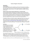
After the polarizing pulse, M begins to relax in two ways: Mz returns slowly to its equilibrium value
along the z axis, and (Mx,My) begin to "dephase". Dephasing refers to the individual nuclear magnetic
moments, which were
temporarily aligned along M,
spreading out. The time constant
for that spread is T2. The time
constant for re-growth of Mz, the
relaxation known as spin-lattice
relaxation, is T1. Often, T1 is
greater than T2. Component Mz
is not detected by our
instrument, so T1 is not directly
Figure 1: The polarizing field Bp enhances M and tips it 90o.
observed. The component of M
Dephasing then spreads M with time constant T2*.
in the (x,y) plane is detected by
the B1 coil. The sketches in
Figure 1 are like those shown by Engel and Reid in their Section 28.13.2
EFNMR.odt
2
The effective, or observed, spin-spin relaxation time is T2*. It is related to the true spin-lattice time T2
and field inhomogeneity, ΔB0. Inhomogeneity shortens T2*. Great inhomogeneity may make T2* so
short that no signal at all is observed. Shimming fields along the x, y and z directions are added to
reduce ΔB0, and so increase T2*. With our instrument located in room 301 of the Chemistry building,
effective spin-spin relaxation times may be as long as a few seconds.
1
1
=
+ γ Δ B0
(6)
*
T
T2
2
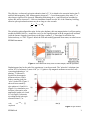
The polarizing pulse aligned the spins. As the spins dephase, their net magnetization is still precessing
around the Earth's field (i.e., around the z axis), so the signal detected in the B1 magnet both oscillates
(with the Larmor frequency) and decays (with time constant T2*). That signal is called the free
induction decay, or "FID". Figure 2 shows the FID and resulting spectrum from water, recorded on our
EFNMR instrument.
Figure 2. Free-induction decay from a water sample, and the spectrum.
Dephasing need not be the end of the experiment; it can be reversed. The "spin echo" technique (see
section 28.13 of reference 2) uses a 180o (or "π") pulse to flip magnetic moments across the x axis,
converting dephasing to "rephasing." Coherence is
regained as the magnetic
moments refocus, which
leads to another peak (the
"echo") in the FID. Figure 3
shows echoes caused by
echo pulses at 0.2 and 0.6 s.
(Figure 3 is a simulation, not
real data.) Successive echo
amplitudes (peaks at 0.4, and
0.8 s in Figure 3) decrease
according the the spin-spin
relaxation time T2, as
−t /T 2
echo
. (7)
∝e
amplitude
EFNMR.odt
Figure 3. spin echoes
3
Successive echoes weaken because only the "inhomogeneous" dephasing due to field inhomogeneity
and chemical shift is recovered by spin reversal; true "homogeneous" spin-spin relaxation is not.
The spin-lattice (or "longitudinal") relaxation time, T1, can be measured by varying the time between
the polarizing pulse Bp and a subsequent 90o pulse. In the context of NMR, "lattice" simply means the
surroundings with which spins can exchange energy. Suppose the magnetization along the z direction is
Mz at time t, and that its equilibrium value is ME, where the subscript "E" refers to the Earth's magnetic
field. As spins exchanges energy with their surroundings, Mz changes like so:
d Mz
M E− M z
=
(8)
dt
T1
A solution to equation 8 is
−t /T 1
M z (t) = M z (0) e
(
−t /T 1
+ME 1 − e
)
(9)
Because the polarizing pulse has a magnetic field much greater than the Earth's field, M z (0)≫M E ,
the second term on the right-hand size can be neglected. That is,
(10)
−t /T 1
M z (t) = M z (0) e
.
The magnetization at time t is proportional to the FID amplitude at time t after the polarizing pulse.
One can simply apply a 90o pulse at time t, measure the initial amplitude. After repeating the
experiment with several values of t, ln(Mz(t)) can be graphed versus t; the slope equals -1/T1.
Figure 4. Pulse sequence for T1 in the Earth's field.
In addition to measuring spin-spin and spin-lattice relaxation times, this experiment will record
resonances of fluorine and hydrogen nuclei in 2,2,2-trifluoroethanol. The spin-spin coupling constant,
J, of H and F nuclei will also be measured. (The constant may be called 3J or J3 because the H and F
nuclei are separated by three bonds.) Chemical shifts will not be observed. The OH proton and the CH2
protons will appear at the same resonant frequency because chemical shifts of a few parts per million
are too small resolve in our low-field NMR. For example, a shift of 5 ppm from a resonant frequency
of 2000 Hz is a shift of only 0.01 Hz. That is much smaller than our instrument's peak widths of
approximately 1 Hz.
Proton and fluorine peaks will split into multiplets because of spin-spin coupling. The hydroxyl proton
is not involved in this splitting because the OH proton exchanges rapidly between alcohol molecules
and any traces of water present in the sample. The multiplets, then arise from three F nuclei interacting
with two H nuclei; a 1:2:1 triplet and a 1:3:3:1 quartet. The following simple analysis relies on H and F
resonances being well separated, with the H-F interaction then added on. In frequency units (Hz, units
of ν or ω/2π) the frequency shift due to H-F interaction is Δν.
EFNMR.odt
4
Δ ν = mH m F J
The additivity condition (that interactions are "first order") is easy to check after spectra
have been recorded.
|ω H − ω F|
J≪
2π
(11)
(12)
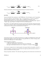
Figure 5 shows first the energy
levels (but in frequency units,
ν=E/h) of an F nucleus and a pair
of H nuclei, then the energy levels
of FH2 nuclei, but without
interaction (i.e., with J=0). The
third set of energy levels adds
energy shifts due to interaction, as
given in equation 6. Because the
two H nuclei are treated as a pair,
their mH quantum numbers are -1,
0 and +1, corresponding to H
nuclear spin configurations αα,
αβ, βα, and ββ, respectively.
A similar analysis predicts that the
CH2 proton resonance splits into a
1:3:3:1 quartet, with frequency
spacing J. The remaining proton,
the hydroxyl proton, will still be
at the unshifted proton resonance,
so the protons will appear as a
Figure 5. FH2 energy levels and transitions.
quartet (1:3:3:1) centered on a
singlet of relative intensity 4 (i.e., a 1:3:4:3:1 intensity pattern). Engel and Reid discuss AX2 and AX3
cases in section 28.8.2
Within the same first-order approximation used to predict splitting patterns, peak intensities are simply
3
proportional to the number of nuclei and to γ . If a spectrum is not too noisy, the integrated area
under a peak is a good measure of its intensity. Trifluoroethanol contains the same number of fluorine
and hydrogen nuclei but fluorine has a smaller γ , so the integral of fluorine peaks should be smaller
than the integral of hydrogen peaks.
EFNMR.odt
5
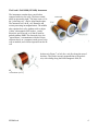
The Earth's Field NMR (EFNMR) Instrument
The instrument contains three coaxial tubes
wrapped with wire, the coils. The three coaxial
tubes are pictured at right.3 The large outer coil is
the "polarizing coil," used to align sample spins.
The innermost coil, the B1 coil, measures and
excites precessing net magnetization. The middle
tube contains four coils: gradient coils to adjust
("shim") the magnetic field in the x, y and z
directions, and a second x coil that is used for
pulsed-gradient NMR. The electronics box, the
"spectrometer," communicates with the Prospa
software that is on a computer, sends power to the
coils as needed, and collects response from the B1
coil.
Figure 6. Magritek EFNMR coils (ref. 3)
As shown in Figure 7, at left, the x axis lies along the axes of
the tubes. The y and z axes are perpendicular to the probe's
axis, with z being along the Earth's magnetic field, BE.
Figure 7. EFNMR probe and axis
conventions. (ref. 3)
EFNMR.odt
6
Reagents
500 mL of deionized water
500 mL of 2,2,2-trifluorethanol
in the lab on tap
in the lab
Procedure
setup and shim the EFNMR instrument
The EFNMR may already be in place; check to be sure. The
EFNMR on its plastic cart should be between benches, with
the coil axis perpendicular to magnetic N-S. (There is a
conventional compass for locating North.) The arrow on the
end of the instrument should point along the magnetic field
(there is a three-axis compass for the purpose), likely a little
off vertical.
Turn on the spectrometer. Start the Prospa software on the
computer. Connect the usb cable from the spectrometer to the
computer. Prepare to use a flash drive to save data and
images from the experiment.
Figure 8. placement of the EFNMR
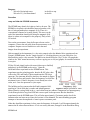
With no sample in the instrument (i.e., the cavity empty) select the MonitorNoise experiment from
Prospa's EFNMR menu. Set the "output location" to a working directory on your flash drive. Let
MonitorNoise run for a few seconds. The RMS noise should be below 10 μV. In the 1-D graph subwindow, the "Edit" menu has an entry to allow copying one or all (two) graphs, for eventual inclusion
in a report.
Fill the 500-mL plastic bottle with water (either tap or distilled)
and place it in the EFNMR probe cavity. Open the
PulseAndCollect experiment on the EFNMR menu. This
experiment runs the polarizing pulse, then the B1 90o pulse, then
collects the FID, and finally Fourier-transforms the FID into a
spectrum. The spectrum should be similar to the sample in Figure
9, but likely shorter and broader. Note the frequency at which the
maximum occurs. If the B1 frequency is not already set to that
value, set it. Save the spectrum for your report.
The building and its contents alter the Earth's magnetic field,
Figure 9. sample spectrum of water
resulting in a local field that is weaker and inhomogeneous.
Shims (linearly varying fields in the x, y and z directions) are added to compensate for inhomogeneity.
Good shims produce a long-lived FID and a narrow peak in the spectrum. Run the AutoShim
experiment from the EFNMR menu. This will take approximately 15 minutes, maybe less if the
instrument has not been moved since the last time it was shimmed. The auto-shimming program
attempts to increase the amplitude of water's proton resonance peak.
When the AutoShim experiment is done, note the frequency of the peak. It will be approximately the
same as the B1 value observed above. If it is not exactly the same, change B1 in the AutoShim dialog
EFNMR.odt
7
box. If B1 changed by much (more than 6 Hz, say) rerun AutoShim.
Save all three graphs (FID, spectrum, and amplitude-iteration history) for your report. Notice that in
addition to creating graphs, Prospa writes to a text window, the "CLI" (command-line interface)
window. It will sometimes be convenient to read or copy text data from the CLI window. Copy the final
shim values from the CLI window to a file for your report.
A B1 magnetic pulse can be applied to rotate the sample's magnetic moment 90o or 180o. The pulse
length required for each of those rotations should be optimized. Approximate values are 1.5 ms for 90o,
2.7 ms for 180o. An optimal 90o pulse gives maximum signal, a 180o pulse should give zero signal.
Open the B1Duration experiment under the EFNMR menu. Set the minimum B1 to 0.5 ms. Set the
number of steps to 15. Choose a B1 step size that makes the maximum B1 about 3.5 ms. Run the
experiment. Read and note the 90o pulse length at the maximum and the 180o pulse length at the
following minimum. Save the graph for your report.
spin-lattice relaxation time T1
Continue using the water sample in the 500-mL bottle. Because T1 depends on temperature, and
comparison to literature values will be good, use a thermometer to measure the water's temperature.
Record the temperature for future reference.
On Prospa's EFNMR menu, open the T1Be experiment. The "Be" part of the name refers to measuring
T1 in the Earth's magnetic field. The T1Be experiment repeats a basic pulse-and-collect experiment
multiple times (specified by "number of steps") and graphs the amplitude versus the time delay ("t" in
equation 10). Set the minimum t ("Pre-90 minimum delay time" in the dialog box) and choose a step
size and number of steps to scan t out to 5 or 6 seconds in 10-20 steps. Run the experiment. Prospa will
calculate T1 as the experiment runs, by fitting the data to equation 10. Save the graph, the data (from
the CLI window), and T1.
spin-spin relaxation time T2
Open the T2 experiment from the EFNMR menu. This experiment takes a spin-echo spectrum multiple
times, varying the echo time τE. The time t to the center of the echo is t=2τE.. Exponential decay of
amplitude, A, will be fit by Prospa equation 13 as the experiment proceeds.
A ( τ E)
−2 τ E /T 2
=e
.
(13)
A0
In the T2 dialog box, set a B1 frequency range ("display range") that includes the peak. The peak will
be integrated over the integration interval that is set in the dialog box. The spin-echo time will be varied
from the "Minimum echo time" (200-400 ms, say) in steps of "Echo time step". Choose the number of
steps and the time step so that the maximum echo time is approximately T1 or longer. Set the 90o and
180o pulse times to the values you found earlier.
For this experiment, the instrument must be temporarily de-shimmed. That is, the shim values must be
changed from their optimal values. De-shimming is done to reduce T2* so that the FID decays to zero
before the echo pulse is applied, at even the minimum echo time. To de-shim temporarily, just for the
T2 experiment,
EFNMR.odt
8
(i) Click the "Shims" button.
(ii) Use the sliders to change the shim values. (It seems that typing new shim values has a
different effect.)
(iii) Click "Close."
(iv) When asked about replacing the saved shims, click "No."
(v) When one wants to return to using the optimized shims, click "Shims" again, then "Reset,"
and "Close." That will be good to do after determining T2.
De-shim a little. In this case, "a little" means enough so that T2* falls below the minimum echo time,
but not so much that the peak amplitude falls below the RMS noise. That is, the peak should become
broad and weak but should not disappear.
Run the T2 experiment. At the first echo time, you should see that the FID decays nearly to zero by the
time of the echo pulse, but the spectrum still shows a peak. If not, de-shim more (faster FID decay) or
less (greater peak amplitude). If the spectrum collapses into the noise at long τE, re-do the run with
fewer or shorter τE steps.
Save the graph for your report. Note the value of T2. Copy the graphs from the 1-D graph window and
the data (the spin-echo amplitudes) from the CLI window for your report.
For the Discussion section of your report, find literature values of T1 and T2 for protons in liquid water.
For example, T1 values were reported by Simpson and Carr in 1958.5 Baub and Duns6 gave values of
both T1 and T2.
hydrogen-fluorine spin-spin coupling in trifluoroethanol
preliminary calculations
In order to record a spectrum of fluorine nuclei, the relationship ω = γ B0 can easily be used to
calculate the frequency at which F should resonant.
γF
2.517
ωF =γ ωH =
ω = 0.941ω H .
(14)
2.675 H
H
If, for example, ω H =2109 Hz, then ω F =1985 Hz. Because the fluorine frequency is close to the
proton frequency, for a low-field NMR, we could record the fluorine spectrum using the same
instrument settings we used for hydrogen. However, better fluorine spectra can be obtained by retuning. Tuning means changing the software-controlled capacitance of the B1 coil. The capacitance, C,
of the coil is related to its resonant frequency as ω ∝1/ √ C . So, to change the resonant frequency to
that of fluorine, we could change C as follows:
2
ωC
γH 2
CF = CH
= CH γ
= 1.0632 C H = 1.129C H .
2
F
ωF
( )
Because we want to see both F and H nuclei in the same spectrum, it is better to choose a capacitance
mid-way between the resonant capacitances for H and for F.
EFNMR.odt
9
C midway =
C H +C F
2
= CH
γH 2
1+ γ
F
( )
2
= CH
.
1+1.129
= 1.065C H
2
Likewise, the frequency midway between fluorine and proton resonances should be
γF
1+
γH
ω H +ω F
1+0.941
ω midway =
= ωH
= ωH
= 0.970ω H
2
2
2
( )
(15)
(16)
procedure
Open the PulseAndCollect experiment on the EFNMR menu. Note the frequency and coil capacitance
shown in the dialog box. They should be ωH and CH. Using equations 14, 15 and 16, calculate the
resonant frequency of fluorine, ωF, and the "midway" capacitance and frequency. In the
PulseAndCollect dialog box, set the capacitance and the B1 frequency to the midway values. Type in a
"Display range" large enough to encompass both fluorine and hydrogen peaks.
Put a bottle of 2,2,2-trifluoroethanol into the probe cavity. Record the spectrum. The spectrum should
contain a lower-frequency triplet for fluorine and a higher-frequency group of five peaks for hydrogen,
as discussed in the Theory section and sketched below in Figure 10.
Figure 10. Schematic spectrum of trifluoroethanol.
If the midway frequency you calculated and entered is not roughly in the middle between fluorine and
hydrogen peaks, adjust it. Choose some number of scans greater than one, click the "average" option,
and record the NMR spectrum of trifluoroethanol.
Integrate the peaks. To integrate:
◊ Under the 1D menu, chose integrate1d.
◊ Choose the "Select Region" cursor tool to draw a box around peaks,
that range is immediately transferred to the "integrate 1d region" dialog.
In your report, compare the ratio of peak integrals to that expected based on the number of H and F
3
atoms in the sample, correcting for the intrinsically lower signal expected from fluorine: the factor γ
enters, as mentioned in the Theory section.
From your spectrum, calculate J. The weak outer CH2 peaks may not be resolved, but J can still be read
EFNMR.odt
10
between the inner two CH2 peaks. Find a literature value for comparison. Here are some possible
sources: A literature value of the hydrogen-fluorine coupling constant in trifluoroethanol is given by
Trabesinger, et al., in reference 7 (there called "J3"). Another literature value is given by Bernarding, et
al., in reference 8 (there called "3J"). Yet another value is given by Zhang, et al. in reference 9 (there
called the "proton-fluorine coupling strength").
Use your spectral results to check how well the first-order condition given in equation 12 applies.
Before closing the PulseAndCollect experiment, it would be well to reset the capacitance and frequency
to their proton values.
References
1. Paul T. Callaghan, Translational Dynamics & Magnetic Resonance: Principles of Pulsed Gradient
Spin Echo NMR, Oxford University Press: Oxford, 2011, p. 108.
2. Engel, Thomas; Reid, Philip, Physical Chemistry, 3rd ed., Pearson: Boston, 2013.
3. Halse, Meghan E., Terranova-MRI EFNMR Student Guide, Magritek, Ltd., 2009.
4. Terranova-MRI User Manual, Magritek, Ltd., 2014.
5. Simpson, J.H.; Carr, H.Y., "Diffusion and nuclear spin relaxation in water," Physical Review, 1958,
111(5), 1201-1202.
6. Bain, Alex D.; Duns, G. J., "Simultaneous determination of spin-lattice and spin-spin relaxation
times in NMR: A robust and facile method for measuring T2. Optimization and data analysis of the
offset-saturation experiment," Journal of Magnetic Resonance, Series A, 1994, 109, 56-64.
7. Trabesinger, Andreas H.; McDermott, Robert; Lee, SeungKyun; Mück, Michael; Clarke, John;
Pines, Alexander, "SQUID-detected liquid state NMR in microtesla fields," Journal of Physical
Chemistry A, 2004, 108, 957-963.
8. Bernarding, Johannes; Buntkowsky, Gerd; Macholl, Sven; Hartwig, Stefan; Burghoff, Martin;
Trahms, Lutz, "J-coupling nuclear magnetic resonance spectroscopy of liquids in nT fields,"
Journal of the American Chemical Society, 2006, 128, 714-715.
9. Zhang, Y.; Qiu, L. Q.; Krause, H.-J.; Dong, H.; Braginski, A. I.; Tanka, S.; Offenhaeusser, A.,
"Overview of low-field NMR measurements using HTS rf-SQUIDS," Physica C, 2009, 469, 16241629.
EFNMR.odt
11