Download User Manual

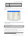
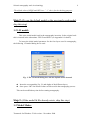
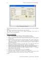
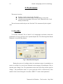
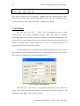
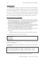
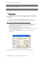
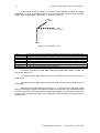
Seismic tomography tools
User Manual
For WINDOWS
By
Mohamed Farouk
and
Dapeng Zhao
Geodynamics Research Center
Ehime University
([email protected], [email protected])
July 2006
2
Seismic tomography tools in seismology
Index
Page
Contents
4
Tomotools Description ………………………….………………. 5
General strategy……………..……………………….………………. 5
How to install ? …………………………………..….……………….. 5
How to start ? ………………………………………………………… 5
Tomography tools …………………………………………………... 6
Tomography menu …………………….……………………….. 6
Tools menu ……………………………………………………… 6
Section menu ……………………………………………………. 6
Plot menu ………………………………………………………... 7
Step by step …………………………………………………………… 7
Tomography menu ……………………………………………… 7
Step 1 …………………………………………………….. 7
Control …………………………………………... 7
Step 2 ……………………………………………………. 9
1-D model ……………………………………….. 9
Step 3 ……………………………………………………. 9
Model Maker …………………………………… 9
Grid maker mode ………………………. 10
Grid reader mode ………………………. 10
How to construct a model1d file ……………….. 11
Step 4 ……………………………………………………. 11
Wintomo ………………………………………… 11
How to do tomography …………………………. 12
Tools menu ……………………………………………………… 14
ReadRes …………………………………………………. 14
How to read result? ………………………….…. 15
Poisson Ratio, Crack Density, Saturation Rate and 16
Porosity ………………………………………………….
How to calculate the tomography images of Poisson’s 16
ratio, Crack density, Saturation rate and Porosity? ….
Section Menu …………………………………………………... 18
Local/Tele Section ………………………………………. 18
How to construct a cross section………………... 19
Post data ………………………………………………… 20
How to construct a PostOut file ………….......... 21
Post events ………………………………………………. 22
How to construct a PostOut event file …………. 22
Ext_Section ……………………………………………… 23
How to extract data from a cross section and plot it on 23
the map ?…………….…………………………………..
Plot Menu ……………………………………………………….. 24
Surfer ……………………………………………………. 24
Preface …………………………….……………………………………
Tomotools for Windows – Trial version – July 2006
Seismic tomography tools in seismology
Tomotools limitations …………………………………….………...
Parameter limits of Tomotools
References ……………………………………………………………
Acknowledgments ………………………………..………………….
Appendix 1 User's Manual for TOMOG3D…………………………
Appendix 2 Input/Output formats………………………………......
Tomotools for Windows -Trial version – November 2004
3
25
25
27
28
29
41
4
Seismic tomography tools in seismology
Preface
Tomotools description
Tomotools is a Fortran-Quick win application to perform seismic tomography
images using Zhao (1992) code. The program consists of all the requirements of the
tomography inversion of P and S waves. Poisson ratio, Saturation rate, Crack density
and porosity tomography are also provided. The Model 1-D and grid net are
constructed easily by using the Model maker tool.
The construction of cross sections and the associated post files like volcanoes,
faults, events, etc, are all included.
The tomography results can be sent directly to a visual basic script to be
plotted by “SURFER (Golden software)”.
Tomotools preserves the original file formats (I/O) used in “Tomog3d“code
(Zhao, 1992). Therefore, the tomography tools in “Tomotools” can be applied directly
to the output results of the original code without any modifications.
Tomotools performs the tomography jobs in steps. The output of each step is
the input of the next. Starting from any step is allowed when the required files exist.
One of the most important features of Tomotools is the generality of the code.
It is valid for all grid numbers (in the allowed limits). The control parameters; input
and output file names and paths are inserted directly in the run time. The 1-D velocity
model can be changed in any step of the tomography job.
Tomotools is still in the development stage. I need your help to detect bugs
and errors to make it perfect. Sorry if any inconvenience resulted from this program.
Have a nice tomography.
Mohamed Farouk
[email protected]
[email protected]
Tomotools for Windows – Trial version – July 2006
Seismic tomography tools in seismology
General strategy
The general strategy of this manual is to explain how to perform a complete
tomography inversion using the different tools included in the Tomotools.
No need for any other codes or routines to perform the complete tomography
process. Tomotools constructs all helping file needed. The data file should be
provided by the user.
The purpose of this manual is not to describe the typical tomography
technique used in the code. Refer to Appendix 1 or Zhao (1992) for details.
The tomography images in this program are plotted through a visual basic
script in which all images will be plotted in Surfer program.
How to install?
Tomotools is a Quick win application that uses the windows library. It
does not need any registry or dynamic links (DLL) files. Copy the whole files into
the working directory and start to use.
How to start?
-Before start using this program read carefully the tomography technique of
Zhao (1992).
- Prepare the data in the exact format shown in the Appendices.
-Follow the step by step description shown below.
Tomotools for Windows -Trial version – November 2004
5
6
Seismic tomography tools in seismology
Tomography tools
The main window of Tomotools consists of several menus in which the different
tools are inserted. The tomography tools are classified into four menus:
1234-
Tomography
Tools
Section
Plot
1-“Tomography” menu
z
z
z
z
1-D model: To insert the initial model used in tomography.
Control: To insert or load the control parameters of the tomography process.
Model maker: To construct the “model 1D file” used in tomography process.
Wintomo: To perform tomography process for P or S wave.
2-“Tools” menu
z
z
z
z
z
Read Result: To convert the tomography output result into depth files to be
used for plotting.
Poisson Ratio: Construct a Poisson’s ratio tomography from P and S wave
tomography results.
Crack density: Construct a Crack density tomography from P and S wave
tomography results.
Saturation rate: Construct a Saturation rate tomography from P and S wave
tomography results.
Porosity: Construct a Porosity tomography from P and S wave tomography
result.
3-“Section” menu
z
z
z
z
z
Local Section: To construct vertical cross-sections from the Local
tomographic results.
Tele Section: To construct vertical cross-sections from the Teleseismic
tomographic results.
Post Data: Construct a “PostOut” file of data (Volcanoes, Faults, etc.) to be
overlaid on the cross section.
Post event: Construct a “PosOut” file of events to be overlaid on cross section.
EXT. Section: A specific tools for extracting anomalies from a section to
construct a model file.
Tomotools for Windows – Trial version – July 2006
Seismic tomography tools in seismology
4- “Plot“ menu
Consists of one submenu
z
Surfer: To open the surfer script where the complete tomography images are
to be plotted.
Step by step
The following section describes the above menus in steps.
1-Tomography menu:
Follow the next steps to perform tomography.
Step 1: (This step should be first done)
1-1 Control:
To insert the control parameters used in tomography. These parameters control
most of the tomography processes and should be inserted accurately. They are
inserted in the original tomography by using the “datacp file”. (See appendix for
detail)
These control parameters are as follows:
Parameter
NSTA
NEQS
NITLOC
RMSCUT
DVMAX
VDAMP
NHITCT
NITMAX
Description
Number of stations
Number of earthquakes
Maximum number of hypocenter relocations for each
iteration.
Cutoff value for event RMS residual to terminate relocation
in sec
Maximum velocity perturbation per iteration in km/s.
Damping factor for velocity
Minimum number of "observation" of a grid point for it to
be included in inversion
Maximum number of velocity inversion step.
Tomotools for Windows -Trial version – November 2004
7
8
Seismic tomography tools in seismology
RMSTOP
STEPL
TLIM
NITPB
Cutoff for overall RMS to terminate velocity inversion step.
Step length for accumulating velocity partials along ray
path.
Cutoff for travel time difference to terminate ray tracing in
sec.
Maximum permitted iterations for ray tracing
(See appendix for more details).
In Tomotools these parameters are inserted using the following “Control parameters”
dialog box
Fig. 1. Control parameters dialog box.
-The control parameters can be inserted directly into the dialog box or imported from
a “datacp file”. A “datacp file” should be in the same original format. Otherwise an
error message will appear.
A typical “datacp file” is as follows:
15305107 3 0.150 0.500 8.000
10 1 0.100 2.000 0.008 8
-The control parameters can be saved in a “datacp file” by using the “Export” button.
-The different parameters as given in the above table should be inserted accurately
according to the data used and the tomography conditions.
-The control dialog box entry is given in the tomography dialog box as a quick
checking or modifications for the different tomography trials.
N.C. -Especially the NSTA should be inserted as the exact number of stations exists in
the station file. Otherwise, a run time error will occur.
Tomotools for Windows – Trial version – July 2006
Seismic tomography tools in seismology
-The default value of NEQS and NSTA are ” -1” this is for the checking purpose.
Step 2: (To use the default model or the previously used model,
skip this step)
1-2 1-D model:
This is the initial model used in the tomography inversion. In the original code
this is inserted in the subroutines VEL1D and HLAY (see Appendix1 for detail).
To insert the initial model parameter for the four layers used in tomography,
the following 1-D model dialog box is used.
Fig. 2. The 1-D model dialog box with the default values inserted.
z
z
Insert the corresponding Vp, Vs and depths of the different layers.
Once press “OK” the inserted values will be used in the tomography process
This can be modified any time before starting tomography.
Step 3: (If the model1d file already exists, skip this step)
1-3 Model Maker
Tomotools for Windows -Trial version – November 2004
9
10
Seismic tomography tools in seismology
To construct the model1d file used in tomography. It does the same job as
“inidvp” routine. The model1d file is the same as that of the original tomography. It
consists of the following:
-Station list: The location of the stations used in tomography and labelled in the
arrival time data file. (See appendix for station file format)
-The gird nodes: The number and location of the horizontal and vertical grids used in
tomography. (See appendix for the grid nodes file format)
-The initial 3D model: The 3D initial values of velocities and perturbations of the
grid nodes used in tomography.
The “Model maker” Dialog box is used to receive the required information needed to
construct the model1d file. Unlike the original code, the grid nodes are constructed
here separately.
Fig. 3. Model maker dialog box.
Two modes of grid constructions are available.
z
Grid Maker mode: (when Grid maker is checked). In which the minimum and
maximum limits and interval of grids are inserted to automatically construct the
grid nodes. The depth grids are constructed according to the following relation:
G (I,J,K)= G(I,J,K-1) *(Interval)
Where G(I,J,K) is the grid node of Ith longitude and Jth latitude and Kth depth.
Tomotools for Windows – Trial version – July 2006
Seismic tomography tools in seismology
z
11
Grid Reader mode: (when Grid Reader is checked). In which an externally
edited grid file is directly used.
How to construct a model1d file?
z
z
z
z
z
Insert the file name of the station list used in the arrival time data.
Insert the file name of the output model1d file.
If using the grid maker mode, insert the minimum, maximum and intervals of the
latitude and longitude of the grid nodes in degree. Insert the interval of the depth
grids that give the suitable grids. The smaller values produce much number of
grids.
If using the grid reader, browse or edit a grid file with the same grid format in the
original model1d file (See appendix for detail).
Press “check” to see the grids inserted by either mode. Press accept to confirm
and construct the model1d file. Or, press “No” to repeat inserting grid parameters.
A typical example of a grid file is as follows:
29 35 10
GRIDS
29.08 34.90 34.93 34.96 34.99 35.02 35.05 35.08 35.11
35.14 35.17 35.20 35.23 35.26 35.29 35.32 35.35 35.38
35.41 35.44 35.47 35.50 35.53 35.56 35.59 35.62 35.65
35.68 40.16
113.92 136.70 136.73 136.76 136.79 136.82 136.85 136.88 136.91
136.94 136.97 137.00 137.03 137.06 137.09 137.12 137.15 137.18
137.21 137.24 137.27 137.30 137.33 137.36 137.39 137.42 137.45
137.48 137.51 137.54 137.57 137.60 137.63 137.66 154.91
-100.00 0.00 2.00 4.00 7.00 11.00 15.00 20.00 25.00
60.00
N.C.- When using the grid maker mode, after confirmation the grids will be written in
a grid file named ”tempgrid.txt”. This file can be used in grid reader mode for further
editing of the “grid maker” grids
-The maximum allowed number of grids are 99, 50 for the horizontal and vertical
direction, respectively.
Step 4 (Last step of tomography)
1-4 Wintomo
To start the tomography process using the “Control parameters” and the
“model1d “file previously constructed above. The tomography process is performed
through the following tomography dialog box.
Tomotools for Windows -Trial version – November 2004
12
Seismic tomography tools in seismology
Fig. 4. Tomography dialog box
The tomography dialog box consists of all the requirements needed in the tomography
routine.
The only new requirement in this dialog box is the “Data“file.
The “Data” file is the same as the original tomography code written in
“datala“ format. (See appendix 2).
How to do tomography?
1. Press “Control parameters” button if it still not loaded or inserted.
2. Press “1-D velocity model” to change 1-D velocity model if needed.
3. Browse or insert the model1d file constructed by this program or by the original
“inidvp” code.
4. Browse or insert the data file name specially prepared. This consists of the arrival
times of the different phases recorded by different stations and different
earthquakes. Number of events in this file should be greater or equal to NEQS in
the control parameters.
5. Browse or insert the “ResOut1” file name. This is an output file where the
tomography residuals are written when the “Verbose” is not checked.
6. Browse or insert the “ResOut2” file name. This is the output tomography file. It
consists of the velocity perturbations resulted from the tomography inversion.
7. Insert the first (IEQ1) and the last (IEQ2) earthquake to read. “-1” in “IEQ2”
means read all events in the file.
8. Check “P” or “S” for doing either “P” or “S” tomography.
9. Check/don’t check “Relocation” to relocate/not relocate events.
10. Check/don’t check “Verbose” to see/not see the residuals on the screen. If not
checked, the residuals will be written in the “ResOut1” file instead.
Finally,
Tomotools for Windows – Trial version – July 2006
Seismic tomography tools in seismology
13
11. Press “Start”.
¾ The message field will give messages resulted from the different tomography
routines. The error messages will be given in the message box.
¾ The progress rate of the tomography will be shown in the progress bar.
¾ When the tomography inversion ends, the important results will be shown in
the message list box
- The process can be repeated for several file names and several control parameters.
N.C: -The tomography process once started cannot be interrupted.
-The verbose mode makes the process too slow, it is recommended to uncheck the
verbose box.
-Do not modify the “ResOut2” file resulted from the tomography inversion. This
file is used for all the coming tools of plotting and cross sections.
-The output files are not protected against being replaced. Once “Start” is
pressed, all the output files will be replaced without warn.
Tomotools for Windows -Trial version – November 2004
14
Seismic tomography tools in seismology
2-Tools menu
This menu is used to:
z
z
z
Read the results written in the “ResOut2”
Construct cross sections and the corresponding overlay data.
Calculate the tomography of Poisson’s ratio, Saturation rate, Crack
density and Porosity.
The tools menu can directly use the “ResOut2” file constructed by the original
code.
2-1 ReadRes
To read the “ResOut2” file of either P or S tomography result then extracts the
perturbation of every grid layer into separated depth files The following Read Result
dialog box is used for this purpose.
Fig. 5. Read Result dialog box
During the process of reading results, the maximum range of perturbations to
extract is needed to be used in the limitation and averaging of perturbation. This is
inserted in the “Range” box. The perturbation values above this range will be equal to
“Range”. The perturbation value of a given grid node will be extracted only if the
number of hit count of this grid is less than “NHITCT” in the control parameter.
Tomotools for Windows – Trial version – July 2006
Seismic tomography tools in seismology
15
How to read result?
1.
2.
3.
4.
Browse or insert the “ResOut2” file name.
Insert the maximum perturbation range in the Range box.
Press “OK”.
If the “ResOut2” file is in the correct format, the following files will be
constructed:
1-Depth files:
A set of files consists of the perturbations of the grid nodes that have hit counts
more than “NHITCT”, one file for every depth layer is constructed.
Depth file name is the “ResOut2” name appended by “Dxxx” where “xxx is
the depth value of this layer and has the extension “dat”.
Ex: The file name of the grid layer 10 km of the file ResOut2 is “ResOut2D010.dat”
Format of the depth file is as follows:
First line: A string of depth value
Next lines: Each line consists of the longitude, latitude, perturbation, hit count
of the given grid.
A typical depth file is shown below:
20.0-KM
137.66 34.9 -1.916 0.05 100
137.66 34.93 0.454 0.01 83
137.66 34.96 0.354 0.01 69
137.66 34.99 0.194 0.01 60
137.66 35.02 0.194 0.01 53
137.66 35.05 0.164 0.01 24
137.66 35.08 0.174 0.01 17
137.66 35.11 0.184 0.01 11
137.66 35.14 0.194 0.01 10
2-Name-list file:
A “name-list” file consists of the number of files constructed and their names.
This is only used for the plotting purpose. This file is requested by the Surfer script to
read all the depth files and plot the tomography images simultaneously.
The “Name-list” file name will be of the same name of “ResOut2” file but has
the extension”NAM”.
Format of the “Name-list” file:
First line: Number of files
Tomotools for Windows -Trial version – November 2004
16
Seismic tomography tools in seismology
Next lines: Depth file names in order of increasing depth, as follows:
6
ResOut-15d20SD001.DAT
ResOut-15d20SD004.DAT
ResOut-15d20SD008.DAT
ResOut-15d20SD012.DAT
ResOut-15d20SD016.DAT
ResOut-15d20SD020.DAT
These files can be used independently in any other plotting software for gridding and
plotting the tomography images.
N.C. Don’t modify or change the format of the Name-list file. This file is used by the
surfer script included with this program to plot the tomography images.
2-2 Poisson Ratio, Crack Density, Saturation Rate and
Porosity
Calculate the tomography images of the above parameters from the P and S
wave tomography result. This is done by using the corresponding dialog box.
How to calculate the tomography images of Poisson’s ratio, Crack density,
Saturation rate and Porosity?
For Poisson’s Ratio:
1- Calculate the P and S wave tomography separately following the tomography
menu section.
2- Click the Poisson Ratio menu to open the Poisson Ratio dialog.
3- Browse or insert P-wave tomography Resout filename in the Resout-P box.
4- Browse or insert S-wave tomography Resout filename in the Resout-S box..
5- Browse or insert output Poisson’s ratio perturbation file in the Poisson box
6- Insert the suitable limit Range. This is the same as the range in the
tomography menu, not that of the cross sections. The default is 11.
7- Press “OK”.
-If the inserted filenames are accepted, the “Poisson” file will be generated and the
ReadRes routine will automatically called and generate the perturbation depth files
and the “name-list” files. (See ReadRes menu for detail).
Tomotools for Windows – Trial version – July 2006
Seismic tomography tools in seismology
Fig. 6. Poisson’s ratio dialog box.
For the calculation of the Saturation rate, Crack density and Porosity the above
steps are applicable for the corresponding menu.
N.C. -The range value differs from one parameter to another according to the
expected perturbation range.
-The resulted file of all these parameters are treated exactly the same as the Resout
data.
-The results of the above menu can be used in other programs for the purpose of
plotting.
Tomotools for Windows -Trial version – November 2004
17
18
Seismic tomography tools in seismology
3- Section Menu:
It is used to construct cross sections across the grid net used. The idea of this
menu is to use the “Blanking (BLN) file” of the “Surfer (Golden software)” for the
reading of the cross section coordinates. The BLN file is the basic of the digitized
map. Tomotools reads directly the BLN file as the digitization of the profile line
needed to be constructed.
Format of the “BLN ” file is as follows:
First line: Number of points, flag
Flag here is not important since it takes effect in “Surfer” only when the BLN
file represents a closed area, the flag in this case tells either to blank inside(0) or
outside(1) the area. From this the BLN file takes its name.
Next lines: longitude, latitude of the digitized point.
A typical “BLN” file is shown bellow:
12 1
136.5862012 36.4961662
136.68602365 36.2908408
136.80619825 36.0561832
136.94575585 35.8224718
137.0959741 35.5878142
137.18610505 35.3531566
137.3460148 35.090113
137.49623305 34.8554554
137.61640765 34.6700002
137.73658225 34.4164186
137.8267132 34.2593494
137.9061835 34.181761
- If the BLN file consists of 2 points delimiting the 2 limits of the cross section,
Tomotools will interpolate and fill points in between.
3-1 Local/Tele Cross Section
Both local and teleseismic tomography format is support. However, the
current version of TOMOTOOLS can only produce the local tomography results
(ResOut).
The cross section is constructed using the Cross Section dialog box (Fig. 7.).
Tomotools for Windows – Trial version – July 2006
Seismic tomography tools in seismology
19
Fig. 7. Cross Section dialog box
How to construct a cross section?
1- Digitize the cross section line by using “Surfer”. The “BLN” file of this line is
needed. Detailed digitization is to be made. Extrapolation between points does
not exit in this Tomotools version.
2- Click on the Cross section menu to open the Cross Section dialog box.
3- Insert or browse the BLN file name in the section file box.
4- Insert or browse the ResOut file name from which the perturbation is to be
extracted.
— In case of Local section (Local Section menu): ResOut file should be
resulted from tomotools.)
— In case of Tele section (Tele Section menu): ResOut file should be
resulted from Teletmg1 or Teletmg2 code (Zhao et al., 1994).
5- Insert or browse the output Cross section file name in the SecRes box.
6- Insert the range of perturbation to extract. (See ReadRes for detail)
7- Press “OK”
If the BLN file is accepted, the SecRes file will be constructed.
An example of the “SecRes” file is shown bellow
0.000
0.000
0.000
0.000
0.000
5.244
5.244
5.244
5.244
5.244
-1.000
-4.000
-8.000
-12.000
-16.000
-1.000
-4.000
-8.000
-12.000
-16.000
7.338
1.460
3.345
-0.794
0.374
6.393
0.186
2.803
-1.006
0.426
5.901
5.582
6.515
6.246
6.323
5.849
5.511
6.479
6.235
6.325
607
691
355
112
30
671
840
505
187
42
Tomotools for Windows -Trial version – November 2004
20
Seismic tomography tools in seismology
11.506 -1.000 5.653 5.810 729
11.506 -4.000 -1.941 5.393 1034
11.506 -8.000 1.880 6.419 711
Data in the SecRes file are in sequence: Distance from the starting point (in km),
depth (in km), perturbation extracted from the Resout file, 3D velocity and hit counts.
To plot the cross section, only the first three columns are required.
3-2 Post Data
The post file is an “X,Y” or BLN” file representing any type of data
overlaying the cross section tomography images. These data could be volcanoes
distribution, digitized maps like coast lines and faults or earthquake distribution. The
last one will be treated separately in the next section because it requires different (I/O)
formats. The depth value of all post data here is “zero”. It is supposed that they are
projected on the surface of the cross section.
The Post data menu is responsible for extracting the data from the post files
and rewrite in a format (PostOut) that can be overlaid directly on the cross section.
This is done by using the Post section dialog box (Fig. 8.)
Fig. 8. Post section dialog box
The limit of the cross section is an important parameter in the construction
process. This value represents the thickness of the cross section slice in degree. The
description of the Range value is shown in Fig.9.
Tomotools for Windows – Trial version – July 2006
Seismic tomography tools in seismology
21
Limit
A
Cross section
A’
Main map
Fig. 9. Schematic description of the “Limit” value.
How to construct a PostOut file?
1.
Digitize the cross section line by using “Surfer”. The “BLN” file of this line is
needed. Detailed digitization is to be made. Extrapolation between points does
not exit in this Tomotools version. (If this is already done, go to the next step.)
2. Click on the Post data menu to open the Post Section dialog box.
3. Insert or browse the BLN file name in the section file box.
4. Insert or browse the desired Post file from which the data is to be extracted to fit
in cross section. The post file can be either an “X,Y” or “BLN” data file.
If “X,Y” data: Data should be of two columns separated by a single space
representing the longitude and latitude, respectively.
If “BLN” data: A typical BLN format should be used.
5.
6.
Insert or browse the output PostOut file name in the PostOut box.
Insert the limit of extraction. In the case of faults use a small value (0.01) to
reduce the number of projected points.
7.
Press “OK”
If the BLN and post files are accepted, the SecOut file will be constructed.
An example of the “SecOut” file is shown bellow
Volcanoes
9.36 0.00
15.68 0.00
75.22 0.00
56.17 0.00
The data in this file is simply: The distance (in km) and depth. The depth of all
the “PostOut” files is Zero to be projected on the surface.
Tomotools for Windows -Trial version – November 2004
22
Seismic tomography tools in seismology
3-3 Post Events
This menu is the same as the “Post data menu” and uses the same dialog box.
It is used to overlay the earthquake distribution on the cross section in the actual depth
and scaled with magnitude value. It is separated here because the event file to read is
not an “X,Y” or a BLN file but a multi columns data. In addition, the “PostOut”
events do not have a zero depth. Here, this menu read the hypocenter parameters file
and rewrite in a PostOut file format that can be overlaid to the given cross section.
How to construct the event PostOut file?
1.
Digitize the cross section line by using “Surfer”. The “BLN” file of this line is
needed. Detailed digitization is to be made. Extrapolation between points does
not exit in this Tomotools version. (If this is already done, go to the next step.)
2. Click on the “Post events” menu to open the Post Section dialog box.
3. Insert or browse the BLN file name in the section file box.
4. Insert or browse the hypocentral parameter file from which the data is to be
extracted to fit in cross section. The typical example of the hypocentral parameter
file and its corresponding format is shown at the end of this section,
5. Insert or browse the output PostOut file name in the PostOut box.
6. Insert the Limit of extraction (in degree). All events away from the cross section
by the “limit” value will be extracted. (See the Post section above.)
7.
Press “OK”
If the BLN and post files are accepted, the “SecOut” file will be constructed.
An example of the event “SecOut” file is shown bellow
194.98 8.54 0.9
222.35 8.22 1.2
70.85 5.05 2.3
51.17 10.81 1.0
48.26 9.10 0.6
The data in the above example in sequence are as follows: Distance (km), event depth
(km) and event magnitude.
A typical example of the hypocentral parameter file used in the “Post events” menu is
shown bellow:
2 6 4
2 6 4
2 6 5
2 6 5
……….
3 58
22 30
3 10
10 0
54.39
26.25
45.16
34.38
0.06
0.09
0.08
0.06
35.155
35.290
35.029
35.297
0.14
0.24
0.19
0.22
137.989
138.150
136.961
137.836
0.15 -21.92 0.59 39
0.24 -40.12 0.81 41
0.25 -43.10 0.84 44
0.15 -2.73 1.35 41
0.3 0.00
0.6 0.00
1.0 0.00
1.4 0.00
The data descriptions of the above example in sequence are as follows:
Tomotools for Windows – Trial version – July 2006
Seismic tomography tools in seismology
23
IY,IM,ID,IH,IMIN,OSEC,DSEC,ELAT,DLAT,ELON,DLON,DEPTH,DDPS,NSTM,MAG,RMS
The writing formats are as follows:：
FORMAT(5I3,F7.2,F6.2,F8.3,F7.2,F10.3,2F7.2,F6.2,I4,f6.1,F6.2)
3-4 EXT. Section:
The EXT or (extracted) section is a special tool to extract data from a section
(X-Depth format) and convert it into a (Long-Lat-Depth format) to be projected on the
corresponding.
This tool is used for contouring a specific anomaly in a section to the
corresponding map. This is done through EXT section dialog box shown in fig. 10.
How to extract data from a cross section and plot it on the map?
1- Digitize the required anomaly from the section file in the form of BLN file
(X-depth). This can be done through the digitize tool in “SURFER”.
2- Open the EXT. Section dialog
3- Insert or browse the BLN file name in the “Section file” box.
4- Insert or browse the BLN file name of the data extracted from the section
(shown in 1) in the “Datasec” box.
5- Insert or browse the output file of the data extracted in the “Dataout” box.
6- Press “OK”
Fig. 10. EXT section dialog box.
If the input files are in the correct format the output file will be constructed.
Tomotools for Windows -Trial version – November 2004
24
Seismic tomography tools in seismology
4- Plot Menu
This menu is used for plotting the tomography results by using the “Basic
scripter” and the “Surfer application”.
The surfer application should be installed in the working machine before using
this tool.
4-1 Surfer
This menu links the Tomotools and the “Surfer scripter”.
How to plot ?
1- Click on the “Surfer” menu to open the Basic scripter. A dialog asking for
reading result will appear. If the “depth” and the “name-list” files are not
yet generated by ReadRes. Press “YES”.
2- The Basic scripter will start. Open the script file named “TOMOPLOT.BAS”. This is given with the Tomotools program. (It the script is
not automatically opened, open it from the Scripter)
3- Run the Script.
4- An “Open file” dialog box will appear. In this dialog box, open the “namelist” file which contains the depth files needed.
5- The procedure of plotting will start. When finish, the tomography images
of the depth files requested will be found plotted in the Surfer workspace.
Each image is labelled by its depth value.
Tips:
-
-Some problem may occur during reading file. Check the number of files
and the “dat” files being read.
-The plotting script can be improved by the user.
The file “color3.lvl” is the color scale used to plot the images. It can be
modified according to the limits of the perturbation. It should be in the
same working directory of the data being read.
Tomotools for Windows – Trial version – July 2006
Seismic tomography tools in seismology
25
Tomotools limitations:
Maximum number of horizontal grids
Maximum number of depth grids
Maximum number Cross section line
Maximum number of event
Maximum number of stations
Tomography process
Memory
99
50
1000
6000
1600
Can not be interrupted
Reserve memory for the maximum
limits of dimensions.
Parameter limits of Tomotools:
PARAMETER (MD =120000,MU =180000,MG =120000*80)
PARAMETER (MEQ =6000 ,MST=1600 ,MAX=1000,MDT=2000)
PARAMETER (MKA =12001 ,MPA=99
,MRA=99 ,MHA=50)
PARAMETER (MSEC=1000)
All the above variables are employed similar to the original tomography (see
appendix1) except MSEC which is the maximum number of points in the cross
section.
____________________________________________________
Last updates: Jan 2007
Tomotools for Windows -Trial version – November 2004
26
Seismic tomography tools in seismology
Notice
This program is still under development and the author is
not responsible for any inconvenience for invalid results
produced by this program.
For more explanation about this program contact me.
[email protected]
Tomotools for Windows – Trial version – July 2006
Seismic tomography tools in seismology
27
Reference:
Abdelwahed, M. F., 2006. Waveform modeling and tomographic imaging in Japan
Islands. P.hD. Thesis. Geodynamics Research Center, Ehime University, Japan.
Zhao, D. Hasegawa, A., Horiuchi, S. 1992. Tomography imaging of P and S wave
velocity structure beneath northeastern Japan. J. Geophys. Res. 97, 19909-19928.
Zhao, D., Hasegawa, A., Kanamori, H., 1994. Deep structure of Japan subduction
zone as derived from local, regional and teleseismic events. J. Geophys. Res., 99,
22313-22329.
Tomotools for Windows -Trial version – November 2004
28
Seismic tomography tools in seismology
Acknowledgments:
Great thanks and appreciation to Dapeng Zhao for his
permission to use his tomography code in this application.
Many thanks to all the GRC members (Eqlab in special)
for their help. Ehime University with the supervision of
Dapeng Zhao provides all the facility to establish this
program.
Tomotools for Windows – Trial version – July 2006
Seismic tomography tools in seismology
29
Appendix 1
User's Manual for TOMOG3D
Written by :
Prof. Dapeng Zhao
Seismological Laboratory 252-21, California Institute of Technology
Pasadena, CA 91125, U.S.A.
June 25, 1994
I wrote this manual when I was in Japan in 1989 for the initial version of my
tomography program for local (and regional) earthquake tomography. Since then I
have modified the code considerably, e.g., the inversion part is replaced by the
LSQR algorithm, the addition of the teleseismic inversion etc. But the basic parts, like
the grid setting, the treatment of discontinuities and later phases, and 3-D ray tracing
are basically the same. I will try to write an updated version of the manual for the
newest version of my tomography program for the joint inversion of local, regional
and teleseismic event data.
_____________________________________________________
Observation Center for Prediction of
Earthquakes and Volcanic Eruptions
Faculty of Science, Tohoku University, Sendai 980, Japan
April 30, 1990
Now,
Geodynamics Research Center (GRC)
Ehime University, Japan
INTRODUCTION
The computer algorithm TOMOG3D, written in FORTRAN 77, is designed to
use arrival time data from local earthquakes recorded by a network of seismic
stations to derive a 3-D seismic velocity model for the crust (and the upper mantle)
beneath the network. The conceptual approach parallels the conventional
tomography method, being composed of the following steps as clearly shown in main
part of the program,
(1) Initialization (call subroutine STAT);
(2) Input
z
z
z
Control parameter (call INPUT1),
Station list (INPUT2),
Initial velocity model (INPUT3),
Tomotools for Windows -Trial version – November 2004
30
Seismic tomography tools in seismology
z
Initial hypocentral locations and arrival time data (INPUT4)
(3) For every earthquakes, first relocate the hypocenter (LOCEQK), then
calculate derivatives of travel times with respect to hypocentral
parameters and medium parameters (FORWRD);
(4) Invert for velocity model adjustments (VELADJ) and output the inverted
velocity model (OUTADJ).
Thus, one iteration is accomplished. From the travel time residual reduction
through the iteration, decide if or not to perform the next iteration.
Code Advantages:
Albeit its similarity to previous algorithms, TOMOG3D has several outstanding
advantages.
z
z
z
z
-Firstly, it adopts a quite realistic model that several complicated velocity
discontinuities (CVDs) exist and velocities between these CVDs have
variations in three-dimension.
-Secondly, it contains a robust and efficient 3-D ray tracing technique to
calculate travel times and ray paths in such a complex model.
-Thirdly, just because of the above two features, in addition to first P and
S waves TOMOG3D can combine arrival time data of later phases, i.e.,
waves converted or reflected at the CVDs, important information but
being completely thrown away in previous 3-D studies.
-Finally, unlike Thurber's SIMUL3 which can only work for arrays
extending smaller than 50-km by 50-km, TOMOG3D is expected to
perform well for regions with size from several hundred meters to several
thousand kilometers, partly due to the spherical coordinates system it
used.
Because of these advantages, TOMOG3D is considered to be powerful in the
3-D studies in regions such as subduction zones, fault zones and continent regions
with large depth variations of the Conrad and the Moho discontinuities.
TOMOG3D is a complex and completely self-contained algorithm, including
one main program and 52 subroutines, and requiring 85 kbyte of memory storage.
Many (small) tricks are adopted in some subroutines, which may be not so easy to
understand. In the following illustration, I mainly explain the meanings of the
variables (scalar, vector or matrix) and some tricks that I used. The role of a
subroutine played is usually given as comments inserted in the subroutine and will
not be repeated here.
PROGRAM INPUT
(1) Control File (subroutine INPUT1)
Common block:
$
$
&
COMMON/CONTRL/NSTS,NEQS,NOBT,NITLOC,RMSCUT,DVMAX,VDAMP,
NHITCT,NITMAX,RMSTOP,STEPL,XFAC,TLIM,NITPB
Zhao et al.(1989)
Tomotools for Windows – Trial version – July 2006
Seismic tomography tools in seismology
Parameter
NSTS
NEQS
NOBT
NITLOC
Format
I4
I4
RMSCUT
F7.3
DVMAX
VDAMP
NHITCT
F7.3
F7.3
I4
NITMAX
RMSTOP
I4
F7.3
STEPL
F7.3
XFAC
F7.3
TLIM
F7.3
NITPB
F7.3
I4
31
Description
Number of stations +
Number of earthquakes
Total number of data *
(3) Maximum number of hypocenter relocations at each
iteration.
(0.15) (SEC) Cutoff value for event rms residual to
terminate relocation.
(0.5) (KM/S) Maximum velocity perturbation per iteration.
(5.0) Damping factor for velocity
(20) Minimum number of "observation" of a grid point for it
to be
included in inversion
(3) Maximum number of velocity inversion step.
(0.15 Sec) Cutoff for overall rms to terminate velocity
inversion step
(5.0 KM) Step length for accumulating velocity partials
along ray path, only presents in subroutine TTMDER.
(1.0) Convergence enhancement factor for pseudobending.
(0.002 Sec) Cutoff for travel time difference to terminate
ray tracing.
(8) Maximum permitted iterations for ray tracing
+ Effectively 60 stations are used.
* Note that in control file only NOBT is not inputted one. NOBT is accumulated in
subroutine PARSEP
----------------------------------------------------------------------------------------------------------------2) Station list (subroutine INPUT2)
Common block:
$ COMMON/STATIN/PHIS(MST),RAMS(MST),HIGS(MST),STC(3,MST) $
Variable
PHIS(N)
RAMS(N)
HIGS(N)
STC(1,N)
STC(2,N)
STC(3,N)
Explanation
Latitude of N-th station, in degree
Longitude of N-th station, in degree
Elevation of N-th station, in kilometer
Colatitude of N-th station, in radian
longitude of N-th station, in radian
-HIGS(N)
Note that only STC(I,N),(I=1,2,3) is used in calculation.
(3) Initial velocity model (subroutine INPUT3)
Common block:
$
$
$
$
$
$
$
$
COMMON/VMOD3D/NPA,NRA,NHA,PNA(MPA),RNA(MRA),HNA(MHA),
&
VELAP(MPA,MRA,MHA),VELAS(MPA,MRA,MHA),
&
NPB,NRB,NHB,PNB(MPB),RNB(MRB),HNB(MHB),
&
VELBP(MPB,MRB,MHB),VELBS(MPB,MRB,MHB),
&
NPC,NRC,NHC,PNC(MPC),RNC(MRC),HNC(MHC),
&
VELCP(MPC,MRC,MHC),VELCS(MPC,MRC,MHC),
&
NPD,NRD,NHD,PND(MPD),RND(MRD),HND(MHD),
&
VELDP(MPD,MRD,MHD),VELDS(MPD,MRD,MHD)
Tomotools for Windows -Trial version – November 2004
32
Seismic tomography tools in seismology
In the names of these variables, P, R and H mean latitude, longitude and depth,
respectively. A, B, C, D denote four layers, here the upper crust, the lower crust, the upper
mantle and the Pacific plate, respectively. P, P-wave; S, S-wave.
North
P-axis (latitude)
West
R-axis (longitude)
Grid point
Depth
Figure 1. The coordinates system.
NPA
NRA
NHA
PNA(I)
RNA(J)
HNA(K)
VELAP(I,J,K)
VELAS(I,J,K)
The number of column of grid meshes in latitude direction for layer A; the upper crust;
The number of column of grid meshes in longitude direction for layer A; the upper crust;
The number of layers of grid meshes in depth direction for layer A; the upper crust;
The latitude of I-th row of grid points in layer A;
The longitude of J-th column of grid points in layer A;
The depth of K-th layer of grid points in layer A;
P-wave velocity at the grid point (I,J,K) in layer A
S-wave velocity at the grid point (I,J,K) in layer A
The same convention for NPB, NRB, NHB, PNB, RNB, HNB, VELBP, VELBS
layer B, the lower crust;
for
The same for NPC, NRC, NHC, PNC, RNC, HNC, VELCP, VELCS for layer C, the
upper mantle;
The same for NPD, NRD, NHD, PND, RND, HND, VELDP, VELDS for layer D, the
Pacific plate.
Note that (see file DATATMG1) here NHC=7, i.e., 7 layers are set in the upper mantle.
But only the internal 5 layers of grid points are taken to be unknowns, the uppermost and the
lowermost layers are only used to perform velocity interpolating. The same for the upper crust,
the lower crust and the Pacific plate. The configuration of the grid mesh in depth direction is
shown in Fig.2.
Tomotools for Windows – Trial version – July 2006
Seismic tomography tools in seismology
33
Surface
la
ye
rs
.
Layer A
ab
ov
e
Conrad
f ro
m
th
e
Layer B
Moho
po
la
tio
n,
an
d
is
lic
a
te
d
fo
r
aw
a
y
Slab
fo
rv
el
oc
it
y
in
te
r
Layer C
la
ye
ri
s
us
ed
Layer D
Th
is
Grid node
Figure2. Velocity model.
Here NPC=23, NRC=13, i.e., 23 rows and 13 columns of grid points are set in the
latitude and longitude directions, respectively, for the upper mantle. However, the same as in
the depth direction, only the internal (23-2)*(13-2) grid points are taken to be unknowns for
each layer, the outer ring of the grid points are used only to interpolate velocities at points
between the outer ring and the internal grid points.
Thus the total number of grid points which are taken to be unknowns is
NODETOT
=
(NPA-2)*(NRA-2)*(NHA-2)
+
(NPB-2)*(NRB-2)*(NHB-2)
+ (NPC-2)*(NRC-2)*(NHC-2) + (NPD-2)*(NRD-2)*(NHD-2)
User must be careful that for each layer (the upper crust, lower crust etc.) the
uppermost and lowermost mesh layers and the outer ring of grid points for each mesh layer
should be located far away from the internal grid points so that all the ray paths are located
within the modelling grid mesh space. An example of setting grid meshes is shown in file
DATATMG1 which is used for an application to Tohoku district, NE Japan.
$
$
$
$
COMMON/V0ABCD/VINAP(MPA,MRA,MHA),VINAS(MPA,MRA,MHA),
&
VINBP(MPB,MRB,MHB),VINBS(MPB,MRB,MHB),
&
VINCP(MPC,MRC,MHC),VINCS(MPC,MRC,MHC),
&
VINDP(MPD,MRD,MHD),VINDS(MPD,MRD,MHD)
This common block of variables are used to store initial P and S wave velocities at
grid points set in layers A, B, C and D.
(4) Arrival time data (subroutine INPUT4)
Common block:
$
$
$
COMMON/STODAT/IYMSTO(MEQ),IDSTO(MEQ),IHRSTO(MEQ)
COMMON/EVENTS/MINO(MEQ),SECO(MEQ),PHIE(MEQ),RAME(MEQ),
&
DEPE(MEQ),EVC(3,MEQ),KOBS(MEQ)
Variable
IY
IM
ID
IH
IMIN
Format
I2
I2
I2
I2
I2
Description
year of an earthquake
Month
Day
Hour
Minute
Tomotools for Windows -Trial version – November 2004
34
Seismic tomography tools in seismology
SECO(N)
DT
PHIE(N)
DPHI
RAME(N)
DRAM
DEPE(N)
DDEP
NSTM
FMG
RMS
F6.2
F5.2
F7.3
F6.3
F8.3
F6.3
F6.2
F5.2
I3
F4.1
F5.2
Variable
YMSTO(I)
IDSTO(I)
IHRSTO(I)
MINO(I)
EVC(1,I)
EVC(2,I)
EVC(3,I)
Format
I4
I2
I2
I2
NSTN(J) I3
TT(J)
F6.2
IKPS(J) I2
Second
standard error of SECO(N)
latitude in degree
error of PHIE(N) in deg.
longitude in deg.
error of RAME(N) in deg.
focal depth in km
error of DEPE(N) in km
number of all data for i-th event
Magnitude
rms travel time residual of the
second
hypocentral location, in
Description
year and month of i-th earthquake
Day of i-th earthquake
Hour of i-th earthquake
Minute of i-th earthquake
(radian) colatitude of i-th earthquake
(radian) longitude of i-th earthquake
(Km)
focal depth of i-th earthquake
station number, denoting the station which recorded the datum
datum, arrival time of a seismic wave
wave type of the datum, which was identified by the user when he
collects data from seismograms,
1, first P-wave *
2, first S-wave
3, PS-wave converted at UBPP
4, SP-WAVE converted at UBPP
5, SmP-wave converted at the Moho
6, P*-wave refracted at the Conrad
7, Pn-wave refracted at the Moho
8, unknown wave which may be Pg,P* or Pn
--------------------------------------------------------------------UBPP: the Upper Boundary of the Pacific Plate
* Note that for crust event (dep.le.30km) the first arrival is Pg wave when epicentral distance
(DEL) is smaller than about 90km, and IKPS=1. The first is P* when DEL is from 100-135km,
then IKPS=6.When DEL is larger than about 140-150km, the first is Pn-wave, and
IKPS=7.
If you can not decide the wave type, please just take IKPS to be 8. For deep event
(DEP.gt.50km) IKPS=1 for first P arrival and IKPS=2 for first S arrival.
Common block:
$
COMMON/OBSERV/ISTO(MST,MEQ),SECT(MST,MEQ),KWV(MST,MEQ),
$
&
ISTO
SECT
KWV
WT(MST,MEQ),W(MST)
$
$
station number
arrival time of wave (data)
wave type
Tomotools for Windows – Trial version – July 2006
Seismic tomography tools in seismology
35
WT
weight
W
weight
---------------------------------------------------------File DATATMG2, which contain arrival time data of several events, is provided for reference.
MODELLING
(1) Velocity discontinuities
Subroutine HLAY(P,R,H,IJK)
The depth distributions of the Conrad, the Moho and the upper boundary of the
Pacific plate are represented by power series of latitude and longitude centred at (38.5,140.5).
The power series are calculated by subroutine DEPFUN(PW,RW,CG,ICM), and the output is
CG(N), the corresponding coefficients are given by CFAH in HLAY. CFAH(1)- CFAH(28) are
for the Conrad depth, CFAH(29)-CFAH(49) are for the Moho depth, and CFAH(50)-CFAH(77)
are for the UBPP depth. The coefficients from CFAH(1) to CFAH(49) are obtained by inverting
arrival time data from shallow events by Zhao et al.(1990), whereas those from CFAH(50) to
CFAH(77) are obtained by Dapeng Zhao from representing in power series the result of
Hasegawa et al.(1983).
(2) 3-D map of grid mesh
Giving a point Q in the modelling space, firstly we must know which are the eight
grid points surrounding Q, i.e., we must find the coordinates of A1, A2, A3,......,A8 as
shown in Fig.3.
A4
A2
A1
A3
Q
A6
A5
A8
A7
Figure 3. Eight grid points surrounding Q.
These coordinates can be represented by three parameters, IP, JP, KP. Assuming Q
is located in Layer C (the upper mantle), for convenience, IP, index of grid point in latitude
direction, IP=1 for the southmost grid, IP=NPC for northmost grid;
JP, index of grid point in longitude direction, JP=1 for the westmost grid, JP=NRC for
eastmost grid;
KP, index of grid point in depth direction, KP=1 for the uppermost grid, KP=NHC for
lowermost grid;
Let's define
Tomotools for Windows -Trial version – November 2004
36
Seismic tomography tools in seismology
IP1 = IP+1
JP1 = JP+1
KP1 = KP+1
So the coordinates of the eight points surrounding Q can be written as
A1(IP,JP,KP) ,
A2(IP1,JP,KP) ,
A3(IP,JP1,KP) ,
A4(IP1,JP1,KP),
A5(IP,JP,KP1)
A6(IP1,JP,KP1)
A7(IP,JP1,KP1)
A8(IP1,JP1,KP1)
For a point Q(P,R,H), IP,JP,KP can be found from subroutines VEL3 and VABPS, which
need calling subroutines BLDMAP, PRHF and INTMAP. In BLDMAP, the modelling space is
further subdivided in step length of 0.01 degree in latitude and longitude directions and 1 km
in depth direction.
As shown in subroutine VABPS, velocity at Q is obtained from interpolating the velocities at
A1, A2,.....A8, and can be written as
VQ = VA1*WH(1)+VA2*WH(2)+.....+ VAi*WH(i) + ....+ VA8*WH(8),
where VAi is velocity at grid Ai around Q, WH(i) is the distant weight. The nearer to Ai the
point Q is, the larger WH(i) is. The value of WH(i) is always in the interval [0,1].
Similar to velocity, components of velocity gradient dV/dP, dV/dR and dV/dH in three direction
(P,R,H) can also be obtained, as shown in subroutine VELD.
RAY TRACING
Subroutine TRAVT
INPUT
PE
Colatitude of hypocenter, in radian
RE
Longitude of hypocenter, in radian
HE
Focal depth of hypocenter, in km
PS
Colatitude of station, in radian
RS
Longitude of station, in radian
HS
Depth of station from sea level, in km
XFAC Enhancement factor for pseudo-bending
TACC Cutoff for travel time difference to terminate iteration
NITPB Maximum permitted iteration for ray tracing
PO
Observed travel time
OUTPUT
DEL
Epicentral distance, in km
VE
velocity at hypocenter, in km/s
FST
Fastest travel time
NRP
Number of points which define the final ray path
RP
Coordinates of the points in the ray path
RP(1,i): colatitude of i-th point, in radian
RP(2,i): longitude of i-th point, in radian
RP(3,i): Depth of i-th point, in km. Note that the first point, i=1, is at station; the
final point, i=NRP, is at the hypocenter.
IVK(i)
Denote which layer the i-th point is in, 1,2,3,4 correspond to the
upper crust, the lower crust, the upper mantle and the Pacific plate.
IWK(i)
Order(JUNBAN, in Japanese) of the segment which includes the i-th point.
The ray between two adjacent discontinuities is called "segment" here. See below for detail.
Tomotools for Windows – Trial version – July 2006
Seismic tomography tools in seismology
37
Segment of ray
KPS
1P
2S
3 PS
4 SP
5
6 P*
7 Pn
8 Pu+
1
1
2
2
1
1
1
1
1
2
1
2
2
1
1
1
1
1
3
1
2
2
1
2
1
1
1
4
1
2
1
2
2
1
1
1
5
1
2
1
2
2
1
1
1
Figure 4. IWV(8,5). KPS, wave type.
+ Pu, unknown wave type, may be Pg, P* or Pn.
Matrix IWV(8,5), as given in DATA statement in subroutine TRAVT, is shown in Figure 4. The
row denotes the wave type KPS (1,2,...,8), the column denotes the segment number in a ray
path. IWV(KPS,IWK(I)) denotes the wave kind, P or S wave, of I-th point in the ray path. The
wave type KPS of the ray is assigned by the user in the data set (common block OBSERV).
For example, for PS wave which converted at UBPP, KPS=3.
(1) When the hypocenter of a deep earthquake is within the Pacific plate, there are four
segments in the ray path. The first (IWK(i)=1) is in the upper crust(Lay 1),the
second(IWK(i)=2) is in the lower crust(Lay 2), the third (IWK(i)=3) in the upper mantle (Lay 3),
and the fourth(IWK(i)=4) in the Pacific plate(Lay 4). So the wave kind of PS wave at the four
segments is 2,2,2,1. (1, P-wave; 2, S-wave).
(2) when the hypocenter of a deep earthquake is located slightly above the Pacific plate and
the epicentral distance is so large that the wave refracted at UBBP is the first arrival, there are
five segments in the ray path, the former four ones are in Layers 1,2,3 and 4, respectively, the
fifth segment (IWK(i)=5) (one of its ends is hypocenter) is in the upper mantle (Layer 3) again.
The wave kind for the five segments is 2,2,2,1,1.
For Pn-wave, KPS=7, (1) when hypocenter is in the upper crust, there are five segments, in
Layers 1,2,3,2,1, respectively. The wave kinds for the five segments are all 1 (P-wave).
(2) When hypocenter is in the lower crust, there are four segments, in Layers 1,2,3,2,
respectively. The wave kinds are all 1 (P-wave).
(PG,RG,HG,VG), (PA,RA,HA,VA), (P,R,H,V) are middle variables, denote the colatitudes,
longitudes, depths and velocities at the points in every segments of the ray path.
NS(5), NSA(5), number of points in each of the segments of the ray path.
IV(i), IVA(i),(i=1,2,..5), denote which layer the i-th segment is in. IH(i), IHA(i),(i=1,2,..5), order
(JUNBAN, in Japanese) of segment in the ray path.
R0, radius of the earth, taken to b earthquake e 6371.05km here.
PIDEG, pi degree, equal to 3.14159265/180.0 = 0.017453.
EPS, a small positive value, being used to prevent zero to be quotient
LAY, the layer the hypocenter is in,
1,
2,
3,
4,
the upper crust;
the lower crust;
the upper mantle;
the Pacific plate.
Tomotools for Windows -Trial version – November 2004
38
Seismic tomography tools in seismology
IHEAD head wave (refracted wave) or not,
1, yes, may be P* (refracted at the Conrad), Pn ( at the Moho) or at UBPP, when the
hypocenter is located slightly above UBPP and the hypocentral distance is relative large, e.g.,
farther than 400 km.
0, no.
Subroutine BEND
Note that for ray segments in the upper and the lower crust (IV.LE.2) we do not perform
pseudo-bending, i.e., we assume the two segments to be straight line. This approximation is
confirmed to be good with error of smaller than 0.01sec because the lengths of the segments
in the upper and the lower crust are only about several tens of kilometers and the velocity
perturbation is about 6-7% for P-wave, and about 10% for S-wave.
If you also want to perform pseudo-bending for ray segments in the upper and the lower crust,
lease just remove the statement,
" IF(IV.LE.2) RETURN "
and do a little modification in subroutine MINIMUM.
Subroutine LENGTH
In TOMOG3D, this subroutine is one of the work-horses, so we want to find a simple
expression for DS, the spatial distance between two points in the earth's interior.
Define
PES = PE-PS,
RES = RE-RS,
PES2 = (PE+PS)/2.0,
The epicentral distance(DEL) in radian between (PE,RE,HE) and (PS,RS,HS) can be written
as:
DEL = SQRT( PES*PES + RES*RES* SIN(PES2)*SIN(PES2) )
According to Bullen & Bolt (at Page 232 in "An introduction to the theory of seismology",
fourth edition, 1985 ), and the error of this formula is less than 1 km if DEL is not longer than
6.5 degree.
Then using cosine formula, and cos(DEL) = 1-2*sin(DEL/2)*sin(DEL/2), and the approximate
relation, sin(DEL/2) = DEL/2 when DEL is small, the simple expression for DS is obtained.
TRAVEL TIME DERIVATIVES
Subroutine TTMDER
When KOPT = 0, calculate DTH(MST,4), travel time derivatives with respect to hypocentral
parameters;
When KOPT = 1, calculate DTM(MGO), travel time derivatives with respect to medium
parameters.
Note that the medium parameters are the velocity perturbation at every grid points, dV/V,
which are arranged as the following,
Tomotools for Windows – Trial version – July 2006
Seismic tomography tools in seismology
39
(dVap/Vap, dVas/Vas, dVbp/Vbp, dVbs/Vbs,dVcp/Vcp, dVcs/Vcs, dVdp/Vdp, dVds/Vds)
a,b,c,d denote the four layers, the upper crust, the lower crust, the upper mantle and the
Pacific plate;
p, s, P-wave, S-wave.
Subroutine NODO
Seeing Fig.3 and considering the following six cases, for convenience we assume Q is in the
upper mantle,
(1) when KP=1, i.e., Q is located just beneath the uppermost mesh the grids
A1,A2,A3,A4 are ones not included in velocity inversion but just for velocity
interpolation, so travel time derivatives
with respect to the velocities at these
grids are not necessary, so we call them "unnecessary grids (UNGs)";
(2) when KP=NHC1, i.e., Q is located just above the lowermost mesh layer, the
UNGs are A5,A6,A7,A8;
(3) when JP=1,i.e., Q is located just east of the westmost column of grids,
A1,A2,A5,A6 are UNGs;
(4) when JP=NRC1,i.e., Q is located just west of the eastmost column of grids,
A3,A4,A7,A8 are UNGs;
(5) when IP=1,i.e., Q is located just north of the southmost row of grids, A1,A3,A5,A7
are UNGs;
(6) when IP=NPC1,i.e., Q is located just south of the northmost column of grids,
A2,A4,A6,A8 are UNGs.
(7) Through NODO, picked out are UNGs, travel time derivatives with respect to
velocity perturbations at which are not needed.
VELOCITY INVERSION
Subroutine VELADJ
For a velocity model which is represented by grid points, there are usually many grids which
are not hitted by rays. Therefore velocity perturbations at these grids can not be resolved, and
had better be removed from the unknown vector to reduce burdens of memory storage and
inversion operations. To do this, we can reorder the unknown vector from the hit count record
of every grids, KHIT. Two vectors INDEX and JNDEX are used to accomplish this work.
Suppose the initial unknown vector is RHSINI, the dimension is NODETOT, all grids except
those at the outermost edge of the model, and the final unknown vector is RHSFIN, the
dimension is MBL, the number of grids hitted by rays of at least NHITCT.
If velocity perturbation at a grid, say A, is the i-th element in RHSINI, and is the j-th element in
RHSFIN, then we have the relation,
J = INDEX(I)
Oppositely, if we know the velocity perturbation at A is the j-th element in RHSFIN, and we
want to know which element (I-th) the velocity perturbation at Q is in RHSINI, we use the
relation,
I = JNDEX(J)
Using INDEX and JNDEX, we reorder the unknown vector RHS and derivative matrix G, and
perform inversion, then apply inverted velocity perturbation to the original model. This is the
algorithm of VELADJ.
Tomotools for Windows -Trial version – November 2004
40
Seismic tomography tools in seismology
Finally, let's pay attention to the dimensions of some important matrices.
In TOMOG3D, we assign MST=90. Note that MST is not number of stations but is maximum
number of data for a event, i.e., the sum of first P and S wave data and all the later phases
data for the event which have the largest number of data among all events in the data set. If a
study use only first P-wave or S-wave, then MST can be taken to be equal to the number of
stations.
MGD is number of all the grid points, MGD=NODETOT.
MGO = MGD*MST
Here I assign MG2 = 3830*(3830+1)/2, it seems MG2=MGD*(MGD+1)/2. In fact MG2 should
be written as
MG2 = MBL*(MBL+1)/2
For saving memory storage. MBL is the number of grids hitted by rays of at least the
threshold, NHITCT. Note that G(MG2) is the largest array in TOMOG3D, and occupy a large
part of the program size.
SOME REMARKS
The program shown here is just the first version of TOMOG3D, some extensions or
improvements can be easily made in the following respects.
1.
2.
3.
4.
The depth distributions of discontinuities are fixed during velocity inversion here.
They can also be included to be unknowns if sufficient data, especially those of later
phases are available.
Here the depth distributions of discontinuities are expressed by power series of
latitude and longitude, i.e., continuous functions. They can also be expressed by
grid meshes, just like velocity.
The inversion method used here is the standard damping least square method. This
method will fail to work when the number of unknowns is very large, e.g., more than
4000. In that case CG-type or ART-type inversion method should be used.
Usually the calculation of resolution kernel and standard error for one grid point is
the same as one iteration of velocity inversion, and the calculation for all grids
seems impossible and unnecessary when the number of unknowns is large, e.g.,
more than 2000. In this case, the pulse response technique can be used to
calculate the resolution kernel, and the Jack knife technique can be used to
calculate the standard error.
The author is performing the extension of TOMOG3D by taking into account that
mentioned above, and will present in later edition a new version of TOMOG3D, which is
expected to be more robust and efficient.
As mentioned in INTRODUCTION, TOMOG3D is a complex program, including more
than 50 subroutines. The author doesn’t think the program is a perfect one. There may exist
other techniques and approaches which can make some subroutines more efficient. The
author strongly advises that all users generate appropriate test cases, modelled on the actual
data sets to be analyzed to confirm that TOMOG3D will perform adequately when applied to
the actual data.
Thank you for your interest in my TOMOG3D.
Good luck on your seismic tomography!
Tomotools for Windows – Trial version – July 2006
Seismic tomography tools in seismology
41
Appendix 2
Input/Output formats
For the purpose of windows programming and better treating data, little changes are
done in data format reading.
The comparison between the old and the now format are given below
Subroutine
Tomogla
Tomotools
INNPUT3
140 FORMAT(5(11F5.2/))
140 FORMAT(5(11F6.2/))
Subroutine
Tomogla
Tomotools
INNPUT4
100 FORMAT(5I2,F6.2,F5.2,F7.3,F6.2,F9.3,2F6.2,F5.2,I3,F4.1,F5.2)
100 FORMAT(5I2,F6.2,F5.2,F7.3,F6.2,F9.3,2F6.2,F5.2,I4,F4.1,F5.2)
Data file:
2 6 4 1 9 28.00 0.02 35.984 0.09 137.566 0.12 5.74 0.37 21 0.2 0.00
471 29.15 0 1 0 471 29.85 0 2 0 465 29.92 0 1 0 465 31.12 0 2 0
392 33.48 0 1 0 392 37.02 0 2 0 474 37.10 0 2 0 135 34.33 0 1 0
1202 34.68 0 1 01202 39.19 0 2 0 470 39.43 0 2 0 498 35.05 0 1 0
498 39.65 0 2 01230 36.03 0 1 01230 41.38 0 2 0 119 41.61 0 2 0
152 37.47 0 1 0 152 43.64 0 2 0 478 38.06 0 1 0 478 44.91 0 2 0
508 39.60 0 1 0 0 0.00 0 0 0 0 0.00 0 0 0 0 0.00 0 0 0
2 6 4 151 5.46 0.05 35.860 0.13 137.547 0.30 7.10 0.64 14 0.0 0.00
1st line is the same as the hypocentral parameter file in cross section tools as follows:
IY,IM,ID,IH,IMIN,OSEC,DSEC,ELAT,DLAT,ELON,DLON,DEPTH,DDPS,NSTM,MAG,RMS
Where: IY,IM, ID: year, month, day of the earthquake.
IH,IMIN, Osec, DSEC: Hour, Min, Sec of origin time, error in origin time.
Elat, Dlat: Latitude of earthquake in degree, error in lat.
Elon, Dlon: Longitude of earthquake in degree, error in lon.
Depth, DDPS: Depth of earthquake, error in depth.
NSTM: The number of reading either P or S or others.
Mag: Magnitude of earthquake
RMS: Root mean square of location.
The NSTM readings are listed in the next lines, 4 readings per line. Each reading consists of
the following:
Station number, Arrival time (sec), Weight, Phase code, polarity
And read as follows:
READ(4,200,end=999) (NSTN(J),TT(J),IW(J),IKPS(J),IUD(J),J=1,4)
200 FORMAT(4(I4,F6.2,3I2))
Refer to appendix 1 for the phase code (IKPS)
Tomotools for Windows -Trial version – November 2004
42
Seismic tomography tools in seismology
For WINDOWS
V 1.0
Written by:
Mohamed Farouk
and
Dapeng Zhao
Geodynamics Research Center (GRC)
Ehime University
Matsuyama- Japan
[email protected]
[email protected]
www.angelfire.com/electronic2/mfarouk
July 2006
Tomotools for Windows – Trial version – July 2006