Download 3.0 Experimental and Numerical Methods - Lumiere

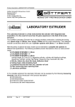
3.0 Experimental and Numerical Methods
Preface
This chapter provides additional information regarding the experimental and numerical
methods used for this research. The information contained within is meant to supplement the
brief descriptions provided in later chapters (manuscripts) and provide a guide for future
Polymer Processing Laboratory personnel.
3.0 Experimental and Numerical Methods
123
This chapter presents relevant details regarding the materials studied, the experimental
apparatus and procedure followed, and the numerical methods utilized to fulfill the research
objectives identified in the previous chapter. Section 3.1 identifies the polyethylene resins that
are used during the course of this work. Section 3.2 presents the rheometric test methods used to
characterize each of the polyethylene resins. Sections 3.3, 3.4, and 3.5 summarize the
experimental apparatus and methods used for the melt fracture analysis, flow visualization, and
pressure profiling, respectively. Lastly, section 3.6 will review the hardware and software used
for performing numerical simulations as well as the software execution procedure.
3.1 Materials Studied
This work focuses on the rheology and flow behavior of two classes of polyethylene
resins. The first class of resins is the crux of this research project and consists of sparsely longchain branched and linear metallocene-catalyzed polyethylenes (MCPE). These materials are
compared and contrasted in order to understand the subtle effects of sparse degrees of long-chain
branching on the flow behavior of narrow molecular weight distribution polyethylene resins.
The second class of materials includes the ``conventional" PE resins. Specifically, highly
branched LDPE and strictly linear LLDPE are included in this particular classification. These
resins serve as branched and linear controls with which to compare to the MCPE resins, and thus
gauge their processability.
3.0 Experimental and Numerical Methods
124
Table 3.1: Polyethylene Resin Data
Mw
Mw/Mn
Mz
LCB
/104 C
Exact 0201
Exact 3132
Affinity PL1840
Affinity PL1880
88 700
111 000
87 400
115 800
2.14
2.04
2.43
2.12
158 900
180 400
160 200
183 700
0.79
—
0.57
0.18
NTX101
NA952
122 700
235 500
3.44
17.1
319 700
2 619 300
—
39a
Resin
a
: C13 NMR measurement
3.1.1 Metallocene-Catalyzed Polyethylenes
The metallocene-catalyzed polyethylene resins are divided into two groups. The first
group consists of sparsely long-chain branched resins and the second consists of strictly linear
resins. The reasons for having both groups is to understand the overall significance of longchain branching on rheology and flow behavior, and to better quantify the sensitivity of flow
properties to branch content. All of the MCPE resins analyzed in this study are commercially
available resins developed for film blowing applications. Furthermore, none of these film-grade
resins contains processing aids or slip/antiblock agents that might alter their inherent melt flow
behavior.
All of the MCPE resins have been characterized by researchers at Dow Chemical
(Freeport, TX) using high-temperature gel permeation chromatography (GPC) coupled with
dilute solution low-angle laser light scattering (LALLS). The theoretical basis for this particular
technique can be found elsewhere [Zimm(1949)]. This combined-technique method provides
typical molecular weight distribution curves, but also gives an indication of the long-chain
branch content. The molecular characteristics of each of the MCPE resins are tabulated in Table
3.0 Experimental and Numerical Methods
125
3.1. All of the MCPE resins used in this study have narrow molecular weight distributions
(MWD ~ 2), characteristic of metallocene-catalyzed polyolefins.
The sparsely branched MCPE resins contain different degrees of long-chain branching
content. They include the Dow Affinity PL1840, Dow Affinity PL1880 and ExxonMobil Exact
0201 resins. The Dow Affinity resins have been produced using the Dow constrained-geometry
[metallocene] catalyst (CGC) technology spoken of in Section 2.1, while the Exact resin has
been produced using the EXXPOL® catalyst technology. Table 3.1 shows that the Affinity
PL1880 resins contains the lowest branch content of the three resins at 0.18 LCB/10000 carbons,
but has the highest weight-averaged molecular weight (Mw) at 115,800 g/mol. Conversely, the
Exact 0201 resin has the highest branch content at 0.79 LCB/104 carbons, yet one the lowest Mw.
The Affinity PL1840 is similar in molecular weight to the Exact 0201 resin, but has an
intermediate degree (0.57 LCB/104 carbons) of long-chain branching. All of the branched MCPE
resins described are ethylene-octene copolymers.
The linear MCPE resin used for this study is the Exact 3132 resin. Exact 3132 is
manufactured using the EXXPOL® catalyst technology. The linear MCPE resin has been
characterized in a similar manner to the branched MCPE resins and the results can be found in
Table 3.1. The molecular analysis confirms that no long-chain branches are present, as expected.
The molecular weight and MWD are similar in value to the branched Affinity PL1880 resin.
Finally, the Exact 3132 resin is an ethylene-hexene copolymer.
3.1.2 Conventional Polyethylenes
In addition to the MCPE resins, a set of conventional polyethylene resins has been
investigated. The conventional resins include a high-temperature, high-pressure autoclave
3.0 Experimental and Numerical Methods
126
produced low-density polyethylene (LDPE) manufactured by Equistar, and a Ziegler-Natta
polymerized ethylene-hexene copolymer produced by ExxonMobil. The conventional LDPE is
commercially designated as NA952 and has a melt flow index of 2.0; the conventional LLDPE is
commercially designated as NTX101 and has a melt flow index of 0.9. Furthermore, the
molecular characteristics of each of these resins can also be found in Table 3.1. Neither resin has
processing aids nor slip/antiblock agents that might obscure their true melt flow behavior.
Although these resins represent more complex fluids, with broader molecular weight
distributions than the MCPE resins, they embody the typical responses of branched and linear
polyethylenes, respectively. Therefore, these conventional resins will serve as experimental
controls with which to compare the branched and linear MCPE resins.
3.2 Rheological Characterization
In order to realize the effects arising from molecular structure, and more specifically from
long-chain branching, the rheological properties of these resins must first be measured.
Rheological characterization is generally divided into two separate flow kinematics: shear and
shear-free flows. The kinematic arguments and relevant equations are presented earlier (Section
2.2.1). In this section, the apparatus used to perform rheological measurements and the operating
procedures used to acquire kinematic specific data will be presented.
3.2.1 Shear Rheology
The shear rheological measurements can be further divided into two categories. These
two categories are homogeneous and nonhomogeneous shearing flows. Homogenous flows are
characterized by deforming stresses that are independent of position, while nonhomogeneous
3.0 Experimental and Numerical Methods
127
flows exhibit spatial dependence. This comparison is the same as that between drag flows and
pressure-driven flows. In this study, a torsional rheometer has been used to obtain homogeneous
rheological data and a capillary rheometer has been used to obtain nonhomogeneous rheological
data. Although both methods provide shear viscosity, the versatility and range of data available
differs.
Torsional Rheometry
Steady shear and small-amplitude dynamic oscillatory experiments are performed using a
Rheometrics Mechanical Spectrometer Model 800 (RMS-800). The RMS-800 is a controlled
strain torsional rheometer capable of steady angular rotation and dynamic oscillatory
displacements. A dual range force rebalance transducer (FRT) is used to measure both torque
and normal force response during testing. Each test is performed within an inert nitrogen
environment using cone-and-plate test fixtures having a plate diameter of 25mm and a cone
angle of 0.1 radians. This particular configuration provides the most accurate rheological data
due to the homogeneous deformation field.
The RMS-800 provides viscoelastic data in the range of 0.001 to 100 s-1. Steady shear
deformation provides shear viscosity (η) and primary normal stress difference (N1) data in the
range of 0.001 to 1.000 s-1. Small-strain dynamic oscillatory deformations provide complex
viscosity (η*), storage modulus (G'), and loss modulus (G'') data in the range of 0.1 to 100 rad/s.
In most cases, the Cox-Merz rule has been assumed to hold true (w = g).
3.0 Experimental and Numerical Methods
128
Capillary Rheometry
Nonhomogeneous steady shear experiments at shear rates greater than 10 s-1 are
performed using a Goettfert Rheograph 2001 (RG2001).
The RG2001 is a controlled
displacment capillary rheometer capable of volumetric displacements of 3.5 cm3/s and applied
loads of 20 kN. The dies used for rheological analysis are tungsten carbide steel capillaries with
die diameters of 1 mm and lengths of 10, 20, and 30 mm. Furthermore, each of the dies has a
180° included entry angle (flat entrance) and a barrel-to-capillary contraction ratio of 15.
The RG2001 provides steady shear viscosities (η) in the range of 10 to 1000 s-1. Because
of the nonhomogeneous flow field the steady state shear viscosity is the only relevant quantity.
The limits of accuracy are determined by the sensitivity of the mounted pressure transducer at
low rates and the onset of melt fracture at high rates. Due to the large contraction ratio, a Bagley
end analysis is typically performed to correct the effects of entrance pressure loss on the wall
shear stress and shear viscosity. Furthermore, the Rabinowitsch correction is also utilized to
correct for non-parabolic flow profiles within the capillary.
3.2.2 Extensional Rheology
Uniaxial extensional measurements are carried out using a Rheometrics Extensional
Rheometer Model 9000 (RER-9000). The RER-9000 is based on the original design by H.
Munstedt (1979) in which a homogeneous molded cylindrical sample is suspended in a heated oil
bath and fixed between a stationary platform and a mobile drawing arm. Figure 3.1 represents a
basic schematic of the device. The density of the oil (Dow Corning Fluid 200) is so chosen to
match the resin density at the test temperature, therefore creating a neutrally buoyant
environment. The applied force resulting from deformation is measured using a linear variable
3.0 Experimental and Numerical Methods
129
Optical Encoder
Stepper Motor
Thermal Jacket
Moveable Rod
Oil Bath
Sample
LVDT & Leaf Spring
Assembly
Figure 3.1: RER9000 Schematic
differential transformer (LVDT).
A viewing window is used to assure that homogeneous
deformation of the sample occurs.
The RER-9000 provides homogeneous uniaxial deformation at a specified applied strain
rate or stress. The instrument is capable of applying extensional strain rates from 0.001 to 5 s-1,
however the practical limit is generally found to be 1 s-1. The maximum strain, using 22 mm
samples, is typically found to be 3.0 strain units. Because the presence of a free surface often
leads to nonhomogeneous or nonuniform deformation, many duplicate tests are performed.
Those samples that ``appear" to deform uniformly are averaged to obtain a statistical response
for a given strain rate and strain.
3.3 Melt Fracture Analysis
The experiments examining the melt fracture behavior of metallocene and conventional
polyethylene resins were found to require two key components. The first component consists of
3.0 Experimental and Numerical Methods
130
a pumping device capable of accurately metering polymer melt at a desired flow rate. The second
component is an imaging device that can resolve both gross and fine features of extruded
samples.
In the following section, the chosen apparatus and operating procedures used to
perform the melt fracture studies will be outlined.
3.3.1 Apparatus
The Goettfert Rheograph 2001 (RG2001) capillary rheometer (see Section 3.2.1) was
chosen as the metering device for this study. The RG2001 is a positive displacement pump that
provides very accurate metering of polymer melt through round capillary dies. The RG2001 is
fitted with a pre-contraction pressure transducer port that is used to measure transient and steadystate driving pressures. Additionally, a high-speed data acquisition system consisting of a 12-bit
A/D acquisition card (Model ADM12-11) by Quatech and an IBM-compatible personal
computer (PC) are utilized to rapidly measure pressure fluctuations during slip-stick flow
conditions.
The imaging device chosen for this study is either a Cambridge Instruments Stereoscan
Model 200 scanning electron microscope (SEM) or a Leo 1550 field emission scanning electron
microscope (FE-SEM). An SEM was found to be most versatile because it can provide both
coarse and fine resolution micrographs of the extruded melt fracture samples. Furthermore,
scanning electron microscopy provides greater image contrast than optical microscopy when
imaging semi-transparent materials like polyethylene.
3.0 Experimental and Numerical Methods
131
3.3.2 Operating Procedure
In the next two subsections, detailed instructions for obtaining and imaging melt
fracture specimens using the apparatus described earlier are provided.
Sample Collection
1. Prepare the Rheograph 2001 for operation according to the instrument user manual. This
step includes setting the operating temperature, installing the capillary die, and installing
and calibrating the pressure transducer.
2. Enter the desired piston rate (0.0001 to 20 mm/s) and activate the servo-hydraulic system.
3. Allow the driving pressure to equilibrate. If unsteady flow conditions occur, attach the
high-speed data acquisition system to the chart recorder input leads and capture the
sinusoidal pressure response.
4. Obtain multiple samples of the extrudate and quench in water.
5. Document the extrusion temperature, capillary dimensions, and pressure reading for each
sample collected.
6. Repeat steps 2-5 for each subsequent piston rate.
7. Repeat steps 1-6 for each extrusion capillary used.
Imaging
1. Securely mount each sample onto a separate specimen stage using conductive tape.
2. Sputter coat the specimens with 10nm thick layer of gold.
3.0 Experimental and Numerical Methods
132
3. Prepare the Leo 1550 for operation according to the instrument user manual. This step
includes mounting the specimen stages, evacuating the imaging chamber, and positioning
each specimen stage for imaging.
4. Obtain micrographs at 20x & 50x magnification.
5. Label the micrograph(s) appropriately and document relevant imaging parameters.
6. Repeat steps 4-5 for each melt fracture specimen.
3.4 Flow Visualization
The flow visualization experiments are very complex studies that consist of a large
number of components and require precise measurement of experimental quantities. The current
section will provide an overview of the apparatus and operating procedure used to obtain
isochromatic fringe patterns and particle streak patterns.
3.4.1 Apparatus
The flow visualization studies rely upon three key component systems: the polymer
delivery system, the visualization die, and the optical imaging system. The following three
subsections will summarize the individual devices that make up the component systems.
Polymer Delivery System
The polymer delivery system has been designed to provide pulseless, precisely metered
molten polymer at near isothermal conditions. This is accomplished using a 25.4mm plasticating
laboratory extruder (Killion) and 1.752 cc/rev gear pump (Zenith, HPB-5556). The gear pump is
driven by a 1/4 horsepower AC motor (US Electric Motors) that operates between 11 and 113
3.0 Experimental and Numerical Methods
133
ED
P
T
EM
GB
GP
T
T
P
T
E
Figure 3.2: Polymer Delivery System. E – Extruder, GP – Gear Pump Assembly, EM – Electric Motor,
GB – Gearbox Reducer (optional), ED – Extrusion Die, T – Temperature Probe, P – Pressure Probe.
rpm. Lower flow rates are obtained by placing a gear-reducing unit (Reynolds Ltd.) between the
motor and gear pump. The gear reduction ratio is 21.4:1. High-pressure conduit connects the
extruder and gear pump assemblies while a high-pressure conduit fitted with a Kenics static
mixer connects the gear pump to downstream equipment. The static mixing element is used to
thermally and mechanically homogenize the polymer melt.
The primary operating variables are flow rate and melt temperature. The flow rate is
manually adjusted by first varying the gear pump drive speed and then adjusting the extruder
screw speed to maintain acceptable back pressure on the gear pump inlet. An optical tachometer
3.0 Experimental and Numerical Methods
134
Figure 3.3: Visualization die schematics [White (1987)].
is linked to the gear pump drive shaft to determine the volumetric flow rate.
The melt
temperature is controlled by 4 sets of heating elements. The first set is found in the extruder, the
second on the extruder-gear pump connecting conduit, the third on the gear pump assembly, and
the fourth on the static mixer assembly. All four regions are regulated around a desired set point
via PID controllers.
Visualization Die
The visualization die used for this study is a planar contraction die originally designed
and constructed by S. White [White (1987)]. The basic features and dimensions of the die are
found in Figure 3.3. The die is machined from 316 stainless steel and features insert slots that
can be used to vary the contraction geometry. This study employs the previously machined 8:1
planar contraction geometry inserts. The upstream slit dimensions are 25.4 x 20.3 x 114.3 mm
(WxHxL) and the downstream slit dimensions are 25.4 x 2.54 x 25.4 mm. The machining
3.0 Experimental and Numerical Methods
135
tolerance is 0.026mm. Heating of the die is accomplished using three, independently controlled
sets of strip resistance heaters (Industrial Heater Co.).
The most unique features of the visualization die are the optical windows.
Two
rectangular windows are positioned on opposite sides of the contraction region. The optical
windows are made from commercial grade quartz (Dell Optics) and have dimensions of 25.4 x
31.7 x 63.5 mm (WxHxL).
The thickness was specifically chosen to withstand the large
hydrostatic pressures present at high flow rates. The windows are secured using silicone gasket
material and steel retaining brackets.
Optical Imaging System
The optical system is used to illuminate the flow field. The specific attributes and
components are determined by the particular study.
For flow birefringence studies, the
generation of isochromatic fringe patterns requires a monochromatic light source, polarization
optics, and imaging device [Janeschitz-Kriegle (1983)]. The monochromatic light source chosen
for this study is an unpolarized 0.5 mW He-Ne laser (Spectra Physics). The characteristic
wavelength is 632.8 nm. Because the beam diameter is only 0.9mm, it is expanded using a 10x
objective lens (Tower) and 76.2 mm collimating lens (Oriel). The expanded beam is then passed
through a ``polarizer" with its optic axis rotated 45 degrees from the flow direction. The
polarized beam passes through the visualization die and proceeds through the ``analyzer". The
analyzer is a matched polarizing optic with its optic axis orthogonal to the ``polarizer". The
resulting beam is then focused using a 76.2 mm focusing lens (Oriel) and imaged using a digital
camera (Sony TRV900).
All optic components are mounted to an optic rail to maintain
alignment.
3.0 Experimental and Numerical Methods
136
L
OL
CL
P
FC
A
FL
DVC
Figure 3.4: Optial Rail Assembly. L – Laser, OL – Objective Lens, CL – Collimating Lens, P – Polarizer
(Plane or Circular), FC – Flow Cell, A – Analyzer (Plane or Circular), FL – Focusing Lens, DVC –
Digital Video Camera.
The “polarizer” and “analyzer” can be either plane or circular polarizers. Plane polarizers
simply polarize the incident beam along the optic axis. Plane polarization gives rise to dark field
patterns which represent whole order fringes (N=0,1,2,...). On the other hand, circular
polarization combines a plane polarizer with a quarter wave plate. This combination yields a
retarded wave and gives rise to light field patterns which represent half order fringes (N=1/2, 3/2,
5/2, …). The mathematical details pertaining to flow birefringence can be found in Appendix G.
The particle streak patterns are produced using a much simpler setup.
White light
illuminates the flow cell at a 45 degree angle and reflects off of solid particles dispersed in the
melt stream. These particles are generated by adding 0.5% by weight of powdered nickel or iron
to the extruder feed. Generally, a small amount of mineral oil is added to better disperse the
powdered metal and prevent settling in the extruder throat. A digital camcorder (Sony TRV900)
is used to record the streaming particles. The recorded flow patterns are then manipulated using
Adobe Photoshop 5.0 to obtain time-lapsed streak patterns.
3.4.2 Operating Procedure
In the next three subsections, detailed instructions for obtaining isochromatic fringe
patterns and particle streak patterns are provided. A procedure common to both experiments will
be provided first, followed by experiment specific instructions.
3.0 Experimental and Numerical Methods
137
System Initialization
1. Turn on extruder and temperature controllers.
2. Set temperature setpoints and allow one hour soak time.
3. Set the zero and gain (80\% scale) of all pressure transducer indicators.
4. Feed polymer pellets into the extruder hopper and initiate screw rotation at 10 rpm.
5. Once considerable backpressure is observed (~1000 psi), reduce screw speed and initiate
gear pump motor (setting 0).
6. Bring gear pump motor to desired speed and adjust extruder screw speed to maintain
1000 psi back pressure on extruder pressure transducer.
7. Allow 30 minute purge period to remove resident polymer melt.
Isochromatic Fringe Patterns
8. Install and align the optic components as illustrated in Figure 3.4. Assure that the
expanded, collimated beam is centered around the contraction entrance along the neutral
flow axis (z-axis).
9. Obtain dark field stress patterns by placing the plane polarizers along the optical rail.
Insure that the polarization axes are crossed.
10. Replace the plane polarizers with the circular polarizers and obtain the light field pattern.
Insure that the quarter wave plates are facing each other and that the polarization axes
remain crossed.
11. Repeat steps 8 and 9 for each flow rate.
12. Extract still images for each flow rate using digital video software (MiroVideo 200).
3.0 Experimental and Numerical Methods
138
Particle Streak Patterns
8. Add the powdered metal tracers to the feed polymer and allow sufficient time for
complete dispersal of tracer particles across the viewing region.
9. Align the digital video camera with the visualization die and orient the light source to get
maximum reflection and contrast of the embedded tracer particles.
10. Record the flow from 5 to 20 minutes, depending on the imposed flow rate.
11. Repeat step 9 for each flow rate.
12. Extract the full motion video for each flow rate and generate streak patterns using image
manipulation software.
3.5 Pressure Profiling
The pressure profiling studies investigate the effects of an abrupt planar contraction on
the flow behavior of polyethylene melts. Specifically, the observed pressure drop along the flow
axis will be measured. The following section will summarize the key components of the
apparatus used, and the operating procedure used to perform the studies.
3.5.1 Apparatus
The pressure profiling apparatus is similar to that of the flow visualization studies. The
same polymer distribution system described previously is also used for metering polymer melt to
pressure profiling die. The main difference is that of the extrusion die utilized. The profiling die
was fabricated specifically for this study. The relevant dimensional schematics can be found in
Figures 3.5 and 3.6. The profiling die is machined from 440C stainless steel and consists of six
pressure transducer ports machined along the slit flow path. Four of these ports are placed
3.0 Experimental and Numerical Methods
139
Figure 3.5: Profiling Die (Top half)
3.0 Experimental and Numerical Methods
142
Figure 3.6: Profiling Die (Bottom Half)
3.0 Experimental and Numerical Methods
143
upstream of the abrupt 4:1 planar contraction, the remaining two ports are found downstream.
The upstream slit dimensions are 12.7 x 2.54 x 108.0 mm (WxHxL) and the downstream
dimensions are 12.7 x 0.635 x 25.4 mm (WxHxL). These dimensions were chosen in order to
augment the maximum achievable shear rate to approximately 100 s-1.
The pressure measurements were obtained using melt pressure transducers (Dynisco
PT422A) with maximum pressure ranges from 34.5 to 103.4 bars (500 to 1500 psi). Calibration
of these transducers was performed using a dead weight tester (Model No. 23-1) manufactured
by Chandler Engineering (Tulsa, OK). Practical pressure measurements were obtained using
scaled pressure indicators (Dynisco ER478) or the Quatech A/D data acquisition card described
earlier.
Temperature control of the die is accomplished using two enclosing aluminum heating
plates that are securely fastened to the top and bottom faces of the die. The aluminum plates
have been pre-drilled to accept twelve 150W 6.35 x 38.1 mm (0.25 x 1.5 in.) cartridge heaters.
Combined with appropriate temperature controllers (Omega CN9000), these heating plates
provide near isothermal flow conditions within the profiling die.
3.5.2 Operating Procedure
The current subsection provides instructions for initializing the polymer delivery system,
preparing the profiling die for use, and obtaining pressure measurements during operation.
System Initialization
1. Turn on extruder and temperature controllers.
2. Set temperature setpoints and allow one hour soak time.
3.0 Experimental and Numerical Methods
144
3. Set the zero and gain (80\% scale) of all pressure transducer indicators.
4. Feed polymer pellets into the extruder hopper and initiate screw rotation at 10 rpm.
5. Once considerable backpressure is observed (~1000 psi), reduce screw speed and initiate
gear pump motor (setting 0).
6. Bring gear pump motor to desired speed and adjust extruder screw speed to maintain
1000 psi back pressure on extruder pressure transducer.
7. Allow 30 minute purge period to remove resident polymer melt.
Pressure Measurements
8. While the polymer distribution system components are heating: attach the heating plates,
install the pressure transducers, and initiate heating of the profiling die. Allow a onehour soak and then set the zero and gain (80% scale) for all pressure transducer
indicators.
9. During operation, record the indicated pressure for each of the six melt transducers.
10. Repeat step 9 for each subsequent flow rate.
3.6 Numerical Simulations
Numerical simulations are performed to assess the ability to predict the flow behavior of
the metallocene and conventional polyethylene resins under complex flow conditions. The
computational method and capacity greatly determine the practical limits of computational
efficiency. In the following subsections, the hardware and software packages used to perform
numerical simulations, and the numerical procedure used to obtain flow predictions are
summarized.
3.0 Experimental and Numerical Methods
145
3.6.1 Hardware & Software
All of the numerical simulations undertaken in this project were performed using a
Silicon Graphics Inc. (SGI) Origin 200 server. The Origin 200 is a deskside, entry level
workgroup server supporting one to four MIPS processors. Currently, the Origin 200 is fitted
with two 270 MHz IP27 RISC processors and 512 MB of main memory. The installed 64-bit
operating system is IRIX 6.5.10f. In addition to the numerical simulations, the curve and
parameter fitting calculations are performed using a personal Pentium III 733 MHz computer.
The software used for this study can be divided between two classifications, parameter
fitting applications and finite element method simulations. The parameter fitting software is selfwritten and coded in the Fortran 90 conventions. Absoft Pro Fortran 6.0 (academic) is used to
compile the source code into an executable format.
Fitting programs for the Generalized
Newtonian Fluid (GNF), Phan-Thien and Tanner (PTT) and McLeish-Larson Pom-Pom models
have been written. Furthermore, IMSL numerical subroutines, available from Visual Numerics,
are used to solve ordinary and partial differential equations as well as numerical integration
calculations. A complete listing of all relevant Fortran 90 source code is found in Appendix D.
The finite element method simulation software used for this study is Polyflow 3.8
(Fluent). This particular version is written for the IRIX operating system and therefore used on
the SGI Origin 200 server.
The Polyflow 3.8 software suite consists of four discrete
applications: GAMBIT, Polydata, Polyflow, and FlPost. The GAMBIT application is used to
define and mesh the desired flow region. Polydata is used to specify simulation parameters: the
flow boundary conditions, the chosen constitutive equation, the interpolation techniques, and
local and global convergence criteria. Polyflow is the finite element method solver and actually
3.0 Experimental and Numerical Methods
146
performs the simulation calculations. The final application, FlPost, is a postprocessor application
and provides visualization of the simulation results in a convenient, graphical manner.
3.6.2 Procedure
The procedure used for obtaining accurate numerical simulations does not follow a strict
“operating procedure”, but rather a methodology. In this section, a method for performing
numerical simulations that are derived from physical experiments and calculated from available
rheological data is outlined. Although this approach may not be deemed the most accurate or the
most efficient, it has been determined to be the most consistent one across many different fluid
descriptions.
Parameter Fitting
Parameter fitting is arguably the most important step involved in obtaining accurate
numerical predictions. It is during this step that experimentally measured data is translated into a
considerably smaller set of constitutive parameters. Therefore, it is very important to understand
the flow kinematics and range of applicability associated with the rheological measurements in
comparison to that of the simulated geometry. Excessive extrapolation of rheological properties
beyond experimentally measured bounds may lead to significant inaccuracies in the resulting
numerical predictions.
The parameter fitting method consists of three steps. The first step is fitting available
linear viscoelastic data to obtain the discrete relaxation spectrum. Linear viscoelastic data is
usually comprised of G’, G’’, and η in the zero-shear viscosity plateau. The discrete relaxation
spectrum, composed of a finite number of relaxation times and strengths, is calculated using the
3.0 Experimental and Numerical Methods
147
fitting programs. The general rule of thumb is one relaxation time per decade of data. The fitting
algorithms implement non-linear least squares minimization to obtain the relaxation strengths at
each user-supplied relaxation time.
The second step involves the fitting of the nonlinear shear parameters found within each
of the constitutive equations investigated. Because all of the parameters in the GNF model are
nonlinear shear parameters, nonlinear regression is used to obtain the model parameters by
reducing the sum of the squared errors. For the PTT model, the ξ parameter is the nonlinear
shear parameter, while for the Pom-Pom model τs is the respective nonlinear parameter. The
difference between each of these parameters is the source of rheological data used for fitting. ξ
is generally determined from manual shifting of η(g) to overlay on η’(ω) data. Therefore
numerical fitting is not utilized. τs is significantly more difficult to obtain from shear data alone
and is often determined with the use of extensional data as well. The combination of the
nonlinear shear parameter and discrete relaxation spectrum provides more accurate predictions
during pure shear deformations.
The final step is fitting extensional viscosity growth data to obtain the shear-free
parameter. For the PTT model, ε is the nonlinear shear-free parameter, while for the Pom-pom
model, q is the nonlinear shear-free parameter. In addition to the relevant rheological data, the
use of the discrete relaxation parameter and non-linear shear parameters is also required.
Because of the strain-hardening nature of branched PE resins, it is very difficult to obtain steady
extensional viscosities. Therefore, most of the available data is transient extensional viscosity
data.
3.0 Experimental and Numerical Methods
148
Polyflow Simulations
The Polyflow numerical simulations follow are very straightforward method for
performing finite element method calculations on user-defined flow domains. As mentioned in
the ``Hardware \& Software" section, there are four discrete applications used to setup, execute,
and analyze the numerical simulations.
Figure 3.7 illustrates the process for carrying out
numerical simulations using the Polyflow software suite. A comprehensive description of each
application can be found in the respective Polyflow manuals [Polyflow (1998)].
The first application is the GAMBIT mesh generation package. This software application
generates two- or three-dimensional, structured or unstructured, finite element meshes.
Furthermore, triangular or quadrilateral element geometries are available for 2-D meshes. The
user-supplied information includes the mesh dimensions and boundary types. The resulting
mesh file is known as a GAMBIT neutral (NEU) file. This mesh file is utilized by the Polydata
software application.
The next user-activated application is Polydata. Polydata is used to specify simulation
parameters, including: boundary conditions, constitutive equations, variable interpolation
techniques, and convergence criteria. Polydata uses the NEU mesh file described above and
converts it to a Polyflow compatible MSH file. Polydata then uses this mesh file to map
appropriate boundary conditions. The simulation data file (DAT) produced by Polydata is then
used as primary input for the finite element solver, Polyflow.
Polyflow is the actual FEM solver. This software application uses the Polydata DAT file
as input and generates various output files. The primary outputs are the Fluent mesh (FLUM)
and Fluent result (FLUR) files. These files contain the nodal solutions for each independent
variable (pressure, velocity, and stress). Furthermore, the Fluent output files are also output for
3.0 Experimental and Numerical Methods
149
each evolutive step of the simulation. This is very useful for analyzing the flow development as
a function of flowrate or viscoelastic character. Optionally, result probe files (PRB) can be used
to monitor variable values at specific locations or nodes within the flow geometry.
The final application is the simulation postprocessor, FlPost. FlPost uses the Fluent
output files from Polyflow to visualize the results. Flpost provides pressure, velocity, stress, and
streamline contours across the flow domain. These contour patterns can be saved in a graphic
format (EPS, TIFF) or printed for future use. Additionally, nodal values can be plotted and/or
saved to disk for later use as well.
3.0 Experimental and Numerical Methods
150
Figure 3.7: Polyflow Simulation Procedure
3.0 Experimental and Numerical Methods
151
3.7 References
Janeschitz-Kriegl, H., Polymer Melt Rheology and Flow Birefringence, Springer-Verlag, New
York, 1983.
Münstedt, H., J. Rheol., 23, 421 (1979).
Polyflow S.A., Belgium, Polyflow 3.8, 2000.
White, S.A., The Planar Entry Flow Behavior of Polymer Melts: Experimental and Numerical
Analysis, Ph.D. Dissertation, Virginia Tech, Blacksburg, VA, 1987.
Zimm, B.H. and H.W. Stockmayer, J. Am. Chem. Soc., 17, 1301 (1949).
3.0 Experimental and Numerical Methods
152