Download 1. How to read this manual

Preliminary version
RAMSETE
Acoustic forecast software
User manual
Version 1.0
1.1.94
GENESIS
Software and acoustic consulting
This manual has been written by Paolo Galaverna with the collaboration of Marzia Giabbani and the
supervision of Angelo Farina and transalted by Guido Truffelli.
Updated Wednesday, May 31, 1995.
Windows and Excel are trade marks registered by MICROSOFT CORPORATION
Surfer is a trade mark registered by G OLDEN SOFTWARE
AutoCAD is a trade mark registered by AUTODESK I N C.
Modeler is a trade mark registered by B OSE CORPORATION
Paint Shop is a trade mark registered by JASC IN C.
THIS SOFTWARE IS PROTECTED BY INTERNATIONAL COPYRIGHT LAWS. THIS MANUAL CAN'T
BE REPRODUCED BY NO MEANS WITHOUT THE AUTHOR'S WRITTEN PERMISSION
Summary
Summary ...................................................................................................................................................................................................................................III
1. How to read this manual ........................................................................................................................................................................................................5
1.1. Legend..............................................................................................................................................................................................................5
2. Introducing Ramsete..............................................................................................................................................................................................................6
2.1. Features ...........................................................................................................................................................................................................7
2.2. Computation Method.......................................................................................................................................................................................8
2.3. Versatility...................................................................................................................................................................................................... 12
2.4. Required Hardware ....................................................................................................................................................................................... 12
3. Ramsete applications ......................................................................................................................................................................................................... 13
3.1. Ramsete CAD................................................................................................................................................................................................ 14
3.2. Material Manager.......................................................................................................................................................................................... 15
3.3. Source Manager............................................................................................................................................................................................ 16
3.4. Ramsete Trace ............................................................................................................................................................................................. 17
3.5. Ramsete Graph............................................................................................................................................................................................. 18
3.6. Ramsete View............................................................................................................................................................................................... 20
3.7. Preferences .................................................................................................................................................................................................. 22
3.8. Paint Shop Pro ............................................................................................................................................................................................. 22
4. Using Ramsete .................................................................................................................................................................................................................... 25
5. Ramsete CAD....................................................................................................................................................................................................................... 34
5.1. File menu....................................................................................................................................................................................................... 35
5.2. Edit menu...................................................................................................................................................................................................... 37
5.3. Tools menu ................................................................................................................................................................................................... 38
5.4. View menu..................................................................................................................................................................................................... 44
6. Material Manager................................................................................................................................................................................................................. 48
7. Source Manager................................................................................................................................................................................................................... 51
7.1. File Menu....................................................................................................................................................................................................... 52
7.2. Edit Menu ...................................................................................................................................................................................................... 59
7.3. View Menu..................................................................................................................................................................................................... 59
7.4. Window Menu.................................................................................................................................................................................................62
7.5. Help Menu .....................................................................................................................................................................................................64
8. Ramsete Trace.....................................................................................................................................................................................................................65
9. Ramsete Graph....................................................................................................................................................................................................................69
9.1. File Menu .......................................................................................................................................................................................................71
9.2. Edit Menu.......................................................................................................................................................................................................73
9.3. Chart Menu ....................................................................................................................................................................................................73
9.4. Table Menu....................................................................................................................................................................................................75
9.5. Window Menu.................................................................................................................................................................................................77
10. Ramsete View....................................................................................................................................................................................................................78
10.1. File Menu.....................................................................................................................................................................................................79
10.2. Edit Menu ....................................................................................................................................................................................................82
10.3. View Menu...................................................................................................................................................................................................82
10.4. Map Menu....................................................................................................................................................................................................85
10.5. Blanking Menu ............................................................................................................................................................................................91
10.6. Surfer Menu.................................................................................................................................................................................................93
10.7. Help Menu...................................................................................................................................................................................................93
11. Render................................................................................................................................................................................................................................94
11.1. File Menu.....................................................................................................................................................................................................95
11.2. View Menu...................................................................................................................................................................................................95
11.3. Rendering Menu ..........................................................................................................................................................................................97
11.4. Output Menu...............................................................................................................................................................................................99
11.5. Help Menu...................................................................................................................................................................................................99
12. Troubleshooting...............................................................................................................................................................................................................101
12.1. Ramsete Trace .........................................................................................................................................................................................101
12.2. Ramsete Graph.........................................................................................................................................................................................101
12.3. Ramsete View...........................................................................................................................................................................................101
1.
How to read this manual
This manual has been written also for people that are not skillful computer users. For this reason we
apologize to more skilled users for the frequent repetitions of the most simple Windows usage
techniques.
I NTRODUCING RAMSETE shows the organization of the package and the basic algorithms used by its
components: Ramsete can be used nearly by everyone, but you can't become a do-it-yourself
acoustic engineer. If you really desire to exploit every feature of the program you need a deep
knowledge of its inner physical-mathematic heart.
K NOWING RAMSETE briefly shows step by step, the nine modules of the the package. By this way the user
can have a global view of the entire system.
USING RAMSETE is a practical example of a complete working session.
RAMSETE COMMANDS is the exhaustive list of all commands of every program of the package. This section
can be in its completeness or one paragraph at time as you need it.
RAMSETE MATERIALS includes all the standard materials contained in Material Manager by default, their
description and acoustic properties.
RAMSETE SOURCES contains all Source Manager's standard noise/music sources.
RAMSETE TROUBLESHOOTING describes known bugs or obscure error conditions that could rise by using the
program.
1.1.
Legend
F ILE MENU
Select a menu item: you can activate it by clicking on it with the left mouse button, otherwise you can
press the "Alt" key followed by "F" (without releasing it).
New
Select a menu command: you can select a command from a menu clicking on the desired item or by
pressing the underlined letter of its name (usually the first one). You can also use the arrow keys to
move onto a command and press Enter to select it.
Cut (Shift+Del)
Using a short-cut: if you can see a key combination on the right of a menu command you can recall it
simply by pressing the displayed keys, there's no need to open the corresponding menu.
$
%
See also...
Warning!
5
2.
Introducing Ramsete
6
Ramsete is an advanced software package for the acoustic phenomena simulation. Thanks to its
powerful features it can be used to study concert halls, auditoriums and theaters, or industrial
acoustic treatments and external noise sources.
It is a modular system that can be easily updated and used even by non professionals.
2.1.
Features
This program has been developed for the Windows operating system: so we've obtained an advanced
user interface, a fast learning curve, a full integration with the most popular PC working environment.
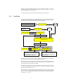
The system is composed by many modules connected in the following way:
Power Measures (ISO 3744)
Source Manager
data base
Lw,Q θ
Directivity Measures (speakers)
Material Proof
certificates
Material Manager
data base
R,α
AutoCad (TM)
Ramsete CAD
Geometry File (.RAY)
Pyramid Tracing
Impulse Responses File (.__*)
Post Processors
Surfer (TM)
Ramsete View
Perspective views,
Rendering, 2D and 3D mapping
Sound levels and other indexes
(isochromatic or contours)
Ramsete Graph
Impulse responses, decay curves
Ottave spectra, reverberation times
Sum of the impulse responses of
many sources
The system includes a simple 3D CAD, Ramsete CAD, that features axonometric and orthogonal
views of the room and can import/export DXF files generated by AutoCAD.
Material Manager and Source Manager have a good internal data base that can be edited by the end
user, who can let enter new materials and sources with all their acoustic parameters that can be
experimentally measured or automatically computed.
At the heart of the package there is Ramsete Trace, that receives a Ramsete CAD model as input and
computes the impulse responses for further processing. This program is based on a pyramid
tracing algorithm and geometric acoustics.
Ramsete Graph can post-process these impulse responses and give a graphic or tabular view of the
data. For each one of the ten frequency bands and for each receiver it can display the impulse
response, linear and A weighted; the SPL levels; the Schroeder decay curve and the reverberation
times: EDT, T 10, T 15, T 20, etc..
7
Ramsete View can display perspective views of the geometric models and it can render and map the
following data in two or three dimensions:
•
•
•
•
•
•
•
•
•
•
•
•
•
•
SPL
Ldir
Lrev
R/D
Lp-Lw
C50
C80
Tbar
Aeq
STI
RASTI
LE
Aeq2
ITDGeq
Sound Pressure Level
Direct Wave level
Reverberated field level
Klarheitsmass
Klarheitsmass
Barycentric Time
Equivalent Reflection Amplitude
Speech Transmission Index
Dresda group
Dresda group
Cremer, Kürer
Ando
Houtgast & C
Lateral Efficiency
Jordan
Initial Time Delay Gap
Beranek
In the last release has been added the possibility of anechoic music convolution with the impulse
response.
The customer may ask for personalized program versions in order to solve specific problems.
2.2.
Computation Method
We chose pyramid tracing because it guarantees the following benefits:
•
short computation times;
•
high resolution of the impulse response;
•
precise receivers positioning (modeled as points, not spheres).
The beam tracing, i.e. the modelling of the spherical sound waves through beams of various shapes,
is a natural evolution ray tracing. The simplest way to obtain a beam tracing is to implement a
normal ray tracing with spherical receivers, whose radius grows as the square of the ray length. In
this way we can keep constant the quotient between the sphere's maximum circle an the global
surface hit by the rays, reducing the minimum number or rays to compute. But there is a big
drawback with this approach, the receiver keeps getting bigger and bigger, growing well past the
room dimensions, thus it could receive energy even from rays on the other side of a wall or outside
the room.
A much better way to achieve the same effect is to trace diverging rays or cones and to use pointshaped receivers. When a receiver is contained into a cone it receives a energy intensity computed
with the following formula:
 Qϑ ⋅ ∏ (1 − αi ) 
i

L p = LW + 10 ⋅ log
4
⋅
π
⋅r2


(1)
that's equivalent to the image sources formula. With this approach we have another problem: we can
cover the entire sphere surface with circles without overlapping them at least partially. Pure cone
tracing has been improved with a statistical method in which the energy decreases like a Gaussian
curve with the distance from the cone axis. This is the algorithm adopted in Epidaure, a program
written by Vian, Martin and Maercke.
Naylor, in the Odeon package, uses a cone tracing preprocessor for a image source method. He
removes duplicate sources by using the reflection tree of the overlapping cones. This program can
achieve better results than the former one, adopting a nearly deterministic method.
Lewers is the first to successfully implement pyramid tracing, so that radically solves the beam
overlapping problem but loses the contributes of high order image sources. He tried to solve this
shortcoming superimposing a diffusive model to the deterministic pyramid tracing.
8
The biggest drawback of beam tracing is the incapacity to compute the reverberation queue
precisely, in fact, as the cones grow larger, a bigger number of image sources has been lost. Let's
try to explain it with the following example:
Pyramid axis
(cone or beam)
Receiver n. 1
Reflecting surface
Sound source
Receiver n. 2
Pyramid axis
(cone or beam)
In this way we need to correct the computed impulse response through an additive or multiplicative
method, but neither one can be safely applied in these conditions, where statistical acoustics
hypothesis are not met.
Ramsete has been developed with the explicit intention of solving all the limits of these kind of
modelling that fits well in wide environments such as theaters and factories.
Our pyramid tracer keeps in account the diffraction caused by free edges of shielding wall or other
hurdles, and computes the energy that passes through surfaces with a finite phono-insulating
property.
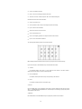
Next picture shows the isotropic sphere subdivision according to an algorithm studied by
Tanenbaum et al, based on the progressive bisection of the spherical surface starting from eight
triangles:
9
The tracer follows a pyramid’s history to a fixed depth or on a time basis, in order to build the full
sound queue of each receiver. It doesn’t make any assumption on the acoustic field diffusion, so that
we can have different reverberation times for each point, double slope decays, highly delayed echoes,
etc.
The necessary sound queue correction is of multiplicative type. It’s based on the assumption that
the number of impact on a receiver in the time unit n(t), can be mathematically described by the
following relation, according to Maercke/Martin:
4 ⋅ π ⋅ c03 ⋅ t 2
n( t ) =
V
l

−
4⋅c
⋅ 1 − e

cm
2
⋅N
2
0 ⋅β
⋅ t2
t
 4 ⋅ π ⋅ c3 ⋅ t 2 
− 
0
 =
⋅ 1 − e t 
V



2
c
2
(2)
The theoretical behavior of this curve is represented by the first factor of the above relation, ignoring
the bracketed term, thus it grows with the square of the time.
As far as the variable “t” reaches infinity, the relation (2) gives the number of impact into the time
unit:
n( ∞ ) =
N ⋅ c0 ⋅ lcm 2 π
⋅
V
4⋅β
(3)
In the two formulas above there are two parameters that depend on the acoustic field nature: the
minimum free path or lcm , that Ramsete computes following the axis of each pyramid, and the
adimensional coefficient
β,
that depends on the sabinian properties of the acoustic field (in a
perfectly diffused field we have β=0.3).
The critical time that appears in the relation (2), represents the ideal separation point between the
first half of the acoustic queue, in which all image sources are correctly found, and the second half in
which we have a constant energy addition per time unit. The following picture shows the comparison
between real situation and theoretical assumptions:
Reflections / ms
Theoretical curve
Critical time
Real curve
Mean value
computed by
Ramsete
Maercke-Martin theory
Time (ms)
The correction of the reverberating queue is computed by dividing the sound energy by the bracketed
term of equation (2), that’s always less than 1 and decreases with time t linearly.
In practice the estimate of the tc parameter is tied to α proper value of the b coefficient that
minimizes the difference between the exact curve and the estimated one. When we have found a
good value for β we can safely trace as few as 256 pyramids without any significant precision loss.
10
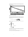
The following graph compares the energetic impulse responses obtained with an high number of
pyramids (128,000) and a small number (256) of them with two different queue correction
coefficients (β=0.3 and β=0):
We can see that in a non-sabinian room, the queue correction can obtain very good results with a
small computational effort (a couple of minutes).
In Ramsete we have the possibility of declaring some surfaces as “obstructing” in order to give the
system the chance to compute the energy faction that passes through some faces and hits receivers
on the other side, or diffracts along their free edges. This energy is computed with the
Keller/Maekawa formula:

2⋅π ⋅ N 
Ldiff = Ldir − 5 − 10 ⋅ log

 tanh 2 ⋅ π ⋅ N 
(4)
where Ldir is the direct level, assuming no obstructing face between the source and the receiver, and
N is the Fresnel number i.e.:
A
B
d
R
S
δ =A+B-d
N=
2
2⋅ f
⋅δ =
⋅δ
λ
c0
Thanks to these features, Ramsete can study the acoustic propagation in geometrically complex
rooms, with partial or total shields. It allows also the computation of the noise emission towards
receivers outside the room containing the source.
We can use this system in external environments where the distance between a fixed source and the
receivers is not very long, so that we can ignore atmospheric conditions.
11
2.3.
Versatility
Versatility is one of the key points of the package: it can be used inside industries, were the sound
pressure level is the main variable. SPL can be computed in 10 octave bands (31.5 - 16,000 Hz),
keeping into account the room geometry, the materials and their acoustic properties.
The noise generated by the machines can be simulated by sources freely placed, of which we know
the emitted power spectrum. We can introduce shields or barriers in order to simulate the noise
source encapsulation assigning a particular emission spectrum.
Each source emission is computed separately, so that we can value the incidence of each one on the
total level, suggesting the source that needs a particular care in shielding process.
Inside an auditorium or a concert hall the most important variable elements (other than the impulse
response) have been listed by many research groups in the last years and Ramsete can compute
nearly all of them.
We can introduce omnidirectional and isofrequencial sources, or real loudspeakers with a precise
frequency response and spatial dispersion.
2.4.
Required Hardware
The minimal required hardware is a 80386 processor, better if coupled with a 80387 math
coprocessor. Ramsete is an intensive CPU user and it works better on faster machines ('486 or
Pentium) but has not excessive RAM requirements: 4 Mb will suffice, but we all know that Windows
can be used productively starting from 8 Mb. You need at least a 20Mb of hard disk space in order to
set up Ramsete and run a simple working session. A good sound card is optional.
12
3.
Ramsete applications
13
The Ramsete package is composed by the following programs:
3.1.
•
Ramsete CAD
•
Material Manager
•
Source Manager
•
Ramsete Trace
•
Ramsete Graph
•
Ramsete View
•
Preferences
•
Paint shop pro
Ramsete CAD
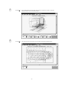
This program is a real 3D CAD system that can import DXF files generated by AutoCAD. You can
work on many views at the same time: plant, sections and axonometry. This is an example of a
typical Ramsete CAD screen:
14
There’s a floating toolbar that allows the selection of all the main geometric entities: floor, wall, roof,
door, window. The current cursor position is always displayed in the bottom line of the tools window.
You can insert sources and receivers, all with their orientation. This is very important for directive
sources and for Lateral Efficiency computation. Geometric model are saved in a human readable
.RAY format or in .DXF format readable by AutoCAD.
3.2.
Material Manager
This program has a spreadsheet-like interface where you can enter the acoustic properties of your
materials. You can display and edit the following parameters for each frequency band: absorbing
coefficient α, phonoinsulating power in dB R.
15
3.3.
Source Manager
This application can generate or display .SPK files, that contain all sound source data. With the ISO
3744 (3746) module you can input directly the sound level of a sound/noise source experimentally
measured:
You can use conform surfaces with 8 microphones, parallelepipedal surfaces with 5 or 9
microphones or hemispherical surfaces with 10 microphones.
All these parameters can be edited in tabular form and displayed in graphical form.
Source Manager can import .MDL files generated by Modeler (Bose Corporation).
16
3.4.
Ramsete Trace
This program is the pyramid tracer, the computation engine of the system:
17
3.5.
Ramsete Graph
This program displays in tabular or graphical form the results of the pyramid tracer, such as impulse
response in each receiver point or mean of the room:
integrated response (Schroeder decay curve):
18
octave spectrum in every receiver point:
numerical tables (SPL, reverberation times):
These tables can be easily exported to any spreadsheet application (Excel or Quattro-pro) by
performing a simple “copy and paste” clipboard operation.
19
3.6.
Ramsete View
The program postprocesses CAD models and Ramsete Graph data and generate perspective views of
the rooms mapping all the acoustic data in three dimensions. You can display the room from every
point of view by simple positioning of an imaginary camera:
You can map the computed parameters in two dimensions:
or three dimensions:
20
You can map isolevel curves in two or three dimensions:
21
You can choose between many rendering effects, so you can create professional looking presentation
without any complex dedicated software:
3.7.
Preferences
Using the notepad Windows applet you can edit the default parameters of Ramsete.
3.8.
Paint Shop Pro
This a very powerful shareware program that let you capture, edit and print any kind of image with
the desired color depth:
22
23
4.
Using Ramsete
25
Now we'll try to learn the basics of Ramsete following all steps of a typical application.
We want to map the situation created by a concentrated noise source in a reverberating environment,
i.e. a factory. We measured on site the reverberation time and the sound pressure level of the noise
source according to ISO 3744 (3746) standard. We also annotated the size and the materials the
factory was made of.
•
We'll start inserting into Source Manager all the data measured with the phonometer in order to
create a noise source with the same characteristics of the real one.
•
Then we'll sketch the factory geometry using Ramsete CAD, assigning the proper material to
each face. Finally we'll properly place the noise source and the receivers.
•
We'll use Ramsete Trace to create a file with all the results.
•
Finally we'll use Ramsete Graph and Ramsete View to analyze these results, verifying the
similarity between the computed reverberation time and the one measured on site. We'll have to
modify the geometric model and the source parameters until the two reverberation times are
equal.
•
Now we'll be able to study an intervention to improve the acoustic situation. We'll edit our model
with Ramsete CAD and recalculate the result file in order to verify the benefits or the drawbacks
of our improvements.
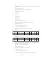
Below we are presenting the data measured following the ISO 3744 (3746) standard with a
parallelepipedal envelope surface with five measure points. The machinery dimensions are:
width: 2 m
length: 2 m
height: 4 m
The pressure level and the reverberation time T 60 (temperature = 20, humidity = 65%) are:
Frequency:
31.5Hz 63Hz
125Hz 250Hz 500Hz
1khz
2khz
4khz
8khz
16KHz
Lp(1)
92.50 91.00 96.40 97.30 95.20 92.50 94.60 90.40 90.20 90.50
Lp(2)
98.90 99.70 94.50 96.60 97.40 92.40 91.50 93.50 93.50 92.90
Lp(3)
85.80 88.30 85.60 82.40 85.40 86.40 85.80 82.30 84.30 85.20
Lp(4)
77.30 76.90 73.40 79.40 76.80 75.60 76.40 74.40 72.30 71.30
Lp(5)
66.30 68.90 63.90 70.40 72.10 65.40 62.60 64.60 66.40 61.90
RevTime:
31.5Hz 63Hz
T
12.2
12.0
125Hz 250Hz 500Hz
10.6
8.5
The factory volume is 2112 m3.
26
7.4
1khz
2khz
4khz
8khz
16KHz
7.0
7.0
5.2
2.2
0.6
The floor is made of concrete, the walls and the roof are made of rough-cast, the main door is made
of iron.
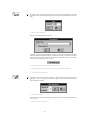
Now we can create our noise source following these steps:
•
click on Source Manager's icon
•
click on File menu item
•
click on the Crate Source ISO 3744... item
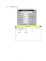
Now a dialog box will pop up to let us doing the following operations:
•
Select the number of microphones (5) from the corresponding list box;
•
Input length (2 m), width (2 m) and height (4 m) in the proper edit boxes;
•
Input the factory volume in the corresponding edit box (2112 m3);
•
Fill the first five lines of the spreadsheet with the sound pressure of each frequency band;
•
Fill the last line with the reverberation times of each band.
Now the dialog box should look like this:
27
•
click on the "OK - proceed" button to accept all the inserted values;
•
the dialog box will disappear, now we should save our source data;
•
click on the "FILE " menu item;
•
click on the Save As... item;
•
save the file as "proof.spk" in the "machines" directory;
•
click on the "FILE " menu item;
•
click on the "Exit" item to quit the program.
Now we can use Ramsete CAD to draw the factory's geometry remembering the following simple
rules:
•
Don't exceed in drawing particulars that are mostly irrelevant from the acoustic point of view but
that can increase dramatically the computation times;
•
Use as few surfaces as possible;
•
Don't place a receiver at less than 1 m far from the nearest source;
•
Don't place a receiver at less than 10 cm from the nearest surface;
•
Check if all the edges are well closed (matching) to avoid undesired pyramid escapes.
Let's start drawing the floor:
•
Execute Ramsete CAD by clicking on its icon from the Program Manager;
•
Click on "LENS" icon and adjust the window scaling right-clicking with the mouse until you can see
an area of 24 x 16 m;
28
•
Click on "Floor" icon;
•
Place the mouse cursor at position 0.00, 16.00, 0.00 and keep the left button pressed until you
reach position 24.00, 0.00, 0.00;
•
Input a "0" elevation for the floor in the dialog box and press the "OK" button;
•
Select the "Concrete floor (g)" from the material dialog box and press the "OK" button;
Now we are going to draw the walls:
•
Click on "Wall" Icon;
•
Click on the origin (0,0,0);
•
Drag the pointer to 0.00, 16.00, 0.00 and release the mouse button;
•
Input "0" and "6" in the elevation dialog box and press "OK";
•
Choose "Rough-cast" from the materials dialog box and press "OK";
•
Repeat the preceding steps for the other walls following these coordinates:
0.00,16.00,0.00; 16.00,24.00,0.00; 24.00,16.00,0.00; 24.00,0.00,0.00; 0.00,0.00,0.00.
Now we are going to draw the roof:
•
Click on "Roof" icon;
•
Click on position 0.00, 16.00, 0.00 and drag the pointer to 2.00, 0.00, 0.00
•
Input "5" in the first elevation dialog box and click "OK"
•
Input "6" in the second elevation dialog box and click "OK"
•
Input "6" in the third elevation dialog box and click "OK"
•
Choose "Rough-cast" from the materials dialog box and press "OK";
•
Repeat the same steps for the other three parts of the roof
At last we'll draw the windows and the main door:
•
Click on the "Pick" icon;
•
Select one of the walls;
•
Click on the "Window" icon;
•
Click on the middle of the wall;
•
Input "22", "1", "3" in the dialog box with the window data
•
Select the "Glass (g)" material and press "OK" on the material dialog box;
•
Repeat the same steps for the other wall;
And now the main door:
•
Click on the "Pick" icon;
•
Click on the "Door" icon;
29
•
Click on the middle of the wall;
•
Input "4" and "3" in the dialog box with the door data
•
Select the "Iron door" material and press "OK" on the material dialog box;
Now we'll insert the source and the receivers:
•
Click on the "Source" icon;
•
Click at position 23.00,15.00,0.00 and drag the pointer horizontally;
•
Input "1" for the source elevation;
•
Select "proof.spk" for the source name
•
Click on the "Receiver" icon;
•
Click on an imaginary grid with a 5m step to fill the floor with receiver
•
Input "1.7" for each receiver's elevation
You should get the following situation on the "Plant" window:
Before leaving Ramsete CAD save the file as "proof.ray" using the common Save File dialog.
If you want to import an AutoCAD DXF file you should follow these advice:
1)
Surfaces
Use 3DFACE entities, place them in a layer with the same number of the face material.
Obstructing faces will have a number increased by 1000.
2)
Doors and Windows
Use 3DPOLY entities placed on the layer corresponding to the material
3)
Holes
Use 3DPOLY entities placed on the "HOLES" layer
4) Sources
Use the ATTDEF entity on the "SOURCES" layer giving a tag that identifies the file with the source
data, i.e. C:\RAMSETE\SOURCES\OMNI.SPK. Use the two point curve fitting to specify the position
and orientation of the source.
4) Receivers
Place LINE entities on the "RECEIVERS" layer to specify their positions and orientation.
30
By now we've completed the data insertion phase. Now we're ready to process these data with
Ramsete Trace.
•
Click on "Ramsete Trace" icon;
•
Load the file "proof.ray" with the common Open File dialog box;
•
Input the following parameters:
•
Level = 5;
•
Time = 6;
•
Precision = 0.01;
•
History = -1;
•
Humidity = 65%;
•
Press OK to proceed with the computation.
Now we'll analyze the processed data with Ramsete Graph and Ramsete View:
•
Click on Ramsete Graph icon;
•
Load "proof.__a" with the common Load dialog box;
•
Select T60 from the "Table" menu item;
•
Let's compare the reverberation times with the ones measured on site:
Measured:
31.5Hz 63Hz
T
12.2
12.0
125Hz 250Hz 500Hz
10.6
8.5
7.4
1khz
2khz
4khz
8khz
16KHz
7.0
7.0
5.2
2.2
0.6
1khz
2khz
4khz
8khz
16KHz
Ramsete “proof”:
31.5Hz 63Hz
T
125Hz 250Hz 500Hz
12.322 11.827 10.597 8.741 7.767 6.959 6.900 5.269 2.088 0.611
We can see that there's a little difference between the experimental and simulated times, so we can
be really sure that we have built a good geometric model.
Now we'll map the SPL of the factory using Ramsete View:
•
Click on Ramsete View icon;
•
Select Open Response+Geometry File... from the File menu;
•
Load the "proof.__a" file;
•
Press "OK-done" on the "STI-Options" dialog box;
•
Use the "View Menu" in order to select the items that you want to be displayed or not;
31
•
Select "Mapping Options" from the "Map" menu item;
•
Check "Use Surfer's Grid" box and press "OK"
•
Select "Do Contour 2D..." command and press "OK" on the options dialog.
Now we'll use Ramsete CAD to edit the original model in order to reduce the SPL:
•
Follow the standard procedure to load "proof.ray" in Ramsete CAD
•
Click on the "Wall" icon and draw a wall from 21.00,16.00,0.00 to 21.00,13.00,0.00 with height
of 3 m.
•
Select "Intonaco calce (s.r.)" from the material dialog and remember to check the "Obstructing"
box, in fact the new wall is inserted between the source and the receivers.
•
Save the modified model as "progect.ray" and exit the program.
•
Now you should repeat the same operating cycle we described before in order to compute
"progect.__a" with Ramsete Trace and display the T60 table with Ramsete Graph:
Ramsete “proof”:
31.5Hz 63Hz
T
125Hz 250Hz 500Hz
1khz
2khz
4khz
8khz
16KHz
12.322 11.827 10.597 8.741 7.767 6.959 6.900 5.269 2.088 0.611
Ramsete “Progect”:
31.5Hz 63Hz
T
125Hz 250Hz 500Hz
1khz
2khz
4khz
8khz
16KHz
12.171 11.453 10.369 8.731 7.829 7.040 6.908 5.214 2.049 0.608
32
As we could expect: the reverberation time isn't changed very much. Now we'll use Ramsete View to
map the SPL, following the above mentioned procedure:
IMPORTANT:
This is a pure didactic example and the author declines every responsibility
on the improper use of the acoustic data in real projects.
33
5.
Ramsete CAD
34
The opening window will look like this:
Now we are ready to edit an old file or to input a new model. The right side of the menu bar displays
a short description of the current drawing tool.
5.1.
File menu
New
This item let you create a new drawing, if you are already editing a model you’ll be asked to save the
work done, if you have modified it.
Open...
This command displays the common “Open File” dialog box, prompting you for the next .RAY file to
load.
If you want to load a .DXF file you should select this option from the listbox on the bottom left corner
as usual.
Save
This command saves the current drawing, if you haven’t saved it yet, you’ll have to name it in the Save
as dialog box, described below.
35
Save As...
Selecting this item you can open the common Save as... dialog and give a name to your drawing. You
can select any disk or directory as a destination of your file. The default extension is .RAY.
About...
This item displays some information on the application version and authors.
36
Exit
5.2.
(Alt+F4) This command quits the program.
Edit menu
Cut
Copy
Paste
Duplicate
Resize
(Shift+Del) This command deletes the current selection and puts it into the clipboard. You can recall
it with the Paste command.
(Ctrl+Ins) Copies into the clipboard one or more selected entities.
(Shift+Ins) Pastes the previously copied entities from the clipboard
(Alt+Ins) This command is a shortcut for the combination of copy and paste commands.
This command resizes the currently selected items. It prompts you for a scaling factor that can
range between 0.001 and 99999.
37
Info
Select All
Unselect All
5.3.
This commands displays the characteristics of the selected item, if more than one entity has been
selected it shows a dialog box for each item. If you select a source, its name and path would be
displayed, if you select a wall, or any other surface you’ll get a material dialog.
(F2) Selects all the entities of the current model.
(Shift+F2) Unselects all selected items
Tools menu
Tools
Displays or hides the “Tools” window.
Pick
This tools enables the selection of drawn entities in two different ways:
you can click on a single entity to select cyclically or deselect it, otherwise you can keep the mouse
button pressed and trace a rectangle around the group of entities you’d like to select.
Lens
You can center the model into the current view clicking the left mouse button, while the right button
reduces its size. If you keep the button pressed you can zoom into the selected rectangular area.
Move
This command allows you to define a vector along which the current selection will be moved. In oredr
to move one or more entities you should select them with the pick tool, then you need to click on the
starting point and release the mouse button upon the destination. This command is mostly used in
conjunction with the duplicate command.
%T
Mirror
.
HIS COMMAND IS NOT AVAILABLE IN THE AXON OMETRY VIEW
This commands mirrors the selected entities with respect to a segment that can be drawn in the
same way of the move command ($ Move). A dialog box will ask you if you want to delete the
selected items after mirroring or duplicate them,
%T
.
HIS COMMAND IS NOT AVAILABLE IN THE AXON OMETRY VIEW
38
Floor
This tools allows you to draw rectangular surfaces clicking on a corner and dragging the pointer to the
opposite one. When you release the mouse button you’ll be required the floor elevation (in the plant
view):
%
Y OU CAN INPUT NEGATIVE COORDINATES TOO.
After that you’ll prompted for the floor material:
The listbox contains all possible materials for any surface, you can select them with the arrow keys,
pressing the material initial letter repeatedly, or directly with the mouse. If the surface hides other
surfaces or receivers remember to declare it as “obstructing” clicking the checkbox. This procedure
is the same for any surface entity (floor, wall, roof):
Wall
%
A WALL IS OBSTRUCTING IF IT CAN BE POSITIONED BETWEEN AN IMAGE SOURCE AND A RECEIVER
%
THE NUMBER OF OBSTRUCTING FACES SHOULD BE KEPT AS SMALL AS POSSIBLE , IN FACT IT INFLUENCES HARD THE COMPUTATION TIMES.
%
Y OU CAN’T DRAW FLOORS IN THE AXONOMETRIC VIEW.
In the plant view you can draw a wall as a segment ($ Move), in the front or side views you’ll draw a
rectangle ($ Pick, Lens). When you’ve placed the segment you’ll be asked for the minimum and
maximum elevation of the wall:
%
ALL COORDINATES CAN BE NEGATIVE.
In the side or front view you’ll be prompted for the missing coordinate only with the standard dialog
box ($ Floor).
%
Y OU CAN’T DRAW WALLS IN THE AXONOMETRIC VIEW.
39
Roof
The procedure to draw a roof is very similar to the one used for the floor ($ Floor), but when you’ve
drawn the rectangle you’ll be prompted for the elevations of three points, the fourth we’ll be
computed automatically:
%
Y OU CAN INPUT A NEGATIVE COORDINATE.
The procedure will end with the standard material dialog box ($ Floor).
%
Y OU CAN’T DRAW A ROOF IN THE AXONOMETRIC VIEW.
Cylinder In order to draw a cylinder you have to define the circumference arc of its base clicking onto three
points to define the arc itself limits. If you want to draw a complete circle you should click onto two
points defining the diameter and click on the first point again to finish. At this point you’ll have to
insert the cylinder elevations in the following dialog box:
%
ALL COORDINATES CAN BE NEGATIVE.
For computation efficiency purposes, all circular surfaces are approximated to a number of
rectangles, you can specify this number in this dialog box:
At last the material dialog box will appear ($ Floor).
%
Y OU CAN’T DRAW A ROOF IN THE AXONOMETRIC VIEW.
40
Sphere
The procedure that defines a spherical surface is identical to the one we have described for the
cylinder ($ Cylinder). This tool can’t draw a complete sphere but only a fraction of it, but you can
draw a semi-sphere and use the mirror tool in order to have the work done.
Door
When you want to draw a door you have to select the wall that it belongs to and click on the position in
which you want to place it. Now you have to specify the door dimensions in the following dialog box:
%
THE SELECTED POINT IS THE MIDDLE OF THE DOOR BASE.
At last the material box will appear.
Window
%
Y OU CAN’T DUPLICATE OR MIRROR DOORS WITHOUT SELE CTING THEIR WALL.
%
Y OU CAN’T DRAW DOORS IN THE AXONOMETRIC VIEW.
The procedure to draw a window is similar to the one described for a door ($ Floor), the only
difference is the elevation dialog box:
41
Hole
This tools allows you to make holes into walls. First of all you should select the wall to perforate than
you describe a closed polygon clicking on its vertices. The last point of the polygon should coincide
with the first one. If you draw a polygon with three vertices only you’ll be asked if you are trying to
draw an arc:
If you answer “No” a triangular hole will be drawn, otherwise it will pop up a dialog asking you the
number of segments that approximate to the arc:
The number of steps is automatically suggested by the program and you can increase it if you wish,
but keep it as small as possible to reduce computation times.
Source
%
Y OU CAN’T DUPLICATE OR MIRROR HOLES WITHOUT SELE CTING THEIR WALL.
%
Y OU CAN’T DRAW HOLES IN THE AXONOMETRIC VIEW.
You specify the position of a source drawing a segment from its real position to the point it’s aimed
at. This is very important for the correct computation of the sound field of directive sources. At this
point you’ll be asked for the elevation of the source and of its target point:
The roll angle defines the rotation of the source axis with respect for the floor plane (xy plane).
At last you’ve to define the full path of the source parameters file in the common open dialog:
42
When you press “OK”, the screen should look like this, where the letter is a progressive identifier for
the source:
Receiver
%
DON ’T PLACE A SOURCE EXACTLY ONTO A WALL OR ANY OTHER SURFACE, YOU SHOULD KEEP AT LEAST 10 CM OF DISTANCE.
%
Y OU CAN’T DRAW HOLES IN THE AXONOMETRIC VIEW.
A receiver represents a microphone, any measure equipment or a person. The tracer results will
always be relative to the receiver’s position, they shouldn’t be considered the mean value of the
room, so you should use more than a receiver in order to analyze a room properly. The more receiver
you place the more precise results you get, but remember that the resulting file will be much larger
and the computation times longer.
You can place a receiver with the same steps described for a source, but you’ll be asked for the
receiver elevation only because the target point is always at the same height. This piece of
information is fundamental for the computation of LE parameter.
At last you should get the following situation on the current view:
Each receiver will be automatically identified by a progressive number.
%
DON ’T PLACE A SOURCE EXACTLY ONTO A SOURCE, YOU SHOULD KEEP AT LEAST 1 M OF DISTANCE FROM THE NEAREST SOURCE.
%
DON ’T PLACE A RECEIVER EXACTLY ONTO A WALL OR ANY OTHER SURFACE, YOU SHOULD KEEP AT LEAST A DISTANCE OF 10 CM.
%
Y OU CAN’T DRAW HOLES IN THE AXONOMETRIC VIEW.
43
5.4.
View menu
Plant
This command activates the plant view of the model:
%
Front
I N THIS VIEW ALL THE TOOLS CAN BE USED.
This command activates the front view of the model:
%
I N THIS VIEW ALL THE TOOLS CAN BE USED.
44
Side
This command activates the side view of the model:
%
Axonometry
I N THIS VIEW ALL THE TOOLS CAN BE USED.
This command activates the axonometric view of the model:
45
If you click the right mouse button inside this window you can define the axonometry type:
If you want define a customized axonometric view you should insert the desired values in the edit
boxes, otherwise you can select a standard axonometry with the radio buttons on the right.
%
Auxiliary
This command activates the auxiliary view of the model, i.e. a view parallel with the selected wall:
%
Grid Options...
I N THIS VIEW YOU CAN USE THE P ICK AND LENS TOOL ONLY . T HE COORDINATES OF THE CURSOR ARE DISABLE D.
I N THIS VIEW THE FLOOR, WALL, DOOR, WINDOW AND HOLE TOOLS ARE DISABLED.
You can define the snapping grid step with the following dialog box:
46
With the bottom check boxes you can show or hide the grid itself or the X, Y and Z axis.
Cascade
Tile
Standard
Redraw
(Shift+F5) This command places all the view in cascade.
(Shift+F4) This command tiles all open views filling the main window.
This commands activates the four standard views of the model and tiles them on the screen:
(F2) This command will redraw the whole main window in order to remove undesired selection spots.
47
6.
Material Manager
48
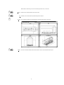
This program starts with the following window:
clicking on "Load Materials" a new window will pop up:
Here we can see the names of the materials and their coefficient
can be resized using the standard Windows procedures.
49
α , for each octave.
This window
α
R
Update File
Quit
Absorbing factor. Pressing this button every absorbing factors of each band will be displayed.
Phonoinsulating coefficient. Pressing this button the coefficients of each band will be displayed.
Saves the work done until this moment.
Exits the program with the following dialog box:
If you want to insert a new material you should position the cursor on an empty line and press the left
arrow (ï). Then you’ll insert the material name and all of its parameters
50
7.
Source Manager
51
7.1.
File Menu
New
Open...
Creates a new source data file.
This command opens the common open dialog:
where you can load any .SPK file previously generated by Source Manager.
Save
Save As
This item saves the work done, if you haven’t saved it before you’ll prompted for a new file name with
the Save As... dialog box.
This command allows you to save the file with a given name:
52
Import
Source (BZ)...
This command imports Modeler 3.0 or Modeler 3.1 speaker files:
This item will pop up the following dialog box:
These BZ curves describe the directivity of a source. You should specify if you want to create a
sound or noise source with the “Sound source type” radio button. Now you have to select a BZ curve
for each band (BZ1, BZ2, ..., BZ10).
%
.
Y OU CAN ASSIGN A “0” POWER VALUE ONLY TO THE FIRST BANDS OR TO THE LAST ONES. Y OU CAN’T LEAVE POWER HOLES OTHERWISE THE PROGRAM WILL
CRASH
53
If you have selected a “Noise Source” you’ll see this dialog box:
where you can specify the linear power level in dB of the source. If you have selected “Loudspeaker”
you’ll be asked for the electric power in Watt. The program will distribute the energy for each band
automatically. Now you can press “OK” an save the work with the Save as... menu item.
Source ISO 3744...
If you know the sound pressure level according to the ISO 3744 (3746) standard you can describe a
source with the following dialog box:
You must insert the power levels for each band in dB, the dimensions of the parallelepipedal surface
in meters and the room volume where the measures were taken. When you’re done, click on the “OK”
button to see the next dialog box:
54
where you can specify the source name and manufacturer.
If you select the “Load from file” item you can load .DAT or .PRN files with this dialog box:
“Save to File” button will show the common Save dialog box:
55
Clicking the “Display Lw“ you can see the power level spectrum for each octave, linear and A
weighted of the source you’ve just created.
Obviously “Print Window” will dump the window to the current printer.
There are also other methods to specify a source: parallelepipedal surface with 5 microphones,
conformal surface with 8 microphones and hemispherical surface with 10 microphones.
56
57
In all these cases you can follow the same procedure described above, the only variation is the
number of required parameters.
Auto Print Screen This command prints the current window.
Printer Setup
Exit
This item allows you to select and set the current Windows printer.
This command exits the program.
58
7.2.
Edit Menu
Cut
Copy
7.3.
This command puts in the clipboard the current selection and deletes it.
This command puts into the clipboard the current selection.
Paste
This command pastes in the current position the contents of the clipboard.
Delete
This command deletes the current selection
View Menu
Balloon
This command displays the following window:
that shows the directivity balloon for the frequency selected in the listbox.
When you can’t see any balloon the corresponding frequency has no power emission.
59
Curves (2)
This command shows the following situation:
where the horizontal and vertical radiation diagram of the specified frequency are displayed.
Curves (All)
This command fills the main window in this way:
These 18 windows show the planar radiation diagrams of the selected frequency with planes rotated
with a step of 10° with respect to the horizontal plane.
60
Header Selecting this command you’ll get the following dialog box:
where you can insert the source and manufacturer name, the first and last significative frequency.
Info
Displays a window with general information about the current source:
Here we can see the source type, the sound power level in dB, the directivity, the sensitivity, the
electric impedance and the efficiency.
Data
This command displays the directivity coefficients of each point of the balloon for the selected
frequency:
61
Standard
7.4.
This command opens the following 5 windows:
Window Menu
Cascade
(Shift+F4) This command presents the typical Windows behavior:
62
Tile
Arrange Icons
Iconize All
Deiconize All
Close All
(Shift+F5) This command fills the main window with all the active child windows, as usual in Windows
environment.
Arranges all the iconized windows at the bottom of the main window.
Iconizes all open windows.
Inverts the effect of the previous command.
This command closes all the active windows.
Clear Screen Clears all the screen from previous messages.
63
7.5.
Help Menu
Index...
This commands displays the help index.
About...
Displays the window containing information on the program and its authors.
64
8.
Ramsete Trace
65
This program starts with the following dialog box:
Level
It’s the level of source balloon subdivision: the number of pyramids will be 8x2N where N is our
inserted value.
Time
It’s the duration of the tracer analysis: it should be as near as possible to the reverberation time in
seconds.
Precision
Is the width of each sample of the impulse response. It can assume any positive value but normally
it ranges from 0.001 (theaters) to 0.1 (factories).
History
Is the number of reflections before a pyramid is ignored: a zero value instructs the program to
compute the direct wave only; a negative value tells the tracer to ignore this parameter and to follow
the pyramids on a time basis.
Humidity
It’s the relative air humidity. The default value is 80%.
%
THE LEVEL, T IME AND HISTORY VALUES HEAVILY INFLUENCE THE COMPUTATION TIMES:
•
Level EXPONENTIALLY ;
•
Time LINEARLY ;
•
History LINEARLY .
WE HAVE ALREADY STATED THAT THE COMPUTATION TIME IS STRONGLY
SOURCES AND RECEIVERS.
%
TIED UP TO THE NUMBER OF SURFACES IN THE GEOMETRIC MODEL AND THE NUMBER OF
THE TIME AND P RECISION PARAMETERS, THE NUMBER OF RECEIVERS INFLUENCES LINEARLY THE DIMENSION OF THE RESULTS FILE .
66
Save
Cancel
About
This button save the current values and uses them as a default in the next working session.
Will exit the program.
Will display the following about box:
During the tracing process the following status window will be displayed:
When the computation of a source has been completed the relative results will be saved in a file with
an extension named after the letter associated to the source by Ramsete CAD: .__A for the first
source, .__B for the second and so on.
Pressing “Cancel” you’ll abort the computation of the current and subsequent sources but the result
files of the preceding ones won’t be deleted.
%
BEFORE LAUNCHING A LONG ELABORATION GET SURE THAT ALL WINDOWS SCREEN SAVERS ARE DISABLED: THEY CAN HOG THE CPU FOR A WORTHLESS
. I F YOU HAVE TO WAIT MANY HOURS, IT’S MUCH BETTER TOTURN THE MONITOR OFF
TASK SLOWING DOWN THE PYRAMID TRACE UNACCEPTABLY
67
9.
Ramsete Graph
69
This is the opening screen:
when you open a file with the standard Windows procedure you’ll get this status window:
The Alfa and Beta constants are used for fine tuning the reverberation queue and shouldn’t be
changed. You can directly edit them in the ramsete.ini file but we don’t recommend that, on the
contrary we suggest to use more than 8 subdivisions in Ramsete Trace.
When you press “OK” you get a toolbar similar to this one:
In the first row you can see the list of the receivers and their mean labeled as “R” that stands for
room data. The room receiver has not a real position in space, so it has only a symbolic meaning, not
deterministic like other receivers.
In the second buttons’ row you can see all frequency bands and their linear and weighted A sum:
When you open the impulse response window, you’ll get the information about the currently selected
receiver and frequency.
70
9.1.
File Menu
Open...
Sum...
This command allows you to select a file generated by Ramsete Trace and load it:
This commands allows the selection of more than one file generated by the same geometric model
but from different sources. The first step consists of the selection of any data file in order to specify
the name of the model:
In the second phase you should select the sources you want to add together:
71
When you have done the selection, a new file with extension .___ will be created. Later you can load
this file alone or to sum it to other data files, in this case we suggest to rename it using the Windows
File Manager as usual.
Print
About...
Will send to the printer the current window.
Will show some information about the program and its authors:
72
Exit
9.2.
Edit Menu
Copy
9.3.
Quits the program.
Put in the clipboard the contents of the current window in text form, so that you can paste them into
any spreadsheet application (such as Microsoft Excel or Borland Quattro Pro.
Chart Menu
Impulse Response
This command displays the impulse response at specified frequency of the current receiver:
You can click anywhere in the window in order to move the cursor, represented by a vertical line, and
display in the bottom left corner the level in that precise point. You can move the cursor using the
arrow keys too.
If you keep the mouse button pressed you can draw a rectangular area and zoom the graphical
representation of the curve. If you want to come back to the normal scale you have to press the right
mouse button.
73
Schroeder This item will show the backward integration of the impulse response using a method developed by
Schroeder:
The cursor can be moved in the same way as described above ($ Impulse Response).
SPL
This command will pop up a window with frequency response of the selected receiver for each
octave, linear and weighted A:
%
THE CURRENTLY SELECTED FREQUENCY IS OBVIOUSLY IGNORED IN THIS CASE.
74
T10
This command displays the T 10 decay time chart.
T15
This command displays the T 15 decay time chart.
T20
This command displays the T 20 decay time chart.
T25
This command displays the T 25 decay time chart.
T30
This command displays the T 30 decay time chart.
T60
This command displays the T 60 decay time chart.
Autoresize
9.4.
This command enables or disbles the automatic computation of the minimum and maximum values
in charts in order to resize them accordingly.
Table Menu
In this menu all commands display a table containing data for each receiver and frequency, so the
current selections are not influent.
75
SPL
This command displays the SPL table.
T10
This command displays the T 10 decay times table.
T15
This command displays the T 15 decay times table.
T20
This command displays the T 20 decay times table.
T25
This command displays the T 25 decay times table.
T30
This command displays the T 30 decay times table.
T60
This command displays the T 60 decay times table.
EDT
This command displays the Early Decay Times table.
LFC
This command displays the LFC table.
LC
This command displays the LC table.
LE
This command displays the Lateral Efficiency table.
76
9.5.
Window Menu
Cascade
Will put all the open windows in a cascade:
Tile
Will fill the main window with all the current charts and tables.
Arrange Icons
Will align all the iconized windows at the bottom of the screen.
Close All
Will close all the active windows.
77
10. Ramsete View
78
This is the opening window:
Let’s describe the tools on the bottom line.
Focal Length This spin button contains the focal length of the imaginary camera you are using to take a picture of
the geometric model.
Camera position
Target position
Redraw
It’s the position in space of your camera.
It’s the point you are aiming at.
Updates the view (takes the photo).
You can also turn your camera left or right side using the horizontal scroll bar, on the contrary you
can use the vertical scroll bar to move the camera up and down.
10.1. File Menu
Open Geometry File
This command opens the common Open file dialog box:
79
Here you can select any Ramsete CAD file in order to display it without computing any acoustic
parameter.
Save Geometry File
This command opens the common Save file dialog box:
This option can be used to save geometric models in .RAY format when they have been loaded from a
.DXF file.
DXF In...
This command imports .DXF files, so that you can convert them in .RAY files with the previous
command.
80
DXF Out...
Response+Geometry File
This option can be used to save geometric models in .DXF format when they have been loaded from a
.RAY file.
This command opens the common Load file dialog box:
Ramsete view can handle two different file formats: Ramsete Trace ASCII text format or its binary
format. When you load a Ramsete Trace file it’ll be saved in binary format in order to speed up any
subsequent processing. This command loads both the geometry and the impulse responses
computed by Ramsete Trace in order to reach high quality graphic outputs such as perspective
mappings of the room. When loading process has finished, you’ll se the dialog box for the
computation of the Speed Transmission Index ($ STI Options...):
81
Auto Print Screen...
Printer Setup...
Exit
This command prints the current window.
Will pop up the common printer setup window.
Quits the program.
10.2. Edit Menu
Copy to Clpbrd
This command copies the current window into the Windows clipboard.
10.3. View Menu
Draw 3D
When you load a geometric model you get a window like this one:
where you can have a perspective view of the model from any point of view ($ introduction of this
chapter)
82
Draw 2D
Displays a plant view of the model:
Here you can only change the focal length or panning the window using the horizontal or vertical scroll
bars.
Render...
View Options...
Launches the Render program, described in the next chapter ($ Render).
Opens a dialog box where you can select the entities to display or hide and their colors.
83
Auto Redraw
View Room
View Sources
View Receivers
This check box toggles the status of the button on the right side of the main window. In “Auto
Redraw” mode all changes to the “Focal length”, “Camera Position” and “Target Point” cause an
immediate update of the screen, otherwise you have to press “Redraw” each time you’d like to take
the picture.
Shows or hides the room geometry.
Shows or hides the sources.
Shows or hides the receivers.
View BLNs
Activates the blanking file if loaded.
View Axes
Shows or hides the axes.
Post Values
Displays the numeric value of the mapped parameter close to each receiver.
If you click on the colored region of each option, you can choose the color of the corresponding entity
with this dialog box:
If you want to define a custom color you can press the proper button and open the common color
selection dialog:
84
10.4. Map Menu
Load response file
Opens the common open file dialog box:
Here you can select an impulse response without the corresponding geometry ($ Open
Response+Geometry File).
When the loading process has been completed, you’ll se the dialog box for the computation of the
Speed Transmission Index ($ STI Options...):
Mapping Options...
Allows you to specify all mapping options in this dialog box:
Parameter This list box selects the parameter to map, it can assume the following values:
•
•
•
•
SPL
Ldir
Lrev
R/D
Sound Pressure Level
Direct Wave Level
Reverberated field level
85
Actual Frequency
•
•
•
•
•
•
Lp-Lw
C50
C80
Tbar
Aeq
STI
•
•
•
LE
Aeq2
ITDGeq
Dresda Group
Dresda Group
Cremer, Kürer
Ando
Houtgast & C
Jordan
Initial Time Delay Gap
Beranek
It’s the frequency for the current parameter, it can assume these values:
•
•
•
•
•
•
•
•
•
•
•
•
Color Scheme
Klarheitsmass
Klarheitsmass
Barycentrical Time
Equivalent Reflection Amplitude
Speech Transmission Index
(RASTI is the A weighted of STI)
Lateral Efficiency
31.5
63
125
250
500
1000
2000
4000
8000
16000
Lin
A
Selects a standard color combination:
•
•
•
•
•
•
Blue-Red
Green-Red
White-Blue
White-Black
R-G-B
Iris
Min. Level
Defines the lowest value for the current parameter.
Max. Level
Defines the maximum value for the current parameter.
These values are automatically computed, but you can change them manually in order to get a better
dithering of a critical parameter value.
X divisions
Defines the number of horizontal steps of the Surfer grid.
Y divisions
Defines the number of vertical steps of the Surfer grid
This parameters are passed to the Surfer program that computes the mapping of the parameters.
The higher they are the nicer the mapping will look like, but you can’t exceed the limits of available
DOS memory.
86
3D Z value
Defines the Z coordinate of the perspective mapping plane ($ Do Dither 3D...). This value should
be equal to the height of the receivers, normally 1.7 m.
Increment
It’s the step between two isolevel curves.
Use Surfer
If you purchased Surfer you can also check this box, otherwise you have to use a simpler mapping
procedure.
Max. Radius
Use Blanking file
The research radius of this latter algorithm can be specified in this edit box.
This checkbox let you use a blanking file if you want to use the Surfer program ($ Blanking menu),
the file name can be specified in the following dialog box:
View Options
Recalls the view options dialog ($ View Options...).
STI Options...
When you load an impulse response file you’ll always see this dialog box:
where you are asked if the background noise can be ignored or not. If you click on the “Present”
radio button, you need to specify the noise SPL for each band in the next dialog box:
87
RGB Options...
This commands allows you to specify one by one the colors used for the gradient mapping:
If you click onto a colored box you’ll be prompted with the color selection dialog box ($ View
Options).
88
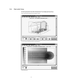
Do Dither 3D...
This command shows the “Mapping options” dialog box ($ Mapping Options) and starts the
Surfer program. When you can hear a beep you realize that the program has finished its
computation and you will see a perspective mapping of the selected parameter using all options
specified with the “View options” and “Mapping options” dialog boxes:
Do Dither 2D...
This command is very similar to the former one in usage, obviously you’ll get a bidimensional
mapping of the selected parameter:
89
Do Contour 3D...
This command performs the same steps of the previous commands and outputs a perspective
mapping of isolevel curves of the selected parameter.
Do Contour 2D...
This command is similar to the previous one, but it displays a bidimensional mapping like this:
90
10.5. Blanking Menu
The blanking procedure defines the mapping area precisely in order to reach better graphical results
also with a small number of grid subdivisions ($ Mapping Options).
Clear
Load...
Add Line...
Deletes the polygonal region from the screen.
Loads a previously saved blanking file with a .BLN extension:
When you select this command you must insert the following value:
If your answer is “0” the mapping will take place inside the polygon that you’ll draw, otherwise it will
be blanked inside of it. At this point a small 2D CAD system will switch on to allow you to insert the
polygon vertices. In the bottom line you can see the current cursor position.
91
Save...
%
Y OU SHOULD BLANK ONLY AREAS THAT DON ’T CONTAIN RECEIVERS.
%
THE BLANKING POLYGON SHOULD ALWAYS BE CLOSED.
This command saves the work performed with the common save dialog:
This file can now be used in the “Mapping Options” dialog box ($ Mapping Options).
92
10.6. Surfer Menu
Grid...
Activates the Grid subprogram of the Surfer package.
Topo...
Activates the Topo subprogram of the Surfer package.
Plot...
Activates the Plot subprogram of the Surfer package.
Set Plotter...
Activates the Plotter subprogram of the Surfer package.
10.7. Help Menu
Help...
About...
Opens the help file.
Displays some information about the program version and its authors:
93
11. Render
94
11.1. File Menu
Exit
Quits the program.
11.2. View Menu
Redraw
Set Lighting...
This command redraws the entire screen.
This command opens the following dialog box:
where you can edit the RGB values of “ambient light”. These values range from 0,0,0 (black) to
65535, 65535, 65535 (white), while the default values are 32767, 32767, 32767 (gray). The
“Level” parameter represents the luminous intensity and can range form 0.0 to 1.0
The “Lighting” menu allows you to specify the parameters of four spot lights with the following dialog
box:
Here you can also point the location and the target point of the spot source. The “Shape” value can
range from 0 to 1 and represents the concentration of the light beam.
95
Set Camera...
Lens
Roll Angle
From
To
Set Back Color...
Using this command you can set the camera parameters:
It’s the focal length.
It’s the angle of rotation of the camera with respect to the ground: 0.0 for landscape; 90.0 for
portrait.
It’s the camera position.
It’s the target point.
Allows you to specify the background color:
This dialog has been described in the View Options command ($ View Options).
96
11.3. Rendering Menu
Wireframe
Shows a wireframe representation of the model:
Painter Render This option shows a flat shade of the geometry using the painter algorithm:
97
ZPoly Render
This option computes also different color shades inside the same face:
ZBuffer Render This algorithm is much slower but gives more realistic results:
98
11.4. Output Menu
File Name...
Saves a file containing the current displayed image:
Metafile (Winword) .APM Selects a .APM Metafile.
Bitmap (Pbrush) .BMP
Selects a standard Windows .BMP file.
Do File Output!
This button creates the desired file.
Copy to Clpbrd
Copies into the clipboard the current window.
11.5. Help Menu
Render Help...
About...
This option loads the Render help file.
This command opens Ramsete View about box:
99
12. Troubleshooting
When you get a warning box telling you “Hey you forgot to connect the dongle”, you probably forgot to
connect the hardware protection key to your computer. If you have properly connected the dongle
and the problem still remains one of these assertions may be true:
The printer connected to the same parallel port is off;
There is a parallel cable without any printer at all on the other side
The hardware protection or the parallel port are faulty.
12.1. Ramsete Trace
If Ramsete Trace presents some escaped rays please check carefully the geometric model in order
to verify that it is well closed.
When Ramsete Trace can’t find a sound source you have to verify that it’s still placed in the same
directory where Ramsete CAD found it. In this case you have to edit the .RAY file manually or put the
source in the original directory.
If the computation times are longer than usual check the specified tracing parameters and have a
look at the “Turbo” indicator of your machine.
12.2. Ramsete Graph
If Lp > Lw the receiver is too near to a sound source (less than 1 m).
If the program displays a sound pressure level that’s half of the expected value you should check the
position of the source, it could be exactly on a wall.
12.3. Ramsete View
For a correct mapping computation you should select the point as a decimal separator (not the
comma!) in the Windows Control Panel.
101