Download RiSCAN PRO

Version 1.2.0sp1
RiSCAN PRO
© 2005 - Riegl LMS
All rights reserved. No parts of this work may be reproduced in any form or by any means - graphic, electronic, or
mechanical, including photocopying, recording, taping, or information storage and retrieval systems - without the
written permission of the publisher.
Products that are referred to in this document may be either trademarks and/or registered trademarks of the
respective owners. The publisher and the author make no claim to these trademarks.
While every precaution has been taken in the preparation of this document, the publisher and the author assume no
responsibility for errors or omissions, or for damages resulting from the use of information contained in this document
or from the use of programs and source code that may accompany it. In no event shall the publisher and the author be
liable for any loss of profit or any other commercial damage caused or alleged to have been caused directly or
indirectly by this document.
Printed: July 2005.
Contents
I
Table of Contents
Foreword
0
Part I Introduction into RiSCAN PRO
5
Part II Installation
7
1 System requirements
................................................................................................................................... 7
2 Program installation
................................................................................................................................... 7
3 License manager
................................................................................................................................... 10
Part III Getting started
14
1 Main program
...................................................................................................................................
window
14
2 Program settings
................................................................................................................................... 24
3 Coordinate systems
................................................................................................................................... 30
4 Create new project
................................................................................................................................... 32
Project settings
.......................................................................................................................................................... 33
Create new scanposition
.......................................................................................................................................................... 35
5 Calibrations ................................................................................................................................... 36
Camera
.......................................................................................................................................................... 36
Camera model
......................................................................................................................................................... 37
Camera calibration
......................................................................................................................................................... 40
Base camera calibration
......................................................................................................................................... 42
Based on reflector
.........................................................................................................................................
column
42
Based on flat check
.........................................................................................................................................
pattern
48
Based on reflector
.........................................................................................................................................
array
56
Field of view
......................................................................................................................................................... 59
Tiltmount
.......................................................................................................................................................... 59
Part IV Data acquisition
65
1 Scan acquisition
................................................................................................................................... 65
Overview scan
.......................................................................................................................................................... 69
Panorama scan
.......................................................................................................................................................... 70
Inclination sensors
..........................................................................................................................................................
(optional)
71
Reflector extraction
.......................................................................................................................................................... 73
2 Image acquisition
................................................................................................................................... 74
Reflector extraction
.......................................................................................................................................................... 77
3 Tiepointlist window
................................................................................................................................... 78
4 Tiepoint scans
................................................................................................................................... 90
Part V Data visualisation
95
1 Viewtypes
................................................................................................................................... 95
2 2D view
................................................................................................................................... 96
General
.......................................................................................................................................................... 97
Navigation .......................................................................................................................................................... 100
© 2005 - Riegl LMS
I
II
RiSCAN PRO
3 3D view
................................................................................................................................... 102
Object view .......................................................................................................................................................... 102
Navigation .......................................................................................................................................................... 105
Object inspector
.......................................................................................................................................................... 108
Toolbars
.......................................................................................................................................................... 117
Viewports .......................................................................................................................................................... 118
4 Readout window
................................................................................................................................... 118
5 Tiepoint display
...................................................................................................................................
window
121
6 Image browser
...................................................................................................................................
window
122
Part VI Data registration
125
1 Registration...................................................................................................................................
via tiepoints
125
2 Registration...................................................................................................................................
via inclination sensors (optional)
130
3 Manual coarse
...................................................................................................................................
registration
131
4 Backsighting
................................................................................................................................... 136
5 Registration...................................................................................................................................
of project images
139
6 Hybrid multi...................................................................................................................................
station adjustment
141
Part VII Data postprocessing
143
1 Data manipulation
................................................................................................................................... 143
Select
.......................................................................................................................................................... 143
Actions on selected
..........................................................................................................................................................
data
144
Filter
.......................................................................................................................................................... 145
Clean
.......................................................................................................................................................... 147
Resample .......................................................................................................................................................... 148
2 Triangulation
................................................................................................................................... 150
Triangulation
..........................................................................................................................................................
of a scan
151
Triangulation
..........................................................................................................................................................
of arbitrary point clouds
153
Triangulation
..........................................................................................................................................................
of a plane
155
3 Working with
...................................................................................................................................
meshes
155
Smooth & decimate
.......................................................................................................................................................... 155
Texture
.......................................................................................................................................................... 161
4 Create Orthophotos
................................................................................................................................... 164
Orthophoto ..........................................................................................................................................................
plugin
165
CityGRID Ortho
..........................................................................................................................................................
plugin
168
5 Create geometry
...................................................................................................................................
objects
170
Point
Polyline
Sphere
Plane
Sections
Tiepoint
.......................................................................................................................................................... 171
.......................................................................................................................................................... 171
.......................................................................................................................................................... 173
.......................................................................................................................................................... 173
.......................................................................................................................................................... 176
.......................................................................................................................................................... 177
6 Measurements
................................................................................................................................... 177
Measure point
..........................................................................................................................................................
coordinates
178
Measure distance
.......................................................................................................................................................... 178
Measure volume
..........................................................................................................................................................
and surface
180
7 Animations................................................................................................................................... 184
© 2005 - Riegl LMS
Contents
III
8 Panorama images
................................................................................................................................... 187
Part VIII Data exchange
1 Import
190
................................................................................................................................... 190
ASCII
.......................................................................................................................................................... 190
Documents .......................................................................................................................................................... 191
Aerial views.......................................................................................................................................................... 191
2 Export
................................................................................................................................... 191
3PF
DXF
OBJ
POL
VRML
STL
PLY
.......................................................................................................................................................... 192
.......................................................................................................................................................... 192
.......................................................................................................................................................... 193
.......................................................................................................................................................... 193
.......................................................................................................................................................... 193
.......................................................................................................................................................... 193
.......................................................................................................................................................... 193
3 Fileformats................................................................................................................................... 194
3DD
.......................................................................................................................................................... 194
3PF
.......................................................................................................................................................... 194
COP, SOP, POP
.......................................................................................................................................................... 195
DAT
.......................................................................................................................................................... 196
ROT
.......................................................................................................................................................... 196
RSP (Project..........................................................................................................................................................
file)
197
UDA
.......................................................................................................................................................... 197
VTP
.......................................................................................................................................................... 197
World file .......................................................................................................................................................... 197
ZOP
.......................................................................................................................................................... 198
Part IX Appendix
202
1 Download information
................................................................................................................................... 202
2 Abbreviations
................................................................................................................................... 202
3 Angle definition
................................................................................................................................... 203
4 Program shortcuts
................................................................................................................................... 203
5 RiPort
................................................................................................................................... 205
6 RiSCANLIB................................................................................................................................... 206
7 Copyright remarks
................................................................................................................................... 207
VTK
.......................................................................................................................................................... 207
8 Revision history
................................................................................................................................... 207
Index
218
© 2005 - Riegl LMS
III
Part
I
Introduction into RiSCAN PRO
Introduction into RiSCAN PRO
1
5
Introduction into RiSCAN PRO
RiSCAN PRO is the companion software package to the RIEGL 3D laser imaging sensor of the LMS-Z series. It
allows the operator of the 3D imaging sensor to perform a large number of tasks including sensor configuration,
data acquisition, data visualization, data manipulation, and data archiving using a well documented structure.
RiSCAN PRO is project oriented. All data of a project is stored within a single directory structure containing all
scan data, calibrated photographs, registration information, additional descriptors and processing outputs.
We publish our project structure to allow our software partners to directly access all useful data gained within a
scan project. The structure of the project is stored in a text based- and documented project file making use of the
XML language (see "Data exchange: Fileformats: RSP 197 "). The name of the project file is "project.rsp". Within
RiSCAN PRO all data is organized in a tree structure for comfortable access and clarity.
(c) 2005
Part
II
Installation
Installation
2
Installation
2.1
System requirements
7
Before you install RiSCAN PRO on your PC please make sure that the system meets the following requirements:
Operating system:
Windows 2000, Service Pack 2 or above
Windows XP (Professional recommended)
Memory requirements:
256 MB RAM minimum,
1024 MB or more recommended
Disk space requirements:
approximately 30 MB for the program
approximately 700 MB for the example project (only included in the CD version of RiSCAN PRO)
at least 40 GB recommended for own projects
Interface for scanner communication:
Serial and ECP parallel interface or alternatively ethernet (LAN) interface
Graphics requirements:
OpenGL accelerated graphics card
nVIDIA GeForce series recommended (GeForce2 or better)
Peripherals:
3 button mouse, optical wheel mouse recommended
2.2
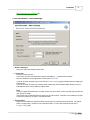
Program installation
To install RiSCAN PRO on your system just run "SetupRiSCAN_PRO.exe".
This program will guide you through all parts of the installation process.
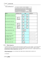
Steps of installation:
·
License - agreement:
At first of all you will be prompted to accept the license - agreement.
Press on the button "I agree" in order to accept the license and continue the setup.
Otherwise the setup will be aborted without installing RiSCAN PRO.
·
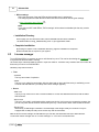
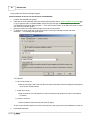
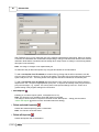
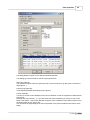
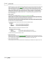
Component selection:
(c) 2005
8
RiSCAN PRO
At this dialog it is recommended to select the "Full Install" option to make sure that
all components will be installed.
Component description:
· RiSCAN PRO (required)
The application itself
· Default program settings
This option is only of interest when you update RiSCAN PRO to a newer version. Disable this option to
keep your program settings. Otherwise they will be overwritten with default values.
· Default project
Contains a RiSCAN PRO project with default camera calibrations and camera mountings.
The default project will be copied to the selected project folder which will be defined on the next page.
· Startmenu shortcuts
Add shortcuts (links) for RiSCAN PRO to your startmenu.
· RiPort
This installs the RiPort driver on your system.
Note: RiPort is not needed on PCs with MS Windows95/98 or if you do not intend to use the parallel
port for data acquisition.
If setup detects that RiPort is already installed, you will be asked whether the installed driver or the
driver of the RiSCAN PRO package should be used.
If you decide to use the driver of the package, the old driver is deinstalled and the new driver is
installed.
Note: This will result in rebooting the system twice.
(c) 2005
Installation
9
More information about "RiPort" 205
·
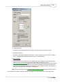
User information / RiPort settings:
· Name & Company:
Enter your name and company name here.
· License key:
Enter the license key here.
The license key can be entered with or without the dashes ( "-" ) between the numbers.
Also the characters can be uppercase or lowercase ( "A" or "a" ).
If you do not enter a license key you can use the license manager 10 of RiSCAN PRO to manage your
licenses later.
If you do not enter a license key a default viewer license key will be installed which allows you to run
RiSCAN PRO but you are not able to acquire data.
Note:
If you just update RiSCAN PRO to a newer version you do not have to enter a license key because the
"old" one(s) are taken.
The license keys of RiSCAN PRO are saved in a per-user manner. Therefore every windows user has
to enter the license key in order to run RiSCAN PRO.
· Project folder:
Enter the folder where the projects and the default project (if selected) should be saved. The default
folder is "Riegl Scans", located in your documents folder. You can also modify this folder in the
Program settings 24 .
(c) 2005
10
RiSCAN PRO
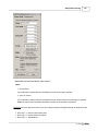
· RiPort settings:
Select the port name of the new RiPort and the parallel port it is assigned to.
The setup-program will install the RiPort-Driver and add a new RiPort with the given settings.
-> More information about "RiPort" 205
Note:
If you select to NOT install RiPort, "RiPort settings" will be shown but disabled (the lists only contain
"not used").
·
Installation Directory
On this page you can choose the folder, where RiSCAN PRO should be installed to.
The default folder is "Riegl_LMS\RiSCAN_PRO\" in your applications folder.
·
Complete installation
By clicking on "Install" on the "Installation Directory" page the installation is completed.
Now all needed files are copied on your system.
2.3
License manager
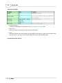
To run RiSCAN PRO it is necessary to enter a valid license key once. This can be done during the installation 7
or anytime while RiSCAN PRO is running.
The license keys of RiSCAN PRO are saved in a per-user manner. Therefore every windows user has to enter the
license key in order to run RiSCAN PRO.
Generally a key has two criteria:
· Time
- unlimited
This key has no date of expiration.
- limited
This key is only valid till a certain date. After this date (and no other valid license key is available) you can
not work with RiSCAN PRO. (On startup the license manager appears.)
· Device
- HDD-Lock
The key is only valid on a PC with a certain harddisk-ID. In this case RiSCAN PRO works with all RIEGL
LMS-scanners.
- Device-Lock
This key in only valid in combination with a certain scan device. In this case you can start the program, but
you can only work with the scanner determined by the key. Connections to other scanners will be refused.
- Dongle-Lock
Alternatively a USB dongle is available. The advantage of the dongle is that you can work on any PC
equipped with a USB port with just one license key and all instruments.
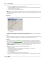
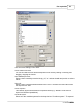
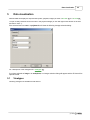
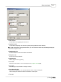
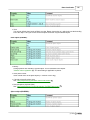
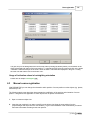
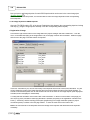
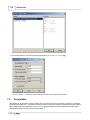
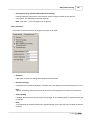
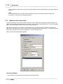
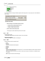
With the built-in license manager of RiSCAN PRO you can add, edit and delete licenses of RiSCAN PRO.
To show the license manager click on "License manager" in "Tool"-menu of RiSCAN PRO.
(c) 2005
Installation
11
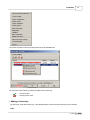
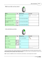
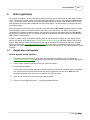
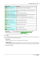
The license list shows currently existing license keys for RiSCAN PRO.
The icon near to the license key shows the state of the license key:
......... the key is valid
.......... the key is NOT valid
·
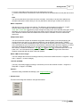
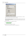
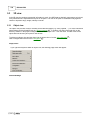
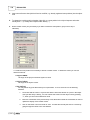
Adding a license key:
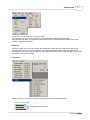
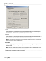
By clicking on "Add new license key" a new dialog appears, where the new license key can be inserted.
Note:
(c) 2005
12
RiSCAN PRO
It doesn't matter if you enter the license key with or without the dashes ( "-" ) and blanks ( " " ).
Also the case of the characters isn't important.
·
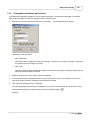
Editing a license key:
Select the license key by clicking with the mouse on it.
Click on "Edit license key".
A dialog appears, where the license key can be edited (see format notes at "Adding a license key"
·
10
).
Removing a license key:
Select the license key(s) you want to delete.
Click on "Delete license key".
The selected license key(s) will be deleted without confirmation.
·
Removing all license keys:
Click on "Delete all license keys".
Note:
There is no confirmation ("Do you really want to...")! The keys will be deleted and can not be restored.
·
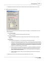
How to get the HDD-ID:
In the bottom left corner of the license manager is a box showing the HDD-ID of your PC. By clicking on the
button "Copy" the HDD-ID is copied to the clipboard in order to be used in an e-mail to [email protected].
(The HDD-ID is also shown in the "about-box" of RiSCAN PRO.)
Note:
If there is no valid license key left when you close the license manager you will be prompted to add a license the
next time you start RiSCAN PRO.
Note:
The built-in license manager of RiSCAN PRO only shows the licenses of RiSCAN PRO. To edit the license keys of
any other RIEGL LMS software product or either a plugin of RiSCAN PRO you have to use the "RIEGL LMS
License manager". You'll find this program either in the start menu in the group "Riegl LMS > Support" or in the
"Tool" menu of RiSCAN PRO. This program doesn't display whether the installed license keys are valid or not due
to security reasons.
(c) 2005
Part
III
Getting started
14
RiSCAN PRO
3
Getting started
3.1
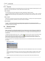
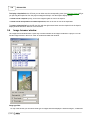
Main program window
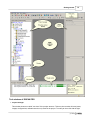
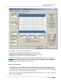
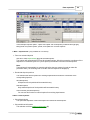
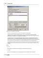
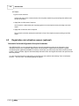
The main window of RiSCAN PRO is modular. You can decide which tool windows should be displayed and where
they should be placed. The configuration (visibility and position) will be saved on shutdown and restored the next
time you start RiSCAN PRO. The following screenshot shows RiSCAN PRO with a default configuration:
(c) 2005
Getting started
15
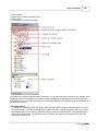
Tool windows of RiSCAN PRO
· Project manager
This window shows a so called "tree view" of the project structure. This tree view contains all items (scans,
images, configurations, calibrations and so on) saved in the project. To modify an item click with the right
(c) 2005
16
RiSCAN PRO
mouse button on the item and select your desired action from the menu.
Shortcuts (within the project manager window):
Enter
perform default action (e.g. view a scan, open the tiepointlist,...)
ALT + Enter
shows the file attributes of selected object (the standard Windows dialog will be displayed)
CTRL + Enter
open selected object in Windows explorer (file path)
F2
rename selected object
· Preview window
This window is positioned on the bottom of the project manager and shows a thumbnail of the currently
selected scan or image. You can open and close the preview window by clicking on the pin beside "Preview:".
· Message list window
This window shows all messages created by several functions of RiSCAN PRO. These messages are saved
with the project, thus you have a complete summary of all actions done in this project.
Message examples:
Project loaded, Project loaded (read only)
Project saved
Data acquisition started
Data acquisition finished
...
and also information, warnings and errors.
Note:
The number of messages in the message list is limited to 5000. Everytime this limit is reached the first
(=oldest) 1000 messages are deleted.
· Thread control window
This window shows a list of all running threads. A thread is a process which may last very long such as data
acquisition or image acquisition. These threads are running in the "background" so you may continue working
with RiSCAN PRO, although in a restricted manner. Note, that a running thread can lock items of the project
tree in order to avoid errors by changing values during the process. You can not save or close the project
neither quit the program as long as threads are running and items are locked.
· Info window
This window shows some information of the currently selected object such as number of points, file size and
so on.
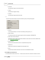
The main menu of RiSCAN PRO:
· Project menu:
(c) 2005
Getting started
17
In this menu you can load, save or close a project.
The menu item "Abort" will quit all currently running threads like data or image acquisition.
With the submenu "New" you can either create a new project or create new items (scans, views, scan
positions, images) in the project.
· Edit menu
This menu offers actions like edit, rename, show attributes, delete, and so on, that can be done on the
currently selected item of the project-window. The number and kind of actions offered depends on the
selected item. This menu is identical with the menu that appears when you click with the right mouse button
on an item of the project manager.
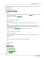
· View menu:
With this menu you can open the following windows (if they are not already opened):
·
·
·
·
Project manager 14
Message list 14
Data readout 118 (can be opened more than once)
Object inspector 108
(c) 2005
18
RiSCAN PRO
·
·
·
·
Info window 14
Thread control 14
Image browser 122
Tiepoint display 121
and the following toolbars:
·
·
·
·
·
·
·
·
·
Project management 14
Tool windows 14
Window management 14
3D - Select 143
3D - Control 117
3D - Modify 144
3D - New object 170
3D - Measure 177
Connection 14
· Tool menu:
Hybrid multi station adjustment
This menu is only visible when the HMSA-plugin is installed (see "Hybrid Multi Station Adjustment 141 ").
License manager
Shows the license manager (see "License manager
10
")
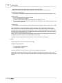
Scanner configuration
Shows the configuration dialog to configure the scanner without acquiring a new scan (see
"Scan acquisition 65 ").
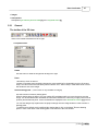
Scanner control
Shows a dialog to manually move the scanner.
(c) 2005
Getting started
19
· Move
use the bottons with the arrow to move the scanner in the resembled direction. Pressing the button
"Halt" (center) will stop the movement. Alternatively, use the following shortcuts:
"A" -> turn left
"D" -> turn right
"W" -> turn up
"S" -> turn down
· Angles
provides information about the current alignment of the scanner. Press the button "Get position" to
refresh the information.
· Align
Enter an angle for Theta (vertical alignment) and Phi (horizontal alignment) and press the button
"Align" to manually set a position for the scanner.
The button "Set park position" will reset the scanner to a defined position (Theta: 0°, Phi: 180°).
Scanner orientation
With this tool it's possible to use the optional inclination sensors of the instrument to align the instrument
(see Inclination sensors (optional) 71 ).
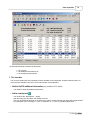
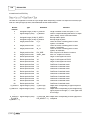
Scanner search
You can use this tool to search for an instrument connected to the same network as the PC or even if the
instrument is directly connected with the PC via a cross over network cable. This function might be useful
when you don't know the IP address of the instrument.
To search for the instrument on the complete local area network click on the button "Start search". You may
also limit the search to a fixed IP address range by clicking on "Search IP from" and entering the IP
addresses (only when no search is currently running).
All found instruments on the network will be displayed on the list in the center of the window. The columns
of the list show the IP address, the serialnumber and the name (type) of the instrument. To apply the IP
address to the communication settings of the currently opened project, select the instrument from the list
and click on the button "Apply".
Note:
The search time depends on the network speed, network load, number of network instruments connected
and the selected address range.
The button "Apply" is activated only when an instrument is selected and a project is loaded.
Repair 3DD header
To get higher accuracy some corrections are applied to the raw data measured by the instrument. These
corrections are described by a lot of parameters determined in the factory and saved in the data file gained
by the instrument (the 3DD file). In case of any misadjustment of the instrument, the point data is not
correct due to wrong correction parameters. To solve this problem it's necessary that the instrument is
recalibrated in the factory. The data files already acquired by the instrument (while it was misadjusted)
possibly can be repaired by this tool. After recalibration in the factory a template 3DD file is generated
containing a new set of calibration parameters. This template file can be applied to the faulty scan files. To
do so please proceed as follows:
· Open the project containing the faulty scan(s).
(c) 2005
20
RiSCAN PRO
·
·
·
·
Start the "Repair 3DD header" tool from the "Tool" menu.
Select the "SOURCE SCAN". This is the template scan file provided after recalibration in the factory.
Select the faulty scan files to repair.
Click on the button "OK" to start the reparation.
Note:
This function is only applicable to acquired scans (not colored or resampled) with the same type of header
(preferably the same instrument)! Furthermore it depends on the kind of misadjustment, whether you can
use this tool or not.
Media player
The built-in media player of RiSCAN PRO is able to play the following media file formats: AVI, WAV, MP3
If the playback of an video file is running (AVI) the video will be stretched/shrinked according to the size of
the window. To show the video 1:1 (100%) click on the button "Show 1:1".
Note:
Whether the media player is able to play a certain sub type of the AVI format depends on the installed video
codecs. Please contact the distributor of the video file in order to get the correct video codec.
Calculator
The calculator is a tiny tool which enables you to calculate quickly the sum or difference between two or
more values such as surface areas or volumes 180 . To add a value to the calculator just drag the value
from the project manager and drop it onto the list. To change the sign of a value, select the value from the
calculator's list and click on the button "+" or "-". On the bottom of the calculator window the result of the
calculation is displayed.
If you want to save the result click on the button with a small floppy disk on it.
Example: You want to calculate ValueA - ValueB. Proceed as follows:
· Open the calculator
· Drag ValueA and drop it onto the calculator (it gets automatically a "+" in front of it).
· Drag ValueB and drop it onto the calculator
· Select ValueB in the calculator
· Click on the button "-"
· The result is displayed on the bottom of the calculator window
To copy the result to the clipboard (e.g. in order to use it MS Excel) click on the second button from right.
(c) 2005
Getting started
21
To force a recalculation of the result click on the third button from right.
To remove a value from the list select the value first and click on the third button from left (with the red X on
it).
Note:
You can only add values of the same unit to the calculator. That means, if the first value added to the
calculator represents a surface area you can only add further values of type "surface area" and so on.
Matrix comparison
With this tool you can compare two matrices. The difference will be displayed as offset in X, Y and Z
direction and as rotation about X, Y and Z axis. To load a matrix into the tool just drag a
COP, SOP or POP matrix 202 from the project manager and drag it onto one of the both matrix grids. As an
alternative you can also click with the right mouse button into the matrix grid and select "load" from the
menu. When two matrices have been loaded click on the button "Calculate" in order to calculate the
differences.
Multiple SOP export
You can use this tool to export all orientation and position matrices (SOPs) of all scan positions of the
current project at one step (e.g. for analysis in MS Excel). On the left side of the window ("TARGET
FOLDER") you can select the destination folder (this is where all exported files will be saved). On the right
side ("scan positionS") you can select the scan positions of which the SOPs should be exported. To control
which files should be generated you can use the three boxes in the bottom right corner ("EXPORT
SETTINGS"). Possible file formats are: .SOP 195 , .DAT 196 and .ROT 196 . To start the export click on the
button "OK". For each selected scan position the files will be saved to the target folder whereas the
filename corresponds with the name of the scan position.
RIEGL LMS License manager
This tool manages the licenses for all Riegl products (it can be also reached via Start -> Programs -> Riegl
LMS -> Support -> License manager).
Terminal (RiTERM)
This tool is a terminal program for testing a connection (it can be also reached via Start -> Programs ->
Riegl LMS -> Support -> RiTERM).
Options...
Shows the dialog "RiSCAN PRO Settings" (see "Program settings
24
")
· Window menu
This menu will arrange the windows in the specified manner.
(c) 2005
22
RiSCAN PRO
· Horizontal
the windows are aligned in a horizontal manner.
· Vertical
the windows are aligned vertically.
· Cascade
the windows are aligned behind each other.
· ?
This menu will provide the help file and some wizards to guide you through the program.
· Contents
This will open the help file. It can also be reached by pressing the key "F1".
· Wizard "Startup"
This wizard will guide you through the steps for a basic configuration of RiSCAN PRO.
· Wizard "New camera calibration"
This wizard is used to create a base camera calibration used to start a new camera calibration task
(see "Base camera calibration 42 ").
· Save screenshot
this will create a screenshot and save it to a specified directory and file.
· OpenGL info
Shows some information about graphic card and graphic driver.
· About
Provides basic information about the current version and RiDRIVERs installed.
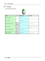
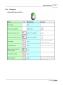
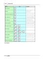
The toolbars of RiSCAN PRO
To view the different toolbars, select View -> Toolbars from the main menu and select a toolbar from the list.
(c) 2005
Getting started
23
The meaning of the different symbols and their usage will be explained in the specific documentation of the
function it is used for.
Project management:
· New
When a project is already opened, pressing the symbol will show the "New Scan
new project dialog will appear.
pressing the arrow will show the menu "New..." 14 .
65
" dialog, otherwise the
· Open
Shows the dialog to open a saved project.
· Delete selected item
Deletes the currently selected item of the project manager (scan, image, scan position, and so on).
Note:
If the trash can is activated the object will not be deleted permanently, but moved to the trash can.
To restore deleted objects, double click on the item "TRASH" in the project manager, select an object and
click on the button "undelete".
Please refer to chapter "Program settings 24 " to see how to activate the trash.
· Print
You can print a report of the current project.
· Attributes of the selected item
Shows the attributes of the currently selected item of the project window (scan, image, scan position,
tiepointlist and so on).
· Cancel
Use this button to cancel the current process (data or image acquisition).
· Help
Shows this help file.
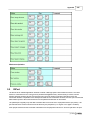
Tool windows:
·
·
·
·
·
Show
Show
Show
Show
Show
project manager 14
object inspector 108
tiepoint display 121
data readout window 118
message list 14
Window management:
(c) 2005
24
RiSCAN PRO
· Arrange windows
Use these buttons to arrange the windows horizontally, vertically or overlapped.
· Previous/Next window
Use these buttons to quickly switch to the previous or next window.
Connection:
This tool can check the network (TCP/IP) connection of the scanner and the camera server (see
"Creating a new project 32 "). For that purpose RiSCAN PRO sends a ping to the specified network address
and waits for the echo of the scanner or camera server. If an echo is received within a certain time it's
assumed that the connection is OK and a small hook appears on the button. Otherwise a small "x" will be
displayed in order to show that there's something wrong. If the tool is deactivated or it's waiting for the first
response a small question mark will appear on the button.
· Network connection state of scanner
To activate the tool click on the button with the scanner on it (the button will stay pressed).
To deactivate it click on the button again (a small question mark appears on the button).
· Network connection state of camera
To activate the tool click on the button with the camera on it (the button will stay pressed).
To deactivate it click on the button again (a small question mark appears on the button).
· Interval for network-connection-check
Click on this button to set the interval of the connection check.
Note:
This is just a simple tool to check the network connection. It only checks IF something responds to the ping
but it doesn't care WHAT responds. That means if you enter the network address of an other PC instead of
the address of the scanner, the tool would pretend that everything is OK but communication with the scanner
will not be possible unless you enter the correct address.
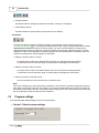
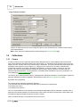
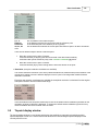
3.2
Program settings
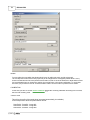
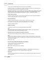
In the RiSCAN PRO settings dialog you can set several options.
·
General - Default scanner settings
(c) 2005
Getting started
Beam focus:
This beam focus is used when you select a "Overview
Increment for up/down buttons for resolution:
The value for the resolution degrees in the New Scan
here each time the arrow is pressed ( ).
69
65
", "Panorama
70
25
" scan.
window is increased/decreased by the amount set
Increment for up/down buttons for start and stop angles:
The value for the resolution degrees in the New Scan 65 window is increased/decreased by the amount set
here each time the arrow is pressed ( ).
Some older LMS Z210 instruments are not capable of high pulse-repetition-rates. Activate this option to
reduce the rate (A too high rate results in a higher number of invalid measurements).
·
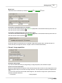
General - Image acquisition
Ask before taking image
If you will be asked before taking an image during an image acquisition, then activate this option.
Scanner movement notification
During an image acquisition the position of the instrument will be read out twice for every image taken. Once
before taking the image and once after the image was taken. The two positions will then be compared each
other.
You can choose from three options what should happens, if the deviation is larger than a specified amount
(Scanner movement tolerance):
· deactivated
... nothing happens.
(c) 2005
26
RiSCAN PRO
· warning (continue image acquisition)
· error (abort image acquisition)
·
... only a warning is printed into the message list.
... the current image acquisition will be aborted.
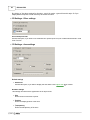
General - Optional
Some optional settings.
· General - Tiepoint scan
See Reflector extraction (Scan)
73
.
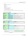
· General - Units
Define physical units used in the whole program.
Angle:
· Degree (deg)
· Radian (rad)
· Gon (gon)
Range:
· Meters (m)
· Feet (ft - 1ft = 0.3048m)
· US-Feet (ft - 1ft = 12/39.37m)
· Yards (yd)
Amplitude Scale Unit
· 0...1
· 0...255
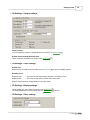
· Additional - Default viewtype
Sets the default viewtype, which is used when opening a new 2D/3D view.
(See Visualisation of data 95 )
Online preview:
Select intensity scale factor for the online preview (0..1). You can set some default values, by pressing one of
(c) 2005
Getting started
27
the "Set" buttons.
· Additional - Naming convention
You can define some default names, that will be used when a new object is created.
· Additional - Project manager
Sets several settings for the "Project window".
(See Main menu 14 )
· Additional - Recent projects and folders
Sets the initial project folder and shows the recent projects.
· New project
Sets the default settings for a new project.
· 2D Settings - Marker settings
Sets the marker style(s) of the 2D - view window.
You can set the style for each tiepoint type. This is useful when e.g. TPL SOCS and TPL IMAGE are
displayed in an image.
With "Label position:" you can select where the label (=name of the tiepoint) should be placed. This is useful,
when two tiepoints of different type (e.g. a TP SOCS and a TP IMAGE ) are at nearly the same position (Due
to the fact that the labels are on different positions, you will be able to read the names of the tiepoints).
(c) 2005
28
RiSCAN PRO
By clicking on "Use these settings for all marker - types" all marker - types will have this style. So if you
display different tiepoints in a 2D-View they will all look the same.
· 2D Settings - Other settings
Use invalid point color
Activate this option, if you want to use a defined color (Invalid point color) for invalid measurements in a 2D
view of a scan.
· 3D Settings - Axes settings
Default settings
· Show axes
Activate this option, if you want to display the axes when a new object view 102 is created.
Runtime settings
This settings will influence the appearance of all object views.
· Size
Define the size of the axes in pixels.
· Position
Define the display position of the axes.
· Transparency
Define the transparency of the axes.
(c) 2005
Getting started
· 3D Settings - Camera settings
Camera control
You can define the values for navigating with the camera in an object view 102 .
Default camera settings & Default view
These values are used when you create a new object view 102 .
· 3D Settings - Color Settings
Default color
Default colors are used when you create a new object view 102 or when you display objects.
Runtime colors
Selection color
Selected color
... This color is used when drawing selections in selection mode.
... This color is used when you have select some data.
Runtime colors influence the appearance of all object views.
·
3D Settings - Display settings
These settings are used, when you create a new object view 102 .
For detailed description of these values see the object view 102 reference.
·
3D Settings - Other settings
(c) 2005
29
30
RiSCAN PRO
Sets the default settings for a filter selection (create new orthophoto 165 ).
·
Object view settings - Control settings
Mouse
Defines the sensitivity of the mouse.
·
Object view settings - Save settings
Define how an object view should be handled.
· never save
... the object view is only temporary
· always save
... the object view is added to the project structure
· ask user to save
... you will be asked before closing the object view
·
Calculation parameters - Averaging / Resample
Set the default values for the averaging/resample-process 148 here.
If "Always ask for parameters" is checked you'll be prompted to enter the parameter each time you start the
process. Otherwise the process will start with the default values.
·
Calculation parameters - Find corresponding points
Sets the default settings for Finding corresponding points.
(See Registration of a scan position 125 )
3.3
Coordinate systems
RiSCAN PRO uses different coordinates systems, the most important ones are described below:
Scanner's Own Coordinate System (SOCS) is the coordinate system in which the scanner delivers the raw
data. Consult the user's manual of the scanner for the definition of the coordinate system. The data of every
RIEGL 3D laser imaging sensor contains for every laser measurement geometry information (Cartesian x, y, z
coordinates or polar r, , coordinates) and additional descriptors (at least intensity, optionally color information).
Thus the output of a RIEGL 3D laser imaging sensor can be addressed as a (organized) point cloud with
additional vertex descriptors in the scanner's own coordinate system.
Project Coordinate System (PRCS) is a coordinate system which is defined by the user which is for example an
already existing coordinate system at the scan site, e.g., a facility coordinate system. RiSCAN PRO requires that
all geometry data within this project coordinate system can be represented by single precision numbers (7
significant digits). For example, if mm accuracy is required, the maximum coordinates should be less than 1 km.
Global Coordinate System (GLCS) is the coordinate system into which the project coordinate system is
embedded. Usually, coordinates in the global system may contain very large numbers.
Camera Coordinate System (CMCS) is the coordinate system of the camera which is optionally mounted on top
of the scanner system providing high resolution images.
In almost all applications, data acquisition is based on taking scans from different locations in order to get a
complete data set of the object's surface without gaps or "scan shadows". The different scan locations are
addressed as scan positions. When starting a new project, i.e. starting a new data acquisition campaign, you
have to initialise a new scan position (by default ScanPos01) before acquiring data from the scanner. This scan
position will hold all data acquired at that specific setup of the scanner.
A scan position is characterized by its own local coordinate system (SOCS), i.e. the position and orientation of the
scanner within the project coordinate system. Position and orientation can generally be described by 6 parameters
(c) 2005
Getting started
31
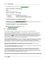
(3 for position, 3 for rotation) or by a transformation matrix. RiSCAN PRO makes use of a 4 x 4 matrix (MSOP)
addressed as SOP information (SOP for sensor's orientation and position).
The matrix consists of 9 parameters reflecting the rotation (r11 to r33) and 3 parameters for the translation (t1 to
t3). The use of homogeneous coordinates allows computation of rotation and translation in a single matrix
multiplication. The translation vector is the scanners position and the column vectors (r1i r2i r3i)T are the
directions of the local coordinate axes in PRCS. A 3D data point in homogeneous coordinates is represented by
its 3D coordinates x, y, and z by
Note:
Changing the scanners orientation at a specific location requires to use a new scan position even if the scanner
position has not changed.
Each scan position holds the scan data taken at this scan position, stored in the scanner's binary data format with
extension 3DD. Furthermore, each scan position holds its SOP information. In order to transform data from SOCS
into the project coordinate system, data points are simply multiplied with the SOP matrix (MSOP) of the scan
position.
In case a data point P has to be transformed from a specific scan position into the global coordinate system,
multiply first with the MSOP matrix of the scan position to get into the project coordinate system and multiply
subsequently with the MPOP matrix which transforms from the project coordinate system into the global
coordinate system.
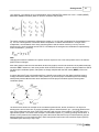
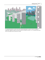
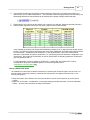
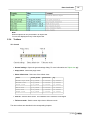
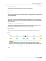
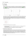
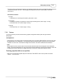
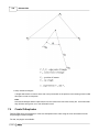
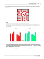
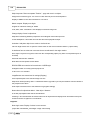
The sketch below shows an example for the coordinate systems GLCS, PRCS, and SOCS. The object is a
building scene from a bird's view. A project coordinate system is defined with the Ypr – axis being parallel to the
nave of the building and the origin of the PRCS coinciding with a corner of the building. The PRCS has to be a
right-handed system. The GLCS in the example is a left-handed system, e.g, northing, easting and elevation. A
number of scan positions are indicated by Spi, where the scanner has been set up for data acquisition (see the
detailed description on scan positions below). Each scan position has its own local coordinate system (SOCS)
resembled by the axes Xsp1, Xsp1, Zsp1.
(c) 2005
32
3.4
RiSCAN PRO
Create new project
Generally you can create a new (empty) project by selecting Project -> New -> Project... from the menu.
You will be prompted for a filename and location of the new project.
It is recommended to use the default project 7 instead of creating a "brand-new" project.
To do so, open ("Project" "Open...") the project and save it under another filename and/or folder ("Project"
"Save as...").
Using this project as a template enables you to use the existing calibrations (Camera, Mounting, Reflectors,...).
You just have to delete not needed items.
Note:
You need write permission for the target folder in order to create a new project.
The default project can not be changed because it is write protected per default.
After you have created a new project continue with the steps described in the next chapter: "Project settings
(c) 2005
33
".
Getting started
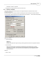
3.4.1
33
Project settings
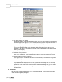
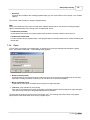
The next step is to set the project attributes.
To set the project-attributes double-click on the project-name (top most entry of the Project-manager).
The dialog "Project..." appears. The dialog has following pages:
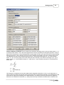
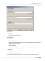
Page "General"
On this page you can insert comments like name of operator, date, location, object description and so on.
Page "Instrument"
On this page you must set the COMMUNICATION PORTS to enable communication with the instrument.
First select "Serial & Parallel" or "Network" to determine the basic way of communication, corresponding of the
type of cabelling of your instrument.
Serial & Parallel:
When "Serial & Parallel" is selected you have to select the serial port (COMx), baud rate (default is 19200)
and the parallel port (RiPTx) according to the settings of RiPORT 205 .
Network (TCP):
When "Network (TCP)" is selected you have to enter the correct IP address of the device (192.168.0.234 per
default). The ports can not be modified and are only displayed for your information. If you don't know the IP
address of the instrument you can also use the tool "Scanner Search 14 ".
(c) 2005
34
RiSCAN PRO
Note:
If you have problems while connecting to the instrument, please make sure that you have used the correct
cables. If you use a firewall please make sure that bidirectional communication over the ports displayed on
this page is allowed.
Note:
Please make sure that your PC has a valid IP address. To do so check the TCP/IP settings of the network
connection. If "obtain IP address automatically" is selected it is necessary that a DHCP server is installed in
your network. If no such server is installed (and of course when you connect the instrument directly to the PC
via a cross over cable) you have to set a fixed IP address in the same logical network IP address range as the
instrument (e.g. 192.168.0.233) and a proper subnet mask (e.g. 255.255.255.0).
Please refer to the help file of MS Windows or contact your network administrator.
On this sheet you can also set the camera type in case your instrument is equipped with a camera.
If you notice problems when connecting to your camera directly through RiSCAN PRO, please check the "USBprotocol" setting of the camera. This value must be set to "PTP" for NIKON cameras and to "normal" for
CANON cameras. For changing this setting please refer to the product documentation of your camera.
Select "Connect camera over TCP/IP" if the camera should be accessed via the network by using the camera
server (default value of Port: 20003).
Page "POP"
This page displayes the POP matrix (see "Coordinate systems
30
").
Page "Scaling correction"
To achieve maximum accuracy for the range measurement, set the atmospheric values to the actual values
during data acquisition. The GEOMETRIC CORRECTION can be entered by the user and is applied to the
measurements (ppm = parts per million).
Note: The values entered here will be the default settings for each new scan position.
(c) 2005
Getting started
35
Page "About project"
This page offers information about the project files such as location, number of files and total size of the project.
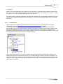
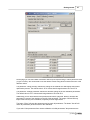
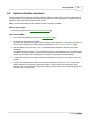
3.4.2
Create new scanposition
To create a new scan position just click with the right mouse button on the folder "SCANS" and select "New scan
position". A dialog as shown in the section below is displayed which allows you to set the attributes of the scan
position. The name of the new scan position will be set to "ScanPosXX", where "XX" is an unique number. You
can rename the scan position and give it a more meaningful name. To finally create the scan position click on the
button "OK".
scan position attributes
To modify the attributes of a scan position click with the right mouse button on the scan position and select
"Attributes...". A dialog appears showing the following pages:
Page "General"
Enter comments or a basic description here.
Page "Tilt mount"
see "Calibrations: Tiltmount
59
"
Page "SOP"
This matrix will be used to align the scan position within the project coordinate system (see
"Coordinate systems 30 ").
(c) 2005
36
RiSCAN PRO
Page "Scaling correction"
Choose an instrument from the list and adapt the values for the ATMOSPHERIC CORRECTION to ensure
exact measurements.
Note: These values are initialized with the project settings (see "Project settings 33 ").
3.5
Calibrations
3.5.1
Camera
In order to make use of the image data acquired within RiSCAN PRO you need calibration data of the camera
used. These calibration data include data on the camera itself, e.g., dimensions of the images in pixels, the focal
length of the lens, and the center of the camera image. Furthermore, you need information about the position and
orientation of the camera for every image to, e.g., apply the color of a pixel to a 3D surface. RiSCAN PRO
provides the orientation and position information "automatically" in case the camera is mounted on top of the
scanner. Up to this point the parameters describe an ideal "pin-hole" camera. However, in practice the lens
introduces significant distortion. This lens distortion is modelled within RiSCAN PRO by up to 6 parameters. For
more details see Camera model used 37 .
The camera, when ordered with the scanner, is delivered with calibration information. This information is gained by
using the calibration procedure integrated in RiSCAN PRO (usually Based on reflector column 42 ).
But please note the following:
The internal camera calibration parameters depend on
· the lens itself (even the same type of lens will lead to a different set of parameters)
· the setting of the focus
· the setting of the aperture.
Thus it is recommended to fix the camera's focus and aperture BEFORE doing the calibration. Setting the focus
depends on the intended distance the camera will be used. Please note that you always have a finite depth of the
focus which is larger the higher the aperture number is chosen.
When we tolerate blurring of 0.25 pixels we can set the focus to
(c) 2005
Getting started
37
b = 4f²/(dx a)
where f is the focal length of the lens in meters, dx is the pixel size in meters and a is the aperture number of the
lens. In this case we get "unblured" images in the range from b/2 to infinity. For example, dx = 7.8 µm, f = 14 mm,
a = 9 gives b = 11 m and an operational range from 5.5 m to infinity.
The external camera calibration parameters, especially the orientation of the camera when mounted on top of the
scanner, will be changed after detaching and mounting. To account for these changes please refer to mounting
calibrations.
3.5.1.1
Camera model
RiSCAN PRO uses a camera model similar to the one used in the "Open Source Computer Vision Library"
maintained by Intel (see http://www.intel.com/research/mrl/research/opencv/ for details).
The calibration parameters defining the camera model (intrinsic and internal parameters) are stored within
RiSCAN PRO in a tree node called CamCalib_OpenCV01 by default. A complete camera model usually includes
also external calibrations parameters defining the orientation and position of the camera in 3D space. This
information is held in RiSCAN PRO in the mounting calibration matrix, the COP matrix associated with each image
at a scan position and the SOP information of the scan position.
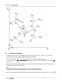
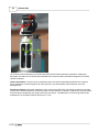
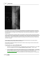
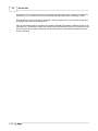
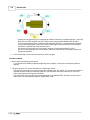
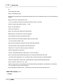
The camera model is based on a camera coordinate system (addressed within RiSCAN PRO as CMCS). The
image below shows the Nikon D100 mounted on top of a LMS-Z360 with the axes of the SOCS and CMCS. The
origin of the CMCS is the center of an equivalent pinhole camera. CMCS is a right-handed system with the x axis
pointing from left to right in the image and the y axis from top to bottom. The z axis is identical to the center of the
field of view of the camera.
(c) 2005
38
RiSCAN PRO
The camera model is described by 4 intrinsic parameters and 8 internal calibration parameters. Additionally,
descriptive information can be stored within RiSCAN PRO for documentation and data management in the field
camera information.
Camera information is not used for any computation but as the internal calibration parameters are unique for
every combination of camera specimen and lens specimen you should always make extensive use of the
descriptive text.
Intrinsic parameters reflect basic parameters of the camera chip (CCD chip). Nx and Ny are simply the number
of pixels in the horizontal direction (x direction) and the vertical direction (y direction), respectively. The parameters
dx and dy are the dimensions of a single pixel of the CCD sensor. This parameter is commonly specified by the
manufacturer, for the Nikon D100 the pixel size is 7.8 µm.
(c) 2005
Getting started
39
Internal calibration parameters can be divided into parameters describing (more or less) an ideal camera, i.e., a
so-called pinhole camera. This is the focal length and the center of projection (the orthogonal projection of the pinhole onto the chip surface). Two potentially different focal lengths (fx and fy) are used to account for the potentially
different pixel size in x and y direction and to account for different focal length's of the lens (cylindrical lens error).
The parameters fx and fy are normalized by the pixel size. The physical focal length is fx * dx. In the example
above, fx * dx is 18.3 mm, pretty close to the nominal 20 mm of the lens. The center of the image is (Cx, Cy) in
pixels. Usually, i.e., for low distortion lenses Cx ~ Nx/2 and Cy ~ Ny/2. Deviations account for a decentered lens
and/or chip.
fx......[pix]
f........focal length [m]
dx.....[m]
Lens distortion is modelled by at least two radial and two tangential coefficients, k1, k2, p1, p2, respectively. In
case k3 and k4 are both 0, the camera model is identical to the one described in OpenCV. The parameters k3 and
k4 account for higher-order modelling of the radial distortion. The details on how the parameters are applied to
transform from undistorted coordinates (i.e., ideal pinhole camera) to distorted coordinates are contained in the
(c) 2005
40
RiSCAN PRO
appendix describing the XML project file.
3.5.1.2
Camera calibration
Prerequisite for calibrating a camera is one or more images showing identifiable objects with precisely known
coordinates.
The first step to obtain a data set for calculating the model parameters is to
·
·
determine the image coordinates of the object, i.e. find the image points, and to
link the objects to the image points, i.e., to find the correspondences.
There are three different approaches that differ in the way the object coordinates in 3D are obtained and the way
the correspondences are determined. All approaches are implemented in RiSCAN PRO and are described
subsequently.
Based on reflector column
The basic idea is to set up a test field made up of a number of retroreflective targets positioned in a vertical
column in a scene when viewed by the camera. The targets should (1) cover the vertical field of view of the
camera and (2) should have a variation in depth. it is not required that the calibration field is long-term stable.
The camera to be calibrated is mounted on top of the scanner and the test field is surveyed by the laser scanner
by carrying out a number of tiepoint scans on the automatically detected targets. Then, a series of images with
flash is taken at different angular positions of the camera (automatically carried out by the calibration task). In
every image the centers of the reflectors are extracted automatically and the extracted reflectors are linked
automatically to the 3D coordinates of the targets. By this procedure, a virtual test field is generated covering in
total the complete field of view of the camera.
The major advantage is that the test field can be put up easily, no total station is required, and the calibration
task gives both the internal camera calibration parameters and the mounting calibration parameter.
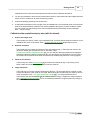
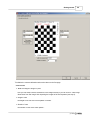
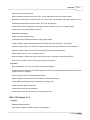
Calibration based on flat check pattern images
Especially for wide-angle lenses (for the Nikon D100 up to about 40 mm) calibration based on flat check pattern
images has been found useful. One example of an image is shown below, which shows a flat check pattern
printed on white paper used to calibrate the camera with a 14 mm lens. The size of one square is 0.1 x 0.1 m.
The check pattern is glued to a plane board to ensure the pattern is really flat.
(c) 2005
Getting started
41
For the calibration the flat check pattern is captured by the camera to be calibrated several times. The whole
image area should be covered in total, and in each image the complete pattern has to be visible. The inner
check pattern corners are detected automatically by the calibration software and are automatically linked to the
3D coordinates of the flat check pattern corners (z is always 0).
The calibration software calculates best estimates for the 10 internal parameters and for the 6 external
parameters of each image in order to minimize the deviation. The output of the calibration procedure is stored in
a CamCalib_OpenCV node within the project for further use.
With every instrument a calibration file is delivered for the camera being part of the instrument. Thus, it is not
necessary to recalibrate the camera as long as the lens parameters (focus, aperture, or specimen) are not
changed.
Calibration based on reflector array
Especially for telephoto lenses, the calibration approach based on imaging flat check patterns is inconvenient as
for a fixed focus of infinity the minimum range to the pattern has to be quite large and thus the dimensions of
the flat check pattern has to be large too. This second approach is based on imaging a field of reflectors of
known coordinates in 3D, addressed as reflector array subsequently. The reflectors must not lie in a single
plane, but have to be distributed in a volume with sufficient depth. In the example below the reflectors have
been fixed to a building to both sides of one corner and also to the roof. The reflector positions have been
surveyed by means of a total station with mm accuracy.
Assign camera calibration to images
The camera calibration can be either assigned to each image on by one (image attributes 74 ) or you can assign
the camera calibration to a couple of images at one step. To do so, please click with the right mouse button on the
camera calibration and select "Assign to images..." from the menu. In this dialog you can define several filter
settings. At the bottom of the dialog you'll see a summary of the filter settings explaining which images will be
modified in fact.
(c) 2005
42
RiSCAN PRO
3.5.1.2.1 Base camera calibration
To start with a new camera calibration task based on reflector column 42 you need an initial camera calibration.
You can either use the camera calibration of an other camera of the same type and lens or you can use the new
camera calibration wizard. This wizard allows to create an initial camera calibration based on the information
provided by the user such as camera type and type of lens. The created camera calibration doesn't contain
distortion parameters, of course.
To use the wizard please proceed as follows:
· Open or create a project.
· Click with the right mouse button on the folder "CALIBRATIONS / CAMERA" within the project manager.
· Select "New camera calibration (wizard)..." from the menu.
· Step 1: Define camera model
At this step you can either select your camera type from the list or you have to enter the camera parameters on
your own. The parameters you have to enter are the camera model (just for your own information) the number
of pixels and the size of one pixel of the image chip in both directions (vertical and horizontal).
· Step 2: Define lens model
At this step you can either select your lens model from the list or you have to enter the lens parameters on your
own. The parameters you have to enter are the lens model (just for your own information) and the focus in
millimeter.
· Step 3: Define additional data
At this step you can enter additional information such as camera settings and serial numbers of camera and
lens. Although it's not necessary to enter values at this step it is strongly recommended to do so. This makes it
easer to keep an overview which camera calibration belongs to which camera and lens.
Finally enter a name for the new camera calibration and click on the button "OK" to create it.
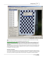
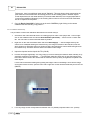
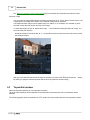
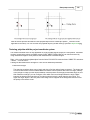
3.5.1.2.2 Based on reflector column
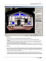
This task allows the user either to check the camera calibration or to execute the camera calibration by means
of an easy to set up calibration field.
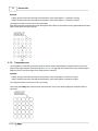
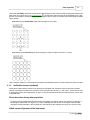
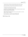
The basic idea is to have a number of retroreflective targets positioned in a vertical column in a scene. The
images below show an example of how the reflectors may be applied to existing structures, e.g., the supports of
a bridge. The targets should (1) cover the vertical field of view of the camera and (2) should have a variation in
depth, i.e., the targets should not be placed on a single plane normal to the principle axis of the camera. On the
right image the camera images is shown with the reflectors covering a vertical band of the field of view.
(c) 2005
Getting started
43
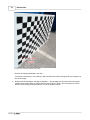
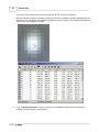
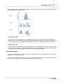
The image below shows an indoor scene with 9 reflectors attached to a column in about 3 m distance, 7
reflectors at a distance of about 8 m, and one reflector at a distance of about 13 m. The image is taken with a
flash so the targets show up clearly in the image.
(c) 2005
44
RiSCAN PRO
This calibration field alone is insufficient for accurately determining the calibration parameters of the camera.
But as the camera is mounted on the rotating part of the scanner, a sequence of images can be recorded and
all extracted targets of all images cover the complete field of view of the camera and give thus a very good
calibration field.
Usually a calibration field is surveyed by means of a total station. As the laser scanner can provide the position
of the targets in its own coordinate system very accurately by means of doing fine scans (tiepoint scans) no total
station is required. By arranging the targets as described above only few targets have been measured (in the
example above 17 targets). By taking 20 images and extracting the reflectors each provides a virtual test field
with about 340 targets.
So after setting up the test field by placing a number of targets as described above, the scanner with the
camera mounted on top is set up in front of the test field.
The procedure to extract the calibration data based on a reflector column using the scanner and the camera
mounted on the scanner is:
Creating the new camera-calibration-task
1.
Generate a new camera-calibration-task in an existing project or make a new project first. To do so rightclick on the CAMERA node and choose New calibration (reflector column) … from the menu.
2.
You are prompted to select an initial camera-calibration and a initial mounting-calibration. You can either
select a calibration from the list or import it from an other project (i.e. the default project - if copied during
the setup of RiSCAN PRO). If you have no matching camera calibration you can also use the
new camera calibration wizard 42 . These calibrations are used for initializing the task. The better these
(c) 2005
Getting started
45
calibrations are the easier the data-acquisition and thus the whole calibration task will be.
3.
You are also prompted to select a scan position where the scan, the finescans and the images should be
saved. Click on "create new" to create a new scan position.
4.
Confirm the dialog by pressing on the button "OK".
5.
A small wizard will appear on the top right corner of RiSCAN PRO. This wizard will guide you through the
steps of the data acquisition needed for the camera-calibration-task (Once you have closed the wizard
you can re-start it by right-clicking on the camera-calibration-task and selecting "Acquire calibration
data..." from the menu).
Calibration data acquisition step by step (with the wizard):
1.
Acquire new single scan
The first step is to acquire a scan of your calibration field. This scan should contain all reflectors of your
calibration field. Click on the button "Start", configure the scan as usual 65 and start the scan.
2.
Reflector extraction
The second step is to extract the reflectors of the scan made at step 1. Select the scan from the list
(should be already pre-selected) and click on the button "Start".
Configure the reflector extraction as usual 73 . The TPL SOCS of the scan position will be displayed
showing all reflectors extracted. Please open the scan and display the TPL SOCS in order to check if
all reflectors where extracted and delete all reflectors not needed (faulty detection or wrong targets).
3.
Finescan all reflectors
The third step is to make tiepoint scans 90 of all reflectors extracted at step 2. By clicking on the
button "Start" all reflectors of the TPL SOCS will be fine scanned.
4.
Image acquisition
The fourth step is to acquire images containing all reflectors. The first image will be acquired in order
to have the reflectors in the center of the image. Before taking the second image, the scanner will turn
to the next position (see "Turn angle between two images 42 "). The image aqcuisition will be
continued this way until no reflector can be extracted from the image. Configure the image acqusition
(see "Description of the input fields 42 " for more details) and start the image acquistion by clicking on
the button "Start".
(c) 2005
46
RiSCAN PRO
Description of the input fields:
· Turn angle between two images
Images will be taken in that angular distance. Either select one entry of the list on the left side or
enter the angle on the right side. The list contains some default values expressed as fraction of
the vertical field of view (FOV) of the camera (default is 1/10 FOV).
· Number of images (approx.)
This shows the approximate number of images which will be taken (Note, that this value
depends on the quality of the initial camera- and mounting-calibration and may differ from the
actually taken images).
· Sensitivity reflector extraction
With this slider you can set the sensitivity for the reflector extraction (of the images). The Range
is 0 up to 1, default is 0.5. If the images are very bright try to raise this value and vice versa.
· Number of trials (for reflector extraction)
The algorithm will try "Number of trials"-times to extract one single reflector of the image until it
fails (default is 4).
· Continue with image #
If you start the image acquisition the first time you can leave this setting as it is. If the image
acquisition was interrupted (because i.e. something got wrong during the reflector extraction,
power-loss of the camera or the reflectors where covered by something else) you can restart it
by clicking on the checkbox and selecting the number of the image which should be the next
image acquired.
5.
Calibration
After the image acquisition has finished you can calibrate the camera. To do so click on the button
"Start". The following dialog will appear:
(c) 2005
Getting started
47
On this page you can select which calculation method (least squares fitting or robust) should be used
("Figure of merit"). We recommend to use the default "robust" fitting which minimizes the sum of the
absolute values.
The parameter "Fitting accuracy" defines the change in the residual error which stops the iterative
optimization process. The default value is 1E-6. Values should range between 1E-4 and 1E-8.
The parameter "Change parameter" defines the absolute change of the ten calibration parameters.
The default value is 1E-6. Values should range between 1E-4 and 1E-8.
Additionally you can select which of the parameters should be optimized. Select or deselect the
parameter by means of the checkbox to the left of the parameter. The usage of K3 and K4 may
improve the accuracy of the calibration, especially for wide angle lenses.
The button "Clear" will reset the parameters and uncheck all parameters. The button "Use all" will
check all parameters (all will be used for the calibration.
If you select "Use parameters from camera calibration as initial parameters" the parameters are
(c) 2005
48
RiSCAN PRO
initialized with the parameters from the initial camera-calibration (Use this the first time you start the
calibration).
Finally start the calibration by clicking on the button "Start". The calibration will by started and you can
watch the progress in the "CALCULATION LOG". After the calibration has finished you can switch to
the third page "Statistics". On this page you will see a table showing all images and their mean,
minimal and maximal pixel-distances (between tiepoints of the image and the tiepoints of the scan). At
the current state an average pixel-distance about 0.5 can be considered as a good result.
To use the results in another project just import the camera- and mounting-calibration by right-clicking
on "CALIBRATIONS" and selecting "New OpenCV..." (to import a mounting: "New mounting...") from
the menu. On the following dialog click on the button "Import" to import the calibration.
Hints:
Problems during camera calibration may be based on faulty assigned camera- / mounting calibrations.
Please make sure that the correct camera- and mounting calibration is assigned to all images. Always
assign the resulting calibrations located within the calibration taskk!
3.5.1.2.3 Based on flat check pattern
To do the calibration on your own you need a check pattern. The pattern has to be as flat as possible and as
regular as possible with a high contrast. In the help directory you find a pdf file (CheckboardScaled.pdf) showing
a check pattern of 11 columns and 15 rows.
The procedure to extract the calibration data based on a flat check pattern is:
1.
(c) 2005
Generate a new node CamCalibTask in an existing project or make a new project first. To do so rightclick on the CAMERA node and choose New calibration (flat check pattern) … from the menu. The
following dialog will appear:
Getting started
49
To initialize the camera calibration task set the values on the first page:
DIMENSIONS
· Width and Height of Images in pixel
here you can either enter the dimensions of the images directly or you can click on "Take image
dimensions from first image" after importing the images of the check pattern (see step 2).
· Height of rows
the height of one row of the check pattern in meters.
· Number of rows
the number of rows of the check pattern .
(c) 2005
50
RiSCAN PRO
· Width of columns
width of one column of the check pattern in meters.
· Number of columns
the number of columns of the check pattern.
Confirm with OK. The new node is named CamCalibTask01 (the number will be increased due to existing
tasks) by default.
2.
Right-click on the node CamCalibTask01 and select Add image(s) …. Add all images taken with the
camera to be calibrated showing the flat check pattern from different view angles (take more images by
tilting and panning the camera while taking shots).
3.
The next step is to extract all crossing points (corner points of two neighbouring black fields) of the check
pattern in all images.
Open the CamCalibTask01 (double click, or right click and select "Attributes").
(c) 2005
Getting started
51
Select an image of the image list on the left side. This will load the image into the window on the right
side.
Now set two markers at the first two crossings in the first row by singleclicking with the left mouse button 100 (like the image above shows). Now you have to identify the points
through a single right-click on each marker and selecting its position from the menu (the order is not
important). If you have done a faulty assignment you can simply overwrite it by doing the assignment a
second time.
The button "Calc all crossing points" will cause RiSCAN PRO to calculate all other crossing points, which
will take, dependent on your computer configuration, more or less time. The result of the calculation will
be displayed in the image by markers.
Distorted check pattern
In some cases automated detection of corner points fails. Especially when perspective distortion yields a
ratio in width and height of the first square significantly different from 1 (compare the subsequent image).
In this case try to define the opposite square as the first square. Use again the clockwise orientation.
(c) 2005
52
RiSCAN PRO
Example for an extremely distorted check pattern
Process all images sequentially in this way.
The buttons "Cleanup ALL" and "Cleanup THIS" will delete the found crossing points of all images or of
the current image.
4.
(c) 2005
Now proceed by switching to the page "Calibration...". On this page you can select which calculation
method (least squares fitting or robust) shell be used ("Figure of merit"). We recommend to use the
default "robust" fitting which minimizes the sum of the absolute values.
Getting started
53
Additionally you can select which of the parameters shell be optimized. Select or deselect the parameter
by means of the checkbox to the left of the parameter. The usage of K3 and K4 may improve the
accuracy of the calibration, especially for wide angle lenses.
The parameter "Fitting accuracy" defines the change in the residual error which stops the iterative
optimization process. The default value is 1E-6. Values should range between 1E-4 and 1E-8.
The parameter "Focal length [mm]" helps to speed up the optimization process in case the focal length
is known.
The checkbox "Initialise all image matrices" re-calculates the position and orientation of the camera for
every image with respect to the check pattern every time you start a new fitting process. In case you
(c) 2005
54
RiSCAN PRO
have already run the fitting process once successfully and just want to see the impact of an additional
parameter, e.g., k3, on the error, de-select this option and also deselect the "Focal length" option.
Start the fitting process by clicking on the button in the lower right corner. You can watch the progress
by taking a look on the "Present fitting error".
After the calculation has been completed successfully, RiSCAN PRO displays a statistics section in the
calculation log. The statistics contains the maximum and mean distances of the real crossing points (as
specified by the check pattern parameters) transformed by means of the camera calibration data into
image coordinates.
(c) 2005
Getting started
(c) 2005
55
56
RiSCAN PRO
Furthermore, there is an additional page named "Statistics". This page shows charts representing the
pixel distances of the transformed 3D crossing points to the 2D crossing points in different ways to
reveal dependencies on the radial distance (uncorrected radial distortion) or the angular dependence
(uncorrected translational distortion) or the crossing index number to reveal incorrect 3D coordinates
due to an imperfect check pattern.
5.
Copy the Result_CamCalib for further use to the node CAMERA by right clicking on the camera
calibration task and selecting "Copy Result...".
3.5.1.2.4 Based on reflector array
The procedure to extract the calibration data based on a reflector array is:
1.
Generate a new node CamCalibTask in an existing project or make a new project first. To do so rightclick on the CAMERA node and choose New calibration (3D Points) … from the menu. Confirm with
OK. The new node is named CamCalibTask01 by default.
2.
Right-click on the node CamCalibTask01 and select Add image(s) …. Add all images taken by the
camera to be calibrated showing the reflector array. One image is sufficient if the reflectors cover the
whole image area. Otherwise take more images by tilting and panning the camera while taking shots on
the reflector array. At least 6 reflectors have to be visible in each image.
3.
Import the tiepoints into the tiepoint list TPL (CALIB).
4.
Process all images sequentially. For every image you have to identify the reflectors either manually or by
automatic extraction (Find reflectors …). The automatic extraction works only in case the images have
been taken with the flash of the camera and the reflectors show up clearly in brightness compared to the
other objects.
For the manual extraction flashing during taking the images is also of advantage. Zoom into the image,
set a marker with a left-click, open the menu with a right-click on this marker and add the point to the TPL
(IMAGE) .
5.
(c) 2005
For every image set the correspondences between the TPL (IMAGE) tiepoints and the TPL (CALIB)
Getting started
57
tiepoints. This is done by simultaneously displaying both tiepoint list as shown below. Establishing a link
defining the correspondence is done by drag and drop . Left-click on an item's name in the TPL (CALIB)
and drag it over the corresponding name in the TPL (IMAGE) and drop. You see the link in the link
column. You are assisted by using the same numbering in the TPL (IMAGE), which is defined in the
above step.
6.
Open the attributes window of the node CamCalibTask01 by double-clicking or right-clicking choosing
Attributes…. Enter the focal length guess in mm into the edit field. Use the number printed on the lens.
Initialise computation of calibration parameters by clicking Start. All linked points are extracted from the
lists and calibration parameters are calculated.
After successful calibration RiSCAN PRO displays a statistical analysis for every image. The calibration
data are entered in the Result_CamCalib node and for every image the estimated position and
(c) 2005
58
RiSCAN PRO
orientation of the camera in the coordinate system of the TPL (CALIB) are updated.
7.
With the calibration results it is possible to check the accuracy of calibration by either displaying both the
tiepoints of TPL (CALIB) and TPL (IMAGE) simultaneously in the images or by comparing the differences
in pixel in the TPL (IMAGE) numerically.
8.
Copy the Result_CamCalib for further use to the node CAMERA by right clicking on the camera
calibration task and selecting "Copy Result...".
(c) 2005
Getting started
3.5.1.3
59
Field of view
To estimate the field of view of the camera use the following formula:
Variable
Meaning
Value for Nikon D100
f
focal length [m]
depending on lens
d
dimension of chip [m]
23.7mm
Nx
number of pixel in x-direction
3008 pixel
dx
dimension of one pixel in x-direction[m] 0.000 007 8m = 7.8 µm
The following table shows
for several lenses on a Nikon D100:
focal length
180 mm
50 mm
20 mm
14 mm
3.5.2
7.5 deg
26.4 deg
60.8 deg
80.0 deg
Tiltmount
What is a tilt mount
With a (physical) tilt mount you can tilt the scanner around the horizontal axis to predefined positions. The
RIEGL tilt mount is able to tilt the scanner 180 degrees (-90° up to +90° against the vertical axis). The
advantage of a tilt mount is the ability to enlarge the field of view of the scanner by scanning several times on
the same position but with different tilt angles.
Z420 mounted on a tilt mount:
In RiSCAN PRO the scans are organized in scan positions. Everytime you move or tilt the scanner you have to
create and register a new scan position. When you use a tilt mount you can speed up the registration process
by using a tilt mount calibration in RiSCAN PRO. This calibration contains a complete transformation matrix for
each position you can tilt the scanner to. This allows to automatically register all scan positions with the same
(c) 2005
60
RiSCAN PRO
setup position but different tilt angles together.
General workflow of how to use the tilt mount in RiSCAN PRO
1.
2.
3.
4.
Create a new RiSCAN PRO project
Import the tilt mount calibration from your default project (please refer to "How to calibrate a tilt mount 59 ").
To do so open the folder "CALIBRATIONS" from the Project manager window. Right-click on the folder
"TILTMOUNTS" and select "New tilt mount...". Click on the button "Import" in the lower left corner to import
a tilt mount from another project.
Setup the scanner (no matter what tilt angle) and create a scan position
To assign a tilt mount, right-click on the scan position in the project manager window and select
"Attributes...". The following dialog will appear:
TILT MOUNT
· link to scan position (a)
select the link-target. That is the scan position which has already a tiltmount assigned (normally this
would be the vertical position).
· assign tilt mount (b)
assign a tilt mount to a scan position (in order to make this scan position the "base"-scan position
for others)
· position of tilt mount
choose a position of the tilt mount (that is the tilt angle)
In case of the first scan position you have to select option b and a proper tilt mount calibration from the list.
5.
(c) 2005
Do the data acquisition.
Getting started
61
6.
If the tilt angle changes but the position remains unchanged, right-click on the base-scan position (e.g.
ScanPos01), click on "New linked position..." and select the current tilt-angle (position) from the dialog. The
relationship between the scan positions will be reflected in the project manager window that way:
7.
8.
Repeat steps 5 and 6 as long as the position of the scanner isn't changed. Otherwise proceed with step 3.
When the data acquisition is done you may have a project similar to that example:
In the example the scanner was located at three different positions (A, B, C) with several tilt angles at each
position. Two different tilt mount calibrations have been used (TiltMount01 and TiltMount02). Base positions
are "ScanPos01", "ScanPos04" and "ScanPos07". These positions have a link to the used tilt mount
calibration. "ScanPos02" is linked to "ScanPos01", so it inherits the tilt mount calibration "TiltMount01" from
"ScanPos01". Due to this link "ScanPos02" as well as "ScanPos03" are already registered to "ScanPos01"
(see also position B and C).
To final registration is done by registering "ScanPos01", "ScanPos04" and "ScanPos07" to either
controlpoints of the project coordinate system or to each other (please refer to
"Registration of a scan position 125 ").
How to calibrate a tilt mount
The calibration of a tilt mount is based on finescans of a reflector field at each tilt angle of the tilt mount. For
each tilt position a new scan position is created and all scan position are registered onto the first (i.e. the
vertical) scan position.
· Setup the scanner in the reflector field. It's recommended to use the vertical position (0°) as the first tilt
position.
· Right-click on the folder "TILTMOUNTS" in the project-manager window and select "Tilt mount calibration
wizard..." from the menu and follow the steps of the wizard:
(c) 2005
62
(c) 2005
RiSCAN PRO
1.
New scan position
The first step is to create a new scan position. To create the scan position with a defined name (a)
select either "vertical (0°)" or enter a name and click on the button [Create]. The new scan position will
be created and the name is written at (b). Click on the button [Continue].
2.
Acquire scan
Now you can acquire a scan (an "Overview scan 69 "). That scan should contain all desired reflectors
of the reflector field. By clicking on the button [Start] the normal scan dialog is opened. Please choose
the proper scan area and scan pattern and start the data acquisition.
3.
Reflector extraction
Now the reflector extraction can be done. On this page you can see/modify the scan used for the
reflector extraction. To start the reflector extraction click on the button [Start]. The extracted targets will
be added to the TPL SOCS of the current scan position.
4.
Finescan all reflectors
At this step all reflectors of the TPL SOCS of the current scan position are fine scanned. Of course you
can modify the TPL SOCS before the finescans are started (e.g. to delete faulty detections, not needed
targets...). Therefore the TPL SOCS is opened automatically at step 3. Cleanup the TPL SOCS and
click on the button [Start] in order to start the data acquisition.
5.
Find corresponding points
If this is the first scan position of the calibration procedure you can skip this step (you will be asked by
the wizard).
Now the registration of the position onto the vertical (i.e. the first scan position) is done. On this page
you can select the vertical scan position (allready preselected by the wizard). Click on the button [Start]
to show the "Find corresponding points..." dialog. In the box "REFERENCE COORDINATE SYSTEMS"
the vertical scan position is preselected. Click on the button [OK] to start the procedure.
6.
Next scan position
The data acquisition of the current scan position is done.
Getting started
63
· If there are tilt positions left to be calibrated than click on the button [Start]. The wizard continues
with step 1.
· If the data acquisition of all tilt positions is done click on the button [Acquisition finished,...]. The
following dialog appears:
In this dialog you can see a summary of all acquired scan positions (box "OTHER scan positionS").
You can decide which scan positions should be used for the calibration (by default all). You have
also to define the vertical scan position. That is the scan position you have registered all other scan
position on (by default the first scan position). If the pre selection of the vertical scan position is not
correct please drag & drop an other scan position from the list onto the box "VERTICAL scan
position". To start the calibration (=calculation of the matrices for each tilt position) click on the
button [Calculate tiltmount positions]. The matrices will be calculated. You can see the result on the
first page "Positions" of this dialog.
The calibration of the tiltmount is finished now. To save the result please click on the button [OK] and
save the project.
(c) 2005
Part
IV
Data acquisition
Data acquisition
4
Data acquisition
4.1
Scan acquisition
65
General
Before acquiring a new scan make sure that the device is correctly connected, switched on and the
communication ports are set properly (for more information about communication ports see also
"Getting started: Create new project: Project settings 33 ").
Each acquired dataset is saved in a scan file (3DD) within the folder "SINGLESCANS", "SCANSEQUENCES" or
"TIEPOINTSCANS" within the scan position. In which folder the scan is saved depends on the type.
Scan type overview
Singlescans:
Contain just one view (also called "frame") of the selected range. This represents a 3D snapshot of all targets
within the field of view of the instrument at acquisition time.
Scansequences:
Contain several views (frames) acquired directly after each other. Scansequences can be used for instance to
scan a frequented street. Because each frame is acquired at different time it is likely that almost all interfering
targets (cars, pedestrians) can be filtered out by combining all frames. See
"Data postprocessing: Resample 148 ".
Tiepointscans:
Tiepointscans are high resolution scans of points of interest (i.e. reflectors). See "Tiepoint scans
90
".
Scan acquisition
In order to make a new scan click with the right mouse button on a scan position and select "New single scan..."
or "New scansequence" from the menu. As an alternative you can also make a detail scan of an already
acquired scan (just click on the scan instead of the scan position). A dialog containing three pages appears:
General
On this sheet you can insert comments like operator, date, location and so on.
Instrument settings
This sheet provides a tree-view with several extended settings and information about the instrument. Which
and how many settings are available depends on the instrument you use.
Example for Z360:
(c) 2005
66
RiSCAN PRO
Scanner configuration (displayed as first page)
When the dialog is displayed, this page is displayed at first and RiSCAN PRO tries to connect to the
instrument and requests several settings.
During this procedure no changes can be done (the input fields are locked =gray color) and the dialog can
only be closed by clicking on [CANCEL] (no scan will be taken).
When this procedure succeeds the input fields will be unlocked (=white color) and you can start to configure
the scan. If no communication with the instrument can be acquired the input fields stay locked and an error
message will be shown. Try the following:
1.
2.
3.
check the batteries
check the cables
check the communication port (see "Getting started: Create new project: Project settings
33
")
With the page "Scanner configuration" you can configure the scanpattern, that the instrument should use to
acquire the data. The layout of this page depends on the used instrument. At least the dialog looks like shown
in the following image:
(c) 2005
Data acquisition
67
The scanpattern is made up by following parameters:
phi start angle, phi resolution, phi stop angle (horizontal scan area)
theta start angle, theta resolution, theta stop angle (vertical scan area)
Beamfocus (only available for instruments Z360 and Z360i)
To configure the scanpattern you can either use one of the default scanpattern buttons ("Overview 69 ",
"Panorama 70 "), load a previously saved scanpattern (button "Load user defined"), or enter the parameters
manually. When you enter the parameters manually click on the button "Calculate" in order to update the
information shown in the bottom right corner of the dialog.
Visual scan area definition:
The grid in the center of the dialog can be used to define the scan area (start and stop angles). The grid
has a resolution of 20° deg. To define the scan area, move the mouse over the grid, hold down the ALT
key, press the left mouse button and draw a rectangle by moving the mouse. Unpress the left mouse button
to finish the selection - the start and stop angles are updated.
Note: When you have opened this dialog by clicking on a scan (see above: "Detail scan
grid the scan will be displayed.
65
"), instead of the
(c) 2005
68
RiSCAN PRO
Measure object distance (only available for detail scans
65
, described above):
To get a quick reference for the distance of a certain scanned object, click with the left mouse button onto
the object. This will set a marker. You can also click several times. In that case "Object distance" will
display the average of all measurements.
To see how you can move and delete markers, please refer to "Data visualization: 2D view: Navigation 100 ".
Online view during data acquisition
You can observe the scanning progress by selecting the online view property.
There are three items:
<none> - no online view is displayed
2D view - a 2D online view 96 is displayed
3D view - a 3D online view 102 is displayed
Note: On slower PCs please select 2D view or even disable the online view. Otherwise you will risk loss of
data because of performance problems!
Scanpattern and instrument information
In the bottom right corner you will see some additional information of current scanpattern
... number of measurements per line
... number of lines per frame
... number of points to measure
... estimated time
... serial number of scanner device
... sets the laser rate to the maximum (recommended)
... all parameters will be saved permanent in the instrument
Setting the beamfocus (only available for instruments Z360 and Z360i):
To set the beam focus use the "Beam focus" list. You can select "Infinite" or set a beam focus by yourself.
That means that you can edit the "Beam focus" combo box by input a distance to which you want to set the
focus.
(not always available)
When you activate the option "Use object distance for beam focus" the current selected object distance
(see above) will be taken to set the beam focus.
Additional settings for scansequences:
(c) 2005
Data acquisition
69
There are 3 scan modes:
Continuous bidirectional - the scanner is scanning in two directions
Triggered unidirectional - the scanner is scanning in only one direction
Triggered bidirectional - the scanner is scanning in two directions, controlled by software
Frame count
Number of scans within one scansequence. You can also set this to infinite.
Line scan mode
Perform only a single line scan at the horizontal start angle defined.
Additional laser settings for Z420 and Z420i:
Beam-widening lens:
The instruments Z420 and Z420i have a so called "beam widening lens". This lens enlarges the laser
beam divergence from 0.25 mrad to 2.0 mrad. The beam widening lens is used within a
Panorama scan 70 in order to enhance the probability to detect all reflector targets within the scene.
Laser beam attenuator (applies only to Z420):
The laser beam attenuator is an optical filter, reducing the laser beam intensity when inserted.
ATTENTION:
Be cautious when using a scanner without laser beam attenuator.
The following dialog will appear when you are scanning without attenuator:
Finish configuration / start scan:
When you have finished configuring the scanpattern you may want to save it. To so click on the button
"Save user defined". The scanpattern will be saved in the folder "COLLECTIONS / CONFIGS" within the
project for future usage. Double click on a scanpattern to edit it.
To finally start the data acquisition click on the button "OK". A short summary of all settings will be
displayed. Acknowledge this information by clicking on the button "OK". Now the online view is opened (if
selected) and the data acquisition is started. You can watch the progress of the data acquisition either in
the online view or in the thread list window 14 .
4.1.1
Overview scan
The scanpattern "Overview" (Overview scan) is thought to give you a quick overview of the scan area.
The overview scan is a scan with full field of view of the scanner.
(c) 2005
70
RiSCAN PRO
Example:
Z360(i): 90 deg vertical and 360 deg horizontal field of view; takes approx 1.5 minutes to acquire
Z420(i): 80 deg vertical and 360 deg horizontal field of view; takes approx 1.5 minutes to acquire
The angular resolution of the scan is set to 0.200 deg
Each instrument has a smaller laser beam divergence than 0.200 deg Therefore there are gaps between the laser
spots on the object (see figure below).
4.1.2
Panorama scan
The scanpattern "Panorama" (Panorama scan) is used to acquire data within the complete field of view of the
scanner with higher angular resolution than the Overview scan 69 . With the Panorama scan any reflector target
within the field of view (and range) of the scanner will be detected.
Example:
Z360(i): 90 deg vertical and 360 deg horizontal field of view; takes approx 4 minutes to acquire
Z420(i): 80 deg vertical and 360 deg horizontal field of view; takes approx 4 minutes to acquire
The angular resolution of the scan is set to 0.120 deg
Concerning the Z360(i) that means that the laser spots are side by side without gaps (the complete surface is
scanned):
(c) 2005
Data acquisition
71
Concerning the Z420(i), which has a lower laser beam divergence, that means that there will be gaps between the
laser spots as it can be seen in an Overview scan 69 . Therefore this instrument has an beamwidening lens. With
this lens it is possible to enlarge the laser beam divergence and to make a Panorama scan without gaps (compare
figures below):
Beamwidening lens deactivated (laser beam divergence 0.25 mrad):
Beamwidening lens activated (laser beam divergence equal to angular resolution = 2 mrad):
When using the Z420(i) it's recommended to activate the beamwidening lens in order to detect all reflector targets.
4.1.3
Inclination sensors (optional)
Some RIEGL LMS 3D laser scanners can optionally be equipped with inclination sensors. With this inclination
sensors it's possible to measure the inclination of the instrument around the X, Y and Z axes. These sensors have
a measurement range from approximate -5 deg to +5 deg This chapter describes how these sensors can be used
in RiSCAN PRO.
Shock detection during data acquisition
During the data acquisition RiSCAN PRO checks the change of inclination values from data line to data line. If
the change is greater than 0.5 degrees (e.g. when somethings hits the scanner or the tripod), RiSCAN PRO
displays a warning message in the message list. This warning is also displayed everytime you open the scan.
Aided manual alignment of the instrument
(c) 2005
72
RiSCAN PRO
RiSCAN PRO has a built-in level tool. With this tool you can manually align the instrument vertically or
horizontally.
To open the tool please click on the menu "Tool" and select "Scanner orientation" from the menu. The following
dialog will appear:
On the right side of the dialog you can see a sketch of the instrument representing it's coarse alignment. This
sketch will show one of the following five alignments:
Standard
vertically aligned, head up
rotation about X and Y axes
Lay back
vertically aligned, mounting plate down
rotation about Y and Z axes
Top down
horizontally aligned, head down
no values available
Lay front
horizontally aligned, mounting plate up
no values available
Unknown
the tilt angle is out of range
no values available
Please note, that the inclination sensors will only provide angle values at the alignments Standard and Lay
back.
The left part of the dialog shows the current rotation of the scanner about the scanner axes (either X & Y or Y &
Z) in both a numerical and a graphical manner.
On the bottom side of the dialog you can see a chart showing a log (=history) of the inclination angles.
(c) 2005
Data acquisition
4.1.4
73
Reflector extraction
This function extracts all retro-reflective objects of a scan and writes the coordinates of them into the
corresponding tiepointlist. To run the reflector extraction right-click on a scan and select "Find reflectors...".
Reflectance threshold:
· Auto sensitivity:
Range: 0..1
Default: 0.5
Meaning: Sensitivity of the algorithm. A higher value means that more reflectors will be found. Be careful
with setting this value. With high sensitivity the process lasts very long (also depending on the size of the
scan) and it's quite sure that a lot of "wrong" objects are detected.
Note: This is only available when "use auto-threshold" is selected.
· Threshold detection
Range: 0..1
Default: 0.85
Meaning: Only objects with a higher intensity (=reflectivity) than this value will be recognized as reflectors.
Note: This value is only available when "use auto-threshold" is not selected:
· Threshold calculation
Range: 0..1
Default: 0.10
Meaning: This is used within a found reflector to exactly determine the center.
(c) 2005
74
RiSCAN PRO
· use auto-threshold
This switches between calculation of threshold-detection and manual input of threshold-detection.
· suppress single pixels
Objects represented only by one single pixel will be ignored.
· free running laser
Check this box, when the scan was acquired by a scanner in "free-running laser" - mode.
· Range-split
Selecting this option will define the minimum distance between the reflectors. This is important, if reflectors
are placed very close aside each other to ensure the scanner to detect each reflector.
Reflectors:
· name prefix
The name of the tiepoint starts with this prefix
· name postfix
The name of the tiepoint ends with this postfix
· Index offset
Range: at least 0 (Zero)
The numbering of the tiepoints starts at this value. This value is automatically set to the first unused
number but can be changed by the user.
· Format width
Range: 1..20
Default: 3
The number of digits used for the tiepoint-naming-process.
· Name preview
This shows an example for a tiepoint name generated by the current name-format settings.
4.2
Image acquisition
This chapter describes how to take a single photo or a series of snap shots from a scan position.
Important note: the following conditions have to be met before the Image acquisition can be used:
· The camera must be properly connected to the PC, laptop or camera server respectively.
· a camera type has to be assigned (see Create new project 32 )
(c) 2005
Data acquisition
75
· the camera plugin has to be installed (if the plugin is not installed, download it from the
RiSCAN PRO download page 202 )
· If you notice problems when connecting to your camera directly through RiSCAN PRO, please check the
"USB protocol" setting of the camera. This value must be set to "PTP" for NIKON cameras and to "normal"
for CANON cameras. For changing this setting please refer to the product documentation of your camera.
With RiSCAN PRO and the connected camera you can easily take a photo with the digital camera mounted on the
scanner.
Taking a single photo with RiSCAN PRO
To take a photo right-click a scan position or on the "OBJECTS / IMAGES" folder and select "New single
image...".
This will show a dialog with several pages:
Sheet "General"
On this page you can enter some comments about the photo (location, date, settings of the camera,...).
Sheet "Calibrations"
On this page you have to select the camera calibration (according to the camera and the lens) and the
mounting calibration (only available on images within a scan position). When the project contains more
calibrations you may also define one calibration as "default". In that case this calibrations will be selected
automatically on this page. To define a calibration as default calibration, click with the right mouse button on
the calibration and select "Default" from the menu.
Sheet "Position & Orientation"
The position and orientation of the camera (see "Embedding images into the project" for more details).
This matrix is also called COP matrix. The COP matrix is determined by RiSCAN PRO automatically when
the images are saved at the scan position. When you acquire an image saved at the folder "OBJECTS /
IMAGES" the matrix stays unchanged. In that case see Registration of project images 139 .
Sheet "Summary"
This page will hold information about the photo after taking it such as size, color depth and resolution.
Finally click on "OK". The photo will be taken and saved within the project structure.
Acquisition of a series of images
With this function you can take a series of photos in order to cover a given area. During this process the digital
camera is mounted on the scanner and the scanner is turning from one snapshot position to the next. At each
snapshot position the scanner stops and the camera takes a photo.
To start the image-acquisition process right-click on a scan or a scan position and select "Image acquisition..."
from the menu.
This will show the following dialog:
(c) 2005
76
RiSCAN PRO
ANGLE
You can adjust the area which the photos should cover by editing the start- and the stop-angle.
The overlap factor means how much (in percent) of the images will be overlapped (default value is 10%).
Pictures needed shows how much pictures will be taken in order to cover the whole area. Note that this value
isn't recalculated when you change the angles, the overlap factor or the camera calibration. To recalculate
this value you just have to click on "Pictures needed" and the correct number of pictures will be shown.
CALIBRATION
In this area you have to set the camera calibration
the lens and mounting used.
36
and the mounting calibration according to the camera,
TARGET FILE
This will be the prefix of the saved photo (generated automatically, but editable).
In the example from above the photos will be named:
ScanPos01 - Scan001 - Image 001
ScanPos01 - Scan001 - Image 002
ScanPos01 - Scan001 - Image 003
(c) 2005
Data acquisition
77
ScanPos01 - Scan001 - Image 004
To finally start the image acquisition just click on the button "OK".
4.2.1
Reflector extraction
This function extracts all retro-reflective objects of an image and writes the coordinates of them into the
corresponding tiepointlist.
The reflector-extraction of an image is needed for calculating the camera mounting or the camera calibration.
To run the reflector extraction right-click on an image and select "Find reflectors...". This will show following dialog:
Reflectance threshold:
· Threshold detection:
Range: 0..1
Default: 0.85
Meaning: Only objects with a higher intensity (=reflectivity) than this value will be recognized as reflectors.
· Use TPL SOCS:
When you active this option, the tiepoints are searched based on the tiepoints of the TPL SOCS
transformed into the image. The found tiepoints will be linked with the corresponding SOCS tiepoints
automatically. This function can be used for the camera calibration and for the readjustment of the
Mounting calibration.
Reflectors:
· Name - format:
(c) 2005
78
RiSCAN PRO
see "Reflector extraction (Scan) / Name format
73
" for information about formating the reflector-name.
Extraction range:
You can select the range within which the reflector search will be done. This is usefull, when there are a lot
of light spots in the image which should not be handled (recognized) as reflectors.
The default extraction range is the complete image. So "Status" is "no limitation" and "Number of pixels
selected:" shows the total number of pixels of the image.
To select the range just click on "Select from Image...". This will hide the dialog and show the image. You
can now make your selection:
Rectangle selection: Hold down the "ALT" - key and the left-mouse-button and move the mouse to draw
the rectangle window.
After you have done the selection hit the right-mouse button to return to the "Reflector Extraction..." dialog.
By clicking on [OK] the reflector extraction will be done only within the selected range.
4.3
Tiepointlist window
Within the tiepointlist window you can manage the tiepoints.
The style of the tiepointlist window depends on the tiepointlist it represents and on the user-defined column
selection.
The following graphic shows a screenshot of a TPL window of a scan position with the most important columns.
(c) 2005
Data acquisition
79
The tiepointlist-window is divided into three parts:
1. The icon-bar
2. The additional information area
3. The list showing the tiepoints
1. The icon-bar
The icon-bar contains the most important functions available for the tiepointlist. All these functions (and a lot
more) are also available in the menu of the main window of RiSCAN PRO.
·
Switch On/Off additional information (only available in TPL SOCS)
This shows or hides the additional information.
·
Add a new tiepoint
This will show the "New tiepoint..." dialog.
With this dialog you can add a new tiepoint to the list.
The style of this dialog depends on the tiepoint you want to create. Basically this dialog offers input fields for
the coordinates (TPL of a Image: "u" and "v" otherwise "X", "Y" and "Z") and the tiepoint name:
(c) 2005
80
RiSCAN PRO
With "Reflector type" you can select the type of the reflector represented by this tiepoint. When you choose
a reflector the coordinates are recalculated corresponding to the type and dimension defined in the reflector
calibration. Note that the coordinates will not change when "Keep values on change" is selected (by default
this option is not activated)!
Note: The usage of "Weight" is not implemented yet!
An alternative way to add new tiepoints is by using the 2D-Window or the 3D-Window.
To add a new tiepoint via a 2D window set a marker fist by clicking with the left mouse button onto the
pixel you want to add as a tiepoint. You will see the marker. Then right-click on the marker and choose the
option "Add point to TPL". The dialog shown above appears with the coordinates of the marked point.
To add a new tiepoint via a 3D window right-click onto the point of the point cloud you want to add as a
tiepoint to the TPL. The point is highlighted as a pick point. To improve the visibility of the pick point set the
pick point size larger, e.g., 5 pixels. This can be done via the options settings in the 3D - View or as a
general setting in the program settings in the 3D section.
·
Edit tiepoint
Enables you to edit the tiepoint (name, coordinates and so on)
Note: This function is only available, when ONE tiepoint is selected.
The dialog to edit the values of a tiepoint is the same as the "New tiepoint..." dialog (see the section
"Add a new tiepoint 78 " above for more information about this dialog).
·
Delete selected tiepoint(s)
Deletes the selected tiepoint(s) after a confirmation.
Note: You can NOT undo this action!
·
Delete all tiepoints
Deletes all tiepoints after a confirmation.
(c) 2005
Data acquisition
81
Note: You can NOT undo this action!
·
Invert tiepoint selection
Inverts the selection of the tiepoints (Selected tiepoints are de selected and vice versa).
·
Selection filter
This is a tiny tool to select all tiepoints matching a given criteria:
To use this tool just select a value (column) and the criteria (above, below, equal to,... this value).
When "Invert" is checked the result of the filter tool is inverted.
When "Keep old selection" is selected all tiepoints selected before using this tool are also selected after
using it (works like an OR filter).
So you can realize a "multiple" selection by running these tools with different settings but "Keep old
selection" checked.
·
Find corresponding points
(only available in TPL SOCS)
see "Registration via tiepoints 125 "
·
Coordinate system (not available in TPL IMAGE)
By clicking on the arrow below this icon you get a list of coordinate systems where the tiepoints should be
displayed in. By selecting one of the coordinate systems the data is reloaded and automatically transformed
into this coordinate system.
By clicking on the icon itself you can reset the coordinate system to that one of the tiepointlist (no
transformation will be applied).
(c) 2005
82
RiSCAN PRO
2. The additional information area (only available in TPL SOCS)
In the additional information area the deviations between the tiepoints an their corresponding (= linked)
tiepoints is shown.
3. The list showing the tiepoints
This list shows all tiepoints of the tiepointlist.
The style (columns to display) of the list can be set with the layout-editor
78
The checkbox in front of the name of the tiepoint shows the combined-adjustment-usage.
The binoculars in front of the name of the tiepoint shows the visibility-state.
You can click on the symbols to change the states.
To link two tiepoints together you can drag one tiepoint and drop it over an other tiepoint of an other
tiepointlist.
4. Other functions (available from the menu-bar)
· Menu "Tiepointlist"
· Calculate translation for POP (only available in TPL GLCS)
This calculates and writes the translation in x,y,z - direction for the POP matrix.
This transforms the "huge" numbers of the TPL GLCS to smaller numbers in the TPL PRCS to make
all further calculations more precise.
Usage:
-) Select "Calculate translation for POP" from the menu
-) a dialog appears showing the calculated translation. You can edit the translation. To finally write
the translation to the POP matrix press the button "OK" else hit "CANCEL"
Optionally:
-) Use the Copy selected tiepoints to...
PRCS.
78
TPL PRCS" to copy and transform the tiepoints to the TPL
· Export
To export tiepoints in a common format (text file) select some tiepoints and select "Export" from the
menu "Tiepointlist". If no tiepoints are selected, you will be asked if all tiepoints should be exported.
To configure the export format use the following dialog, which appears after clicking on "Export".
(c) 2005
Data acquisition
83
There are several settings you can make:
Column selection and order:
You can select which columns should be exported in which order by checking / unchecking and
dragging & dropping the columns.
Value width and precision:
Select a column containing numerical data (e.g. X,Y or Z) and set the width and precision to serious
values.
Value unit:
Select a column containing data with physical units (e.g. X,Y,Z,Theta,Phi) and select the unit from
the drop-down box "Unit:".
Column separator:
This character will be inserted between the exported columns (e.g. "tabulator" will be useful for
import into a MS-Excel spreadsheet).
Coordinate system:
Select one of the coordinate systems from the drop-down box "Coordinate system:". The exported
(c) 2005
84
RiSCAN PRO
coordinates will be transformed into the selected coordinate system.
Note: The available coordinate systems depend on the tiepointlist you want to export.
Default file name extension:
This extension will be added automatically to the filename if not extension is given (default: ".csv").
Header format:
You can decide between three header formats:
none - no header will be exported
just titles - only the column titles will be exported (e.g. "Name, X, Y, Z")
full - the column titles and some other useful data will be exported (e.g. date/time exported, name
of the project & tiepointlist)
Comment tag:
This character (or even characters) will be placed before the header in order to mark it as "no data".
After all settings are made it is possible to save the settings. This provides faster export by just
selecting one of the pre-defined format settings from the drop-down list on the top of the dialog. To
save the settings click on the button with the plus ("+") on it. You will be prompted for a name. Enter
the name (Info: Adding "Default" to one of the names will cause RiSCAN PRO to use this pre-defined
format settings as default) and click on "OK" .
Wrong, or out of date pre-defined format settings can be deleted by selecting them one by one from
the drop-down-list and clicking on the button with the minus on it.
To finally export the tiepointlist click on the button "OK" on the bottom of the dialog.
· Import
Imports tiepoints from several external data formats.
Supported data formats are:
- *.psi (raw data from totalstations)
- *.or (Application "Caddy")
and also any ASCII (= text) file such as .CSV (comma separated values) files.
When selecting the import function you will be prompted to insert the file you wish to import. If you
insert .gis or a .kor file the points will be imported without any dialog otherwise the following dialog will
appear:
(c) 2005
Data acquisition
85
This dialog allows to import a lot of different formatted data files.
The settings you have to make in order to import tiepoints are:
Skip lines (optional):
This causes the import function to ignore the first n lines from the file (e.g. this is just a comment or
anything else...).
Comment tag (optional):
Lines beginning with that character(s) will be ignored
Column separator:
You have to set the column separator to the correct character in order to recognize the data columns
from the file.
Normally this is the comma (","). If you don't know the column separator you can try to click on the
button "Auto detect". This function attempts to find the correct character. Note, that this function may
get wrong results in very "noisy" files.
You can check the right setting of the column separator in the preview located on the bottom of the
dialog.
(c) 2005
86
RiSCAN PRO
Column association:
After the column separator was set and you got a correct preview you can associate the columns. This
is needed in order to tell RiSCAN PRO which column of the file contains which data of the tiepoint. Just
drag the column from the list-box showing all columns and drop it on the corresponding column of the
preview.
After all settings are made it is possible to save the settings. This provides faster import by just
selecting one of the pre-defined format settings from the drop-down list on the top of the dialog. To
save the settings click on the button with the plus ("+") on it. You will be prompted for a name. Enter
the name (Info: Adding "Default" to one of the names will cause RiSCAN PRO to use this pre-defined
format settings as default) and click on "OK" .
Wrong, or out of date pre-defined format settings can be deleted by selecting them one by one from
the drop-down-list and clicking on the button with the minus on it.
To finally import the tiepoints into the tiepointlist click on the button "OK" on the bottom of the dialog.
After importing points into a TPL PRCS you will be asked if these points are controlpoints (see
"Set controlpoint state 78 ").
· Reload
This reloads the tiepoint list. This refreshes the display and also recalculates the deviations (only in a
TPL SOCS).
· Layout
You can select which columns should be displayed in which order.
When selecting this menu item the following dialog appears:
Just check or uncheck the columns you want to display or hide (by clicking with the left mouse-button
(c) 2005
Data acquisition
87
into the box in front of the column name. You can change the order of columns by dragging a certain
column and dragging it over the place where it should be. As an alternative you can select the column
an push on of the arrow buttons on the right side of the dialog.
You can also change the size of each column. Just select one of the columns and resize it by editing
the width in the "Column width [pix]" box.
By clicking on the button OK the settings will be applied, but only for the current tiepointlist until
RiSCAN PRO is closed. If you want to save the configuration permanent and for all tiepointlists of this
type you have to check "Use these settings for all TPLs of kind "..." ".
Note: The first column (normally this is "Name") can NOT be moved or deactivated.
· Menu "Tiepoint"
· New
see "Add a new tiepoint
78
".
· Edit
see "Edit TP
78
"
· Set reflector type
Selecting this function allows you to set the reflector calibration. See also "Add a new tiepoint
78
".
· Delete all / selected tiepoints
Use these functions to delete the selected tiepoints or all tiepoints of the tiepointlist (You can not undo
this function).
· Copy tiepoints to...
This copies the selected tiepoints to the selected destination TPL. The coordinates of the tiepoints will
be transformed by using the SOPs and the POP between the source and the destination TPL. The
copied tiepoints are automatically linked with their originals.
· Calc X, Y, Z from linked TP
This causes RiSCAN PRO to recalculate the coordinates of the selected tiepoint by taking the linked
tiepoint and transforming it into the coordinate system of the local tiepoint.
· Select all / invert / no
With these functions you can quickly select all tiepoints, no tiepoint or invert the tiepoint selection.
· Select tiepoints...
This is a tiny tool to select all tiepoints matching a given criteria:
(c) 2005
88
RiSCAN PRO
To use this tool just select a value (column) and the criteria (above, below, equal to,... this value).
When "Invert" is checked the result of the filter tool is inverted.
When "Keep old selection" is selected all tiepoints selected before using this tool are also selected
after using it (works like an OR-filter).
So you can realize a "multiple" selection by running these tools with different settings but "Keep old
selection" checked.
· Find corresponding tiepoints (only available in TPL SOCS)
see "Registration via tiepoints 125 "
· Set controlpoint state (only available in TPL PRCS)
Use this menu entry to determine if the tiepoint is a controlpoint or not.
(c) 2005
Data acquisition
89
In this example tiepoints "tp001", "tp002" and "tp003" are controlpoints (underlined and light gray
background color) while "tp004", "tp005", and "tp006" are "normal" tiepoints.
· Menu "Tiepoint-scan" (only available in TPL SOCS)
· Fine scan selected tiepoints
Use this to make tiepointscans 90 of all selected tiepoints.
The scanner will automatically fine scan all selected tiepoints. After this process the coordinates of the
tiepoints are overwritten by the new (=more precise) coordinates of the fine scanned tiepoints.
Note:
The tiepoints will automatically be sorted by phi before they are scanned in order to make this
procedure faster (The scanning order is not the order the tiepoints are displayed).
· Recalculate tiepoint positions
This searches the reflector positions of existing tiepointscans and sets the coordinates of the
corresponding tiepoints.
All listed tiepoints
All tiepoints of the tiepointlist will be treated this way.
selected tiepoints
Only selected tiepoints of the tiepointlist will be treated this way.
from finescans (not listed tiepoints)
You can use this function to restore tiepoints from existing tiepointscans.
· Menu "View Tiepoints"
· Show linked tiepoint
This opens the tiepointlist of the linked tiepoint and selects the linked tiepoint.
· Show additional information
This switches on/off the additional information
78
(c) 2005
90
RiSCAN PRO
· View all / select / invert / no
these functions set the visibility of each tiepoint (Only tiepoints with the black binoculars in front of the
tiepoint name in the tiepointlist will be displayed in a 2D or 3D-view).
· Menu "Combined adjustment"
· Use this tiepointlist
This switches the usage of the tiepointlist for the combined adjustment on or off.
With "Use this tiepointlist" you can switch on/off the usage for all tiepoints in this tiepointlist without
changing the real switch status ( the checkboxes before the tiepoints will be grayed - disabled - but not
unchecked ).
· Use all / selected / invert
This switches the usage of the tiepoints for the combined adjustment on or off.
4.4
Tiepoint scans
In order to determine the exact position of a reflector, you can use a "Tiepointscan
90
" or a "Fine-scan".
via Scan
1.
2.
3.
Make an Overviewscan 69
Extract reflectors see "Reflector extraction 73 "
Make finescan(s) The tiepointlist window 78
via Image
This procedure provides a very fast and convenient way to determine the position of a tiepoint.
Adapt the mounting and camera
37
calibration settings.
Right-click on the directory "SCANPOSIMAGES" from the scan position and select "New Single Image..." from
the menu.
(c) 2005
Data acquisition
91
Sheet "General"
· Description
Provide additional information (optional)
Sheet "Calibration"
CALIBRATION
· Camera Calibration
select the desired camera calibration settings. You can change the settings by clicking on the "Edit..."
Button (see Camera Model 37 ).
· Mounting Calibration
select the desired mounting calibration settings. You can change the settings by clicking on the
"Edit..." Button (see Mounting Calibration).
TARGET FILE
· Destination File
Provide a name for the new image.
You can import an image by clicking on the "Import..." Button (not recommended for this purpose).
(c) 2005
92
RiSCAN PRO
Click "OK" to confirm the settings and create the image. The output will be stored in the directory
"SCANPOSIMAGES".
Adding Tiepoints
Open the image from the directory "SCANPOSIMAGES" by double-clicking it.
· select the desired tiepoint(s) in the image and click the left button of your mouse to set a marker (place it
in the center of the tiepoint). This will position a "+"-symbol at the coordinates where you have clicked the
button.
· right-click on the created marker and choose "Add point to TPL" from the menu (or "Delete marker" if you
choose not to add the marker).
(c) 2005
Data acquisition
93
COORDINATES
· Name
select a name for the tiepoint
· U and V
these are the precise coordinates of the marker and should not be altered
References
· Reflector type
select the proper calibration settings for the reflector
· Reflector size
enter the approximate size of the reflector in pixel.
Confirm the settings by clicking "OK".
Open the tiepointlist by double-clicking on the TPL (image) of the image ("SCANS" -> ScanPosXX ->
"SCANPOSIMAGES" -> ImageXXX)
Select the desired tiepoints and click the "Finescan" button from the menu (
) to start the fine-scanning
process. The output will be saved in the directory "TIEPOINTSCANS" and the tiepoints will be added to the
TPL SOCS.
(c) 2005
Part
V
Data visualisation
Data visualisation
5
95
Data visualisation
RiSCAN PRO can display the acquired data (scans, polydata, images) in either a 2D view
96
or a 3D view 102 .
To open a view just double click on an item in the project manager (or click with right mouse button on the item
and select "View...").
If the selected item is a scan or a polydata this will show the following viewtype selection dialog:
For a description of the viewtypes see "Viewtypes
95
".
If you have selected an image or an orthophoto, no viewtype selection dialog will appear and the 2D view will be
opened instead.
5.1
Viewtypes
Following viewtypes are available for 2D and 3D:
(c) 2005
96
RiSCAN PRO
Note: Not all viewtypes are supported by both the 2D and the 3D view.
5.2
2D view
The 2D view is able to display following objects:
· Scans (3DD files)
In the 2D visualisation 97 the angular data (polar 203 and azimuth 203 scan angles) is neglected and the
measurements are put in a plane rasterisation of the image according to the indices within a 3DD data set. The
pixel color may be determined by range, height, intensity, or true color.
(c) 2005
Data visualisation
97
· Images
· Orthophotos
Orthophotos generated by RiSCAN PRO 165 or the CityGRID Ortho 168
5.2.1
General
The toolbar of the 2D view:
Items of the toolbar described from left to right:
· Properties menu
Rotate
Use this menu to rotate the image/scan 90 deg left or right
Zoom
This offers to zoom in and out.
Increase / Decrease zoom-sensitivity changes the zoom-sensitivity for dynamically zoom by 10 percentsteps. The value of the zoom-sensitivity can be between 10% - 300%. Keep in mind that a value of 100%
will double the size of the image!
Select drawing plane... (This function is only available for images)
Use this function to define a drawing plane.
When a drawing plane is defined, you can readout 3D coordinates while you move the mouse over the
image. The 3D coordinates are calculated as intersection between the current ray of sight (current mouse
position) and the defined plane. These coordinates are displayed in the datareadout window 118 as usual.
You can also drag & drop a plane from the project manager onto the image window in order to define a
drawing plane.
To switch back to default mode (undefined the drawing plane) click on the button "Remove drawing
plane" in front of the name of the drawing plane in the tool bar of the view window:
(c) 2005
98
RiSCAN PRO
Save screenshot
Use this function to save the current scan/image to a file
Print
Use this function to print the image/scan
Viewtype...
This will open the viewtype property sheet. (see Data visualisation: Viewtypes
95
)
· Fast switching to 3D View (only applicable on scans)
This will open a new object view and display the scan in 3D. The 2D view will not be closed!
· Zoom factor
Use this list to zoom to predefined zoom-factors.
· Zoom in
zoom in by one sensitivity unit
· Zoom out
zoom out by one sensitivity unit
· Zoom 100%
Sets the zoom-factor to 100% (1:1). This means that one pixel of the image (one measurement of the scan)
is represented by one pixel on the screen.
· Zoom to window size
Sets the zoom-factor in order to fit the image into the window size.
· Zoom to selection
Zooms to the last rectangle-selection 100 . If there is no selection it will zoom to window size.
· Rotate counterclockwise
Rotates the image 90° counterclockwise. (only the view; this is not saved to the image file!)
· Rotate clockwise
Rotates the image 90° clockwise. (only the view; this is not saved to the image file!)
(c) 2005
Data visualisation
99
· Show reflectors
Use this menu to switch on/off the display of tiepoints of a certain tiepoint list.
If a "Show TPL xxxx" is grayed then there are no tiepoints in this tiepointlist or this tiepointlist is not
available for this view.
"Hide all" hides (switches off) all shown tiepoints.
To link two tiepoints together you can select them (see mouse-actions 100 ) right click anywhere in the
image and select "Link tiepoints together" from the menu.
Definition of tiepoints:
Within the 2D view you can also add a tiepoint to either the TPL IMAGE (when an image is opened) or the TPL
SOCS (when a scan is opened). To do so click with the left mouse button somewhere in the view. This will set a
marker. Click with the right mouse button on this marker and select "Add point to TPL" from the menu. The
corresponding dialog appears (see Tiepointlist window 78 ).
(c) 2005
100
5.2.2
(c) 2005
RiSCAN PRO
Navigation
Data visualisation
101
"Zoom in/out (fixed)" means, that the image/scan is scrolled depending on the zoom factor and direction. So the
point witch was under the mouse-cursor before zooming will be under the mouse-cursor again after zooming. This
makes zooming more comfortable and orientation easier.
Note: Tiepoints can NOT be moved or deleted like normal markers, use the tiepoint menu instead!
(c) 2005
102
5.3
RiSCAN PRO
3D view
In the 3D view the complete geometrical information is used. As a 3DD data set basically represents a point cloud,
every measurement is represented as a point in 3D space. The color of the point for visualisation may again be
chosen to represent range, height, intensity or similar.
5.3.1
Object view
The object view provides a way to visualize several different objects (e.g. scan, polydata, ...). For more information
which objects could be displayed see the "Object inspector 108 ". To create a new object view right-click on the
directory "VIEWS" in the project manager and select "New object view..." from the menu. This will create a new
object within the directory and opens a new window.
To add some objects, drag and drop them into the object view or into the object inspector 108 .
How to navigate within this view see "Navigation 105 ".
Popup menu:
If you right-click anywhere within an object view, the following popup menu will appear:
General Settings
(c) 2005
Data visualisation
103
· Static divider
Is used while not navigating in the 3D scene..
· Dynamic divider
Is used while navigating in the 3D scene (usually set larger than the "static divider").
Note: With "Static divider" and "dynamic divider" you can reduce the number of points/triangles displayed.
This makes navigation easier.
· Background color
Set the background color of the object view window.
· Pickpoint color
Set the color for the pickpoint.
· Pickpoint size
Defines pickpoint size (in pixels).
· Show axes
Show/hide axes symbol. For more settings see the program settings
24
.
· Show grid
Show/hide grid (only available in orthogonal mode).
· Show bounding box
Show/hide bounding box. You can also select the color of the bounding box.
The bounding box shows the maximum extensions of all objects.
· Font type
(c) 2005
104
RiSCAN PRO
Select the font you want to display with the objects, which have a caption.
· Font scale
Select size of font. This value is a factor, that is multiplied with a default size.
Fullscreen mode (Shortcut: "F11")
You can switch the object view to fullscreen mode. That means the whole screen will be used do display this
object view.
To leave the fullscreen mode use the same menu item or press "F11".
Note: Some operations will not be available in fullscreen mode.
New object
See "Data postprocessing: Create geometry objects 170 ".
Measure
See "Data postprocessing: Measurements 177 ".
Create new animation
See "Data postprocessing: Animations 184 ".
Smooth and Decimate...
This function modifies the surface structure of the polydata object by optimizing the point data (smoothing) and
reducing the amount of triangles (decimating). See "Data postprocessing: Smooth & Decimate 155 ".
Triangulate...
See "Data postprocessing: Triangulation of arbitrary point clouds 153 ".
Viewport
See "Data visualisation: Viewports 118 "
Save screenshot...
Saves a screenshot of the current object view (JPEG or BMP).
(c) 2005
Data visualisation
5.3.2
Navigation
(c) 2005
105
106
(c) 2005
RiSCAN PRO
Data visualisation
107
Note:
Make sure that the mouse buttons are not exchanged. To check this open the "mouse-settings" dialog and
disable "Switch primary and secondary buttons".
(c) 2005
108
5.3.3
RiSCAN PRO
Object inspector
The object inspector is the interface between the objects of a project (e.g. scan, polydata…) and an object view.
There is only one object inspector window for the whole program. If the window is visible, it will be activated
automatically if an object view gets active. To show the object inspector select "View" -> "Object inspector" from
the main menu (or use the shortcut STRG + ALT + O).
With the object inspector you can manage all the objects that are displayed within an object view.
The main features are:
· add objects
(c) 2005
Data visualisation
·
·
·
·
109
remove objects
change object properties (visibility, color, …)
rename object
locate objects in the project manager
The objects are arranged in special folders (containers), e.g. all scan objects are inserted into the "SCANS" folder.
Beside the folder the current amount of contained objects is displayed. To add objects to the active object view,
drag and drop them to the object view window or to the object inspector. The new added objects will be inserted
into the folder structure.
Coordinate system:
To change the coordinate system click on the button and select either "Scanner coordinate system", "Project
coordinate system" or "Global coordinate system". When you select "Scanner coordinate system" you will be
prompted to select the scan position of which you want to use the coordinate system. The coordinate system
influences the data readout. It is also used when you create a new tiepoint, new sections and for the axes
symbol of the object view.
(c) 2005
110
RiSCAN PRO
Note:
When you open an object contained in a scan position in an object view the coordinate system will be
automatically set to the corresponding coordinate system. Otherwise the coordinate system will be set to PRCS.
Visibility state:
You can change the visibility state of an object by clicking on the object icon or change the "Visible" property. If
the object is invisible the icon will be grayed.
Note:
Making the object invisible is not the same as removing it from the view. When you hide an object the object will
stay loaded in main memory. This influences the number of objects that can be displayed simultaneous and the
time RiSCAN PRO needs to open an view.
Object color:
Some objects have a color property. If a color property is available it is displayed after the object icon. When you
click on the color icon you can change between single color mode and multi color mode (only available for
scans and polydata objects).
Lock state:
You can change the lock state by clicking on the lock icon. When an object is locked you can not change the
properties of this object except the visibility state. It is also impossible to select or delete any data of this object.
Object properties:
Every object has its own properties. These properties are displayed when you select the object. You can also
select multiple objects (of same kind) and change their properties at one step.
Following objects are available:
·
·
·
·
·
·
·
·
·
·
·
·
·
·
·
GLCamera 108
Light source 108
Position 108
Scan 108
Polydata 108
Tiepoint 108
Point 108
Polyline 108
Section 108
Plane 108
Sphere 108
Cylinder 108
Orthophoto 108
Aerialview 108
Distance 108
The table below shows the available objects and their properties. Each object type also has a specific context
menu (click with right mouse button).
Common menu entries and actions:
· Expand all
Expand tree structure.
· Show all
Make all objects of this container visible.
(c) 2005
Data visualisation
111
· Hide all
Hide all objects of this container.
· Rename…
Rename object.
· Remove
Remove object from object view.
· Locate in "project manager"
Locate and select object in project manager.
· Double click on the object icon in order to view the complete object in the center of the screen.
GLCamera object (GL_CAMERAS):
Light source object (LIGHTSOURCES):
Position object (POSITIONS):
· Modify SOP…
Change position and orientation of position. See "Data registration: Manual coarse registration 131 "
· Corresponding objects
You can perform some actions on the objects that belong to this position and which are also part of the
same object view.
(c) 2005
112
RiSCAN PRO
Scan object (SCANS):
· Change view-type…
Change current view-type of scan object. See "Data visualisation: Viewtypes
95
"
· Show as 2D
Open scan object in 2D window. The 3D view will not be closed.
· View
You can set default views (such as Bird's eye view, Bottom view and so on), which only use the bounding
box of the object. Thus you will not see the complete scene but only the selected object.
Polydata object (POLYDATA):
(c) 2005
Data visualisation
· Change view-type…
Change current view-type of polydata object. See "Data visualisation: Viewtypes
95
"
(c) 2005
113
114
RiSCAN PRO
· View
You can set default views (such as Bird's eye view, Bottom view and so on), which only use the bounding
box of the object. Thus you will not see the complete scene but only the selected object.
Tiepoint object (TIEPOINTS):
Point object (POINTS):
Polyline object (POLYLINES):
· View
You can set default views (such as Bird's eye view, Bottom view and so on), which only use the bounding
box of the object. Thus you will not see the complete scene but only the selected object.
Section object (SECTIONS):
(c) 2005
Data visualisation
115
· View
You can set default views (such as Bird's eye view, Bottom view and so on), which only use the bounding
box of the object. Thus you will not see the complete scene but only the selected object.
Plane object (PLANES):
· Modify…
Change position and orientation of plane object. This is described in the chapter
"Manual coarse registration 131 ". The same dialog is applicable on planes.
· Invert plane normal
Invert normal vector of the plane object (i.e. rotation of 180° deg).
· Calculate volume & surface area
See "Data postprocessing: Measure volume and surface 180 "
· New orthophoto (CityGrid Ortho)
See "Data postprocessing: Create orthophotos: CityGRID Ortho plugin 168 "
Sphere object (SPHERES):
(c) 2005
116
RiSCAN PRO
Cylinder object (CYLINDERS):
Orthophoto object (ORTHOPHOTOS):
Aerialview object (ORTHOPHOTOS):
· Modify…
Change position and orientation of aerialview object. This is described in the chapter
"Manual coarse registration 131 ". The same dialog is applicable on aerial views.
Distance object (DISTANCES):
(c) 2005
Data visualisation
117
Note:
Distance objects can only be created in an object view.
You can also display them only in that object view.
5.3.4
Toolbars
3D - Control
· General settings - Opens the general settings dialog. For more information see "Object view 102 ".
· Popup menu - Shows the popup menu.
· Select default view - Select one of the default views
View
View plane
Direction
Up
Bird's eye view
x-y plane
-z vector
+y vector
Bottom view
x-y plane
+z vector
-y vector
Front view
y-z plane
-x vector
+z vector
Back view
y-z plane
+x vector
+z vector
Left view
x-z plane
+y vector
+z vector
Right view
x-z plane
-y vector
+z vector
· View all - View the whole scene. The orientation of the camera is not changed.
· Fullscreen mode - Switch current object view to fullscreen mode.
The other toolbars are described in the corresponding chapters.
(c) 2005
118
5.3.5
RiSCAN PRO
Viewports
A viewport is a particular position and orientation within a 3D view such as the standard viewports (Bird's eye view,
Bottom view, Front view, Back view, Left view, Right view and Scanner view).
Add a viewport
You can easily save your own viewports in the folder "VIEWPORTS" within the project.
To do so click with the right mouse button into the object view window and select "Viewport -> Save". A window
appears which shows a summary of the parameters of the virtual camera. Click on the button "OK" to save the
viewport.
Edit a viewport
Double-click the viewport in the project-tree (window project-manager). This will open the viewport-dialog where
you can edit the position, orientation, focus and the mode of the viewport.
Load a viewport
To restore a previously saved viewport, click with the right mouse button into an object view and select
"Viewport -> Load" from the menu or drag and drop it into an object view. The virtual camera of the view will be
set to position saved in the viewport.
5.4
Readout window
· Readout window
When a view (2D, 3D, or object view) is opened and you move the mouse-cursor in that view, this window will
provide information about the data underneath the current mouse position such as coordinates, intensity, color
etc. The style of the readout window may differ between 2D-, 3D- or Object-View window and depends on the
available data.
To display the readout window select "View" - "Data readout" from the main menu, press CTRL+Alt+D or press
the button "Show Data readout window" from the menu (
). It is also possible to display more than one
readout window for different coordinate systems. All these readout windows will show the coordinates of the
same point but transformed into different coordinate systems.
Possible data sections of the data readout window follow below. Text in brackets describes when the section will
be available.
· Head (always visible)
The head of the readout window displays the name of the view underneath the mouse cursor in the first two
lines.
With the lock button (left button) you can lock the data of the readout window (no updates are done when
you move the mouse). You can also lock the data by holding down the [CTRL]-key while you move the
mouse.
With the copy button (second button from left) you can copy the data of the readout window into the
(c) 2005
Data visualisation
119
clipboard (e.g. for further usage in MS Excel).
Note:
Only data of visible (expanded) sections will be copied. This gives you the chance to control what data is
copied to the clipboard.
With the coordinate system button (the right button) you can modify the coordinate system in which the
point coordinates and vectors should be displayed.
Note:
"Scanner coordinate system" (SOCS) is only available when the data was transmitted by either a 2D-View
(scan or image) or an object view with a SOCS defined as base coordinate system.
· Cartesian coordinates (2D & 3D scan, object view, 2D image with activated drawing plane)
This section shows the cartesian coordinates of the point underneath the mouse cursor in the defined
coordinate system (see section "Head 118 ").
The button [Set as reference point] enables you to uses the current coordinates for the reference point.
This enables the section "Reference point 118 ".
You can also define a reference point directly in the view by pressing the key [R] and clicking on the data
point.
Note: Coordinates coming from a 3D view are only coarse coordinates and should not be used for high
precision measurement!
· Polar coordinates (everytime cartesian coordinates are available and SOCS is selected)
This sections shows the polar coordinates of the current data in the order (Range, Theta, Phi). Theta
represents the rotation around the z axis of the scanner.
· WGS84 (everytime cartesian coordinate are available and GLCS is selected)
This sections shows the coordinates as geographical longitude, latitude and height.
Note: This section is only available when "Global coordinate system" is selected and your used global
coordinate system is defined by means of (D)GPS.
· Frame coords (2D scan and image)
This section shows the 2D coordinates u and v (column and row) within the 2D view of a scan or an image.
u increases from left to right, v increases from top to down.
· Intensity (2D scan)
This sections shows the intensity of the current measurement. The intensity display can be scaled either
from 0..1 or from 0..255 (see chapter "Program settings 24 " for details).
(c) 2005
120
RiSCAN PRO
The bar on the bottom of the section gives a quick feedback about the intensity of the measurement.
· Color (Any view)
This section shows the components red, green and blue of the color of the pixel underneath the mouse
cursor.
· Timestamp (2D scan)
This section shows the time the measurement was acquired in seconds. The timestamp starts with 0.0 at
the first line (smallest phi angle) and increases with increasing phi angle.
· Orientation (2D scan, acquired with an instrument with built-in inclination sensors
71
)
This section shows the coarse alignment of the instrument and the rotation around the X (or Z respectively)
and the Y axes.
The line "Orient =" shows the coarse alignment of the instrument. The value may be one of "stand up", "lay
back", "top down", "lay front", "unknown". For more details please refer to chapter Inclination sensors 71 .
· Camera center (2D image)
This sections shows the center of the digital camera which has acquired the image.
· Direction vector (2D image)
This section shows the vector of the ray defined by the mouse. In other words: when you move the mouse
over an image you define a direction and the vector of this direction is displayed.
· Reference point (everytime cartesian coordinates are available)
This sections can be used for quick distance measurements in any view and even between different views.
(c) 2005
Data visualisation
X, Y, Z
Distance
Horizontal
dX, dY, dZ
axes
121
are coordinates of the reference point
is the distance between the current point and the reference point
is the horizontal part of the distance (in the x-y plane)
are the differences between the current point and reference point in all three coordinate
There are two different ways to define a reference point:
1.
Move the mouse over the point of interest.
Press and hold the [CTRL] key (this will lock the data in the data readout window).
Press the button [Set as reference point] in the Cartesian coordinates 118 section.
2.
Move the mouse over the point of interest.
Press and hold the [R] key while clicking with the left mouse button on the point.
· Resolution (everytime cartesian coordinates are available)
This section shows the resolution of the scan (=distance between two measurements) at the distance of the
current point. Analog to a scan it will also display the size of a pixel of an image when a default camera
calibration is selected.
Everytime new cartesian coordinates are available the scan/photo resolution is calculated from the angular
scan/photo resolution and the measurement range.
In the line between scan and photo resolution the name of the default camera calibration (the basis for the
calculation of photo phi & theta) is displayed. To change the default camera calibration right click on any
camera calibration and select "Default" from the menu.
5.5
Tiepoint display window
The tiepoint display window is a tool window which gives the possibility to manage the tiepointlist and their
tiepoints displayed in a 2D view. Thereto this window shows a tree view showing all tiepoints displayed in the
currently active 2D view.
(c) 2005
122
RiSCAN PRO
To display a tiepointlist in the 2D view you can either use the corresponding menu (see 2D View: General
you just drag the tiepoint list from the project manager and drop it onto the tiepoint display window.
97
) or
To show or hide a tiepoint quickly, click on the magnifier glass in front of the tiepoint.
To show or hide all tiepoints of a certain tiepoint list, click on the icon in front of the tiepointlist.
To remove a tiepoint list from the 2D view click with the right mouse button onto the tiepoint list in the tiepoint
display window and select "Remove" from the menu.
5.6
Image browser window
The image browser window offers a quick way to view thumbnails of all images contained in a project. You can
find the image browser in the menu "View" of the RiSCAN PRO main window.
Image type filter
On top of the window you can select which type of images should be displayed: "distorted images", "undistorted
(c) 2005
Data visualisation
123
images" or "all images". Distorted images will be displayed in blue color. Undistorted images will be displayed in
black color.
Image list & preview
The middle part of the window shows a list of all images grouped by scan positions. The preview will show the
thumbnail of the currently selected image.
3D settings
This section only takes affect, when an object view is opened. If an object view is opened and an image is
selected in the image browser, the thumbnail of the image is displayed in the 3D view. This is done by drawing
four lines representing the field of view of the camera. The length of these lines is set by Ray length. The image
itself is projected onto a plane which is normal to the center ray of the image. The distance between plane and
camera origin can be adjusted with the slider besides "Show image". This is a factor from 0% to 100% of "ray
length". The four lines can be connected by a funnel in order to make the orientation of the image more
recognizable.
(c) 2005
Part
VI
Data registration
Data registration
6
125
Data registration
The process of registration of the various scan positions in the PRCS is the determination of the respective SOP
matrix. This process is based usually on tiepoints within RiSCAN PRO. Tiepoints are managed by tiepoint lists
(TPL). Tiepoints are usually defined by retro-reflective targets showing up clearly in the intensity data of the scan
data and which can be accurately localized by the use of total stations. The tiepoint itself is commonly the center
of a reflective target.
Every project can hold one tiepoint list in the project coordinate system TPL (PRCS). Usually the data are gained
by measuring the position of the tiepoints with a total station or by other means, e.g., DGPS. If the tiepoint
coordinates are available in global coordinates, they should be entered into the global tiepoint list, TPL (GLCS),
and should be transferred into the TPL (PRCS) by defining an appropriate POP matrix to fulfil the requirement of
single precision representation.
In order to register a single scan position into the project coordinate system, a tiepoint list in the SOCS system
have to be acquired, which is done by fine-scanning the retro-reflective targets 78 visible from the specific scan
position. RiSCAN PRO extracts retro-reflective targets from an so-called overview scan or panorama scan and
supports the automatic subsequent sequential fine scan 78 of the targets. Once sufficient tiepoints have been
gained the SOP matrix can be determined and the scan data can be transferred into the project coordinate system
if desired.
6.1
Registration via tiepoints
How to register a scan position:
1.
If available, import the external acquired point data (total station or DGPS) into the TPL PRCS (see
"The tiepointlist window / Import" 78 ) and define the tiepoints as controlpoints (you'll be asked after import).
2.
Do the reflector extraction and fine scanning for each scan position.
3.
No controlpoints available:
In this case you have to decide which scan position represents your project coordinate system (usually the
first). Right click on the desired scan position and select "Registered" from the menu (Note: the SOP
should be the default matrix and make sure that the TPL PRCS is empty).
4.
Open the TPL SOCS of the scan position you want to register.
5.
Click on "Find corresponding points..." - the following dialog appears:
(c) 2005
126
RiSCAN PRO
REFERENCE COORDINATE SYSTEMS
Select the coordinate systems you want to use to register the scan position.
Select the first item "Project coordinate system" if the TPL PRCS holds controlpoints (default).
Additionally you can select one (or even more) of the other (already registered and neighboring) scan
positions (this is obligatory if no controlpoints are available).
The algorithm tries to find corresponding points between the current TPL SOCS and the selected
coordinate systems. If correspondences between points of different scan positions are found, a new
tiepoint in the TPL PRCS is created and all concerned SOCS tiepoints have a link to this PRCS tiepoint.
The coordinates of the PRCS tiepoint are calculated (averaged) from all linked SOCS tiepoints.
If the algorithm succeeds, the SOP matrix is calculated from the scan position. If the algorithm fails, no
changes are made. Restart the process and try to activate more already registered neighboring scan
positions.
MODE
· by Link
the SOP will be recalculated without changing the corresponding points (links)
· by Name
retrieve the corresponding points by comparing their names (the SOP will be recalculated)
(c) 2005
Data registration
127
· minimize error (default)
the point-pairs will be detected automatically (the SOP will be recalculated)
PARAMETERS
· Tolerance
defines the search radius (the maximum distance between to corresponding points in order to recognize
them as corresponding).
· Minimum N
defines the minimum number of point-pairs. Setting a value can accelerate the calculation and make it
more precise. So if you know that there are at least 10 corresponding points, enter 10 into this field
(Note: If you set this value too high, you might get bad results because points might be linked together
that are not related).
· Close gaps in chained or ringed scan positions
Activate this option if your scan positions are organized as a ring or a chain.
In both cases no modification of the SOP matrices is done, only corresponding tiepoints are found in
order to create a proper condition for the Hybrid multi station adjustment 141 .
· Rename Tiepoints
Selecting this option will rename the tiepoints with the corresponding name of the linked tiepoint
Examples:
· Chain:
At SP1 and SP6 controlpoints are available. At first SP1 and SP6 will be registered by using the
controlpoints.
Then SP2 is registered onto SP1, SP5 onto SP6, SP3 onto SP2 and finally SP4 onto SP5.
If you call the Hybrid multi station adjustment 141 now, it's possible that between SP3 and SP4 the
deviations are enormous. So it's important to create new tiepoints in order to connect SP3 and SP4.
To do so run "Find corresponding points" for SP4 again,
select only SP3 and activate "Close gaps in chained or ringed scan positions".
· Ring:
(c) 2005
128
RiSCAN PRO
Possibly at scan position SP1 are controlpoints available. Now SP2 is registered onto SP1, SP3 onto
SP2, SP4 onto SP3, and SP5 onto SP4. There will by a huge deviation between SP5 and SP1.
If "Find corresponding points" is called for SP5 using SP4 and SP1 it is possible that links between
SP5 and SP1 tiepoints are created. But if SP4 is misarrange (related to PRCS) due to the ringed
formation it's probable that not all links are found.
And here's the point where the "Close gaps in chained or ringed scan positions" is used.
Run "Find corresponding points" for SP5 again, select SP1 and activate "Close gaps in chained or
ringed scan positions".
6.
Proceed with step 4 with each scan position you want to register
Possible problems:
· Not enough corresponding points found
Try to activate more already registered neighboring scan positions. Or acquire more tiepoints (reflector
targets).
· The process takes a lot of time and leads to no satisfactory results
This generally occurs when too many tiepoints are available in the TPL SOCS. Try to reduce the number of
tiepoints by either deleting unnecessary tiepoints or just deactivate them (the small hook in front of the
name of the tiepoint in the tiepoint list window).
The deactivation of the tiepoints can be automatically done by RiSCAN PRO. Therefore use the second
page of the "Find corresponding tiepoints" dialog called "Filter":
(c) 2005
Data registration
129
These filter functions allows you to reduce the number of tiepoints by the definition of a range gate
("Minimum range" & "Maximum range"), and the point metrics ("Maximum size" and "Minimum distance").
· Filter functions enabled
Enable the filter functions by activating this checkbox
POINT RANGE
· Minimum range
All tiepoints with a distance lower than this value will be deactivated (default: 2m).
· Maximum range
All tiepoints with a distance higher than this value will be deactivated (default: 30m).
POINT METRICS
· Maximum size
All tiepoints with a size higher than this value will be deactivated (default: 0,3m).
· Minimum distance
Defines the minimal distance between two tiepoints. Tiepoints lying closer together will be deactivated
(especially helpful when the data acquisition is done on the street and a lot of car lights are detected as
tiepoints).
(c) 2005
130
RiSCAN PRO
SETTINGS
· Ignore current selection
Activate this option if the current selection of the tiepoints should be ignored (all tiepoints will be used
as input of the filter).
· Apply filter to visible state of tiepoints
This will set the visible states (the magnifying glass in front the tiepoint name) according to the filter
output.
· Apply filter to selection state of tiepoints
This will set the selection states (the small hook in front of the tiepoint name) according to the filter
output.
6.2
Registration via inclination sensors (optional)
Automatic horizontal alignment of acquired scandata
With RiSCAN PRO you can automatically align the acquired scandata according to the information of the
inclination sensors. This is especially helpful, when it's not possible to register the scan position to global
coordinate system (gained by totalstation or DGPS). In that case you would set up the scanner at the first scan
position, acquire the data, align the data horizontally with this function and register all further scan positions onto
this scan position.
You can enter this function by right-clicking on the SOP of a scan position and selecting "Calc via inclination
sensors..." from the menu. The following dialog will appear:
(c) 2005
Data registration
131
The grid on top of the dialog shows the current SOP matrix (normally the identity matrix). On the bottom of the
dialog a list displays all scans of the scan position. To calculate the SOP select one scan and click on the button
"Calculate". When the analysis of the scan is done the SOP is calculated and displayed in the grid. To finally
save the new SOP matrix click on the button "OK".
Usage of inclination values in backsighting orientation
Please refer to chapter "Backsighting 136 "
6.3
Manual coarse registration
With RiSCAN PRO you can change the orientation and/or position of a scan position or other objects (e.g. planes,
aerialviews) in 3D.
The following step by step description demonstrates the modification of the position and orientation of a scan
position. This guide is also applicable on other objects such as planes or aerialviews.
1.
Open or create an object view
2.
Insert the scan position(s) you want to modify into the object view (drag the scan position from the
projectmanager and drop it onto the view window). To get a visual feedback of the modifications you should
also insert some data according to this scan position.
(c) 2005
132
RiSCAN PRO
3.
Insert some reference data (which will not be modified, e.g. already registered scan positions) into the object
view
4.
To change the position and/or orientation right-click on a scan position in the object inspector and select
"Modify SOP…" (to modify other objects select "Modify...")
5.
Define rotation center (only necessary if you want to rotate the scan position, jump over to step 6
otherwise).
To rotate the scan position it's necessary to define a rotation center. To define the center you can use
different methods:
· Origin of PRCS:
The origin of the project coordinate system is used.
· Origin of object:
The origin of the object is used.
· User defined:
You may define any point that meets your requirements. To do so select one of the following
methods:
(c) 2005
1.
Press and hold the "SHIFT" key and click with the left mouse button on a point in the object
view (see also step 7: Mode). You can activate this mode from the object view by pressing
"1", when you are in the modification mode.
2.
Enter the coordinates of the point directly. Press the button beside the coordinates in order to
update the display of the rotation center.
3.
Click on the button "Get from center of view". This will take the 3D point next to a virtual ray
going through the center of the view window.
Data registration
133
To display the a small sphere at the center of rotation select the option "Show rotation center in view".
6.
Define rotation and translation axis:
At this step you can define the axis to be used for rotation or translation. To define the axis you can use
different methods:
· X, Y, Z axis of PRCS
The X, Y or Z axis of the project coordinate system will be used.
· X, Y, Z axis of object
The X, Y or Z axis of the object will be used (see also option "Show axes of object" described
below).
· User defined:
You may define any desired axis. To do so select one of the following methods:
1.
Define axis by selecting two points from the view. To select the first point click on the button
"First point". Then press and hold the "SHIFT" key and click with the mouse button on a point
in the object view (see also step 7: Mode). Click on the button "Second point" and repeat the
point selection. You select "First point" and "Second point" from the object view you can also
press keys "2" (first point) and "3" (second point).
2.
Define axis via input of coordinates of two points. To enter the coordinates of the first point
click on the button "First point". Then enter the coordinates of the first point. Click on the
button "Second point" and repeat the procedure. Use the button beside the coordinates in
order to update the display of the axis.
3.
"Get from camera direction". When you click on this button the axis normal to the screen
surface is used.
To display the axis as a line in the 3D-scene select the option "Show axis in view".
(c) 2005
134
7.
RiSCAN PRO
Finally rotate/translate the scan position
Mode:
With that mode you can determine which point should be used when you define the rotation center or the
rotation/translation axis:
· Closest point
The 3D point next to the mouse cursor will be taken:
· Point on surface
The intersection point between the surface (triangle or plane) and the ray defined by the mouse
cursor will be taken.
With the option "Show axes of object" you can decide whether to display the axes of the object or not. This
is especially helpful to define the rotation axis as described above.
Translate:
Define the move increment.
Use the "+" button to move the scan position along the positive axis.
Use the "-" button to move then scan position along the negative axis.
Rotate:
Define the rotation increment.
Use the "+" button to rotate the scan position clockwise around the axis.
Use the "-" button to rotate the scan position counterclockwise around the axis.
Clicking once on the "+" or "-" buttons will move or rotate the scan position one step according to the defined
increment. Holding down the button for some time will repeatedly move or rotate the scan position until you
release the button.
Example: Aligning two meshes by modifying the corresponding position
(c) 2005
Data registration
(c) 2005
135
136
6.4
RiSCAN PRO
Backsighting
Calculate orientation and position via backsighting
You can use this tool to register (approximate) the scan position using the well known coordinates of a certain
point and the coordinates of a remote object (e.g. a church).
Flow chart of general workflow:
(c) 2005
Data registration
137
1. Create a new scan position
Setup the scanner accurately vertically (head up, Z axis anti parallel to the gravity vector).
Note:
If the instrument has built-in inclination sensors and you decide to use option 6.2.1 you don't need to align the
scanner accurately.
Create a new scan position by right-clicking on the folder "SCANS" and selecting "New scan position".
2. Acquire scans, reflector extraction, finescans
(c) 2005
138
RiSCAN PRO
Acquire the desired scans. If you would like to use a reflector as remote target (step 7.2) then you also have
to do the reflector extraction and finescan the desired reflector.
3. Start wizard "Backsighting orientation"
Open the wizard "Backsighting orientation" by right-clicking on the SOP of the scan position and selecting
"Backsighting orientation...".
4. Define instrument position
On the first page enter the scanner's own position in global coordinates. If you use a GPS mounted on the
scanner you can import the coordinates by using a *.uda file (Format: "Name, X, Y, Z") by clicking on the
button "Read from file". Open the *.uda file and select one entry (=position) from the list.
"Instrument height": Insert the vertical offset between the well known ground point and the laser beam exit,
indicated at the scanner head.
5. Target selection
On the second page you can decide how to align the scanner: either "via remote object" or "against north".
5.1 Against north
If "via remote object" is selected, enter the coordinates of a remote object in global coordinates (There is
also the GPS import via *.uda file available - see step 4).
5.2 Via remote object
If "against north" is selected you should align the scanner against north (see next paragraph).
6. Alignment
Now you have to define the rotation around the Z-Axis of the scanner (the orientation of the instrument called
"Northing angle").
6.1 Northing angle
In that case you have to turn the scanner until the remote target is within the telescope or the compass
points to north respectively. To use the northing angle
click on "Use northing angle".
"PARALLAX": Insert the horizontal offset between the center of the telescope and the center of the
scanner.
6.1.1 From instrument
The retrieve the northing angle from the instrument please check the checkbox "Connect to device". You
can now use the wizard to turn the instrument.
A single click on "Turn left" or "Turn right" will cause the scanner start moving. To stop it again click on
the button "Stop turning". As an alternative you can press the keys "A" and "D" on the keyboard to turn
left and right. The scanner will move as long as you press the key.
To regulate the frame speed use the slider (left means less speed, right means higher speed).
After the scanner has been aligned click on the button "Get angle from device" to read the phi angle from
the scanner (the "Northing angle" field is not updated after every movement!).
(c) 2005
Data registration
139
6.1.2 From file
The northing angle can also be loaded from file. Thereto you need a standard text file containing the
northing angle. Such a file can be created manually or it can is created with the wizard by a click on the
button "Save to file".
6.2 Use tiepoint
In that case you need a finescanned reflector (step 2). The northing angle is automatically calculated from
the reflector position gained by the scanner.
To use a tiepoint click on "use tiepoint" and click on the button "Select tiepoint". Select the desired tiepoint
from the list.
6.2.1 With inclination values
If the instrument has build-in inclination sensors you could use these measurements to automatically
align the scanner vertically. To inclination values are saved to each scan. If you check the checkbox "Use
inclination sensor values" the inclination values of the finescan of the selected tiepoint will be used.
6.2.2 Without inclination values
In that case you have to ensure, that the scanner is vertically aligned (see also step 1). Uncheck the
checkbox "Use inclination sensor values".
7. Calculate matrix
On the fourth page you can see a summary of the given data and the calculated matrix. At this step you can
still go back to one of the previous pages in order to correct wrong settings.
8. Set matrix
To really write the matrix to the SOP of the scan position click on the button "Set SOP". Before the matrix is
written to the SOP, RiSCAN PRO checks if a modification of the POP-matrix is necessary. If so you will be
prompted to confirm these values and the SOP is modified according to the new POP.
Finally click on the button "Close" to close the wizard.
6.5
Registration of project images
Images saved at project level are images which may have been acquired for instance while the camera was not
mounted on the scanner such as detail images. Thus these images are not registered within the project
coordinate system. RiSCAN PRO offers a function to register these images via defining relations between image
points and project points. It's recommended that you do the registration of project images not before you have
registered all scan positions and the project.
The following step by step description shows how to register a project image:
· Define tiepoints in PRCS
During the registration of the scan positions the TPL PRCS should have been filled with coordinates (tiepoints
and/or controlpoints). To register a project image it is necessary that at least 3 points of the TPL PRCS are
visible in that image. If not you may create helping points by defining a tiepoint in a scan (TPL SOCS) and
copying it to the TPL PRCS.
· Define image tiepoints
(c) 2005
140
RiSCAN PRO
Now you have to add image tiepoints for each PRCS tiepoint which can be seen in the current image (see
2D view: General 97 ).
Hint: To make the next step easier, it's recommended to name the image tiepoints like the corresponding
PRCS tiepoints.
· Link image tiepoints to PRCS tiepoints
Open the TPL PRCS and the TPL of the image. Establish the links between the corresponding tiepoints via drag
and drop (e.g. drag the image tiepoint and drop it onto the corresponding PRCS tiepoint).
· Registration of image
Click with the right mouse button on the image within the project manager and select "Attributes..." from the
menu. In the attributes dialog of the image switch over to the page "Position and orientation". Within this page
switch over to the page "Calculate matrix via tiepoints":
In the box "TIEPOINTS" you can see a summary of the tiepoints which will be used for the calculation. The left
column shows the names of the image tiepoints and right column shows the name of the linked tiepoints. To
activate or deactivate tiepoints click on the small box in front of the name of the image tiepoint (hook displayed =
activated, hook not displayed = deactivated).
To finally start the calculation click on the button "Start calculation". In the box on the bottom of this page you
can see a log of the calculation. When the calculation is finished, the quality of the registration is written to the
boxes ("...deviation") and the resulting COP matrix (transforming from image coordinate system to project
coordinate system) is written to the first page "Matrix". To save the result click on the button "OK".
Hint: If the result seems to be bad please check the linkage of the tiepoints and deactivate some tiepoints if
necessary.
(c) 2005
Data registration
6.6
141
Hybrid multi station adjustment
The Hybrid Multi Station Adjustment (HMSA) is a RiSCAN PRO plugin which tries to improve the registration of
the scan positions. For that purpose the orientations and positions of each scan position are modified in several
iterations in order to calculate the best overall fit of them.
Note: The menus described below are available only when the plugin is installed.
Where to get the plugin:
You will find the plugin on the RiSCAN PRO download page 202
How to use the HMSA:
1.
First of all do the registration as usual (see "Data registration 125 ").
2.
Select the scan positions to be modified:
By default each registered scan position will be included into the calculation. To change this, open the TPL
SOCS of the scan position you want to disable and deactivate it. (see "The tiepointlist window 78 ").
3.
Start the HMSA: click on the menu "Tool" > "Hybrid Multi Station Adjustment" and then select "Start
calculation".
The HMSA begins the calculation. You can watch the progress in the Messagelist or the Threadlist. When
the HMSA is finished the SOPs of all activated scan positions will be modified according to the calculation
results. Also the position of the tiepoints in the TPL PRCS (not controlpoints!) will be modified.
4.
To check the results you can compare the deviations displayed on to top of the TPL SOCS of each scan
position.
5.
If you are not satisfied with the result you can undo the calculation by clicking on "Tool" > "Hybrid Multi
Station Adjustment" and selecting "Undo last calculation". This will restore the original SOPs (As an
alternative you can also restore just single scan positions by right-clicking on the corresponding SOP and
selecting "Undo" from the menu).
(c) 2005
Part
VII
Data postprocessing
Data postprocessing
7
Data postprocessing
7.1
Data manipulation
7.1.1
Select
143
In an object view you can select data in order to do some operations with the selected parts. If you want to select
data, you have to activate the selection mode and set the selection properties. You can find a description of the
available properties in the table below. After selecting some data you can see the selected areas colored with the
selection color, which you can define in the program options 24 . In the status bar of the object view you can also
see how many points and triangles are selected. How to work with selected data see
"Actions on selected data 144 ".
(c) 2005
144
7.1.2
RiSCAN PRO
Actions on selected data
When you have selected some data you can perform several actions. How to select data see "Select data 143 ".
In the table below you can see a description of available operations with the selected data.
(c) 2005
Data postprocessing
145
Triangulation
... for more information see triangulation of arbitrary point clouds 153 .
Smooth & Decimate ... for more information see smooth & decimate 155 .
You can also define a plane from the selected data, see "Create plane 173 ".
7.1.3
Filter
You can manipulate data objects (Scans and Polydata) by defining some filter operations. You can filter a single
object, but you can also do this with multiple objects.
· Single object:
Activate the popup menu of a scan or a polydata and select "Filter data…"
· Multiple objects:
To filter multiple objects just activate the popup menu of a "POLYDATA" folder (you can locate such a folder
in the project manager within a scan position or in the "OBJECTS" folder) and select "Create new polydata…"
The following dialog appears:
(c) 2005
146
RiSCAN PRO
In this dialog you can define some parameters for different filters. When filtering multiple objects you can also
select which data objects you want to use (on the page called "Data" which is not visible on this screenshot) and
whether you want to combine all selected data to one single data object ("Combine data").
Following filters are available:
· Range gate:
Only data within a specified range is added to the resulting polydata object. The range is always calculated in
the coordinate system of the object.
· Intensity gate:
Only data within a specified intensity range is added to the resulting polydata object.
· Remove isolated points:
A point is added to the resulting polydata object, when at least a minimum number of surrounding points has
a distance smaller than a given value. This filter is only available for a scan (3DD file).
· Octree:
This filter procedure is done by using an octree structure. That structure is based on a cube which is divided
into 8 equally sized cubes which are again divided and so on. The extension of the base cube can be entered
in the dialog (min and max X, Y, Z). The division into sub cubes is done on demand by filling the points into
the octree and stopped as soon as a given minimum cube size is reached (Increment X, Y and Z, usually
between 0.1 and 1.0 m).
After generation of the octree, one cube contains one point, which is the center of gravity of the averaged
points representing in general a larger number of points.
Note: The resulting object contains only point information no matter what type of source data you have
selected.
· Point filter:
Only each n-th point is added to the resulting polydata object (n is the user defined factor).
(c) 2005
Data postprocessing
147
· All points:
All points will be added to the resulting polydata object (you can use this filter to clone objects, or to combine
objects).
The result of a filter operation is always a polydata object.
Note:
When you've started the filter action from the folder "OBJECTS/POLYDATA" the place the resulting polydata
object is saved depends on the setting of the "Combine data" option:
Combine data activated:
All data will be saved within one single polydata object located in the folder "OBJECTS/POLYDATA".
Combine data deactivated:
For each selected source polydata object a new polydata object in the same folder will be created containing the
filtered data.
7.1.4
Clean
You can clean up the data of a polydata object, by selecting it in the project manager and activate the popup
menu. Then select "Clean data…" and following dialog appears:
· Remove unused points:
All points which are not referenced by any data array (such as point cloud or triangulation) will be removed
(this option is always activated, because you can not take use of unreferenced points).
· Merge duplicated points:
Points with the same point coordinate will be merged to a single data point.
· Tolerance: (only available for point clouds)
If this value is greater than zero, then points within a specified tolerance will be merged to a single data point.
This value is only used when "Merge duplicated points" is activated.
To finally start the cleanup procedure click on the button "OK". The resulting data will be saved in a polydata
object located in the same folder as the source polydata object.
(c) 2005
148
7.1.5
RiSCAN PRO
Resample
General aspects
Scan data of RIEGL laser scanners can be addressed in most cases as an organized point. The scan data are
acquired sequentially on a more-or-less regular grid in a J-j plane, where J and j denote the polar 203 angle
and the azimuth 203 angle, respectively. This data acquisition can also be addressed as taking the scan line-byline in azimuth direction and measurement-by-measurement within one line in polar direction (compare the left
diagram in the Figure below).
By re-sampling a scan a new grid in the J-j plane is generated. The extents of the grid is defined by one of the
original scans to be re-sampled. The resolution of the grid is defined by the user in a dialog. During the process
of re-sampling all range and intensity data falling within one cell of the grid are averaged (red dots in the figure
below). There are different options and parameters influencing the averaging which are discussed below in
more detail. The result of re-sampling is a 3D data set with a strictly regular grid in the J-j plane (compare the
right diagram in the Figure above).
In the following cases re-sampling scan data is of advantage:
·
·
·
Reducing range and intensity noise by re-sampling of a scan sequence or of a number of scans taken at
the same scan position.
Reducing range and intensity noise by re-sampling a single scan with a lower scan resolution.
Removing temporal targets from a scan sequence, e.g., cars moving on a highway.
Controlling the averaging process
During the re-sampling process each grid cell will contain a number of data (measurements) before executing
the averaging of range and intensity data. The figure below shows three different examples for the distribution of
range within a single cell of the grid. Wether the final cell will have a valid range or not is judged on the basis of
the standard deviation which is compared to a threshold. In case 1 all the range data are distributed near an
average range and the standard deviation is quite low. In case 2 the range data are distributed fairly wide giving
a quite large standard deviation. The data may arise from measurements taken at, e.g., walking pedestrians. In
case 3 we have two distinct ranges with low variation each.
(c) 2005
Data postprocessing
149
The averaging process is controlled by the option "remove near range clutter signals" and the threshold defined
within the Options|Averaging/Resample.
"last target only" OFF
In this case the standard deviation of all range data with every cell is calculated and compared against the
threshold value. In case the deviation is smaller than the threshold, the range in the cell is set valid and is set
to the average range. In the examples described above, only in case 1 a valid range would be calculated.
"last target only" ON
This mode allows to suppress near range clutter signals. In this case only the range values larger than the
maximum range minus five times the threshold value are considered for standard deviation calculation and
averaging. In the examples described above cases 1 and 3 will give valid ranges.
Resample example:
If you want to resample one (or more) scan(s), then mark the scan(s) and click the right mouse button. Choose
"Resample..." from the context menu.
If you decide to resample more than one scan, you have to define the basic scan. That means that this scan is
used to adjust the resample parameters and the dimension (angular extents).
(c) 2005
150
RiSCAN PRO
The next step will be to set up the resample parameters. (Description see above 148 )
You can use the "=" - buttons to set the output resolution equal to the scan resolution.
7.2
Triangulation
Triangulation is the process to create a surface out of a point cloud where the surface is made up by triangles
connecting the data points. Triangulated data (also called "mesh") gives a better representation of the scanned
object. Additionally triangulated data can be textured 161 with the high resolution images taken by the digital
camera which leads to a nearly photo realistic model.
(c) 2005
Data postprocessing
151
In RiSCAN PRO two different functions to triangulate data are implemented:
· Triangulation of a scan 151
This function can be used to triangulate a point cloud (a 3DD file) automatically. This function is only
applicable on point clouds acquired with a scanner and thus located at a scan position.
· Triangulation of arbitrary point clouds 153
This function is more interactive. The user defines which part of the point cloud should be triangulated.
Therefore it is an iterative process where small parts of the point cloud are triangulated until the desired result
is reached. This function can be used for any arbitrary point cloud located either at a scan position or in the
folder "OBJECTS" (project coordinate system).
7.2.1
Triangulation of a scan
Triangulation is a process to create a surface from a point cloud by connecting the points with triangles.
Right-click on a scan and select "Triangulate scan...".
TRIANGULATION SETTINGS
· Fisheye
This function is used for debug purpose.
· Prune invalid measurement points
Points that have angles but do not contain measurement information will be neglected.
· Edge cleaning threshold
(c) 2005
152
RiSCAN PRO
describes the quality of the edges.
Note: if this value is set to a small value (high quality), the surface might contain holes.
· Depth factor
defines the valid edges of a triangle. Each two edges of the triangle have to satisfy the following criteria:
· Depth threshold
Points that are very close to each other may produce an unpredictable orientation of triangles. Setting this
value higher than the noise level would preserve these triangles.
FILTER
Limit the output by selecting a range from the mesh.
· theta
refers to the vertical output of the mesh. Possible values range from 0° - 180°.
· phi
refers to the horizontal output of the mesh. Possible values range from 0° - 360°.
The triangulation process will create an image in the folder "POLYDATA" having the identical name as the scan.
You can view the generated image by double-clicking it or by right-clicking the image and selecting "View...".
If you are visualizing an image in 2D, you can triangulate a part of the image by holding down the Alt-key while
pressing the left button of your mouse and moving the cursor to create a rectangle.
Click on the button "Preferences" from the menu and select "Triangulate scan...".
(c) 2005
Data postprocessing
7.2.2
153
Triangulation of arbitrary point clouds
A 2D-Delaunay triangulation algorithm is used to triangulate the data. The Delaunay triangulation is computed
from the 2D coordinates of the points mapped onto the computer screen.
1.
Right-click in an object view window and select "Triangulate...". The following dialog will appear:
TRIANGULATION SETTINGS
· Max. edge length
Defines the maximal length of the edges for a triangle. That means if one edge of a triangle is larger than
the specified value the triangle is removed.
· Max. angle
Defines the maximal angle between the triangle normal and the ray of sight. If the angle is larger than the
specified value the triangle is removed.
2.
Select some points of the point cloud you want to triangulate.
3.
As mentioned above the triangulation is done from the current point of view. Thus rotate the point cloud in
order to get a good viewpoint. Overlapping points should be avoided.
4.
Then adjust the settings and click "Triangulate".
The resulting triangles will be marked as highlighted, so if you are not satisfied with the result you can easily
undo the last operation by pressing the button "Remove selected triangles".
Example:
(c) 2005
154
RiSCAN PRO
10500 points
21000 triangles
Hint: If the point cloud represents a very complex surface it's better to select at one step just a small area and to
repeat the triangulation procedure with a new point selection until the surface meets your requirements.
You may also use the triangulation for hole filling:
First of all select the surrounding triangles of the hole. Then perform the triangulation described above.
.
(c) 2005
Initial Mesh
Select surrounding triangles
triangulation
perform triangulation
.
after
Data postprocessing
7.2.3
155
Triangulation of a plane
RiSCAN PRO offers the possibility to triangulate a plane object 173 . To do so click select on ore more planes in the
project manager. Right click on the selected plane(s) and select "Create polydata..." from the menu. A dialog to
configure this process appears:
Resolution - enter the maximum triangle size here
Combine data - activate this option in order to create just one polydata object containing all planes. If this function
is deactivated a polydata object for each select plane object is created.
Click on the button "OK" in order to create the polydata object(s).
7.3
Working with meshes
7.3.1
Smooth & decimate
This function modifies the surface structure of the polydata object by optimizing the point data (smoothing) and
reducing the amount of triangles (decimating).
This menu can be called by right-clicking on an object from the directory "POLYDATA" (the object has to be
triangulated - see Triangulation of a scan 151 and Triangulation of arbitrary point clouds 153 - but must not be
textured) within the project manager window or by right clicking anywhere within the Object view 102 window.
Sheet "General"
this tab provides some settings on the view and the background color
Sheet "Init Data"
(c) 2005
156
RiSCAN PRO
· Show init data
if this option is activated and changes have been applied, the Initial data will be visible together with the
New object in the bottom screen.
Note: to better visualize a difference, choose a different color for the Init data (disable the option "Apply
change to all")!
New data with "Show init data"
New data without "Show init data"
· Color mode
choose between single and true color
· Color
if the color mode is set to single color, select the desired color from the list.
· Static
(c) 2005
Data postprocessing
157
select the type of structure that should be applied to the object:
Polygon smooth
Polygon flat
Wireframe
Points
· Divider
reduces the amount of points that are shown. The number of points is divided by the value entered here.
· Dynamic
same as Static, with the exception that these settings will be applied during any movement of the object
Sheet "New Data"
Provides the same information as the initial data for the new object
Sheet "Smooth"
is a process to optimize the coordinates of the point data to make the surface smooth while preserving the
amount of polygons and points.
· Smooth
if this option is enabled, the settings will be applied to the New data.
· Mode
(c) 2005
158
RiSCAN PRO
a filter to make cells better shaped and vertices more evenly distributed
Laplacian smoothing - the coordinates are modified according to an average of connected vertices to
reduce high frequency information in the geometry of the mesh.
Windowed sinc smoothing - the coordinates of each vertex are modified using a windowed sinc function
interpolation kernel (Taubin describes this method in the IBM tech report RC-20404 (#90237, dated
3/12/96) "Optimal Surface Smoothing as Filter Design" G. Taubin, T. Zhang and G. Golub).
· Feature edge smoothing
Excessive smoothing may lead to a loss of important details and the surface may shrink towards the
centroid. Enabling this feature will help reduce this effect.
· Boundary Smoothing
enables the smoothing operation of vertices that are on the boundary of the mesh.
· Non manifold smoothing (only available with Windowed sinc smoothing)
smooth non-manifold vertices.
· Number of iterations
determines the number of times the smoothing algorithm will be applied.
Note:
when using the Windowed sinc smoothing, the value should be between 15-20; when using the
Laplacian smoothing, the value should be between 10-200.
· Relaxation factor (only available with Laplacian smoothing)
defines the amount of displacement for the modification of the vertex coordinates.
Note:
as in all iterative methods, the stability of the process is sensitive to this parameter. In general, small
relaxation factors and large numbers of iterations are more stable than larger relaxation factors and a
small number of iterations.
Default value = 0.01
· Pass band (only available with Windowed sinc smoothing)
limits the frequency modes in a polyhedral mesh.
Valid values: 0.0 - 2.0 (default = 0.1)
Note: a lower value will produce more smoothing.
· Feature angle
This angle is used to define edges between two triangles (i.e. if the surface normal between two
adjacent triangles is greater or equal to the feature angle, an edge exists).
· Edge angle
Vertices are smoothed along their connected edges, if the angle between their edges is less than the
value entered here.
(c) 2005
Data postprocessing
159
· Convergence (only available with Laplacian smoothing)
limits the maximum point motion. If the maximum motion during an iteration is less than the
convergence, the smoothing process will terminate.
Note: if the value = 0, the convergence will be ignored.
Sheet "Decimate"
is a process to reduce the amount of polygons and points in the mesh.
· Decimate
if this option is active, the settings will be applied to the New data.
· Preserve topology
a condition for the smoothing algorithm. If enabled, the mesh splitting and hole elimination will not occur.
Note:
a greater smoothing (reduced mesh) may be achieved, if the topology does not have to be preserved
· Allow splitting
if enabled, the mesh will be split at corners, along edges, at non-manifold points or anywhere else a split
is required.
Note:
Turning splitting off will better preserve the original topology of the mesh, but may not obtain the desired
reduction.
(c) 2005
160
RiSCAN PRO
· Allow modification of boundary
if enabled, vertices at boundaries are deleted.
· Pre-split the mesh
if this option is enabled, the mesh will be split according to the specified split angle, into semi-planar
patches, that are disconnected from each other. In some cases, this will produce better results.
· Accumulate error
to force incremental error update and distribution to surrounding vertices as the mesh is modified. If this
option is disabled, the error will be computed directly from the mesh.
Note: requires additional memory and time to compute.
· Target reduction
specifies the reduction of the mesh. Because of various constraints, the desired level of reduction may
not be achieved. For highest reduction, disable "Preserve topology", set the "Absolute error" to a high
value, and enable "Allow splitting" and "Allow modification of boundary".
Note: a higher value will lead to a greater reduction
Valid values: 0.1 - 1.0 (default = 0.9)
· Absolute error
set the highest offset for the coordinates of the points.
· Feature angle
This angle is used to define edges (i.e. if the surface normal between two adjacent triangles is greater
or equal to the feature angle, an edge exists).
· Split angle
is used to control the splitting of the mesh. A split line exists when the surface normal's between two
edge connected triangles are greater or equal to the Split angle.
· Restore default
all settings will be restored with the default values.
· Apply changes to all
all the settings and views will be applied to the initial- as well as the new data
· Lightsource on/off
If the settings are complete, initiate the smoothing/decimate process by pressing "Apply changes".
(c) 2005
Data postprocessing
161
The object will be recalculated according to the settings and show the results in the New Data window (bottom).
To save the new data, click "OK". This will apply the changes and save the created object to the folder
"POLYDATA".
Recommend workflow:
First step:
· Windowed sinc smoothing: 20 iterations, pass band = 0.086
Second step:
· Laplacian smoothing: 200 iterations, feature edge smoothing active, feature angle = 30 deg
· Decimate: Rate = 0.6, feature angle = 25 deg
Third step:
· Decimate: Rate = 0.7, feature angle = 15 deg
7.3.2
Texture
The texture function joins the scaninformation (polydata, triangulated meshes) with the high resolution
photographs.
Prerequisites
Images taken by the camera might be slightly distorted by the lens. Before RiSCAN PRO can texture the mesh
the images have to be undistorted. To do so please select the desired images, right-click on them and select
"undistort" from the menu. All undistorted images will be saved in the folder "UNDISTORTED IMAGES".
Note:
this procedure will also create at least one new camera calibration which will be assigned to the undistorted
images. This camera calibration is a copy of the original camera calibration except the lens distortion values. Do
not assign this camera calibration to images taken by the camera nor change the calibration values.
Texturing polydata within a scan position
Right-click on the desired polydata object from the folder "POLYDATA" within a scan position and select
"Texture..." from the menu.
(c) 2005
162
RiSCAN PRO
The dialogs shows a list of all undistorted images of all scan positions. The undistorted images of the scan
position the polydata belongs to are selected automatically.
SETTINGS
· Maximum texture size
The images will be split into frames with the selected size (the default value depends on the graphic card recommended is the highest resolution).
· Texture scale
With this factor you can scale the images before they will be used for the texture process. The default
value is 100%. A smaller value leads into less data but also into less quality.
· Overlap factor
Since the images are split into frames (with the size entered before), it's likely that triangles need to be
textured with two or more frames, which is not possible. Therefore an overlap factor can be set. The
borders of the image-frames will not be strict - the frames will overlap. This will ensure that each triangle
can be textured by using just one frame. You'll have to raise the overlap-factor if the mesh you try to
texture has rather big triangles (e.g. the mesh was smoothed and decimated - see post process). (default
is 10%).
(c) 2005
Data postprocessing
163
After the texture process has finished a new polydata object will be created (the postfix "_Textured" will be
appended to the name). You can view the new polydata object by double-clicking it (see also Object view 102 ).
Texturing polydata with the project coordinate system
The method described above is only applicable on single polydata objects located at a scan position. Combined
meshes, located at the project coordinate system (folder "OBJECTS/POLYDATA") can also be textured by
using undistorted images of scan positions and undistorted free orientated images.
Right - click on the desired polydata object from the folder "POLYDATA" within the folder "OBJECTS" and select
"Texture..." from the menu.
A dialog like that shown above will appear. There are two additional parameters:
· Maximum tilt angle
The texturing procedure takes every triangle and tries to find the optimal image to texture it. The image has
to meet several criteria such as smallest distance between camera position and center of triangle, visibility
of the triangle in image (no other objects between camera position and triangle) and smallest angle of view.
With "Maximum tilt angle" you can configure a filter which removes all images where the angle "alpha"
between the triangle normal and the ray of sight (see sketch below) is larger than the given value. The
higher the angle "alpha" is the less pixels of the image can be mapped on the triangle and thus the worse
the quality of the texture will be.
(c) 2005
164
RiSCAN PRO
· Keep untextured triangles
Triangles which have no texture at the end of the process will not be present in the resulting mesh. Enable
this option in order to keep them.
Note:
Not textured triangles will be copied from the source mesh to the new mesh as they are. That means that
they will have wrong color or no color information at all.
7.4
Create Orthophotos
RiSCAN PRO offers the possibility to create true orthophotos from scans using the color information from the
acquired high resolution images.
For that, two plugins are available:
(c) 2005
Data postprocessing
165
· Orthophoto plugin 165
This plugin was developed by RIEGL LMS. It is based on triangulated and textured meshes.
· CityGRID Ortho plugin 168
This plugin was developed by company GEODATA IT GmbH (www.geodata.at). This plugin does not require
meshes because it works on raw scans (3DD files).
Both plugins can be downloaded from the RiSCAN PRO download page 202 and enable the user to create TRUE
ORTHOPHOTOS from scan data and image data.
Additionally the module provides also depth information and orientation information in the project's coordinate
system to the image data of the orthophoto. This additional information contained in a separate file in a
documented format (Description of ZOP file format 198 ) provides the ability to construct in 3D on the orthophoto in
CAD applications, e.g., AutoCAD.
Data generation is conducted by the user by specifying the orientation, position, resolution and size of the frustum
of the orthophoto with depth information and the scans images to be used.
The orthophotos will be saved in the folder "OBJECTS/ORTHOPHOTOS" of the project. You can view the
orthophoto in a 2D view by simply double clicking on it. To view the orthophoto in a 3D view just drag it from the
project manager and drop it onto an opened object view 102 .
7.4.1
1.
Orthophoto plugin
Undistorting Images
Generation of orthophoto is based on geometry information (scan data) and image data. Before the image
information can be applied, the images have to be undistorted. Thus the first step is to undistort the distorted
snapshots of the scan position where the scan data are located you intend to use for the orthophoto. To do
so, select the images from the directory "SCANPOSIMAGES" you want to undistort and right-click on one
image. Select "undistort" from the context menu. Now all selected images will be undistorted using the
assigned camera- and mounting-calibrations (this may take some time). The undistorted images will be saved
in the folder "UNDISTORTED IMAGES" at the current scan position.
Note:
If you modify either the camera- or the mounting-calibration the already undistorted images get invalid and
you must restart the undistort process!
2.
Creating meshed data
The second step is to create a triangulated mesh from the single scan you intend to use for the generation of
the orthophoto (see Triangulation 150 ).
3.
Texturing the mesh
Texturing a mesh requires a texture mesh AND texture coordinates for every point of the mesh to be textured
(see Texture 161 ).
4.
Creating the True Orthophoto
To create a orthophoto open the folder "OBJECTS" of the project structure and right-click on the folder
"ORTHOPHOTOS". Select "New orthophoto..." from the context menu. The appearing dialog consists of
several steps:
First step:
On the first page of the dialog you can select the meshes you want to use for the orthophoto. After selection
(c) 2005
166
RiSCAN PRO
click on the button "Next step >>". The meshes will be loaded and displayed (this may take some seconds).
Second step:
At the second step you can select how the data should be displayed (triangulated/point cloud,
truecolor/singlecolor, color of the selected points and color of the defined plane).
Third step:
At the third step you can select points in order to define the projection plane. As an alternative you can load
a previously saved plane and use this plane as your projection plane by clicking on the button "Load plane"
(see fourth step for information about saving a plane). The camera for generating the orthophoto will be
positioned at the center of that plane and is orientated anti-parallel to the normal-vector of the plane.
To select the points within the plane switch to selection mode by clicking on "Selection mode" (or press key
"S"). The model will be fixed (no zooming or rotation can be done)
Now you can select the points by drawing a fence. Use the left mouse-button to set the corner points of the
fence. Use the right-mouse button to close the fence. After drawing the fence click on the button "Add
selected points" (or press key "A") to add the points within the fence. Note, that only points within a certain
depth (defined by the deviation value) are selected. Thus, for selecting large areas on a facade, the facade
has to be parallel to the imaging plane.
You can repeat the selection process as often as you like.
Finally leave the selection mode by clicking on "Selection mode" (or press key "S") again.
Now you have to decide the orientation - Three different orientations are available:
· vertical orientation
Intended for generating orthophotos of facades. The plane is strictly in parallel to Z axis of the project
coordinate system.
· horizontal orientation
Intended for generating orthophotos of the floor or ceiling. The plane's normal vector is parallel to Z-axis
of the project coordinate system. The X-axis has to be defined (see "free orientation").
· free orientation
In this mode you have to define the X-axis by two points (X1 and X2). To do so click on the button
"Define first point" (X1) and click on the corresponding point in the 3D-scene. Proceed this way with the
second point (X2).
Finally calculate the projection plane by clicking on "Define plane". The plane position, size, and orientation
will be calculated and the plane is displayed.
A screenshot of step three:
(c) 2005
Data postprocessing
167
Fourth step:
At the fourth step you can modify the projection plane's position and size.
Just edit the input fields "Plane width" and "Plane height" and click on the button "Apply dimension
changes".
To change the position of the plane use the cursor-buttons. The offset used for changing the position can
be entered in the input field "Additional constant". Each time you click on one of the cursor-buttons the
plane will be moved by that offset in the selected direction.
Finally you can save the plane in order to use it again for other orthophotos. Just click on the button "Save
plane" and enter a name for the plane in the appearing dialog (Saved planes can be used in the third step).
Fifth step:
At the fifth step you can define the near plane and the far plane. These planes are parallel to the projection
plane. The values you enter are the distances (along the normal vector) between the projection plane and
the near plane and the projection plane and the far plane. Only triangles with all three edges between nearand far-plane will be used for the orthophoto.
Furthermore you can modify the so-called "Offscreen resolution". An offscreen resolution about 0.01
(=default) means that one pixel of the created orthophoto will represent one centimeter. Note, that smaller
values will increase the size of the orthophoto and due to this the calculation time will increase enormous).
(c) 2005
168
RiSCAN PRO
Now RiSCAN PRO has got all information it needs to create the orthophoto, so click on the button "Create
orthophoto".
The orthophoto will be created (this may take some time, depending on the size) and saved in the folder
"ORTHOPHOTOS" (folder "OBJECTS") with the name "OrthoPhotoXYZ" (XYZ is an consecutive number).
7.4.2
1.
CityGRID Ortho plugin
Undistorting Images
see "Orthophoto plugin: Undistorting images 165 "
2.
Open or create an object view
3.
Add data (scans, 3DD files)
Since the scan is only needed to define the projection plane (step 4) you can also add a different scan instead
of the scan(s) used for the orthophoto. The scans used to create the orthophoto are defined at step 6.
Note: This plugin only handles scans. Polydata objects can not be used!
4.
Create the projection plane
This plane defines the orientation, position and size of the orthophoto (see
"Create geometry objects: Plane 173 ").
5.
Save the project
It's necessary to save the RiSCAN PRO project before you can start CityGRID Ortho because the module
works directly on the project file.
6.
Start CityGRID Ortho:
Click with the right mouse button onto the projection plane in the object inspector and select "New orthophoto
(CityGRID Ortho)..." from the menu. The configuration dialog appears. The dialogs consists of two pages:
· Data
On this page you can select which scans and images should be used to create the orthophoto. The tree
view on the left side shows all scans of the project, whereas the scans present in the object view are
already selected. You may select additional scans here. The tree view on the right side shows all images
of the project, whereas the images of the same scan positions as the selected scans are already selected
(this state can be restored by pressing the button with the blue arrow pointing downwards). You may select
more images here.
· Parameters
(c) 2005
Data postprocessing
169
The left side of the dialog shows a summary of the parameters of the used projection plane. Activate or
deactivate the option "Visible" in order to show or hide the plane in the corresponding object view.
Hint: When you click on the fourth button from left in the title bar of the dialog, the dialog is minimized in
order to give a better view of the object view. Click again on this button to restore the dialog.
The right side of the dialog shows the parameters needed for the creation of the orthophoto:
· Name:
The name of the orthophoto to create.
· Near plane & Far plane:
These planes are parallel to the projection plane. The values you enter are the distances (along the
normal vector of the projection plane) between the projection plane and the near plane and the projection
plane and the far plane. Only triangles with all three edges between near- and far-plane will be used for
the orthophoto. Click on the button beside the input fields to update the 3D scene in the object view.
· Resolution:
The resolution of the orthophoto. That is the size of one pixel of the orthophoto.
· Gap - filling threshold:
Before the orthophoto is created the scan data is triangulated. This value determines to which extend
gaps should be closed.
· Color count & Visible count:
(c) 2005
170
RiSCAN PRO
Both parameters are used to restrict the number of images for the visibility calculation during the texture
procedure. Per default all images are used. To change this activate the checkboxes behind the input
fields. The higher these values are the longer the calculation procedure will last.
· Coordinate system:
The coordinate system in which the orthophoto should be saved.
· Image quality:
The orthophoto is saved as JPEG image. This factor determines the compression quality of the image
(0..100%, default 80%).
To finally create the orthophoto click on the button "OK". The orthophoto will be saved in the folder
"OBJECTS/ORTHOPHOTOS".
For further information about this module please contact company GEODATA IT GmbH: www.citygrid.at or
[email protected]
7.5
Create geometry objects
This chapter describes how to create geometry objects based on geometry data (scans, polydata,...) loaded into
an object view 102 .
· Create or open an object view
· Add the objects of interest
· Click with the right mouse button into the view window and select the menu item "New object" which offers a
submenu with following items:
·
·
·
·
·
·
Point... 171
Polyline... 171
Sphere... 173
Plane 173
Section... 176
Tiepoint... 177
As an alternative you can also click on a button of the toolbar "3D - New object" (use the view menu
show the toolbar):
14
to
(the functions described above are ordered from left to right on the toolbar)
The parameters needed to create the geometry objects are described in the subsequent sections.
Common options:
· 3D Point definition via mouse:
Most objects need to define at least one point. This is done interactively by holding the shift key and clicking
near a point in the 3D scene. To determine which point of the scene should be used two different modes can
be selected:
1.
Closest point
When you click into the 3D scene, the closest point to the ray-of-sight is searched.
(c) 2005
Data postprocessing
171
Note:
Only points of loaded and visible datasets will be used. The search may take some time when the view
contains a lot of data.
2.
Point on surface
When you click into the 3D scene, the point is calculated as the intersection point between the ray-ofsight and the triangle or plane with the smallest distance to the current viewpoint.
Note:
Almost all geometry objects who need at least one point defined, offer the option to enter the coordinates
directly. The coordinates displayed and entered always belong to the coordinate system currently selected in
the object inspector 108 .
· Shortcuts:
Some of the "create new objects" dialogs have keyboard shortcuts (define point 1, define point 2, create,...).
These shortcuts are only functional, when the object view window has the input focus. To set the input focus
just click with the left mouse button into the object view window.
7.5.1
Point
Create point from geometry data:
1.
Open the "New object..." dialog to create a point as described in "Create geometry objects 170 ".
2.
Define the point with the mouse 170 or enter the coordinates directly. When you enter the coordinates
directly click on the button beside the coordinates in order to update the position of the point displayed in
the 3D scene.
3.
To finally create (save) the point click on the button "Create point" or press the key "3". The point will be
saved in the folder "OBJECTS/POINTS" and added to the current object view.
Create point object from intersection between a Polyline and a plane:
1.
Open/create an object view and load the data you want to work with.
2.
Select a polyline and a plane in the object inspector.
3.
Open the popup menu of the plane and select "Intersect" in order to create and a new point object.
Note:
An intersection only occurs if a line segment of the polyline intersects the plane.
If the polyline has only one line segment this segment is treated as ray and therefore the intersection point does
not need to lie within the segment.
7.5.2
Polyline
Create polyline from geometry data:
(c) 2005
172
RiSCAN PRO
1.
Open the "New object..." dialog to create a polyline as described in "Create geometry objects 170 ":
2.
Click on the button "Define new node" or press key "1".
3.
By defining a point 170 a new polyline node will be added. The new node will be displayed in the list.
4.
Repeat step 3 until all nodes of the polyline are defined and continue with step 5.
5.
To create a closed polyline (=polygon) enable the option "Close polyline"
6.
To modify a polyline node, select the node in the list, click on the button "Modify existing node" (or press
key "2") and re-define the point 170 . Instead of adding a new node the coordinates of the selected node will
be modified.
7.
To finally create (save) the polyline click on the button "Add polyline" or press key "3". The polyline will be
saved in the folder "OBJECTS/POLYLINES" and added to the current object view.
Create polyline from tiepoints:
Open a tiepoint list and select some tiepoints. Then open the popup menu and select "Create geometry
object…/ Polyline".
(c) 2005
Data postprocessing
173
Note:
At least 2 tiepoints must be selected in order to create a polyline.
Create polyline from point objects:
Select some point objects in the project manager and open the popup menu. Select "Compose
polyline" in order to create a polyline.
7.5.3
Sphere
1.
Open the "New object..." dialog to create a sphere as described in "Create geometry objects 170 ":
2.
Define the center point of the sphere by either defining a point with the mouse 170 or enter the coordinates
directly. When you enter the coordinates directly, click on the button beside the coordinates in order to update
the position of the sphere in the 3D scene.
3.
Define the radius of the sphere by moving the mouse or enter the radius directly. When you use the mouse
the action "modify radius" must be activated (press key "1" to do so). When you enter the radius directly, click
on the button beside the coordinates in order to update the radius of the sphere in the 3D scene.
4.
To finally create (save) the sphere click on the button "Create sphere" or press the key "3". The sphere is
saved in the folder "OBJECTS/SPHERES" and added to the current object view.
Note:
If "Modify radius" is activated the radius is modified everytime you move the mouse. To be a able to click on
the button "Create sphere" you have to deactivate this option first. To do so press the key "2".
7.5.4
Plane
Create plane from geometry data:
To create a plane please proceed as follows:
1.
Open or create an object view
2.
Add the objects of interest
3.
Click with the right mouse button into the object view and select "New object/Plane" from the menu. As an
alternative you can also use the corresponding button of the toolbar "3D - New object" 170 . When you click
on this button for the first time a menu is opened offering the functions described below. This menu can
also be opened when you click on the small arrow beside the button. When you have selected a function
and you click on the plane button the next time, the same function will be executed.
· Co-planar with the x-y plane
This will create a plane parallel to the x-y plane of the currently selected coordinate system.
· Co-planar with the x-z plane
This will create a plane parallel to the x-z plane of the currently selected coordinate system.
· Co-planar with the y-z plane
This will create a plane parallel to the y-z plane of the currently selected coordinate system.
· From 1 point
(c) 2005
174
RiSCAN PRO
With this function you can create the plane by defining just one point. This point will be the origin of the
plane. To define this point use the mouse 170 or enter the coordinates directly. When you enter the
coordinates directly click on the button beside the coordinate in order to update the plane in the 3D
scene. The orientation of the plane is defined via the orientation of the virtual camera (the plane will be
aligned normal to the direction of the virtual camera). If you want to navigate in the scene without
modifying the orientation of the plane, activate the option "lock plane normal". To tilt the plane about
180° deg activate the option "Negate normal vector". To finally create (save) the plane click on the
button "Create plane".
· From 2 points
This mode is only available when the camera is set to orthogonal mode 108 .
With this mode you can define a plane by defining two points. These points define an axis which lies
within the plane. The rotation of the plane about this axis is determined by the orientation of the virtual
camera (the plane normal will be normal to the direction of the camera).
As soon as you enter this mode the navigation is locked (you can not pan, rotate or zoom). To define
the points of the axis click with the left mouse button into the view. After you have defined the second
point the plane will be created immediately.
The dialog of this function offers some tools to make axis definition easier:
Orientation
· Free
- the axis can be defined in any direction
· Horizontal
- the axis can be defined horizontally only
· Vertical
- the axis can be defined vertically only
Note: "Horizontal" and "Vertical" are related to the screen
Orientation relative to previous
· Parallel
- the axis will be defined parallel to the previous
· Perpendicular
- the axis will be defined perpendicular to the previous
To leave this mode click on the button "Close".
· From selected area
Before you can use this function select some points 143 in the object view. The function will create an
unlimited plane that is calculated by the least-squares-fit algorithm from the coordinates of the selected
area. The plane will be displayed limited only by the bounding box of the object view.
· From selected area (limited)
Creates a plane like the function described above. Additionally the orientation of the plane can be set:
(c) 2005
Data postprocessing
175
· Vertical orientation
Intended for generating orthophotos of facades. The plane is strictly in parallel to Z axis.
· Horizontal orientation
Intended for generating orthophotos of the floor or ceiling. The plane's normal vector is parallel to
Z axis. The X axis has to be defined (see next mode: "Free orientation").
· Free orientation
In this mode you have to define the X axis (bottom edge of the plane) by two points ("Start point"
and "End point"). To do so click on the button "Start point" (or press key "1") and
click on the corresponding point 170 in the 3D scene. Proceed this way with the second point ("End
point", key "2"). As an alternative you can also enter the coordinates of the two points directly. In
that case click on the button beside the coordinates in order to update the axis in the 3D scene. To
finally create the plane click on the button "Create plane".
Note: All 3 modes always use the currently selected coordinate system 108 (either PRCS or GLCS).
The created plane is saved in the folder "OBJECTS/PLANES" and will be added to the current object view.
(c) 2005
176
RiSCAN PRO
Create plane from tiepoints:
Open a tiepoint list and select some tiepoints. Then open the popup menu and select "Create geometry
object…/ Plane".
Note:
At least 3 tiepoints must be selected in order to create a plane.
7.5.5
Sections
You can create cross sections from triangulated data (Polydata), by viewing the data of interest in an object view.
You may also select only a part of this data. Then click with the right mouse button in the object view and select
"New object..." -> "Sections".
Mode:
Some modes to determine the orientation of the sections are available:
· Along X, Y, Z – axis:
Create parallel cross section(s) along one of the three coordinate axes. The coordinate system is defined by
the object inspector 108 (SOCS, PRCS, GLCS).
· One plane:
Create cross section(s) parallel to one plane.
· Two planes:
Create cross section(s) between two parallel planes.
Note:
The modes "One plane" and "Two planes" need additional information about the plane(s) to use. To define
which plane(s) to use select them in the object inspector.
Increment:
Defines the increment between two sections.
Number of sections:
(c) 2005
Data postprocessing
177
Defines the number of sections to generate
Close gaps smaller than:
You can close gaps within a section by defining this value larger than zero. The gap will be closed with a straight
line connecting the two intersection points surrounding the gap.
Offset:
This value is used to determine at which level (counting from the reference plane) the first section should be
created. The reference plane depends on the selected Mode. The modes using a coordinate axis use the plane
normal to the axis and starting at the origin of the coordinate system. The modes using planes use the specified
plane as reference.
Note:
At least one value "Increment" or "Number of sections" must be defined. When you specify just one value the
other one is calculated automatically (but not displayed) using the complete range given by the data.
Example: Cross sections with 7.5m increment
7.5.6
Tiepoint
Creating tiepoints is similar to creating points 171 .
In addition to the other parameters you can also define the reflector calibration of the tiepoint. To do so select the
calibration from the list "Type" before you create the tiepoint.
To finally create (save) the tiepoint click on the button "Create tiepoint" or press key "3". The new tiepoint will be
saved in the corresponding tiepointlist of the selected coordinate system 108 (that means either TPL GLCS, TPL
PRCS or the TPL SOCS of the selected scan position).
7.6
Measurements
This chapter describes how to measure point coordinates, distances, volumes and surface areas in an
object view 102 .
· Create or open an object view
· Add the objects of interest
· Click with the right mouse button into the view window and select the menu item "Measure" which offers a
(c) 2005
178
RiSCAN PRO
submenu with following items:
· Point coordinate... 178
· Distance between two points... 178
· Volume and surface area... 180
As an alternative you can also click on a button of the toolbar "3D - Measure" (use the view menu
the toolbar):
(the functions described above are ordered from left to right on the toolbar)
The functions are described in the subsequent sections.
7.6.1
Measure point coordinates
See Create geometry objects: Point 171 .
7.6.2
Measure distance
· distance between two points
(c) 2005
14
to show
Data postprocessing
179
MEASURE DISTANCE BETWEEN TWO POINTS
Mode
· Closest Point
the nodes will be defined with the coordinates from the closest point available
· Point on surface
the nodes will be defined with the coordinates from the cursor when the mouse-button is pressed.
Note: the mouse has to be positioned within a surface when the button is pressed!
Shortcuts (the focus has to be on the view, so the shortcuts should be applied during the definition of the
points)
· press key 1 -> activate "Define start point"
· press key 2 -> activate "Define end point"
· press key 3 -> "Add distance"
(c) 2005
180
RiSCAN PRO
When a distance is added, there will be a new object within the directory "DISTANCE" in the Object-Inspector
window.
Note:
if the created distance is not visible, select the distance-object from the Object-Inspector window and
increase the "Line width" in the Properties window.
7.6.3
Measure volume and surface
You can calculate the volume and the surface area from various data (scans, polydata) by loading the data in an
object view and defining a reference plane. This plane is used to map the selected data onto it. It is also a clipping
plane. That means that only data is used, which is above this plane.
After defining the plane you can start the calculation process by locating the plane in the object inspector and
right-click on it with the mouse. Then you have to select "Calculate volume & surface area..." or you right-click with
the mouse in the object view and select "Measure" -> "Volume & surface area...".
When you do so the following dialog appears:
CALCULATION MODE
In this section you can select which calculation mode should be used:
(c) 2005
Data postprocessing
181
In both calculation modes the data is filled into a pattern, which is defined by the raster size (see also section
parameters).
Example pattern
· Raster
This is a fast way to calculate the volume, but the result is not very exact.
For every cell the volume of the according cuboid is calculated. As result all cell volumes will be added. If a
cell is empty no volume can be calculated for this cell. So you must adjust the raster size so that every cell is
filled with a value.
Cuboid
Volume
Side view
Reference plane
Reference plane
· Raster + triangulation
All raster points will be triangulated with a 2D-Delaunay triangulation algorithm. The Delaunay triangulation is
computed from the 2D coordinates of the vertices mapped onto the reference plane. The volume is calculated
between the plane and the resulting surface.
Surface
Volume
(c) 2005
182
RiSCAN PRO
Side view
Reference plane
Reference plane
VALUES
In this section you can select which values (results) should be calculated ("Surface area" is only available in
triangulation mode). Beside the checkboxes you can enter the name for the value.
PARAMETERS
Create volume as triangulated mesh
containing the triangulated surface.
Raster size
Filter mode
Plane
when you activate this option a polydata object will be created
select raster size of pattern.
select filter mode for calculation.
select reference plane.
In the "BiLinear" filter mode all the input points will be averaged in every cell of the pattern. In the "Min" / "Max"
filter mode only the point with the smallest/largest normal distance to the reference plane is filled into the cell.
Example:
(c) 2005
Data postprocessing
(c) 2005
183
184
7.7
RiSCAN PRO
Animations
The object view within RiSCAN PRO has the ability to produce animations of the 3D scene it displays. The
animation is based on user defined camera positions and camera orientations (called "pose"). The camera path
between two poses is calculated by RiSCAN PRO in order to get a fluently camera movement. The created
animation can be saved as AVI file whereas all installed video codecs can be used to compress the video file.
Step by step description:
1.
2.
3.
Open or create an object view. To get better results, make sure, that the parameter "Scene scale" of the
camera of the view is set to 1.
Add all objects (scans, polydata, planes, polylines,...) of interest to the object view and configure their
attributes (color, draw mode).
Click with the right mouse button into the object view window and select "Create new animation..." from the
menu. The following dialog will appear:
(c) 2005
Data postprocessing
4.
185
The next step is to define the animation path. The animation path may consist of several parts. Each part is
build up by two poses, a travel mode and the duration.
The two poses define the start and stop position and orientation of the virtual camera. All parts of the
animation path are stringed together. That means, that the stop pose of the previous part is the start pose of
the current part.
The travel mode defines how the path between start and stop poses should be calculated. Following modes
are available:
Linear interpolation
Start and stop pose will be connected by a straight line. No acceleration or deceleration of the movement
will be done.
Cubic spline
This mode calculates a smooth curve which connects all poses of the animation. Also the speed of the
flight is varying.
Arc
With this mode you can configure a constant movement of the camera along an arc. The movement will be
simulated by several subparts with mode "Cubic spline"
To control the duration of the travel from start pose to stop pose you can either define the speed or enter the
time directly.
How to define a "linear" or "cubic spline" camera movement
Navigate within the object view to the start point of this part of the animation (the pose properties "Position",
"Direction" and "Up" will be updated automatically each time you move the virtual camera). As an
alternative you can also enter the coordinates and vectors directly.
Define the duration of the movement. This is done by either selecting "Time" or "Speed" and entering the
speed of the movement or the time the movement should take.
Select Mode "Linear interpolation" or "Cubic spline"
Leave all other settings unchanged and click on the button "Add poses(s)"
Splitter:
You can define splitters in order to split the animation path. This may be helpful when defining cubic spline
movements. Because all nodes of a cubic spline path have influence on the complete path and may lead to
a wird movement of the camera.
How to define a camera movement along an arc
Navigate to the start point of the arc. As an alternative you can also enter the coordinates and vectors
directly. To get better results, the camera should look approximate to the rotation center. Uncheck the
checkbox behind the pose properties "Position", "Direction" and "Up". This will leave the values unmodified
when you move the virtual camera.
Now you have to define the normal vector of the plane the arc should lie in. The normal vector can be
defined by the direction of the virtual camera. Example: If you want to "fly" around and vertical aligned
object you may use the bird's eye view to define the normal vector of the plane. Uncheck the checkbox
behind the pose property "Plane normal" to avoid unwanted modification of this vector.
The next step is to define the rotation center. This is done by simply clicking into the scene. The rotation
(c) 2005
186
RiSCAN PRO
center will be marked with the pickpoint (default is a red pixel). Uncheck the checkbox behind the pose
property "Center point" to avoid unwanted modification of this point.
Define the arc angle. For a full rotation of the scene you have to enter 360 deg
As mentioned above, the movement will be built up by generating a number of poses lying on the arc with
mode set to "Cubic spline". With Divider you can decide how many poses are created. As a thumb rule you
can set this value that way, that the rotation between two poses is approximately 10 deg (a Divider of 18 for
180 deg arc angle).
Define the duration of the movement. This is done by either selecting "Time" or "Speed" and entering the
speed of the movement or the time the movement should take. Note, that the time parameter is set for
each created pose and not for the complete arc!
Finally click on the button "Add poses(s)".
How to edit the poses
Click on the button "Show pose list" to show a list of all defined poses. To delete a pose select if from the
list and click on the button "Delete pose" with a red X on it.
To modify a pose double click on it in the list. The virtual camera position and orientation will be set
according to the pose. Now you can modify the parameters either by moving the virtual camera or by
entering the parameters directly. When all modifications are done click on the button "Modify pose".
To change the camera orientation of some poses, select them and right-click. Choose "Change orientation"
from the popup menu.
A new dialog will be opened and you can enter an angle to rotate around the three axes. You must also
define the last pose, where the rotation should end.
The complete camera path will be displayed in the scene by a white line. The poses will be represented by
small red spheres on the line.
To save the animation path click on the button "Save animation". You will be asked for a name. The
animation path will be saved in the folder "COLLECTIONS/ANIMATIONS" within the project.
5.
Animation playback (simulation)
Change to the page "Recorder". To get an impression of the final animation click on the button "Simulate"
and select "Simulate with camera" from the menu. This will start the playback of the animation. Note, that
the speed of this preview does not necessary correspond with the speed of the final (recorded) animation.
Especially when the object view contains a lot of data the speed of the preview is much slower than the speed
of the resulting animation.
The speed of the complete animation (not of several animation parts) can be modified with the "Time
multiplier". The default value is 1. To get twice animation speed (and therefore half animation time) set this
value to 2.
6.
Record animation
Modify the video settings to meet your requirements:
Dimension
Width and height of the movie in pixel. You can either enter a size directly or select a predefined size from
the list.
Note:
If the selected dimension is smaller than the dimension of the object view window it's likely that the scene
(c) 2005
Data postprocessing
187
will not fit into the video. To solve this problem please adjust the parameter "Scene scale" of the virtual
camera in the object inspector.
Dots per inch
Default value is 96 DPI (equal to the DPI of the screen). To get best results you should set this value to the
DPI value of the target screen.
Frames per second
Default value is 25. A lower frames per second rate will lead into smaller video files but the playback will be
less fluently.
Compression
You can decide which compression should be used to create the video file. When you select "Default" the
default video codec of the system will be used. To force the usage of a particular video codec please select
the entry "Select...". When the generation of the video file is started you will be asked for the video codec.
Finally start the generation of the video file by clicking on the button "Record". A dialog comes up where you
have to enter the filename of the video file to create. The animation dialog disappears and a small window in
the bottom left corner appears where you can watch the progress of the creation process. You can pause the
record by clicking on "Pause" in order to make changed to e.g. the draw mode of some objects or show/hide
some objects. To restart the record click on the button "Record" again. To completely stop the record click on
the button "Stop".
7.8
Panorama images
RiSCAN PRO offers the possibility to create panorama images. These panorama images are generated by
concatenating the images acquired at one scanposition. This is done by projecting all images onto the inner
surface of a virtual sphere.
Create panorama images
To create a panorama image, select the desired images of one scanposition, click with the right mouse button
on them and select "Create panorama image…" from the menu. The following dialog appears:
(c) 2005
188
RiSCAN PRO
Range
In this section you can define the angular extensions of the panorama image in phi (horizontal) and theta
(vertical) direction. If you want to have this values determined automatically from the selected images,
activate the option "Auto detect range of panorama image from source images".
Resolution
In this section you can define the angular resolution of the panorama image in phi (horizontal) and theta
(vertical) direction. You can either enter these values directly or activate the option "Scale". In the latter case
you can define the scale factor relative to the resolution of the source images.
Note: Be careful with setting the resolution! Too high resolution (low values) will lead into enormous main
memory consumption and long calculation times.
Misc settings
Activate "Average images" in order to reduce nasty transitions between two neighboring images with different
brightness. This is done by calculating the average of all relevant source pixels for the particular pixel of the
panorama image.
Note: This function needs much more memory and is no guarantee to eliminate the effect. Please set the
camera to use constant exposure time in order to avoid the effect.
To finally create the panorama image click on the button "OK". You will be prompted to enter a file name for the
panorama image. Afterwards the calculation process starts.
(c) 2005
Part
VIII
Data exchange
190
RiSCAN PRO
8
Data exchange
8.1
Import
You can import some different file formats. To do so just right-click on a "POLYDATA" folder and choose
"Import..." from the menu.
Select a file and the desired input format from the list.
For details about the input formats and their settings please refer to the specific chapters:
·
·
·
·
·
·
ASCII (*.*)
point cloud (*.3pf)
Polyworks (*.pol)
STL (*.stl)
PLY (*.ply)
Documents 191
It is possible to define the source coordinate system and the source unit for every import (unit is not available for
ASCII import).
Choose the type of coordinate system and unit:
· Scanner's own coordinate system (SOCS)
· Project coordinate system (PRCS)
· Global coordinate system (GLCS)
8.1.1
ASCII
The import dialog allows to import a lot of different formated data files.
The settings you have to make in order to import an ASCII file are:
Skip lines (optional):
This causes the import function to ignore the first n lines from the file (e.g. this is just a comment or anything
else...).
Comment tag (optional):
Lines beginning with that character(s) will be ignored
Column separator:
You have to set the column separator to the correct character in order to recognize the data columns from the file.
Normally this is the comma (","). If you don't know the column separator you can try to click on the button "Auto
detect". This function attempts to find the correct character. Note, that this function may get wrong results in very
"noisy" files.
You can check the right setting of the column separator in the preview located on the bottom of the dialog.
Column association:
After the column separator was set and you got a correct preview you can associate the columns. This is needed
in order to tell RiSCAN PRO which column of the file contains which data. Just drag the column from the list-box
(c) 2005
Data exchange
191
showing all columns and drop it on the corresponding column of the preview.
After all settings are made it is possible to save the settings. This provides faster import by just selecting one of
the pre-defined format settings from the drop-down list on the top of the dialog. To save the settings click on the
button with the plus ("+") on it. You will be prompted for a name. Enter the name (Info: Adding "Default" to one of
the names will cause RiSCAN PRO to use this pre-defined format settings as default) and click on "OK" .
Wrong, or out of date pre-defined format settings can be deleted by selecting them one by one from the dropdown-list and clicking on the button with the minus on it.
To finally import the ASCII file click on the button "OK" on the bottom of the dialog.
8.1.2
Documents
You can also import documents of any file type into a RiSCAN PRO project. To do, so please create a folder
within the project first by right clicking on the project and selecting "New folder" from the menu. This will create
new folder within the project.
Import documents:
To import documents click with the right mouse button onto the folder and select "Import..." from the menu.
Select the file to import. The file will be copied into the project. When you double click on the file in the project
manager, the application registered to this file type is started and the file is loaded.
Create links:
You can also create links to files either locally saved or on the internet. To do so click with right mouse button
onto the folder and select "New url..." from the menu. Enter the url either manually or drag and drop a file or link
from the Windows explorer.
8.1.3
Aerial views
RiSCAN PRO offers the possibility to import aerial views and display them together with the acquired scan data.
To import an aerial view click with the right mouse button on the folder "OBJECTS / ORTHOPHOTOS" and select
"Import...". Select the aerial view you want to import.
Note:
In addition to the image file a so called "world file 197 " with the same name must be available. This file contains the
position and orientation of the aerial view. The project has to be registered to the global coordinate system (GLCS)
in order to import the aerial view correctly.
To view the aerial view just drag it from the project manager and drop it onto an opened object view.
8.2
Export
You can export some objects. To do so just right-click on it and choose "Export" from the menu.
Select a filename and the desired output format from the list.
For details about the output formats and their settings please refer to the specific chapters:
·
·
·
·
ASCII (*.*)
Crystalix (*.asc)
3DD with SOP (*.3DD)
point cloud 192 (*.3pf)
(c) 2005
192
·
·
·
·
·
·
RiSCAN PRO
Autocad 192 (*.dxf) points only
Polyworks 193 (*.pol)
Wavefront 193 (*.obj)
VRML 193 (*.wrl)
PLY 193 (*.ply)
STL 193 (*.stl)
It is possible to define the target coordinate system and the target unit for every export (unit is not available for
ASCII export).
GENERAL SETTINGS
· Choose the type of coordinate system and unit:
· Scanner's own coordinate system (SOCS)
· Project coordinate system (PRCS)
· Global coordinate system (GLCS)
· Prune invalid measurement points
This will ignore invalid measurement points for the export.
8.2.1
3PF
Use intensity as color
Select this to export intensity information instead of color information.
Append to existing file
Select this to append the data to an existing file.
8.2.2
DXF
Following objects could be exported as dxf:
· Scan
· Polydata
Only point information will be exported
· Polyline
· Section
· Plane
You can export multiple objects at the same time. To do so select the objects you want to export and select
"Export" from the popup menu.
Now enter a filename and decide if you want to create only one layer for all objects or a separate layer for
every object.
Note: Objects must be all of the same type.
(c) 2005
Data exchange
8.2.3
OBJ
Only triangulated polydata objects could be exported in OBJ file format.
Export with texture
If the polydata object is textured, you can select if you want to export texture information.
Use intensity as color
Select this to export intensity information instead of color information.
8.2.4
POL
Only triangulated polydata objects could be exported in POL file format.
Export with texture
If the polydata object is textured, you can select if you want to export texture information.
Use intensity as color
Select this to export intensity information instead of color information.
8.2.5
VRML
Only triangulated polydata objects could be exported in VRML file format.
Export with texture
If the polydata object is textured, you can select if you want to export texture information.
Use intensity as color
Select this to export intensity information instead of color information.
8.2.6
STL
Only triangulated polydata objects could be exported in STL file format.
Select format:
· ASCII
· Binary
8.2.7
PLY
Only triangulated polydata objects could be exported in PLY file format.
Select format:
· ASCII
· Binary (Little Endian, Big Endian)
Use intensity as color
Select this to export intensity information instead of color information.
(c) 2005
193
194
RiSCAN PRO
8.3
Fileformats
8.3.1
3DD
The 3DD files contain the raw data gained by the instrument. The data format is equal to the data output of the
instruments. To read 3DD files please refer to the RiSCANLIB 206 .
Note: There's no format difference between 3DD and 4DD files. The file extension 4DD is used for files containing
more than one scan frame.
8.3.2
3PF
The 3PF file format is a very simple format for unorganized point clouds. The point cloud is saved in an binary file
of following format:
(c) 2005
Data exchange
8.3.3
195
COP, SOP, POP
The COP, SOP, POP file format is used by RiSCAN PRO to exchange matrices. This format is already known
from 3D-RiSCAN / LPMSCAN.
(c) 2005
196
RiSCAN PRO
Example of a POP Matrix exported as .POP file:
[tiltmatrix]
c00=0.65922099
c01=0.69496346
c02=-0.28714722
c10=-0.72800934
c11=0.68545556
c12=-0.01237154
c20=0.18822891
c21=0.21720143
c22=0.95780659
[position]
x=1040.33007813
y=1142.82165527
z=1002.35168457
Where c00..c22 and x, y, z correspond with following matrix values:
c00
c10
c20
x
c01
c11
c21
y
c02
c12
c22
z
0
0
0
1
Note: The offset is always in unit [m].
see also Fileformats: DAT 196
8.3.4
DAT
The DAT file format is used by RiSCAN PRO to exchange matrices. It is a very simple format using a text file. The
matrix will be written into the file "as is".
Example of a POP - Matrix exported as .DAT file:
0.65922099
0.69496346
-0.28714722
0.00000000
-0.72800934
0.68545556
-0.01237154
0.00000000
0.18822891
0.21720143
0.95780659
0.00000000
1040.33007813
1142.82165527
1002.35168457
1.00000000
The columns are separated by at least one blank. The lines are separated by a sequence of CR (ASCII character
13) and LF (ASCII character 10).
see also Fileformats: COP, SOP, POP 195
8.3.5
ROT
The ROT file format is used by the Multiple SOP export
file is a text file of following format:
Rotation about Z axis<CR><LF>
Rotation about X axis<CR><LF>
Rotation about Y axis<CR><LF>
<CR><LF>
Translation along X axis<CR><LF>
Translation along Y axis<CR><LF>
Translation along Z axis<CR><LF>
(c) 2005
14
tool of RiSCAN PRO to save the matrices. The ROT
Data exchange
197
Units:
Rotation in [rad]
Translation in [m]
8.3.6
RSP (Project file)
The project is saved in a text file with XML syntax (project.rsp). For a description on how data is saved see
"project.pdf" which is installed in the program folder of RiSCAN PRO. Please also refer to the comments in
"project.dtd" to get a description of each XML-tag. The project.dtd file is saved to each project and can also be
found in the program folder of RiSCAN PRO.
8.3.7
UDA
The UDA file format is a very simple file format used by RiSCAN PRO to import position information from (D)GPS
receivers. The file format is defined as follows:
NameOfPosition01,X,Y,Z<CR><LF>
NameOfPosition02,X,Y,Z<CR><LF>
...
The unit of the coordinates is defined by the unit set in the program settings
8.3.8
24
.
VTP
RiSCAN PRO uses the XML based file format VTP out of the Visualization Toolkit (VTK) 207 which is open source,
to save both point clouds and triangulated surfaces.
A detailed description of the VTP format can be found at: http://vtk.org/VTK/pdf/file-formats.pdf
RiSCAN PRO uses the standard arrays of the VTP format to save points and triangles (arrays "Points", "Verts",
"Polys"). Additional information is saved in two more arrays within the tag "<PointData>". The arrays are named
"intensity" and "color" and contain the intensity and color information for each point.
8.3.9
World file
Aerial views 191 are stored as raster data, where each cell in the image has a row and column number. In order to
display these images it is necessary to establish an image-to-world transformation that converts the image
coordinates to real-world coordinates. This transformation information is typically stored in a separate ASCII file.
This file is generally referred to as the world file, since it contains the real-world transformation information used by
the image. World files can be created with any text editor.
World file naming conventions
It's easy to identify the world file which should accompany an image file: world files use the same name as the
image, with a "w" appended. For example, the world file for the image file mytown.tiff would be called
mytown.tiffw and the world file for redlands.rlc would be redlands.rlcw. For workspaces that must adhere to the
8.3 naming convention, the first and third characters of the image file's suffix and a final "w" are used for the
world file suffix. Therefore, if mytown.tif were in a an 8.3 format workspace, the world file would be mytown.tfw.
If redlands.rlc was in an 8.3 format workspace, its world file would be relands.rcw. For images that lack an
extension, or have an extension that is shorter than three characters, the "w" is added to the end of the file
name without altering it. Therefore the world file for the image file terrain would be terrainw; the world file for the
image file floorpln.rs would be floorpln.rsw.
World file contents
(c) 2005
198
RiSCAN PRO
The contents of the world file will look something like this:
20.17541308822119
0.00000000000000
0.00000000000000
-20.17541308822119
424178.11472601280548
4313415.90726399607956
The image-to-world transformation is a six-parameter affine transformation in the form of:
x1 = Ax + By + C
y1 = Dx + Ey + F
where
x1 = calculated x-coordinate of the pixel on the map
y1 = calculated y-coordinate of the pixel on the map
x = column number of a pixel in the image
y = row number of a pixel in the image
A = x-scale; dimension of a pixel in map units in x direction
B, D = rotation terms
C, F = translation terms
E = negative of y-scale; dimension of a pixel in map units in y direction
x,y = map coordinates of the center of the upper-left pixel
Note The y-scale (E) is negative because the origins of an image and a geographic coordinate system are
different. The origin of an image is located in the upper-left corner, whereas the origin of the map coordinate
system is located in the lower-left corner. Row values in the image increase from the origin downward, while ycoordinate values in the map increase from the origin upward.
The transformation parameters are stored in the world file in this order:
20.17541308822119 - A
0.00000000000000 - D
0.00000000000000 - B
-20.17541308822119 - E
424178.11472601280548 - C
4313415.90726399607956 - F
8.3.10 ZOP
The format is defined to describe true orthophotos with depth information. The true orthophoto is stored in a
bitmap file (extension BMP) whereas the depth information is contained in a separate file with extension ZOP.
The ZOP file contains the depth for every pixel of the bitmap as a signed 16 bit integer value. The ZOP file starts
with a header containing the information where and how the orthophoto is positioned and orientated in the project
coordinate system (PRCS) and additional information on the pixel size and data size.
The orthophoto is defined in an UVW coordinate system as sketched below:
(c) 2005
Data exchange
199
The drawing plane of the bitmap is parallel to the UV plane.
The lower left corner of the orthophoto is specified in the header in the UVW system by U_LL, V_LL, W_LL. The
origin of the UVW system in PRCS is specified by X0, Y0, Z0. The rotation matrix is specified by nine parameters
r11 to r33.
Please note that the bitmap information is stored in the bitmap file starting at the upper left corner. The pixels are
contained in a line-by-line order. Pixels in a line are contained from left to right and lines are contained from top to
bottom. The depth information in the ZOP file follows the same order, left to right and top to bottom.
Given the pixel coordinates in the orthophoto i and j with i defined increasing from left to right and j increasing from
top to bottom, the coordinates in the UVW system are computed by
By forming a rotation matrix RZOP and a translation vector
every point in UVW, i.e.
,
(c) 2005
200
RiSCAN PRO
is transformed into PRCS by
The ZOP file is organized in records of 2 byte length. When interpreting a record or a sequence of records, byte
order is in low byte high byte order, also addressed as little endian notation.
Record
Position
0
Type
Parameter
Remarks
Unsigned integer (16 bit) H_LENGTH
Length of header in units of 2 bytes, i.e., 64
1
Signed integer (16 bit)
2
Unsigned integer (32 bit) B_WIDTH
Value of z depth indicating that there is no depth
value, usually –32767 in decimal notation
Bit map width in pixels
4
Unsigned integer (32 bit) B_HEIGHT
Bit map height in pixels
6
Single precision float
U_LL
8
Single precision float
V_LL
10
Single precision float
W_LL
12
Single precision float
PIX_SIZE
Lower left corner of drawing plane in UVW
system, U coordinate
Lower left corner of drawing plane in UVW
system, V coordinate
Lower left corner of drawing plane in UVW
system, W coordinate
Size of a pixel in UV direction in meters
14
Single precision float
ZUNIT_SIZE
Size of Z - depth unit in meters
16
Double precision float
X0
Origin of UVW system in PRCS
20
Double precision float
Y0
Origin of UVW system in PRCS
24
Double precision float
Z0
Origin of UVW system in PRCS
28
Double precision float
r11
Coefficient of rotational matrix
32
Double precision float
r12
Coefficient of rotational matrix
36
Double precision float
r13
Coefficient of rotational matrix
40
Double precision float
r21
Coefficient of rotational matrix
44
Double precision float
r22
Coefficient of rotational matrix
48
Double precision float
r23
Coefficient of rotational matrix
52
Double precision float
r31
Coefficient of rotational matrix
56
Double precision float
r32
Coefficient of rotational matrix
60
Double precision float
r33
Coefficient of rotational matrix
H_LENGTH
Signed integer (16 bit)
Z_DEPTH(0)
H_LENGTH + 1 Signed integer (16 bit)
Z_DEPTH(1)
Depth value corresponding to upper left pixel of
orthophoto
Depth value corresponding to pixel neighbouring
upper left pixel to the right, i.e., in the upper most
line of image
Z_INVALID
…
H_LENGTH + Signed integer (16 bit)
(B_WIDTH
B_HEIGHT – 1)
(c) 2005
Z_DEPTH(B_WIDT Depth value corresponding to lower right pixel of
H B_HEIGHT – 1) orthophoto
Part
IX
Appendix
202
RiSCAN PRO
9
Appendix
9.1
Download information
RiSCAN PRO Download information:
On the following web page you'll find the latest version of RiSCAN PRO as well as RiSCAN PRO documentation,
plugins and tools:
http://www.riegl.com/downloads/restricted/riscan_pro.htm
When prompted for a username enter: 3DRIC
When prompted for a password enter: Z210LPM
If you have any further questions, please contact: [email protected]
9.2
Abbreviations
Abbreviations used by RiSCAN PRO and the documentation in alphabetical order:
· CMCS
Abbreviation for "Camera Coordinate System". See "Coordinate systems used / CMCS
information
30
" for more
· COP
Abbreviation for "Camera Orientation and Position" (note that COP has different meaning when applied to
images depending whether the camera was mounted on top of a scanner or not - see "Embedding images
into the project").
· CR
Character "carriage return" (ASCII character 13)
· GLCS
Abbreviation for "Global Own Coordinate System". See "Coordinate systems used / GLCS
information.
30
" for more
· LF
Character "line feed" (ASCII character 10)
· POP
Abbreviation for "Project Orientation and Position" (Orientation and Position of PRCS within GLCS).
· PRCS
Abbreviation for "Project Coordinate System". See "Coordinate systems used / PRCS
information.
30
" for more
· SOCS
Abbreviation for "Scanner's Own Coordinate System". See "Coordinate systems used / SOCS
information.
(c) 2005
30
" for more
Appendix
203
· SOP
Abbreviation for "Sensor's Orientation and Position" (within PRCS).
· TP
Abbreviation for tiepoint. In RiSCAN PRO points of interest (e.g. reflector targets) are called "tiepoints" these
points are managed in tiepoint lists 78 (see "The tiepointlist window" 78 ).
· TPL
Abbreviation for tiepointlist. A tiepointlist holds a set of tiepoints.
Related topics:
· The tiepointlist window 78
· Registration via tiepoints 125
9.3
Angle definition
· Phi-, azimuth- and frame angles
have the same meanings and refer to the horizontal alignment.
· Theta-, polar- and line angles
have the same meanings and refer to the vertical alignment.
9.4
Program shortcuts
The following shortcuts are program wide functional:
General program shortcuts:
(c) 2005
204
RiSCAN PRO
Tool windows:
(c) 2005
Appendix
205
Window manipulation:
9.5
RiPort
The RiPort driver enables application interface to RIEGL-LMS high speed Laser-Distance sensors. The Laser
Sensor is connected to the PC using an ECP (Enhanced Capabilities Port), which usually is used to connect
printers and page scanner devices. Since almost every new PC already is equipped with this port this is a
convenient interface comparable to the widespread serial RS-232 connection. However, the ECP port exceeds the
data-transfer speed of the serial interface due to the parallel transmission of information.
The parallel port originally only was able to transfer data out from the PC to a peripheral device (the printer). The
port also had some control lines that could be driven by the peripheral (i.e. to signal "out of paper" condition).
Soon people used these lines to transfer information from the peripheral into the PC. Since a byte had to be split
(c) 2005
206
RiSCAN PRO
into 2 halves, which is known as NIBBLE mode. The next step was to allow a bi-directional use of the 8 data lines
which is known as BYTE mode. The latest improvement has been the ECP and EPP modes which further gain
speed improvements from a hardware supported handshake concept.
The ECP mode is expected to become a operating system supported feature. The full fledged ECP mode is
standardized in the IEEE-1284 document, and also defines smooth interworking of the NIBBLE BYTE and ECP
modes. Since the standard is not yet implemented by the operating systems (only a subset, the NIBBLE mode
already is) we decided to use the high speed features of the ECP mode without the interworking features and
supply you a driver which isolate you from the need to know the details of the protocol. The interface is straight
forward in use and allows us to implement more features in the future as the need arises without forcing you to
rewrite your application.
9.6
RiSCANLIB
RiSCAN PRO uses the RiScanLib to communicate with the scanner devices.
Introduction of the RiSCANLIB
The Riegl LMS Scanner Library is a set of functions that will help you
·
·
·
·
·
·
interface to a Riegl scanner via parallel port, serial port or network,
read logged data from a disk file,
decode data in a scanner independent manner,
set scanner parameters,
integrate the scanner interface using your preferred programming environment using COM technology,
convert geometry data to cartesian or spherical coordinates (and apply corrections).
The library is packaged as COM objects, that are located in files named scannermod.dll and scancnfmod.dll.
Once the library has been registered into your system, your compiler will be able to read its type library and
generate the necessary interfaces. You then call the functions as if they were native functions in your
programming environment (e.g Visual C++, Delphi, ...). Since the library is coded in COM technology you even will
be able to create multiple instances of interfaces, as you would like when interfacing to more than one scanner at
a time or when reading data files at the same time.
The library is running in a separate thread asynchronously to your application. This will ease your interface coding,
since you almost never will be blocked when you call any of the interface functions, thereby avoiding the annoying
hourglass cursor. To this end the library maintains an internal data buffer for storage of the scanner data, and
controls access to it via a semaphore mechanism. The windows message passing system is used to inform you of
the relevant events, such as start of a scan, receipt of a single scan-line or end of a scan.
A logging facility also is built into the library. You can use this feature to create files that will store any data the
scanning unit is able to deliver, even if there is no interface function to directly access it. Storing the data in this
native format will allow to use an even more improved version of the library without compromising compatibility.
Geometry data can be retrieved in spherical or cartesian coordinates. You choose the amount of information you
need to get in a single call. You may specify to get any number from a single point up to an entire scan per call.
The same is true for intensity (reflectivity) RGB (true color) or time data.
Error situations (such as end of file, wrong file or scanner types, ...) also are signaled via the windows message
loop. The library even will give you a plain text message string, that can be used for display in your interface. This
message string automatically will be translated to the language that is installed on your system. (currently english
and german available).
The library is able to interface to the scanner data port either through a PC parallel port or a TCP/IP socket using
the IB90-ETH box. On Windows NT/2000 interfacing is via device driver RiPort, resulting in very low processor
overhead because of the use of interrupts. On Windows95/98 there is no device driver available, resulting in the
need to constantly poll the port, thereby incurring high processor load. On Windows 95/98 in principle it is possible
(c) 2005
Appendix
207
to use even an simple bidirectional (not ECP capable) port. This interface however is not recommended at all
since only very low data transfer rates are obtainable.
Windows95/98 also needs a further precaution since none of the resource sharing functions for the parallel port
are in use. (A simultaneous print attempt might crash the system.)
For detailed information about the RiScanLib and how to use it please refer to the documentation of the
RiScanLib!
9.7
Copyright remarks
9.7.1
VTK
RiSCAN PRO uses the Visualization Toolkit (VTK) which is open source.
VTK-License:
Copyright (c) 1993-2002 Ken Martin, Will Schroeder, Bill Lorensen
All rights reserved.
Redistribution and use in source and binary forms, with or without
modification, are permitted provided that the following conditions are met:
* Redistributions of source code must retain the above copyright notice,
this list of conditions and the following disclaimer.
* Redistributions in binary form must reproduce the above copyright notice,
this list of conditions and the following disclaimer in the documentation
and/or other materials provided with the distribution.
* Neither name of Ken Martin, Will Schroeder, or Bill Lorensen nor the names
of any contributors may be used to endorse or promote products derived
from this software without specific prior written permission.
* Modified source versions must be plainly marked as such, and must not be
misrepresented as being the original software.
THIS SOFTWARE IS PROVIDED BY THE COPYRIGHT HOLDERS AND CONTRIBUTORS ``AS IS''
AND ANY EXPRESS OR IMPLIED WARRANTIES, INCLUDING, BUT NOT LIMITED TO, THE
IMPLIED WARRANTIES OF MERCHANTABILITY AND FITNESS FOR A PARTICULAR PURPOSE
ARE DISCLAIMED. IN NO EVENT SHALL THE AUTHORS OR CONTRIBUTORS BE LIABLE FOR
ANY DIRECT, INDIRECT, INCIDENTAL, SPECIAL, EXEMPLARY, OR CONSEQUENTIAL
DAMAGES (INCLUDING, BUT NOT LIMITED TO, PROCUREMENT OF SUBSTITUTE GOODS OR
SERVICES; LOSS OF USE, DATA, OR PROFITS; OR BUSINESS INTERRUPTION) HOWEVER
CAUSED AND ON ANY THEORY OF LIABILITY, WHETHER IN CONTRACT, STRICT LIABILITY,
OR TORT (INCLUDING NEGLIGENCE OR OTHERWISE) ARISING IN ANY WAY OUT OF THE USE
OF THIS SOFTWARE, EVEN IF ADVISED OF THE POSSIBILITY OF SUCH DAMAGE.
9.8
Revision history
2005-07-14 Version 1.2.0sp1:
Bugfixes:
(c) 2005
208
RiSCAN PRO
Objectview: Pointsize/Linewidth is displayed as floating point number.
Objectview: New point/tiepoint: Update button is working now.
Problem with camera plugin concerning CANON cameras solved.
2005-06-23 Version 1.2.0:
New features:
Triangulation of arbitrary pointclouds added
Create cross sections added
Object handling in object inspector improved
Object view: zoom with mouse wheel added
"Add clean polydata function (OP_CLEAN). This function removes duplicated points and unused points. If a
polydata has only points, you can specify a tolerance."
Add 3D text to object view. You can see now the name of the scanposition right of the scanner object.
Add a position object in the object view. You can handle scanpostions separately now.
Add a new info window for info text.
Calculate SOP via inclination sensors implemented
TPL2: Added function "CreatePolyline"
TPL2: Added function "CreatePlane"
TPL2: Added function "CreateBarycenter"
Add point object to "GeometryObjects".
Intersection between a polyline (with 2 points) and a plane object ---> Result: Point object, automatically
added to the object view.
Add STL import.
Object view: select object with key "S" and mouse click
Object view: increase and decrease navigation speed with keys "A" and "D"
Backsight: This function is now able to use the inclination sensors by extracting the inclination values from a
finescan. For that the user selects a tiepoint (with a tiepointscan).
Chart to analyse the inclination values gained by the scanner
Object view: Added 2D grid in orthomode
Delete points from scan implemented (in object view)
Objectview: fullscreen mode added
(c) 2005
Appendix
209
Export of planes as DXF is now possible
Planes: Display if DIP Dir und DIP Angle added
Planes: Export as ASCII und DXF
Image acquisition: Instrument position before and after image acquisition is compared now -> warning!
Locked property of objects in an objectview will now be saved.
Add tiepoints to objectview.
Support for ParamID 7.0 added
Project manager: shortcut [CTRL]+[ENTER] added: Locate file/folder in windows explorer
Project manager: shortcut [ALT]+[ENTER] added: Show file/folder attributes dialog of windows
File size included into information of scans and imags
Add ability to change axes display settings for the objectview to the options.
You can now define point/tiepoint objects within the objectview. You can also measure point coordinates.
You can change now the viewtype of multiple objects in the objectview at once.
PanoramaThread redesigned
Trash can added. Objects will be moved to the trash can than deleted permanently (configureable).
Import of any files (documents) added
Aerial views added
Changes:
ImportFunctions deactivated when only the viewer-license is installed
The objectview is now able to view also jpg orthophotos
Old 3D view replaced by object view
Import/Export functions now offer range-unit-selection
Buttons 2D->3D and 3D->2D reactivated
Backsight: User can now select a TP GLCS as Own- and Targetposition
Behaviour of image selection box (Color from images) changed: The box will automatically scroll to the first
selected item.
SOP & Linked positions (tiltmount): SOPs can NOT be imported/modified when the scanposition is linked to
an other scanposition now.
Behaviour of Tiltmount attributes changed: If positions use the TiltMount you can not edit the it but display it's
values.
Change render algorithm.
(c) 2005
210
RiSCAN PRO
Object inspector: Remove separate "Position" - page and move it to objects.
Assignment of reflector types: The vector of a disc will now point to the scanposition.
Display of StdDev is now also functional for TPL PRCS
Matrix compare: Display more digits
Support for instrument Z360I_NF added
COP, SOP, POP: Translation is now displayed in selected range unit
Change display of axes in objectview.
ObjectView: Switching between perspective and orthogonal view mode improved.
Create Orthophoto: This modul can now also take PRCS polydata as input.
Animation: Add plane object in arc mode to visulise the arc.
2D view: Right mouse click to open the context menu is now more movement tolerant. (3 pixel radius)
A detailscan from an other scan now uses the raw coordinates for the angle readout
DXF export: Layer will now get his name from the corresponding object (only when "use separate layers" is
checked)
Associate 3DD and 3PF disabled
New about box and splash screen added
RiSCAN PRO can now also be licensed onto a USB Dongle
Enlarged number of recently opened projects to 9
CTRL+A for TPL activated
ImageBrowser now memorizes it's settings (Registry)
xOP imports/exports in the selected range unit now
Objectview: When pressing "Shift" + DefaultView-button (eg. Bird's eye view) the distance from the camera to
the pickpoint is the same.
UDA import now takes care of the selected unit (program settings)
New toolbars for objectview added: - New object - Measure
UI of filter propertysheet will now be saved/loaded.
Pressing "I" and click with the left mouse button into an objectview will display some information of the point
closest to the line of sight in the "info window"
Bugfixes:
New single scans: Display of values is now common.
project.dtd: camcalibtask_freeimages: image* was missing
(c) 2005
Appendix
211
Upgrade of mesh: Error message "Can not rename ..." fixed
Bug fixed: Camera calibration free images failed when a lot of images where used
PLY and VRML exports improved
Error message "TraceStart" when the program was started several times simultanous solved.
Bug in TP's link and backlink system fixed
Bug in desktop-settings of Objectinspector fixed
Bug in TPL import fixed: Names will be imported correctly now.
Bug in TP link system concerning the trash solved
TPL2: GSI-Import modified: Now RTP is checked first
TPL2 import: Identical name bug fixed
Bug in tiepoint attributes solved: All values have been saved when User hits [OK]. Now only modified values
are saved
Bug in import of scanpositions fixed.
Bug in tiepoint attributes solved (Name wasn't saved on Init)
Bug in Resample thread fixed (result was not saved)
TPL2: Bug in "Create plane" fixed: Up vector was not correct
Bug in finescan of image TP fixed (name collision)
convert union view bug fixed
Cancel bug fixed
Find reflectors is now more tolerant in "Use TPL SOCS" mode (Reflector size < 0.05m is set to 0.05)
Bug in triangulate dialog fixed: Some checkboxes were disabled
Objectview: After SOP update the cooresponding scanposition in the view was not updated.
Bug in project load fixed: Wrong project.dtd was used!
Bug in SOP Wizard concerning inclination sensors fixed.
Bug in color thread fixed: Wrong camera calibration was used when more than two images with different
calibrations were used.
Bug in filter procedure fixed
Bug in ZOP attributes solved: The rotational part of the ZOP matrix was not displayed correctly - it was
transposed
Bug in project.dtd concerning camera calibration task chessboard fixed.
project.rsp: "project.dtd" replaced by "./project.dtd", because the parser was not able to find the project.dtd
(c) 2005
212
RiSCAN PRO
file.
project.dtd problem fixed
Bug in TiepointDisplay fixed
Bug in ASCII import dialogs of polydata and tiepoints fixed: Column association was not correctly loaded from
presets.
Bug in online view of scansequence fixed
TPL: Bug in StdDev calculation fixed (wrong values for links to TP GLCS)
Render: Problem with dynamic devider > 1 fixed
Bug in TP naming solved
ASCII Import improved
Bug in TPL import fixed: Empty lines caused errors.
Modify object: The rotation axis is not also updated.
scan acquisition: performance problems solved.
Bug in scan thread concerning inclination values and cache fixed.
TPL some update problems fixed
Bug in volume thread fixed: Question "Use all" was wrong evaluated
Fix problem when scan parameters was saved permanent.
ObjectView: Fix bug when defining a point in orthomode.
Improve triangulation in objectview.
Fix bug - Volumsberechnung: No points left for volume calculation.
Bug in CamCalibTaskScandataPropertySheet fixed: Wrong/No MountCalib was used
TPL PRCS: After registration to TPL GLCS the linked TP PRCS will NOT be modified anymore.
Improve rectangle filter in object view. Points behind the viewing camera was also selected.
Bug in Frame2D "Add point to TPL" fixed
OpenGL extensions for axes rendering are now checked during initialization of an objectview. If extensions
are not available a warning will be displayed.
Bug in RiSCAN PRO startup fixed -> Doubleclick on rsp files produced some stange errors
2004-06-04 Version 1.1.1:
Changes:
(c) 2005
Appendix
213
Object view replaces UnionView
Object "Polydata" replaces "point cloud" (3PF is only supported as export and import format)
New/Improved data export functions: ASCII, 3PF, DXF-Points, 3DD with SOP, POL, OBJ, VRML, PLY, STL
New/improved data import functions: ASCII, 3PF, POL (as polydata)
Filterfunctions added (Rangegate, Intensitygate, Octree, Pointfilter); result is a "Polydata" object.
Wizard for a initial camera-calibration added.
Datareadout redesigned.
Usage of tiltmounts implemented
Hybrid Multi Station Adjustment (without using images) added
Image acquisition: pause implemented before the taking the image (user input - see options)
When an image is taken, it is checked if it has the same dimension as the selected camera calibration.
Now its possible to define a new scan from an single image (at the same position)
Added scanner control ("Tool"->"Scanner control")
Now its possible to rename the project folder (project.name is changed on opening the project)
Connection of camera is no saved to project (not program options)
Bug fixes:
Bug in Drag&Drop a TPL into a FormView solved (wrong display)
Reflector extraction based on TPL SOCS caused error when more images where selected and at least one
image had it's TPL displayed.
When resampling a scan the threshold was ignored.
Bug in viewtypes fixed (intensity=0 was handled as invalid measurement)
Orient (HMSA) message window caused crash on saving [fixed]
Import CamCalib_OpenCV bug fixed
Some improvements on the registration
Some improvements on the camera server and camera client
2003-11-28 Version 1.1.0:
Changes:
Backsight-capability added
New camera-calibration based on reflector column added
(c) 2005
214
RiSCAN PRO
New option for ASCII-Export added: ACI (AutoCAD-Color-Index).
Creation of orhtophotos (with depth-information)
Re-design of registration procedure
Bug fixes:
some general bug-fixes
2003-09-12 Version 1.0.2b30:
Changes:
The default coordinate system for the DataReadout is now PRCS!
Unionview-property-sheet redesigned
Font for "Message list" can be selected now (Options dialog)
Support for Z420I added
Added support for the Canon Powershot G3 and the Canon EOS-1 Ds.
Added a resample routine for single scans.
Added an ASCII export for single scans and point cloud
Added an Crystalix export for single scans and point cloud
Added the possibility to select several markers/tiepoints with a rectangle (Frame2D).
Two (selected) tiepoints of a 2D-view can now be linked (->context-menu) without showing the tiepointlist
UDA-Import added
Tiepointlist redesigned
"Find corresponding points:" added the possibility to clear the link (=results) before this process.
"Auto linker..." function added to Frame2D (automatical-link of a TP IMAGE and TP SOCS)
ZOP (Orthophoto) Export added
Bug-fixes:
Within the finescan of a reflector the reflector-constant was lost.
Selected TPs in a 2D-view where not allways selected in the tiepointlist
"Save as" function did not work correctly with Camera Calibration Tasks.
When use 2D filters in a view, the file reference was not set.
If during an image acquisition an error occurs, the thread got frozzen.
(c) 2005
Appendix
215
The export-functions of a scan/point cloud are also available now when the project is readonly.
The button "scan reflectors" in a 2D-View was shown for images also (now only for scans)!
Bug in UDA-Import fixed (to bottom-right cell of the SOP matrix was set to zero instead of 1)
The calculation of the preview image scale factor was wrong.
The calculation of the Frame2D image scale factor is wrong.
Re- Adjustment of mounting-calibration displayed (and used) to much tiepoints (also tiepoints of images,
which have an other mounting-calibration assigned).
Bug in Wizard according the camera settings solved
When the attributes of an image were displayed a camera- and mounting-calibration were selected,
although no calibration was assigned.
Bug in "Image acquisition" - PropertySheet: Cancel during SN-Check failed.
Bug in ReflectorCalibration W,H and D of a CUBE were not properly saved.
2003-05-30 Version 1.0.2b9:
(c) 2005
216
RiSCAN PRO
Changes:
Added a legend panel for the unionview. Enables fast show/hide and coloring of a point cloud.
Added a new panel "Distance" to the "Readout"-window. The reference point can be set with key "D" and left
mouse button in a 3D view.
Re-adjustment of mounting-matrix implemented
Position of the marker-labels can now be changed (top, middle, bottom, left, center, right). This provides
better readability (two markers at same place...).
Added the scansequence functionality. Now you can acquire a series of scans. You can also calculate the
average of the scansequence and convert them to one single scan.
Added a wizard: Wizard "Startup" - this will be called after the setup or by menu "?"
Add 2D filters to the 3D-view, unionview and point cloud-view. There are three filter methods: rectangle, circle
and polyline. You can also invert the selection and undo the last filter action.
Readout-window: GLCS for Unionview added
The settings of the unionview propertysheet will now be saved in the project file.
Camera calibration based on flat check pattern added.
Undo function for all OP (SOP, POP, COP) added
Bug-fixes:
BoundingBox calculation was not correct, when creating a colored scan ("Color from images...").
Initial values of the 3D-view and the union-view was not set correct (e.g. "Show bounding box").
There were some navigation problems in the 3D-view and the union-view. This should now work correct.
Displaying TPL (PRCS) in 2D images of scan data raised error messages sometimes.
field of view of camera was calculated incorrectly in some cases.
Made the csv-import (TPL) more robust concerning text where no text should be.
The TPs of a SCAN were not correctly displayed when the scan-image was rotateted by 90° or 270°.
Everything worked normal with 0° and 180°.
Hang-ups during "Find reflectors" twice on a scan solved.
Bug in extraction range selection during the image-reflector extraction. (when the image was rotated) solved.
Saving projects on japanese operating systems didn't work
(c) 2005
Appendix
217
2003-04-25 Version 1.0.1:
Bug-fixes:
Onlineview during scan hung up
Bug in file-naming convention
Selecting "Find Reflectors" when the corresponding scan was already opened caused RiSCAN PRO to hang
up.
2003-04-16 Version 1.0.0:
Initial version
(c) 2005
218
RiSCAN PRO
Index
CR 202
Create geometry objects
Cross over cable 33
-2-
-D-
2D navigation
2D view 96
100
-33D navigation 105
3D view 102
3DD 194
3PF 192, 194
-AAbbreviations 202
Adding a license key 10
Angle definition 203
Animations 184
Atmospheric correction 35
Auto sensitivity 73
Azimuth angle 203
-BBacksighting 136
Backsighting orientation 71
Base camera calibration 42
Beamwidening lens 70
-CCalculator 14
Camera 36
Camera calibration 36, 40
Camera model 36, 37
Camera's field of view 59
Check pattern 48
Clean data 147
CMCS 30, 202
Coarse alignment 71
Coordinate systems 30
COP 195, 202
170
DAT 196
Data readout window 14
Data registration 125
Data visualisation 95
Default settings 24
DHCP 33
Distance 178
Download 202
DXF 192
-EEditing a license key
Export 191
10
-FFast switching to 3D-View
Field of view 59, 70
Filter data 145
Finescan 78
Firewall 33
Frame angle 203
Fullscreen mode 102
97
-GGeometric correction 35
Geometry objects 170
GLCS 30, 202
-HHistory 207
HMSA 141
How to get the HDD-ID
10
-IImage acquisition
74
© 2005 - Riegl LMS
Index
Image browser 14, 122
Import 190
Inclination sensors 71, 130
Info window 14
Installation 7
Introduction 5
IP address 33
-LLAN 33
Lay back 71
Lay front 71
LF 202
License 7
License manager
Line angle 203
10, 14
-MMatrix comparison 14
Measurements 177
Media player 14
Message list window 14
Modify data 144
Modify SOP 131
Multi SOP export 14
-NNavigation 2D 100
Navigation 3D 105
Network 33
New project 32
New scanposition 35
New tiepoint 78
-OOBJ 193
Object inspector 108
Object view 102
OpenCV 37
Options 24
Orhophotos 164
Overview scan 69
© 2005 - Riegl LMS
-PPanorama images 187
Panorama scan 70
Parallel 33
Phi angle 203
Plane 173
PLY 193
Point 171
POL 193
Polar angle 203
Polyline 171
POP 195, 202
PRCS 30, 202
Preview window 14
Program settings 24
Project file 197
Project folder 7
Project new 32
Project settings 33
Project window 14
-RReadout window 14, 118
Reflectance threshold 73
Reflector array 56
Reflector column 42
Reflector extraction 73, 77
Registration 125
Removing a license key 10
Removing all license keys 10
Repair 3dd header 14
Requirements 7
Resample data 148
RIEGL LMS License manager 14
RiPort 7, 205
RiSCANLIB 206
RiTERM 14
ROT 196
Rotate clockwise 97
Rotate contra clockwise 97
RSP 197
219
220
RiSCAN PRO
-S-
-U-
Scaling correction 35
Scan acquisition 65
Scanner configuration 14, 65
Scanner control 14
Scanner search 14
Scanposition attributes 35
Scanposition new 35
Sections 176
Select data 143
Serial 33
Settings in 2D - View 97
Setup 7
Shock detection 71
Shortcuts 203
Show TPL 97
Single image 74
Singlescan 65
Smooth & decimate 155
SOCS 30, 202
SOP 30, 195, 202
Sphere 173
Standard 71
STL 193
Surface 180
System requirements 7
UDA
197
-VViewports 118
Viewtypes 95
Volume 180
VRML 193
VTK 207
VTP 197
-WWorld file
197
-ZZoom 97
Zoom factor 97
Zoom to selection 97
Zoom to window size 97
ZOP 198
-TTCP/IP 33
Terminal 14
Texture 161
Theta angle 203
Thread control window 14
Tiepoint 177
Tiepoint display 14, 121
Tiepoint new 78
Tiepoint scan 90
Tiepointlist 78
Tiltmount 59
Tool windows 14
Top down 71
TP 202
TPL 202
Triangulation 150
© 2005 - Riegl LMS